Spin Di usion and Transmission Electron Spin Resonance in...
61
Transcript of Spin Di usion and Transmission Electron Spin Resonance in...
MASTER THESIS
Spin Di�usion and Transmission
Electron Spin Resonance in Lithium
Bence Bernáth
Supervisor: Ferenc SimonProfessorBME Department of Physics
Budapest University of Technology and Economics
2015.
Contents
A szakdolgozat kiírása . . . . . . . . . . . . . . . . . . . . . . . . . . 3Önállósági nyilatkozat . . . . . . . . . . . . . . . . . . . . . . . . . . 4Köszönetnyilvánítás . . . . . . . . . . . . . . . . . . . . . . . . . . . . 5
1 Introduction and motivations 6
2 Theoretical and technical background 8
2.1 Electron Spin Resonance . . . . . . . . . . . . . . . . . . . . . . 82.1.1 Power detected from ESR . . . . . . . . . . . . . . . . . 112.1.2 Mixer and quadrature detection . . . . . . . . . . . . . . 132.1.3 Relationship between the complex dynamic spin-
susceptibility and microwave phase . . . . . . . . . . . . 152.2 Conduction Electron Spin Resonance . . . . . . . . . . . . . . . 162.3 Transmission Electron Spin Resonance and Spin Di�usion . . . . 19
3 Results and discussions 23
3.1 Conventional ESR with quadrature detection . . . . . . . . . . . 233.2 The transmission ESR system . . . . . . . . . . . . . . . . . . . 25
3.2.1 Parameters of the cavity . . . . . . . . . . . . . . . . . . 253.2.2 Sample preparation . . . . . . . . . . . . . . . . . . . . . 263.2.3 Characterization of the TESR system . . . . . . . . . . . 27
3.3 Transmission ESR results on lithium . . . . . . . . . . . . . . . 283.3.1 The validity of the Kramers-Kronig pairs in quadrature
detected TESR . . . . . . . . . . . . . . . . . . . . . . . 293.3.2 Control experiment . . . . . . . . . . . . . . . . . . . . . 31
4 Summary 41
A Impedance matching 42
A.1 Tests of impedance matching . . . . . . . . . . . . . . . . . . . . 43
B Technical details of the TESR spectrometer 47
B.1 Cavity parameters . . . . . . . . . . . . . . . . . . . . . . . . . 47B.2 TESR experiment parameters . . . . . . . . . . . . . . . . . . . 48
C Advantage of Low Noise Ampli�ers 51
1
CONTENTS 2
D Simulation of spin di�usion 54
A szakdolgozat kiírása
A spintronika az elektronika leváltását ambícionáló terület, mely az elek-tron spinjét használná mint információ hordozó egység. A területen számosalapkutatásbeli kérdés áll megválaszolásra illetve számos új anyag spintronikaifelhasználási potenciálját kell és lehet megvizsgálnunk. A módszerek közöttigen fontos a mágneses rezonancia, melynek segítségével a spin-relaxációs id®kközvetlenül meghatározhatóak. A vizsgálatokhoz elengedhetetlen a meglév®berendezések paramétereinek javítása ill. a kísérleti tartományaik kiterjesztése.A jelentkez® érdekl®désének is megfelel®en választhat az alábbi résztémákközül akár többet is: - nagyfrekvenciás (18-35 GHz) elektron spin rezonan-cia (ESR) spektrométer kifejlesztése - nagyfrekvenciás optikailag detektáltmágneses rezonancia spektrométer fejlesztése - 9 GHz-es ESR berendezésm¶ködésének kiterjesztése 2 K-ig. - az ún. transzmissziós ESR berendezéskifejlesztése a vékony �lmeken történ® spin-transzport mérésekhez - egyéb al-ternatív, pl. rezisztíven detektált ESR mérések megtervezése és elvégzése.
Önállósági nyilatkozat
Alulírott Bernáth Bence, a Budapesti M¶szaki és GazdaságtudományiEgyetem hallgatója kijelentem, hogy ezt a szakdolgozatot meg nem engedettsegédeszközök nélkül, saját magam készítettem, és csak a megadott forrásokathasználtam fel. Minden olyan szövegrészt, adatot, diagramot, ábrát, amelyetazonos értelemben más forrásból átvettem, egyértelm¶en, a forrás megadásávalmegjelöltem.
Budapest, 2015. május 22.
Bernáth Bence
Köszönetnyilvánítás
Hálás vagyok témavezet®mnek, Simon Ferencnek, aki példamutatótürelmével és lelkesedésével tanított és segített a munkámban. A munkához ésa tudományhoz való hozzáállása mindig ösztönz®leg hatott rám.Köszönöm Jánossy Andrásnak iránymutatásait és észrevételeit a TESR spek-trométer fejlesztésével kapcsolatbanKöszönöm Bacsa Sándornak, Horváth Bélának és Kovács Tamásnak a mikro-hullámú üreg elkészítésében nyújtott segítségét.Külön köszönöm Márkus Bencének a LaTeX-ban nyújtott segítségét és azt,hogy megtanított a dry-box használatára. Gyüre Balázsnak köszönöm, hogybevezetett a mikrohullámú technika világába és minden segítségét amelyet akíséreletek során nyújtott nekem. Köszönöm Szolnoki Lénárdnak és DzsaberSzáminak a szakmai eszmecseréket.Köszönöm Váczi Viktornak, hogy segített a szimuláció megírásában.Hálával tartozom családomnak és barátaimnak akik idáig minden döntésembenszabadon hagytak, illetve középiskolai matematika és �zika tanáraimnak Pin-tér Ambrusnak, Hirka Antalnak, akik megtanítottak arra, hogy a problémákatszeretnünk kell.I acknowledge Prof. F. I. B. (Tito) Williams for enlightening discussions aboutmicrowave circuitry. His inspiration provided a major leap to understand thephysics of microwave mixers and detectors.Financial support by the European Research Council Grant Nr. ERC-259374-Sylo is acknowledged.
Chapter 1
Introduction and motivations
Information processing and storage using electron spins, commonly referredto as spintronics, is an actively studied �eld. Spintronics utilizes the pro-longed conservation of the spin quantum number, as the spin-relaxation time(T1) dominates over the momentum relaxation time (τ) by several orders ofmagnitude. Therefore determining spin-relaxation time and spin free-path insolid-states, both theoretical and experimental ways, is one of the most impor-tant aim of fundamental research on spintronics.
The recent discovery of graphene directed the attention of spintronics re-search toward carbon nanostructures. The weak spin-orbit coupling of carbonatoms and its large mobility make graphene a viable candidate for future spin-tronics applications, as demonstrated in nonlocal spin valve and Hanle spinprecession experiments where spin relaxation time and spin di�usion time weremeasured by transport methods [30, 29]. Electron spin resonance spectroscopyis also able to measure spin relaxation time [5]. Because of its contactless na-ture the conventional spectrometer is not able to measure transport phenomenadirectly.
A compelling alternative and complementary method to the above list isthe so-called transmission electron spin resonance (TESR) [7]. This methodis based on the fact that conduction electrons di�use in a metal and whenthey possess a non equilibrium magnetization, this can be carried over longerdistances. In practice the experiment is realized by having two ESR cavitieswhich share a common sidewall which is covered (or is partly covered) by themetal under study. TESR in fact combines the advantages of both spectro-scopic (the contactless nature) and transport approaches (the fact that thedi�usion length is directly obtained) which makes it a compelling and com-plementary tool in the spintronics characterization of metals and samples thathave weak spin-orbit coupling thus electron di�usion is observable.
The motivation for the present work is two fold. First, we plan to carryour TESR experiments on novel nanonstructural materials, such as e.g. dopedgraphene. The present development constitutes the starting points for suchactivities. Second, much as the TESR method was developed in the 1960-
6
7
1970's a more modern approach is worth. Such as e.g. the use of low noisepreampli�ers, lock-in ampli�ers and IQ mixers, which allow the simultaneousdetection of the quadrature microwave signals.
We herein present the construction of a TESR system and the �rst resultson lithium. Lithium has a long spin relaxation time it is therefore ideal forthe TESR experiments. We clearly identify the TESR signal after performingseveral critical control experiments. By quadrature detection we show thatTESR satis�es the linear response theory.
Chapter 2
Theoretical and technical
background
Electron Spin Resonance (ESR) Spectroscopy has become a wide-spreadtechnique since its discovery in the 1940's by Y.K. Zavoisky [1]. In solid-state physics, it is generally utilized to investigate magnetic interactions andspin dynamics in matter. This technique gives us possibility to measure spinrelaxation time, resonance frequency and spin-susceptibility. Our aim is tointroduce a method measuring conduction electron spin transmission based onESR technique. In order to understand transmission electron spin resonance(TESR), we need to know how magnetic resonance and transport phenomenaemerge in conductive samples.
2.1 Electron Spin Resonance
Electron Spin Resonance Spectroscopy is an appropriate method to makecontactless investigation on magnetic properties of matter, a free-radical ofmolecule or conduction electrons.
The e�ect of external magnetic �eld in Hamilton operator is
Hext = −µB (2.1)
where µ is the complete magnetic moment of an atomic system. Let us takethe simplest case, one free electron which has dimensionless spin S appearingin its magnetic moment.
µ = −geµBS (2.2)
µB = 9.27 · 10−24 JTis the Bohr magneton, ge = 2.0023 is the free electron
g-factor, h̄ is the Planck constant. Without magnetic �eld, two spin quantumstates are degenerated with quantum numbers ofms = ±1
2. The external mag-
netic �eld B (often referred as B0) lifts degeneracy. Energy di�erence betweenthe two states is ∆E = E+ 1
2− E− 1
2= geµBB0. The phenomenon of splitting
energy levels in magnetic �elds is the Zeeman e�ect. Here an important quan-tity emerged called free electron gyromagnetic ratio γe = −ge µBh̄ = ge
−e2me
. The
8
2.1. ELECTRON SPIN RESONANCE 9
e is the elementary charge of the electron, me is the mass of the electron. Thisratio says how much energy is neccessary for a transition between the splitstates at a given magnetic �eld. γe
2π≈ 28 GHz
Tmeans that we need 28 GHz
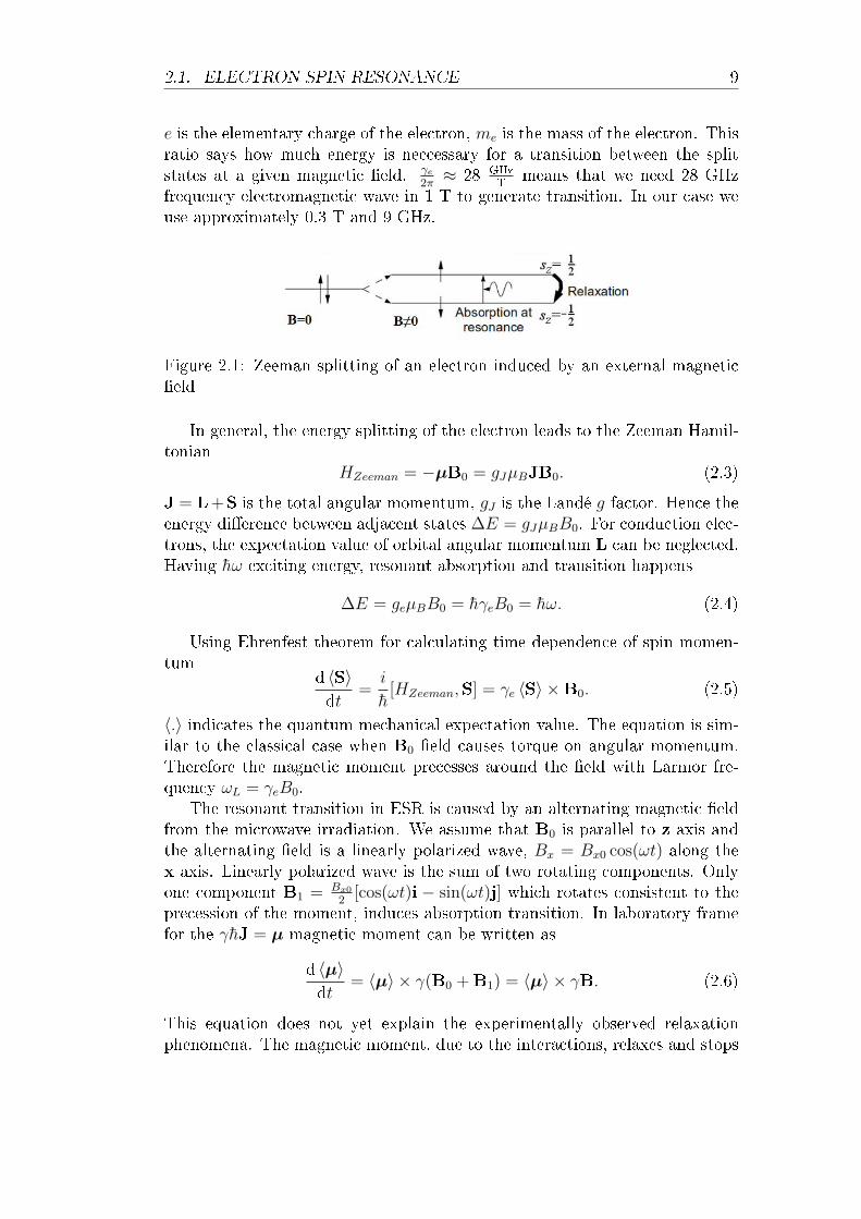
frequency electromagnetic wave in 1 T to generate transition. In our case weuse approximately 0.3 T and 9 GHz.
Figure 2.1: Zeeman splitting of an electron induced by an external magnetic�eld
In general, the energy splitting of the electron leads to the Zeeman Hamil-tonian
HZeeman = −µB0 = gJµBJB0. (2.3)
J = L+S is the total angular momentum, gJ is the Landé g-factor. Hence theenergy di�erence between adjacent states ∆E = gJµBB0. For conduction elec-trons, the expectation value of orbital angular momentum L can be neglected.Having h̄ω exciting energy, resonant absorption and transition happens
∆E = geµBB0 = h̄γeB0 = h̄ω. (2.4)
Using Ehrenfest theorem for calculating time dependence of spin momen-tum
d 〈S〉dt
=i
h̄[HZeeman,S] = γe 〈S〉 ×B0. (2.5)
〈.〉 indicates the quantum mechanical expectation value. The equation is sim-ilar to the classical case when B0 �eld causes torque on angular momentum.Therefore the magnetic moment precesses around the �eld with Larmor fre-quency ωL = γeB0.
The resonant transition in ESR is caused by an alternating magnetic �eldfrom the microwave irradiation. We assume that B0 is parallel to z axis andthe alternating �eld is a linearly polarized wave, Bx = Bx0 cos(ωt) along thex axis. Linearly polarized wave is the sum of two rotating components. Onlyone component B1 = Bx0
2[cos(ωt)i − sin(ωt)j] which rotates consistent to the
precession of the moment, induces absorption transition. In laboratory framefor the γh̄J = µ magnetic moment can be written as
d 〈µ〉dt
= 〈µ〉 × γ(B0 + B1) = 〈µ〉 × γB. (2.6)
This equation does not yet explain the experimentally observed relaxationphenomena. The magnetic moment, due to the interactions, relaxes and stops
2.1. ELECTRON SPIN RESONANCE 10
precessing. It means that after a certain lapse of time, the magnetic momentand the magnetization M = µ
Vsamplestands parallel to the external magnetic
�eld and reaches its equilibrium value. The Bloch equations bring the bestphenomenological description for this problem [2].
dMz(t)
dt= γ[M×B]z +
M0 −Mz(t)
T1
(2.7)
dMx(t)
dt= γ[M×B]x −
Mx(t)
T2
(2.8)
dMy(t)
dt= γ[M×B]y −
My(t)
T2
(2.9)
In general, T1 (spin-lattice or longitudinal) and T2 (spin decoherence ortransversal) relaxation times do not have the same value, but in metals theyare equal T1 = T2 [3]. By solving these equations in a frame of reference whichrotates at an angular frequency ω, we have the x,y magnetization as
M ′x =
χ0ω0
µ0
T2(ω0 − ω)T2
1 + (ω0 − ω)2T 22
B1
M ′y =
χ0ω0
µ0
T21
1 + (ω0 − ω)2T 22
B1.
(2.10)
Herein, the transition angular frequency is: ω0 = γeB0. The rotating frame ofreference is denoted as ' and the equilibrium magnetization reads M0 = χ0B0
µ0where χ0 is the static spin susceptibility, in metals it is the Pauli susceptibilitywhich is temperature dependent.
χ0 = χPauli =1
4µ0(geµB)2ρ(εF )
1
Vc(2.11)
where ρ(εF ) is the density of states at Fermi energy and Vc is the unit cellvolume. In the laboratory frame the magnetization reads:
Mx(t) = M ′x cos(ωt) +M ′
y sin(ωt) (2.12)
The proportional factors are the susceptibilities. Then the form of magnetiza-tion
Mx(t) = (χ′ cos(ωt) + χ′′ sin(ωt))Bx0 = χ(ω)Bx(t) (2.13)
where χ(ω) is dynamical susceptibility and
χ = χ′ − iχ′′. (2.14)
The real part is the dispersive, while the imaginary part is the dissipativeresponse. The absorption is proportional to χ′′ . From the equations abovethe susceptibilities are the following
χ′ =1
2χ0ω0T2
(ω0 − ω)T2
1 + (ω0 − ω)2T 22
(2.15)
2.1. ELECTRON SPIN RESONANCE 11
χ′′ =1
2χ0ω0T2
1
1 + (ω0 − ω)2T 22
. (2.16)
The dynamic susceptibilities are connected by Kramers-Kronig relations [14,13]:
χ′(ω) =1
πP
∫ ∞−∞
dω′χ′′(ω′)1
ω′ − ω(2.17)
χ′′(ω) = − 1
πP
∫ ∞−∞
dω′χ′(ω′)1
ω′ − ω(2.18)
where P denotes the Cauchy principal value. χ′ is the Hilbert transform of−χ′′ [15, 16].
The ESR lineshape is a Lorentzian curve which is proportional to χ′′. Thecalculations above are valid for non-metallic samples. For metallic samplesthe line shape is explained by the theory of Dyson called Conduction ElectronSpin Resonance (CESR) [4].
After discussing the basics of the ESR theory, we discuss some technicalaspects of the ESR signal detection. These are vital for the analysis of theexperiments.
2.1.1 Power detected from ESR
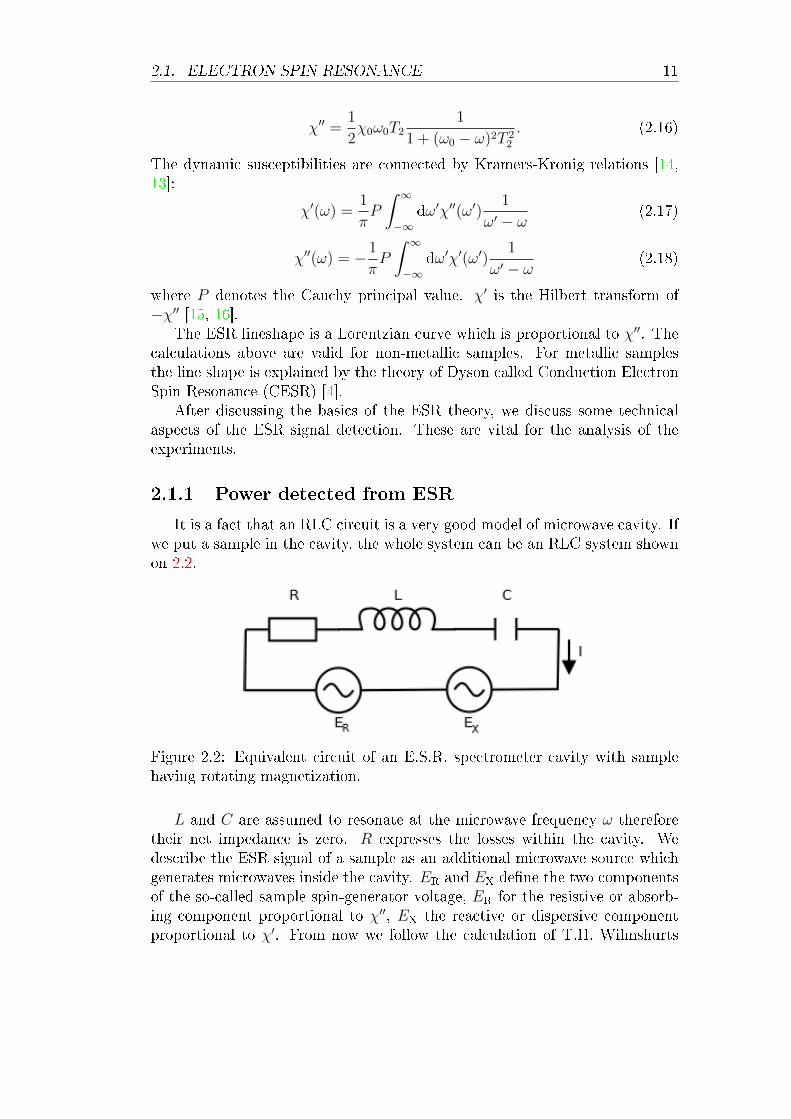
It is a fact that an RLC circuit is a very good model of microwave cavity. Ifwe put a sample in the cavity, the whole system can be an RLC system shownon 2.2.
Figure 2.2: Equivalent circuit of an E.S.R. spectrometer cavity with samplehaving rotating magnetization.
L and C are assumed to resonate at the microwave frequency ω thereforetheir net impedance is zero. R expresses the losses within the cavity. Wedescribe the ESR signal of a sample as an additional microwave source whichgenerates microwaves inside the cavity. ER and EX de�ne the two componentsof the so-called sample spin-generator voltage, ER for the resistive or absorb-ing component proportional to χ′′, EX the reactive or dispersive componentproportional to χ′. From now we follow the calculation of T.H. Wilmshurts
2.1. ELECTRON SPIN RESONANCE 12
[8]. Pa is the available power from the two components
Pa =E2R
8R=E2X
8R. (2.19)
It is neccessary to express ER and EX in terms of Pi which is the power incidenton the cavity. If the cavity is critically coupled this power fully dissipated inthe cavity and no re�ection is observed. Thus Pi = I2R
2. One can show that
ER =2ω
I
∫S
M′B1dV (2.20)
where the volume integral belongs to the sample. The available power fromthe spin generator is:
Pa =(ω∫SM′B1dV )2
2I2R(2.21)
This equation is for the rotating frame of reference. For the laboratory frame
Pa =ω2
16
(∫SMBxdV
Pi
)2
Pi (2.22)
holds. For resonance we obtain: M = χ′′Bx/µ0. The voltage developed by thesample at the detector is proportional1 to
√Pa, so from now we express this
term. √Pa =
ωχ′′∫SB2xdV
4Piµ0
√Pi (2.23)
The term ω∫SB
2xdV
Piis proportional to the product of cavity �lling factor η and
the Q-factor of the cavity. De�nition of Q-factor of the cavity is
Q =ω · Energy storedPower dissipated
. (2.24)
The energy stored in the magnetic �eld of the cavity is given by∫CB
2xdV
2µ0where
the integral goes through the whole cavity. Thus Q = ω∫CB
2xdV
2µ0Piand
√Pa =
χ′′
2·∫SB2xdV∫
CB2xdV
·Q ·√Pi =
χ′′
2· η ·Q ·
√Pi =
χ′′√8η√Q ·
√ω
µ0
∫C
B2xdV
(2.25)where we de�ne η =
∫SB
2xdV∫
CB
2xdV
as cavity �lling factor which indicates how e�-ciently the sample �lls the available magnetic �eld in the cavity. When thesample is saturated by the microwave irradiation the equations above are nolonger appropriate. Let Mmax denote the maximum microwave magnetization
1Commercial ESR spectrometers use mixer to detect microwaves. This method resultsmicrowave voltage, not the power.
2.1. ELECTRON SPIN RESONANCE 13
obtainable without saturation.∫SMdV can be expressed as Mmax
∫ShdV ,
where h has the same spatial variation of M is dimensionless. Equation 2.22then becomes √
Pa =ω
4
(∫S
B2xdV
∫Sh2dV
Pi
) 12
Mmax (2.26)
2.1.2 Mixer and quadrature detection
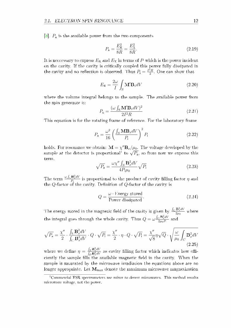
For sensitive detection the modern spectrometers use mixer technique todetect low signal with low noise level. Now we review the basics of mixers.
Figure 2.3: A general mixer
In a mixer three port meet: local oscillator (LO), radio frequency (RF)and intermediate frequency (IF). The term radio frequency generally refersthe high frequency, in our case this is the signal with modulation coming fromthe cavity, so it is the order of 9 GHz. The LO has the same frequency as thesource has. In our measurement the local oscillator is derived from the samesource as the signal before the modulating process. The name of this methodis homodyne detection. Although RF and LO are microwaves, we can handlethem as alternatig voltages.
VLO(t) = ALO cos(ωLOt) (2.27)
LO is neccessary part of the mixers and we can control its power.
VRF(t) = a(t) cos(ωRFt+ φ(t)) (2.28)
Here a(t) and φ(t) are time dependent parts and mean the amplitude andphase modulation. The output IF signal is proportional to the product of RFand LO signal in ideal case.
VIF = KALOa(t) cos(ωLOt) cos(ωRFt+ φ(t)) (2.29)
Where K is a conversion factor which expresses the loss. By trigonometricidentities VIF is written as
VIF =KALO
2a(t) cos[(ωRF−ωLO)t+φ(t)] +
KALO
2a(t) cos[(ωRF +ωLO)t+φ(t)]
(2.30)
2.1. ELECTRON SPIN RESONANCE 14
A tipical mixer contains low-pass �lter therefore the high frequency part isneglectable.
VIF =KALO
2a(t) cos[(ωRF − ωLO)t+ φ(t)] (2.31)
As it is seen the IF signal has lower frequency and lower amplitude than RFbut it contains all parameters for reconstructing the original signal. If wewant IF signal with high amplitude we should enhance ALO. However we mustconsider that the LO port can be saturated and from that point the IF signalwill not be higher. The loss of downconversion is de�ned as
PIFPRF
=
(KALO
2
)2
. (2.32)
KALO has tipical value about 1. Loss in dB unit is about 10 log10(14) = −6dB.
This value varies from −3dB ot −10dB. The quantity which indicates the lossof the mixer is conversion loss (CL):
CL = −10 log10
(PIFPRF
)(2.33)
and its value varies from 3 dB to 10 dB. Obviously low CL is desirable. Theformulas show that we must keep the LO power near the saturation powerbecause if we work with less LO power the CL is increased [9].
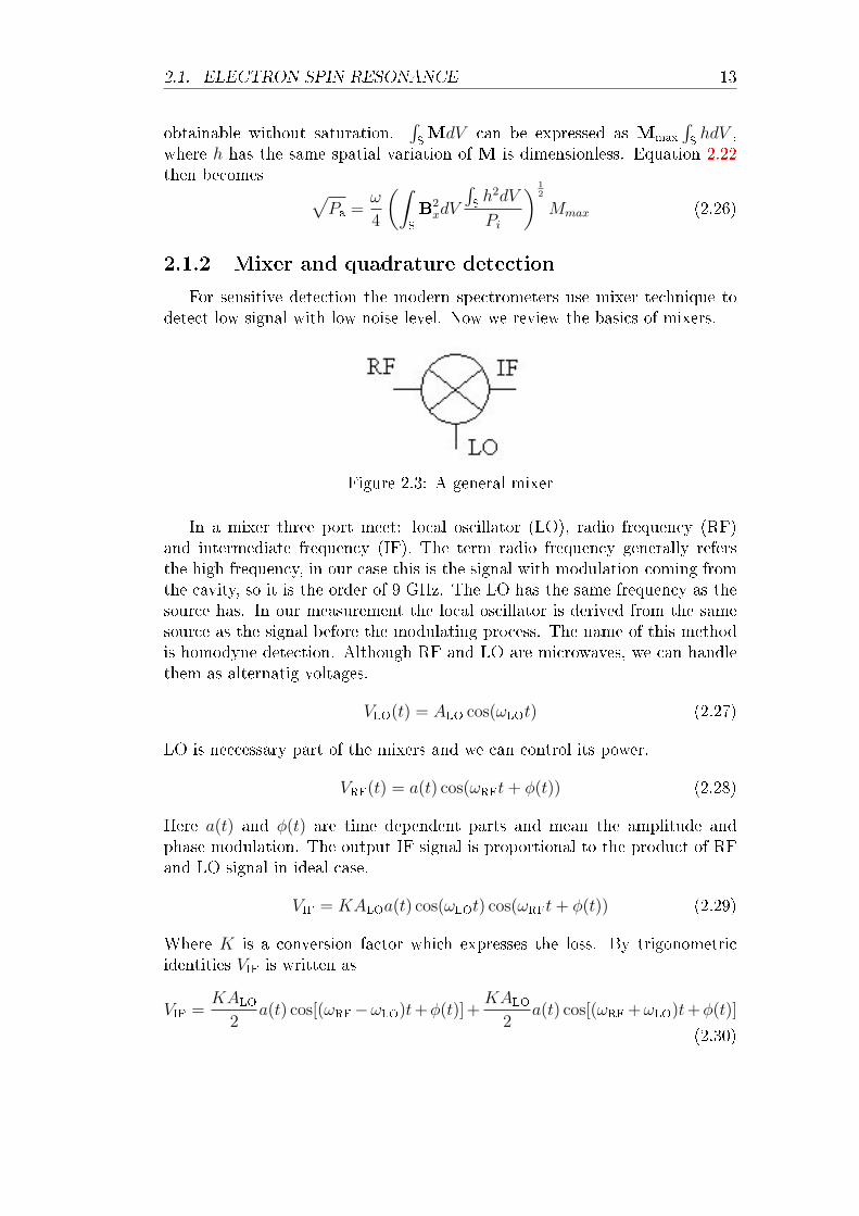
In our measurement we use an IQ mixer (Marki IQ 0618) with which thequadrature detection is possible. The IQ mixer splits RF and LO in two equal
Figure 2.4: Schematics of an IQ mixer [10]
part gives 90◦ shift for one of splitted LO. It has two output; "Q" indicates thequadrature signal that is product of shifted LO and RF, "I" output indicatesthe in-phase signal that is product if in-phase LO and RF. The resultant twocomponents are perpendicular. Only with this type of detection we are able tomeasure Kramers-Kronig pairs of susceptibility simultaneously. In the masterthesis we employ IQ mixer to justify the validity of the linear response theory.IQ mixer detection is also required when the LO and RF have di�erent fre-quencies and the sign of the IF needs to be known, too. E.g. this is employedin pulsed ESR and NMR spectroscopies.
2.1. ELECTRON SPIN RESONANCE 15
2.1.3 Relationship between the complex dynamic spin-
susceptibility and microwave phase
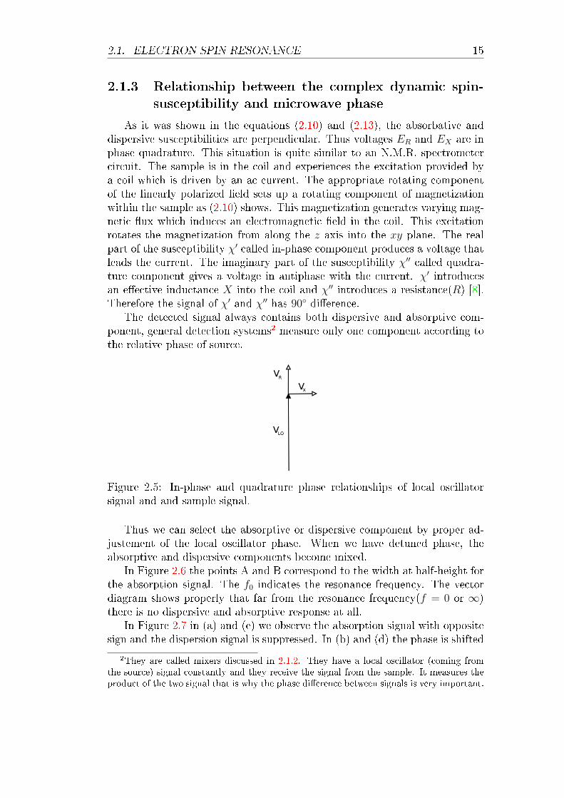
As it was shown in the equations (2.10) and (2.13), the absorbative anddispersive susceptibilities are perpendicular. Thus voltages ER and EX are inphase quadrature. This situation is quite similar to an N.M.R. spectrometercircuit. The sample is in the coil and experiences the excitation provided bya coil which is driven by an ac current. The appropriate rotating componentof the linearly polarized �eld sets up a rotating component of magnetizationwithin the sample as (2.10) shows. This magnetization generates varying mag-netic �ux which induces an electromagnetic �eld in the coil. This excitationrotates the magnetization from along the z axis into the xy plane. The realpart of the susceptibility χ′ called in-phase component produces a voltage thatleads the current. The imaginary part of the susceptibility χ′′ called quadra-ture component gives a voltage in antiphase with the current. χ′ introducesan e�ective inductance X into the coil and χ′′ introduces a resistance(R) [8].Therefore the signal of χ′ and χ′′ has 90◦ di�erence.
The detected signal always contains both dispersive and absorptive com-ponent, general detection systems2 measure only one component according tothe relative phase of source.
Figure 2.5: In-phase and quadrature phase relationships of local oscillatorsignal and and sample signal.
Thus we can select the absorptive or dispersive component by proper ad-justement of the local oscillator phase. When we have detuned phase, theabsorptive and dispersive components become mixed.
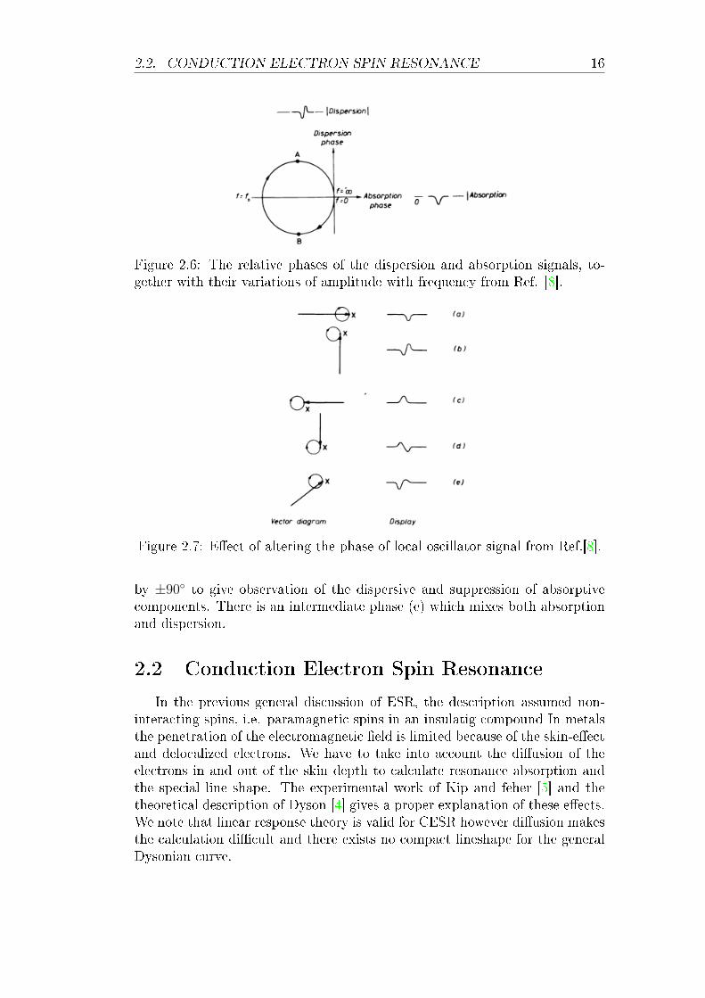
In Figure 2.6 the points A and B correspond to the width at half-height forthe absorption signal. The f0 indicates the resonance frequency. The vectordiagram shows properly that far from the resonance frequency(f = 0 or ∞)there is no dispersive and absorptive response at all.
In Figure 2.7 in (a) and (e) we observe the absorption signal with oppositesign and the dispersion signal is suppressed. In (b) and (d) the phase is shifted
2They are called mixers discussed in 2.1.2. They have a local oscillator (coming fromthe source) signal constantly and they receive the signal from the sample. It measures theproduct of the two signal that is why the phase di�erence between signals is very important.
2.2. CONDUCTION ELECTRON SPIN RESONANCE 16
Figure 2.6: The relative phases of the dispersion and absorption signals, to-gether with their variations of amplitude with frequency from Ref. [8].
Figure 2.7: E�ect of altering the phase of local oscillator signal from Ref.[8].
by ±90◦ to give observation of the dispersive and suppression of absorptivecomponents. There is an intermediate phase (e) which mixes both absorptionand dispersion.
2.2 Conduction Electron Spin Resonance
In the previous general discussion of ESR, the description assumed non-interacting spins, i.e. paramagnetic spins in an insulatig compound In metalsthe penetration of the electromagnetic �eld is limited because of the skin-e�ectand delocalized electrons. We have to take into account the di�usion of theelectrons in and out of the skin depth to calculate resonance absorption andthe special line shape. The experimental work of Kip and feher [5] and thetheoretical description of Dyson [4] gives a proper explanation of these e�ects.We note that linear response theory is valid for CESR however di�usion makesthe calculation di�cult and there exists no compact lineshape for the generalDysonian curve.
2.2. CONDUCTION ELECTRON SPIN RESONANCE 17
From the Maxwell's equations we get a modi�ed expression for the conduc-tive medium:
∆B = µε∂2B
∂t2+ µσ
∂B
∂t. (2.34)
The solution of this equation can be a plane wave:
B(x, t) = B0ei(kx−ωt) (2.35)
where B0 is the amplitude of the ac magnetic �eld at the sample surface. Aftersubstituting, a complex wave number is given by
k =√µεω2 + iµσω = i
1
δSkin + κ(2.36)
where κ = ω[(
εµ2
) (√1 + ( σ
ωε)2 − 1
)] 12 . The general expression for the skin
depth is δSkin = 1ω
[(εµ2
) (√1 + ( σ
ωε)2 + 1
)]− 12 but for metals this expression
can be simpli�ed
δSkin =
√2
µσω(2.37)
where µ and ε are the total permeability and permittivity respectively and σis the conductivity. If the electromagnetic waves propagates along the x axis,then the ac magnetic �eld strength is given by
B ∼ e− xδSkin · e·i(κx−ωt) (2.38)
in the sample. We emphasize that going through the x axis into the samplethe phase of exciting electromagnetic �eld continuously changes, thus everyplane perpendicular to the x axis gets di�erent excitation. This fact resultsin a di�erent line shape as compared to a non-metallic sample. According toDyson, Kip and Feher we distinguish two main cases: region of normal andanomalous skin e�ect. This distinction is based on whether the mean free-pathδ
�lis smaller (normal) or larger (anomalous) than the skin-depth. The latter
occurs for very high frequency electromagnetic radiation (in the THz range)for very pure metals. The normal skin e�ect regime occurs in Li at roomtemperature and 9 GHz excitation so we focus on this regime only.
The general problems is to calculate the magnetization produced by a givenB1, and to �nd a self-consistent solutions of Maxwell's equations to expressthe relationships between B1 and M. The magnetization is carried around bythe electrons as they di�use in the metal. This fact makes the problem quiteunusual and more involved. The assumptions of Dyson were the following:
1. All electrons which carry the magnetization lie at the top of the Fermidistribution of conduction electrons and move with constant Fermi ve-locity, vF .
2.2. CONDUCTION ELECTRON SPIN RESONANCE 18
2. An electron changes its direction (momentum) as a result of collisionwith other electrons, lattice vibrations, etc. Then each electron loses itsmemory of its direction of motion, so it moves as an independent classicalparticle randomly.
3. The spin of each electron is only very weakly coupled to the electron'sorbital motion and it is una�ected by collision. However the weak spin-orbit coupling is taken into account in the relaxation time T1. There isa probability e−
tT1 that the spin state will be undisturbed by collision
during a time interval t.
Let F (r, r) denote the probability distribution for the position r of oneelectron at time t. If the time scale is much larger then mean collision timeτ =
δ�l
vF, classical di�usion equation is valid
∂F
∂t=
1
3vF δ�l
∆F, (2.39)
and the boundary condition is n · gradF = 0 where n is the normal vector atany point of the metal surface. The ESR line shape is normally described as afunction of parameters like spin susceptibility χ, spin relaxation time T1, andg-factor. However in metals we need two extra parameters to get describe theline shape. The �rst is de�ned as R =
√TDT2
where TD =3δ2Skin2vF δ�l
is the electrondi�usion time across the skin depth. The second is TT, the time it takes for theelectron to di�use through the whole sample. ESR spectroscopy measures theabsorbed power in the sample by the so-called cavity perturbation technique.Therefore it is crucial to determine the power-frequency P (ω) function. Nowwe distinguish two di�erent cases. The simpler one is when TT << TD, a thick-ness of the sample/�lm is smaller than the skin depth. The power absorbedis
Pa =ωB2
1V ω0χ0T2
µ04(1 + (ω − ω0)2T 22 )
(2.40)
where V = volume of the sample, B1 =amplitude of linearly polarized alter-nating magnetic �eld. This result totally independent of di�usion and givesLorentz line with the half width 1
T2. The other case when TT >> TD and
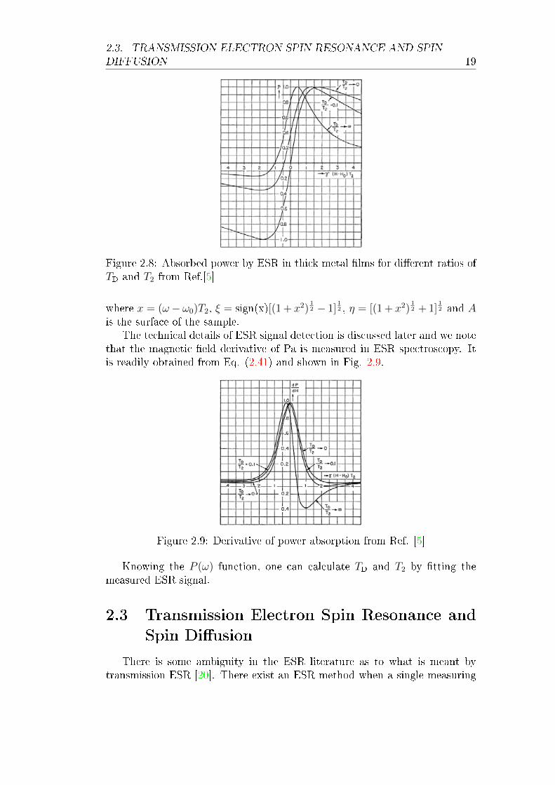
TT >> T2 is important for us. Taking into account the assumptions of Dysonthe absorbed power (Fig. 2.8) is:
Pa = −1
8(δSkinωB
21Aω0χ0T2)R2
{R4(x2 − 1) + 1− 2R2x
µ0[(R2x− 1)2 +R4]2·
(2ξ
R(1 + x2)12
+R2(x+ 1)− 3
)+
2R2 − 2xR4
((R2x− 1)2 +R4)2·
(2η
R(1 + x2)12
+R2(x− 1)− 3
)}(2.41)
2.3. TRANSMISSION ELECTRON SPIN RESONANCE AND SPIN
DIFFUSION 19
Figure 2.8: Absorbed power by ESR in thick metal �lms for di�erent ratios ofTD and T2 from Ref.[5]
where x = (ω− ω0)T2, ξ = sign(x)[(1 + x2)12 − 1]
12 , η = [(1 + x2)
12 + 1]
12 and A
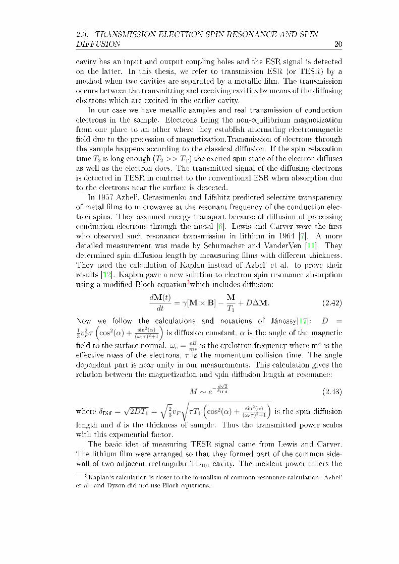
is the surface of the sample.The technical details of ESR signal detection is discussed later and we note
that the magnetic �eld derivative of Pa is measured in ESR spectroscopy. Itis readily obtained from Eq. (2.41) and shown in Fig. 2.9.
Figure 2.9: Derivative of power absorption from Ref. [5]
Knowing the P (ω) function, one can calculate TD and T2 by �tting themeasured ESR signal.
2.3 Transmission Electron Spin Resonance andSpin Di�usion
There is some ambiguity in the ESR literature as to what is meant bytransmission ESR [20]. There exist an ESR method when a single measuring
2.3. TRANSMISSION ELECTRON SPIN RESONANCE AND SPIN
DIFFUSION 20
cavity has an input and output coupling holes and the ESR signal is detectedon the latter. In this thesis, we refer to transmission ESR (or TESR) by amethod when two cavities are separated by a metallic �lm. The transmissionoccurs between the transmitting and receiving cavities bz means of the di�usingelectrons which are excited in the earlier cavity.
In our case we have metallic samples and real transmission of conductionelectrons in the sample. Electrons bring the non-equilibrium magnetizationfrom one place to an other where they establish alternating electromagnetic�eld due to the precession of magnetization.Transmission of electrons throughthe sample happens according to the classical di�usion. If the spin relaxationtime T2 is long enough (T2 >> TT) the excited spin state of the electron di�usesas well as the electron does. The transmitted signal of the di�using electronsis detected in TESR in contrast to the conventional ESR when absorption dueto the electrons near the surface is detected.
In 1957 Azbel', Gerasimenko and Lifshitz predicted selective transparencyof metal �lms to microwaves at the resonant frequency of the conduction elec-tron spins. They assumed energy transport because of di�usion of precessingconduction electrons through the metal [6]. Lewis and Carver were the �rstwho observed such resonance transmission in lithium in 1964 [7]. A moredetailed measurement was made by Schumacher and VanderVen [11]. Theydetermined spin di�usion length by meausuring �lms with di�erent thickness.They used the calculation of Kaplan instead of Azbel' et al. to prove theirresults [12]. Kaplan gave a new solution to electron spin resonance absorptionusing a modi�ed Bloch equation3which includes di�usion:
dM(t)
dt= γ[M×B]− M
T1
+D∆M. (2.42)
Now we follow the calculations and notations of Jánossy[17]: D =13v2F τ(
cos2(α) + sin2(α)(ωcτ)2+1
)is di�usion constant, α is the angle of the magnetic
�eld to the surface normal. ωc = eBm∗ is the cyclotron frequency where m* is the
e�ective mass of the electrons, τ is the momentum collision time. The angledependent part is near unity in our measurements. This calculation gives therelation between the magnetization and spin di�usion length at resonance:
M ∼ e− d
√2
δDi� (2.43)
where δDi� =√
2DT1 =√
23vF
√τT1
(cos2(α) + sin2(α)
(ωcτ)2+1
)is the spin di�usion
length and d is the thickness of sample. Thus the transmitted power scaleswith this exponential factor.
The basic idea of measuring TESR signal came from Lewis and Carver.The lithium �lm were arranged so that they formed part of the common side-wall of two adjacent rectangular TE101 cavity. The incident power enters the
3Kaplan's calculation is closer to the formalism of common resonance calculation. Azbel'et al. and Dyson did not use Bloch equations.
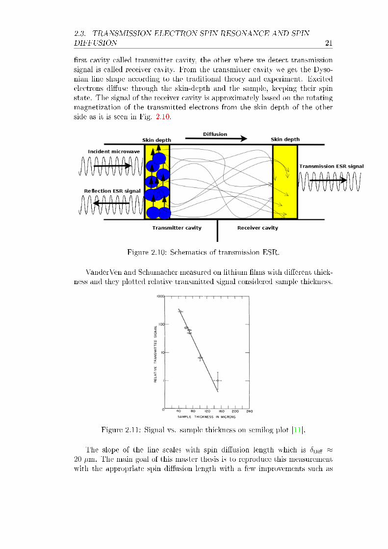
2.3. TRANSMISSION ELECTRON SPIN RESONANCE AND SPIN
DIFFUSION 21
�rst cavity called transmitter cavity, the other where we detect transmissionsignal is called receiver cavity. From the transmitter cavity we get the Dyso-nian line shape according to the traditional theory and experiment. Excitedelectrons di�use through the skin-depth and the sample, keeping their spinstate. The signal of the receiver cavity is approximately based on the rotatingmagnetization of the transmitted electrons from the skin depth of the otherside as it is seen in Fig. 2.10.
Figure 2.10: Schematics of transmission ESR.
VanderVen and Schumacher measured on lithium �lms with di�erent thick-ness and they plotted relative transmitted signal considered sample thickness.
Figure 2.11: Signal vs. sample thickness on semilog plot [11].
The slope of the line scales with spin di�usion length which is δDi� ≈20 µm. The main goal of this master thesis is to reproduce this measurementwith the appropriate spin di�usion length with a few improvements such as
2.3. TRANSMISSION ELECTRON SPIN RESONANCE AND SPIN
DIFFUSION 22
modulated ESR, low noise quadrature detection. The latter is possible dueto the availability of low noise preampli�er (which were not available in the1960's) and compact IQ mixer detectors.

Chapter 3
Results and discussions
In this chapter we discuss the steps which led us to TESR measure-ments. We give detailed discussion of quadrature ESR detection, cavity sys-tem, impedance matching and �nally we calculate spin di�usion length oflithium from the measured spectra. Our intention was to reproduce an ear-lier TESR experiment on lithium with a modern instrumentation: the use oflow noise microwave preampli�ers, IQ mixer detectors. In addition we employmagnetic �eld modulation which was not performed in the original experimentsin Refs. [7, 11].
3.1 Conventional ESR with quadrature detec-tion
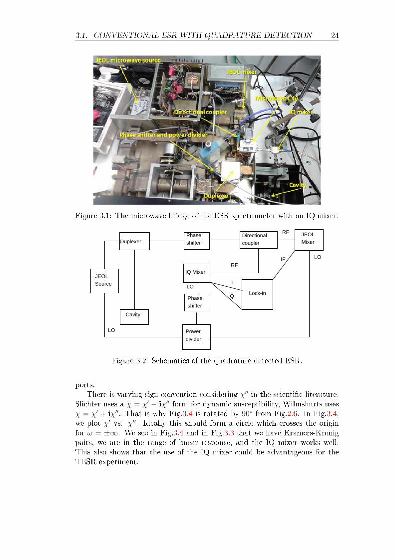
We built a hybrid ESR microwave circuit by using of the commercial JEOLspectrometer and IQ mixer and Low Noise Ampli�er. A photograph of thesystem is shown in Fig.3.1.
The JEOL spectrometer has a built-in AFC system which is employedherein. The 200 mW signal of the JEOL source is divided to provide theLO for the built-in mixer of the JEOL spectrometer and for the present IQmixer, too. The ESR signal (RF) is also divided between the two mixers. Thiscon�guration allows to detect the IQ signal while the spectrometer's AFC isworking properly. A block diagram is shown in Fig. 3.2.
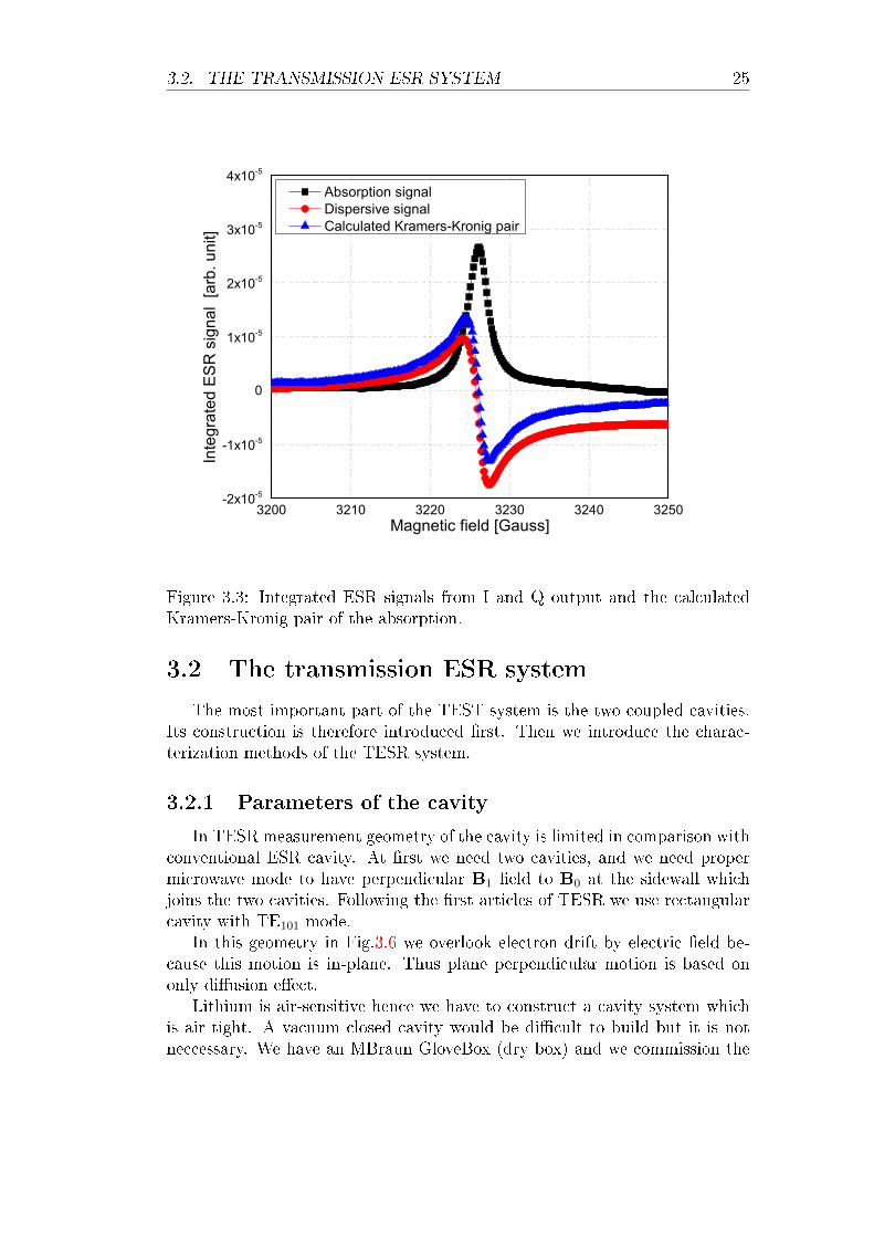
We performed measurement on an ESR standard: DPPH.In the measurement we get derivative of absorptional signal (proportinal
to χ′′) and derivative of dispersive signal (proportinal to χ′). To check thevalidity of the use of the IQ detection, we perform a numerical Kramers-Kronigtraonsformation (which is called discrete Hilbert transform) of the absorptionsignal to obtain the numerical dispersion signal. The lines do not go exactlyto zero and there is a little di�erence between the measured and calculateddispersion line. The reason is some o�set problem and imperfection of mixerLO port. Probably there is not an exact 90◦ di�erence between the I and Q
23
3.1. CONVENTIONAL ESR WITH QUADRATURE DETECTION 24
Figure 3.1: The microwave bridge of the ESR spectrometer with an IQ mixer.
JEOL Source
Directionalcoupler
Powerdivider
Cavity
Phaseshifter
IQ Mixer
Duplexer
Phaseshifter
LO
LO
RF
JEOL Mixer
RF
LO
Lock-in
I
Q
IF
Figure 3.2: Schematics of the quadrature detected ESR.
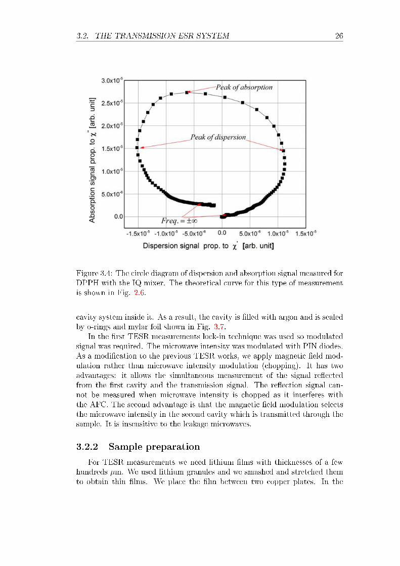
ports.There is varying sign convention considering χ′′ in the scienti�c literature.
Slichter uses a χ = χ′ − iχ′′ form for dynamic susceptibility, Wilmshurts usesχ = χ′ + iχ′′. That is why Fig.3.4 is rotated by 90◦ from Fig.2.6. In Fig.3.4,we plot χ′ vs. χ′′. Ideally this should form a circle which crosses the originfor ω = ±∞. We see in Fig.3.4 and in Fig.3.3 that we have Kramers-Kronigpairs, we are in the range of linear response, and the IQ mixer works well.This also shows that the use of the IQ mixer could be advantageous for theTESR experiment.
3.2. THE TRANSMISSION ESR SYSTEM 25
3200 3210 3220 3230 3240 3250-2x10⁻⁵
-1x10⁻⁵
0
1x10⁻⁵
2x10⁻⁵
3x10⁻⁵
4x10⁻⁵
Inte
grat
ed E
SR
sig
nal
[arb
. uni
t]
Magnetic field [Gauss]
Absorption signal Dispersive signal Calculated Kramers-Kronig pair
Figure 3.3: Integrated ESR signals from I and Q output and the calculatedKramers-Kronig pair of the absorption.
3.2 The transmission ESR system
The most important part of the TEST system is the two coupled cavities.Its construction is therefore introduced �rst. Then we introduce the charac-terization methods of the TESR system.
3.2.1 Parameters of the cavity
In TESR measurement geometry of the cavity is limited in comparison withconventional ESR cavity. At �rst we need two cavities, and we need propermicrowave mode to have perpendicular B1 �eld to B0 at the sidewall whichjoins the two cavities. Following the �rst articles of TESR we use rectangularcavity with TE101 mode.
In this geometry in Fig.3.6 we overlook electron drift by electric �eld be-cause this motion is in-plane. Thus plane perpendicular motion is based ononly di�usion e�ect.
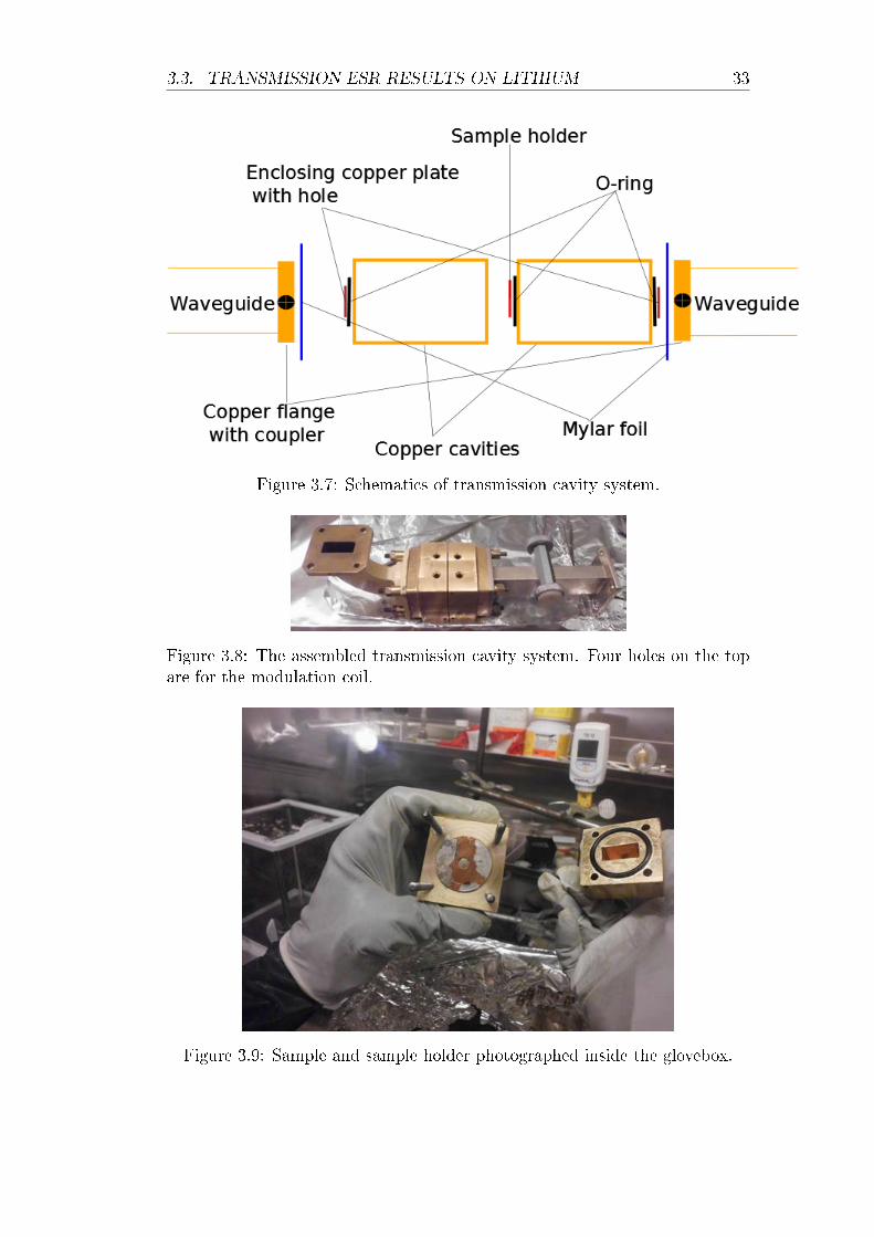
Lithium is air-sensitive hence we have to construct a cavity system whichis air tight. A vacuum closed cavity would be di�cult to build but it is notneccessary. We have an MBraun GloveBox (dry box) and we commission the
3.2. THE TRANSMISSION ESR SYSTEM 26
Figure 3.4: The circle diagram of dispersion and absorption signal measured forDPPH with the IQ mixer. The theoretical curve for this type of measurementis shown in Fig. 2.6.
cavity system inside it. As a result, the cavity is �lled with argon and is sealedby o-rings and mylar foil shown in Fig. 3.7.
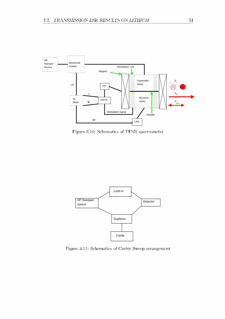
In the �rst TESR measurements lock-in technique was used so modulatedsignal was required. The microwave intensity was modulated with PIN diodes.As a modi�cation to the previous TESR works, we apply magnetic �eld mod-ulation rather than microwave intensity modulation (chopping). It has twoadvantages: it allows the simultaneous measurement of the signal re�ectedfrom the �rst cavity and the transmission signal. The re�ection signal can-not be measured when microwave intensity is chopped as it interferes withthe AFC. The second advantage is that the magnetic �eld modulation selectsthe microwave intensity in the second cavity which is transmitted through thesample. It is insensitive to the leakage microwaves.
3.2.2 Sample preparation
For TESR measurements we need lithium �lms with thicknesses of a fewhundreds µm. We used lithium granules and we smashed and stretched themto obtain thin �lms. We place the �lm between two copper plates. In the
3.2. THE TRANSMISSION ESR SYSTEM 27
middle of the copper plate there is a hole where the sample is placed. We putsome lithium �lm on the surface of the copper plate which is in contact withthe surface of the cavity in order to get good plumbing and to avoid microwaveleakage.
There are two requirements for the construction of the transmission cavitysystem. Namely, the air tight composition and the reduction of microwaveleakage between the cavities. The �rst requirement is ful�lled with the use ofo-rings and vacuum grease. However it does not matter how strong we jointwo cavities, we experience some leakage power in the second cavity1 fromthe �rst one. Having the sample between the cavities, the leakage is about50-60 dB. It gives us a a lower limit for the magnitude of the TESR signal.Namely, the sample inside the �rst cavity radiates an ESR signal (which isalso magnetic �eld modulated) which is not related to the TESR signal butenters the second cavity in any case together with the leakage. This means noTESR signal can be observed which is smaller than 60 dB of the ESR signalinside the �rst cavity. Transmission signal scales with the factor of e−
dδDi� . In
practice if the sample has more than 250-300 µm thickness we observe only theleakage signal in the receiver cavity. We performed several experiments thatthis leakage comes from only the joint of two cavity and not from the joint ofthe �anges or waveguides. Another limitation occurs together with the leakage:an unmodulated (or DC) microwave signal enters the second cavity which doesnot a�ect the lock-in measurement, however it can saturated the LNA beforethe mixer or the RF port of the mixer itself. To hand this power, we alwayschecked that the LNA works outside saturation and also that the mixer is notsaturated either.
3.2.3 Characterization of the TESR system
In order to characterize our system we made several control experiments.The very �rst experiment was on DPPH. We put the sample inside the cavitysystem but we place an o-ring and separation copper plate with hole betweentwo cavity. Diameter of hole is the same as the coupling plane. We detectboth signals; from the transmitter cavity in re�ection and from the receivercavity in transmission. We found that both ESR signal is in the same orderof magnitude if both cavities are critically coupled. It means that our cavitydesign is symmetric.
Other measurement was about leakage. We had to make the followingmeasurements before every TESR experiment in order to determine resonancefrequency of the cavity, Q factor, and leakage power. Now we discuss an idealcase when there is no sample but only a copper plate with no holes between thecavities. We determine resonant frequencies and Q factor with the so-calledCavity Sweep method. Then we measure leakage power with a modi�ed Cavity
1This problem is symmetric that is why no use to di�erentiate transmitter and receivercavity.
3.3. TRANSMISSION ESR RESULTS ON LITHIUM 28
Sweep method as shown in Fig.3.11.We sweep the frequency and we measure the re�ected power from the trans-
mitter cavity. When we �nd the resonant frequency of the cavity we measurezero re�ected power as it is critically coupled. We record the re�ected curveand we �t a Lorentz curve shown in Fig.3.12.
The curve of receiver cavity is quite similar except the resonance frequencywhich can be somewhat di�erent (up to 40 MHz) and the Q factor can bedi�erent, too.Although the two cavities were manufactured to have the samelength and cross section, their parameters are not the same. To join everypart of the cavity system properly is technically di�cult which results in thedi�erence of the parameters. This problem is present in every con�guration oftransmission cavity system.The leakage is determined in a di�erent con�guration as shown in Fig.3.13.
We sweep the frequency and we detect transmitted signal from the receivercavity. This signal power is much lower than the re�ected signal that is whywe have to amplify it.
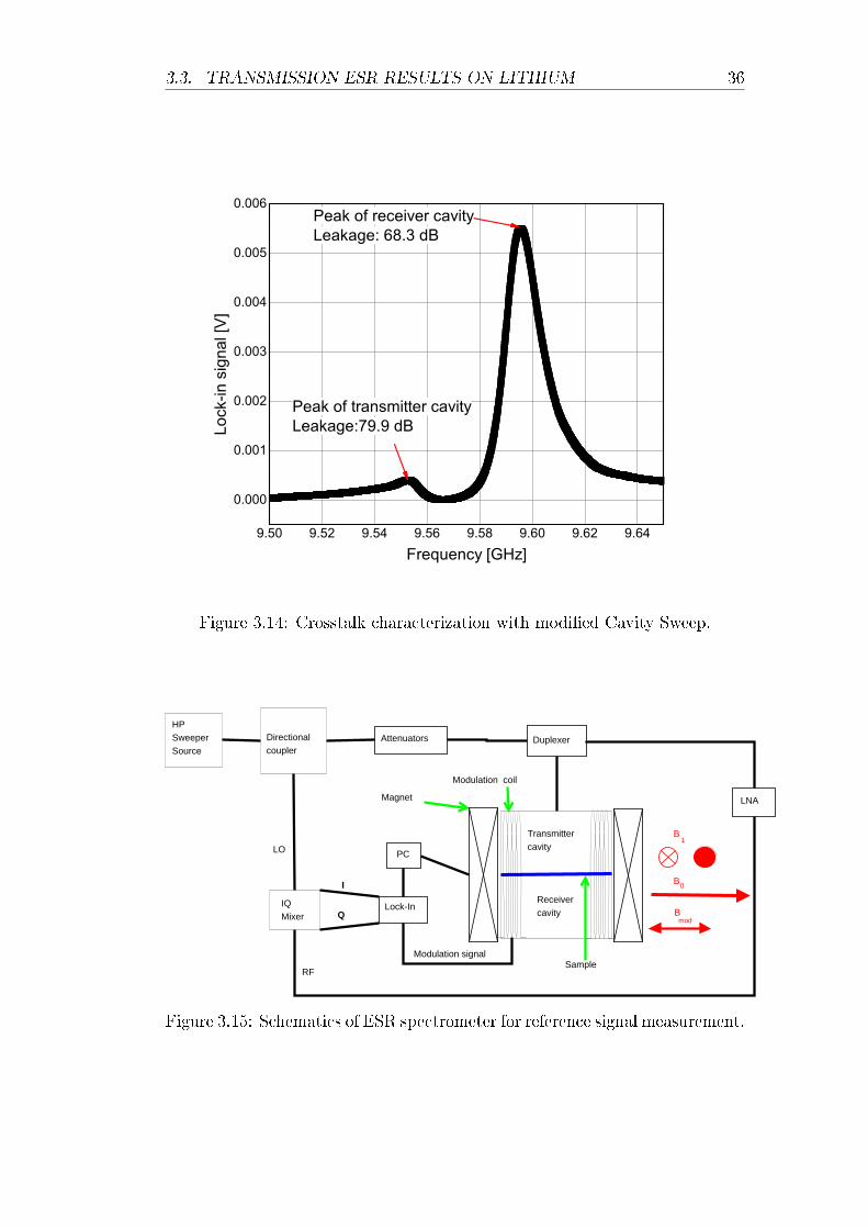
In Fig.3.14 the peaks correspond the resonance frequency of the corre-sponding cavity. Leakage is calculated from voltage-power characterization ofthe detector. 79.9 dB was the smallest leakage we detected. Normally, withlithium sample the leakage is about 60 dB. If the expected transmission signalis the order of the leakage we cannot measure it. As a result of the substantialleakage, we follow a di�erent route from the previous approaches, where muchlower (up to 180 dB) leakage were attained. We measure the magnitude of theTESR signal and compare it to the ESR signal which is re�ected back fromthe transmitting cavity. This way the TESR signal is accurately calibrated.The arrangement of re�ection ESR measurement shown in Fig.3.15.
3.3 Transmission ESR results on lithium
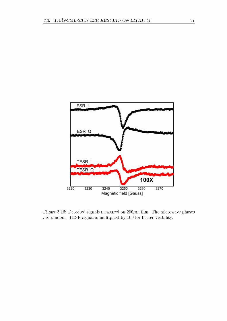
We prepared four lithium samples with di�erent thickness. Sample with90 µm and 150 µm thickness were prepared as we mentioned in the previoussection. Because of technical reasons, the thicker samples were wider andlonger thus they covered the whole cross section of cavity and we did notuse sample holder. We measured the re�ection and transmission ESR signalswith the IQ mixer for every sample. The ESR intensity contains the adequateinformation so there is no speci�c microwave phase adjustment. We obtainedthe curves like in Fig. 3.16 for every thickness.
The incident power were 20 dBm but in re�ection ESR measurements wehad to attenuate the power because of the because of the not optimal isolationof the duplexer (a microwave circulator). We calculated the resulting intensity(T,R) of TESR and re�ection ESR from the peak-to-peak I and Q voltages.
T\R =√I2T\R + Q2
T\R (3.1)
3.3. TRANSMISSION ESR RESULTS ON LITHIUM 29
Thus the intensity is proportional to the microwave voltages. We measured thecavity resonance and leakage before every TESR experiment. In the leakagemeasurements we found that there are two resonant frequency2 with di�erentleakage. We measured on that frequency which had smaller leakage. In thiscase the impedance were not matched perfectly between the two cavities. InAppendix A we show that it is not so disturbing e�ect.
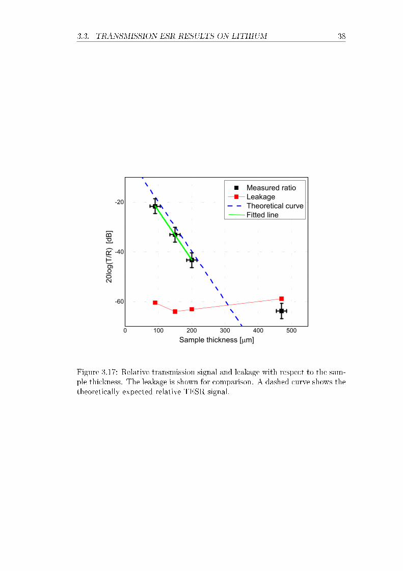
As it is shown in Fig.3.17 where the leakage is higher than the expectedsignal at 480 µm, we are not able to measure TESR. We �tted a line accordingto the following equation:
20 log
(T
R
)= 20 log
(Ce− d
2δD
)(3.2)
δD = vF
√13τT1 is the e�ective spin di�usion length. The intensities are propor-
tional to the microwave voltage thus factor of two in the exponent comes fromthe general relation between power and voltage
√P ∼ U . C is an empirical
constant. We chose C = 1 in the theoretical curve. In this curve T1 = 10−7 s,vF = 1.3·106m
s, τ = 8.462·10−15 s and they give δD = 21.8 µm according to the
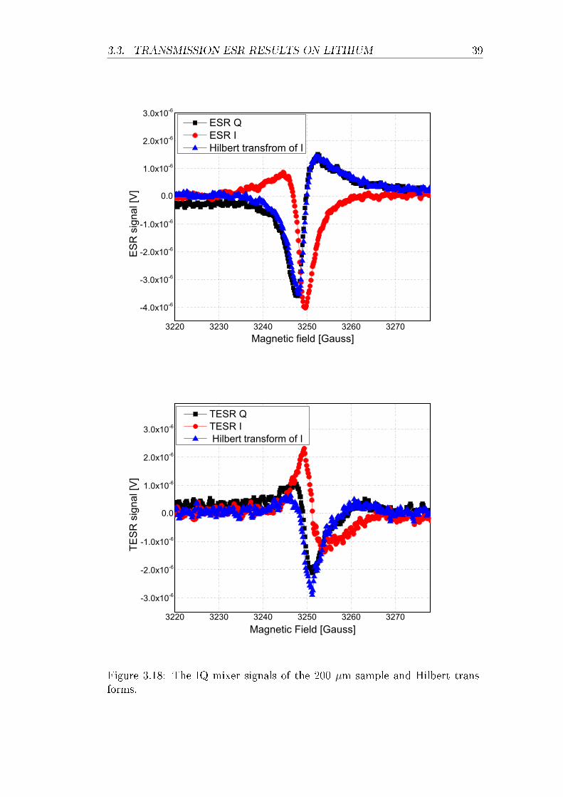
calculation of Schumacher and VanderVen [11]. They measured δD = 22.6 µm.Our �tted line gives δD = 22.1 µm. Although the measured result is quite closeto the publicated one, there is a huge uncertanity considering τ and T1. We donot know the concentration of impurities of our lithium �lms. The agreementbetween the experimental result and the theoretical curve con�rms that wedid observe the TESR signal in lithium.
3.3.1 The validity of the Kramers-Kronig pairs in
quadrature detected TESR
We measured the I and Q signals of TESR and ESR measurements with anarbitrary phase. The signals are proportional to the derivative of dynamic spinsusceptibility with respect to ω. The arbitrary phase φ causes the mixture ofabsorption and dispersive susceptibilites in I and Q. I and Q signals are stillperpendicular.
I ∼ cos(φ)dχ′(ω)
dω+ sin(φ)
dχ′′(ω)
dω(3.3)
Q ∼ − sin(φ)dχ′(ω)
dω+ cos(φ)
dχ′′(ω)
dω(3.4)
Considering some basic properties of the Hilbert transform we prove thatQ signal is the Hilbert transform of I signal, consequently we measured aKramers-Kronig pair and ESR and TESR both satisfy the linear responsetheory.
2 The tunable cavity was not ready by that time.
3.3. TRANSMISSION ESR RESULTS ON LITHIUM 30
H indicates the Hilbert transform, g(t) is a signal, H[g(t)] is the transformedsignal, t is a general variable.
H[g(t)] =1
π
∫ ∞−∞
g(τ)
t− τdτ =
1
π
∫ ∞−∞
g(t− τ)
τ(3.5)
H[g(t)] is the convolution of 1πtwith the signal g(t) [18]. The Hilbert transform
is linear from the fact, that the Hilbert transform is the output of a linearsystem, then
H[ag(t) + bh(t)] = aH[g(t)] + bH[h(t)] (3.6)
where a and b are arbitrary complex numbers. Other important property isthat Hilbert transform of the derivative of a signal is the derivative of theHilbert transform.
H[dg(t)
dt
]=
ddtH[g(t)] (3.7)
According to Leibniz's Integral Rule
ddc
∫ b
a
f(x, c)dx =
∫ b
a
∂f(x, c)
∂cdx (3.8)
if a and b are not the function of c. In our case a and b are de�nite. Now
(3.9)
ddtH[g(t)] =
ddt
1
π
∫ ∞−∞
g(t− τ)
τdτ
=1
π
∫ ∞−∞
g′(t− τ)
τdτ
= H[g′(t)]
where g′(t) = dg(t)dt
.There is a slight di�erence among (2.17),(2.18) and Hilbert transform. The
integration goes with the �rst term of denominator in formulas of Kramers-Kronig but in Hilbert transform it goes with the second term. The result reads:H[χ′′] = −H[χ′] and H[χ′] = H[χ′′]. The Hilbert transform of I is:
(3.10)
H[I] ∼ Hddt
(cos(φ)χ′ + sin(φ)χ′′)
∼ ddt
(cos(φ)H[χ′] + sin(φ)H[χ′′])
∼ ddt
(− sin(φ)χ′ + cos(φ)χ′′)
∼ Q
where χ′ and χ′′ are ω dependent functions.The OriginLab program calculated the discrete Hilbert transforms of the
signals. In Fig. 3.18 we show that the IQ mixer works properly and linearresponse theory is still valid.
3.3. TRANSMISSION ESR RESULTS ON LITHIUM 31
3.3.2 Control experiment
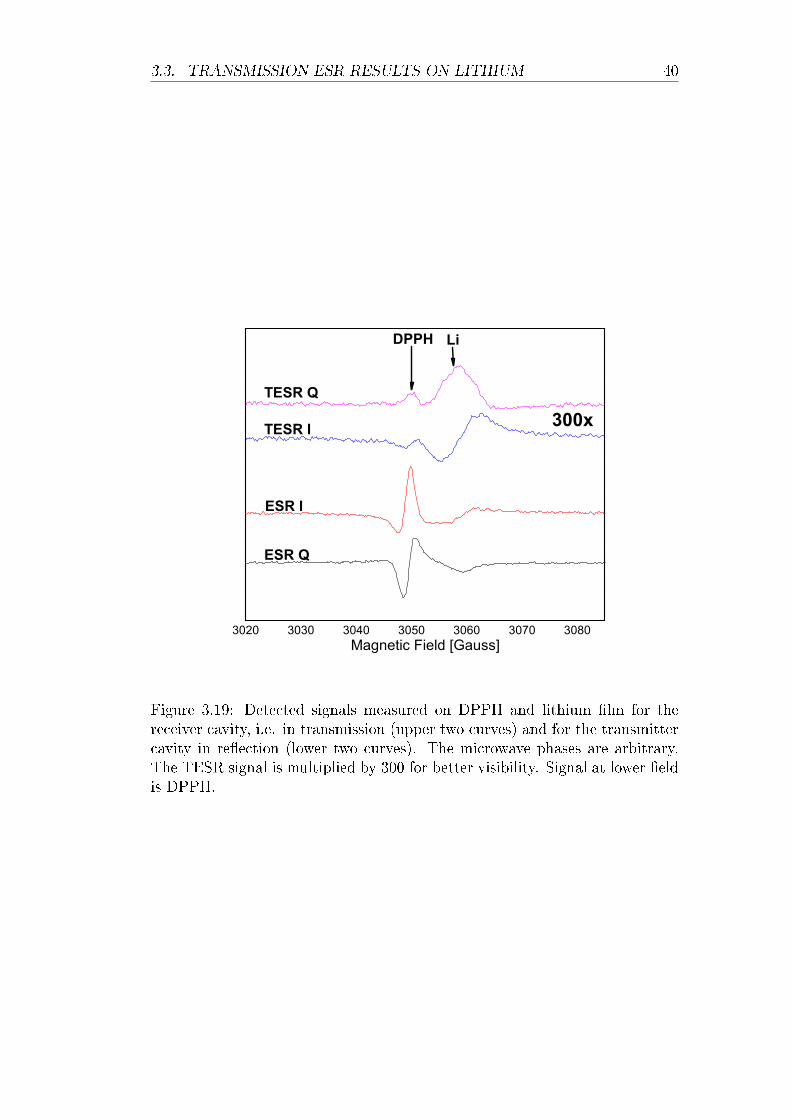
Although we measured the direct leakage with a modi�ed Cavity Sweepmethod, we performed additional control experiments. We placed a DPPHsample (less than 0.2 mg) next to the lithium sample which had about 150-200µm of thickness.The idea of the control experiment was to place an addi-tional ESR sample (DPPH) into the transmitter cavity. If we indeed observethe TESR of lithium, the ESR signal of the DPPH should be suppressed bythe amount of the leakage in the receiver cavity, whereas the TESR signal oflithium is expected to be much larger. The result is shown in Fig. 3.19.
The g-factor of DPPH is 2.0036, its resonance occurs at lower magnetic�elds. The g-factor of lithium is very close to the free electron ge-factor 2.0023,|ge − gLi|= 2 · 10−6 [19]. The linewidth is about 2 Gauss for both samples.We had to diminish the modulation amplitude because higher amplitude leadstotal overlap of the lines. Therefore we got very low intensity lithium signalsin re�ection. We measured 63 dB direct leakage and the DPPH intensitydecreased with this factor in transmission measurement. Lithium intensitydecreased with 38 dB. This experiment con�rms the earlier assignment, i.e.that we observe TESR of lithium. Some leakage is present but its magnitudeis controlled and its e�ect is taken into account.
3.3. TRANSMISSION ESR RESULTS ON LITHIUM 32
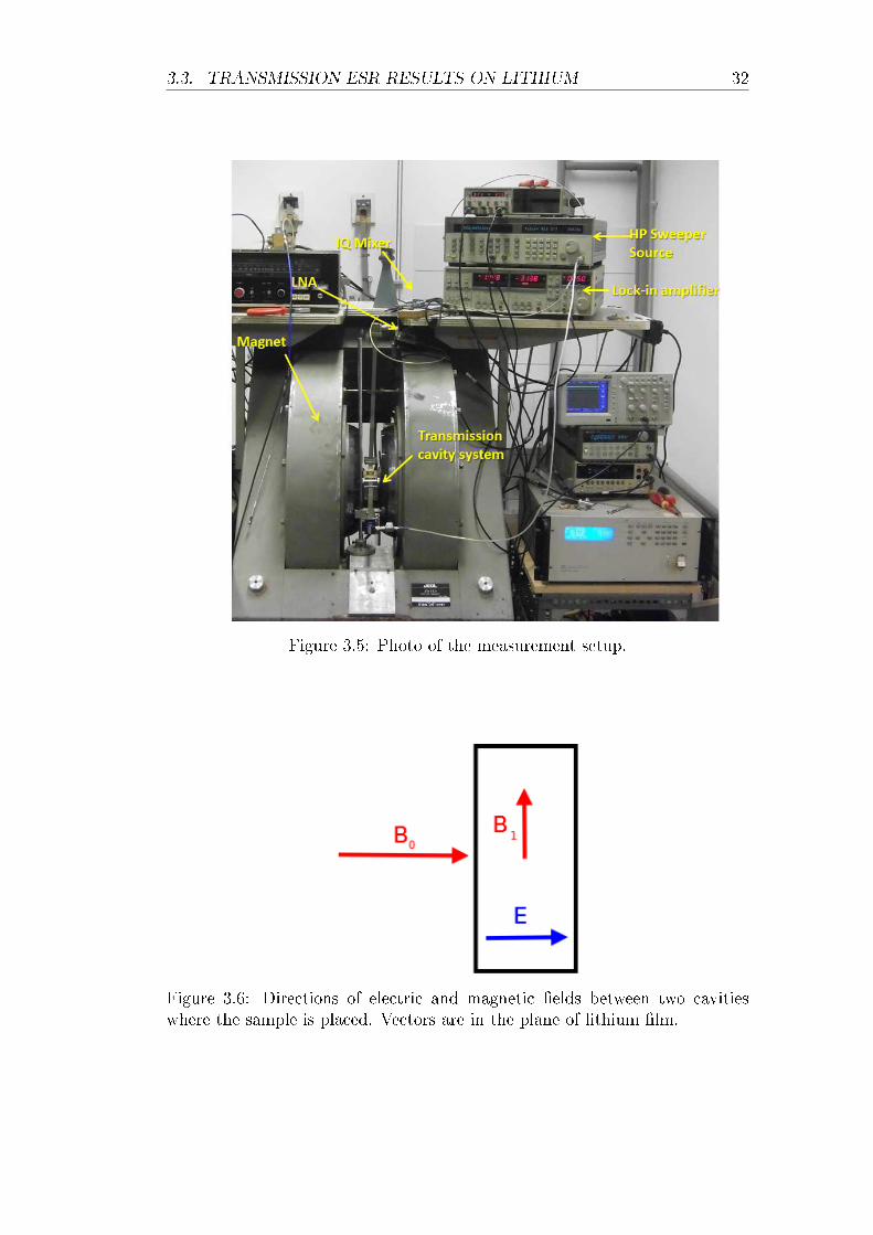
Figure 3.5: Photo of the measurement setup.
Figure 3.6: Directions of electric and magnetic �elds between two cavitieswhere the sample is placed. Vectors are in the plane of lithium �lm.
3.3. TRANSMISSION ESR RESULTS ON LITHIUM 33
Figure 3.7: Schematics of transmission cavity system.
Figure 3.8: The assembled transmission cavity system. Four holes on the topare for the modulation coil.
Figure 3.9: Sample and sample holder photographed inside the glovebox.
3.3. TRANSMISSION ESR RESULTS ON LITHIUM 34
HP SweeperSource
Directionalcoupler
IQ Mixer
LO
Transmittercavity
Receiver cavity
Magnet
Modulation coil
LNA
Lock-In
RF
I
Sample
B0
mod
1
Modulation signal
PC
B
B
Q
Figure 3.10: Schematics of TESR spectrometer
Lock-in
Duplexer
HP Sweeper source
Cavity
Detector
Figure 3.11: Schematics of Cavity Sweep arrangement
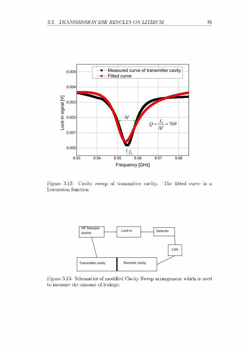
3.3. TRANSMISSION ESR RESULTS ON LITHIUM 35
9.53 9.54 9.55 9.56 9.57 9.58
0.000
0.001
0.002
0.003
0.004
0.005
Lo
ck-in
sig
nal [
V]
Frequency [GHz]
Measured curve of transmitter cavity Fitted curve
f
0f
7690
ffQ
Figure 3.12: Cavity sweep of transmitter cavity. The �tted curve is aLorentzian function
Lock-inHP Sweeper source
Detector
LNA
Transmitter cavity Receiver cavity
Figure 3.13: Schematics of modi�ed Cavity Sweep arrangement which is usedto measure the amount of leakage.
3.3. TRANSMISSION ESR RESULTS ON LITHIUM 36
9.50 9.52 9.54 9.56 9.58 9.60 9.62 9.64
0.000
0.001
0.002
0.003
0.004
0.005
0.006
Lock
-in s
igna
l [V
]
Frequency [GHz]
Peak of receiver cavityLeakage: 68.3 dB
Peak of transmitter cavityLeakage:79.9 dB
Figure 3.14: Crosstalk characterization with modi�ed Cavity Sweep.
HP SweeperSource
Directionalcoupler
IQ Mixer
LO
Transmittercavity
Receiver cavity
Magnet
Modulation coil
LNA
Lock-In
RF
I
Sample
B0
mod
1
Modulation signal
PC
B
B
Q
DuplexerAttenuators
Figure 3.15: Schematics of ESR spectrometer for reference signal measurement.
3.3. TRANSMISSION ESR RESULTS ON LITHIUM 37
3220 3230 3240 3250 3260 3270
TESR Q
TESR I
ESR Q
Magnetic field [Gauss]
100X
ESR I
Figure 3.16: Detected signals measured on 200µm �lm. The microwave phasesare random. TESR signal is multiplied by 100 for better visibility.
3.3. TRANSMISSION ESR RESULTS ON LITHIUM 38
0 100 200 300 400 500
-60
-40
-20
20lo
g(T/
R)
[dB
]
Sample thickness [ m]
Measured ratio Leakage Theoretical curve
Fitted line
Figure 3.17: Relative transmission signal and leakage with respect to the sam-ple thickness. The leakage is shown for comparison. A dashed curve shows thetheoretically expected relative TESR signal.
3.3. TRANSMISSION ESR RESULTS ON LITHIUM 39
3220 3230 3240 3250 3260 3270
-4.0x10⁻⁶
-3.0x10⁻⁶
-2.0x10⁻⁶
-1.0x10⁻⁶
0.0
1.0x10⁻⁶
2.0x10⁻⁶
3.0x10⁻⁶
ES
R s
igna
l [V
]
Magnetic field [Gauss]
ESR Q ESR I Hilbert transfrom of I
3220 3230 3240 3250 3260 3270
-3.0x10⁻⁶
-2.0x10⁻⁶
-1.0x10⁻⁶
0.0
1.0x10⁻⁶
2.0x10⁻⁶
3.0x10⁻⁶
TES
R s
igna
l [V
]
Magnetic Field [Gauss]
TESR Q TESR I Hilbert transform of I
Figure 3.18: The IQ mixer signals of the 200 µm sample and Hilbert trans-forms.
3.3. TRANSMISSION ESR RESULTS ON LITHIUM 40
3020 3030 3040 3050 3060 3070 3080
Magnetic Field [Gauss]
300x
ESR I
ESR Q
TESR Q
TESR I
DPPH Li
Figure 3.19: Detected signals measured on DPPH and lithium �lm for thereceiver cavity, i.e. in transmission (upper two curves) and for the transmittercavity in re�ection (lower two curves). The microwave phases are arbitrary.The TESR signal is multiplied by 300 for better visibility. Signal at lower �eldis DPPH.
Chapter 4
Summary
In this master thesis we summarized the technical and theoretical back-ground of electron spin resonance and profoundly understood the features ofdetected signals. We improved a transmission cavity system and an appropri-ate microwave circuit for detecting low level signals. Transmission electron spinresonance measurement was performed with modern devices and we showedhow e�ective they worked. The TESR spectroscopy has great opportunities inspintronics because the simultaneous detection of transport and spectroscopicphenomena is possible.
Future plans are to measure TESR on alkali doped graphite and to de-velop a pulsed ESR with this transmission cavity system with which even puregraphene becomes measurable.
41
Appendix A
Impedance matching
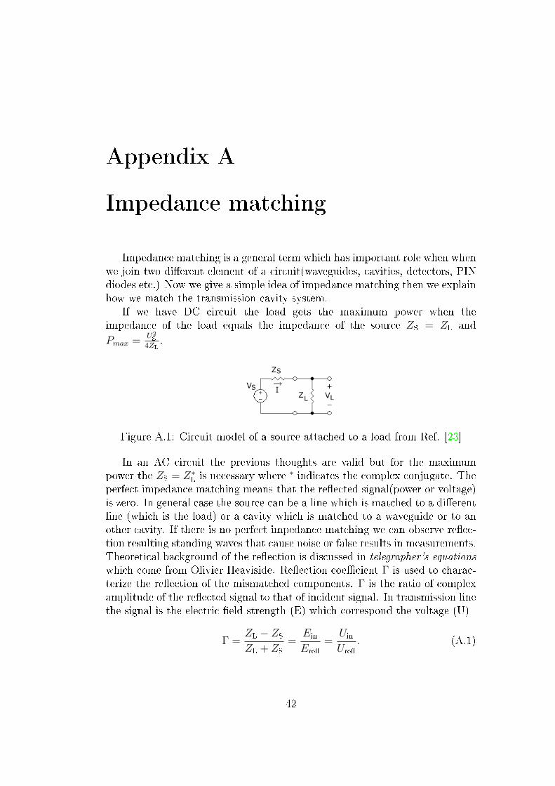
Impedance matching is a general term which has important role when whenwe join two di�erent element of a circuit(waveguides, cavities, detectors, PINdiodes etc.) Now we give a simple idea of impedance matching then we explainhow we match the transmission cavity system.
If we have DC circuit the load gets the maximum power when theimpedance of the load equals the impedance of the source ZS = ZL andPmax =
U2S
4ZL.
Figure A.1: Circuit model of a source attached to a load from Ref. [23]
In an AC circuit the previous thoughts are valid but for the maximumpower the ZS = Z∗L is necessary where ∗ indicates the complex conjugate. Theperfect impedance matching means that the re�ected signal(power or voltage)is zero. In general case the source can be a line which is matched to a di�erentline (which is the load) or a cavity which is matched to a waveguide or to another cavity. If there is no perfect impedance matching we can observe re�ec-tion resulting standing waves that cause noise or false results in measurements.Theoretical background of the re�ection is discussed in telegrapher's equations
which come from Olivier Heaviside. Re�ection coe�cient Γ is used to charac-terize the re�ection of the mismatched components. Γ is the ratio of complexamplitude of the re�ected signal to that of incident signal. In transmission linethe signal is the electric �eld strength (E) which correspond the voltage (U)
Γ =ZL − ZS
ZL + ZS
=Ein
Ere�
=UinUre�
. (A.1)
42
A.1. TESTS OF IMPEDANCE MATCHING 43
For a rectangular cavity the impedance is
Z =k√
µε√
k2 −(πa
)2(A.2)
where a is the length of longer side of the cross section of the waveguide,k = ω
√µε, µ and ε are the total permeability and permittivity respectively, ω
is the cavity resonance angular frequency [21, 22].Every TESR measurement on di�erent samples requires a reconstruction of
the cavity system. We observed that the resonance frequency of the transmitterand receiver cavity had di�erent values from experiment to experiment. Thise�ect was probably related to the way the cavity wall-end copper plate wasmounted. Now we show that the di�erent resonance frequency and impedancedoes not cause signi�cant e�ect on the experiments. Table A.1 shows that
Sample size [µm] ∆f [MHz] Γ90 30.619 0.001336150 27.101 0.001265200 250.638 0.01088480 378.43 0.01647
Table A.1: Re�ection coe�cient with respect to the frequency di�erence be-tween transmitter and receiver cavity.
re�ection coe�cient much less than unity therefore it has no e�ect on thetransmission ESR signal. The lithium sample behaves as an radiant source. Inthe receiver cavity the di�using electrons are able to build up the microwave�eld with the resonance frequency of the transmitter cavity.
A.1 Tests of impedance matching
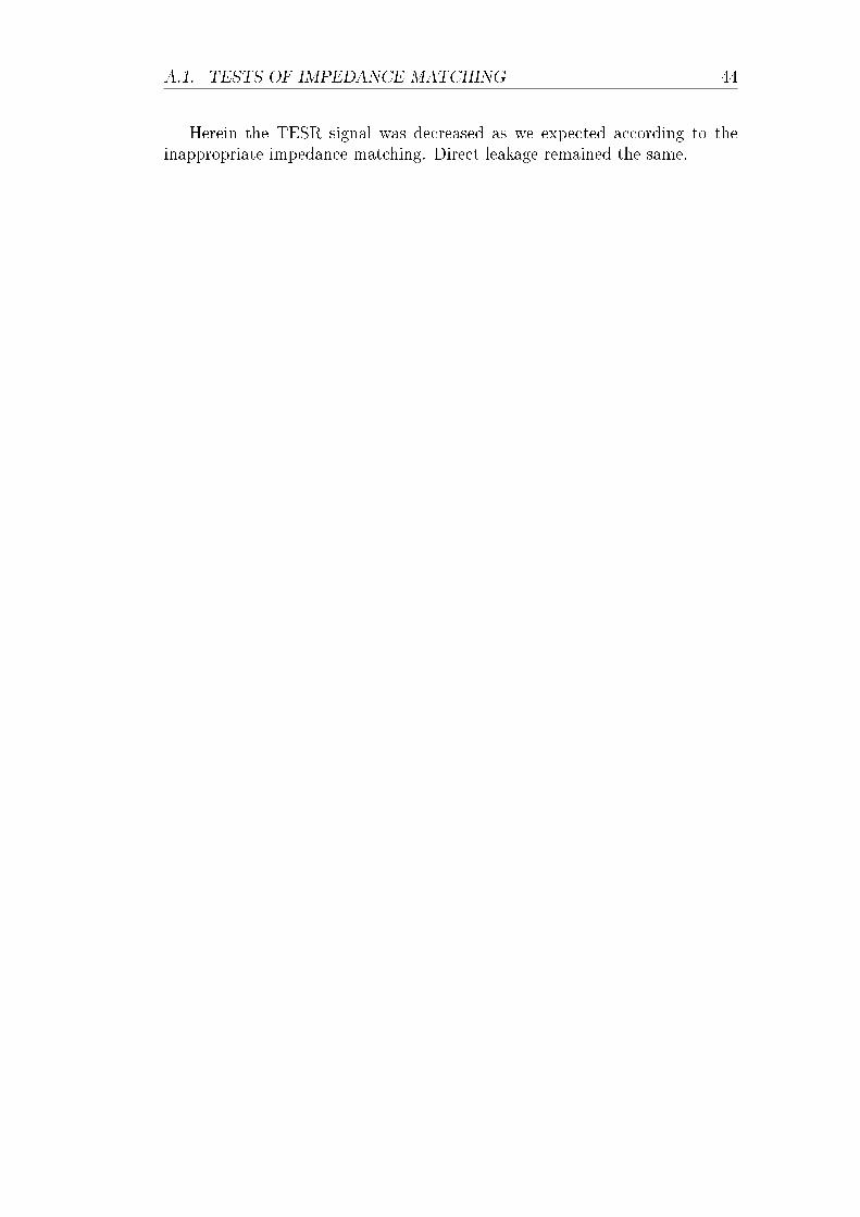
We made a tunable receiver cavity1 and we examined the leakage of thetransmission cavity system when only a holeless copper plate was placed be-tween the cavities.
Fig. A.2 shows that the leakage power add up when the two cavities arebrought to a common resonance frequency. This also means that a slightdetuning between the two cavities do not a�ect neither the leakage nor theTESR signal.
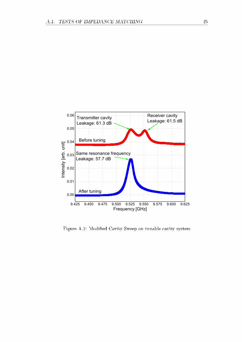
In other experiment we removed the enclosing copper plate of the re-ceiver cavity. The receiver cavity and the transmitter waveguide are totallyimpedance mismatched in this case. A 80 µm thick lithium �lm was placedafter the transmitter cavity. The result is shown in Fig.A.3.
1This construction was not properly air tight so it had a limited use in the TESR exper-iments.
A.1. TESTS OF IMPEDANCE MATCHING 44
Herein the TESR signal was decreased as we expected according to theinappropriate impedance matching. Direct leakage remained the same.
A.1. TESTS OF IMPEDANCE MATCHING 45
9.425 9.450 9.475 9.500 9.525 9.550 9.575 9.600 9.625
0.00
0.01
0.02
0.03
0.04
0.05
0.06
Inte
nsity
[arb
. uni
t]
Frequency [GHz]
Transmitter cavityLeakage: 61.3 dB
Receiver cavityLeakage: 61.5 dB
Same resonance frequencyLeakage: 57.7 dB
Before tuning
After tuning
Figure A.2: Modi�ed Cavity Sweep on tunable cavity system
A.1. TESTS OF IMPEDANCE MATCHING 46
0 100 200 300 400 500
-60
-40
-20
20lo
g(T/
R)
[dB
]
Sample thickness [ m]
Measured ratio Leakage Theoretical curve
Fitted line
Without receiver cavity
Figure A.3: The original measurement results with the results of one cavitymeasurement.
Appendix B
Technical details of the TESR
spectrometer
B.1 Cavity parameters
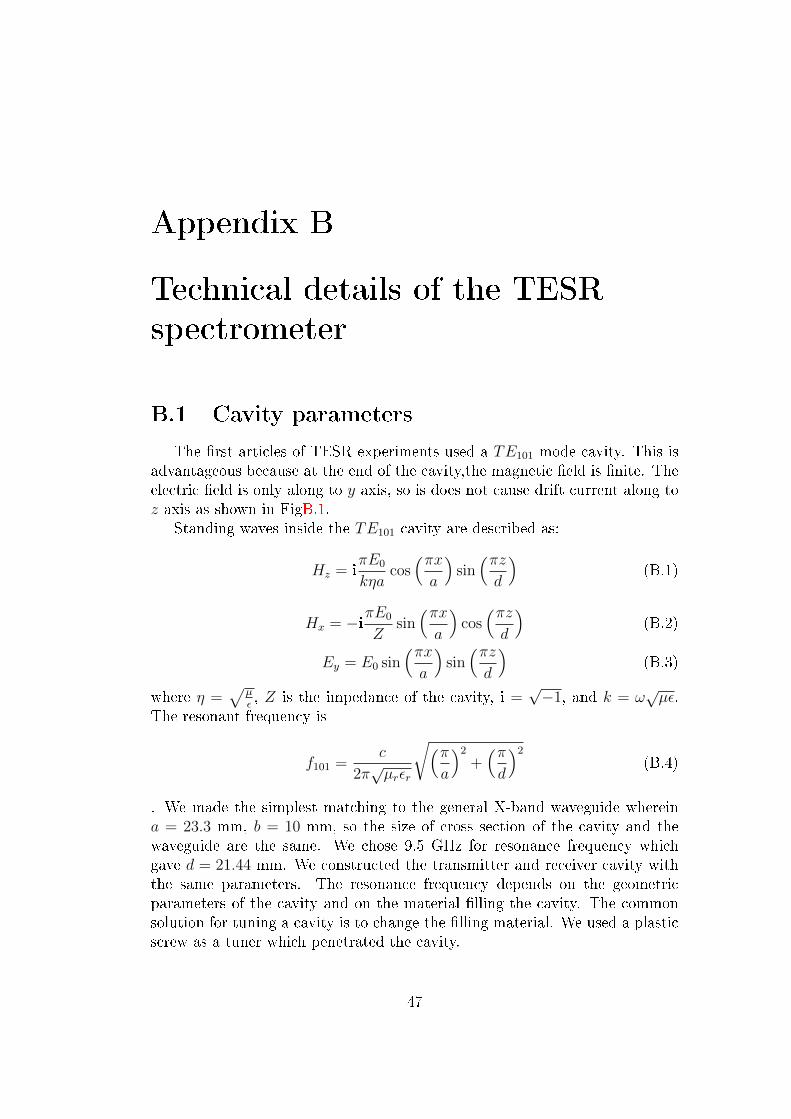
The �rst articles of TESR experiments used a TE101 mode cavity. This isadvantageous because at the end of the cavity,the magnetic �eld is �nite. Theelectric �eld is only along to y axis, so is does not cause drift current along toz axis as shown in FigB.1.
Standing waves inside the TE101 cavity are described as:
Hz = iπE0
kηacos(πxa
)sin(πzd
)(B.1)
Hx = −iπE0
Zsin(πxa
)cos(πzd
)(B.2)
Ey = E0 sin(πxa
)sin(πzd
)(B.3)
where η =√
µε, Z is the impedance of the cavity, i =
√−1, and k = ω
√µε.
The resonant frequency is
f101 =c
2π√µrεr
√(πa
)2
+(πd
)2
(B.4)
. We made the simplest matching to the general X-band waveguide whereina = 23.3 mm, b = 10 mm, so the size of cross section of the cavity and thewaveguide are the same. We chose 9.5 GHz for resonance frequency whichgave d = 21.44 mm. We constructed the transmitter and receiver cavity withthe same parameters. The resonance frequency depends on the geometricparameters of the cavity and on the material �lling the cavity. The commonsolution for tuning a cavity is to change the �lling material. We used a plasticscrew as a tuner which penetrated the cavity.
47
B.2. TESR EXPERIMENT PARAMETERS 48
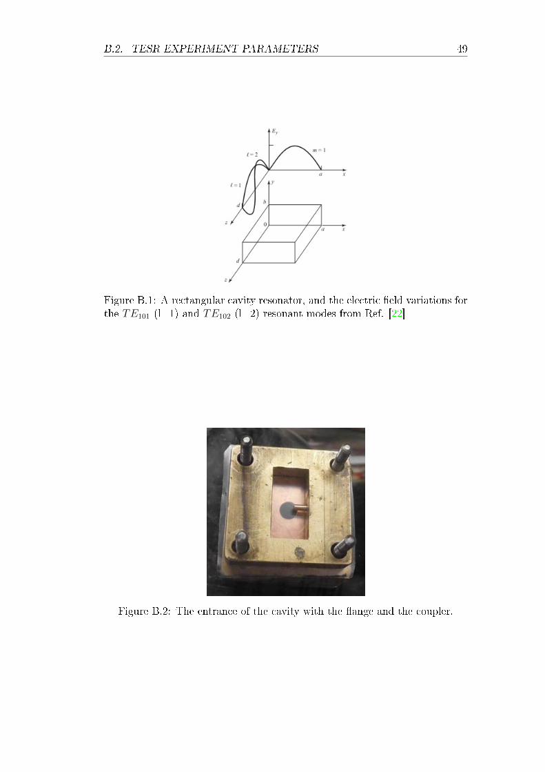
To obtain critical coupling which means perfect impedance matching, weput a metal coupler into the �ange which presses the o-ring and the cavity asshown in Fig. B.2.
Several experiments showed that the most e�ective coupling is reachedwhen the coupler is parallel to the electric �eld, and the coupler is placedwhere the electric �eld has maximum value (x = a
2).
The best size of the hole of enclosing copper plate was determined byexperimental way. We closed the cavity with di�erent plates which had 3-10 mm diameter holes and we performed Cavity Sweep. We chose the platewhich had diameter 6.5 mm because it gave critical coupling and high Q-factor.The hole of the sample holder had 6.5 mm diameter as well.
B.2 TESR experiment parameters
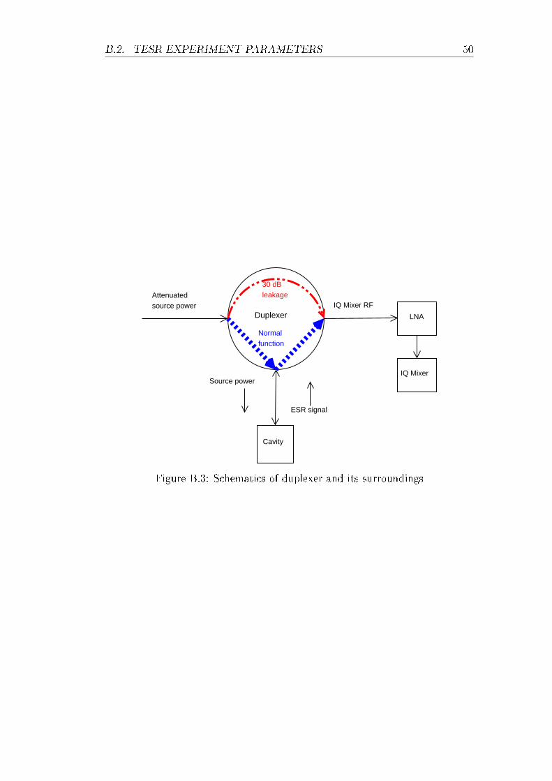
The output of the microwave source was always 20 dBm. The re�ectionESR measurement was performed with at least 40 dB attenuation of the sourcepower. Less attenuation caused the saturation of the IQ mixer. The reason isthe imperfection of the duplexer: it is a circulator which has isolation of about30 dB, i.e. some of the exciting power always reaches the mixer as shown inFigB.3.
If we used 20 dBm power, the leakage signal at RF port would be -30dBm but the LNA ampli�es 36 dB, therefore 6 dBm is the RF signal from theleakage. In general, a mixer is saturated if the RF port power exceeds 10 dBless than the work point power at the LO. The IQ mixer works with 10 dBmLO, so 6 dBm RF is too high, so the usage of attenuators is reasonable.
B.2. TESR EXPERIMENT PARAMETERS 49
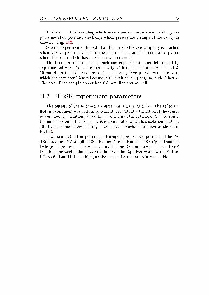
Figure B.1: A rectangular cavity resonator, and the electric �eld variations forthe TE101 (l=1) and TE102 (l=2) resonant modes from Ref. [22]
Figure B.2: The entrance of the cavity with the �ange and the coupler.
B.2. TESR EXPERIMENT PARAMETERS 50
Cavity
Source power
ESR signal
Attenuated source power
30 dBleakage
Normalfunction
DuplexerIQ Mixer RF
LNA
IQ Mixer
Figure B.3: Schematics of duplexer and its surroundings
Appendix C
Advantage of Low Noise
Ampli�ers
Attaining the best signal to noise ratio (SNR) is the priority in any branchesof measurement science. Now we give a short explanation about general lownoise measurement and the bene�t of the use of LNAs according to Ref. [24,25].
In 1942, Harald T. Friis, working in Bell Labs, developed the theory of"noise �gure" (NF) to calculate the signal to noise ratio at the output of acomplex receiver chain. De�nition of NF of a device is
NF = 10 log10
(SNRin
SNRout
)= 10 log10(F ) (C.1)
where SNRout and SNRin are the output and input signal to noise power ratios,respectively. Noise �gure is often used in microwave engineering but the noisefactor is used for noise calculation. The noise factor is F = SNRin
SNRout. The SNR
is the most convenient way of quantifying how much thermal noise the receiveradds to the signal. F is a measure of how the SNR is reduced by a device.The noise factor is correlated with the thermal noise power PThermal = kBT∆fwhich is -174 dBm at room temperature with 1 Hz bandwidth (where k_B)is the Boltzmann constant). Noise factor expresses how many times morenoise we obtain at the output of a device. Depending on where devices arepositioned in a complex receiver chain, the individual noise factors will havedi�erent e�ects on the overall noise, according to Friis's equation which givesthe resultant noise factor of the receiver chain as:
F = F1 +F2 − 1
G1
+F3 − 1
G1G2
+F4 − 1
G1G2G3
+ · · ·+ Fn − 1
G1G2G3 · · ·Gn−1
(C.2)
where Gi and Fi are the available power gain and noise factor, respectively,of the i-th stage, and n is the number of stages. The �rst ampli�er in thechain has the most signi�cant e�ect on the total noise �gure than any otherampli�er in the chain. The lowest noise �gure ampli�er has to go �rst in a line
51
52
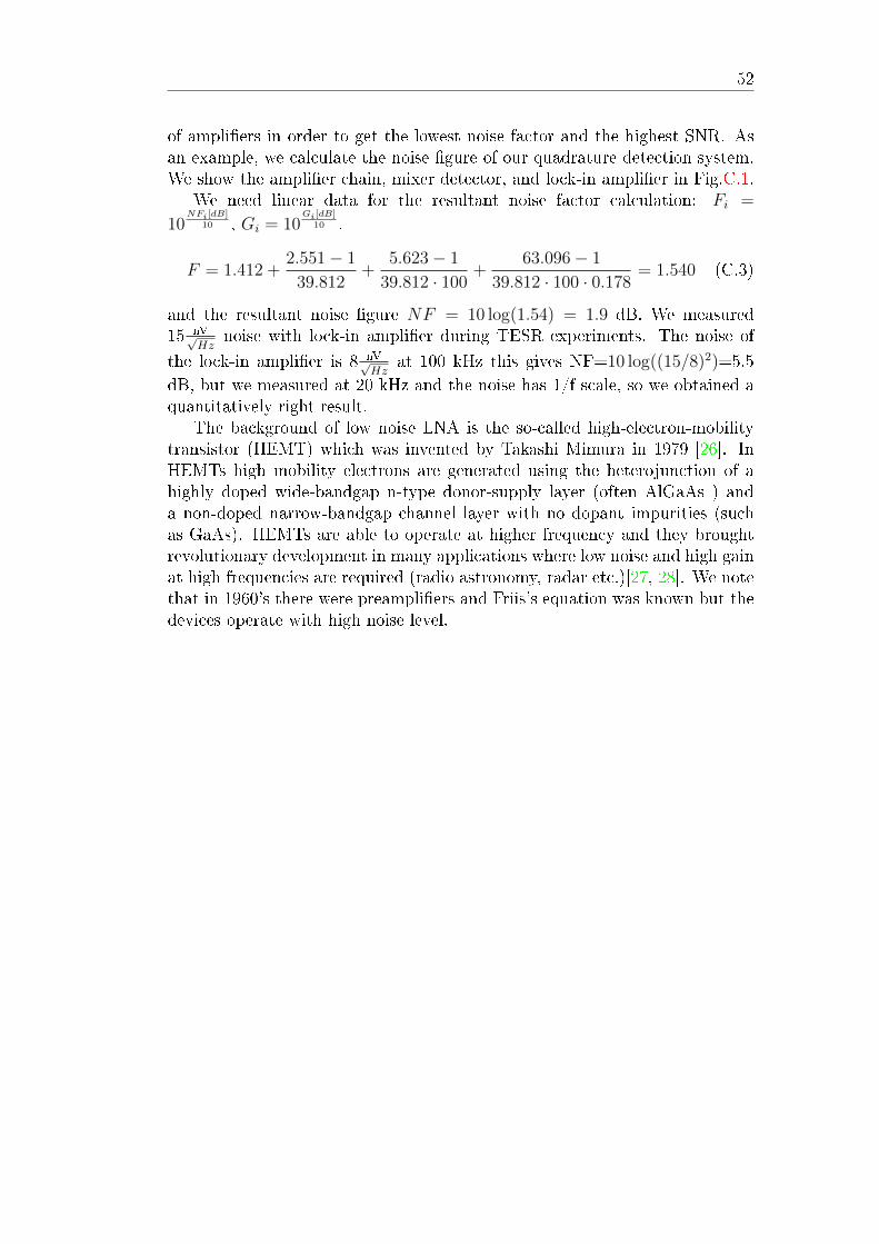
of ampli�ers in order to get the lowest noise factor and the highest SNR. Asan example, we calculate the noise �gure of our quadrature detection system.We show the ampli�er chain, mixer detector, and lock-in ampli�er in Fig.C.1.
We need linear data for the resultant noise factor calculation: Fi =
10NFi[dB]
10 , Gi = 10Gi[dB]
10 .
F = 1.412 +2.551− 1
39.812+
5.623− 1
39.812 · 100+
63.096− 1
39.812 · 100 · 0.178= 1.540 (C.3)
and the resultant noise �gure NF = 10 log(1.54) = 1.9 dB. We measured15 nV√
Hznoise with lock-in ampli�er during TESR experiments. The noise of
the lock-in ampli�er is 8 nV√Hz
at 100 kHz this gives NF=10 log((15/8)2)=5.5dB, but we measured at 20 kHz and the noise has 1/f scale, so we obtained aquantitatively right result.
The background of low noise LNA is the so-called high-electron-mobilitytransistor (HEMT) which was invented by Takashi Mimura in 1979 [26]. InHEMTs high mobility electrons are generated using the heterojunction of ahighly doped wide-bandgap n-type donor-supply layer (often AlGaAs ) anda non-doped narrow-bandgap channel layer with no dopant impurities (suchas GaAs). HEMTs are able to operate at higher frequency and they broughtrevolutionary development in many applications where low noise and high gainat high frequencies are required (radio astronomy, radar etc.)[27, 28]. We notethat in 1960's there were preampli�ers and Friis's equation was known but thedevices operate with high noise level.
53
3.2.1. 4.
LNA 1. LNA 2. IQ Mixer Lock-in
NF=1.5 dB
G=16 dB
NF=4 dB
G=20 dB
NF=7.5 dB
G=-7.5 dB
NF=18 dB
G=-18 dB
Figure C.1: Schematics of receiver chain.
Appendix D
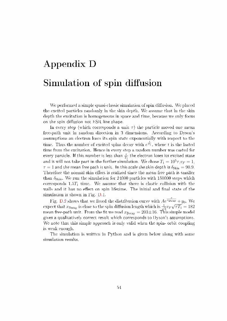
Simulation of spin di�usion
We performed a simple quasi-classic simulation of spin di�usion. We placedthe excited particles randomly in the skin depth. We assume that in the skindepth the excitation is homogeneous in space and time, because we only focuson the spin di�usion not ESR line shape.
In every step (which corresponds a unit τ) the particle moved one meanfree-path unit in random direction in 3 dimensions. According to Dyson'sassumptions an electron loses its spin state exponentially with respect to thetime. Thus the number of excited spins decay with e
tT1 , where t is the lasted
time from the excitation. Hence in every step a random number was casted forevery particle. If this number is less than τ
T1the electron loses its excited state
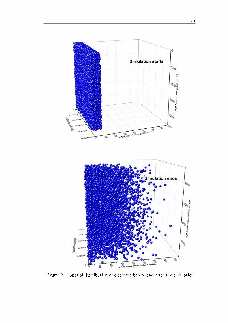
and it will not take part in the further simulation. We chose T1 = 105τ ,vF = 1,τ = 1 and the mean free path is unit. In this scale the skin depth is δSkin = 90.9.Therefore the normal skin e�ect is realized since the mean free path is smallerthan δSkin. We run the simulation for 24000 particles with 150000 steps whichcorresponds 1.5T1 time. We assume that there is elastic collision with thewalls and it has no e�ect on spin lifetime. The initial and �nal state of thesimulation is shown in Fig. D.1.
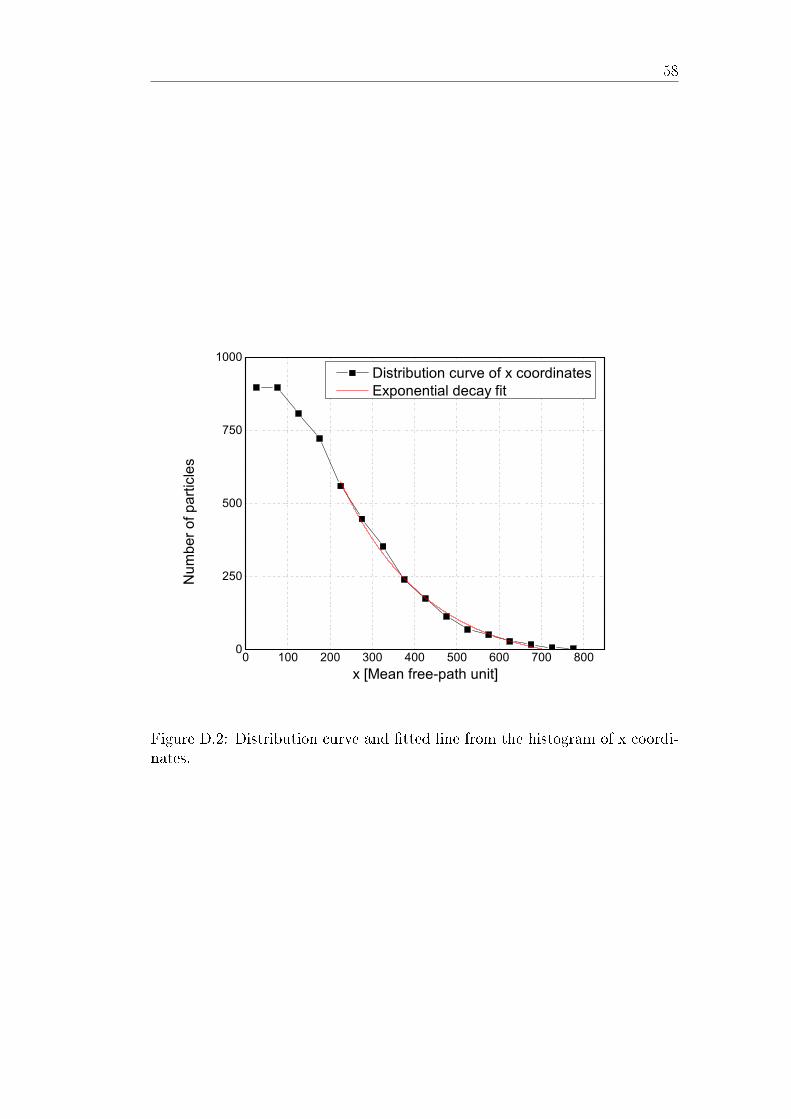
Fig. D.2 shows that we �tted the distribution curve with Aex
xDecay +y0. Weexpect that xDecay is close to the spin di�usion length which is 1√
3vF√τT1 = 182
mean free-path unit. From the �t we read xDecay = 203±16. This simple modelgives a qualitatively correct result which corresponds to Dyson's assumptions.We note that this simple approach is only valid when the spin- orbit couplingis weak enough.
The simulation is written in Python and is given below along with somesimulation results.
54
# coding=utf-8
from random import randint
import timeit
import math
FREE_PATH = 1
number_of_electrons =24000electrons = []
class box:def __init__(self,origo = [],diagonal_point = []):
self.origo = origo
self.diagonal_point = diagonal_point
def return_random(self): # choose random point in the box between origo and diagonal_point
return [uniform(self.origo[0],self.diagonal_point[0]),uniform(self.origo[1],self.diagonal_point[1]),uniform(self.origo[2],self.diagonal_point[2])]
class e_part:def __init__(self, spin, coordinate = []):
self.coordinate = coordinate
self.spin = spin
def move_step(self,inbox = box([0, 0, 0],[10, 10, 10])):dz_coord = uniform(-FREE_PATH,FREE_PATH)phi = uniform(0,1)dx_coord = math.sqrt((FREE_PATH*FREE_PATH)-dz_coord*dz_coord)* math.cos(2*math.pi*phi)dy_coord = math.sqrt((FREE_PATH*FREE_PATH)-dz_coord*dz_coord)* math.sin(2*math.pi*phi)self.coordinate[0] = self.coordinate[0] + dx_coord
self.coordinate[1] = self.coordinate[1] + dy_coord
self.coordinate[2] = self.coordinate[2] + dz_coord
#print("collisions with walls")
#X collisions
if(self.coordinate[0] < inbox.origo[0]):self.coordinate[0] = 2*inbox.origo[0] - self.coordinate[0]
if(self.coordinate[0] > inbox.diagonal_point[0]):self.coordinate[0] = 2*inbox.diagonal_point[0] - self.coordinate[0]
#Y collisions
if(self.coordinate[1] < inbox.origo[1]):self.coordinate[1] = 2*inbox.origo[1] - self.coordinate[1]
if(self.coordinate[1] > inbox.diagonal_point[1]):self.coordinate[1] = 2*inbox.diagonal_point[1] - self.coordinate[1]
#Z collisions
if(self.coordinate[2] < inbox.origo[2]):self.coordinate[2] = 2*inbox.origo[2] - self.coordinate[2]
if(self.coordinate[2] > inbox.diagonal_point[2]):
-1-
self.coordinate[2] = 2*inbox.diagonal_point[2] - self.coordinate[2]
def check_in_box (self,inbox = box([0,0,0],[10,10,10])):return ((inbox.origo[0]< self.coordinate[0]< inbox.diagonal_point[0] )and (inbox.origo[1]< self.coordinate[1]< inbox.diagonal_point[1])and (inbox.origo[2]< self.coordinate[2]<inbox.diagonal_point[2]))
def main():f = open('sim.txt','w')start = timeit.default_timer()sum = 0
start_box = box([0,0,0],[90.9,909090,909090])end_box = box([2636,0,0],[2727,909090,909090])full_box = box([0,0,0],[2727,909090,909090])electrons = [] #create a list
for count in range(1,number_of_electrons):electron_item = e_part(1,start_box.return_random())electron_item.attr = count
electrons.append(electron_item)for t in range(1,150000): ##about 1.5*T1 time
for electron in electrons:if (uniform(0,1000000)<10 ):
electrons.remove(electron)
electron.move_step(full_box)
for electron in electrons:print electron.coordinate[0] #
if(electron.check_in_box(full_box)):f.write(str(t)) #write t and coordinates when an electron lives
f.write('\t')f.write(str(electron.coordinate[0]))f.write('\t')f.write(str(electron.coordinate[1]))f.write('\t')f.write(str(electron.coordinate[2]))f.write('\n')sum += 1
print sum
f.close()stop = timeit.default_timer()print "runtime:" + str(stop - start )
if __name__ == "__main__": main()
-2-
57
Figure D.1: Spatial distribution of electrons before and after the simulation
58
0 100 200 300 400 500 600 700 8000
250
500
750
1000
Num
ber o
f par
ticle
s
x [Mean free-path unit]
Distribution curve of x coordinates Exponential decay fit
Figure D.2: Distribution curve and �tted line from the histogram of x coordi-nates.
Bibliography
[1] Y. K. Zavoisky, Paramagnetic Absorption in Perpendicular and ParallelFields for Salts, Solutions and Metals, PhD thesis, Kazan State University,1944
[2] F. Bloch, �Nuclear induction",Phys. Rev., vol. 70, pp. 460�474, Oct 1946.
[3] I. �uti¢, J. Fabian, and S. D. Sarma, �Spintronics: Fundamentals andapplications,� Rev. Mod. Phys., vol. 76, pp. 323�410, 2004.
[4] F. J. Dyson, �Electron Spin Resonance Absorption in Metals. II. Theoryof Electron Di�usion and the Skin E�ect,�Physical Review, vol. 98, p. 349,1955.
[5] G. Feher and A. F. Kip, �Electron Spin Resonance Absorption in Metals.I. Experimental,� Physical Review, vol. 98, p. 337, 1955.
[6] M. Ya.Azbel', V.I. Gerasimenko, and I. M.Lifshitz, Zh. Eksperim. i. Teor.Fiz.32, 1212(1957) [translation: Soviet Phys. �JETP5, 986(1957)
[7] R.B. Lewis and T.R. Carver, Conduction electron spin resonance in lithiumPhys. Rev. Letters 12, 693(1964)
[8] T. H. Wilmshurst: Electron Spin Resonance Spectrometers (Monographson electron spin resonance) London : Hilger, 1967.
[9] http://www.ittc.ku.edu/ jstiles/622/handouts/Mixer%20Conversion%20Loss.pdf2015.05.15.
[10] http://www.markimicrowave.com/blog/2013/06/iq-image-reject-and-single-sideband-mixers/ 2015.05.16.
[11] N. S. VanderVen and R.T. Schumacher, Resonant transmission of mi-crowave power through "thick" �lms of lithium metal Phys. Rev. Letters12, 695(1964)
[12] Jerome I. Kaplan, Application of the Di�usion-Modi�ed Bloch Equationto Electron Spin Resonance in Ordinary and Ferromagnetic Metals, Phys.Rev. 115, 575 (1959)
59
BIBLIOGRAPHY 60
[13] R. de L. Kronig, "On the theory of the dispersion of X-rays". J. Opt. Soc.Am. 12: 547�557 (1926)
[14] H.A. Kramers, "La di�usion de la lumiere par les atomes". Atti Cong.Intern. Fisici (1927)
[15] Hilbert David Grundzüge einer allgemeinen Theorie der linearen Integral-gleichungen, Chelsea Pub. Co. (1953)
[16] B.V. Khvedelidze, "Hilbert transform", in Hazewinkel, Michiel, Encyclo-pedia of Mathematics, Springer (2001)
[17] András Jánossy, Resonant and nonresonant conduction-electron-spintransmission in normal metals, Phys.Rev. B 21,3793 (1970)
[18] Pandey, J.N. (1996), The Hilbert transform of Schwartz distributions andapplications, Wiley-Interscience
[19] R. J. Pressley and H. L. Berk, g Factor of Conduction Electrons in MetallicLithium, Phys. Rev. 140. A1207,(1965)
[20] Charles P. Poole, Electron Spin Resonance � A Comprehensive Treatiseon Experimental Techniques, Interscience Publishers 1967
[21] John D. Kraus, Electromagnetics, McGraw-Hill Companies 1992,
[22] David Pozar, Microwave Engineering, John Wiley & Sons, Inc.
[23] http://en.wikipedia.org/wiki/Impedance_matching 2015.05.20.
[24] J.D. Kraus, Radio Astronomy, McGraw-Hill, 1966
[25] http://www.microwaves101.com/encyclopedias/noise-�gure 2015.05.20.
[26] Takashi Mimura: 'The Early History of the High Electron Mobility Tran-sistor (HEMT)',IEEE TRANSACTIONS ON MICROWAVE THEORYAND TECHNIQUES, VOL. 50, NO. 3, MARCH 2002
[27] http://www.semiconductor-today.com/news_items/2014/OCT/NORTHROP-GRUMMAN_311014.shtml 2015.05.18.
[28] http://en.wikipedia.org/wiki/High-electron-mobility_transistor#cite_note-2 2015.05.15.
[29] N. Tombros, C. Józsa, M. Popinciuc, H. T. Jonkman, and B. J. van Wees,Nature (London) 448, 571 (2007).
[30] N. Tombros, S. Tanabe, A. Veligura, C. Jozsa, M. Popinciuc, H. T.Jonkman, and B. J. van Wees Phys. Rev. Lett. 101, 046601