UCD CENTRE FOR ECONOMIC RESEARCH

WORKING PAPER SERIES

2010

The Economic Impact of the Little Ice Age

Morgan Kelly and Cormac Ó Gráda, University College Dublin

WP10/14

April 2010

UCD SCHOOL OF ECONOMICS UNIVERSITY COLLEGE DUBLIN

BELFIELD DUBLIN 4

The Economic Impact of the Little Ice Age.

Morgan Kelly and Cormac Ó Gráda∗

April 16, 2010

Abstract

We investigate by how much the Little Ice Age reduced the harvests on

which pre-industrial Europeans relied for survival. We find that weather

strongly affected crop yields, but can find little evidence that western Eu-

rope experienced long swings or structural breaks in climate. Instead, an-

nual summer temperature reconstructions between the fourteenth and twen-

tieth centuries behave as almost independent draws from a distribution with

a constant mean but time varying volatility; while winter temperatures be-

have similarly until the late nineteenth century when they rise markedly,

consistent with anthropogenic global warming. Our results suggest that the

existing consensus about a Little Ice Age in western Europe stems from a

Slutsky effect, where the standard climatological practice of smoothing data

prior to analysis induces spurious cyclicality in uncorrelated data.

The Little Ice Age is conventionally viewed as a major event of climatic history,with episodes of deep cold causing glaciers to advance, the Thames in Londonto freeze, and the Norse colonies in Greenland to perish. The consensus among

∗School of Economics, University College Dublin. This research was undertaken as part ofthe HI-POD (Historical Patterns of Development and Underdevelopment: Origins and Persistenceof the Great Divergence) Project supported by the European Commission’s 7th Framework Pro-gramme for Research.

1

climatologists is that the Northern Hemisphere above the tropics experienced sus-tained episodes of reduced temperatures between the fifteenth and nineteenth cen-turies, with particularly marked falls in Europe (Mann 2002, Matthews and Briffa2005, Mann et al. 2009. We investigate the economic cost of the Little Ice Age:by how much did the worse climate of the period reduce the harvests on whichpre-industrial Europeans relied for survival? Although we find that crop yieldswere strongly affected by weather, we find little evidence of variation in Euro-pean climate: the distribution of summer temperatures appears unchanged be-tween the fourteenth and twentieth centuries, while winter temperatures remainconstant until the late nineteenth century, after which they rise markedly, consis-tent with global warming.1

To analyse how weather affected harvests we use data on cereal yields onover 100 English manors between 1211 and 1450 compiled by Campbell (2007).Manors belonging to religious and other institutions kept detailed annual accountsthat give the most accurate information on harvest yields, outside China, beforethe late nineteenth century. We find that two weather reconstructions have strongexplanatory power for annual harvests: Low Countries summer temperatures, andthe thickness of annual growth rings of Irish oaks (which correlate with summerprecipitation).

A one degree Celsius fall in summer temperature reduced yields of wheat byaround 5 per cent, and a one standard deviation rise in summer rainfall reducedyields by around 10 per cent. While yields of the cheaper spring grains on whichordinary people subsisted were less affected by weather, their prices closely fol-lowed yields of wheat, the main commercial crop. Epidemic diseases after badharvests were deadly at all levels of society: a 10 per cent fall in real wages causedby a bad harvest resulted in a 7 per cent rise in mortality among both unfree tenants

1Strictly speaking, our results give an upper bound for the economic cost of the Little Ice Age,that assumes that people did not shift to cultivating more weather resistant crops during episodesof climatic deterioration. However, because the upper bound for the cost of the Little Ice Ageappears to be zero, we did not attempt to refine our estimate.

2

Deg

rees

C

15.8

16.0

16.2

16.4

16.6

1300

1320

1340

1360

1380

1400

1420

1440

1460

1480

1500

1520

1540

1560

1580

1600

1620

1640

1660

1680

1700

1720

1740

1760

1780

1800

1820

1840

1860

1880

1900

1920

1940

1960

1980

2000

Deg

rees

C

14

15

16

17

18

1300

1320

1340

1360

1380

1400

1420

1440

1460

1480

1500

1520

1540

1560

1580

1600

1620

1640

1660

1680

1700

1720

1740

1760

1780

1800

1820

1840

1860

1880

1900

1920

1940

1960

1980

2000

Deg

rees

C

14

15

16

17

18

● ●

●

●

●

●

●●●

●●

●

●

●●

●

●

●

●

●

●

●●

●

C14.H

1

C14.H

2

C15.H

1

C15.H

2

C16.H

1

C16.H

2

C17.H

1

C17.H

2

C18.H

1

C18.H

2

C19.H

1

C19.H

2

C20.H

1

C20.H

2

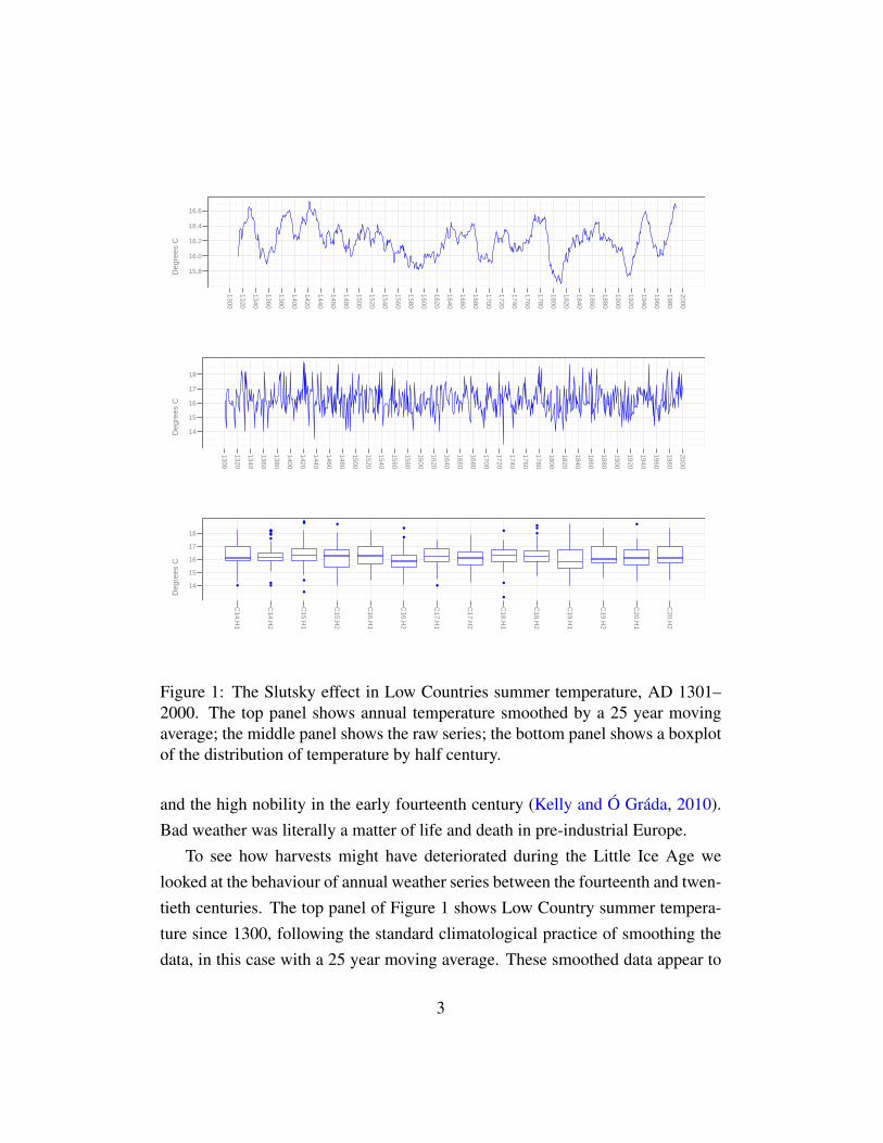
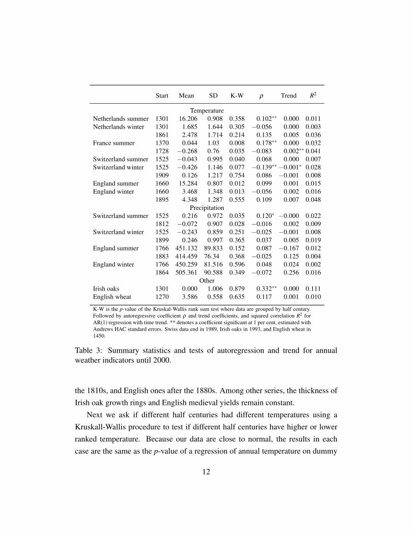
Figure 1: The Slutsky effect in Low Countries summer temperature, AD 1301–2000. The top panel shows annual temperature smoothed by a 25 year movingaverage; the middle panel shows the raw series; the bottom panel shows a boxplotof the distribution of temperature by half century.

and the high nobility in the early fourteenth century (Kelly and Ó Gráda, 2010).Bad weather was literally a matter of life and death in pre-industrial Europe.

To see how harvests might have deteriorated during the Little Ice Age welooked at the behaviour of annual weather series between the fourteenth and twen-tieth centuries. The top panel of Figure 1 shows Low Country summer tempera-ture since 1300, following the standard climatological practice of smoothing thedata, in this case with a 25 year moving average. These smoothed data appear to

3

show a cooling trend from the mid-fifteenth to the early nineteenth centuries, withmarked cold episodes in the late sixteenth, late seventeenth, and early nineteenthcenturies, consistent with the consensus about a Little Ice Age.

However, when we look instead at the unsmoothed data, in the middle panelof Figure 1, the impression is one of randomness without structural breaks, cyclesor trends, but with episodes of low and high volatility. Standard statistical testsconfirm that this is the case. The bottom panel shows a boxplot of the distributionof temperature by half century, which shows how median summer temperaturehas fluctuated by a fraction of a degree between 1301 and 2000.

This low autocorrelation in annual levels but strong autocorrelation in varianceis not an idiosyncrasy of this one weather series, but is common to most widelyused long-run reconstructions of western European weather. In Section 3 we lookat the time series behaviour of the Low Countries temperature series, and alsohistorical temperature estimates for Switzerland, France and England; Irish oaks,and rainfall estimates for Switzerland and England.

In nearly all cases we find little dependence in temperature or rainfall betweenone year and the next, and no evidence of trends. Annual summer temperature inEurope between the fourteenth and twentieth centuries appears as almost indepen-dent draws from a distribution with a constant mean but a variance that changesthrough time. Similarly the distribution of rainfall and winter temperature appearsconstant until the late nineteenth century, but then changes markedly. Instrumen-tal records of temperature from European cities since the eighteenth century tell asimilar story.

In summary, then, annual weather series do not show cycles or structuralbreaks consistent with a Little Ice Age. Instead their levels show weak auto-correlation while their variances show strong autoregression. This pattern closelyresembles the behaviour of a typical financial return series.

That our findings run counter to the existing consensus of a European LittleIce Age reflects our statistical approach. We analyse unsmoothed annual data,whereas the current practice in climatology is to smooth data using a moving

4

average or other filter prior to analysis. When data are uncorrelated, as annualEuropean weather series appear to be, smoothing can introduce spurious cycles,a phenomenon first described by Slutsky (1937).2 The intuitive reason for theSlutsky effect is straightforward: just as tossing a fair coin leads to long sequenceswith an excess of heads or tails, so random sequences in general will occasionallythrow up some unusually high or low values in close succession. Such outliers,like the bad weather in the 1590s or 1690s in Figure 1, distort smoothing filtersand create the misleading appearance of changing climate. Cycles induced bySlutsky effects can occur not only in numerical records, but in physical systemslike glaciers which reflect past weather conditions over a number of years.

The rest of the paper is as follows. The traditional view of the Little Ice Ageis outlined in Section 1, while the impact of weather on harvests is measured inSection 2. Section 3 looks at possible linear and non-linear dependence in annualreconstructions of weather going back to the middle ages and Section 4 looks atinstrumental records in European cities since the eighteenth century. Section 5concludes.

1 The Little Ice Age.

Among Big Theories of human development, few are bigger than the idea thathuman history before the Industrial Revolution was driven by long cycles in cli-mate. The idea is simple and intuitive: a society’s division of labour is constrainedby its population and by its surplus of resources over biological subsistence; sothe greater resources available in times of mild climate can support greater socialcomplexity.

2For a lucid derivation of the Slutsky effect, see Sargent (1979, 248–249). In the climatologyliterature Burroughs (2003, 24) briefly discusses the Slutsky effect in an early chapter on statisticalbackground and gives a diagram illustrating how applying a moving average to a series of randomnumbers will give the appearance of cycles, but does not subsequently investigate whether it canbe the cause of some perceived climate cycles.

5

Climate has been extensively invoked to explain the rise and decline of so-cieties ranging from the Maya to the Romans.3 It is nearly three decades sincede Vries (1981, 624) claimed that historians were ‘psychologically ready, eveneager’ to accept climate change as ‘a vehicle of long-term historical explanation’.Only more recently, however, economic historians begun to combine historical,economic, and meteorological data in arguing for a link between secular climatechange and economic trends in Europe (for instance Steckel 2004, Campbell 2009,Koepke and Baten 2005). Our concern here is with the impact of the Little IceAge.

Originally coined in 1939 by Matthes to describe the increased extent of glaciersover the last 4,000 years, the term ‘Little Ice Age’ now usually refers instead toa climatic shift towards colder weather occurring during the second millennium.While climatologists dismiss the idea of the Little Ice Age as a global event, thereis a consensus that much of the Northern Hemisphere above the tropics experi-enced several centuries of reduced mean summer temperatures, although there issome variation over dates with Mann (2002) suggesting the period between thefifteenth and nineteenth centuries, Matthews and Briffa (2005) 1570–1900, andMann et al. (2009) between 1400 and 1700.

A combination of resonant images invoked by Lamb (1995) has linked the Lit-tle Ice Age firmly to Northern Europe. These include the collapse of Greenland’sViking colony and the end of grape-growing in southern England in the fourteenthcentury; the Dutch winter landscape paintings of Pieter Bruegel (1525-69) andHendrik Avercamp (1585-1634); the periodic ‘ice fairs’ on London’s Thames,ending in 1814; and, as the Little Ice Age waned, the contraction of Europe’sNordic and Alpine glaciers.

If cooling there was, how much did it matter? The Little Ice Age’s impact onagricultural and broader economic trends is controversial. Lamb (1995, 318) hasdrawn attention to the alleged ‘parallelism of climatic and cultural curves’ as the

3For a useful survey of theories that invoke climate to explain the collapse of historical societiessee Tainter (1988).

6

Little Ice Age drew to a close. Steckel (2004) has linked the discovery of a down-ward trend in average adult heights to a cooling trend that ‘caused havoc’ in north-ern Europe for several centuries, while Komlos (2003) attributes his finding of a‘very large’ increase in French heights in the early eighteenth century to ‘a verysubstantial rise in temperatures’. Other historians who have asserted a strong linkbetween climate change and economic conditions in this era include (Cameron,1993, 74) and Parker (2001, 5–6). Against such claims, Le Roy Ladurie (1971)and de Vries (1981) have argued that the economic and (by implication) politicalimpact of the Little Ice Age was insignificant.

We now analyse the impact of weather on crop yields, and then estimate howmuch these yields might have fallen during the Little Ice Age.

2 Weather and Grain Yields.

We use data on harvest yields on manors in the south and east of England between1211 and 1500 compiled by Campbell (2007). While accounts go back to 1211,Campbell (2007) questions their reliability before 1270.4 After 1450, manorialproduction becomes rare and records correspondingly sparse.

4Some years before 1270 record anomalously high yields, and Postan (1975, 43) famouslyattributed subsequent falls in yields to reduced soil fertility due to over-cropping induced by pop-ulation pressure. However, if we regress prices on median yields and lagged yields, for the period1270 to 1450 we find a strong relationship with an R2 of 0.5 and elasticities of −0.8 and −0.3;but for the period 1211–1269 there is no significant relationship between price and measuredyields. If we use the regression coefficients for 1270–1450 to predict price from yields for theearlier period and compare these with actual prices, we find considerable underestimates of pricein years with high recorded yields, supporting Campbell’s view that high yields in early years aredue to accounting errors. Kelly and Ó Gráda (2010) find that records of property transfers on theWinchester manors are fragmentary and unreliable before 1269, again supporting the view thataccounting standards were lax before this time.

7

Oak ring thickness

Whe

at y

ield

2

4

6

8

10

−2 −1 0 1 2 3

(a) Oak rings.

Summer temperature

Whe

at y

ield

2

4

6

8

10

−3 −2 −1 0 1 2 3

(b) Low Countries Summer temperature.

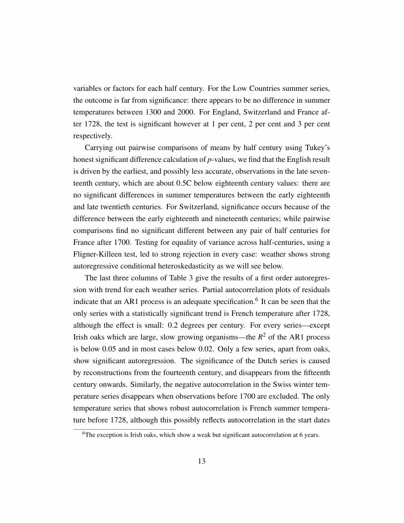
Figure 2: Impact of weather on wheat yields, 1270–1450

To estimate the impact of weather on yields we run a regression of log yieldratios on weather, allowing intercepts and slopes to vary across manors.

logyit = (β0 +β0i)+(β1 +β1i)(st − s̄)+(β2 +β2i)rt + εit

where yit is gross yield per seed on manor i in year t, st − s̄ is the deviation ofestimated summer temperature from its mean value, and rt is tree ring thicknessexpressed in standard deviations from its mean. The intercept and slope havecomponents that vary idiosyncratically across manors β ji ∼ N(0,σ2

β j). It follows

that the intercept is the log yield ratio in a year with average weather, while theslope coefficients are the average percentage changes in yield due to a one degreechange in summer temperature and a one standard deviation change in oak ringthickness. We estimate by restricted maximum likelihood (Pinheiro and Bates,2000, Ch. 2). Plots of the quantiles of the regression residuals against quantiles ofthe normal distribution indicate that this semi-log specificiation appears adequate,apart from some very negative residuals presumably due to episodes of crop dis-ease.

8

Intercept Summer Rings Loglik R̃2 σα N Manors

Wheat 1.2227∗∗ 0.0503∗∗ −0.0565∗∗ −2389 0.2957 0.2042 8439 112(0.0197) (0.0049) (0.004)

Rye 1.286∗∗ 0.0483∗∗ −0.0321∗∗ −597.2 0.1325 0.1372 1134 29(0.0285) (0.0169) (0.0153)

Barley 1.1805∗∗ 0.0035 −0.0087∗∗ −2231.4 0.2481 0.1934 7572 104(0.0195) (0.0052) (0.0043)

Oats 0.8742∗∗ 0.0201 −0.0042 −2648.2 0.1519 0.1417 8290 116(0.0138) (0.0051) (0.0042)

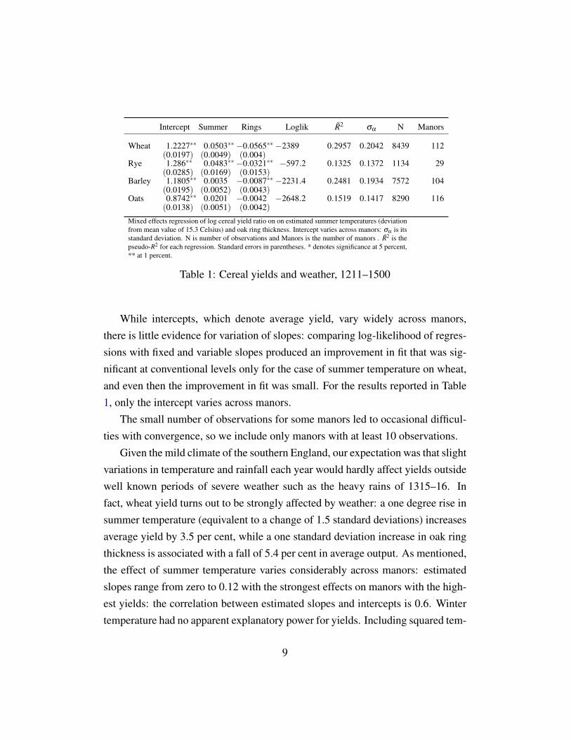
Mixed effects regression of log cereal yield ratio on on estimated summer temperatures (deviationfrom mean value of 15.3 Celsius) and oak ring thickness. Intercept varies across manors: σα is itsstandard deviation. N is number of observations and Manors is the number of manors . R̃2 is thepseudo-R2 for each regression. Standard errors in parentheses. * denotes significance at 5 percent,** at 1 percent.

Table 1: Cereal yields and weather, 1211–1500

While intercepts, which denote average yield, vary widely across manors,there is little evidence for variation of slopes: comparing log-likelihood of regres-sions with fixed and variable slopes produced an improvement in fit that was sig-nificant at conventional levels only for the case of summer temperature on wheat,and even then the improvement in fit was small. For the results reported in Table1, only the intercept varies across manors.

The small number of observations for some manors led to occasional difficul-ties with convergence, so we include only manors with at least 10 observations.

Given the mild climate of the southern England, our expectation was that slightvariations in temperature and rainfall each year would hardly affect yields outsidewell known periods of severe weather such as the heavy rains of 1315–16. Infact, wheat yield turns out to be strongly affected by weather: a one degree rise insummer temperature (equivalent to a change of 1.5 standard deviations) increasesaverage yield by 3.5 per cent, while a one standard deviation increase in oak ringthickness is associated with a fall of 5.4 per cent in average output. As mentioned,the effect of summer temperature varies considerably across manors: estimatedslopes range from zero to 0.12 with the strongest effects on manors with the high-est yields: the correlation between estimated slopes and intercepts is 0.6. Wintertemperature had no apparent explanatory power for yields. Including squared tem-

9

Wheat Rye Barley Oats

Wheat 0.477 0.338 0.237Rye 0.884 0.370 0.305Barley 0.852 0.831 0.599Oats 0.811 0.761 0.876

Table 2: Correlation between annual yields (above diagonal), and nominal prices(below diagonal) of cereals, 1270–1450.

perature and oak rings, to allow for possible non-linear effects of weather, did notproduce large or significant effects.

One thing we know for certain about our weather estimates is that they aremeasured with error, and their coefficient estimates suffer in consequence fromattenuation bias. Using the textbook errors in variable formula, based on theknown relationship of the variables between 1766 and 1900, a regression usingDutch summer temperature and oak ring thickness as proxies for English summertemperature and rainfall respectively will produce coefficients that are 70 per centand 48 per cent respectively of their true values, and to the extent that medievaltemperature estimates are less accurate than these later observations, the underes-timate for temperature will be correspondingly larger.

Other crops were less sensitive to weather, in the order that we would expect.Rye has similar coefficients to wheat, while the spring grains barley and oats showno measurable effect of rainfall, although oats show a slightly positive effect ofsummer temperature.

We see that, in terms of weather risk, spring grains offered the best insuranceto subsistence farmers, and have the added advantages of growing on poorer soilthan wheat, and producing more calories per acre. While we know from medievalaccounts that the staple food of servants, outside harvest time, was dredge, a mix-ture of barley and oats, Kelly and Ó Gráda (2010) show that a better predictorof mortality at all levels of society in the century before the Black Death waswheat yields. This reflects the fact that most families had too little land to support

10

themselves, and worked for wages whose purchasing power reflected wheat yieldswhich determined the prices of other grains. As Table 2 shows, yields of other ce-reals are poorly correlated with wheat, but their prices are strongly correlated.

3 Climate Since the Middle Ages.

To look at how weather deteriorated during the Little Ice Age we analyse severalwidely used annual climate reconstructions up to 2000 for Western Europe, sum-marized in Table 3: Low Countries Summer and Winter temperature from 1301;5

French summer temperature from 1370; Swiss summer and winter temperatureand precipitation from 1525; English summer and winter temperature from 1660,and precipitation from 1766. We also consider two other series that reflect weatherconditions: Irish oaks from 1301 and English wheat yields from 1270.

We start by looking at the stability of each series: can we find structural breakscorresponding to different phases of climate. To do this we apply a Bai and Per-ron (1998) procedure to detect breakpoints in a regression of annual weather on aconstant (including autoregressive terms and a trend did not alter our results ma-terially). We break each series in Table 3 according to the detected break dates.It can be seen that the winter temperature series show a consistent pattern, with abreak occurring in every case around the end of the nineteenth century, with tem-perature rising by 0.6–0.8 C. This common trend appears consistent with globalwarming. Similarly, winters appear to become wetter at this time, in both Englandand Switzerland.

Summer temperatures by contrast show no break in the Low Countries, Swissor English data, while the French data break in 1728 at the time when the modernmercury thermometer is introduced. Swiss summers become noticeably drier after

5Although these series start in AD 800, there are increasing numbers of missing observationsas we go back past 1301 and the authors are less confident of their accuracy, putting them inwider bands that they denote by Roman rather than Arabic numerals. In running times series tests,missing observations during the 14th and early 15th centuries (30 for winter, 11 for summer) wereset at the median value of the entire series. Running tests from the mid-15th century did not changethe reported results materially.

11

Start Mean SD K-W ρ Trend R2

TemperatureNetherlands summer 1301 16.206 0.908 0.358 0.102∗∗ 0.000 0.011Netherlands winter 1301 1.685 1.644 0.305 −0.056 0.000 0.003

1861 2.478 1.714 0.214 0.135 0.005 0.036France summer 1370 0.044 1.03 0.008 0.178∗∗ 0.000 0.032

1728 −0.268 0.76 0.035 −0.083 0.002∗∗ 0.041Switzerland summer 1525 −0.043 0.995 0.040 0.068 0.000 0.007Switzerland winter 1525 −0.426 1.146 0.077 −0.139∗∗ −0.001∗ 0.028

1909 0.126 1.217 0.754 0.086 −0.001 0.008England summer 1660 15.284 0.807 0.012 0.099 0.001 0.015England winter 1660 3.468 1.348 0.013 −0.056 0.002 0.016

1895 4.348 1.287 0.555 0.109 0.007 0.048Precipitation

Switzerland summer 1525 0.216 0.972 0.035 0.120∗ −0.000 0.0221812 −0.072 0.907 0.028 −0.016 0.002 0.009

Switzerland winter 1525 −0.243 0.859 0.251 −0.025 −0.001 0.0081899 0.246 0.997 0.365 0.037 0.005 0.019

England summer 1766 451.132 89.833 0.152 0.087 −0.167 0.0121883 414.459 76.34 0.368 −0.025 0.125 0.004

England winter 1766 450.259 81.516 0.596 0.048 0.024 0.0021864 505.361 90.588 0.349 −0.072 0.256 0.016

OtherIrish oaks 1301 0.000 1.006 0.879 0.332∗∗ 0.000 0.111English wheat 1270 3.586 0.558 0.635 0.117 0.001 0.010

K-W is the p-value of the Kruskal-Wallis rank sum test where data are grouped by half century.Followed by autoregressive coefficient ρ and trend coefficients, and squared correlation R2 forAR(1) regression with time trend. ** denotes a coefficient significant at 1 per cent, estimated withAndrews HAC standard errors. Swiss data end in 1989, Irish oaks in 1993, and English wheat in1450.

Table 3: Summary statistics and tests of autoregression and trend for annualweather indicators until 2000.

the 1810s, and English ones after the 1880s. Among other series, the thickness ofIrish oak growth rings and English medieval yields remain constant.

Next we ask if different half centuries had different temperatures using aKruskall-Wallis procedure to test if different half centuries have higher or lowerranked temperature. Because our data are close to normal, the results in eachcase are the same as the p-value of a regression of annual temperature on dummy

12

variables or factors for each half century. For the Low Countries summer series,the outcome is far from significance: there appears to be no difference in summertemperatures between 1300 and 2000. For England, Switzerland and France af-ter 1728, the test is significant however at 1 per cent, 2 per cent and 3 per centrespectively.

Carrying out pairwise comparisons of means by half century using Tukey’shonest significant difference calculation of p-values, we find that the English resultis driven by the earliest, and possibly less accurate, observations in the late seven-teenth century, which are about 0.5C below eighteenth century values: there areno significant differences in summer temperatures between the early eighteenthand late twentieth centuries. For Switzerland, significance occurs because of thedifference between the early eighteenth and nineteenth centuries; while pairwisecomparisons find no significant different between any pair of half centuries forFrance after 1700. Testing for equality of variance across half-centuries, using aFligner-Killeen test, led to strong rejection in every case: weather shows strongautoregressive conditional heteroskedasticity as we will see below.

The last three columns of Table 3 give the results of a first order autoregres-sion with trend for each weather series. Partial autocorrelation plots of residualsindicate that an AR1 process is an adequate specification.6 It can be seen that theonly series with a statistically significant trend is French temperature after 1728,although the effect is small: 0.2 degrees per century. For every series—exceptIrish oaks which are large, slow growing organisms—the R2 of the AR1 processis below 0.05 and in most cases below 0.02. Only a few series, apart from oaks,show significant autoregression. The significance of the Dutch series is causedby reconstructions from the fourteenth century, and disappears from the fifteenthcentury onwards. Similarly, the negative autocorrelation in the Swiss winter tem-perature series disappears when observations before 1700 are excluded. The onlytemperature series that shows robust autocorrelation is French summer tempera-ture before 1728, although this possibly reflects autocorrelation in the start dates

6The exception is Irish oaks, which show a weak but significant autocorrelation at 6 years.

13

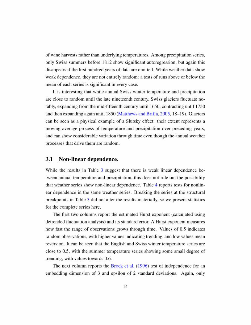
of wine harvests rather than underlying temperatures. Among precipitation series,only Swiss summers before 1812 show significant autoregression, but again thisdisappears if the first hundred years of data are omitted. While weather data showweak dependence, they are not entirely random: a tests of runs above or below themean of each series is significant in every case.

It is interesting that while annual Swiss winter temperature and precipitationare close to random until the late nineteenth century, Swiss glaciers fluctuate no-tably, expanding from the mid-fifteenth century until 1650, contracting until 1750and then expanding again until 1850 (Matthews and Briffa, 2005, 18–19). Glacierscan be seen as a physical example of a Slutsky effect: their extent represents amoving average process of temperature and precipitation over preceding years,and can show considerable variation through time even though the annual weatherprocesses that drive them are random.

3.1 Non-linear dependence.

While the results in Table 3 suggest that there is weak linear dependence be-tween annual temperature and precipitation, this does not rule out the possibilitythat weather series show non-linear dependence. Table 4 reports tests for nonlin-ear dependence in the same weather series. Breaking the series at the structuralbreakpoints in Table 3 did not alter the results materially, so we present statisticsfor the complete series here.

The first two columns report the estimated Hurst exponent (calculated usingdetrended fluctuation analysis) and its standard error. A Hurst exponent measureshow fast the range of observations grows through time. Values of 0.5 indicatesrandom observations, with higher values indicating trending, and low values meanreversion. It can be seen that the English and Swiss winter temperature series areclose to 0.5, with the summer temperature series showing some small degree oftrending, with values towards 0.6.

The next column reports the Brock et al. (1996) test of independence for anembedding dimension of 3 and epsilon of 2 standard deviations. Again, only

14

H σH BDS TLG GARCH σG

TemperatureNetherlands summer 0.523 0.013 0.286 0.096 0.642 0.003Netherlands winter 0.562 0.015 0.855 0.609 0.785 0.011France summer 0.594 0.019 0.000 0.221 0.174 0.003Switzeland summer 0.624 0.022 0.227 0.434 0.888 0.003Switzerland winter 0.51 0.012 0.046 0.697 0.959 0.007England summer 0.579 0.016 0.523 0.883 0.819 0.004England winter 0.472 0.023 0.509 0.503 0.804 0.003

PrecipitationSwitzerland summer 0.637 0.022 0.256 0.071 0.934 0.192Switzerland winter 0.57 0.013 0.777 0.003 0.803 0.003England summer 0.48 0.03 0.466 0.446 0.766 0.013England winter 0.634 0.03 0.24 0.766 0.865 0.006

OtherEnglish wheat 0.545 0.027 0.269 0.274 0.799 0.002Irish oaks 0.393 0.037 0.000 0.551 0.999 0.000

H and σH are the estimated Hurst exponent and its standard error; BDS is the p-value of a BDStest with embedding dimension of 3 with an epsilon value of 2 standard deviations; TLG is thep-value of a Terasvirta-Lin-Granger test for non-linearity in means; GARCH is the coefficient onlagged variance in an AR1 model with GARCH(1,1) errors, and σG is its standard error.

Table 4: Tests for non-linear dependence in annual weather series.

French summer and Irish oaks show significant deviations from independence.Next the Teraesvirta, Lin and Granger (1993) test for non-linearity in means isreported and, in this case, only the Swiss winter rain series shows significant de-partures from linearity.

While the levels of most temperature and rainfall series show little autoregres-sion, their variances do. Specifically we assumed that each series followed an AR1process: yt = β0 +β1yt−1 +εt where the variance σ2

t of εt follows a GARCH(1,1)process σ2

t = α0 +α1ε2t−1 +α2σ2

t−1 estimated assuming a skewed generalized er-ror distribution. In all cases we found that the state coefficient α1 was close tozero, and the final two columns of Table 4 report the coefficient and standard er-ror of the variance coefficient α2. It can be seen that, with the exception again

15

of the unusual French summer estimates, all series shows strong autoregressiveheteroskedasticity.

Applying a Markov switching model to the data in each case indicated fairlyrapid transitions between two regimes with equal means but high and low vari-ances; again consistent with GARCH. Like financial return series, annual weathershows weak dependence in levels, but strong autoregression in variance.

4 Weather in Cities

In the previous Section we saw that a variety of long-run weather constructionsfor Europe indicate that annual weather shows little dependence from year to year,and that summer temperatures during the twentieth century differ little from thosein earlier centuries during the supposed Little Ice Age.

A natural objection to these findings is that these long run weather reconstruc-tions rely at times on strong assumptions, that vitiate any conclusions drawn fromthem. It is therefore worthwhile to see if later, more systematic weather seriesbehave similarly. We therefore examine summer and winter temperatures for Eu-ropean cities in the CDIAC “Updated Global Grid Point Surface Air TemperatureAnomaly Data Set: 1851-1990,” selecting all cities where continuous records goback to 1799 or earlier.

Table 5 looks at temporal dependence in winter temperature. Again, series arebroken where a Bai-Perron procedure indicates structural breaks in levels. Justlike the long-run winter reconstructions in Table 3, the winter temperature seriestend to break in the late nineteenth or early twentieth centuries, with a highertemperature after the break, consistent with global warming. Again, a first orderautoregression with trend finds little evidence of a significant trend or autoregres-sion in the data.

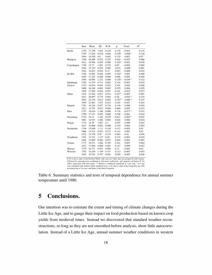
Table 6 repeats the exercise for summer temperature. In this case however,the data appear a considerably noisier with breaks occurring in one city but not innearby neighbours, and falls occurring as well as rises. It would appear that most

16

Start Mean SD K-W ρ Trend R2

Berlin 1757 0.198 2.11 0.025 0.067 0.002 0.011Budapest 1781 −0.28 1.824 0.291 −0.077 −0.007 0.021

1897 0.696 1.708 0.253 0.088 0.005 0.013Copenhagen 1799 −0.317 1.733 0.12 0.047 0.005 0.01

1898 0.847 1.585 0.684 0.089 0.004 0.012De Bilt 1707 1.852 1.837 0.397 −0.119 −0.002 0.016

1859 2.607 1.658 0.604 0.1 −0.001 0.01Edinburgh 1765 2.907 1.212 0.49 −0.168 0.003 0.03

1832 3.749 1.093 0.246 −0.073 0.004 0.025Geneva 1754 0.278 1.447 0.982 −0.058 0.002 0.007

1910 1.366 1.33 0.362 0.082 0.005 0.012Milan 1764 2.198 1.363 0.454 −0.028 −0.004 0.013

1896 2.82 1.165 0.02 0.069 −0.014∗∗ 0.106Munich 1782 −1.193 1.882 0.784 0.025 0.000 0.001Paris 1758 3.142 1.565 0.467 −0.122 −0.003 0.022

1910 3.897 1.522 0.501 0.08 −0.004 0.01Petersburg 1753 −7.128 2.669 0.489 −0.04 0.006∗ 0.019Prague 1775 −2.219 2.165 0.074 0.086 0.005 0.028Stockholm 1757 −3.413 2.19 0.862 −0.023 0.007 0.0139

1882 −2.186 1.994 0.431 0.088 0.000 0.008Trondheim 1762 −2.915 1.8 0.595 −0.18∗∗ 0.006 0.047

1904 −1.274 1.61 0.236 0.222 0.008 0.0521940 −2.698 2.001 0.443 0.165 −0.008 0.03

Vienna 1776 −0.643 1.913 0.581 −0.052 −0.007 0.0161897 0.21 1.784 0.55 0.158 0.001 0.025

Warsaw 1780 −3.608 2.433 0.409 0.042 0.008 0.0111873 −2.219 2.067 0.202 0.083 0.002∗∗ 0.008

Wroclaw 1793 −1.117 2.316 0.018 0.128 0.006 0.045

K-W is the p-value of the Kruskal-Wallis rank sum test where data are grouped by half century.Followed by autoregressive coefficient ρ and trend coefficients, and squared correlation R2 forAR(1) regression with time trend. ** denotes a coefficient significant at 1 per cent, * at 5 per cent,estimated with Andrews HAC standard errors.

Table 5: Summary statistics and tests of temporal dependence for annual wintertemperature until 1980.

structural breaks in these data reflect changes in recording methodology. Again,however, the data for the most part do not exhibit significant autoregression ortrends.

17

Start Mean SD K-W ρ Trend R2

Berlin 1756 17.798 1.045 0.225 0.178 −0.019 0.1161799 17.026 0.918 0.004 0.199∗ 0.008∗∗ 0.1281894 16.939 0.9 0.002 0.135 0.007 0.07

Budapest 1780 20.888 0.932 0.235 0.016 −0.025 0.0681812 19.994 0.859 0.000 0.185∗ −0.001 0.038

Copenhagen 1798 15.77 1.091 0.355 0.05 −0.002 0.0041836 15.253 0.924 0.005 0.074 0.008∗ 0.0811942 16.023 0.816 0.15 0.053 −0.008 0.016

De Bilt 1706 15.681 0.826 0.095 0.262∗∗ 0.001 0.0681849 17.245 0.828 0.004 0.046 −0.005 0.0261940 16.095 1.231 0.000 0.278∗∗ −0.039∗∗ 0.323

Edinburgh 1764 13.579 0.713 0.005 0.129 −0.001 0.019Geneva 1753 16.874 0.641 0.055 0.101 0.005 0.028

1808 16.369 0.881 0.065 0.079 0.004 0.0291928 17.058 0.816 0.057 −0.101 −0.015∗ 0.072

Milan 1763 21.943 0.871 0.074 0.227∗ −0.007 0.0911831 20.897 0.775 0.092 −0.26 0.042∗∗ 0.2341863 22.318 0.812 0.002 0.307∗∗ 0.008∗∗ 0.1971949 21.081 1.031 0.012 0.245 −0.027 0.203

Munich 1781 16.224 0.837 0.754 0.138 0.000 0.0161812 15.707 0.832 0.004 0.069 0.002 0.015

Paris 1757 18.634 1.186 0.000 0.176 −0.071∗∗ 0.5431790 17.121 0.925 0.000 0.106 −0.001 0.016

Petersburg 1752 16.14 1.102 0.078 −0.011 −0.007∗∗ 0.0521881 14.937 1.026 0.002 0.026 0.006 0.034

Prague 1774 16.78 1.067 0.3 0.207 0.000 0.0431837 16.004 0.882 0.000 0.159 0.002 0.045

Stockholm 1756 15.098 1.111 0.194 0.112 −0.003 0.021860 14.331 0.922 0.273 −0.141 0.001 0.021932 15.378 0.87 0.139 0.083 −0.01 0.036

Trondheim 1761 12.721 1.127 0.69 0.132 −0.001 0.0181862 12.069 0.984 0.057 0.042 −0.001 0.003

Vienna 1775 18.551 1.046 0.765 0.241 0.007 0.0641812 17.696 0.808 0.001 0.147 0.000 0.022

Warsaw 1779 16.771 0.951 0.003 0.12 −0.001 0.02Wroclaw 1792 16.259 1.199 0.157 0.213 −0.007 0.053

1834 16.763 0.787 0.001 0.029 −0.003 0.028

K-W is the p-value of the Kruskal-Wallis rank sum test where data are grouped by half century.Followed by autoregressive coefficient ρ and trend coefficients, and squared correlation R2 forAR(1) regression with time trend. ** denotes a coefficient significant at 1 per cent, * at 5 percent, estimated with Andrews HAC standard errors. L-B is the p-value of the Ljung-Box test withmaximum lag of 10 years, and Hurst is the Hurst Exponent.

Table 6: Summary statistics and tests of temporal dependence for annual summertemperature until 1980.

5 Conclusions.

Our intention was to estimate the extent and timing of climate changes during theLittle Ice Age, and to gauge their impact on food production based on known cropyields from medieval times. Instead we discovered that standard weather recon-structions, so long as they are not smoothed before analysis, show little autocorre-lation. Instead of a Little Ice Age, annual summer weather conditions in western

18

Europe between 1300 and 2000 are weakly dependent draws from a distributionwith a fixed mean but autocorrelated variance; while winter weather behaves sim-ilarly until around 1900, but then warms notably.

Climate therefore appears to have played little role in reducing the harvests onwhich pre-industrial Europeans relied for survival. Our finding is a reminder thatsome of the changes claimed by Lamb (1995) to be consequences of the LittleIce Age have other possible causes. The freezing of the Thames—which for mostpeople is the most salient fact about the Little Ice Age—was due to Old LondonBridge which effectively acted as a dam, creating a large pool of still water whichfroze 12 times between 1660 and 1815. Tidal stretches of the river have not frozensince the bridge was replaced in 1831, even during 1963 which is the third coldestwinter (after 1684 and 1740) in the Central England temperature series that startsin 1660.

Among Dutch artists, Avercamp made a living from his formulaic winterscenes, but such snowscapes rarely feature in the work of his better known con-temporaries, such as Albert Cuyp, Jan van Goyen, or Salomon van Ruisdael. Itbears noting that Breugel’s iconic ‘Hunters in the Snow’ was one of a series of sixpaintings describing different seasons of the year and that none of the others hintsat a Little Ice Age.

For Greenland’s Vikings, competition for resources with the indigenous Inuit,the decline of Norwegian trade in the face of an increasingly powerful GermanHanseatic League, the greater availability of African ivory as a cheaper substi-tute for walrus ivory, overgrazing, plague, and marauding pirates probably allplayed some role in its demise (Brown, 2000); and even if weather did worsen,the more fundamental question remains of why Greenland society failed to adapt(McGovern, 1981). The disappearance of England’s few vineyards is associatedwith increasing wine imports after Bordeaux passed to the English crown in 1152,suggesting that comparative advantage may have played a larger role than climate.

Similarly, the decline of wheat and rye cultivation in Norway from the thir-teenth century may owe more to lower German cereal prices than temperature

19

change (Miskimin, 1975, 59). With worsening climate we would expect wheatyields to fall relative to barley oats (see Table 1) whereas Apostolides et al. (2008,Tables 1A, 1B) find that between the early fifteenth and late seventeenth century,wheat yields show no trend relative to oats, and rise steadily relative to barley.

Finally, demography supports our reservations about a European Little IceAge. We would expect northern Europe to have shown weak population growthas the Little Ice Age forced back the margin of cultivation. In fact, while thepopulation of Europe in 1820 was roughly 2.4 times what it had been in 1500, inNorway the population was about 3.2 times as large, in Switzerland 3.5 times, inFinland 3.9 times, and in Sweden 4.7 times as large as in 1500 (Maddison, 2009).

Appendix: Data Sources and Estimation

• Monthly mean Central England temperature from 1659 are from http://hadobs.-metoffice.com/hadcet/cetml1659on.dat, and the monthly England and Walesprecipitation series from 1766 are from http://hadobs.metoffice.com/hadukp/-data/monthly/HadEWP_monthly_qc.txt.

• The Low Countries temperature series of van Engelen, Buisman and IJnsen(2001) are available at www.knmi.nl/kd/metadata/nederland_wi_zo.html.

• Spring-Summer temperatures in Burgundy, expressed as the deviation fromthe 1960–1989 average from Chuine et al. (2004) are available at http://-www.ncdc.noaa.gov/paleo/pubs/chuine2004/chuine2004.html

• Swiss summer and winter temperature and precipitation from Pfister (1992)are available at ftp://ftp.ncdc.noaa.gov/pub/data/paleo/historical/switzerland/clinddef.txt

• Irish oak ring widths, measured as standard deviations from their mean, areannual deviations from a 30 year moving average. Provided by ProfessorMichael Baillie, Palaeoecology Centre, The Queen’s University of Belfast.

20

• European cities summer and winter temperatures are averages of June toAugust, and December to January temperatures from the jonesnh.dat filein “An Updated Global Grid Point Surface Air Temperature Anomaly DataSet: 1851-1990” available at http://cdiac.ornl.gov/ftp/ndp020/.

• Crop yield data are from Campbell (2007): http://www.cropyields.ac.uk.

• Price data are taken from Robert Allen’s database of Prices and Wagesin London and Southern England, 1259–1914 (http://www.nuff.ox.ac.uk/-users/allen/studer/london.xls).

• Estimation was carried out in R. Panel regressions were estimated usingthe lme4 module, BDS and Teraesvirta tests from tseries module, GARCHfrom fGarch module, and the Hurst exponent from the fARMA module.

References

Apostolides, Alexander, Stephen Broadberry, Bruce Campbell, Mark Overton andBas van Leeuwen. 2008. English Gross Domestic Product, 1300–1700: SomePreliminary Estimates. Working paper University of Warwick. 20

Bai, Jushan and Pierre Perron. 1998. “Estimating and Testing Linear Models WithMultiple Structural Changes.” Econometrica 66:47–78. 11

Brock, W.A., W.D. Dechert, B. LeBaron and J.A. Scheinkman. 1996. “A Testfor Independence Based on the Correlation Dimension.” Econometric Reviews

15:197–235. 14

Brown, Dale M. 2000. “The Fate of Greenland’s Vikings.” Archaeology . Avail-able online: http://www.archaeology.org/online/features/greenland. 19

Burroughs, William James. 2003. Weather Cycles: Real or Imaginary? Seconded. Cambridge: Cambridge University Press. 5

21

Cameron, Rondo E. 1993. A Concise Economic History of the World. Oxford:Oxford University Press. 7

Campbell, Bruce M. S. 2007. Three Centuries of English Crops Yields, 1211–

1491. WWW Document. URL http://www.cropyields.ac.uk. 2, 7, 21

Campbell, Bruce M.S. 2009. “Nature as Historical Protagonist.” Economic His-

tory Review . 6

Chuine, Isabelle, Isabelle Yiou, Nicolas Viovy, Bernard Seguin, Valerie Daux andEmmanuel Le Roy Ladurie. 2004. “Grape ripening as a past climate indicator.”Nature 432(289–290). 20

de Vries, Jan. 1981. Measuring the Impact of Climate on History: The Search forAppropriate Methodologies. In Climate and History, ed. Robert I. Rotberg andTheodore K. Rabb. Princeton: Princeton University Press. 6, 7

Kelly, Morgan and Cormac Ó Gráda. 2010. Living Standards and Mortality sincethe Middle Ages. Working paper School of Economics, University CollegeDublin. 3, 7, 10

Koepke, Nikola and Joerg Baten. 2005. “The Biological Standard of Living inEurope during the Last Two Millennia.” European Review of Economic History

9(01):61–95. 6

Komlos, John. 2003. “An Anthropometric History of Early Modern France.” Eu-

ropean Review of Economic History 70:159–189. 7

Lamb, H. H. 1995. Climate, History and the Modern World. Second ed. London:Routledge. 6, 19

Le Roy Ladurie, Emmanuel. 1971. Times of Feast, Times of Famine: A History of

Climate since the Year 1000. New York: Doubleday. 7

Maddison, Angus. 2009. Statistics on World Population, GDP and Per Capita

GDP, 1-2006 AD. WWW document URL: http://www.ggdc.net/maddison/. 20

22

Mann, Michael E. 2002. Little Ice Age. In Encyclopedia of Global Environmental

Change, ed. Michael C. McCracken and John S. Perry. Wiley. 2, 6

Mann, Michael E., Zhihua Zhang, Scott Rutherford, Raymond S. Bradley, Mal-colm K. Hughes, Drew Shindell, Caspar Ammann, Greg Faluvegi and FenbiaoNi. 2009. “Global Signatures and Dynamical Origins of the Little Ice Age andMedieval Climate Anomaly.” Science 326:1256–1260. 2, 6

Matthews, John A. and Keith R. Briffa. 2005. “The ’Little Ice Age’: Re-evaluationof an evolving concept.” Geografiska Annaler 87 A:17–36. 2, 6, 14

McGovern, T. H. 1981. The Economics of Extinction in Norse Greenland. InClimate and History, ed. T. M. L. Wrigley, M. J. Ingram and G. Farmer. Cam-bridge: Cambridge University Press pp. 404–433. 19

Miskimin, Harry A. 1975. The Economy of Early Renaissance Europe, 1300-

1460. Cambridge: Cambridge University Press. 20

Parker, Geoffrey. 2001. Europe in Crisis: 1598-1648. Oxford: Blackwell. 7

Pfister, C. 1992. Monthly Temperature and Precipitation in Central Europe 1525-1979. In Climate Since A.D. 1500, ed. R.S. Bradley and P.D Jones. London:Routledge. 20

Pinheiro, Jose C. and Douglas M. Bates. 2000. Mixed Effects Models in S and

S-PLUS. New York: Springer. 8

Postan, M. M. 1975. Medieval Economy and Society. Harmondsworth: Penguin.7

Sargent, Thomas J. 1979. Macroeconomics. New York: Academic Press. 5

Slutsky, Eugen E. 1937. “The Summation of Random Causes as the Source ofCyclic Processes.” Econometrica 5:105–146. 5

23

Steckel, Richard. 2004. “New Light on the "Dark Ages": The Remarkably TallStature of Northern European Men during the Medieval Era.” Social Science

History 28:211–229. 6, 7

Tainter, Jospeh A. 1988. The Collapse of Complex Societies. Cambridge: Cam-bridge University Press. 6

Teraesvirta, T, C. F. Lin and C. W. J. Granger. 1993. “Power of the Neural NetworkLinearity Test.” Journal of Time Series Analysis 14:209–220. 15

van Engelen, A.F.V., J. Buisman and F. IJnsen. 2001. A Millennium of Weather,Winds and Water in the Low Countries. In History and Climate: Memories of

the Future?, ed. P. D. Jones, A. E. J. Ogilvie, T. D. Davies and K. R. Briffa.Boston: Kluwer Academic. 20

24