STA218 Introduction to Estimation - University of Torontonosedal/sta218/sta218-chap10.pdf · STA218...

STA218Introduction to Estimation

Al Nosedal.University of Toronto.

Fall 2017

October 26, 2017

Al Nosedal. University of Toronto. Fall 2017 STA218 Introduction to Estimation

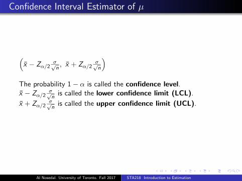
Confidence Interval Estimator of µ

(x̄ − Zα/2

σ√n, x̄ + Zα/2

σ√n

)The probability 1− α is called the confidence level.x̄ − Zα/2

σ√n

is called the lower confidence limit (LCL).

x̄ + Zα/2σ√n

is called the upper confidence limit (UCL).


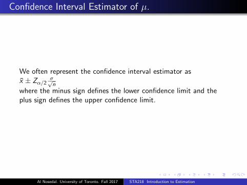
Confidence Interval Estimator of µ.

We often represent the confidence interval estimator asx̄ ± Zα/2

σ√n

where the minus sign defines the lower confidence limit and theplus sign defines the upper confidence limit.


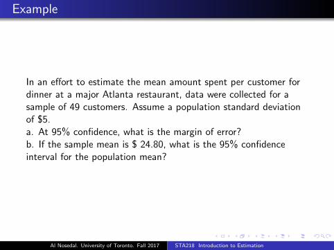
Example

In an effort to estimate the mean amount spent per customer fordinner at a major Atlanta restaurant, data were collected for asample of 49 customers. Assume a population standard deviationof $5.a. At 95% confidence, what is the margin of error?b. If the sample mean is $ 24.80, what is the 95% confidenceinterval for the population mean?


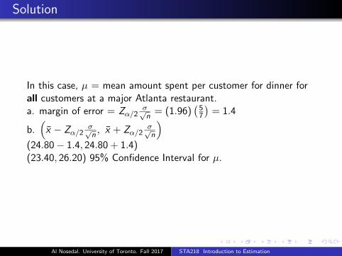
Solution

In this case, µ = mean amount spent per customer for dinner forall customers at a major Atlanta restaurant.a. margin of error = Zα/2

σ√n

= (1.96)(57

)= 1.4

b.(x̄ − Zα/2

σ√n, x̄ + Zα/2

σ√n

)(24.80− 1.4, 24.80 + 1.4)(23.40, 26.20) 95% Confidence Interval for µ.


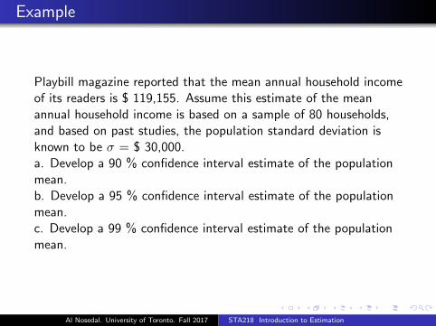
Example

Playbill magazine reported that the mean annual household incomeof its readers is $ 119,155. Assume this estimate of the meanannual household income is based on a sample of 80 households,and based on past studies, the population standard deviation isknown to be σ = $ 30,000.a. Develop a 90 % confidence interval estimate of the populationmean.b. Develop a 95 % confidence interval estimate of the populationmean.c. Develop a 99 % confidence interval estimate of the populationmean.


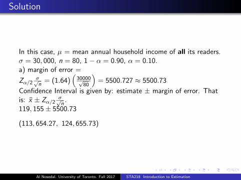
Solution

In this case, µ = mean annual household income of all its readers.σ = 30, 000, n = 80, 1− α = 0.90, α = 0.10.a) margin of error =

Zα/2σ√n

= (1.64)(30000√

80

)= 5500.727 ≈ 5500.73

Confidence Interval is given by: estimate ± margin of error. Thatis: x̄ ± Zα/2

σ√n

.119, 155± 5500.73

(113, 654.27, 124, 655.73)


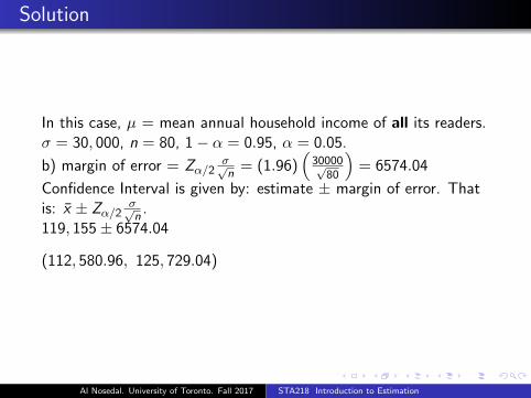
Solution

In this case, µ = mean annual household income of all its readers.σ = 30, 000, n = 80, 1− α = 0.95, α = 0.05.

b) margin of error = Zα/2σ√n

= (1.96)(30000√

80

)= 6574.04


σ√n

.119, 155± 6574.04

(112, 580.96, 125, 729.04)


Solution

In this case, µ = mean annual household income of all its readers.σ = 30, 000, n = 80, 1− α = 0.99, α = 0.01.c) margin of error =

Zα/2σ√n

= (2.57)(30000√

80

)= 8620.042 ≈ 8620.04


σ√n

.119, 155± 8620.04

(110, 534.96, 127, 775.04)


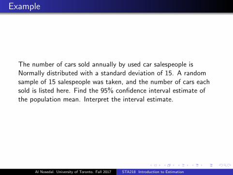
Example

The number of cars sold annually by used car salespeople isNormally distributed with a standard deviation of 15. A randomsample of 15 salespeople was taken, and the number of cars eachsold is listed here. Find the 95% confidence interval estimate ofthe population mean. Interpret the interval estimate.


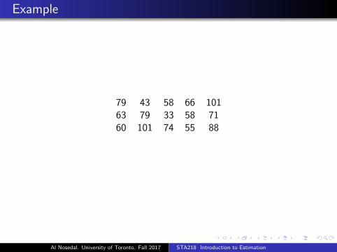
Example

79 43 58 66 10163 79 33 58 7160 101 74 55 88


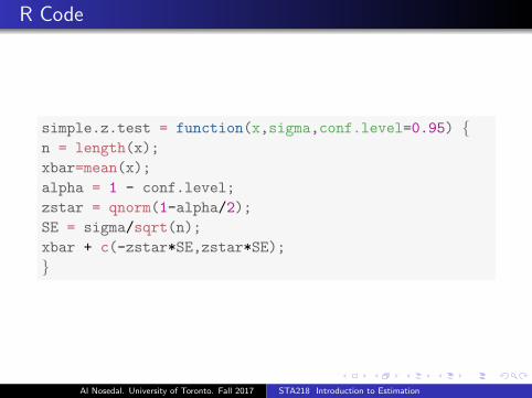
R Code

simple.z.test = function(x,sigma,conf.level=0.95) {n = length(x);

xbar=mean(x);

alpha = 1 - conf.level;

zstar = qnorm(1-alpha/2);

SE = sigma/sqrt(n);

xbar + c(-zstar*SE,zstar*SE);

}


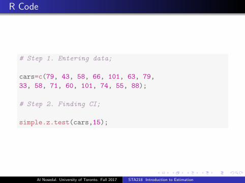
R Code

# Step 1. Entering data;

cars=c(79, 43, 58, 66, 101, 63, 79,

33, 58, 71, 60, 101, 74, 55, 88);

# Step 2. Finding CI;

simple.z.test(cars,15);


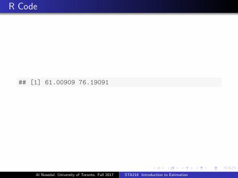
R Code

## [1] 61.00909 76.19091


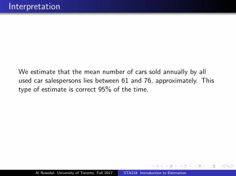
Interpretation

We estimate that the mean number of cars sold annually by allused car salespersons lies between 61 and 76, approximately. Thistype of estimate is correct 95% of the time.


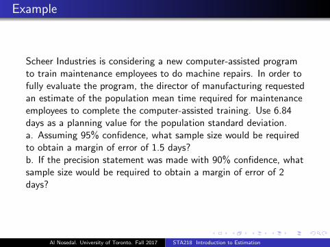
Example

Scheer Industries is considering a new computer-assisted programto train maintenance employees to do machine repairs. In order tofully evaluate the program, the director of manufacturing requestedan estimate of the population mean time required for maintenanceemployees to complete the computer-assisted training. Use 6.84days as a planning value for the population standard deviation.a. Assuming 95% confidence, what sample size would be requiredto obtain a margin of error of 1.5 days?b. If the precision statement was made with 90% confidence, whatsample size would be required to obtain a margin of error of 2days?


Sample size to estimate a mean

n =

(Zα

2σ

B

)2

.

B stands for the bound on the error of estimation.


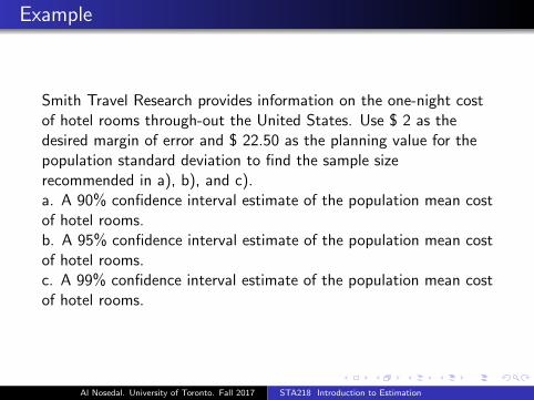
Example

Smith Travel Research provides information on the one-night costof hotel rooms through-out the United States. Use $ 2 as thedesired margin of error and $ 22.50 as the planning value for thepopulation standard deviation to find the sample sizerecommended in a), b), and c).a. A 90% confidence interval estimate of the population mean costof hotel rooms.b. A 95% confidence interval estimate of the population mean costof hotel rooms.c. A 99% confidence interval estimate of the population mean costof hotel rooms.


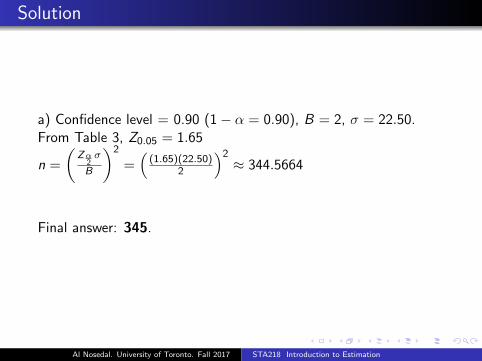
Solution

a) Confidence level = 0.90 (1− α = 0.90), B = 2, σ = 22.50.From Table 3, Z0.05 = 1.65

n =

(Zα

2σ

B

)2

=((1.65)(22.50)

2

)2≈ 344.5664

Final answer: 345.


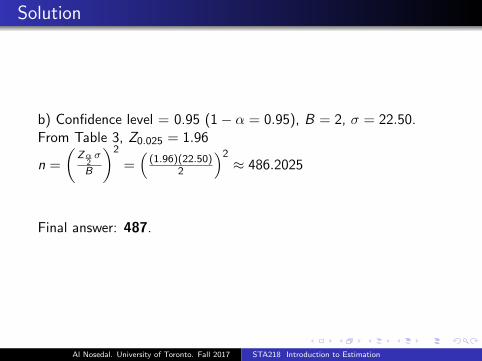
Solution

b) Confidence level = 0.95 (1− α = 0.95), B = 2, σ = 22.50.From Table 3, Z0.025 = 1.96

n =

(Zα

2σ

B

)2

=((1.96)(22.50)

2

)2≈ 486.2025

Final answer: 487.


Solution

c) Confidence level = 0.99 (1− α = 0.99), B = 2, σ = 22.50.From Table 3, Z0.005 = 2.58

n =

(Zα

2σ

B

)2

=((2.58)(22.50)

2

)2≈ 842.4506

Final answer: 843.


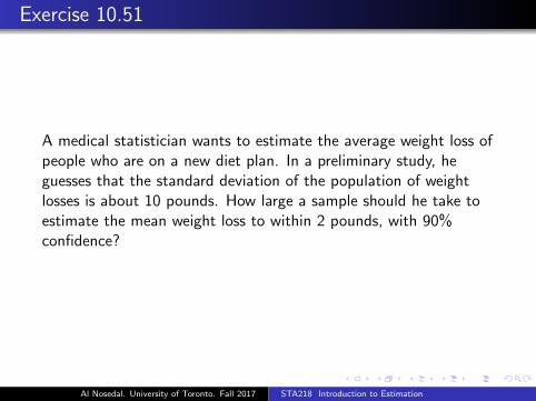
Exercise 10.51

A medical statistician wants to estimate the average weight loss ofpeople who are on a new diet plan. In a preliminary study, heguesses that the standard deviation of the population of weightlosses is about 10 pounds. How large a sample should he take toestimate the mean weight loss to within 2 pounds, with 90%confidence?


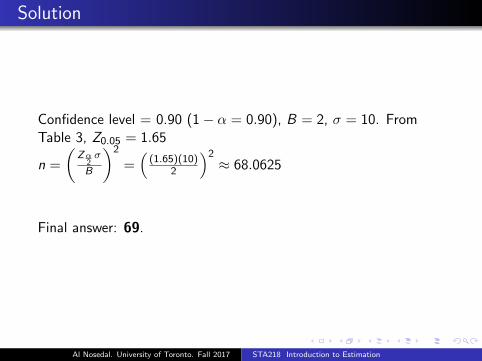
Solution

Confidence level = 0.90 (1− α = 0.90), B = 2, σ = 10. FromTable 3, Z0.05 = 1.65

n =

(Zα

2σ

B

)2

=((1.65)(10)

2

)2≈ 68.0625

Final answer: 69.


STA218 Introduction to Estimation - University of Torontonosedal/sta218/sta218-chap10.pdf · STA218...

Documents

Transcript of STA218 Introduction to Estimation - University of Torontonosedal/sta218/sta218-chap10.pdf · STA218...