Polynomial and FFT

Topics 1. Problem 2. Representation of polynomials 3. The DFT and FFT 4. Efficient FFT implementations 5. Conclusion

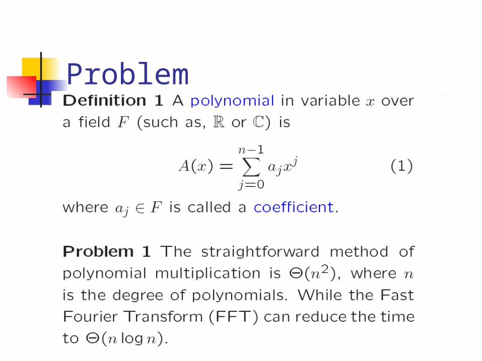
Problem

Representation of Polynomials

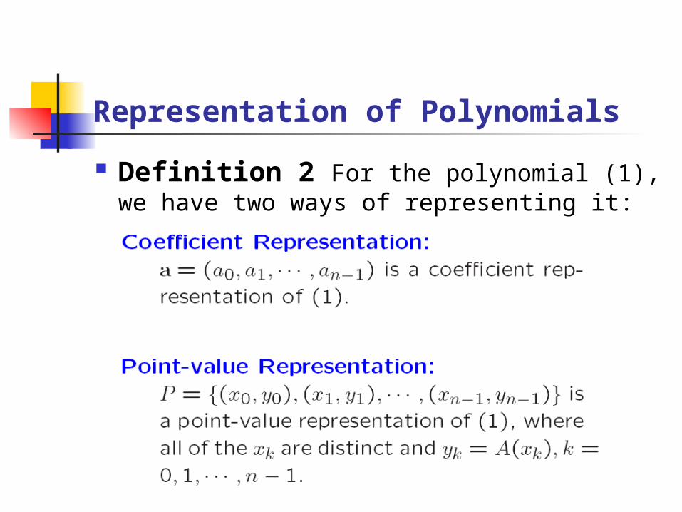
Definition 2 For the polynomial (1), we have two ways of representing it:

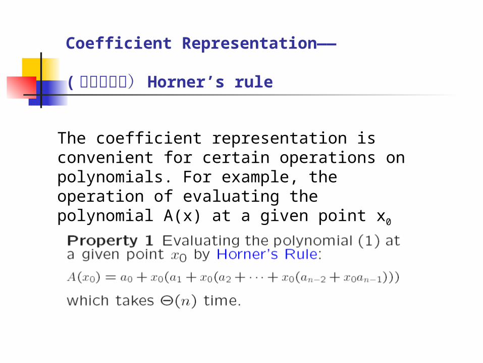
Coefficient Representation—— (秦九韶算法）Horner’s rule

The coefficient representation is convenient for certain operations on polynomials. For example, the operation of evaluating the polynomial A(x) at a given point x0

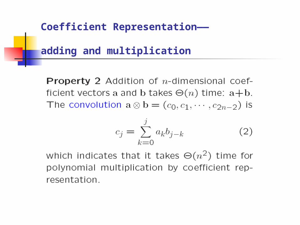
Coefficient Representation—— adding and multiplication

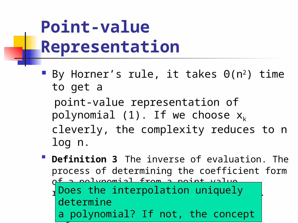
Point-value Representation By Horner’s rule, it takes Θ(n2) time to

get a point-value representation of polynomial

(1). If we choose xk cleverly, the complexity reduces to n log n.

Definition 3 The inverse of evaluation. The process of determining the coefficient form of a polynomial from a point value representation is called interpolation.Does the interpolation uniquely determinea polynomial? If not, the concept ofinterpolation is meaningless.

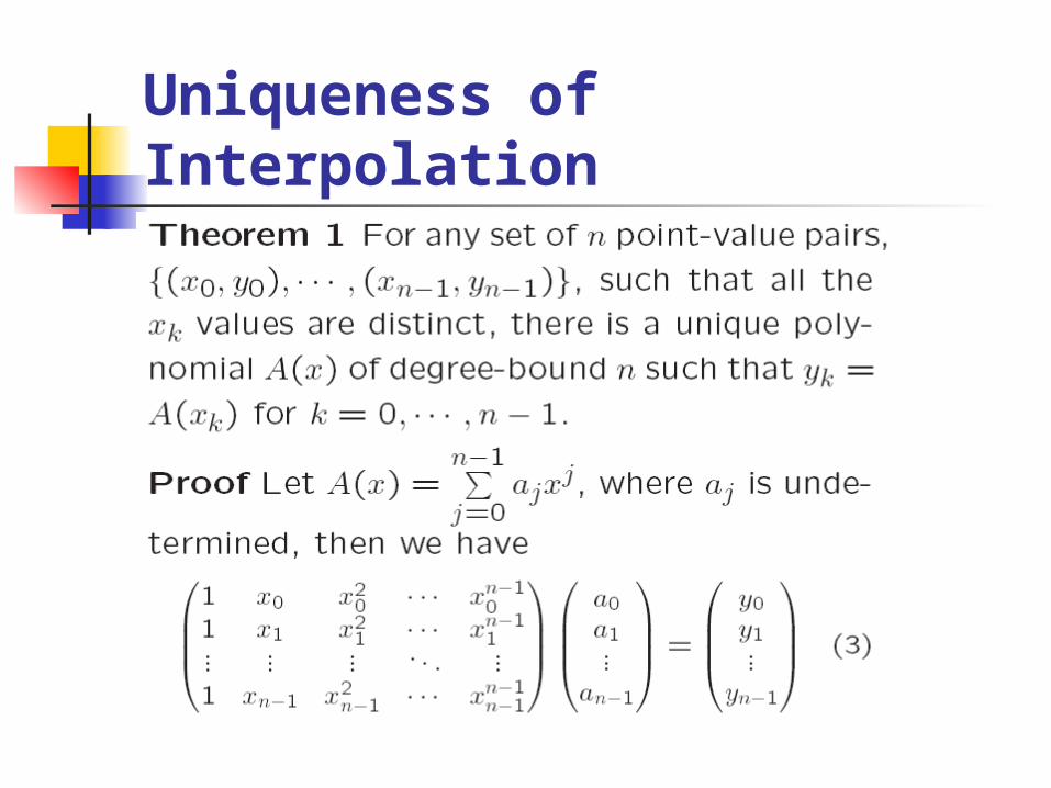
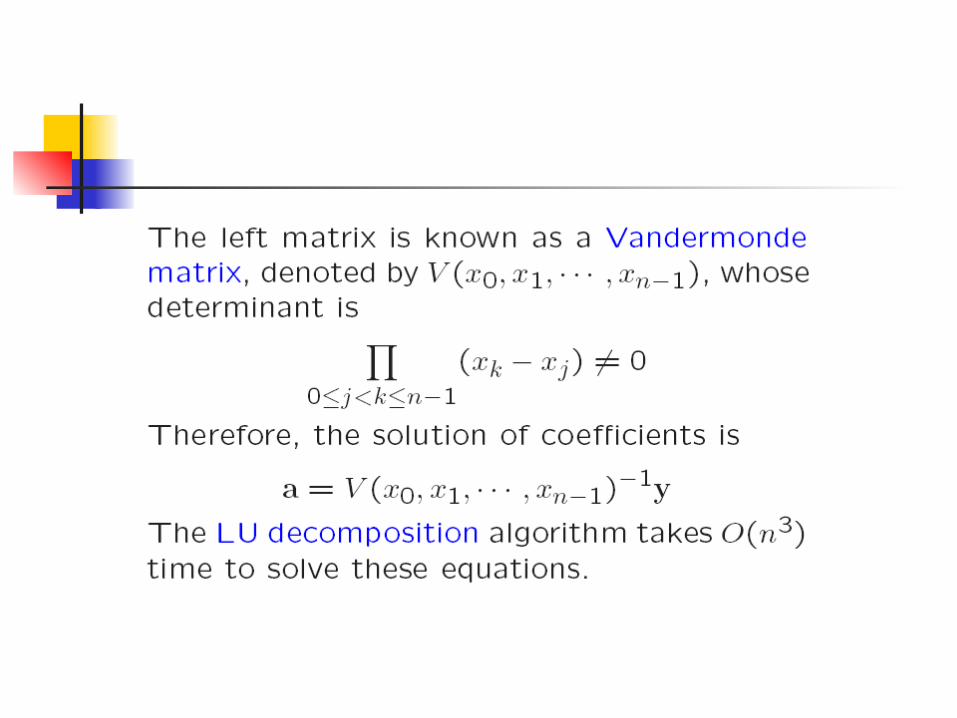
Uniqueness of Interpolation

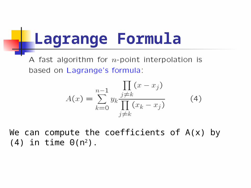
Lagrange Formula

We can compute the coefficients of A(x) by (4) in time Θ(n2).

拉格朗日［ Lagrange, Joseph Louis ， 1736-

1813

● 法国数学家。

● 涉猎力学，著有分析力学。

● 百年以来数学界仍受其理论影响。

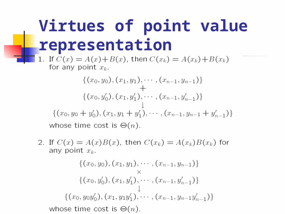
Virtues of point value representation

Fast multiplication of polynomials in coefficient form

Can we use the linear-time multiplication method for polynomials in point-value form to expedite polynomial multiplication in coefficient form?

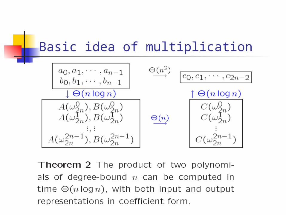
Basic idea of multiplication

Basic idea of multiplication If we choose “complex roots of unity”

as the evaluation points carefully, we can produce a point-value representation by taking the Discrete Fourier Transform of a coefficient vector. The inverse operation interpolation, can be performed by taking the inverse DFT of point value pairs.

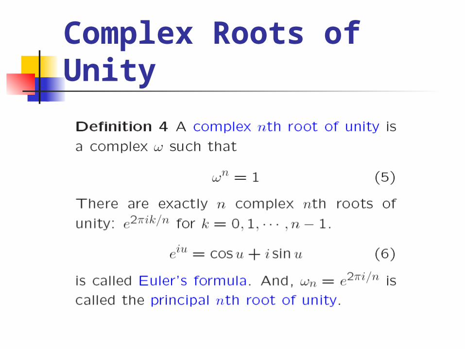
Complex Roots of Unity

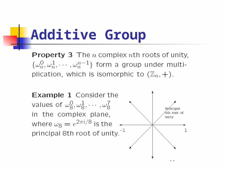
Additive Group

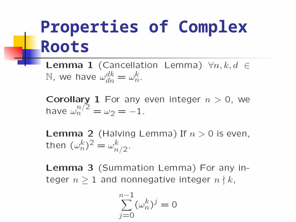
Properties of Complex Roots

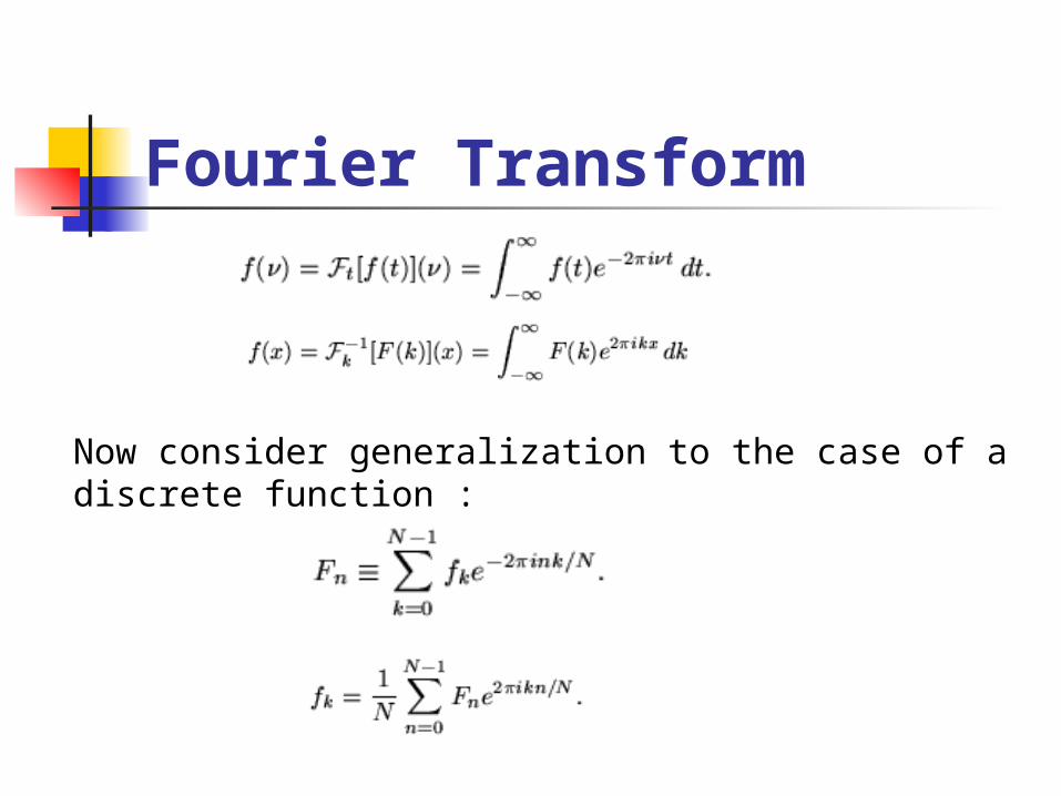
Fourier Transform

Now consider generalization to the case of a discrete function :

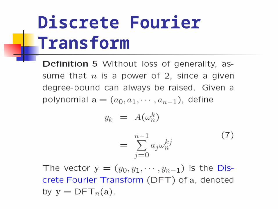
Discrete Fourier Transform

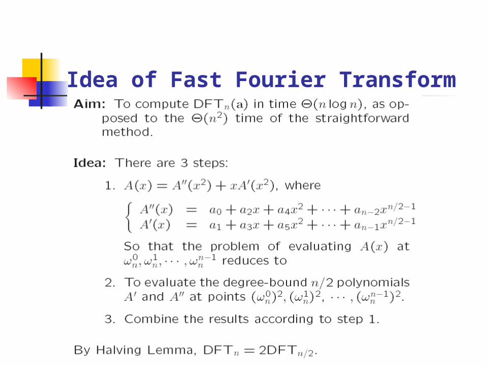
Idea of Fast Fourier Transform

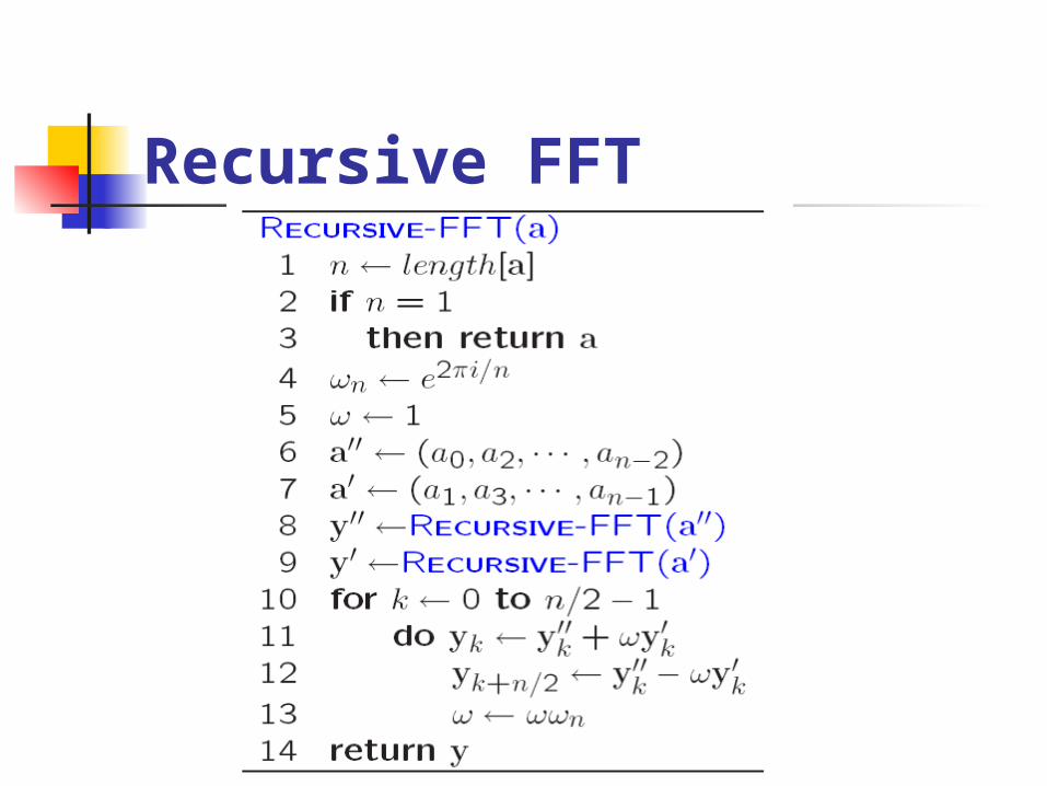
Recursive FFT

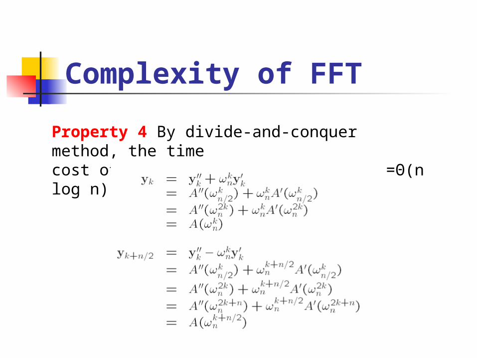
Complexity of FFT

Property 4 By divide-and-conquer method, the timecost of FFT is T(n) = 2T(n/2)+Θ(n) =Θ(n log n).

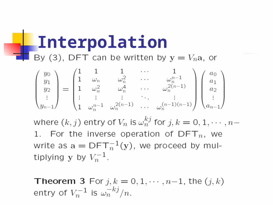
Interpolation

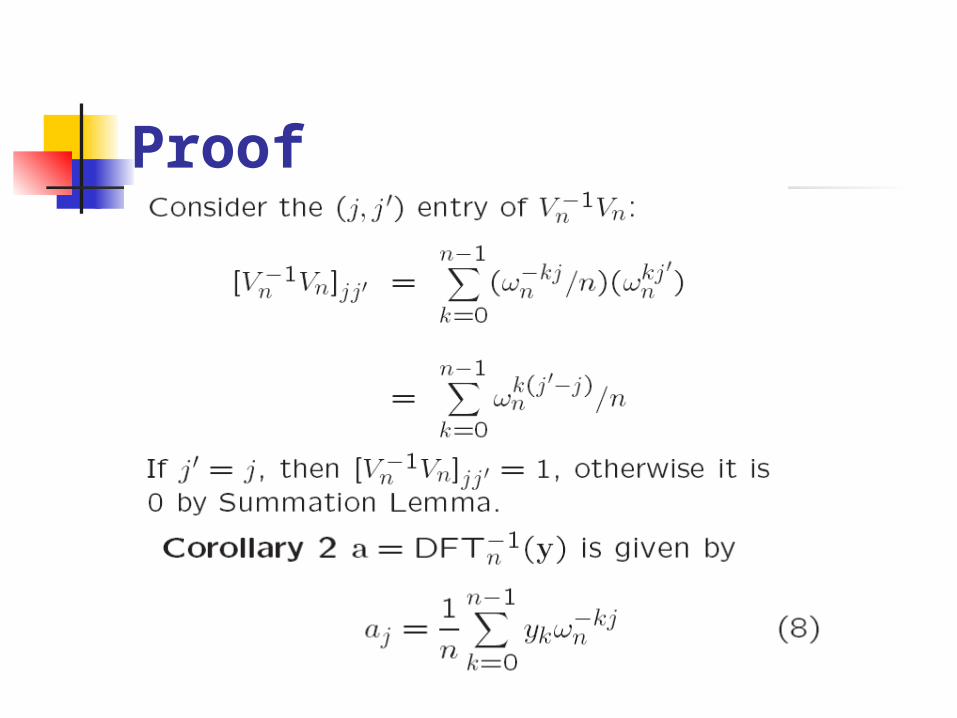
Proof

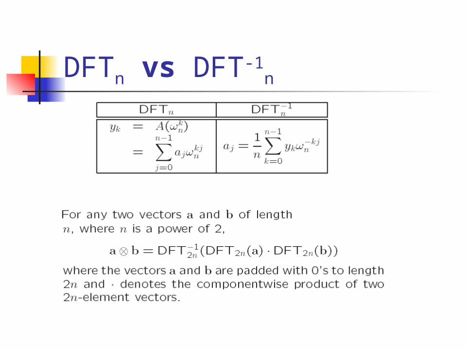
DFTn vs DFT-1n

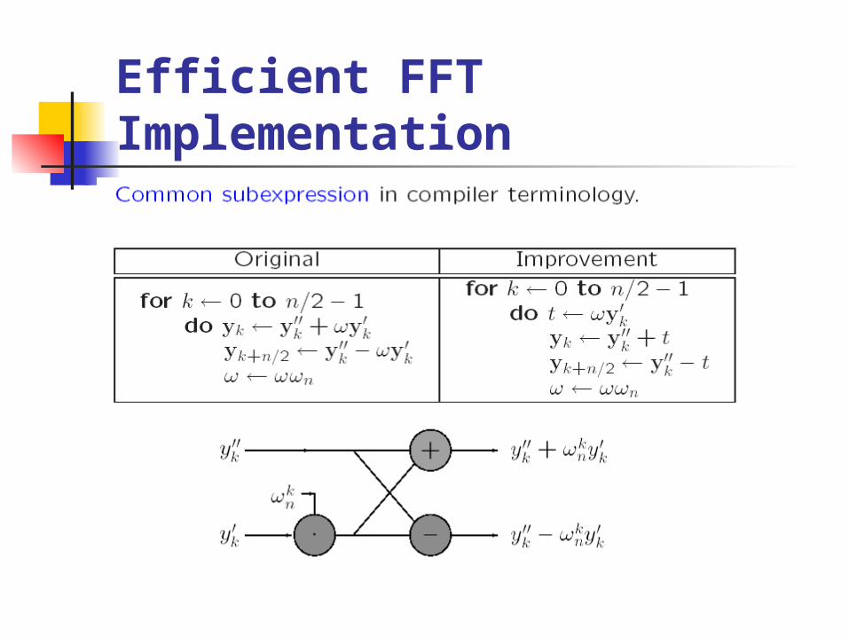
Efficient FFT Implementation

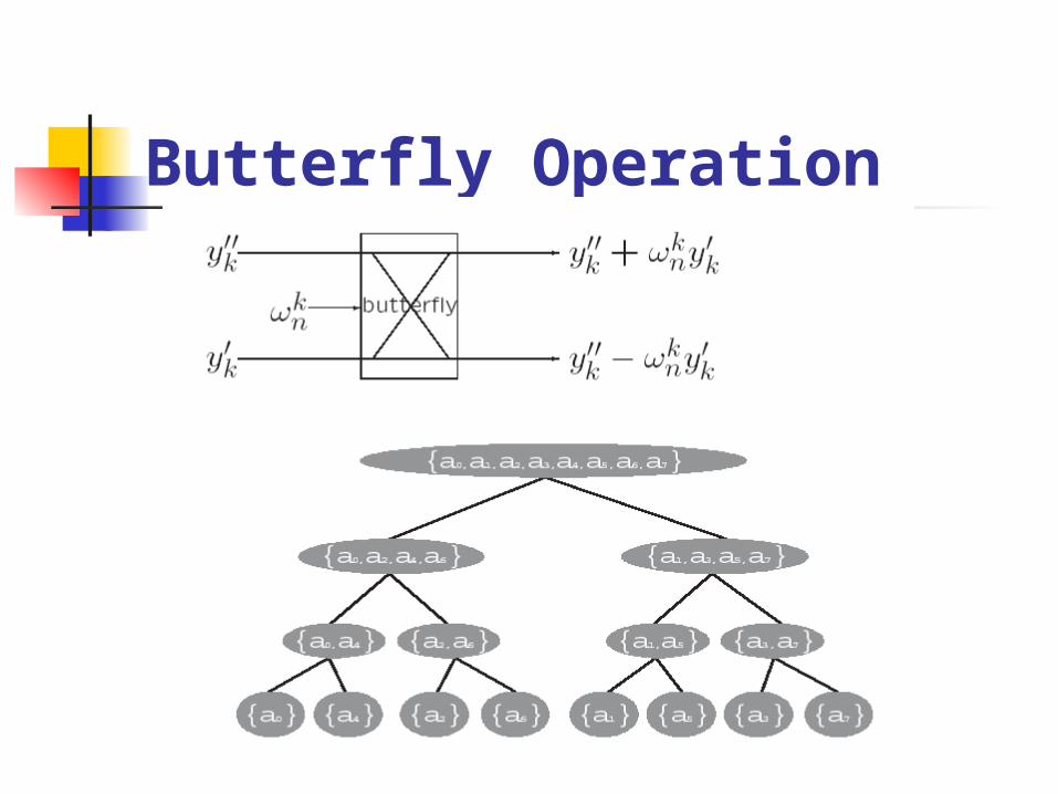
Butterfly Operation

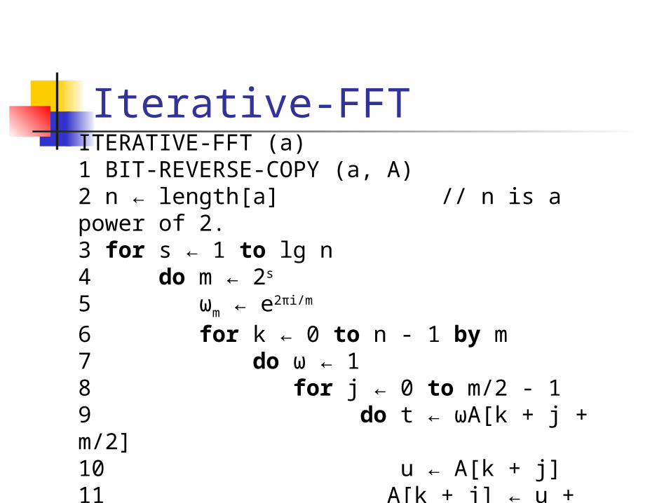
Iterative-FFTITERATIVE-FFT (a)1 BIT-REVERSE-COPY (a, A)2 n ← length[a] // n is a power of 2.3 for s ← 1 to lg n4 do m ← 2s

5 ωm ← e2πi/m

6 for k ← 0 to n - 1 by m7 do ω ← 18 for j ← 0 to m/2 - 19 do t ← ωA[k + j + m/2]10 u ← A[k + j]11 A[k + j] ← u + t12 A[k + j + m/2] ← u - t13 ω ← ω ωm

conclusion

Fourier analysis is not limited to 1-dimensional data. It is widely used in image processing to analyze data in 2 or more dimensions.

Cooley and Tukey are widely credited with devising the FFT in the 1960’s.