學科補習、成績表現與升學結果── 以學測成績與上公立大學為例黃毅志、陳俊瑋 學科補習、成績表現與升學結果──以學測成績與上公立大學為例


科技部TSSCI期刊
期貨與選擇權學刊 Journal of Futures and Options
第九卷第一期 二○一六年四月 Volume 9, Number 1, April 2016

臺灣期貨交易所 2015年4月榮獲「The Asian Banker 2015年度
金融衍生性商品交易所」 2015年9月榮獲「FOW 2015年亞洲區股權類
商品創新契約」 2015年11月榮獲「The Asian Banker 2015年
最佳區域性人民幣期貨交易所」
臺灣期貨交易所繼2004及2009年獲選為Asia Risk雜誌年度風雲
交易所(Derivatives Exchange of the Year)獎項之肯定後,國際財經專
業雜誌亞洲銀行家(The Asian Banker)於2015年4月宣布期交所榮獲
「年度金融衍生性商品交易所」(Financial Derivatives Exchange of the
Year);繼而於9月,因與歐洲期貨交易所跨國合作商品「歐臺期與
歐臺選」(Eurex/TAIFEX Link),榮獲Futures and Options World(FOW)
評選為「2015年亞洲區股權類商品創新契約獎」;11月再獲亞洲銀
行家雜誌肯定,宣布期交所為「2015年最佳區域性人民幣期貨交易
所」(Best Exchange for Offshore RMB FX Futures by Region)。
在主管機關鼎力支持及期貨業界與期交所共同努力下,近年臺
灣期貨市場表現亮眼,2014年交易量首度突破2億口大關,2015年
交易量更成長至2.5億口,為期交所成立以來年度最高量,推動市
場大幅成長原因主要為推出符合交易人多元化需求之商品、交易結
算制度的調整、辦理國內外宣導推廣活動,以及陸續推出多項國際
合作商品所致。
展望未來,期交所將持續以「避險增益、價格發現」為商品及
制度研發之主軸,加快國際合作腳步,達成「活絡期貨交易、服務
實質經濟」目標,並滿足市場參與者各項需求,以不斷強化核心競
爭優勢,為臺灣期貨市場開創新局,注入源源不絕的活力與動能。

期貨與選擇權學刊 Journal of Futures and Options
第九卷 第一期 (中華民國九十七年五月創刊)
發 行 人:劉連煜
總 監:邱文昌
總 編 輯:李存修
編輯委員:王耀輝 古永嘉 朱浩民 李賢源 周行一 俞明德
馬秀如 張森林 張傳章 郭維裕 郭震坤 陳春山
游啟璋 馮震宇 黃金澤 楊光華 葉銀華 廖四郎
薛富井 謝明華
執行編輯:蔡蒔銓
助理編輯:許維敏、矯恒杰、陶富美、蔡季婷
出版者:臺灣期貨交易所股份有限公司
地 址:台北市羅斯福路二段100號14樓 電 話:(02)2369-5678 傳 真:(02)2369-3689 網 址:http://www.taifex.com.tw
編印者:元照出版公司
地 址:台北市館前路18號5樓 電 話:(02)2375-6688 網 址:http://www.angle.com.tw
本刊著作權所有,未經臺灣期貨交易所股份有限公司同意,
不得轉載全部或部分內容。

「期貨與選擇權學刊」 出版政策
臺灣期貨交易所為鼓勵期貨與選擇權領域之學術研究風氣、提
供相關領域學術論文發表管道,以建立與學界之溝通交流平台、吸
引學界關注期貨市場,為臺灣期貨市場之人才培育與制度健全發展
奠定基石,特發行「期貨與選擇權學刊」。
本學刊廣徵有關期貨、選擇權或衍生性商品(含法律規範與制
度)之理論、實證或應用之中、英文學術論文,歡迎海內外學者、
專家及關心期貨市場發展之人士踴躍投稿。
本學刊固定於每年4月、8月及12月出刊,採匿名審稿程序,設
置編輯委員會處理審稿及編輯業務,每篇文稿至少由兩位學者專家
評審,稿件採隨到隨審方式,經刊登之文稿每篇致贈稿酬新台幣1萬元。
本學刊自2013年起榮獲科技部收錄為臺灣社會科學引文索引核
心期刊(TSSCI),並追溯至2010年起算,未來亦將積極申請收錄
於SSCI資料庫,並期望成為期貨與選擇權相關領域之標竿期刊。
欲知更多詳情,請上
期貨與選擇權學刊網站!

編輯手札
本刊發行迄今已逾八個年頭,今年正式邁入第九年,前四年
2008~2011 年的平均每年投稿數僅 13 篇,接下來的四年中
(2012~2015),平均每年投稿數已倍增至26篇,2016年第一季投稿數
7篇,亦能維持高度的投稿能量,而進入TSSCI(2013年)之後,平均
的接受率為32.95%,亦能有效地提昇本刊的質量。
本刊的另一特色是審稿速度極快,2013~2015年的初審平均天數
僅22.18天,2016年第一季更降到僅14.16天。若計算從投稿到審稿定
案的天數,2013~2015年之平均為37.53天,2016年第一季則降為26
天。審稿快速對投稿者相當有利,節省了許多等待的時間,也降低
了投稿的焦慮情緒。2016年底前,本刊將全面採用線上投稿、審
稿,省去了稿件郵寄的時間,相信審稿時間會再進一步縮短。
本期(第九卷第一期)收錄了三篇頗具實務應用價值的文章,包
括王佳真、王尹柔與李君屏探討股價指數之波動性偏態指標與指數
變動之關係;蘇亭丰評估槓桿型與反向型之長短期追蹤績效;以及
洪瑞成與王偉權所分析投機性交易對臺灣期貨市場之影響等,相信
讀者能從中獲得不少啟發。
總編輯 李存修 謹識
於國立臺灣大學
二○一六年四月
Editor’s Notes
At the end of the eighth year since JFO’s inception, we are pleased to
find that the annual number of submissions in the last four years doubled that
in the first four years, 26 vs. 13. The acceptance rate, on the other hand, head-
ed down to 32.95% since TSSCI enlisting in 2013.
Another favorable feature of JFO is high speed of review process. For
the last three years (2013~2015), first review on average took only 22.18
days and shortened to 14.16 days in the first quarter of 2016. If we look at the
length of the full review process until a final decision is made on a submis-
sion, the average in 2013~2015 was 37.53 days and down to 26 days in the
first quarter of 2016. JFO will adopt a new one-line submission and review
system by the end of 2016, hoping to see an even speedier review process.
Three practical papers are included in this first issue of volume nine.
Wang, Wang and Lee document the connections between volatility skew
measures and TAIEX return. Su evaluates the tracking performance of sever-
al newly introduced leveraged and inverse ETF’s. Finally, Hung and Wang
investigate how return and volatility are affected by speculative trading ac-
tivities. I believe that the readers wull gain lots of insights through these arti-
cals.
Editor in Chief
Tsun-siou Lee, Ph.D. At National Taiwan University
April, 2016
期貨與選擇權學刊 第九卷 第一期 2016. 4
目 錄
波動性偏態指標與臺灣
加權股價指數變動率間的關聯 .. 王佳真、王尹柔、李君屏 1
槓桿型與反向型ETF長短期追蹤績效之研究 ........... 蘇亭丰 61
投機交易活動對臺灣期貨市場
報酬與波動的衝擊 ..................................... 洪瑞成、王偉權 103
Journal of Futures and Options
Vol. 9 No. 1 April 2016
CONTENTS
Connections between Volatility Skew Measures and TAIEX Return
Jai-Jen Wang, Yin-Rou Wang, Jin-Ping Lee ................................ 1 An Investigation of Short- and Long-term Tracking Performance of Leveraged and Inverse ETFs
Ting-Feng Su ............................................................................. 61 The Impact of Speculative Trading Activity on Return and Volatility in Taiwan Futures Market
Jui-Cheng Hung, Wei-Chuan Wang ......................................... 103
1
Connections between Volatility Skew Measures and TAIEX Return ‧
波動性偏態指標與臺灣 加權股價指數變動率間的關聯
* Connections between Volatility Skew
Measures and TAIEX Return
王佳真** Jai-Jen Wang
王尹柔*** Yin-Rou Wang
李君屏**** Jin-Ping Lee
* 2015中部財金學術聯盟研討會_期貨與選擇權學刊推薦,完成本刊審稿
程序。 ** 逢甲大學財務金融系。
Department of Finance, Feng-Chia University *** 財團法人中華民國私立學校教職員退休撫卹離職資遣儲金管理委員
會。 The ROC Private School Staff Retirement and Compensation Fund Management Committee
**** 通訊作者︰逢甲大學財務金融系,臺中市西屯區文華路100號。電話:
+886-4-24517250轉4160;傳真:+886-4-24513796;Email: jplee@fcu. edu.tw。 Department of Finance, Feng-Chia University
投稿日期:2015年9月7日;第一次修訂:2015年11月29日;接受刊登日
期:2015年12月9日 Received: Sep. 7, 2015; First Revision: Nov. 29, 2015; Accepted: Dec. 9, 2015

2
Journal of Futures and Options期貨與選擇權學刊 第9卷第1期 201‧ 6年4月
‧
Contents
I. Introduction 1. Motivation 2. Literature Review
II. Methodology 1. Dataset 2. Volatility Skew Measures
2.1 Volatility Skew Measure of Out-of-the-Money Put and At-the-Money Call Options ( OTMPSKEW )
2.2 Volatility Skew Measures of the Realized and Implied Volatilities of Spot Asset and At-the-Money Call Options (RVIV 1 and RVIV 2)
2.3 Volatility Skew Measures of At-the-Money Put and At-the-Money Call Options ( ATMSKEW and
ATMSKEW∆ )
2.4 Volatility Skew Measure of Out-of-the-Money Call and At-the-Money Put Options ( OTMPSKEW )
3. Methodology III. Empirical Results
1. Descriptive Statistics 1.1 Trading Statistics of
Option Contracts 1.2 Descriptive Statistics of
Volatility Skew Measures 2. Empirical Results of
Regression Analyses 2.1 Single Regressions 2.2 Correlations among
Volatility Skew Measures 2.3 Multivariate
Regressions 3. The Effect of Liquidity 4. The Impact of the 2008
Financial Tsunamis IV. Conclusion

3
Connections between Volatility Skew Measures and TAIEX Return ‧
摘 要
本文使用2002年1月至2013年12月的臺灣市場相關數據,透
過歷史波動率與隱含波動率的組合,計算出六種波動性偏態指
標;並觀察不同價性、不同成交量篩選門檻,以及金融風暴期
間、現貨與選擇權市場間的關聯。結果顯示,臺灣證券交易所
加權股價指數的變動率與波動性偏態指標具有和過去文獻一致
的關聯性。亦即當市場偏向牛市氣氛時,由歷史與隱含波動率
算出的賣權波動性偏態指標,會有縮小的統計特徵,而且其後
的現貨市場也會有偏悲觀的趨勢,或是績效變差的轉移特徵。
而當市場偏向熊市氣氛時,買權波動性偏態指標,會有放大的
統計特徵,而且其後的現貨市場也會有偏樂觀的趨勢,或是績
效轉佳的特徵。投資人可以參考本研究結果,納入波動性偏態
指標的資訊來制訂投資決策。
關鍵詞:隱含波動率、歷史波動率、價性、波動性偏態指標、
臺灣證券交易所總加權股價指數(TAIEX) JEL碼:G11, G12.
4
Journal of Futures and Options期貨與選擇權學刊 第9卷第1期 201‧ 6年4月
‧
Abstract
With the considerations of moneyness, liquidity filters, sampling periods, realized and implied volatilities, this paper applies six volatility skew measures to examine the information contents between the spot and option markets in Taiwan from January 2002 to December 2013. We find that these measures significantly correlate with the TAIEX return series, and their relationships are consistent with the expected directions as explained in the literatures. Specifically, when bearish/bullish perception arises, the skew measures of implied volatilities of puts and calls become higher/lower, and the skew measures turn smaller/larger. Moreover, the spot market becomes more pessimistic/optimistic and performs poorly/well. This suggests that investors can exploit the information from volatility skew measures for various investment demands in dealing with their equity positions.
Keywords: Implied Volatility, Realized Volatility, Moneyness, Volatility Skew Measure, Taiwan Stock Exchange Capitalization Weighted Stock Index (TAIEX)
JEL: G11, G12.
5
Connections between Volatility Skew Measures and TAIEX Return ‧
I. Introduction
1. Motivation The Taiwan Futures Exchange (TAIFEX) launched TAIEX
options in 2002. The debut of these options offers more vehicles to meet the alternative needs of investors in Taiwan. The introduction of TAIEX options also provides investors more flexible channels to simultaneously trade instruments in the stock market and the option market for speculative, hedging or arbitrage motives.
The presumptions of frictionless and complete-market in the typical option pricing model, such as the well-known Black-Scholes model, imply that an option contract can be seen as a redundant security. The payoffs from the option contract can be duplicated by an arbitrage portfolio consisting of the underlying asset and a riskless asset. It implies that there is no additional information content that can be extracted from option trading. However, the contradiction of a frictionless assumption and the properties of lower transaction cost, higher leverage, and less restricted short-selling constraint for option trading lead to informed investors tending to trade and release their private information in the option market instead of or prior to their corresponding trading in the spot market. It indicates that option trading provides the function of price discovery in the capital market. A series of studies examine the interaction between the option market and spot market. For example, under the setting of two groups of boundedly rational agents, newswatchers and momentum traders, Hong and Stein (1999) theoretically demonstrate that attempts at
6
Journal of Futures and Options期貨與選擇權學刊 第9卷第1期 201‧ 6年4月
‧
arbitrage may inevitably lead to overreaction over long horizons, and information generated from the option market may lead the stock market in an unstable way due to traders’ different levels of rationality and their different investing styles.
Chakravarty, Guien and Mayhew (2004) address the role of price discovery played by the option market as well. They empirically estimate an option market’s contribution to price discovery to be about 17% on average based on five years of stock and option data for 60 U.S. firms, further finding that the contribution level is affected by trading volume and spreads in both markets. Hong, Torous and Valkanov (2007) investigate whether the returns of industry portfolios are able to predict the movements of stock markets through spot and option positions. Their empirical results of the nine largest equity markets in the world, including the U.S., reveal remarkably similar patterns and suggest that stock markets react with a delay to information not only contained in industry about their fundamentals, but also contained in the option markets. Lien and Shrestha (2009, 2014) generalize an information share measure developed by Hasbrouck (1995) to examine the price discovery process among the interrelated securities markets. They apply the measure to investigate the information content released in the credit default swap (CDS) market and the bond market. The result indicates that the price discovery mostly takes place in the CDS market. Xie and Mo (2014) use the panel data of Chinese stock market to examine the impact of the introduction of CSI 300 index futures on stock market volatility. They find that the spot price experiences a long-term trend of diminishing volatility after the commencing of CSI 300 index futures.
7
Connections between Volatility Skew Measures and TAIEX Return ‧
In the field of the empirical connection between an option and its underlying asset, the literature seems to pay more attention to the leading-lagging relationship between the return or price series of the two markets. Some studies have recently begun to highlight the junction of volatility and return series between the two markets. For example, Banerjee et al. (2007) find that both the levels and innovations in implied volatility have significant predictive power for future returns on the market portfolio. Bali and Hovakimian (2009) test the significance of the information spillover effect between option and stock markets, noting empirical evidence that the volatility spillover effect takes place from the option market to the stock market, which implies that informed traders tend to first take actions in the option market with their private information.
Goyal and Saretto (2009) construct decile portfolios by sorting stocks on the difference between historical realized volatility and at-the-money implied volatility. A zero-cost trading strategy can be formulated by taking a long (short) position in the decile with a large positive (negative) difference. They find that the strategy produces an economically and statistically significant average monthly return. The profitability result is robust to different market conditions, various industry groupings, diverse levels of option liquidity, and cannot be explained by the usual risk factor models.
Xing, Zhang and Zhao (2010) study the shape of the volatility smirk and find significant cross-sectional predictive power from the smirk for future equity returns. Stocks exhibiting the steepest smirks in their traded options underperform stocks with the least pronounced volatility smirks in their options by around 10.9% per year on a risk-
8
Journal of Futures and Options期貨與選擇權學刊 第9卷第1期 201‧ 6年4月
‧
adjusted basis. This predictability persists for at least six months, and firms with the steepest volatility smirks are those experiencing the worst earnings shocks in the following quarter.
Cremers and Weinbraum (2010) observe the influence of deviations from the put-call parity on future stock returns. They use the difference in implied volatility between pairs of call and put options to measure these deviations and find that stocks with relatively expensive calls outperform stocks with relatively expensive puts by at least 45 basis points per week. Baltussen et al. (2012) assert that the option market contains exploitable information for equity investors for an investable universe of liquid large-cap stocks. Strategies based on several option volatility skew measures can predict returns on the underlying stock. These findings unanimously suggest that information diffuses gradually from the option market into the underlying stock market.
While studies on the leading-lagging relationship between the option and spot markets thrive in the literature, most of them focus on the return or price series of the two markets. It seems that less empirical studies target the junction of the volatility skew measures in the option market and the return or price series in the underlying market, in particular for Taiwan markets. This study thus follows Bali and Hovakimian (2009), Goyal and Saretto (2009), Xing, Zhang and Zhao (2010), Cremers and Weinbraum (2010), and Baltussen et al. (2012) and tries to observe effects from the option market to the stock market in Taiwan through different volatility skew measures developed in the literature. Our empirical results may help investors extend their information contents and improve their investing
9
Connections between Volatility Skew Measures and TAIEX Return ‧
performance by exploiting these volatility skew measures.
2. Literature Review The S-shaped value function of the prospect theory developed by
Kahneman and Tversky (1979) demonstrates that traders hold different risk attitudes when coping with different expectation scenarios according to reference points in their mental accounts. They might be risk averse or risk loving while managing their uncertain investing opportunity sets. The call and put contracts in the option market are able to help satisfy their asymmetric investing demands, and it is the asymmetry of risk attitude or demand that results in a smile-shaped relationship between volatility and moneyness. For example, according to the net buying pressure hypothesis proposed by Bollen and Whaley (2004), the volatility smile is directly related to net buying pressure from public order flow dominated by call option demand. If institutional demand tends to be focused in a particular option series, such as out-of-the-money puts, then the volatility function will be downward sloping.
Trading activities in the option market specifically not only reveal the price expectations of participants on the underlying asset, but also unveil their different facets of risk attitude or behavioral tendency. Thus, practical indicators such as return or volatility measures from option positions may help us comprehend the information contents participants hold in an advanced or earlier sense before what the underlying market shows.
As the traditional literature has noted, the price discovery function of derivative markets comes from the favorable frictions that
10
Journal of Futures and Options期貨與選擇權學刊 第9卷第1期 201‧ 6年4月
‧
spot markets do not have. For example, Black (1975) and Duffie (1996) present that lower transaction cost, higher leverage, and less restricted short-selling constraints in derivative markets make informed traders more active in derivative markets. Fleming, Ostdiek and Whaley (1996) argue that the prices of securities and their derivatives must simultaneously reflect new information in perfectly frictionless and rational markets; otherwise, costless arbitrage profits would be possible. Their empirical results show that the S&P500 index futures market leads the S&P500 stock index and that the S&P100 index option market leads the S&P100 stock index.
The no-arbitrage condition seems to be a reasonable basis of linkage between derivative and underlying markets, and it is an usual behavior assumption in the literature of asset pricing models. However, Hong and Stein (1999) demonstrate that owing to different information-processing capabilities and different investing styles of traders, the linkage between derivative and underlying markets may not be perfect and simultaneous. Thus, the no-arbitrage pricing equilibrium might be dampened by the rationality friction of an over- or under-reaction.
Buraschi and Jackwerth (2001) do not take the viewpoint that an option is a redundant position, because additional priced risk factors such as stochastic interest rates or jumps result in a time-varying or stochastic diffusion term in the spot return process. Using daily S&P500 index options data from 1986-1995, their empirical findings are inconsistent with deterministic volatility models, but are consistent with stochastic models that incorporate these additional priced risk factors. It is stochasticity that makes the information generated by
11
Connections between Volatility Skew Measures and TAIEX Return ‧
implied volatility measures in the option market more valuable in an earlier-step sense in contrast to the spot market.
Chakravarty, Guien and Mayhew (2004) find evidence of significant price discovery in the option market. While the results suggest that both leverage and liquidity play important roles in promoting price discovery, the option market tends to be more informative on average when option trading volume is high, when stock volume is low, when option effective spreads are narrow, and when stock spreads are wide. They also investigate whether the estimates of price discovery in the option market differ across options of different strike prices. On average, the information share tends to be slightly higher for out-of-the-money options than at-the-money options, but this result varies cross-sectionally as a function of trading volume and spreads.
Chan and Shih (2005) investigate empirical relationships among time series of futures, spot, and option positions in the Taiwan markets. They find that these series are significantly interrelated to each other in irregular directions. While derivative positions, including both futures and option positions, significantly lead their spot counterparts, the leading-lagging relationship between the futures and option series is not monotonic. Hong, Torous and Valkanov (2007) develop the hypothesis that the gradual diffusion of information across markets leads to cross-asset return predictability. They test the cross-predictability relationship among industry portfolios and market indices using data from stock markets around the world, finding remarkably similar patterns supporting the gradual-information-diffusion hypothesis among the nine largest stock markets. They assert
12
Journal of Futures and Options期貨與選擇權學刊 第9卷第1期 201‧ 6年4月
‧
that the pervasive empirical results suggest much more work remains to be done, in particular looking at stocks and the options listed on them. Moreover, the gradual information diffusion effect or the price discovery function can be detected or proxied by volatility measures in the spot and option markets.
Traditional volatility measures, such as the historical volatility in the underlying market, represent the realized uncertain degree of the past spot price or return series, while the implied volatility in the option market can proxy the current expectations that traders hold for the future spot price or return series. For example, Frijns, Tallau and Tourani-Rad (2010) develop an implied volatility index for the Australian stock market and assess the information content of the index. They find that the index contains more information than the traditional volatility measures and significantly improves the forecasting power for the future stock market.
Xing, Zhang and Zhao (2010) suggest the combination of realized and implied volatilities with the considerations of different features of option contracts can be more informative. They develop an out-of-the-money volatility skew measure by the difference between the implied volatilities estimated by the out-of-the money put options and the at-the-money call options to examine the relationship between the volatility skew and the future stock returns. They assert that the volatility skew contains the information of the possibility of a negative price jump, the expected magnitude of the price jump, and the premium to compensate the investors for bearing price jump risk.
Several studies have proposed similar volatility skew measures combined with other features of option contracts. For example, Bali
13
Connections between Volatility Skew Measures and TAIEX Return ‧
and Hovakimian (2009) find a negative and significant relationship between expected stock returns and their volatility measures, which are the spreads of realized or implied volatility between call and put contracts. They take their measures as proxies for volatility risk and take the correlations of expected stock return and the volatility measures as proxies for jump risk. Their empirical results indicate significant information flows from individual equity options to individual stocks. Goyal and Saretto (2009) find that information contained in their volatility skew measures produces an economically and statistically significant average monthly return, which is robust to different market conditions, to stock risks-characteristics, to various industry groupings, to option liquidity characteristics, and cannot be explained by the typical risk factor models.
Cremers and Weinbraum (2010) use the difference in implied volatility between pairs of call and put options as their volatility skew measure. They find that both levels and changes in the measure matter for future stock returns and suggest that the option market can affect its underlying market for information-based rather than friction-based reasons only. Baltussen et al. (2012) find that their volatility skew measures can be applied to formulate an effective portfolio, which is substantially different from other well-known stock selection strategies. Their portfolio produces an even stronger profitability result with an annualized performance of around 10%, thereby strengthening the relevance of the publicly available information contained in the option market for equity investors.
14
Journal of Futures and Options期貨與選擇權學刊 第9卷第1期 201‧ 6年4月
‧
II. Methodology
1. Dataset Our sample period is from January 2002 to December 2013.
Stock and option data are from Taiwan Economic Journal Data Bank (TEJ), which provides time series data on the spot price, the Taiwan stock exchange capitalization weighted stock index (TAIEX), and the time series associated with the option contracts such as open interest, volume, and number of days to maturity. It also computes realized and implied volatilities for all listed options with different contract specifications.1 To calculate realized and implied volatilities for each trading day, TEJ first computes the standard deviation of daily TAIEX return, S, within the window of its previous 260 trading days. And an annualized percentage version of realized volatility can be produced by the formula, 260 /100S × , which is the base to be utilized for
different contracts. The implied volatilities are estimated with observed market data in the theoretical Black-Scholes formula with the Newton-Rahpson iteration methodology. The threshold to stop iteration is set to be less than 0.5 between observed and theoretical premiums.2
1 There is a series of TAIEX option contracts with different maturity dates in
the market and the options are traded 15 minutes longer than the spot market. It is worthy to note that the empirical results may be masked by the potential nonsynchronous problem. However, due to the cost of data collection, the daily data instead of intraday data is applied for the empirical analysis in this study.
2 For the complete specification and methodology, please refer to the Taiwan
15
Connections between Volatility Skew Measures and TAIEX Return ‧
On the other hand, in order to obtain the most informative dataset, we employ three criteria as filters to refine the empirical results: (1) liquidity, (2) nearness, and (3) moneyness. As Baltussen et al. (2012) note, the liquidity and nearness requirements make option contracts investable for many traders. The sample of option contracts with zero trading volume is also excluded. Because most activity in options is concentrated in the short end, we select nearby options with the remaining maturity of 10-40 trading days, or approximately a calendar length of one month.
The third criterion, moneyness, is another important dimension of option information content. For example, Xing, Zhang and Zhao (2010) claim that an out-of-the-money put is a natural place for informed traders with negative news to place their trades. If there is an overwhelming pessimistic perception of the stock, investors would tend to buy put options either for protection against future stock price drops (hedge purpose) or for a high potential return on the long put positions (speculation purpose). Thus, we follow Xing, Zhang and Zhao (2010) and Baltussen et al. (2012) to categorize option contracts by the moneyness types and calculate various volatility skew measures thereafter.
We specifically use different ratio ranges of the strike price (K) to the stock index (S) to define the moneyness types. For instance, a call option in our empirical study is defined as at-the-money (ATM) when the ratio of K to S (K/S) is between 0.95 and 1.05, and is abbreviated as ATMC. A put option is defined as out-of-the-money (OTM) when
Economic Journal Data Bank and Benninga (1989).
16
Journal of Futures and Options期貨與選擇權學刊 第9卷第1期 201‧ 6年4月
‧
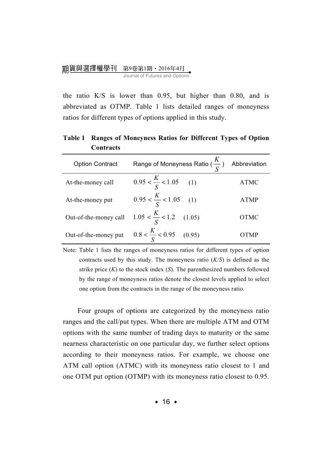
the ratio K/S is lower than 0.95, but higher than 0.80, and is abbreviated as OTMP. Table 1 lists detailed ranges of moneyness ratios for different types of options applied in this study.
Table 1 Ranges of Moneyness Ratios for Different Types of Option
Contracts
Option Contract Range of Moneyness Ratio (KS
) Abbreviation
At-the-money call 05.195.0 <<SK
(1)
ATMC
At-the-money put 05.195.0 <<SK
(1)
ATMP
Out-of-the-money call 1.21.05 <<SK
(1.05)
OTMC
Out-of-the-money put 0.950.8 <<SK
(0.95)
OTMP
Note: Table 1 lists the ranges of moneyness ratios for different types of option contracts used by this study. The moneyness ratio (K/S) is defined as the strike price (K) to the stock index (S). The parenthesized numbers followed by the range of moneyness ratios denote the closest levels applied to select one option from the contracts in the range of the moneyness ratio.
Four groups of options are categorized by the moneyness ratio
ranges and the call/put types. When there are multiple ATM and OTM options with the same number of trading days to maturity or the same nearness characteristic on one particular day, we further select options according to their moneyness ratios. For example, we choose one ATM call option (ATMC) with its moneyness ratio closest to 1 and one OTM put option (OTMP) with its moneyness ratio closest to 0.95.
17
Connections between Volatility Skew Measures and TAIEX Return ‧
These closest levels, applied to deal with contracts of the same nearness characteristic and call/put type, are adopted by Xing, Zhang and Zhao (2010) and Baltussen et al. (2012) and are denoted by the parenthesized numbers followed by the moneyness ratio ranges in Table 1.
2. Volatility Skew Measures Following the methodologies adopted by Bali and Hovakimian
(2009), Goyal and Saretto (2009), Xing, Zhang and Zhao (2010), Cremers and Weinbraum (2010), and Baltussen et al. (2012), we apply liquidity, nearness, and moneyness filters to refine our dataset. We also develop some volatility skew measures here to exert information contents in the Taiwan option and stock markets.
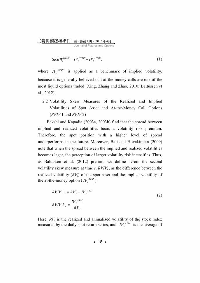
2.1 Volatility Skew Measure of Out-of-the-Money Put and At-the-Money Call Options ( OTMPSKEW )
Gârleanu, Pedersen and Poteshman (2009) and Xing, Zhang and Zhao (2010) assert that a pessimistic informed trader tends to buy a put either for hedge or for speculation purpose. As more and more informed traders come out with a pessimistic perception of the underlying asset, the buying pressure on the out-of-the-money put and its premium will increase, which associates the implied volatility of the put contract with bad news about the future spot price. Thus, the first volatility skew measure at time t, OTMP
tSKEW , is defined as the
difference between the implied volatility of the out-of-the-money put ( OTMP
tIV ) and the implied volatility of the at-the-money call ( ATMC
tIV ):
18
Journal of Futures and Options期貨與選擇權學刊 第9卷第1期 201‧ 6年4月
‧
ATMCt
OTMPt
OTMPt IVIVSKEW −= , (1)
where ATMCtIV is applied as a benchmark of implied volatility,
because it is generally believed that at-the-money calls are one of the most liquid options traded (Xing, Zhang and Zhao, 2010; Baltussen et al., 2012).
2.2 Volatility Skew Measures of the Realized and Implied Volatilities of Spot Asset and At-the-Money Call Options (RVIV 1 and RVIV 2)
Bakshi and Kapadia (2003a, 2003b) find that the spread between implied and realized volatilities bears a volatility risk premium. Therefore, the spot position with a higher level of spread underperforms in the future. Moreover, Bali and Hovakimian (2009) note that when the spread between the implied and realized volatilities becomes lager, the perception of larger volatility risk intensifies. Thus, as Baltussen et al. (2012) present, we define herein the second volatility skew measure at time t, RVIVt , as the difference between the realized volatility (RVt) of the spot asset and the implied volatility of the at-the-money option ( ATM
tIV ):
1
2
ATMt t t
ATMt
tt
RVIV RV IV
IVRVIV
RV
= −
=
(2)
Here, RVt is the realized and annualized volatility of the stock index measured by the daily spot return series, and ATM
tIV is the average of
19
Connections between Volatility Skew Measures and TAIEX Return ‧
the implied volatility of the at-the-money call and the at-the-money put options. Note that RVIV 1 and RVIV 2 are equivalent, but different in scales. Moreover, RVIV 1 is of the original scale while RVIV 2 is of its percentage term and is our third volatility skew measure.
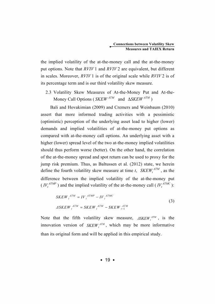
2.3 Volatility Skew Measures of At-the-Money Put and At-the-Money Call Options ( ATMSKEW and ATMSKEW∆ )
Bali and Hovakimian (2009) and Cremers and Weinbaum (2010) assert that more informed trading activities with a pessimistic (optimistic) perception of the underlying asset lead to higher (lower) demands and implied volatilities of at-the-money put options as compared with at-the-money call options. An underlying asset with a higher (lower) spread level of the two at-the-money implied volatilities should thus perform worse (better). On the other hand, the correlation of the at-the-money spread and spot return can be used to proxy for the jump risk premium. Thus, as Baltussen et al. (2012) state, we herein define the fourth volatility skew measure at time t, ATM
tSKEW , as the
difference between the implied volatility of the at-the-money put ( ATMP
tIV ) and the implied volatility of the at-the-money call ( ATMCtIV ):
1
ATM ATMP ATMCt t t
ATM ATM ATMt t t
SKEW IV IV
∆SKEW SKEW SKEW −
= −
= − (3)
Note that the fifth volatility skew measure, ATMt∆SKEW , is the
innovation version of ATMtSKEW , which may be more informative
than its original form and will be applied in this empirical study.
20
Journal of Futures and Options期貨與選擇權學刊 第9卷第1期 201‧ 6年4月
‧
2.4 Volatility Skew Measure of Out-of-the-Money Call and At-the-Money Put Options ( OTMPSKEW )
With more optimistic informed traders active in the option market, the buying pressure on the out-of-the-money call becomes larger and its premium will increase, which associates the implied volatility of the call contract with good news about the future spot price. Here, the sixth volatility skew measure, OTMPSKEW , is defined as the difference between the implied volatility of the out-of-the-money call ( OTMC
tIV ) and the implied volatility of the at-the-money put ( ATMP
tIV ):
OTM C OTM C ATM Pt t tSKEW IV IV= − , (4)
where ATMPtIV is applied as a benchmark of implied volatility in
contrast to the out-of-the-money calls, because at-the-money options are the most liquid positions for traders.
We apply the six volatility skew measures to investigate empirical connections between the option and spot markets in Taiwan. Table 2 summarizes their components, symbolic definitions, and expected directions of correlation with the spot market in the literature.

Table 2 Volatility Skew Measures’ Components, Symbolic Definitions and Expected Directions of Correlation with the Spot Market
Components Symbolic Definition Expected Directions of Correlation with the Spot Market
Implied volatilities of out-of-the-money put and at-the-money call
ATMCt
OTMPt
OTMPt IVIVSKEW −= Negative
ATMttt IVRVRVIV −=1 Positive Realized volatility of the spot
asset and implied volatility of at-the-money call 2
ATMt
tt
IVRVIVRV
= Negative
ATMCt
ATMPt
ATMt IVIVSKEW −= Negative Implied volatilities of at-the-
money put and at-the-money call 1
ATM ATM ATMt t tSKEW SKEW SKEW −∆ = − Negative
Implied volatilities of out-of-the-money call and at-the-money put
ATMPt
OTMCt
OTMCt IVIVSKEW −= Positive
Note: Table 2 summarizes components, symbolic definitions and expected directions of correlation with the spot market in the literature. The symbol IV denotes the implied volatility of option positions, while the symbol RV denotes the realized volatility of the spot position.
21 ‧Connections betw
een Volatility Skew
M
easures and TA
IEX
Return
22
Journal of Futures and Options期貨與選擇權學刊 第9卷第1期 201‧ 6年4月
‧
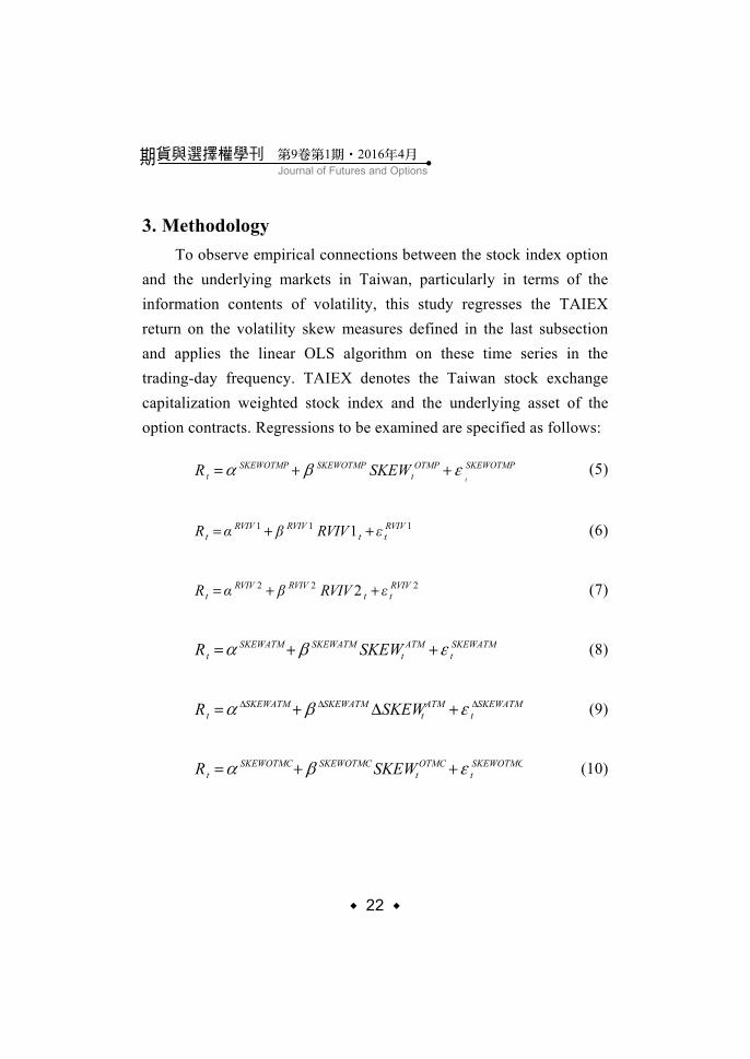
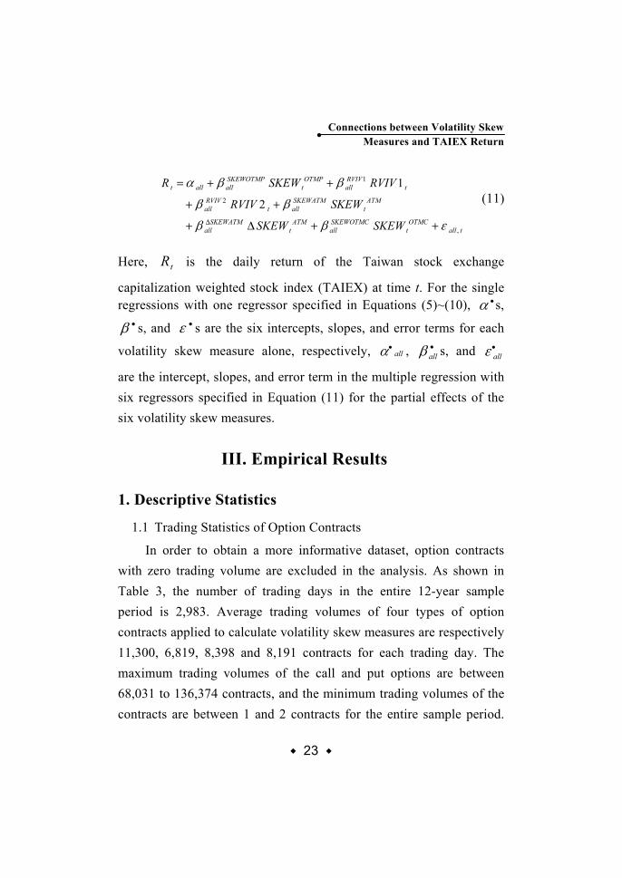
3. Methodology To observe empirical connections between the stock index option
and the underlying markets in Taiwan, particularly in terms of the information contents of volatility, this study regresses the TAIEX return on the volatility skew measures defined in the last subsection and applies the linear OLS algorithm on these time series in the trading-day frequency. TAIEX denotes the Taiwan stock exchange capitalization weighted stock index and the underlying asset of the option contracts. Regressions to be examined are specified as follows:
SKEWOTMPOTMPt
SKEWOTMPSKEWOTMPt t
SKEWR εβα ++= (5)
1 1 11RVIV RVIV RVIVt t tR α β RVIV ε= + + (6)
2 2 22RVIV RVIV RVIVt t tR α β RVIV ε= + + (7)
SKEWATMt
ATMt
SKEWATMSKEWATMt SKEWR εβα ++= (8)
SKEWATMt
ATMt
SKEWATMSKEWATMt SKEWR ∆∆∆ +∆+= εβα (9)
SKEWOTMCt
OTMCt
SKEWOTMCSKEWOTMCt SKEWR εβα ++= (10)
23
Connections between Volatility Skew Measures and TAIEX Return ‧
tallOTMC
tSKEWOTMCall
ATMt
SKEWATMall
ATMt
SKEWATMallt
RVIVall
tRVIVall
OTMPt
SKEWOTMPallallt
SKEWSKEW
SKEWRVIV
RVIVSKEWR
,
2
1
2
1
εββ
ββ
ββα
++∆+
++
++=
∆
(11)
Here, tR is the daily return of the Taiwan stock exchange
capitalization weighted stock index (TAIEX) at time t. For the single regressions with one regressor specified in Equations (5)~(10), •α s,
•β s, and •ε s are the six intercepts, slopes, and error terms for each
volatility skew measure alone, respectively, all•α , •
allβ s, and •allε
are the intercept, slopes, and error term in the multiple regression with six regressors specified in Equation (11) for the partial effects of the six volatility skew measures.
III. Empirical Results
1. Descriptive Statistics
1.1 Trading Statistics of Option Contracts
In order to obtain a more informative dataset, option contracts with zero trading volume are excluded in the analysis. As shown in Table 3, the number of trading days in the entire 12-year sample period is 2,983. Average trading volumes of four types of option contracts applied to calculate volatility skew measures are respectively 11,300, 6,819, 8,398 and 8,191 contracts for each trading day. The maximum trading volumes of the call and put options are between 68,031 to 136,374 contracts, and the minimum trading volumes of the contracts are between 1 and 2 contracts for the entire sample period.
24
Journal of Futures and Options期貨與選擇權學刊 第9卷第1期 201‧ 6年4月
‧
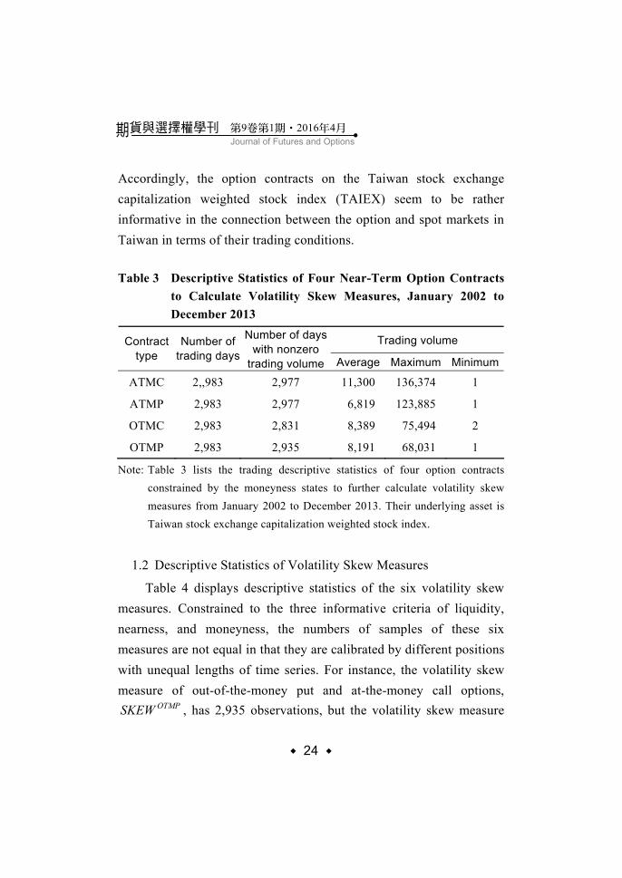
Accordingly, the option contracts on the Taiwan stock exchange capitalization weighted stock index (TAIEX) seem to be rather informative in the connection between the option and spot markets in Taiwan in terms of their trading conditions.
Table 3 Descriptive Statistics of Four Near-Term Option Contracts
to Calculate Volatility Skew Measures, January 2002 to December 2013
Trading volume Contracttype
Number of trading days
Number of days with nonzero
trading volume Average Maximum Minimum
ATMC 2,,983 2,977 11,300 136,374 1
ATMP 2,983 2,977 6,819 123,885 1
OTMC 2,983 2,831 8,389 75,494 2
OTMP 2,983 2,935 8,191 68,031 1
Note: Table 3 lists the trading descriptive statistics of four option contracts constrained by the moneyness states to further calculate volatility skew measures from January 2002 to December 2013. Their underlying asset is Taiwan stock exchange capitalization weighted stock index.
1.2 Descriptive Statistics of Volatility Skew Measures
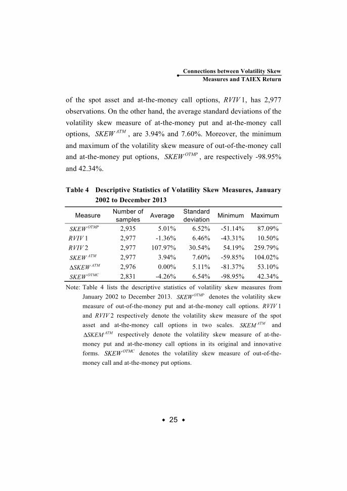
Table 4 displays descriptive statistics of the six volatility skew measures. Constrained to the three informative criteria of liquidity, nearness, and moneyness, the numbers of samples of these six measures are not equal in that they are calibrated by different positions with unequal lengths of time series. For instance, the volatility skew measure of out-of-the-money put and at-the-money call options,
OTMPSKEW , has 2,935 observations, but the volatility skew measure
25
Connections between Volatility Skew Measures and TAIEX Return ‧
of the spot asset and at-the-money call options, RVIV 1, has 2,977 observations. On the other hand, the average standard deviations of the volatility skew measure of at-the-money put and at-the-money call options, ATMSKEW , are 3.94% and 7.60%. Moreover, the minimum and maximum of the volatility skew measure of out-of-the-money call and at-the-money put options, OTMPSKEW , are respectively -98.95% and 42.34%.
Table 4 Descriptive Statistics of Volatility Skew Measures, January
2002 to December 2013
Measure Number of samples Average Standard
deviation Minimum Maximum OTMPSKEW 2,935 5.01% 6.52% -51.14% 87.09%
RVIV 1 2,977 -1.36% 6.46% -43.31% 10.50% RVIV 2 2,977 107.97% 30.54% 54.19% 259.79%
ATMSKEW 2,977 3.94% 7.60% -59.85% 104.02% ATMSKEW∆ 2,976 0.00% 5.11% -81.37% 53.10%
OTMCSKEW 2,831 -4.26% 6.54% -98.95% 42.34% Note: Table 4 lists the descriptive statistics of volatility skew measures from
January 2002 to December 2013. OTMPSKEW denotes the volatility skew measure of out-of-the-money put and at-the-money call options. RVIV 1 and RVIV 2 respectively denote the volatility skew measure of the spot asset and at-the-money call options in two scales. ATMSKEM and
ATMSKEM∆ respectively denote the volatility skew measure of at-the-money put and at-the-money call options in its original and innovative forms. OTMCSKEW denotes the volatility skew measure of out-of-the-money call and at-the-money put options.
26
Journal of Futures and Options期貨與選擇權學刊 第9卷第1期 201‧ 6年4月
‧
2. Empirical Results of Regression Analyses
2.1 Single Regressions
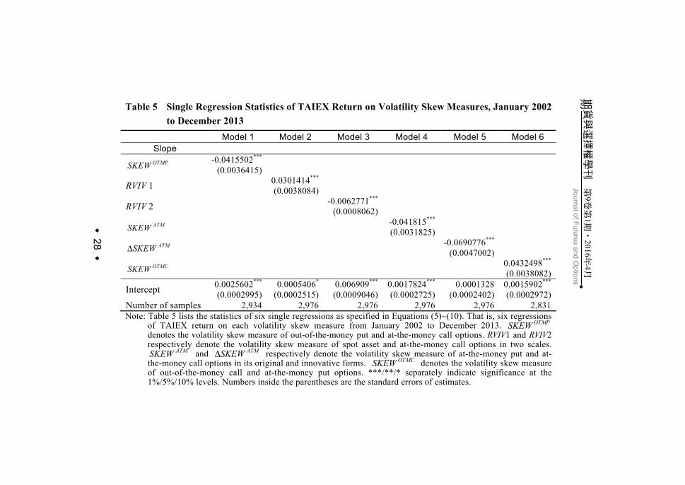
Table 5 lists the statistics of single regressions as specified in Equations (5)~(10). That is, regressions of TAIEX return on each volatility skew measure are conducted separately from January 2002 to December 2013. In terms of the slope estimates in Models 1~6, each volatility skew measure correlates with TAIEX return at the 1% significance level, which means all of the measures are full of information contents about the spot market. In particular, their slope estimates are all consistent with the expected directions of correlation with the spot market in the literature as noted in Table 2.
For instance, OTMPSKEW , the volatility skew measure of out-of-the-money put and at-the-money call options, significantly and negatively correlates with TAIEX return. Its estimated slope is -0.0415502, which is consistent with the reasoning in the literature that as informed pessimistic traders become more active than other ones in option and spot markets, OTMPSKEW will get larger and spot return will get smaller (Gârleanu, Pedersen and Poteshman, 2009; Xing, Zhang and Zhao, 2010).
RVIV 1, the volatility skew measure of the spot asset and at-the-money call options, significantly and positively correlates with TAIEX return This is consistent with the argument in the literature that as the perception of volatility or jump risk in the spot market escalates, the implied volatility or the price of option positions increases faster or to a larger degree than the realized volatility does, and hence RVIV 1 will get smaller and the spot asset tends to underperform in the future. The
27
Connections between Volatility Skew Measures and TAIEX Return ‧
same reasoning applies on RVIV 2 as well, except that the definition of RVIV 2 differs from RVIV 1 at scale and has an inverse +/- direction (Bakshi and Kapadia, 2003a, 2003b; Bali and Hovakimian, 2009). Their estimated slopes are respectively 0.0301414 and -0.0062771.
ATMSKEW , the volatility skew measure of at-the-money put and at-the-money call options, significantly and negatively correlates with TAIEX return. This is consistent with the similar reasoning in the literature as OTMPSKEW , but it is specified in terms of the at-the-money put position rather than the out-of-the-money one. In other words, a larger ATMSKEW or a positive ATMSKEW∆ usually comes when the spot market underperforms (Bali and Hovakimian, 2009; Cremers and Weinbaum, 2010; Baltussen et al., 2012). Their estimated slopes are respectively -0.041815 and -0.0690776.
In contrast to the pessimistic perception that comes with put contracts, OTMPSKEW reveals its information contents through an optimistic perception with the call contracts. As informed optimistic traders become more active than other ones in option and spot markets, implied volatility or the premium of the out-of-the-money call contracts will get higher and the spot return will tend to outperform. As shown in Table 5, OTMPSKEW , the volatility skew measure of out-of-the-money call and at-the-money put options, significantly and positively correlates with TAIEX return, and its estimated slope is 0.0432498.
28
期貨與選擇權學刊
第
9卷
第1期
201‧
6年
4月
Journal of Futures and O
ptions
‧
Table 5 Single Regression Statistics of TAIEX Return on Volatility Skew Measures, January 2002 to December 2013 Model 1 Model 2 Model 3 Model 4 Model 5 Model 6
Slope OTMPSKEW -0.0415502***
(0.0036415)
RVIV 1 0.0301414***
(0.0038084)
RVIV 2 -0.0062771***
(0.0008062)
ATMSKEW -0.041815***
(0.0031825) ATMSKEW∆ -0.0690776***
(0.0047002)OTMCSKEW 0.0432498***
(0.0038082)
Intercept 0.0025602***
(0.0002995)0.0005406*
(0.0002515)0.006909***
(0.0009046)0.0017824***
(0.0002725) 0.0001328
(0.0002402)0.0015902***
(0.0002972)Number of samples 2,934 2,976 2,976 2,976 2,976 2,831Note: Table 5 lists the statistics of six single regressions as specified in Equations (5)~(10). That is, six regressions
of TAIEX return on each volatility skew measure from January 2002 to December 2013. OTMPSKEW denotes the volatility skew measure of out-of-the-money put and at-the-money call options. RVIV1 and RVIV2 respectively denote the volatility skew measure of spot asset and at-the-money call options in two scales.
ATMSKEW and ATMSKEW∆ respectively denote the volatility skew measure of at-the-money put and at-the-money call options in its original and innovative forms. OTMCSKEW denotes the volatility skew measure of out-of-the-money call and at-the-money put options. ***/**/* separately indicate significance at the 1%/5%/10% levels. Numbers inside the parentheses are the standard errors of estimates.

29
Connections between Volatility Skew Measures and TAIEX Return ‧
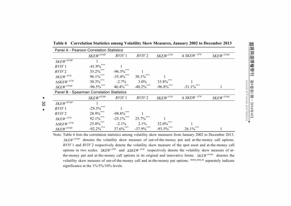
2.2 Correlations among Volatility Skew Measures
This subsection calculates correlations among the six volatility skew measures in order to supplement the analyses of multivariate OLS regressions in the later subsection. There are two types of bivariate correlation coefficients common in the literature. The first one is the Pearson correlation coefficient calculated in terms of variables’ original scales, which can help detect the collinearity problem in econometrics. The second one is the Spearman correlation coefficient calculated in terms of variables’ ranking scales, which is the non-parametric version of the Pearson correlation.
As shown in Panel A and Panel B of Table 6, both Pearson and Spearman statistics display very similar estimated results. Except for ( ATMSKEW∆ , RVIV 1) and ( ATMSKEW∆ , RVIV 2), the correlation coefficients of other pairs are all different from zero at the 1% significance level. In particular, the absolute values of the correlation coefficients of four pairs are extremely high or in excess of 90%. They are ( ATMSKEW , OTMPSKEW ), ( OTMCSKEW , OTMPSKEW ), (RVIV 1, RVIV 2), and ( OTMCSKEW , ATMSKEW ), which means that the collinearity problem cannot be ignored. This problem will be further examined and dealt with in a later subsection of multivariate regression analyses.
30
期貨與選擇權學刊
第
9卷
第1期
201‧
6年
4月
Journal of Futures and O
ptions
‧
Table 6 Correlation Statistics among Volatility Skew Measures, January 2002 to December 2013 Panel A - Pearson Correlation Statistics OTMPSKEW RVIV 1 RVIV 2 ATMSKEW
ATMSKEW∆ OTMCSKEW OTMPSKEW 1
RVIV 1 -41.9%*** 1 RVIV 2 35.2%*** -96.3%*** 1
ATMSKEW 96.1%*** -35.4%*** 30.1%*** 1 ATMSKEW∆ 30.3%*** -2.7% 3.0% 33.8%*** 1
OTMCSKEW -96.5%*** 46.4%*** -40.2%*** -96.8%*** -31.1%*** 1 Panel B - Spearman Correlation Statistics OTMPSKEW RVIV 1 RVIV 2 ATMSKEW
ATMSKEW∆ OTMCSKEW OTMPSKEW 1
RVIV 1 -29.3%*** 1 RVIV 2 28.9%*** -98.8%*** 1
ATMSKEW 92.1%*** -25.1%*** 25.7%*** 1 ATMSKEW∆ 25.0%*** -2.1% 2.1% 32.0%*** 1
OTMCSKEW -92.2%*** 37.6%*** -37.9%*** -93.5%*** 26.1%*** 1 Note: Table 6 lists the correlation statistics among volatility skew measures from January 2002 to December 2013.
OTMPSKEW denotes the volatility skew measure of out-of-the-money put and at-the-money call options. RVIV 1 and RVIV 2 respectively denote the volatility skew measure of the spot asset and at-the-money call options in two scales. ATMSKEW and ATMSKEW∆ respectively denote the volatility skew measure of at-the-money put and at-the-money call options in its original and innovative forms. OTMCSKEW denotes the volatility skew measure of out-of-the-money call and at-the-money put options. ***/**/* separately indicate significance at the 1%/5%/10% levels.
31
Connections between Volatility Skew Measures and TAIEX Return ‧
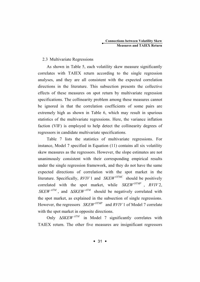
2.3 Multivariate Regressions
As shown in Table 5, each volatility skew measure significantly correlates with TAIEX return according to the single regression analyses, and they are all consistent with the expected correlation directions in the literature. This subsection presents the collective effects of these measures on spot return by multivariate regression specifications. The collinearity problem among these measures cannot be ignored in that the correlation coefficients of some pairs are extremely high as shown in Table 6, which may result in spurious statistics of the multivariate regressions. Here, the variance inflation faction (VIF) is employed to help detect the collinearity degrees of regressors in candidate multivariate specifications.
Table 7 lists the statistics of multivariate regressions. For instance, Model 7 specified in Equation (11) contains all six volatility skew measures as the regressors. However, the slope estimates are not unanimously consistent with their corresponding empirical results under the single regression framework, and they do not have the same expected directions of correlation with the spot market in the literature. Specifically, RVIV 1 and OTMCSKEW should be positively correlated with the spot market, while OTMPSKEW , RVIV 2,
ATMSKEW , and ATMSKEW∆ should be negatively correlated with the spot market, as explained in the subsection of single regressions. However, the regressors OTMPSKEW and RVIV 1 of Model 7 correlate with the spot market in opposite directions.
Only ATMSKEW∆ in Model 7 significantly correlates with TAIEX return. The other five measures are insignificant regressors

32
Journal of Futures and Options期貨與選擇權學刊 第9卷第1期 201‧ 6年4月
‧
under the multivariate regression specification, which contradicts the empirical results of 1% significant slope estimates presented in the subsection of single regressions. We also note that only ATMSKEW∆ is endowed with a small VIF statistic, 1.15. The VIFs of the other five measures are pretty large, ranging from 14.86 to 26.09, which indicate that the collinearity is an issue.
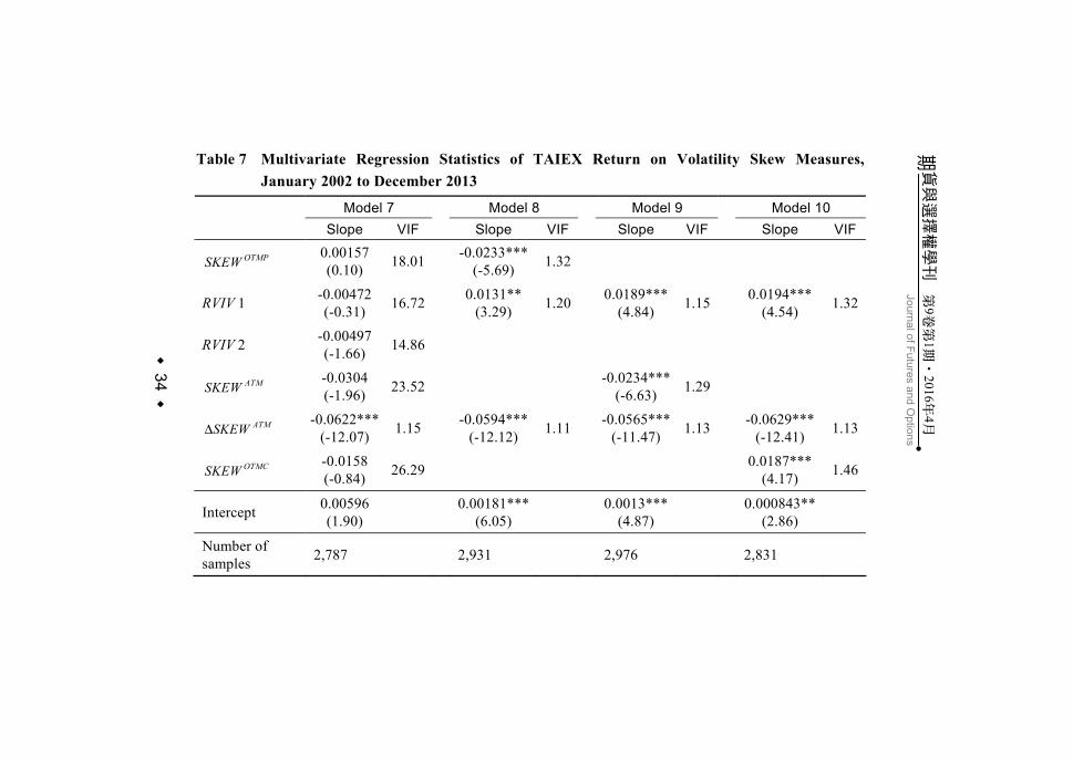
Thus, it is consequently reasonable to discard some regressors of Model 7 to cope with the collinearity problem. ATMSKEW∆ is definitely the first one to be kept in the regression. We then consider the pairs in which the absolute values of correlation coefficients are extremely high or in excess of 90%. They are ( ATMSKEW , OTMPSKEW ), ( OTMCSKEW , OTMPSKEW ), (RVIV 1, RVIV 2), and ( OTMCSKEW , ATMSKEW ). RVIV 1 and RVIV 2 are the same except in different scales. Only one of them should be kept in a regression. It also can be found that two among OTMPSKEW ,
ATMSKEW , and OTMCSKEW can be discarded owing to their high correlations with each other.
Model 8~13 listed in Table 7 demonstrate all possible combinations of regressors after allowing for the above considerations. They are ( OTMPSKEW , RVIV 1, ATMSKEW∆ ), (RVIV 1, ATMSKEW ,
ATMSKEW∆ ), (RVIV 1, ATMSKEW∆ , OTMCSKEW ), ( OTMPSKEW , RVIV 2, ATMSKEW∆ ), (RVIV 2, ATMSKEW , ATMSKEW∆ ), and (RVIV 2, ATMSKEW∆ , OTMCSKEW ), for a total of six multivariate regressions. Note that the VIFs of their regressors range from 1.10 to 1.46, which are pretty small, implying that the collinearity problem may not be an issue for the six multivariate regressions.
In contrast to Model 7, the slope estimates in Models 8~13 are

33
Connections between Volatility Skew Measures and TAIEX Return ‧
overall significant at the 5% or 1% level. In fact, only regressor RVIV 1 in Model 8 is significant at the 5% level, as the other slope estimates in Models 8~13 are significant at the 1% level, which means that all of the measures are full of information contents about the spot market in the collective sense. In particular, the slope estimates are all consistent with the expected directions in the literature as noted in Table 2. The slope estimates are also all consistent with their corresponding empirical results under the single regression framework.
34
期貨與選擇權學刊
第
9卷
第1期
201‧
6年
4月
Journal of Futures and O
ptions
‧
Table 7 Multivariate Regression Statistics of TAIEX Return on Volatility Skew Measures, January 2002 to December 2013
Model 7 Model 8 Model 9 Model 10
Slope VIF Slope VIF Slope VIF Slope VIF
OTMPSKEW 0.00157 (0.10) 18.01 -0.0233***
(-5.69) 1.32
RVIV 1 -0.00472(-0.31) 16.72 0.0131**
(3.29) 1.20 0.0189*** (4.84) 1.15 0.0194***
(4.54) 1.32
RVIV 2 -0.00497(-1.66) 14.86
ATMSKEW -0.0304 (-1.96) 23.52 -0.0234***
(-6.63) 1.29
ATMSKEW∆ -0.0622***(-12.07) 1.15 -0.0594***
(-12.12) 1.11 -0.0565*** (-11.47) 1.13 -0.0629***
(-12.41) 1.13
OTMCSKEW -0.0158 (-0.84) 26.29 0.0187***
(4.17) 1.46
Intercept 0.00596 (1.90) 0.00181***
(6.05) 0.0013*** (4.87) 0.000843**
(2.86)
Number of samples 2,787 2,931 2,976 2,831
35 ‧Connections betw
een Volatility Skew
M
easures and TA
IEX
Return
Model 7 Model 11 Model 12 Model 13 Slope VIF Slope VIF Slope VIF Slope VIF
OTMPSKEW 0.00157 (0.10) 18.01 -0.0233***
(-5.87) 1.25
RVIV 1 -0.00472(-0.31) 16.72
RVIV 2 -0.00497(-1.66) 14.86 -0.00319***
(-3.92) 1.14 -0.00413*** (-5.07) 1.11 -0.00402***
(-4.62) 1.22
ATMSKEW -0.0304 (-1.96) 23.52 -0.0241***
(-6.94) 1.25
ATMSKEW∆ -0.0622***(-12.07) 1.15 -0.0593***
(-12.13) 1.10 -0.0562*** (-11.42) 1.13 -0.0623***
(-12.33) 1.12
OTMCSKEW -0.0158 (-0.84) 26.29 0.0202***
(4.68) 1.35
Intercept 0.00596 (1.90) 0.00509***
(5.9) 0.00554*** (6.31) 0.00498***
(5.43)
Number of samples 2,787 2,931 2,976 2,831
Note: Table 7 lists the statistics of multivariate regressions of candidate specifications from January 2002 to December 2013. OTMPSKEW denotes the volatility skew measure of out-of-the-money put and at-the-money call options. RVIV 1 and RVIV 2 respectively denote the volatility skew measure of the spot asset and at-the-money call options in two scales. ATMSKEW and ATMSKEW∆ respectively denote the volatility skew measure of at-the-money put and at-the-money call options in its original and innovative forms. OTMCSKEW denotes the volatility skew measure of out-of-the-money call and at-the-money put options. ***/**/* separately indicates significance at the 1%/5%/10% level. Numbers inside the parentheses are t-values.
36
Journal of Futures and Options期貨與選擇權學刊 第9卷第1期 201‧ 6年4月
‧
3. The Effect of Liquidity In order to take into account the effect of liquidity on the relation
between the volatility skews and TAIEX return, we develop a liquidity filter to extract the trades with relative high liquidity. In contrast to considering the trades with nonzero trading volume (denoted as the zero-volume-filter dataset, hereafter), we set the liquidity filter to equal the average trading volume of the previous year. The dataset organized by the trades with relative high liquidity is denoted as the average-volume-filter dataset. The test applying the average-volume-filter dataset can examine the effect of liquidity on the relations between alternative skews/skew combinations and TAIEX return.
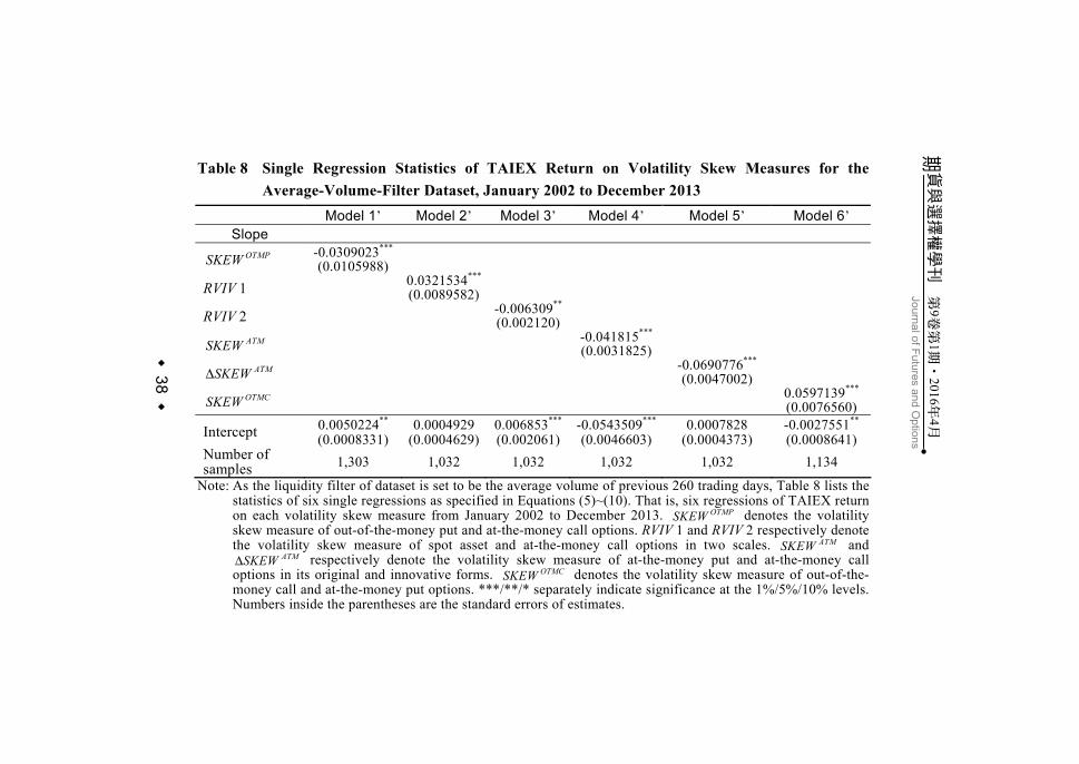
Table 8 shows the results of single regressions for the average-volume-filter dataset. We observe that all of the volatility skews are significantly related with TAIEX return at the expected directions illuminated by the literature.
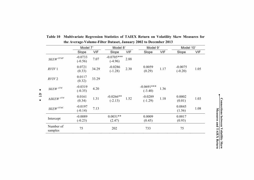
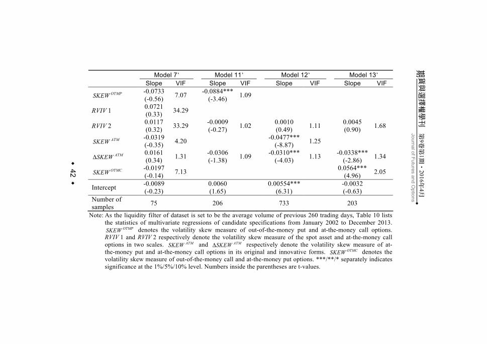
The single regression result shows that each of the six volatility skew measures is significantly correlated with TAIEX return for the zero-volume-filter dataset as well as the average-volume-filter dataset. In this subsection, we examine the collective effects of skew measures on TAIEX return by the alternative multivariate regression specifications. We follow the same criteria developed in 3.2.3 to deal with the potential collinearity problem. The alternative multivariate regression models are developed while the average-volume-filter dataset is applied. The results are summarized in Table 10. Model 7’ specified by Equation (11) in which simultaneously incorporates all six volatility skew measures. It shows that all of the six slope
37
Connections between Volatility Skew Measures and TAIEX Return ‧
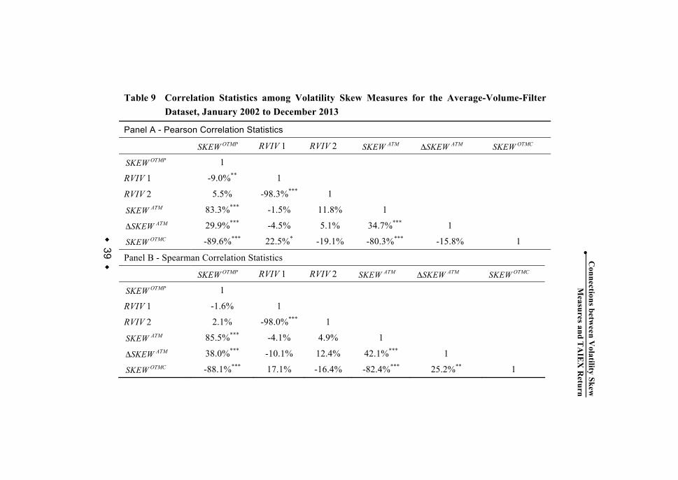
estimates are not related with TAIEX return at 10% significant level even they are not unanimously consistent with their corresponding empirical results of single regression frameworks. Therefore, it is reasonable to discard some regressors of Model 7’ to cope with the collinearity problem. Model 8’~13’ demonstrate the possible combinations of skews after allowing for the previous considerations as those specified in Table 7 in which the zero-volume-filter dataset is applied. Note that the VIFs of regressors range from 1.02 to 2.88, which are smaller than the values of VIFs in Model 7’. It indicates that the collinearity problem can be lessened in these multivariate regression models. Comparing the results of multivariate regressions where the average-volume-filter dataset is applied with the corresponding results where the zero-volume-filter dataset is applied, we observe that most of the skew measures are still significantly correlated with the spot return at the expected directions. However, we also observe that some volatility skew measures such as RVIV 1, RVIV 2, and ATMSKEW∆ impose less connection on the spot return while the average-volume-filter dataset being applied.
38
期貨與選擇權學刊
第
9卷
第1期
201‧
6年
4月
Journal of Futures and O
ptions
‧
Table 8 Single Regression Statistics of TAIEX Return on Volatility Skew Measures for the Average-Volume-Filter Dataset, January 2002 to December 2013
Model 1’ Model 2’ Model 3’ Model 4’ Model 5’ Model 6’ Slope
OTMPSKEW -0.0309023***
(0.0105988)
RVIV 1 0.0321534***
(0.0089582)
RVIV 2 -0.006309** (0.002120)
ATMSKEW -0.041815***
(0.0031825)
ATMSKEW∆ -0.0690776***
(0.0047002)
OTMCSKEW 0.0597139***
(0.0076560)
Intercept 0.0050224**
(0.0008331)0.0004929
(0.0004629)0.006853*** (0.002061)
-0.0543509***
(0.0046603) 0.0007828
(0.0004373) -0.0027551**
(0.0008641) Number of samples 1,303 1,032 1,032 1,032 1,032 1,134
Note: As the liquidity filter of dataset is set to be the average volume of previous 260 trading days, Table 8 lists the statistics of six single regressions as specified in Equations (5)~(10). That is, six regressions of TAIEX return on each volatility skew measure from January 2002 to December 2013. OTMPSKEW denotes the volatility skew measure of out-of-the-money put and at-the-money call options. RVIV 1 and RVIV 2 respectively denote the volatility skew measure of spot asset and at-the-money call options in two scales. ATMSKEW and
ATMSKEW∆ respectively denote the volatility skew measure of at-the-money put and at-the-money call options in its original and innovative forms. OTMCSKEW denotes the volatility skew measure of out-of-the-money call and at-the-money put options. ***/**/* separately indicate significance at the 1%/5%/10% levels. Numbers inside the parentheses are the standard errors of estimates.
39 ‧Connections betw
een Volatility Skew
M
easures and TA
IEX
Return
Table 9 Correlation Statistics among Volatility Skew Measures for the Average-Volume-Filter Dataset, January 2002 to December 2013
Panel A - Pearson Correlation Statistics
OTMPSKEW RVIV 1 RVIV 2 ATMSKEW ATMSKEW∆ OTMCSKEW OTMPSKEW 1
RVIV 1 -9.0%** 1
RVIV 2 5.5% -98.3%*** 1 ATMSKEW 83.3%*** -1.5% 11.8% 1
ATMSKEW∆ 29.9%*** -4.5% 5.1% 34.7%*** 1 OTMCSKEW -89.6%*** 22.5%* -19.1% -80.3%*** -15.8% 1
Panel B - Spearman Correlation Statistics
OTMPSKEW RVIV 1 RVIV 2 ATMSKEW ATMSKEW∆ OTMCSKEW OTMPSKEW 1
RVIV 1 -1.6% 1
RVIV 2 2.1% -98.0%*** 1 ATMSKEW 85.5%*** -4.1% 4.9% 1
ATMSKEW∆ 38.0%*** -10.1% 12.4% 42.1%*** 1 OTMCSKEW -88.1%*** 17.1% -16.4% -82.4%*** 25.2%** 1
40
期貨與選擇權學刊
第
9卷
第1期
201‧
6年
4月
Journal of Futures and O
ptions
‧
Note: As the liquidity filter of dataset is set to be the average volume of previous 260 trading days, Table 9 lists the correlation statistics among volatility skew measures from January 2002 to December 2013. OTMPSKEW denotes the volatility skew measure of out-of-the-money put and at-the-money call options. RVIV 1 and RVIV 2 respectively denote the volatility skew measure of the spot asset and at-the-money call options in two scales. ATMSKEW and ATMSKEW∆ respectively denote the volatility skew measure of at-the-money put and at-the-money call options in its original and innovative forms. OTMCSKEW denotes the volatility skew measure of out-of-the-money call and at-the-money put options. ***/**/* separately indicate significance at the 1%/5%/10% levels.
41 ‧Connections betw
een Volatility Skew
M
easures and TA
IEX
Return
Table 10 Multivariate Regression Statistics of TAIEX Return on Volatility Skew Measures for the Average-Volume-Filter Dataset, January 2002 to December 2013
Model 7’ Model 8’ Model 9’ Model 10’ Slope VIF Slope VIF Slope VIF Slope VIF
OTMPSKEW -0.0733 (-0.56) 7.07 -0.0705***
(-4.96) 2.88
RVIV 1 0.0721 (0.33) 34.29 -0.0286
(-1.28) 2.30 0.0059 (0.29) 1.17 -0.0075
(-0.20) 1.05
RVIV 2 0.0117 (0.32) 33.29
ATMSKEW -0.0319 (-0.35) 4.20 -0.0691***
(-3.40) 1.36
ATMSKEW∆ 0.0161 (0.34) 1.31 -0.0266**
(-2.13) 1.52 -0.0289 (-1.29) 1.18 0.0002
(0.01) 1.03
OTMCSKEW -0.0197 (-0.14) 7.13 0.0845
(1.56) 1.08
Intercept -0.0089 (-0.23) 0.0031**
(2.47) 0.0009 (0.45) 0.0017
(0.93)
Number of samples 75 202 733 75
42
期貨與選擇權學刊
第
9卷
第1期
201‧
6年
4月
Journal of Futures and O
ptions
‧
Model 7’ Model 11’ Model 12’ Model 13’ Slope VIF Slope VIF Slope VIF Slope VIF
OTMPSKEW -0.0733(-0.56) 7.07 -0.0884***
(-3.46) 1.09
RVIV 1 0.0721 (0.33) 34.29
RVIV 2 0.0117 (0.32) 33.29 -0.0009
(-0.27) 1.02 0.0010 (0.49) 1.11 0.0045
(0.90) 1.68
ATMSKEW -0.0319(-0.35) 4.20 -0.0477***
(-8.87) 1.25
ATMSKEW∆ 0.0161 (0.34) 1.31 -0.0306
(-1.38) 1.09 -0.0310*** (-4.03) 1.13 -0.0338***
(-2.86) 1.34
OTMCSKEW -0.0197(-0.14) 7.13 0.0564***
(4.96) 2.05
Intercept -0.0089(-0.23) 0.0060
(1.65) 0.00554*** (6.31) -0.0032
(-0.63)
Number of samples 75 206 733 203
Note: As the liquidity filter of dataset is set to be the average volume of previous 260 trading days, Table 10 lists the statistics of multivariate regressions of candidate specifications from January 2002 to December 2013.
OTMPSKEW denotes the volatility skew measure of out-of-the-money put and at-the-money call options. RVIV 1 and RVIV 2 respectively denote the volatility skew measure of the spot asset and at-the-money call options in two scales. ATMSKEW and ATMSKEW∆ respectively denote the volatility skew measure of at-the-money put and at-the-money call options in its original and innovative forms. OTMCSKEW denotes the volatility skew measure of out-of-the-money call and at-the-money put options. ***/**/* separately indicates significance at the 1%/5%/10% level. Numbers inside the parentheses are t-values.
43
Connections between Volatility Skew Measures and TAIEX Return ‧
4. The Impact of the 2008 Financial Tsunamis In order to consider the impact of the 2008 financial tsunamis on
the relation between the skew measures and TAIEX return, we apply the single regression models and multivariate regression models developed in the previous section to examine the relation between the volatility skew measures and TAIEX return after the financial tsunamis (2008/1-2013/12).
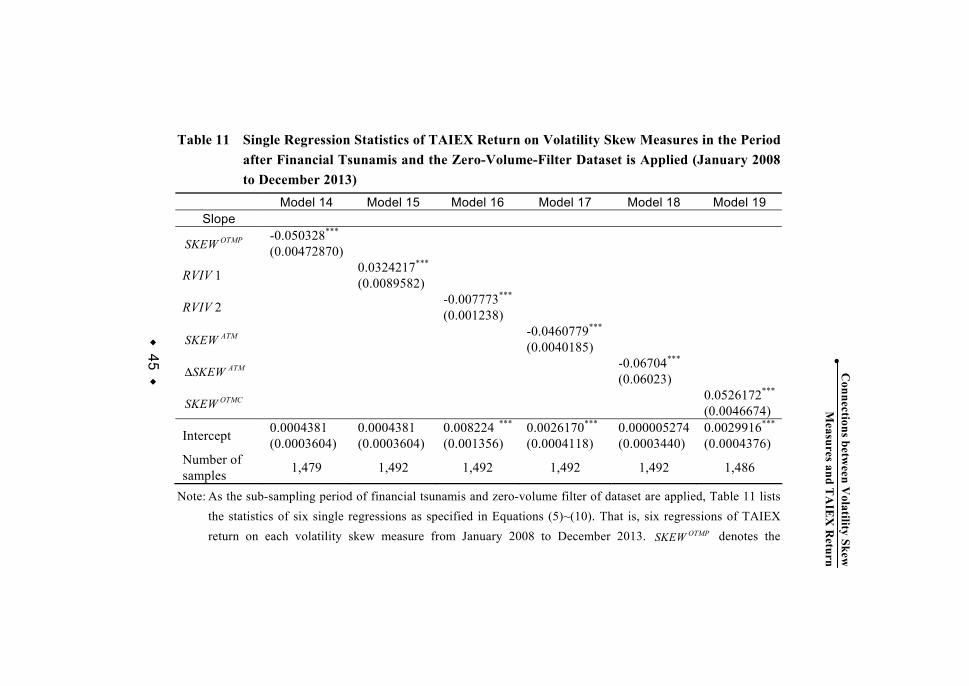
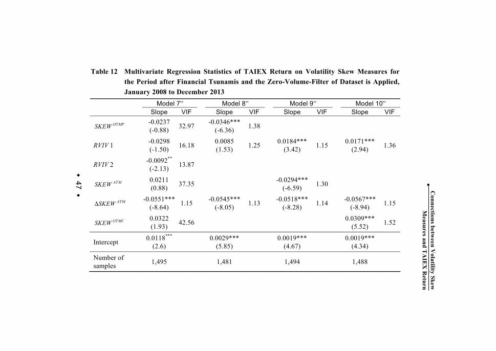
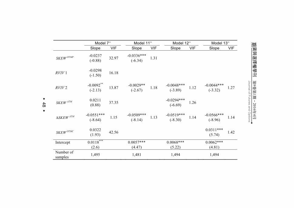
Tables 11 shows the results of single regressions after the financial tsunamis in the case of the zero-volume-filter dataset being applied. We observe that all the six skew measures are still related with spot return at 1% significant level after the financial tsunamis. The results of multivariate regressions for the period after the financial tsunamis are presented in Table 12. Model 7’’ specified in Equation (11) contains all six volatility skew measures. Model 8’’~13’’ demonstrate corresponding specifications as those specified in the former subsections. We observe that only the RVIV 1 in Model 8’’ is not statistically related with TAIEX return, the other combinations of skew measures are all correlated with TAIEX return at 1% significantly level during the period after the financial tsunamis.
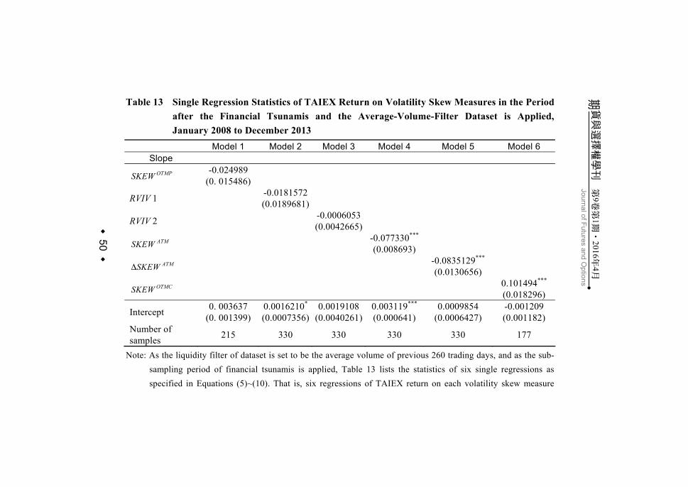
The results of single regressions and multivariate regressions during the period after the financial tsunamis while the average-volume-filter dataset being applied are presented in Tables 13 and 14, respectively. We observe that only three of the six skew measures,
ATMSKEW , ATMSKEW∆ , and OTMCSKEW , are correlated with TAIEX return at 1% significant level after the financial tsunamis. The result of multivariate regression shows that the correlation between the skew measures and TAIEX return become weaker after the financial

44
Journal of Futures and Options期貨與選擇權學刊 第9卷第1期 201‧ 6年4月
‧
tsunamis when the average-volume-filter dataset is applied. The phenomenon may be attributed to the interaction effect of volatility skews, liquidity and time-varying systematic risk on the capital markets. The issue is worth of exploring in the future.
45 ‧Connections betw
een Volatility Skew
M
easures and TA
IEX
Return
Table 11 Single Regression Statistics of TAIEX Return on Volatility Skew Measures in the Period after Financial Tsunamis and the Zero-Volume-Filter Dataset is Applied (January 2008 to December 2013)
Model 14 Model 15 Model 16 Model 17 Model 18 Model 19 Slope
OTMPSKEW -0.050328***
(0.00472870)
RVIV 1 0.0324217*** (0.0089582)
RVIV 2 -0.007773*** (0.001238)
ATMSKEW -0.0460779***
(0.0040185)
ATMSKEW∆ -0.06704***
(0.06023)
OTMCSKEW 0.0526172***
(0.0046674)
Intercept 0.0004381
(0.0003604) 0.0004381 (0.0003604)
0.008224 *** (0.001356)
0.0026170***
(0.0004118) 0.000005274(0.0003440)
0.0029916***
(0.0004376)Number of samples 1,479 1,492 1,492 1,492 1,492 1,486
Note: As the sub-sampling period of financial tsunamis and zero-volume filter of dataset are applied, Table 11 lists the statistics of six single regressions as specified in Equations (5)~(10). That is, six regressions of TAIEX return on each volatility skew measure from January 2008 to December 2013. OTMPSKEW denotes the

46
期貨與選擇權學刊
第
9卷
第1期
201‧
6年
4月
Journal of Futures and O
ptions
‧
volatility skew measure of out-of-the-money put and at-the-money call options. RVIV 1 and RVIV 2 respectively denote the volatility skew measure of spot asset and at-the-money call options in two scales.
ATMSKEW and ATMSKEW∆ respectively denote the volatility skew measure of at-the-money put and at-the-money call options in its original and innovative forms. OTMCSKEW denotes the volatility skew measure of out-of-the-money call and at-the-money put options. ***/**/* separately indicate significance at the 1%/5%/10% levels. Numbers inside the parentheses are the standard errors of estimates.
47 ‧Connections betw
een Volatility Skew
M
easures and TA
IEX
Return
Table 12 Multivariate Regression Statistics of TAIEX Return on Volatility Skew Measures for the Period after Financial Tsunamis and the Zero-Volume-Filter of Dataset is Applied, January 2008 to December 2013
Model 7” Model 8” Model 9” Model 10” Slope VIF Slope VIF Slope VIF Slope VIF
OTMPSKEW -0.0237(-0.88) 32.97 -0.0346***
(-6.36) 1.38
RVIV 1 -0.0298(-1.50) 16.18 0.0085
(1.53) 1.25 0.0184*** (3.42) 1.15 0.0171***
(2.94) 1.36
RVIV 2 -0.0092**
(-2.13) 13.87
ATMSKEW 0.0211 (0.88) 37.35 -0.0294***
(-6.59) 1.30
ATMSKEW∆ -0.0551***(-8.64) 1.15 -0.0545***
(-8.05) 1.13 -0.0518*** (-8.28) 1.14 -0.0567***
(-8.94) 1.15
OTMCSKEW 0.0322 (1.93) 42.56 0.0309***
(5.52) 1.52
Intercept 0.0118***
(2.6) 0.0029***(5.85) 0.0019***
(4.67) 0.0019***(4.34)
Number of samples 1,495 1,481 1,494 1,488
48
期貨與選擇權學刊
第
9卷
第1期
201‧
6年
4月
Journal of Futures and O
ptions
‧
Model 7” Model 11” Model 12” Model 13” Slope VIF Slope VIF Slope VIF Slope VIF
OTMPSKEW -0.0237 (-0.88) 32.97 -0.0336***
(-6.34) 1.31
RVIV 1 -0.0298 (-1.50) 16.18
RVIV 2 -0.0092**
(-2.13) 13.87 -0.0029**(-2.67) 1.18 -0.0048***
(-3.89) 1.12 -0.0044***(-3.32) 1.27
ATMSKEW 0.0211 (0.88) 37.35 -0.0294***
(-6.69) 1.26
ATMSKEW∆ -0.0551***(-8.64) 1.15 -0.0509***
(-8.14) 1.13 -0.0519*** (-8.30) 1.14 -0.0566***
(-8.96) 1.14
OTMCSKEW 0.0322 (1.93) 42.56 0.0311***
(5.74) 1.42
Intercept 0.0118***
(2.6) 0.0057***(4.47) 0.0068***
(5.22) 0.0062***(4.81)
Number of samples 1,495 1,481 1,494 1,494

49 ‧Connections betw
een Volatility Skew
M
easures and TA
IEX
Return
Note: As the sub-sampling period of financial tsunamis and zero-volume filter of dataset are applied, Table 12 lists the statistics of multivariate regressions. That is, seven regressions of TAIEX return on different combinations of volatility skew measures. OTMPSKEW denotes the volatility skew measure of out-of-the-money put and at-the-money call options. RVIV 1 and RVIV 2 respectively denote the volatility skew measure of spot asset and at-the-money call options in two scales. ATMSKEW and ATMSKEW∆ respectively denote the volatility skew measure of at-the-money put and at-the-money call options in its original and innovative forms. OTMCSKEW denotes the volatility skew measure of out-of-the-money call and at-the-money put options. ***/**/* separately indicate significance at the 1%/5%/10% levels. Numbers inside the parentheses are the standard errors of estimates.
50
期貨與選擇權學刊
第
9卷
第1期
201‧
6年
4月
Journal of Futures and O
ptions
‧
Table 13 Single Regression Statistics of TAIEX Return on Volatility Skew Measures in the Period after the Financial Tsunamis and the Average-Volume-Filter Dataset is Applied, January 2008 to December 2013
Model 1 Model 2 Model 3 Model 4 Model 5 Model 6 Slope
OTMPSKEW -0.024989
(0. 015486)
RVIV 1 -0.0181572 (0.0189681)
RVIV 2 -0.0006053 (0.0042665)
ATMSKEW -0.077330***
(0.008693)
ATMSKEW∆ -0.0835129***
(0.0130656)
OTMCSKEW 0.101494*** (0.018296)
Intercept 0. 003637
(0. 001399)0.0016210* (0.0007356)
0.0019108 (0.0040261)
0.003119***
(0.000641) 0.0009854
(0.0006427) -0.001209
(0.001182) Number of samples 215 330 330 330 330 177
Note: As the liquidity filter of dataset is set to be the average volume of previous 260 trading days, and as the sub-sampling period of financial tsunamis is applied, Table 13 lists the statistics of six single regressions as specified in Equations (5)~(10). That is, six regressions of TAIEX return on each volatility skew measure
51 ‧Connections betw
een Volatility Skew
M
easures and TA
IEX
Return
from January 2008 to December 2013. OTMPSKEW denotes the volatility skew measure of out-of-the-money put and at-the-money call options. RVIV 1 and RVIV 2 respectively denote the volatility skew measure of spot asset and at-the-money call options in two scales. ATMSKEW and ATMSKEW∆ respectively denote the volatility skew measure of at-the-money put and at-the-money call options in its original and innovative forms. OTMCSKEW denotes the volatility skew measure of out-of-the-money call and at-the-money put options. ***/**/* separately indicate significance at the 1%/5%/10% levels. Numbers inside the parentheses are the standard errors of estimates.
52
期貨與選擇權學刊
第
9卷
第1期
201‧
6年
4月
Journal of Futures and O
ptions
‧
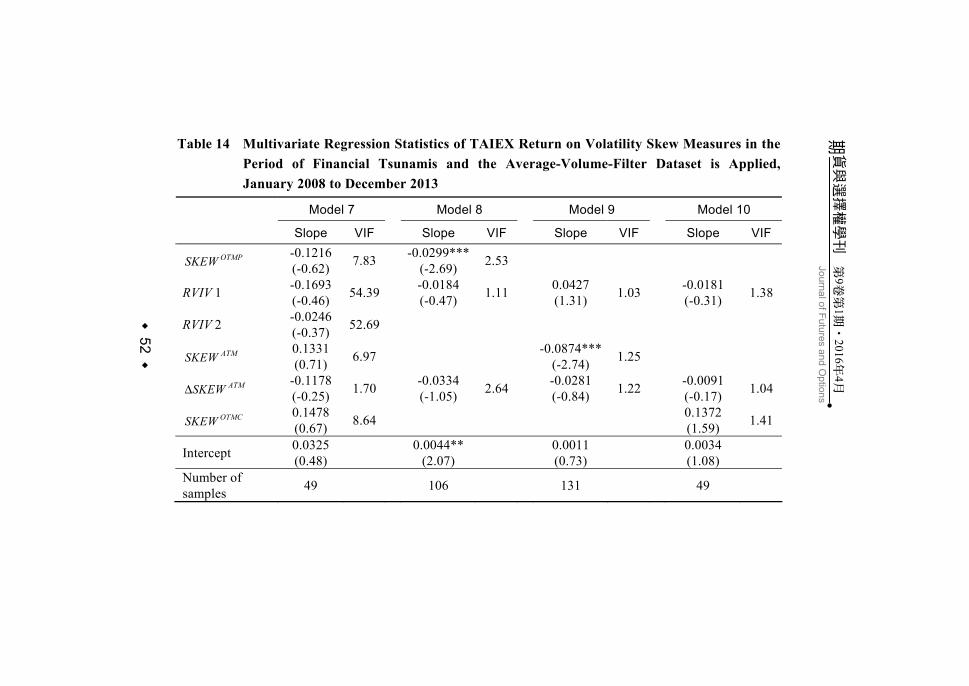
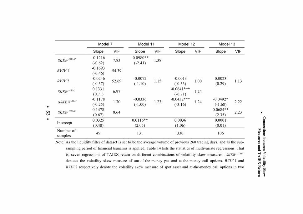
Table 14 Multivariate Regression Statistics of TAIEX Return on Volatility Skew Measures in the Period of Financial Tsunamis and the Average-Volume-Filter Dataset is Applied, January 2008 to December 2013
Model 7 Model 8 Model 9 Model 10
Slope VIF Slope VIF Slope VIF Slope VIF
OTMPSKEW -0.1216(-0.62) 7.83 -0.0299***
(-2.69) 2.53
RVIV 1 -0.1693(-0.46) 54.39 -0.0184
(-0.47) 1.11 0.0427 (1.31) 1.03 -0.0181
(-0.31) 1.38
RVIV 2 -0.0246
(-0.37) 52.69
ATMSKEW 0.1331 (0.71) 6.97 -0.0874***
(-2.74) 1.25
ATMSKEW∆ -0.1178(-0.25) 1.70 -0.0334
(-1.05) 2.64 -0.0281 (-0.84) 1.22 -0.0091
(-0.17) 1.04
OTMCSKEW 0.1478 (0.67) 8.64 0.1372
(1.59) 1.41
Intercept 0.0325
(0.48) 0.0044**(2.07) 0.0011
(0.73) 0.0034 (1.08)
Number of samples 49 106 131 49
53 ‧Connections betw
een Volatility Skew
M
easures and TA
IEX
Return
Model 7 Model 11 Model 12 Model 13
Slope VIF Slope VIF Slope VIF Slope VIF
OTMPSKEW -0.1216 (-0.62) 7.83 -0.0980**
(-2.41) 1.38
RVIV 1 -0.1693 (-0.46) 54.39
RVIV 2 -0.0246
(-0.37) 52.69 -0.0072 (-1.10) 1.15 -0.0013
(-0.33) 1.00 0.0023 (0.29) 1.13
ATMSKEW 0.1331 (0.71) 6.97 -0.0641***
(-6.71) 1.24
ATMSKEW∆ -0.1178 (-0.25) 1.70 -0.0336
(-1.00) 1.23 -0.0432*** (-3.16) 1.24 -0.0492*
(-1.68) 2.22
OTMCSKEW 0.1478 (0.67) 8.64 0.0684**
(2.35) 2.23
Intercept 0.0325
(0.48) 0.0116**(2.05) 0.0036
(1.06) 0.0001 (0.01)
Number of samples 49 131 330 106
Note: As the liquidity filter of dataset is set to be the average volume of previous 260 trading days, and as the sub-sampling period of financial tsunamis is applied, Table 14 lists the statistics of multivariate regressions. That is, seven regressions of TAIEX return on different combinations of volatility skew measures. OTMPSKEW denotes the volatility skew measure of out-of-the-money put and at-the-money call options. RVIV 1 and RVIV 2 respectively denote the volatility skew measure of spot asset and at-the-money call options in two

54
期貨與選擇權學刊
第
9卷
第1期
201‧
6年
4月
Journal of Futures and O
ptions
‧
scales. ATMSKEW and ATMSKEW∆ respectively denote the volatility skew measure of at-the-money put and at-the-money call options in its original and innovative forms. OTMCSKEW denotes the volatility skew measure of out-of-the-money call and at-the-money put options. ***/**/* separately indicate significance at the 1%/5%/10% levels. Numbers inside the parentheses are the standard errors of estimates.
55
Connections between Volatility Skew Measures and TAIEX Return ‧
IV. Conclusion
Call and put contracts can satisfy traders’ investing demands when coping with different expectation scenarios conditional on their asymmetric risk attitudes. On the other hand, the no-arbitrage argument connects option and spot markets in a natural way. However, some favorable frictions make investors tend to trade and reveal their private information in the option market instead of or prior to their corresponding operation in the spot market. All these merits endow the option market with a price discovery function relative to the spot market. Consequently, it is interesting to probe into the connection between the two markets.
Information contents of such a connection can be detected or proxied not only by price or return series, but also by volatility measures. This study is one of the few to examine the Taiwan markets in terms of volatility measures. Six skew measures consisting of realized and implied volatilities with the moneyness consideration are applied to address this issue. The TAIEX return is regressed on these measures under the frameworks of single and multivariate regressions allowing for the collinearity problem.
This study emphasizes the role of risk factor of these skew measures play on the spot return, there is no profitable trading strategy is developed. We hope that more relevant studies can be seen in the future. However, the empirical results show significant evidence that the option and spot markets connect with each other, and their relationships are consistent with the expected directions as explained

56
Journal of Futures and Options期貨與選擇權學刊 第9卷第1期 201‧ 6年4月
‧
in the literature, even under the scenarios of different liquidity filters or different sampling periods.
Specifically, when the perception of bearish/bullish events arises, the skew measures of the implied volatilities of puts and calls in the option market become higher/lower, or the skew measures of the realized volatility in the spot market and implied volatility in the option market become smaller/larger, and the spot market becomes more pessimistic/optimistic and performs poorly/well. These results apply for option contracts of different moneyness types, liquidity filters, and different sampling periods. The findings suggest that investors can exploit the volatility information of both markets for various investment demands in dealing with their equity positions.
57
Connections between Volatility Skew Measures and TAIEX Return ‧
References
Bakshi, Gurdip and Nikunj Kapadia (2003a), “Delta-Hedged Gains and the Negative Volatility Risk Premium,” Review of Financial Studies, 16, 527-566. Bakshi, Gurdip and Nikunj Kapadia (2003b), “Volatility Risk Premiums Embedded in Individual Equity Options,” Journal of Derivatives, 11, 45-54. Bali, Turan G. and Armen Hovakimian (2009), “Volatility Spreads and Expected Stock Returns,” Management Science, 55, 1797-1812. Baltussen, Guido, Bart van der Grient, Wilma de Groot, Erik Hennink and Weili Zhou (2012), “Exploiting Option Information in the Equity Market,” Financial Analysts Journal, 68, 56-72. Banerjee, Prithviraj S., James S. Doran and David R. Peterson (2007), “Implied Volatility and Future Portfolio Returns,” Journal of Banking and Finance, 31, 3183-3199. Benninga, Simon (1989), Numerical Techniques in Finance, Cambridge, MA: The MIT Press. Black, Fischer (1975), “Fact and Fantasy in the Use of Options,” Financial Analysts Journal, 31, 36-41. Bollen, Nicolas P. B. and Robert E. Whaley (2004), “Does Net Buying Pressure Affect the Shape of Implied Volatility Functions?” Journal of Finance, 59, 711-753. Buraschi, Andrea and Jens Jackwerth (2001), “The Price of a Smile: Hedging and Spanning in Option Markets,” Review of Financial Studies, 14, 495-527. Chakravarty, Sugato, Huseyin Gulen and Stewart Mayhew (2004), “Informed Trading in Stock and Option Markets,” Journal of
58
Journal of Futures and Options期貨與選擇權學刊 第9卷第1期 201‧ 6年4月
‧
Finance, 59, 1235-1258. Chan, Chin-Horng and Chieh-Jen Shih (2005), “Price Discovery in Taiwan Stock Index Derivatives Markets,” Taiwan Banking, and Finance Quarterly, 6, 31-51. Cremers, Martijn and David Weinbaum (2010), “Deviations from Put-Call Parity and Stock Return Predictability,” Journal of Financial and Quantitative Analysis, 45, 335-367. Duffie, Darrell (1996), Dynamic asset Pricing Theory, New Jersey: Princeton University Press. Frijns, Bart, Christian Tallau and Alireza Tourani-Rad (2010), “The Information Content of Implied Volatility: Evidence from Australia,” Journal of Futures Markets, 30, 134-155. Fleming, Jeff, Barbara Ostdiek and Robert E. Whaley (1996), “Trading Costs and the Relative Rates of Price Discovery in Stock, Futures, and Option Markets,” Journal of Futures Markets, 16, 353-387. Gârleanu, Nicolae, Lasse Heje Pedersen and Allen M. Poteshman (2009), “Demand-Based Option Pricing,” Review of Financial Studies, 22, 4259-4299. Goyal, Amit and Alessio Saretto (2009), “Cross-Section of Option Returns and Volatility,” Journal of Financial Economics, 94, 310-326. Hasbrouck, Joel (1995), “One Security, Many Markets: Determining the Contributions to Price Discovery,” Journal of Finance, 50, 1175-1199. Hong, Harrison and Jeremy C. Stein (1999), “A Unified Theory of Underreaction: Momentum Trading, and Overreaction in Asset Markets,” Journal of Finance, 54, 2143-2184.
59
Connections between Volatility Skew Measures and TAIEX Return ‧
Hong, Harrison, Walter Torous and Rossen Valkanov (2007), “Do Industries Lead Stock Markets?” Journal of Financial Economics, 83, 367-396. Kahneman, Daniel and Amos Tversky (1979), “Prospect Theory: An Analysis of Decision under Risk,” Econometrica, 47, 263-292. Lien, Donald and Keshab Shrestha (2009), “A New Information Share Measure,” Journal of Futures Markets, 29, 377-395. Lien, Donald and Keshab Shrestha (2014), “Price Discovery in Interrelated Markets,” Journal of Futures Markets, 34, 203-219. Xie, Shiqing and Taiping Mo (2014), “Index Futures Trading and Stock Market Volatility in China: A Difference-in-Difference Approach,” Journal of Futures Markets, 34, 282-297. Xing, Yuhang, Xiaoyan Zhang and Rui Zhao (2010), “What does Individual Option Volatility Smirk Tell us about Future Equity Returns?” Journal of Financial and Quantitative Analysis, 45, 641-662.

槓桿型與反向型ETF長短期追蹤績效之研究
61
‧
槓桿型與反向型ETF長短期 追蹤績效之研究
An Investigation of Short- and Long-term Tracking Performance of Leveraged and
Inverse ETFs
蘇亭丰* Ting-Feng Su
* 國立臺灣大學管理學院財務金融研究所。
Graduate Institute of Finance, College of Management, National Taiwan University
投稿日期:2015年11月3日;第一次修訂:2016年3月6日;接受刊登日:
2016年3月9日 Received: Nov. 3, 2015; First Revision: Mar. 6, 2016; Accepted: Mar. 9, 2016

62
Journal of Futures and Options期貨與選擇權學刊 第9卷第1期 201‧ 6年4月
‧
要 目
壹、緒 論 一、研究背景
(一) 全 球 槓 桿 型 反 向 型
ETF發展概況 (二) 臺 灣 槓 桿 型 反 向 型
ETF架構 二、研究動機與目的 三、研究架構與流程
貳、文獻探討 一、 槓桿型反向型ETF長短
期報酬相關研究 二、 每日重新平衡機制相關
研究 三、 重新平衡頻率影響追蹤
誤差相關研究 參、研究方法與實證模型
一、 槓桿型反向型ETF長短
期追蹤績效 二、 模擬不同動態調整週期
之單日追蹤績效 肆、資料來源
一、資料期間及樣本 二、資料來源
伍、研究結果與分析 一、 槓桿型反向型ETF長短
期追蹤績效評估 二、 不同動態調整週期之單
日追蹤績效模擬結果 三、 影響追蹤績效的可能
因素 (一) 期貨為標準化契約,規
格僵固且有基差風險 (二) 手續費與基金經理人議
價能力有關 (三) 現金餘額占投資組合淨
值比例 (四) 複利效果與樣本期間標
的指數走勢路徑相依 (五) 投資工具的標的指數與
槓桿型反向型ETF的標
的指數不同 陸、結 論

槓桿型與反向型ETF長短期追蹤績效之研究
63
‧
摘 要
本文研究分為兩部分。第一部分以臺灣上市的4檔槓桿型反
向型ETF為研究對象,檢驗其長短期追蹤績效。在1%顯著水準
下,4檔基金單日追蹤績效都顯著異於基金投資目標,長天期報
酬均顯著偏離標的指數目標倍數報酬。4檔槓桿型反向型ETF的持有期間累積報酬在1%顯著水準下均沒有顯著不對稱性。
第二部分以滿足所需曝險量跟淨值限制自行配置的投資組
合進行不同調整週期的動態調整機制模擬,雖然所有組合單日
報酬均顯著異於指數單日目標倍數報酬,但以剩餘現金最少之
整數解配置的組合追蹤2倍槓桿報酬績效最好,且比目前臺灣的
2檔2倍槓桿型ETF單日追蹤績效都來得佳。 期貨的基差風險及規格僵固,基金經理人對手續費之議價
能力,剩餘現金占投資組合比重大小,對標的指數的路徑相依
性,以及投資工具的標的指數與槓桿型反向型ETF所追蹤的標的
指數是否一致,皆會影響追蹤績效。
關鍵詞:槓桿型ETF、反向型ETF、追蹤績效、重新平衡機制
64
Journal of Futures and Options期貨與選擇權學刊 第9卷第1期 201‧ 6年4月
‧
Abstract
This paper is composed of two parts. The first part of the paper examines long-term and short-term tracking performances of four leveraged and inverse ETFs listed on the stock exchange in Taiwan. At 1% level of significance, daily tracking performance of the leveraged and inverse ETFs significantly deviate from the investment objectives of the funds. The cumulative returns of the leveraged and inverse ETFs over holding period are also significantly different from positive or negative multiple of cumulative returns of underlying index over corresponding period. There are no significant asymmetry in positive and negative returns.
The second part simulates the dynamic rebalancing mechanism of leveraged and inverse ETFs using different length of adjustment period on portfolios subject to needed exposure and net asset value constraints. Although daily returns of all of the portfolios dynamically rebalanced on any length of period basis are significantly different from multiple of index daily return, the portfolio allocated by the integer solution with minimized cash amount tracking two times underlying index daily return performs better than the leveraged ETFs of Taiwan.
The basis risk and standardization of futures, the bargaining power of fund managers, the percentage of cash amount that takes up, path dependence on underlying index and whether underlying index of investment vehicle is consistent with that of

槓桿型與反向型ETF長短期追蹤績效之研究
65
‧
leveraged and inverse ETFs can affect tracking performances of leveraged and inverse ETFs.
Keywords: Leveraged ETF, Inverse ETF, Tracking Performance, Rebalancing Mechanism
66
Journal of Futures and Options期貨與選擇權學刊 第9卷第1期 201‧ 6年4月
‧
壹、緒 論
一、研究背景 槓桿型反向型指數股票型基金(簡稱槓桿型反向型ETF),是以
追蹤標的指數單日正向或反向一定倍數的報酬表現為投資組合管
理目標,並在證券交易所上市交易的基金。 槓桿型ETF為每日追蹤標的指數收益正向倍數的ETF。如槓桿
倍數為2倍時,標的指數上漲1%,2倍槓桿型ETF追蹤上漲2%;標
的指數下跌1%,2倍槓桿型ETF也追蹤下跌2%。 反向型ETF則為每日追蹤標的指數報酬反向表現之ETF。如反
向倍數為1倍時,標的指數上漲1%,反向型ETF追蹤下跌1%;標
的指數下跌1%,反向型ETF也反向追蹤上漲1%。
(一)全球槓桿型反向型ETF發展概況
自1993年起,市場上已經出現具槓桿倍數的共同基金。2006年6月ProShares在美國市場發行一系列槓桿型反向型ETF(分別為
ProShares Ultra ETFs及ProShares UltraShort ETFs),為全球第一批
槓桿型ETF問世。2007年,Lyxor亦於歐洲市場推出首檔當地股票
型的槓桿型反向型ETF(分別為Lyxor ETF LEVDAX及Lyxor ETF CAC 40 DAILY 2XSHT)。2009年9月,韓國 Samsung推出亞洲首
檔股票型反向型ETF(即SAMSUNG KODEX INVERSE ETF),接著
於 2010年 2月發行亞洲首檔股票型槓桿型 ETF(即 SAMSUNG KODEX LEVERAGE ETF)。2012年4月,日本開始加入這個行
列,推出第一檔由Simplex管理之股票型槓桿ETF(即SIMPLEX TOPIX BULL 2X ETF)。日本在2012年推出後,槓桿型及反向型
ETF占整體ETF成交量達80%,而韓國自2009年推出至今,ETF成交量占整體市場比率更超越了20%,成為證券市場不容小覷的

槓桿型與反向型ETF長短期追蹤績效之研究
67
‧
一塊。 我國首檔槓桿型及反向型ETF──元大寶來臺灣50單日正向2
倍ETF(簡稱T50 2X)及元大寶來臺灣50單日反向一倍ETF(簡稱T50反),由元大寶來投信發行並於2014年10月31日上市,隨後富邦投
信發行之富邦上證180正向2倍ETF(簡稱上證2X)及富邦上證180反向1倍ETF(簡稱上證反)也於11月25日上市。
綜觀海內外市場上現有商品,商品的目標槓桿倍數自反向3倍到正向3倍,追蹤標的也不僅止於股權類型,也有以商品、債市、
貨幣匯率為追蹤標的之基金商品。與歐美國家相比,亞洲地區的日
本、韓國商品線相對侷限於股權商品,發行檔數也少很多。 根據Boost全球槓桿及反向型指數化商品研究報告,截至2015
年2月底,全球槓桿及反向型指數化商品合計發行檔數已有1,036檔,總資產管理規模已達616.66億美元[圖1],其中有40%為反向
型商品所持有,57%為槓桿型商品所持有,槓桿倍數以2倍槓桿的
商品最多[圖2]。
(二)臺灣槓桿型反向型ETF架構
歐美國家主要是以交換契約(swap)跟現貨的組合方式,而日
韓則是以期貨與現貨組成。我國的金融市場與法規環境跟亞洲較
為相近,因而採取日本與韓國的槓桿型反向型ETF架構,以期貨
曝險的方式,來達成基金投資管理目標。 槓桿型ETF的投資標的主要以標的指數之成分股、標的指數
之指數股票型基金與指數型基金、與標的指數具高度連結或相關
性之有價證券,以及衍生自標的指數之指數期貨、與標的指數具
高度連結或相關性之證券相關商品達到基金追求槓桿的投資目標。
反向型ETF以放空期貨的方式,建構基金整體的反向曝險部位。 T50 2X的基金持股中現貨標的包括元大寶來臺灣50 ETF及臺

68
Journal of Futures and Options期貨與選擇權學刊 第9卷第1期 201‧ 6年4月
‧
灣50指數少數成分股票,期貨標的大多數為臺灣證券交易所股價
指數期貨(簡稱臺股期貨),臺灣50ETF期貨為輔。市場上雖有臺灣
50指數期貨,但其成交量很小,其他各指數期貨中以臺股期貨與
臺灣50指數相關性最高[表1],其成交量最大、流動性佳[表2]。臺
灣50ETF期貨雖於2014年10月6日掛牌交易,在與標的指數相關性
及流動性等因素綜合考量之下,基金成立初期仍以交易臺股期貨
為主。T50反亦以臺股期貨為主與少部分臺灣50ETF期貨的空頭部
位實現基金反向曝險的投資目標。 上證2X的基金持股中現貨標的包括富邦上證180 ETF、上證
180指數成分股票,期貨標的大多數為新加坡交易所富時中國A50指數期貨,FB上證ETF期貨為輔。國內市場沒有直接衍生自上證
180指數的期貨商品,而FB上證ETF期貨雖於2014年10月6日掛牌
交易,流動性尚待觀察,故基金成立初期的期貨標的交易新加坡
交易所的富時中國A50指數期貨為主。上證反亦以放空新加坡交
易所富時中國A50指數期貨與少部分FB上證ETF期貨進行基金反
向曝險。 基金追蹤標的指數的方式可區分為兩種類型,一種是直接追
蹤標的指數,另一種則是追蹤槓桿及反向指數。槓桿及反向指數
是由原追蹤標的指數編制而成,將標的指數之每日槓桿或反向倍
數報酬表現於指數的波動,並已反映實際投資之資金成本。 T50 2X及T50反直接追蹤臺灣50指數,上證2X及上證反則是
分別追蹤上證180兩倍槓桿指數及上證180反向指數。根據中証指
數有限公司上證180槓桿指數系列編制方案,指數成分包含標的指
數、無風險利率及賣空成本三部分,目前無風險利率參考金融機
構人民幣貸款基準利率(六個月以內),賣空成本參考國內券商融
券利率,前述無風險利率基礎上上浮3%。當市場公允的無風險利
率及賣空成本發生變化時,指數也隨之相應調整。指數計算方式

槓桿型與反向型ETF長短期追蹤績效之研究
69
‧
如(1)式: 1 , 1 ,
, (1)
It:第t日指數點位 0t
I:第t日前一交易日指數點位
L:槓桿倍數(反向為負) rsse180,t:第t日上證180指數報酬率
0,ι tr :第t日前一交易日無風險利率
0,b tr :第t日前一交易日賣空成本(正向槓桿指數不含此項)
二、研究動機與目的 槓桿型反向型ETF在國外行之有年,在各地市場推出後皆有
快速的成長,國外有許多文獻討論槓桿型反向型ETF的商品特性
及其追蹤績效的實證研究,但研究對象幾乎都是美國地區的槓桿
型反向型ETF。臺灣追蹤主要指數的ETF商品已臻完備,在2014年底隨著法規的開放開始推出槓桿型反向型ETF,不僅為臺灣ETF市場注入新的活水,更提供國內投資人另一個投資指數的新選擇。
目前臺灣不乏對ETF追蹤績效的研究,幾乎沒有槓桿型反向
型ETF的研究,即使有,研究對象也是美國市場的商品。臺灣槓
桿型反向型ETF上市至今已有半年,目前尚無研究檢驗其長短期
追蹤績效,且槓桿型反向型ETF理論上須每日動態調整曝險,但
調整時衍生之交易費用會侵蝕ETF獲利,倘若改變調整週期,會
如何影響基金的追蹤績效更有待討論。 本文以臺灣4檔槓桿型反向型ETF為研究對象,檢驗基金上市
日起到2015年3月31日的報酬表現,另外自行模擬不同調整週期的
投資組合,同樣追蹤標的指數目標倍數日報酬,再與臺灣4檔槓桿

70
Journal of Futures and Options期貨與選擇權學刊 第9卷第1期 201‧ 6年4月
‧
型反向型ETF比較。研究目的如下: (一)檢驗基金單日追蹤績效是否達到基金投資目標,長天期
累積報酬是否還有同樣的倍數效果。 (二)自行模擬投資組合,比較不同動態調整週期的投資組合
單日報酬追蹤績效。
三、研究架構與流程 本文研究架構依序為:第一部分敘述研究背景、研究動機與
目的、研究架構和流程,第二部分回顧相關文獻研究,第三部分
說明研究方法與實證模型,第四部分說明資料樣本及來源出處,
第五部分分析研究結果,第六部分針對實證結果作整合性結論。
貳、文獻探討
一、槓桿型反向型ETF長短期報酬相關研究 槓桿型反向型ETF所提供之倍數報酬或反向報酬均以單日為
基準,超過一日會因複利效果,報酬率可能偏離基金投資目標,
適合短期操作,不適合長期持有。 下面以2天期為例,說明報酬的複利效果。定義 、 、 分
別為標的指數、兩倍槓桿型ETF、一倍反向型ETF時間t時單日報
酬率, 、 、 為標的指數、2倍槓桿型ETF、一倍反向型
ETF時間t+2時累積兩日報酬率。 2 (2) (3) 1 1 1 (4)
槓桿型與反向型ETF長短期追蹤績效之研究
71
‧
1 2 1 2 1 2 2 4 (5) 1 1 1 (6) 2 2 (7) 2 (8)
由上述式子推導,得知槓桿型反向型ETF累積兩日報酬已偏
離標的指數報酬的2倍,持有時間越長,複利效果對於槓桿型反向
型ETF累積報酬偏離指數之倍數累積報酬的影響越大,偏離方向
則無法預估。若標的指數發生連續性上漲或連續下跌,0,槓桿型反向型ETF報酬表現會超過(outperform)指數目標倍數報
酬;若標的指數發生上下震盪, 0,槓桿型反向型ETF報酬表現不如(underperform)指數目標倍數報酬。正向反向相同倍數
的槓桿型反向型ETF,反向型ETF的偏離程度比槓桿型ETF來得
大。Lu,Wang and Zhang (2009)首度對槓桿型反向型ETF長天期
報酬表現進行證研究,檢驗以Dow Jones Industrial Average、S&P 500 index、Nasdaq 100 index和Russell 2000 index為追蹤標的指數
的ProShares兩倍槓桿型反向型ETF長短期報酬,其單日追蹤績效
是否有效達到基金投資目標,一天以上的累積報酬是否還有同樣
的倍數效果。將槓桿型反向型ETF報酬對指數報酬迴歸,檢定迴
歸係數顯著性。實證結果指出,這幾檔基金單日績效雖統計上顯
著異於目標倍數但經濟意義上差距不大,反向型ETF自季報酬開
始便明顯偏離目標報酬,槓桿型ETF持有一年方才偏離。實證結
果同樣發現反向型ETF偏離程度大於同倍數槓桿型ETF。本文將以
72
Journal of Futures and Options期貨與選擇權學刊 第9卷第1期 201‧ 6年4月
‧
Lu,Wang and Zhang (2009)的實證方法為研究基礎,檢驗臺灣4檔槓桿型反向型ETF長短期追蹤績效。
然而,Lu,Wang and Zhang (2009)並未對槓桿型反向型ETF報酬行為提出一解析解。Cheng and Madhavan (2009)假設一幾何
布朗運動捕捉基金淨值變化,提出一槓桿型反向型ETF長期報酬
函數,報酬函數呈現槓桿型反向型ETF長天期報酬跟標的指數波
動度和持有期間有反向關係,指數波動度越大、持有期間越長,
報酬減損越多,槓桿型反向型ETF長天期報酬與標的指數路徑相
依(path dependence)。
二、每日重新平衡機制相關研究 槓桿型反向型ETF需依基金資產及市場現況每日計算基金所
需曝險量,每日動態調整基金投資組合,使基金整體曝險貼近基
金淨資產價值之正向或反向倍數之百分之一百。基金淨值除了受
到每日重新平衡後之投資組合價格波動之影響外,動態調整衍生
之交易稅、手續費等交易費用則會侵蝕ETF之獲利。Jarrow (2010)用普通ETF及貨幣市場帳戶(money market account)之動態組合刻劃
槓桿型反向型ETF的投資期間報酬,認為造成k倍槓桿型ETF期間
報酬與普通ETF報酬k倍不一致體現於普通ETF的波動度與資金借
貸成本有關。Avellaneda and Zhang (2010)考慮了融資成本及費用
率,將槓桿型ETF報酬表示為與融資利率(funding rate)、費用率
(expense ratio)、標的指數已實現變異數(realized variance)標的指數
報酬和借券成本(cost of borrowing shares)有關的函數,長天期報酬
的路徑相依性表現在標的指數變異數及過程中發生之融資成本及
費用。實際驗證其提出之報酬函數對槓桿型反向型ETF報酬行為
的刻劃能力,以美國56檔槓桿型反向型ETF進行實證,發現所提
出的報酬函數能良好刻劃槓桿型反向型ETF的報酬行為。

槓桿型與反向型ETF長短期追蹤績效之研究
73
‧
槓桿型反向型ETF為日報酬基金,基金管理上較傳統ETF更為
積極,每日重新平衡(daily rebalancing)機制造成槓桿型反向型ETF具有特別的市場動能。槓桿型反向型ETF每日重新平衡時,部位
調整方向跟指數變動方向一致。意即指數上漲,槓桿型反向型
ETF重新平衡時均作多;指數下跌,槓桿型反向型重新平衡時均
作空,槓桿型ETF的經理人需「買高賣低」以達到所需曝險量。
由於基金是依據標的指數收盤價來進行曝險調整,在越接近收盤
時進行動態調整會越準確,Cheng and Madhavan (2009)因此認為
每日重新平衡機制造成市場更大的買賣壓,加劇每日收盤前的波
動度,槓桿型反向型ETF甚至一度被認為是2008年金融海嘯的罪
魁禍首。 Trainor Jr. (2010)則提出證據反駁這樣的言論。觀察S&P 500
日報酬60天移動年化標準差,儘管近年槓桿型反向型ETF持續成
長,金融海嘯時異常竄升的波動度已回到海嘯前水準,波動度並
沒有系統性的升高。日內波動度在開盤後一小時和收盤前一小時
無顯著差異,雖在金融海嘯時驟升,也隨即回到海嘯前水準,因此
認為槓桿型反向型ETF的蓬勃與金融海嘯驟升的波動度純屬巧合。
三、重新平衡頻率影響追蹤誤差相關研究 Avellaneda and Zhang (2010)使用槓桿型ETF複製標的指數一
倍報酬。若槓桿倍數為β,跟傳統ETF相比僅需使用1/β的資金即
可達到複製標的指數報酬的效果。買進一單位傳統ETF同時賣出
適當單位的槓桿型ETF形成無市場風險的投資組合,分別使用定
期、根據Delta曝險變動程度兩種方式進行動態複製。若Delta曝險
變動5%以內,追蹤誤差還算合理,相應的動態調整週期可達10天以上。意即投資人若想用較少的資金,以槓桿型ETF複製標的指
數報酬,實務上不須每日如此頻繁的動態調整,追蹤誤差也尚在

74
Journal of Futures and Options期貨與選擇權學刊 第9卷第1期 201‧ 6年4月
‧
合理範圍內。 Trainor Jr. and Carroll (2013)研究槓桿型ETF長天期報酬減損
(decay)幅度與變異數、持有期間之間的關係。給定市場變異數條
件及投資人可容許的減損門檻(decay threshold),可計算投資人持
有槓桿型ETF的最長期間有多長。 上述重新平衡頻率與追蹤誤差關係的研究係以基金投資人的
角度出發,說明槓桿型反向型ETF在投資組合管理的應用,並非
對槓桿型反向型ETF基金投資組合配置,重新平衡曝險的機制作
其他調整頻率的討論。 美國Direxion發行以月報酬為單位的槓桿型共同基金,其追求
基金月報酬達標的指數月報酬之一定倍數。Little (2010)特別提醒
投資人注意月報酬槓桿型共同基金的特性,其以追求標的倍數報
酬以月為基準,因此基金經理人需每月調整曝險而非每日調整,
為降低追蹤誤差,曝險量盡量以標的指數一個月後的指數水準來
調整,因此重新調整時點越接近標的指數月報酬計算時點越好,
但會增加基金在月內發生淨值歸零的可能性。 以上文獻均未對槓桿型反向ETF此類以追求標的指數日報酬
為基金管理目標,基金投資組合動態調整頻率對追蹤績效的影響
進行研究,本文欲以基金經理人的角度出發,研究不同投資組合
動態調整頻率對基金日報酬追蹤績效的影響。
參、研究方法與實證模型
本文研究分為兩部分:第一部分檢驗臺灣4檔槓桿型反向型
ETF不同持有期間的報酬追蹤績效,第二部分檢驗以本文提出的
動態調整方法所模擬之不同調整週期的單日報酬追蹤績效。

槓桿型與反向型ETF長短期追蹤績效之研究
75
‧
一、槓桿型反向型ETF長短期追蹤績效 檢驗槓桿型反向型ETF單日報酬追蹤績效是否有效達到標的
指數之目標倍數報酬表現,並檢驗槓桿型反向型ETF持有一天以
上之長天期報酬與標的指數報酬是否存在目標槓桿倍數關係。持
有期間設定為一日、兩日、五日(週)、十日(雙週)和二十日(月),分別檢驗單日報酬、雙日報酬、週報酬、雙週報酬及月報酬的追
蹤績效。 計算持有期間報酬率採重疊數據(overlapping data)的方式計
算,樣本數喪失的最少: (9)
若計算基金報酬率,Pt為淨資產價值(NAV); 若計算指數報酬率,Pt為指數收盤價 將槓桿型反向型ETF持有期間報酬率對追蹤標的指數相應期
間報酬率進行線性迴歸,應變數為槓桿型反向型ETF期間報酬
率,自變數為追蹤標的指數期間報酬率,以T檢定檢驗斜率係數
(β)在給定的顯著水準下,是否等於其所追求之槓桿倍數。 · (10)
Yi:槓桿型反向型期間報酬率; Xi:追蹤標的指數期間報酬率 此外,為檢驗報酬的對稱性,意即報酬追蹤績效的正向效果
與負向效果是否相同,在迴歸分析中新增一自變數,追蹤標的指
數報酬率乘上虛擬變數(dummy variable)D使指數報酬率非正即0,

76
Journal of Futures and Options期貨與選擇權學刊 第9卷第1期 201‧ 6年4月
‧
再對槓桿型反向型ETF報酬率進行迴歸,以t檢定檢驗第二自變數
的迴歸係數在統計上是否顯著(異於0),若係數顯著,代表報酬有
不對稱性,反之則表示報酬正負方向的效果相同。 · + · · (11) 1 , 00 , 0
Yi:槓桿型反向型ETF期間報酬率; Xi:追蹤標的指數期間報酬率
若標的指數報酬率為正,基金報酬率的迴歸所得倍數為
;若標的指數報酬率為負,基金報酬率迴歸所得倍數為 。
二、模擬不同動態調整週期之單日追蹤績效 建構一基金投資組合模擬現有之槓桿型反向型ETF,與模擬
對象追蹤同一個標的指數,投資組合期初淨資產總價值與模擬對
象上市時總發行股數所表彰之淨資產總價值相當,採用與模擬對
象之成分相同的現貨標的及期貨標的建構投資組合,交易稅、手
續費、基金管理費、基金保管費均需列入計算,若現貨與期貨之
計價單位不同時,尚須考慮匯率的變動。起初建構投資組合時,
現貨、期貨與現金部位比例須滿足下列兩個條件,組合配置方式
非唯一解: (1)現貨曝險量+期貨曝險量/(1+一日利率)=基金所需曝險量 (2)現貨成本+期貨成本+剩餘現金=基金淨資產總價值
期貨曝險量須以一日利率折現,但一日利率微乎其微,故本
文忽略不計。投資組合需因應追蹤標的指數變動動態調整曝險大
小,本文研究採定期調整的方式,週期分別設定為1天/次、2天

槓桿型與反向型ETF長短期追蹤績效之研究
77
‧
/次、5天/次(即1週/次)、10天/次(即2週/次)、20天/次(即1月/次),原則上每次調整時僅調整期貨部位,惟投資組合內現
金不足以支付動態調整時所產生之交易費用,才對現貨部位進行
調整。投資組合剩餘現金需按日計息,資產價值為現貨部位、期
貨保證金餘額與剩餘現金加總,基金保管費、管理費每日從資產
價值按比例扣除後,方得最終淨資產價值。 將投資組合單日報酬與追蹤標的指數單日報酬作線性迴歸,
應變數為投資組合單日報酬率,自變數為追蹤標的指數單日報酬
率,以T檢定檢驗斜率係數(β)在給定的顯著水準下,是否等於所
追求之槓桿倍數,並與原槓桿型反向型ETF追蹤績效作比較。 (12)
Yi:投資組合單日報酬率;Xi:追蹤標的指數單日報酬率
肆、資料來源
一、資料期間及樣本 本文以元大寶來臺灣50單日正向2倍投資信託基金(簡稱T50
2X)、元大寶來臺灣50單日反向1倍投資信託基金(簡稱T50反)、富
邦上證180單日正向2倍證券投資信託基金(簡稱上證2X)、富邦上
證180單日反向1倍證券投資信託基金(簡稱上證反),4檔槓桿型反
向型ETF為研究對象[表3]。資料期間自基金上市日前一日起至
2015年3月31日為止,T50 2X及T50反自2014年10月30日起,共
101個日資料樣本數;上證2X及上證反自2014年11月24日起,共
84個日資料樣本數。 第一部分槓桿型反向型ETF長短期追蹤績效的研究,以臺灣
50指數、上證180兩倍槓桿指數及上證180反向指數收盤價計算標

78
Journal of Futures and Options期貨與選擇權學刊 第9卷第1期 201‧ 6年4月
‧
的指數報酬率,以4檔槓桿型反向型ETF每日淨資產價值計算基金
報酬率。 第二部分以不同調整週期自行模擬之投資組合單日追蹤績效
的研究,現貨以ETF每日淨資產價值、期貨以每日收盤價作為買
賣價格。以臺灣50指數為追蹤標的指數的投資組合,現貨標的採
用元大寶來臺灣50 ETF(簡稱0050),期貨標的採用臺灣證券交易
所股價指數期貨(簡稱臺股期貨);分別以上證2倍槓桿指數及上證
180反向指數為追蹤標的指數的投資組合,現貨標的採用富邦上證
180 ETF(簡稱FB上證),期貨標的採用新加坡交易所富時中國A50指數期貨(簡稱A50期貨),由於上證2X與上證反每日基金淨資產
價值是以新臺幣計算,每日曝險部位是依照淨值變動進行調整,
若幣別轉換之匯率發生變化時,將影響以新臺幣計算之基金淨資
產價值,進而影響基金的曝險量,故期貨契約價值需以美元匯率
轉換成新臺幣才能計入淨資產價值。現金以臺灣再買回利率(repo rate)按日計息,每日調整以隔夜RP利率計算,調整週期2天/次、
1週/次、2週/次以1-10天期RP利率計算,調整週期1月/次以
11-20天期RP利率計算[表4]。
二、資料來源 T50 2X、T50反、上證2X、上證反、0050,及FB上證的每日
淨資產價值,臺灣50指數收盤價,臺股期貨收盤價,臺灣再買回
利率(repo rate)及美元匯率均整理自臺灣經濟新報(TEJ)資料庫;上
證180兩倍槓桿指數及上證180反向指數收盤價整理自公開資訊觀
測站及中證指數公司網站;A50期貨收盤價則整理自Bloomberg。4檔槓桿型反向型ETF基本資料及基金成分參考自元大寶來投信、
富邦投信及臺灣證券交易所網站。
槓桿型與反向型ETF長短期追蹤績效之研究
79
‧
伍、研究結果與分析
一、槓桿型反向型ETF長短期追蹤績效評估 將槓桿型反向型ETF持有期間報酬率(應變數)對追蹤標的指數
期間報酬率(自變數)進行迴歸後,以T檢定對斜率係數做檢定。 T50 2X追蹤臺灣50指數單日正向兩倍報酬,檢定假設為: : 2 . . : 2 (13)
迴歸結果 之t統計量為:
(14)
T50反追蹤臺灣50指數單日反向1倍報酬,檢定假設為: : 1 . . : 1 (15)
迴歸結果 之t統計量為: (16)
[圖3]、[圖4]分別為樣本期間臺灣50指數與T50 2X、T50反淨
值之長短期報酬率走勢圖。如圖所示,T50 2X和T50反淨值報酬
率都沒有十分貼合臺灣50目標倍數報酬。由[表5]報酬率迴歸結果
得知,2檔基金追蹤臺灣50指數正負倍數的表現皆不如預期。無論
持有期間多長,2檔基金報酬率的迴歸斜率係數β在1%顯著水準下
皆顯著異於目標倍數,表示基金長短期報酬率均偏離正向2倍或負
向1倍於標的指數相應期間的表現。T50 2X與T50反淨值報酬率對
臺灣50指數目標倍數報酬率反應不足(undershoot)。

80
Journal of Futures and Options期貨與選擇權學刊 第9卷第1期 201‧ 6年4月
‧
上證2X追蹤的是上證180兩倍槓桿指數,上證反則是追蹤上
證180反向指數,此兩種指數的編制已反映上證180指數單日之正
向兩倍及反向1倍表現,故檢定假設為: : 1 . . : 1 (17)
迴歸結果 之t統計量為:
(18)
[圖5]為樣本期間上證180指數、上證180兩倍槓桿指數與上證
2X淨值之長短期報酬率走勢圖,[圖6]則為樣本期間上證180指數、上證180反向指數與上證反之淨值長短期報酬率走勢圖。如圖
所示,上證2X和上證反的淨值報酬率都沒有十分貼合上證180兩倍槓桿指數或反向指數的報酬率。由[表6]報酬率迴歸結果得知,
2檔基金追蹤上證180槓桿指數與反向指數的表現皆不如預期。無
論持有期間多長,2檔基金報酬率的迴歸斜率係數β在1%顯著水準
下皆顯著異於1,表示基金長短期報酬率均偏離上證180槓桿及反
向指數相應期間的表現。上證2X與上證反淨值報酬率對上證180指數目標倍數報酬率反應過度(overshoot)。
檢驗報酬不對稱性,將槓桿型反向型ETF報酬率(應變數)對「標的指數報酬率」(自變數1)與「非正即0的指數報酬率」(自變
數2)進行迴歸後,以T檢定檢定自變數1的迴歸係數 是否顯著異
於目標倍數, 是否顯著異於0。 T50 2X的 檢定假設及迴歸結果 之t統計量為: : 2 . . : 2 (19) (20)
槓桿型與反向型ETF長短期追蹤績效之研究
81
‧
T50反的 檢定假設及迴歸結果 之t統計量為: : 1 . . : 1 (21)
(22)
上證2X、上證反的 檢定假設及迴歸結果 之t統計量皆為: : 1 . . : 1 (23)
(24)
以T檢定檢定所有自變數2的迴歸係數 是否顯著異於0,檢
定假設為: : 0 . . : 0 (25)
迴歸結果 之t統計量為:
(26)
[表7]為4檔槓桿型反向型ETF對稱性迴歸結果。T50 2X和T50反在1%顯著水準下,無論持有期間長短, 均顯著異於目標倍
數,表示T50 2X和T50反追蹤臺灣50指數的績效不佳。T50反的週
報酬和月報酬 分別在10%和5%顯著水準下出現顯著不對稱性:
臺灣50指數發生正報酬時T50反的淨值跌幅比指數負報酬時的淨值
漲幅小,雖有利於基金投資人,但是偏離基金的投資目標。 上證2X單日報酬和雙日報酬的 在1%顯著水準下顯著異於
1,持有期間超過一週之報酬的 在三種顯著水準下皆不顯著異於
1;上證反在1%顯著水準下,無論持有期間長短, 均顯著異於
82
Journal of Futures and Options期貨與選擇權學刊 第9卷第1期 201‧ 6年4月
‧
1。表示尚可預期上證2X持有一週以上之報酬相當於上證180兩倍
槓桿指數同期間報酬,但上證反的長短期報酬皆偏離上證180反向
指數同期間報酬。上證2X、上證反的週報酬 在10%顯著水準下
出現顯著不對稱性:180兩倍指數上漲(上證180指數上漲)時上證
2X的淨值漲幅比起180兩倍指數下跌(上證180指數下跌)時的淨值
跌幅大,對投資人有利;180反向指數下跌(上證180指數上漲)時,上證反淨值跌幅比起180反向指數上漲(上證180指數下跌)時的淨值漲幅大,對投資人較不利,但兩者皆偏離基金投資目標。
二、不同動態調整週期之單日追蹤績效模擬結果 模擬追蹤正向2倍臺灣50指數報酬,投資組合現貨標的採用元
大寶來臺灣50 ETF,期貨標的採用臺灣股價指數期貨。假設X為現
貨單位數,Y為期貨單位數,Z為剩餘現金,參考投資標的交易規格
並考慮交易費用及基金管理費用,X、Y、Z須滿足(27)、(28)式: 1000 · 200 · 2 · (27) 1000 1 0.1425% · 83000 200 · 0.002% 60 · 1 % . % (28)
P:0050 ETF淨值 F:臺股期貨收盤價 NAV:T50正2上市前一日淨值
(X,Y,Z)配置方式非唯一解,本文以三種組合進行不同調整週
期的報酬模擬:剩餘現金最多的全期貨部位(0,1364),剩餘現金最
少的整數解(17740,716),將現金最少整數解之半數現貨換成期貨
(8870,1040)的剩餘現金居中。 [表8]為追蹤臺灣50指數的正向2倍日報酬之模擬投資組合單
日報酬追蹤績效結果,檢定假設及t統計量計算如(13)、(14)式。
槓桿型與反向型ETF長短期追蹤績效之研究
83
‧
無論調整週期多長,三種投資組合日報酬率對臺灣50指數日報酬
率迴歸的斜率係數β均顯著異於正向 2倍,報酬率反應不足
(undershoot)。調整週期而言,三種投資組合均以1週/次的追蹤
績效最好。配置方式而言,剩餘現金最少之整數解所配置的投資
組合β最接近2,在五種調整週期下的追蹤績效均比T50 2X佳。 T50反是完全由期貨組成之基金,故本文模擬追蹤反向1倍臺
灣50指數報酬的投資組合亦完全用臺灣股價指數期貨操作,期貨口
數需滿足所需曝險量且總交易成本不能超過基金淨資產總價值。 [表9]為追蹤臺灣50負向1倍日報酬之模擬投資組合單日報酬
追蹤績效結果,檢定假設及t統計量計算如(15)、(16)式。無論調
整週期多長,投資組合日報酬率對臺灣50指數日報酬的斜率係數β均顯著異於負向1倍,報酬率反應不足(undershoot)。用本文調整
方法模擬的追蹤績效,在五種調整週期下均比T50反佳,以2週/
次調整的效果尤佳。 模擬追蹤上證180兩倍槓桿指數報酬,投資組合現貨標的採用
富邦上證180 ETF,期貨標的採用新加坡交易所富時中國A50指數
期貨。參考投資標的交易規格並考慮交易費用、基金管理費用及
匯率,X、Y、Z須滿足(29)、(30)式: 1000 · · · 2 · (29) 1000 · 1 0 0.1425% 1210 0 2.7 · · 1 . % . % (30)
P:FB上證ETF淨值 F:A50期貨收盤價 NAV:上證2X上市前一日淨值 fx:美元匯率
(X,Y,Z)配置方式非唯一解,本文以三種組合進行不同調整週
期的報酬模擬:剩餘現金最多的全期貨部位(0,5748),剩餘現金最

84
Journal of Futures and Options期貨與選擇權學刊 第9卷第1期 201‧ 6年4月
‧
少的整數解(24418,3405),將現金最少整數解之半數現貨換成期貨
(12209,4575)的剩餘現金居中。 [表10]為追蹤上證180兩倍槓桿指數日報酬之模擬投資組合單
日報酬追蹤績效結果,檢定假設及t統計量計算如(17)、(18)式。
無論調整週期多長,三種投資組合日報酬率與上證180兩倍槓桿指
數日報酬率均有顯著差異,報酬率過度反應(overshoot)。調整週
期而言,三種投資組合均以1日/次的偏離程度最大,1月/次偏
離程度最小,推論投資組合動態調整頻率不能太高。配置方式而
言,剩餘現金最少之整數解所配置的投資組合β最接近1,在五種
調整週期下的追蹤績效均比上證2X佳;全期貨組合的調整週期若
長達1月/次、現金最少整數解半數現貨換期貨組合調整週期達1週/次甚或更久,績效可優於上證2X。
上證反是完全由期貨組成之基金,故本文模擬追蹤上證180反向指數報酬的投資組合亦完全用新加坡富時中國A50指數期貨操
作,期貨口數需滿足所需曝險量且總交易成本不能超過基金淨資
產總價值。 [表11]為追蹤上證180反向指數日報酬之模擬投資組合單日報
酬追蹤績效結果,檢定假設及t統計量計算如(17)、(18)式。無論
調整週期多長,投資組合日報酬率均顯著異於上證180反向指數日
報酬率,報酬率反應過度(overshoot)。用本文調整方法模擬的追
蹤績效皆比上證反差,其中以每日調整的偏離程度最小,若調整
週期拉長,報酬追蹤的效果越差。
三、影響追蹤績效的可能因素
(一)期貨為標準化契約,規格僵固且有基差風險
由於臺灣槓桿型反向型ETF商品架構與歐美不同,造成追蹤
誤差的因素可能也與歐美國家的追蹤績效影響因素不盡相同。歐

槓桿型與反向型ETF長短期追蹤績效之研究
85
‧
美主要用交換契約(swap)曝險,根據過去文獻的實證結果,歐美
商品之追蹤績效良好,甚至持有期間長達一季還能保有原先日報
酬所要求的槓桿倍數效果。臺灣商品採用期貨(futures)曝險,期貨
本身即有基差風險,且期貨為標準化商品,不像交換契約可以量
身訂做契約的曝險量,這可能會使臺灣槓桿型反向型ETF追蹤績
效比歐美的商品追蹤績效差。
(二)手續費與基金經理人議價能力有關
造成自行模擬的投資組合和臺灣4檔基金的績效差異的原因,
一部分可能來自於部位調整時所發生之交易成本。本文模擬的投
資組合,買賣現貨之手續費以最高上限0.1425%計算,T50 2X和
上證2X皆使用自己公司發行之ETF當作現貨標的,手續費在實務
上可能比0.1425%低;期貨下單時,期貨商收取的手續費在實務上
是以議價方式決定,且法人與散戶的手續費率也不同。本文模擬
的投資組合是以法人身分買賣,臺股期貨手續費以一口60元計
算,中國A50指數期貨手續費以一口2.7美元計算,更會因基金經
理人的議價能力(bargaining power)有所差異。
(三)現金餘額占投資組合淨值比例
無論是以臺灣50指數或是上證180兩倍槓桿指數為追蹤標的,
並且滿足曝險量及淨值限制下所模擬的動態調整結果,均以剩餘
現金最少之整數解組合的追蹤績效最佳,全期貨組合的追蹤績效
最差。 推測原因可能跟現金餘額占投資組合淨值比例多寡有關。基
金淨值由現貨部位價值、保證金餘額及剩餘現金加總,以追蹤標
的指數報酬為目標,淨值中與標的指數報酬變動程度相當的成分
比例越高越好。現貨部位價值與保證金餘額變動率與標的指數變
動程度較接近,現金餘額則僅以再買回利率(repo rate)按日計息,

86
Journal of Futures and Options期貨與選擇權學刊 第9卷第1期 201‧ 6年4月
‧
現金餘額日報酬率與標的指數日報酬率相形之下顯得十分微小。
因此剩餘現金越少,在基金淨值的占比越小,淨值報酬率就跟指
數報酬率越相關。此外,本文僅選擇三種組合方式進行模擬,滿
足所需曝險量及淨值限制的配置方式不勝枚舉,也許還有其他配
置方式比現金最少之整數解組合的績效更好。
(四)複利效果與樣本期間標的指數走勢路徑相依
以臺灣50指數為追蹤標的,無論是T50 2X、T50反還是自行
模擬的報酬,皆對臺灣50指數倍數報酬反應不足(undershoot);與
上證180指數高度連動的2倍槓桿與反向指數為追蹤標的之上證
2X、上證反與自行模擬的報酬,皆對上證180策略指數報酬過分
反應(overshoot)。 文獻指出槓桿型反向型ETF具路徑相依性(path dependence)。
觀察臺灣50指數[圖7]和上證180指數及上證180兩倍槓桿、反向指
數[圖8]於樣本期間內每日收盤價走勢圖,發現臺灣50指數在樣本
期間內僅小幅上漲,趨勢不明顯,期間累積報酬率為7.05%,根據
(2)至(8)式所示之複利效果,漲跌互現的交叉相乘項經常為負數,
使得T50 2X與T50反基金報酬反應不足以達到指數報酬之目標倍
數;上證1 8 0指數在樣本期間內大幅度上漲,累積報酬率達
54.18%,2倍槓桿指數上漲超過120%,反向指數下跌37%,過程
中經常出現連續上漲跟連續下跌,複利效果的交叉相乘項經常為正
數,使得上證2X與上證反基金報酬反應超過指數報酬之目標倍數。
(五)投資工具的標的指數與槓桿型反向型ETF的標的指數不同
推測另一原因可能出自投資工具的標的指數與槓桿型反向型
ETF所追蹤的標的指數不同,造成投資工具的報酬率與ETF所追蹤
的指數變動不一致。 用臺灣50 ETF和臺股期貨追蹤臺灣50指數,臺灣50 ETF同是

槓桿型與反向型ETF長短期追蹤績效之研究
87
‧
追蹤臺灣50指數,但臺股期貨標的是臺灣股價指數,臺灣股價指
數成分股較多,直覺上較臺灣50指數來得穩定,當臺灣50指數產
生變動時,臺股期貨指數變動率會小於臺灣50指數變動率,若使
用臺股期貨進行1:1的臺灣50指數曝險部位調整時,曝險部位變動
率就不能完全反映臺灣50指數的變動率。 用FB上證ETF和中國A50期貨捕捉上證180指數倍數報酬,FB
上證ETF同是追蹤上證180指數,但中國A50期貨標的是上證50指數,上證180指數成分股較多,直覺上較上證50指數來得穩定,當
上證180指數產生變動時,A50期貨指數變動率會大於上證180指數變動率,因此使用A50期貨進行1:1的上證180指數曝險部位調整
時,曝險部位變動率就會過度反映上證180指數的變動率。 為驗證推論是否合理,將臺股期貨指數報酬率對臺灣50指數
報酬率作迴歸,若迴歸係數 β 1 ,可合理解釋反應不足
(undershoot);將A50期貨指數報酬率對上證180指數報酬率作迴
歸,若迴歸係數β 1,可合理解釋過分反應(overshoot)。 [表12]為迴歸結果,t統計量計算如(17)式。臺股期貨指數報
酬率對臺灣50指數報酬率迴歸係數β顯著小於1,A50期貨指數報
酬率對上證180指數報酬率迴歸係數β顯著大於1,因此合理推論投
資工具與標的指數不一致可能為槓桿型反向型ETF報酬過與不及
的原因之一。
陸、結 論
槓桿型反向型ETF所提供的正向或反向一定倍數之指數報酬
以日報酬為基準,超過一日會因複利效果而偏離原先的倍數目
標,且偏離方向無法預估。為了每日達到目標倍數報酬,槓桿型
反向型ETF需每日重新調整投資組合部位曝險,但動態調整所衍

88
Journal of Futures and Options期貨與選擇權學刊 第9卷第1期 201‧ 6年4月
‧
生的交易費用會侵蝕ETF獲利。 本文分為兩大部分。第一部分以臺灣4檔槓桿型反向型ETF為
研究對象,檢驗其長短期追蹤績效。在1%顯著水準下,4檔基金
單日追蹤績效都顯著異於基金投資目標,長天期報酬均顯著偏離
標的指數目標倍數報酬。4檔槓桿型反向型ETF期間報酬僅少部分
出現不對稱性,在1%顯著水準下均不顯著。 第二部分自行以滿足所需曝險量跟淨值限制配置投資組合,
採用不同動態調整週期進行報酬模擬。追求指數正向2倍報酬為目
標的投資組合配置方式非唯一解,本文採「全期貨部位」、「剩
餘現金最少之整數解」、「現金最少整數解之半數現貨換成期
貨」三種組合方式;追求指數反向報酬為目標的投資組合僅「全
期貨部位」一種。自行模擬追蹤標的指數正向2倍日報酬的投資組
合中,以剩餘現金最少之整數解配置的投資組合追蹤2倍槓桿報酬
的績效最好,且比T50 2X和上證2X單日追蹤績效佳,現金最少整
數解之半數現貨換期貨組合的追蹤績效次之,全期貨部位的追蹤
績效最差。自行模擬追蹤標的指數反向1倍日報酬的全期貨投資組
合的追蹤績效則是有好有壞。 推測影響追蹤績效的可能因素來自:臺灣採用期貨曝險的方
式,期貨為標準化商品,不像歐美商品的swap架構可以量身訂做
曝險量;現貨與期貨的手續費率需視基金經理人的議價能力而
定;投資組合淨值成分中,現金日報酬率僅為一日化之再買回利
率,與標的指數日報酬率相關度低,剩餘現金占組合淨值比重對
績效的影響也有很大的關係。 綜合臺灣4檔槓桿型反向型ETF跟自行模擬投資組合的結果,
用臺灣 50 ETF和臺股期貨追蹤臺灣 50指數報酬會反應不足
(Undershoot);用富邦上證180 ETF和中國A50期貨追蹤上證180指數報酬會反應過度(Overshoot)。推測原因為投資工具的標的指數
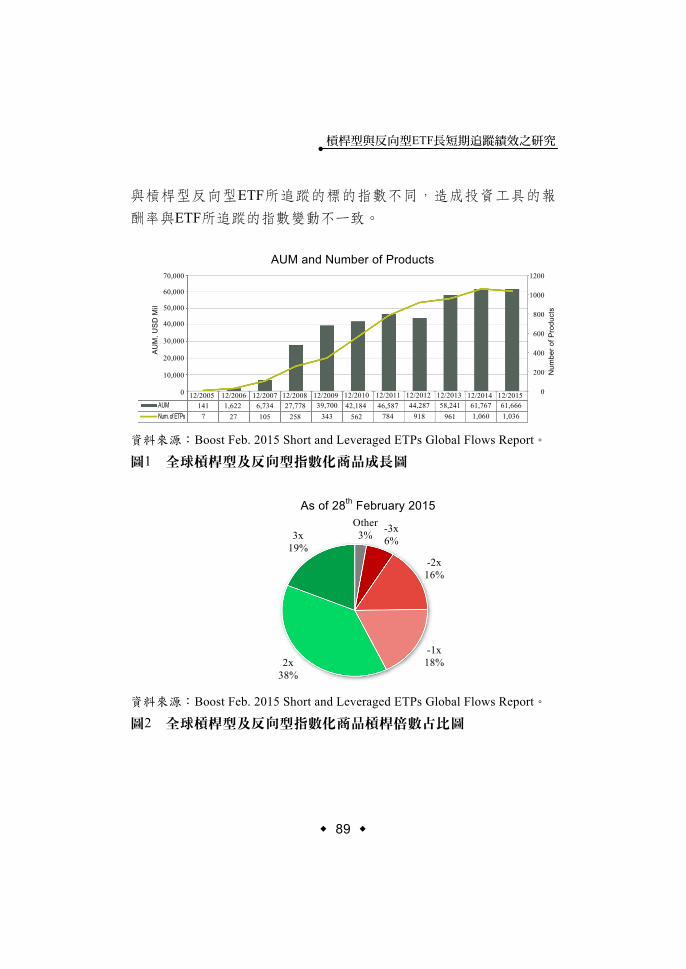
槓桿型與反向型ETF長短期追蹤績效之研究
89
‧
與槓桿型反向型ETF所追蹤的標的指數不同,造成投資工具的報
酬率與ETF所追蹤的指數變動不一致。
資料來源:Boost Feb. 2015 Short and Leveraged ETPs Global Flows Report。
圖1 全球槓桿型及反向型指數化商品成長圖
資料來源:Boost Feb. 2015 Short and Leveraged ETPs Global Flows Report。
圖2 全球槓桿型及反向型指數化商品槓桿倍數占比圖
12/2005 12/2006 12/2007 12/2008 12/2009 12/2010 12/2011 12/2012 12/2013 12/2014 12/2015 141 1,622 6,734 27,778 39,700 42,184 46,587 44,287 58,241 61,767 61,666
7 27 105 258 343 562 784 918 961 1,060 1,036 AUM Num. of ETPs
70,000
60,000
50,000
40,000
30,000
20,000
10,000
0
AU
M, U
SD
Mil
Num
ber o
f Pro
duct
s
1200
1000
800
600
400
200
0
AUM and Number of Products
As of 28th February 2015
3x19%
Other3% -3x
6%
-2x16%
2x 38%
-1x18%
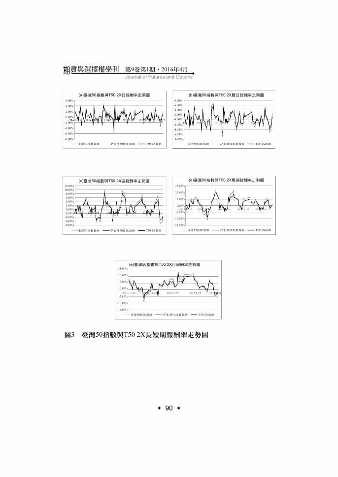
90
Journal of Futures and Options期貨與選擇權學刊 第9卷第1期 201‧ 6年4月
‧
圖3 臺灣50指數與T50 2X長短期報酬率走勢圖
(a)臺灣50指數與T50 2X日報酬率走勢圖 (b)臺灣50指數與T50 2X雙日報酬率走勢圖
(c)臺灣50指數與T50 2X週報酬率走勢圖 (d)臺灣50指數與T50 2X雙週報酬率走勢圖
……臺灣50指數報酬 2*臺灣50指數報酬 T50 2X報酬
……臺灣50指數報酬 2*臺灣50指數報酬 T50 2X報酬
……臺灣50指數報酬 2*臺灣50指數報酬 T50 2X報酬
……臺灣50指數報酬 2*臺灣50指數報酬 T50 2X報酬
……臺灣50指數報酬 2*臺灣50指數報酬 T50 2X報酬
(e)臺灣50指數與T50 2X月報酬率走勢圖 15.00%
10.00%
5.00%
0.00%
-5.00%
-10.00%
-15.00%
15.00%
10.00%
5.00%
0.00%
-5.00%
-10.00%
-15.00%
12.00%10.00%
8.00%6.00%4.00%2.00%0.00%
-2.00%-4.00%-6.00%-8.00%
6.00%
4.00%
2.00%
0.00%
-2.00%
-4.00%
-6.00%
-8.00%
8.00%6.00%4.00%2.00%0.00%
-2.00%-4.00%-6.00%-8.00%
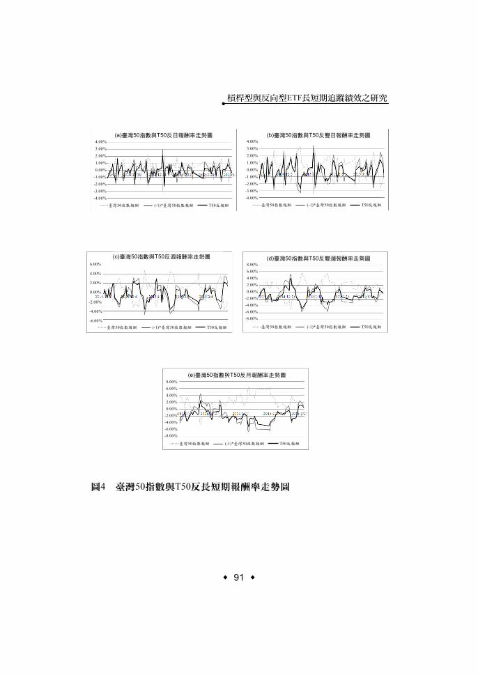
槓桿型與反向型ETF長短期追蹤績效之研究
91
‧
圖4 臺灣50指數與T50反長短期報酬率走勢圖
(a)臺灣50指數與T50反日報酬率走勢圖 (b)臺灣50指數與T50反雙日報酬率走勢圖
(c)臺灣50指數與T50反週報酬率走勢圖 (d)臺灣50指數與T50反雙週報酬率走勢圖
(e)臺灣50指數與T50反月報酬率走勢圖
4.00%
3.00%
2.00%
1.00%
0.00%
-1.00%
-2.00%
-3.00%
-4.00%
4.00%
3.00%
2.00%
1.00%
0.00%
-1.00%
-2.00%
-3.00%
-4.00%
6.00%
4.00%
2.00%
0.00%
-2.00%
-4.00%
-6.00%
8.00%6.00%4.00%2.00%0.00%
-2.00%-4.00%-6.00%-8.00%
8.00%6.00%4.00%2.00%0.00%
-2.00%-4.00%-6.00%-8.00%
……臺灣50指數報酬 (-1)*臺灣50指數報酬 T50反報酬
……臺灣50指數報酬 (-1)*臺灣50指數報酬 T50反報酬
……臺灣50指數報酬 (-1)*臺灣50指數報酬 T50反報酬
……臺灣50指數報酬 (-1)*臺灣50指數報酬 T50反報酬
……臺灣50指數報酬 (-1)*臺灣50指數報酬 T50反報酬
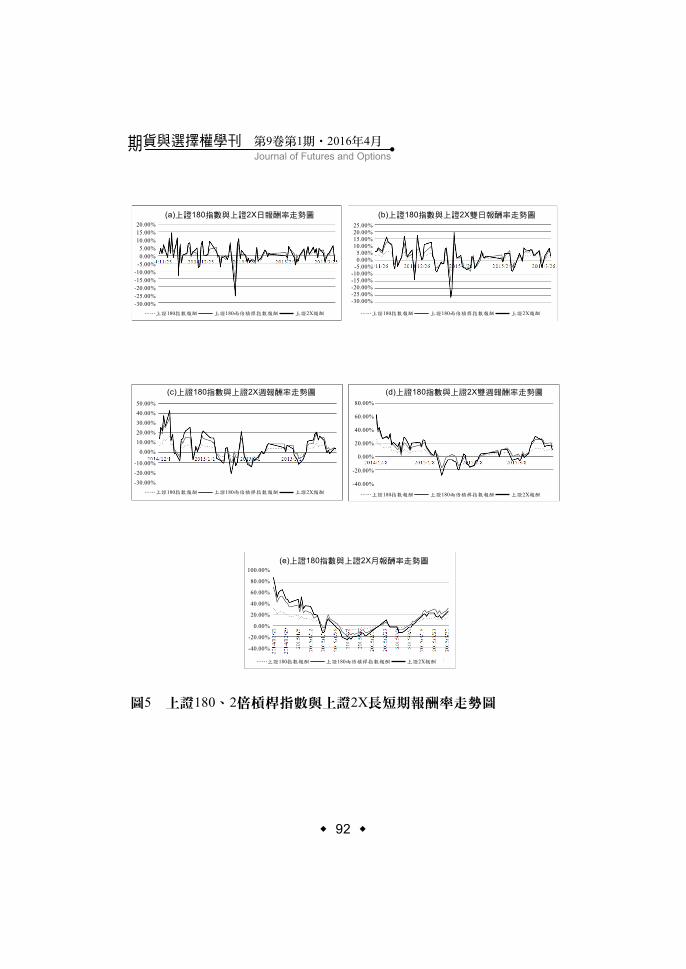
92
Journal of Futures and Options期貨與選擇權學刊 第9卷第1期 201‧ 6年4月
‧
圖5 上證180、2倍槓桿指數與上證2X長短期報酬率走勢圖
(a)上證180指數與上證2X日報酬率走勢圖 (b)上證180指數與上證2X雙日報酬率走勢圖
(c)上證180指數與上證2X週報酬率走勢圖 (d)上證180指數與上證2X雙週報酬率走勢圖
(e)上證180指數與上證2X月報酬率走勢圖
……上證180指數報酬 上證180兩倍槓桿指數報酬 上證2X報酬 ……上證180指數報酬 上證180兩倍槓桿指數報酬 上證2X報酬
……上證180指數報酬 上證180兩倍槓桿指數報酬 上證2X報酬 ……上證180指數報酬 上證180兩倍槓桿指數報酬 上證2X報酬
……上證180指數報酬 上證180兩倍槓桿指數報酬 上證2X報酬
100.00%
80.00%
60.00%
40.00%
20.00%
0.00%
-20.00%
-40.00%
80.00%
60.00%
40.00%
20.00%
0.00%
-20.00%
-40.00%
50.00%40.00%30.00%20.00%10.00%
0.00%
-10.00%-20.00%-30.00%
20.00%15.00%10.00%
5.00%0.00%
-5.00%-10.00%-15.00%-20.00%-25.00%-30.00%
25.00%20.00%15.00%10.00%
5.00%0.00%
-5.00%-10.00%-15.00%-20.00%-25.00%-30.00%
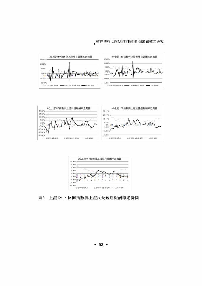
槓桿型與反向型ETF長短期追蹤績效之研究
93
‧
圖6 上證180、反向指數與上證反長短期報酬率走勢圖
(a)上證180指數與上證反日報酬率走勢圖 (b)上證180指數與上證反雙日報酬率走勢圖
(c)上證180指數與上證反週報酬率走勢圖 (d)上證180指數與上證反雙週報酬率走勢圖
(e)上證180指數與上證反月報酬率走勢圖
……上證180指數報酬 上證180反向指數報酬 上證反報酬 ……上證180指數報酬 上證180反向指數報酬 上證反報酬
……上證180指數報酬 上證180反向指數報酬 上證反報酬 ……上證180指數報酬 上證180反向指數報酬 上證反報酬
……上證180指數報酬 上證180反向指數報酬 上證反報酬
40.00%
30.00%
20.00%
10.00%
0.00%
-10.00%
-20.00%
-30.00%
-40.00%
20.00%
15.00%
10.00%
5.00%
0.00%
-5.00%
-10.00%
-15.00%
-20.00%
15.00%
10.00%
5.00%
0.00%
30.00%
20.00%
10.00%
0.00%
-10.00%
-20.00%
-30.00%
-5.00%
-10.00%
-15.00%
-5.00%
-10.00%
15.00%
10.00%
5.00%
0.00%
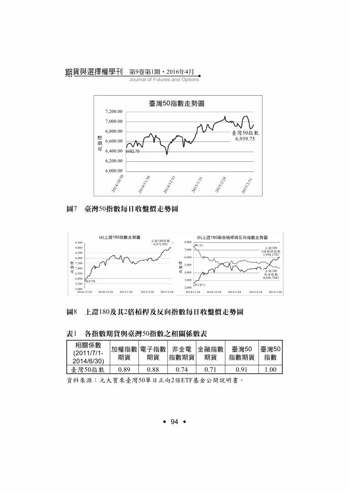
94
Journal of Futures and Options期貨與選擇權學刊 第9卷第1期 201‧ 6年4月
‧
圖7 臺灣50指數每日收盤價走勢圖
圖8 上證180及其2倍槓桿及反向指數每日收盤價走勢圖
表1 各指數期貨與臺灣50指數之相關係數表 相關係數
(2011/7/1-2014/6/30)
加權指數
期貨 電子指數
期貨 非金電
指數期貨
金融指數
期貨 臺灣50 指數期貨
臺灣50 指數
臺灣50指數 0.89 0.88 0.74 0.71 0.91 1.00 資料來源:元大寶來臺灣50單日正向2倍ETF基金公開說明書。
臺灣50指數走勢圖收
盤價
7,200.00
7,000.00
6,800.00
6,600.00
6,400.00
6,200.00
6,000.00
(a)上證180指數走勢圖 (b)上證180兩倍槓桿與反向指數走勢圖
收盤
價
收盤
價
2014/11/24 2014/12/24 2015/1/24 2015/2/24 2015/3/24 2014/11/24 2014/12/24 2015/1/24 2015/2/24 2015/3/24
9,500
9,000
8,500
8,000
7,500
7,000
6,500
6,000
5,500
5,000
8,000
7,000
6,000
5,000
4,000
3,000
2,000
2014
/10/
30
2014
/11/
30
2014
/12/
31
2015
/1/3
1
2015
/2/2
8
2015
/3/3
1
臺灣50指數 6,939.75
上證180指數8,972.903
上證180 2倍槓桿指數
5,994.2785
上證180 反向指數
4,696.7942
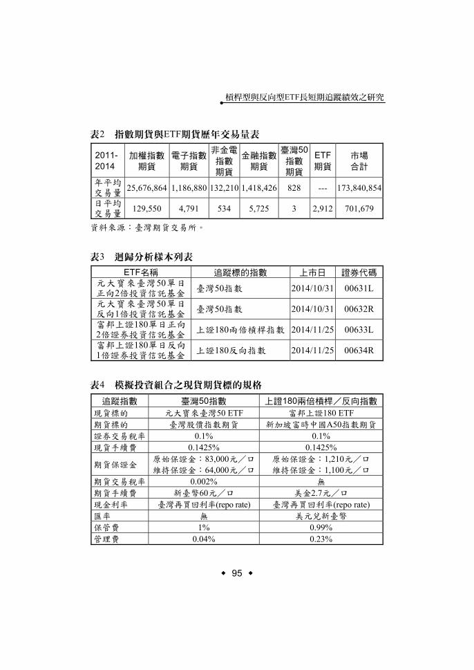
槓桿型與反向型ETF長短期追蹤績效之研究
95
‧
表2 指數期貨與ETF期貨歷年交易量表
2011- 2014
加權指數
期貨 電子指數
期貨
非金電
指數
期貨
金融指數
期貨
臺灣50指數
期貨
ETF期貨
市場 合計
年平均 交易量 25,676,864 1,186,880 132,210 1,418,426 828 --- 173,840,854
日平均 交易量 129,550 4,791 534 5,725 3 2,912 701,679
資料來源:臺灣期貨交易所。
表3 迴歸分析樣本列表
表4 模擬投資組合之現貨期貨標的規格
追蹤指數 臺灣50指數 上證180兩倍槓桿/反向指數 現貨標的 元大寶來臺灣50 ETF 富邦上證180 ETF 期貨標的 臺灣股價指數期貨 新加坡富時中國A50指數期貨 證券交易稅率 0.1% 0.1% 現貨手續費 0.1425% 0.1425%
期貨保證金 原始保證金:83,000元/口
維持保證金:64,000元/口
原始保證金:1,210元/口 維持保證金:1,100元/口
期貨交易稅率 0.002% 無 期貨手續費 新臺幣60元/口 美金2.7元/口 現金利率 臺灣再買回利率(repo rate) 臺灣再買回利率(repo rate) 匯率 無 美元兌新臺幣 保管費 1% 0.99% 管理費 0.04% 0.23%
ETF名稱 追蹤標的指數 上市日 證券代碼 元大寶來臺灣50單日正向2倍投資信託基金
臺灣50指數 2014/10/31 00631L
元大寶來臺灣50單日反向1倍投資信託基金
臺灣50指數 2014/10/31 00632R
富邦上證180單日正向2倍證券投資信託基金
上證180兩倍槓桿指數 2014/11/25 00633L
富邦上證180單日反向1倍證券投資信託基金
上證180反向指數 2014/11/25 00634R
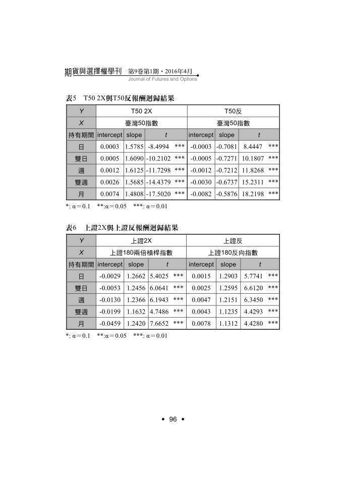
96
Journal of Futures and Options期貨與選擇權學刊 第9卷第1期 201‧ 6年4月
‧
表5 T50 2X與T50反報酬迴歸結果 Y T50 2X T50反
X 臺灣50指數 臺灣50指數
持有期間 intercept slope t intercept slope t
日 0.0003 1.5785 -8.4994 *** -0.0003 -0.7081 8.4447 ***
雙日 0.0005 1.6090 -10.2102 *** -0.0005 -0.7271 10.1807 ***
週 0.0012 1.6125 -11.7298 *** -0.0012 -0.7212 11.8268 ***
雙週 0.0026 1.5685 -14.4379 *** -0.0030 -0.6737 15.2311 ***
月 0.0074 1.4808 -17.5020 *** -0.0082 -0.5876 18.2198 ***
*: α=0.1 **:α=0.05 ***: α=0.01
表6 上證2X與上證反報酬迴歸結果
Y 上證2X 上證反
X 上證180兩倍槓桿指數 上證180反向指數
持有期間 intercept slope t intercept slope t
日 -0.0029 1.2662 5.4025 *** 0.0015 1.2903 5.7741 ***
雙日 -0.0053 1.2456 6.0641 *** 0.0025 1.2595 6.6120 ***
週 -0.0130 1.2366 6.1943 *** 0.0047 1.2151 6.3450 ***
雙週 -0.0199 1.1632 4.7486 *** 0.0043 1.1235 4.4293 ***
月 -0.0459 1.2420 7.6652 *** 0.0078 1.1312 4.4280 ***
*: α=0.1 **:α=0.05 ***: α=0.01
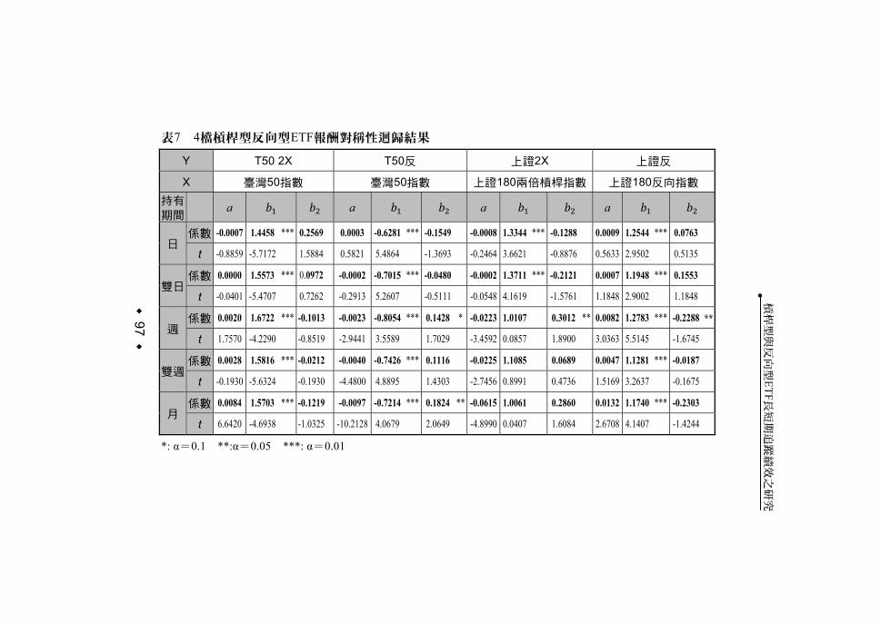
表7 4檔槓桿型反向型ETF報酬對稱性迴歸結果 Y T50 2X T50反 上證2X 上證反
X 臺灣50指數 臺灣50指數 上證180兩倍槓桿指數 上證180反向指數 持有 期間 a a a a
日 係數 -0.0007 1.4458 *** 0.2569 0.0003 -0.6281 *** -0.1549 -0.0008 1.3344 *** -0.1288 0.0009 1.2544 *** 0.0763
t -0.8859 -5.7172 1.5884 0.5821 5.4864 -1.3693 -0.2464 3.6621 -0.8876 0.5633 2.9502 0.5135
雙日 係數 0.0000 1.5573 *** 0.0972 -0.0002 -0.7015 *** -0.0480 -0.0002 1.3711 *** -0.2121 0.0007 1.1948 *** 0.1553
t -0.0401 -5.4707 0.7262 -0.2913 5.2607 -0.5111 -0.0548 4.1619 -1.5761 1.1848 2.9002 1.1848
週 係數 0.0020 1.6722 *** -0.1013 -0.0023 -0.8054 *** 0.1428 * -0.0223 1.0107 0.3012 ** 0.0082 1.2783 *** -0.2288 **
t 1.7570 -4.2290 -0.8519 -2.9441 3.5589 1.7029 -3.4592 0.0857 1.8900 3.0363 5.5145 -1.6745
雙週 係數 0.0028 1.5816 *** -0.0212 -0.0040 -0.7426 *** 0.1116 -0.0225 1.1085 0.0689 0.0047 1.1281 *** -0.0187
t -0.1930 -5.6324 -0.1930 -4.4800 4.8895 1.4303 -2.7456 0.8991 0.4736 1.5169 3.2637 -0.1675
月 係數 0.0084 1.5703 *** -0.1219 -0.0097 -0.7214 *** 0.1824 ** -0.0615 1.0061 0.2860 0.0132 1.1740 *** -0.2303
t 6.6420 -4.6938 -1.0325 -10.2128 4.0679 2.0649 -4.8990 0.0407 1.6084 2.6708 4.1407 -1.4244
*: α=0.1 **:α=0.05 ***: α=0.01
槓桿
型與
反向
型ETF
長短
期追
蹤績
效之
研究
97
‧
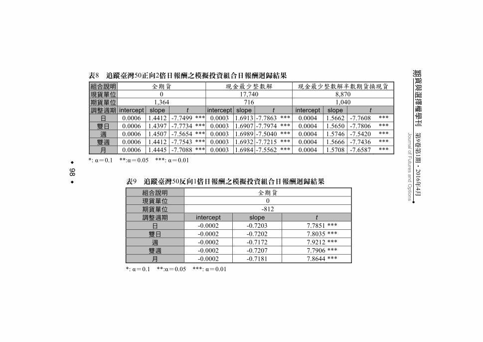
表8 追蹤臺灣50正向2倍日報酬之模擬投資組合日報酬迴歸結果 組合說明 全期貨 現金最少整數解 現金最少整數解半數期貨換現貨現貨單位 0 17,740 8,870 期貨單位 1,364 716 1,040 調整週期 intercept slope t intercept slope t intercept slope t
日 0.0006 1.4412 -7.7499 *** 0.0003 1.6913 -7.7863 *** 0.0004 1.5662 -7.7608 ***雙日 0.0006 1.4397 -7.7734 *** 0.0003 1.6907 -7.7974 *** 0.0004 1.5650 -7.7806 ***週 0.0006 1.4507 -7.5654 *** 0.0003 1.6989 -7.5040 *** 0.0004 1.5746 -7.5420 ***
雙週 0.0006 1.4412 -7.7543 *** 0.0003 1.6932 -7.7215 *** 0.0004 1.5666 -7.7436 ***月 0.0006 1.4445 -7.7088 *** 0.0003 1.6984 -7.5562 *** 0.0004 1.5708 -7.6587 ***
*: α=0.1 **:α=0.05 ***: α=0.01
表9 追蹤臺灣50反向1倍日報酬之模擬投資組合日報酬迴歸結果
組合說明 全期貨 現貨單位 0 期貨單位 -812 調整週期 intercept slope t
日 -0.0002 -0.7203 7.7851 *** 雙日 -0.0002 -0.7202 7.8035 *** 週 -0.0002 -0.7172 7.9212 ***
雙週 -0.0002 -0.7207 7.7906 *** 月 -0.0002 -0.7181 7.8644 *** *: α=0.1 **:α=0.05 ***: α=0.01
98
期貨
與選
擇權
學刊
第
9卷
第1期
201‧
6年
4月
Journal of Futures and O
ptions
‧
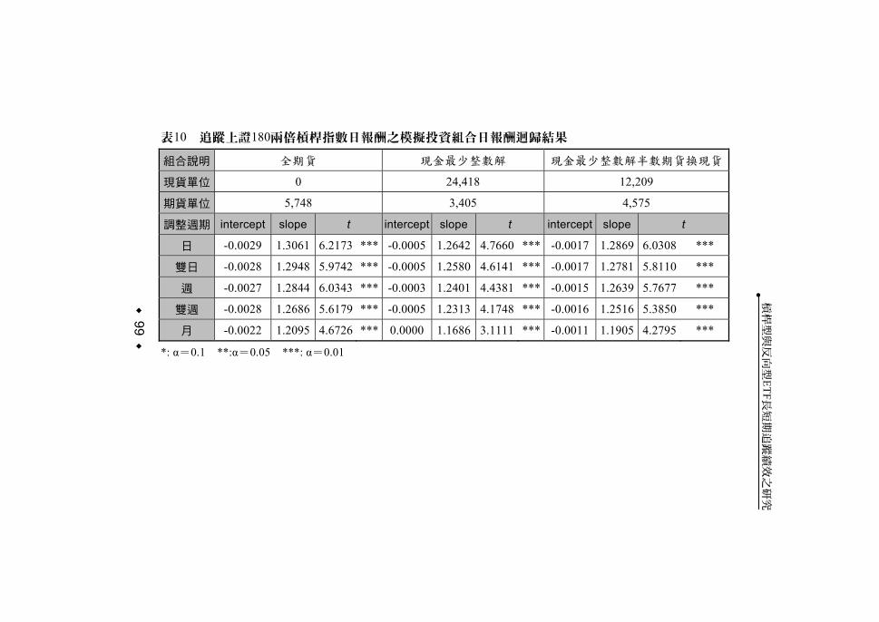
表10 追蹤上證180兩倍槓桿指數日報酬之模擬投資組合日報酬迴歸結果 組合說明 全期貨 現金最少整數解 現金最少整數解半數期貨換現貨
現貨單位 0 24,418 12,209
期貨單位 5,748 3,405 4,575
調整週期 intercept slope t intercept slope t intercept slope t
日 -0.0029 1.3061 6.2173 *** -0.0005 1.2642 4.7660 *** -0.0017 1.2869 6.0308 ***
雙日 -0.0028 1.2948 5.9742 *** -0.0005 1.2580 4.6141 *** -0.0017 1.2781 5.8110 ***
週 -0.0027 1.2844 6.0343 *** -0.0003 1.2401 4.4381 *** -0.0015 1.2639 5.7677 ***
雙週 -0.0028 1.2686 5.6179 *** -0.0005 1.2313 4.1748 *** -0.0016 1.2516 5.3850 ***
月 -0.0022 1.2095 4.6726 *** 0.0000 1.1686 3.1111 *** -0.0011 1.1905 4.2795 ***
*: α=0.1 **:α=0.05 ***: α=0.01
槓桿
型與
反向
型ETF
長短
期追
蹤績
效之
研究
99
‧
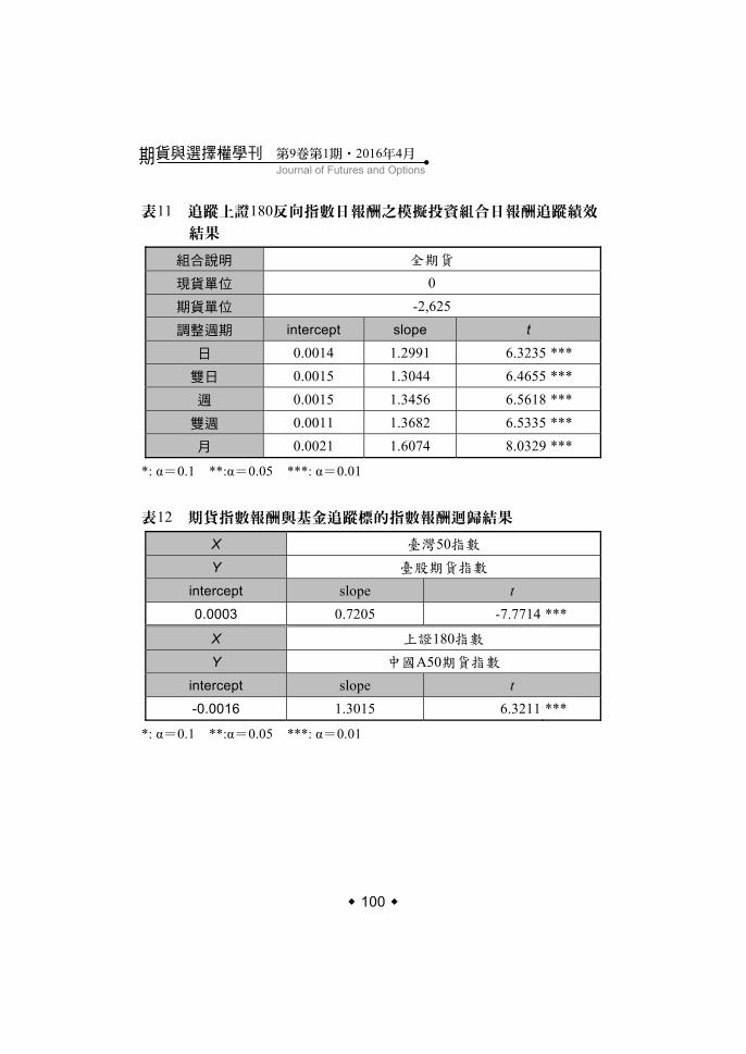
100
Journal of Futures and Options期貨與選擇權學刊 第9卷第1期‧2016年4月
‧
表11 追蹤上證180反向指數日報酬之模擬投資組合日報酬追蹤績效
結果 組合說明 全期貨 現貨單位 0 期貨單位 -2,625 調整週期 intercept slope t
日 0.0014 1.2991 6.3235 *** 雙日 0.0015 1.3044 6.4655 *** 週 0.0015 1.3456 6.5618 ***
雙週 0.0011 1.3682 6.5335 *** 月 0.0021 1.6074 8.0329 ***
*: α=0.1 **:α=0.05 ***: α=0.01
表12 期貨指數報酬與基金追蹤標的指數報酬迴歸結果
X 臺灣50指數 Y 臺股期貨指數
intercept slope t 0.0003 0.7205 -7.7714 ***
X 上證180指數 Y 中國A50期貨指數
intercept slope t -0.0016 1.3015 6.3211 ***
*: α=0.1 **:α=0.05 ***: α=0.01
槓桿型與反向型ETF長短期追蹤績效之研究
101
‧
參考文獻
Avellaneda, Marco and Stanley Zhang (2010), “Path-Dependence of Leveraged ETF Returns,” SIAM Journal on Financial Mathematics, 1(1), 586-603. Cheng, Minder and Ananth Madhavan (2009), “The Dynamics of Leveraged and Inverse Exchange-Traded Funds,” Journal of Investment Management (JOIM), Fourth Quarter. Jarrow, Robert A. (2010), “Understanding the Risk of Leveraged ETFs,” Finance Research Letters, 7(3), 135-139. Little, Patricia Knain (2010), “Inversed and Leveraged ETFs: Not Your Father’s ETF,” Journal of Index Investing, 1(1), 83-89. Lu, Lei, Jun Wang and Ge Zhang (2009), “Long Term Performance of Leveraged ETFs,” Available at SSRN, 1344133. Trainor Jr., William J. and Mark G. Carroll (2013), “Forecasting Holding Periods for Leveraged ETFs Using Decay Thresholds: Theory and Applications,” Journal of Financial Studies & Research 2013, 1-12. Trainor Jr., William J. (2010), “Do Leveraged ETFs Increase Volatility,” Technology and Investment, 1(3), 215-220.

103
The Impact of Speculative Trading Activity on Return and Volatility inTaiwan Futures Market ‧
投機交易活動對臺灣期貨市場 報酬與波動的衝擊
The Impact of Speculative Trading Activity on Return and Volatility in Taiwan
Futures Market
洪瑞成* Jui-Cheng Hung
王偉權** Wei-Chuan Wang
* 通訊作者︰中國文化大學財務金融系,臺北市11114陽明山華岡路55號,
電話:+886-2-28610511轉36240;Email: [email protected]。 Department of Banking and Finance, Chinese Culture University
** 中國文化大學財務金融系。 Department of Banking and Finance, Chinese Culture University
投稿日期:2016年2月17日;第一次修訂:2016年3月15日;接受刊登日:
2016年3月21日 Received: Feb. 17, 2016; First Revision: Mar. 15, 2016; Accepted: Mar. 21, 2016

104
Journal of Futures and Options期貨與選擇權學刊 第9卷第1期 201‧ 6年4月
‧
Contents
I. Introduction II. Methodology
1. Variable Measurement 2. Unit Root Test 3. Vector Autoregression
Model
III. Empirical Results ◎ Data Description and
Preliminary Analysis IV. Conclusion

105
The Impact of Speculative Trading Activity on Return and Volatility inTaiwan Futures Market ‧
摘 要
本研究探討投機性交易活動對臺灣期貨市場報酬率與波動
的衝擊。過去研究通常使用交易量或是未平倉量衡量交易活
動。然而,此兩變數無法捕捉期貨市場中的投機性交易活動。
本研究使用Garcia et al. (1986)提出的交易量除以未平倉量之比率
作為另一衡量投機性交易活動用以探討不同交易人之投機性交
易活動和報酬與波動之關係。實證研究顯示國外機構投資人為
反向交易者;相反的,個別交易人為動能交易者。根據避險壓
力效果和市場擇時能力,本研究認為國外機構投資人和個別交
易人在臺灣期貨市場中分別為投機者與避險者。
關鍵詞:交易人種類、反向交易者、動能交易者、避險者、投
機者
106
Journal of Futures and Options期貨與選擇權學刊 第9卷第1期 201‧ 6年4月
‧
Abstract
The study examines the impact of speculative trading activity on return and volatility in Taiwan futures market. Previous studies generally use trading volume or open interest to measure trading activities. However, these two variables are failed to seize the speculative trading activities in futures market. This study uses the ratio of trading volume over open interest suggested by Garcia et al. (1986) as an alternative manner to examine the relationship among return, volatility and (speculative) trading activity of trader type. Empirical results show that the foreign institutional investors are contrarian traders; on the contrary, retail investors are momentum traders. According to hedging pressure effects and market timing ability, this study concludes that foreign institutional investors are speculators and retail investors are hedgers in Taiwan futures market.
Keywords: Trader Type, Contrarian, Momentum, Hedgers, Speculators
107
The Impact of Speculative Trading Activity on Return and Volatility inTaiwan Futures Market ‧
I. Introduction
The trading behavior of institutional and retail (individual) investors in financial markets is always a popular issue for financial researchers and regulators. In recent years, the access of transaction-level data enables academic researchers and practitioners to analyse this issue and establish trading strategy in a more detailed way. Previous findings show that the performance of stock (index) price might depend on how institutional and retail investors trade, and the trading behaviors of institutional and retail investors are systematically diverse when facing dynamics of past price, and follow momentum (positive feedback) or contrarian (negative feedback) strategies.
Taiwan stock market plays an importance role around the worldwide stock markets because many heavy-weighted IT companies attracts numerous foreign institutional investors to put money into this market. In view of its importance around the world, research topics related to operation and functionality of its derivative market are no doubt very fascinating and momentous to academics and practitioners.1 Lee et al. (1999) used a vector autoregressive model to examine interactive relationship among institutional investors, big and small individual investors, and the impacts of their trading on stock returns in Taiwan stock market. During their research period, the results suggested that big individual investors are the major informed
1 Based on the latest report of Taiwan futures exchange (TAIFEX) in May
2014, their trading volume is ranked in 21th among the world derivative exchanges. For the financial index futures exchanges among Asian countries, TAIFEX is ranked in 6th.
108
Journal of Futures and Options期貨與選擇權學刊 第9卷第1期 201‧ 6年4月
‧
traders; their trading influence both stock returns and the behavior of small individual investors. Moreover, institional investors do not engage in momentum or contrarian strategies. Chiang et al. (2012) used a threshold cointegration model of Hansen and Seo (2002) to examine the nonlinear behavior of three trader types across regimes in Taiwan stock market. They found that none of three trader types showed predominance in stock market. The direction of trading positions for individual investors was positively related to stock prices when the market was close to equilibrium. However, when the market was substantially deviated from equilibrium, the trading directions of both institutional investors were positively related to stock prices. In contrast, individual investors tended to lose during this regime.
Wang (2003) examined the behavior and performance of speculators and hedgers in 15 U.S. futures markets. They found that speculators are contrarian traders, and in contrast, hedgers are momentum traders. Moreover, trades of speculators (hedger) are correlated with subsequent abnormal returns; however, it does not indicate that speculators possess superior forecasting power. The positive feedback trading by hedgers together with their negative performance suggests that hedgers have a destabilizing impact on futures prices. Cheng et al. (2007) investigated the trading behavior and performance of four trader types in Taiwan futures market during 2001 to 2002. They found that foreign institutional investors are negative feedback (contrarian) traders; in contrast, domestic investors, including proprietary and retail investors, are positive feedback (momentum) traders. In addition, foreign institutional and retail investors are main profitors and losers respectively in Taiwan futures
109
The Impact of Speculative Trading Activity on Return and Volatility inTaiwan Futures Market ‧
market during this period. In sum, the majority of previous studies, which examines trading behaviors of trader type in stock market, finds that institutional investors tend to be momentum traders and retail investors are contrarian traders. Kurov (2008) used transaction data of two actively traded index futures (S&P 500 and Nasdaq 100 E-mini) in CME (Chicago Mercentile Exchange) to investigate whether investors are positive or negative feedback traders. The results showed that index futures investors engage in positive feedback trading, and the positive feedback trading intensifies during high investor sentiment period.
While the existing results offer important insights into the trading behaviors of institutional and retail investors, they focus mainly on equity markets, and relatively little is known about the behavior and performance of traders in futures markets. This study examines the relationsip among return, volatility and trading activity of trader type in Taiwan futures market. Without the trading information like the CFTC’s (Commidity Futures Trading Commission) COT 2
(Commitments of Traders) reports, previous studies commonly use trading volume and open interest to measure speculative and hedging trading activities respectively. However, these two variables are failed
2 The COT reports contain reportable and nonreportable ones. The repotable
positions are classified as commercial and noncommercial. Traders with commercial positions to hedge specific risks are regarded as hedgers; in contrast, traders with noncommercial positions are speculators. Traders with small positions which are nonreportable are small traders. Various studies (Wang, 2003, 2004; Sanders et al., 2004; Röthig and Chiarella, 2007; Chatrath et al., 2010; Chang et al., 2013) uses the COT reports to measure the trading activity with different purposes in futures markets.
110
Journal of Futures and Options期貨與選擇權學刊 第9卷第1期 201‧ 6年4月
‧
to seize the speculative trading activity in futures market. This study uses the ratio of trading volume over open interest, as suggested by Garcia et al. (1986), to examine the relationship among return, volatility and (speculative) trading activity of trader type. The primary research goal of this study is twofold. First, we investigate the relationship between returns, volatilities and trading activity by trader type. The trading activity is proxied by the net buy trading volume, which is defined by using buy trading volume minus sell trading volume. Second, the trading purposes of trader type are hard to be distinguished from simply using trading volume because it comprises of speculative, hedging and liquidity demands. In order to differentiate trading purposes from trading information, we defined the ratio of net buy trading volume over open interest to proxy speculative trading activity of trader type and further examine the relationship between returns, volatilities and speculative trading activity. It is expected that the usage of two kinds of trading activity measures would provide regulators and traders with important insights into the interactions among the relationship of return, volatility and trading activity of trader type in Taiwan futures market.
Based on previous arguments by Llorente et al. (2002) and Merton (1973, 1987), if an investor trades for hedging purposes, asset prices must decrease (increase) to attract speculators to buy (sell). Thus, the testing hypothesis can be established that the (speculative) trading activity would be granger-caused by past return. This imples that the speculative trading activity would be granger-caused by past return. The empirical results show that there are some discrepancies when trading volume and trading volume over open interest are used
111
The Impact of Speculative Trading Activity on Return and Volatility inTaiwan Futures Market ‧
as the proxy of trading activity. Irrespective of trading activity proxy, the foreign institutional investors are contrarian traders and retail investors are momentum traders. For domestic institutional investors, they engage in contrarian trading when using net buy volume over open interest to proxy their trading activity, but there is no significant evidence when using the other proxy. Our findings are consistent with Wang (2003), which suggests that speculators are contrarian traders. In addition, the results of net buy volume indicate that foreign institutional investors tend to make profit and retail investors tend lose money. However, no significant evidence shows that speculative trading activities of foreign institutional and retail investors make or lose money. As for the impacts of trading activity on volatility, only speculative trading of domestic institutional investors destabilizes the futures market.
The remainder of this paper is organized as follows: Section 2 introduces the econometric methodology, including the variable measurement, unit root test and vector autoregressive model. Section 3 reports the main findings and Section 4 offers concluding remarks.
II. Methodology
1. Variable Measurement The close-to-close return is used to compute daily index futures
return. Because the close-to-close return contains overnight return, the one-minute realized variance computed in this study also comprises overnight variance. The computation manners for return and realized variance (RV) are represented as follows:
112
Journal of Futures and Options期貨與選擇權學刊 第9卷第1期 201‧ 6年4月
‧
1100 c ct t tR ln( P P )−= × (1)
21
2
1 11100 100
Mt t ,ii
2M c c o ct ,i t ,i t ti
RV R overnight variance
ln( P P ) ln( P P )
=
− −=
= +
⎡ ⎤ ⎡ ⎤= × + ×⎣ ⎦ ⎣ ⎦
∑∑
(2)
where, ctP and o
tP denote daily closing and opening price of index futures, respectively. c
t ,iP denotes the closing price of the i-th intraday
interval at day t. The regular trading hour in Taiwan futures exchange (TAIFEX) begins at 8:45 a.m. and ends at 1:45 p.m.. Thus, each trading day amounts to a duration of 300M ×∆ = mins. For =∆ 1 min, we have M = 300 intraday returns.3
Prevoius studies extensively used trading volume or open interest (OI) to measure trading activity and examined its variablility with return, volatility and other related variables in the futures market (Bessembinder and Seguin (1992, 1993); Huang, 2002; Wang and Yu, 2004; Kuo, Hsu and Chiang, 2005). Because most speculators tend to be day traders who worry about overnight risk of holding open positions, open interest primarily reflects hedging activity and, thus, can be considered as the amount of uninformed trading (Bessembinder
3 The sampling frequency of one minute is used as a compromise between
sampling error of the estimates and the microstructure bias (Andersen et al., 2001; Fleming et al., 2003; Koopman et al., 2005). We also use five minutes frequency to compute RV and the results are similar to those with one minute. Moreover, the Parkinson (1980) extreme-value estimator is used as a robustness check. Once again, the results are similar to those with RV. Thus, these additional works are not reported in this study and are available upon request.
113
The Impact of Speculative Trading Activity on Return and Volatility inTaiwan Futures Market ‧
and Seguin, 1993). Unlike CFTC’s COT reports, TAIFEX does not release this kind of trading information. For this reason, it’s hard to directly measure speculative trading activity in Taiwan futures market.
Because neither trading volume nor open interest can precisely reflects the specific impact of speculative trading activity and seizes the information arrivals, this study uses the ratio of trading volume over open interest, as suggested by Garcia et al. (1986) and others,4 as an alternative manner to capture the dynamics of speculative trading activity in futures market. Garcia et al. (1986) argued that the main advantage of this ratio is to mitigate the possible time effect on trading activity because trading volume and open interest are both functions of time to maturity. Moreover, Luu and Martens (2003) believed that this ratio is highly capable of grabbing information arrivals than trading volume or open interest does.
TAIFEX releases all trading information of both trading volume and open interest for three main institutional traders (including foreign institutional, investment trust companies, and proprietary traders) after 3:00 p.m. on daily basis since July 2, 2007. Trading volume and open interest are summed across the nearest and second nearest contracts to obtain an aggregate measure of activity for the stock index futures in TAIFEX. The net buy trading volume (NBVOL) and net buy volume over open interest (NBVOI) for trader type i on day t are given by:
i i it t tNBVOL ln( buy volume ) - ln(sell volume )= (3)
4 This measurement of speculative trading activity is also employed by
Chatrath et al. (1995, 1996), Kyriacou and Sarno (1999), Hagelin (2000), and Luu and Martens (2003).
114
Journal of Futures and Options期貨與選擇權學刊 第9卷第1期 201‧ 6年4月
‧
i ii t tt i i
t t
buy volume sell volumeNBVOI ( ) - ( ) for i=FT, DT, RTbuy OI sell OI
= (4)
where, FT, DT, and RT denotes foreign institutional, domestic institutional and retail traders. Domestic institutional trader comprises investment trust companies and proprietary traders. The buy and sell volume and open interest for retail trader can be computed by using trading volume and open interest of whole market to deduct those of three main institutional traders.
2. Unit Root Test The vector autoregression (VAR) model used in this study for
casuality test assumes that the variables in the system are stationary. For this reason, we test for the stationarity of all variables, including return, realized volatility and trading activity of trader types. Previous studies (Gallant et al., 1992) indicate that there might be linear or nonlinear time trend in trading activity proxied by trading volumes. Thus, we adopt augmented Dickey and Fuller (ADF) test (1979) with two versions of linear time trend and nonlinear time trend to proceed unit-root test for all variables. The ADF regression is expressed as follows:
20 1 2 1
pt t i t i ti
y t t y y −=∆ = α +α +α + γ + β + ε∑ (5)
where, the null hypothesis for testing a unit root is 0 0H : γ = .
Rejecting null hypothesis implies that a series is stationary.
3. Vector Autoregression Model The relationship among return, volatility and trading acivity has
115
The Impact of Speculative Trading Activity on Return and Volatility inTaiwan Futures Market ‧
been extensively studied by presvious researches for different assets and markets. This study examines the granger-casality relationship by the use of a vector autoregressive (VAR) system for return, volatility and trading activity of stock index futures in Taiwan futures market. Moreover, the impulse response function in the VAR system allows this study to further comprehend how an impact of one variable in the system influences the conditional forecast of the other variable. The VAR model used in this study is expressed as follows:
20 1 2 3 1
1 1 1
p p p
t i t i i t i i t i ti i i
R R TA− − −= = =
= α + α + α σ + α + ε∑ ∑ ∑ (6)
2 20 1 2 3 2
1 1 1
p p p
t i t i i t i i t i ti i i
R TA− − −= = =
σ = β + β + β σ + β + ε∑ ∑ ∑ (7)
20 1 2 3 3
1 1 1
p p p
t i t i i t i i t i ti i i
TA R TA− − −= = =
= γ + γ + γ σ + γ + ε∑ ∑ ∑ (8)
where, 1 2 3i i i, , α β γ are the parameters of lagged regressors and
2 3 1 3 1 3i i i i i i, , , , , α α β β γ γ are parameters of lagged independent variables. 1 2 3t t t, , ε ε ε denote error term in each equations. TAt stands
for trading activity, i.e. NBVOL or NBVOI. Optimal lag length for the VAR model is determined by Schwartz Bayesian Criterion (SBC) according to the parisomonious principle. ADF test is used to confirm the stationarity of all varibles as VAR is appropriate model if, and only if, the series are stationary.
When the estimation of VAR model is done, the Granger causality testcan be proceeded by running regressions in Eqs. (6)~(8) with and without the lagged independent variables and computing the
116
Journal of Futures and Options期貨與選擇權學刊 第9卷第1期 201‧ 6年4月
‧
F-statistics. For example, to test whether volatility granger-causes return by using Eq. (6) , the null hypothese is given by
0 21 22 2pH : 0α = α = = α = . If H0 is true, the F-test statistic is given by:
3 13 1
R U
U
( RSS RSS ) pF ~ F( p,T p )RSS (T p )
−= − −− −
(9)
where, RSSR and RSSF denote the restricted and unrestricted residual sum of squares respectively. T is the number of observations. If H0 is significantly rejected, it indicates that past volatility has an explanation ability to the return now.
III. Empirical Results
◎ Data Description and Preliminary Analysis The data used in the empirical section including the daily prices
(opening, high, low, closing price), trading volume and open interest of the nearest and second nearest futures contracts for the stock index futures in Taiwan futures exchange (TAIFEX). One-minute closing prices during the regular trading hour from 8:45 a.m. to 1:45 p.m. are used to compute realized volatility (RV). The TAIFEX discloses all trading information of both trading volume and open interest for three main institutional traders (including foreign institutional, investment trust companies, and proprietary traders) every day. The data used in this study are all retrieved from the Taiwan Economic Journal (TEJ), and the research period is from January 6, 2009, to December 31,
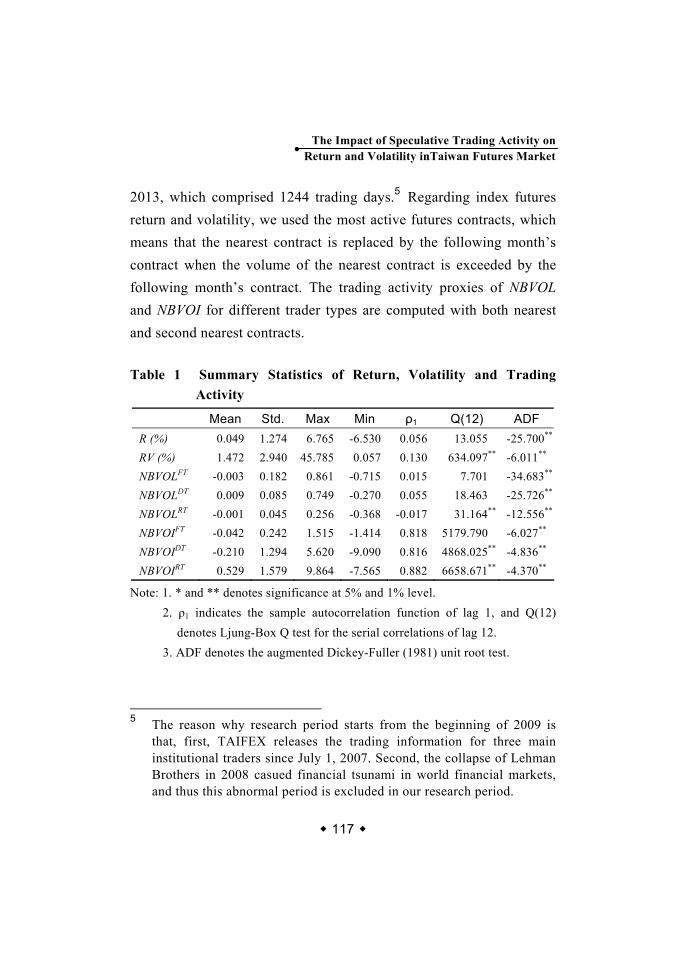
117
The Impact of Speculative Trading Activity on Return and Volatility inTaiwan Futures Market ‧
2013, which comprised 1244 trading days.5 Regarding index futures return and volatility, we used the most active futures contracts, which means that the nearest contract is replaced by the following month’s contract when the volume of the nearest contract is exceeded by the following month’s contract. The trading activity proxies of NBVOL and NBVOI for different trader types are computed with both nearest and second nearest contracts.
Table 1 Summary Statistics of Return, Volatility and Trading
Activity
Mean Std. Max Min ρ1 Q(12) ADF R (%) 0.049 1.274 6.765 -6.530 0.056 13.055 -25.700**
RV (%) 1.472 2.940 45.785 0.057 0.130 634.097** -6.011**
NBVOLFT -0.003 0.182 0.861 -0.715 0.015 7.701 -34.683**
NBVOLDT 0.009 0.085 0.749 -0.270 0.055 18.463 -25.726** NBVOLRT -0.001 0.045 0.256 -0.368 -0.017 31.164** -12.556** NBVOIFT -0.042 0.242 1.515 -1.414 0.818 5179.790 -6.027** NBVOIDT -0.210 1.294 5.620 -9.090 0.816 4868.025** -4.836** NBVOIRT 0.529 1.579 9.864 -7.565 0.882 6658.671** -4.370**
Note: 1. * and ** denotes significance at 5% and 1% level. 2. ρ1 indicates the sample autocorrelation function of lag 1, and Q(12)
denotes Ljung-Box Q test for the serial correlations of lag 12. 3. ADF denotes the augmented Dickey-Fuller (1981) unit root test.
5 The reason why research period starts from the beginning of 2009 is
that, first, TAIFEX releases the trading information for three main institutional traders since July 1, 2007. Second, the collapse of Lehman Brothers in 2008 casued financial tsunami in world financial markets, and thus this abnormal period is excluded in our research period.
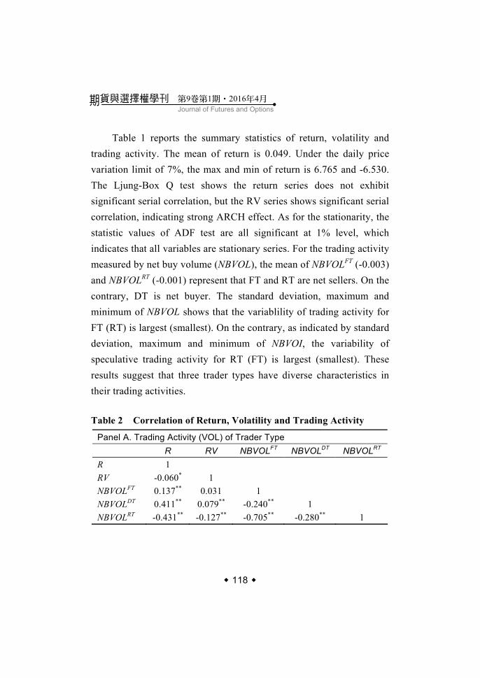
118
Journal of Futures and Options期貨與選擇權學刊 第9卷第1期 201‧ 6年4月
‧
Table 1 reports the summary statistics of return, volatility and trading activity. The mean of return is 0.049. Under the daily price variation limit of 7%, the max and min of return is 6.765 and -6.530. The Ljung-Box Q test shows the return series does not exhibit significant serial correlation, but the RV series shows significant serial correlation, indicating strong ARCH effect. As for the stationarity, the statistic values of ADF test are all significant at 1% level, which indicates that all variables are stationary series. For the trading activity measured by net buy volume (NBVOL), the mean of NBVOLFT (-0.003) and NBVOLRT (-0.001) represent that FT and RT are net sellers. On the contrary, DT is net buyer. The standard deviation, maximum and minimum of NBVOL shows that the variablility of trading activity for FT (RT) is largest (smallest). On the contrary, as indicated by standard deviation, maximum and minimum of NBVOI, the variability of speculative trading activity for RT (FT) is largest (smallest). These results suggest that three trader types have diverse characteristics in their trading activities.
Table 2 Correlation of Return, Volatility and Trading Activity
Panel A. Trading Activity (VOL) of Trader Type R RV NBVOLFT NBVOLDT NBVOLRT R 1 RV -0.060* 1 NBVOLFT 0.137** 0.031 1 NBVOLDT 0.411** 0.079** -0.240** 1 NBVOLRT -0.431** -0.127** -0.705** -0.280** 1
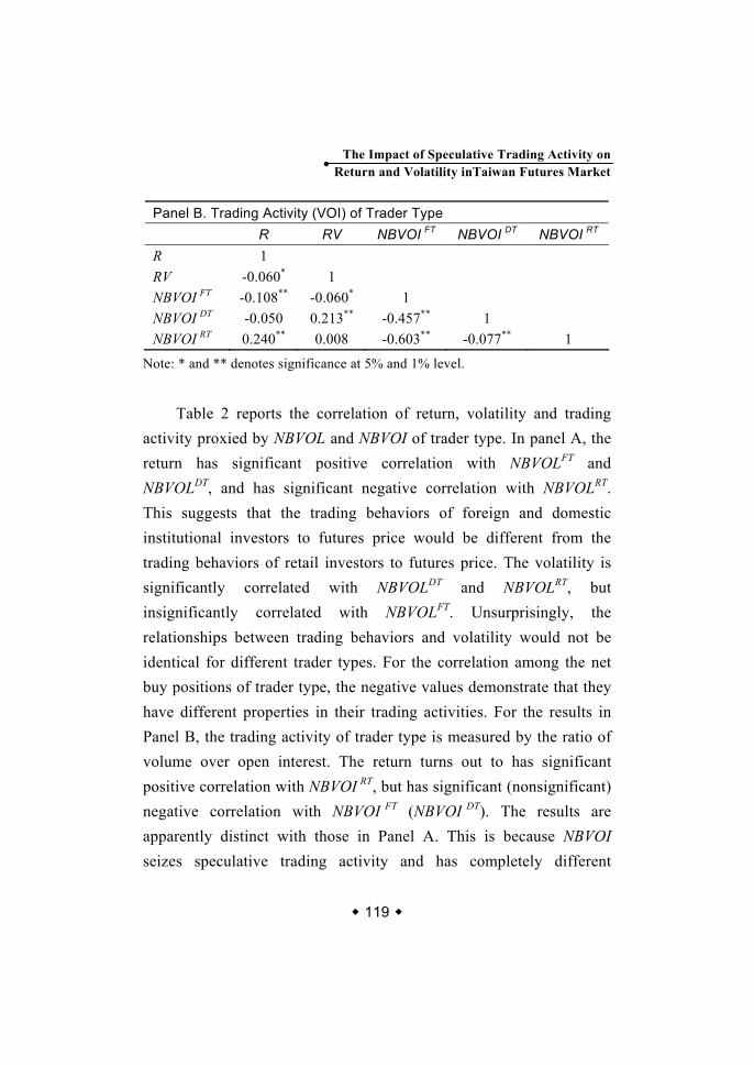
119
The Impact of Speculative Trading Activity on Return and Volatility inTaiwan Futures Market ‧
Panel B. Trading Activity (VOI) of Trader Type R RV NBVOI FT NBVOI DT NBVOI RT R 1 RV -0.060* 1 NBVOI FT -0.108** -0.060* 1 NBVOI DT -0.050 0.213** -0.457** 1 NBVOI RT 0.240** 0.008 -0.603** -0.077** 1
Note: * and ** denotes significance at 5% and 1% level.
Table 2 reports the correlation of return, volatility and trading
activity proxied by NBVOL and NBVOI of trader type. In panel A, the return has significant positive correlation with NBVOLFT and NBVOLDT, and has significant negative correlation with NBVOLRT. This suggests that the trading behaviors of foreign and domestic institutional investors to futures price would be different from the trading behaviors of retail investors to futures price. The volatility is significantly correlated with NBVOLDT and NBVOLRT, but insignificantly correlated with NBVOLFT. Unsurprisingly, the relationships between trading behaviors and volatility would not be identical for different trader types. For the correlation among the net buy positions of trader type, the negative values demonstrate that they have different properties in their trading activities. For the results in Panel B, the trading activity of trader type is measured by the ratio of volume over open interest. The return turns out to has significant positive correlation with NBVOI RT, but has significant (nonsignificant) negative correlation with NBVOI
FT (NBVOI
DT). The results are apparently distinct with those in Panel A. This is because NBVOI seizes speculative trading activity and has completely different
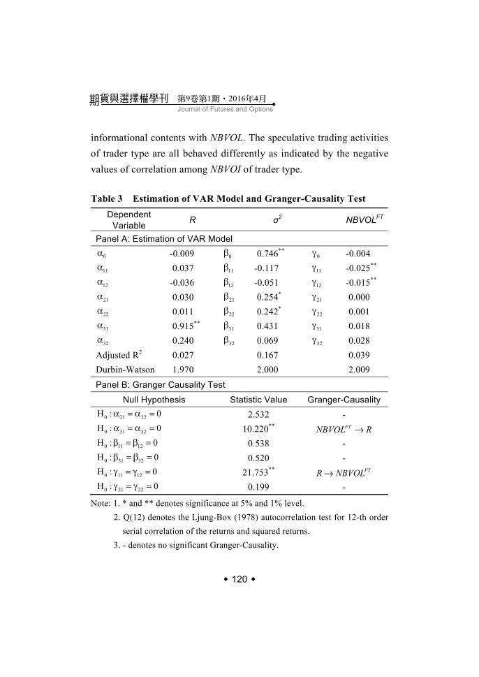
120
Journal of Futures and Options期貨與選擇權學刊 第9卷第1期 201‧ 6年4月
‧
informational contents with NBVOL. The speculative trading activities of trader type are all behaved differently as indicated by the negative values of correlation among NBVOI of trader type.
Table 3 Estimation of VAR Model and Granger-Causality Test
Dependent Variable R σ2 NBVOLFT
Panel A: Estimation of VAR Model
0α -0.009 0β 0.746** 0γ -0.004
11α 0.037 11β -0.117 11γ -0.025**
12α -0.036 12β -0.051 12γ -0.015**
21α 0.030 21β 0.254* 21γ 0.000
22α 0.011 22β 0.242* 22γ 0.001
31α 0.915** 31β 0.431 31γ 0.018
32α 0.240 32β 0.069 32γ 0.028 Adjusted R2 0.027 0.167 0.039 Durbin-Watson 1.970 2.000 2.009 Panel B: Granger Causality Test
Null Hypothesis Statistic Value Granger-Causality
0 21 22H : 0α = α = 2.532 -
0 31 32H : 0α = α = 10.220** FTNBVOL R→
0 11 12H : 0β = β = 0.538 -
0 31 32H : 0β = β = 0.520 -
0 11 12H : 0γ = γ = 21.753** FTR NBVOL→
0 21 22H : 0γ = γ = 0.199 -
Note: 1. * and ** denotes significance at 5% and 1% level. 2. Q(12) denotes the Ljung-Box (1978) autocorrelation test for 12-th order
serial correlation of the returns and squared returns. 3. - denotes no significant Granger-Causality.
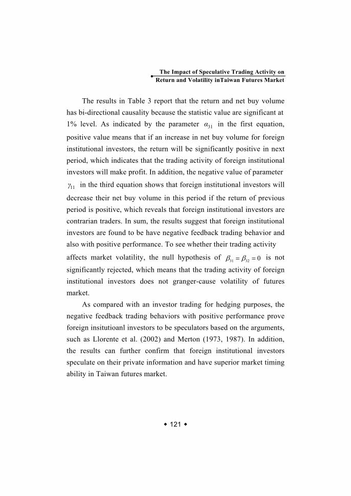
121
The Impact of Speculative Trading Activity on Return and Volatility inTaiwan Futures Market ‧
The results in Table 3 report that the return and net buy volume has bi-directional causality because the statistic value are significant at 1% level. As indicated by the parameter 31α in the first equation,
positive value means that if an increase in net buy volume for foreign institutional investors, the return will be significantly positive in next period, which indicates that the trading activity of foreign institutional investors will make profit. In addition, the negative value of parameter
11γ in the third equation shows that foreign institutional investors will
decrease their net buy volume in this period if the return of previous period is positive, which reveals that foreign institutional investors are contrarian traders. In sum, the results suggest that foreign institutional investors are found to be have negative feedback trading behavior and also with positive performance. To see whether their trading activity
affects market volatility, the null hypothesis of 31 32 0= =β β is not
significantly rejected, which means that the trading activity of foreign institutional investors does not granger-cause volatility of futures market.
As compared with an investor trading for hedging purposes, the negative feedback trading behaviors with positive performance prove foreign insitutioanl investors to be speculators based on the arguments, such as Llorente et al. (2002) and Merton (1973, 1987). In addition, the results can further confirm that foreign institutional investors speculate on their private information and have superior market timing ability in Taiwan futures market.
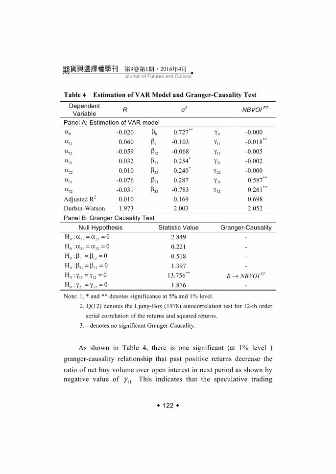
122
Journal of Futures and Options期貨與選擇權學刊 第9卷第1期 201‧ 6年4月
‧
Table 4 Estimation of VAR Model and Granger-Causality Test Dependent
Variable R σ2 NBVOI FT
Panel A: Estimation of VAR model
0α -0.020 0β 0.727** 0γ -0.000
11α 0.060 11β -0.103 11γ -0.018**
12α -0.059 12β -0.068 12γ -0.005 21α 0.032 21β 0.254*
21γ -0.002 22α 0.010 22β 0.240*
22γ -0.000 31α -0.076 31β 0.287 31γ 0.587**
32α -0.031 32β -0.783 32γ 0.261**
Adjusted R2 0.010 0.169 0.698 Durbin-Watson 1.973 2.003 2.052 Panel B: Granger Causality Test
Null Hypothesis Statistic Value Granger-Causality
0 21 22H : 0α = α = 2.849 - 0 31 32H : 0α = α = 0.221 - 0 11 12H : 0β = β = 0.518 - 0 31 32H : 0β = β = 1.397 - 0 11 12H : 0γ = γ = 13.756** FTR NBVOI→ 0 21 22H : 0γ = γ = 1.876 -
Note: 1. * and ** denotes significance at 5% and 1% level. 2. Q(12) denotes the Ljung-Box (1978) autocorrelation test for 12-th order
serial correlation of the returns and squared returns. 3. - denotes no significant Granger-Causality.
As shown in Table 4, there is one significant (at 1% level )
granger-causality relationship that past positive returns decrease the ratio of net buy volume over open interest in next period as shown by negative value of 11γ . This indicates that the speculative trading
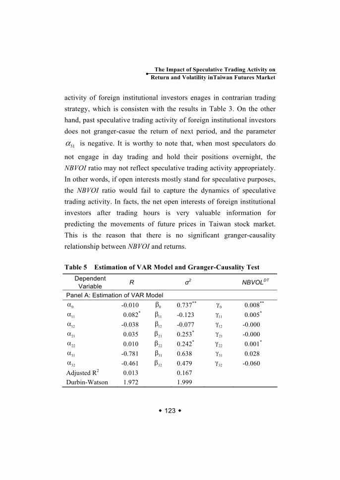
123
The Impact of Speculative Trading Activity on Return and Volatility inTaiwan Futures Market ‧
activity of foreign institutional investors enages in contrarian trading strategy, which is consisten with the results in Table 3. On the other hand, past speculative trading activity of foreign institutional investors does not granger-casue the return of next period, and the parameter
31α is negative. It is worthy to note that, when most speculators do
not engage in day trading and hold their positions overnight, the NBVOI ratio may not reflect speculative trading activity appropriately. In other words, if open interests mostly stand for speculative purposes, the NBVOI ratio would fail to capture the dynamics of speculative trading activity. In facts, the net open interests of foreign institutional investors after trading hours is very valuable information for predicting the movements of future prices in Taiwan stock market. This is the reason that there is no significant granger-causality relationship between NBVOI and returns.
Table 5 Estimation of VAR Model and Granger-Causality Test
Dependent Variable R σ2 NBVOLDT
Panel A: Estimation of VAR Model
0α -0.010 0β 0.737** 0γ 0.008**
11α 0.082* 11β -0.123 11γ 0.005*
12α -0.038 12β -0.077 12γ -0.000 21α 0.035 21β 0.253*
21γ -0.000 22α 0.010 22β 0.242*
22γ 0.001*
31α -0.781 31β 0.638 31γ 0.028 32α -0.461 32β 0.479 32γ -0.060
Adjusted R2 0.013 0.167 Durbin-Watson 1.972 1.999
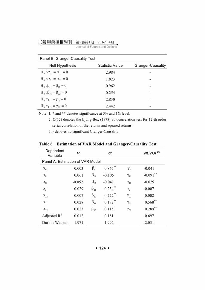
124
Journal of Futures and Options期貨與選擇權學刊 第9卷第1期 201‧ 6年4月
‧
Panel B: Granger Causality Test
Null Hypothesis Statistic Value Granger-Causality
0 21 22H : 0α = α = 2.984 -
0 31 32H : 0α = α = 1.823 -
0 11 12H : 0β = β = 0.962 -
0 31 32H : 0β = β = 0.254 -
0 11 12H : 0γ = γ = 2.830 -
0 21 22H : 0γ = γ = 2.442 -
Note: 1. * and ** denotes significance at 5% and 1% level. 2. Q(12) denotes the Ljung-Box (1978) autocorrelation test for 12-th order
serial correlation of the returns and squared returns. 3. - denotes no significant Granger-Causality.
Table 6 Estimation of VAR Model and Granger-Causality Test
Dependent Variable R σ2 NBVOI DT
Panel A: Estimation of VAR Model
0α 0.003 0β 0.865** 0γ -0.041
11α 0.061 11β -0.105 11γ -0.091**
12α -0.052 12β -0.041 12γ -0.029
21α 0.029 21β 0.234** 21γ 0.007
22α 0.007 22β 0.222** 22γ 0.002
31α 0.028 31β 0.182** 31γ 0.568**
32α 0.023 32β 0.115 32γ 0.289**
Adjusted R2 0.012 0.181 0.697
Durbin-Watson 1.971 1.992 2.031
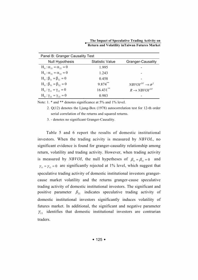
125
The Impact of Speculative Trading Activity on Return and Volatility inTaiwan Futures Market ‧
Panel B: Granger Causality Test Null Hypothesis Statistic Value Granger-Causality
0 21 22H : 0α = α = 1.995 - 0 31 32H : 0α = α = 1.243 - 0 11 12H : 0β = β = 0.458 - 0 31 32H : 0β = β = 9.874** 2DTNBVOI σ→ 0 11 12H : 0γ = γ = 16.431** DTR NBVOI→ 0 21 22H : 0γ = γ = 0.983 -
Note: 1. * and ** denotes significance at 5% and 1% level. 2. Q(12) denotes the Ljung-Box (1978) autocorrelation test for 12-th order
serial correlation of the returns and squared returns. 3. - denotes no significant Granger-Causality.
Table 5 and 6 report the results of domestic institutional
investors. When the trading acivity is measured by NBVOL, no significant evidence is found for granger-causality relationship among return, volatility and trading activity. However, when trading activity is measured by NBVOI, the null hypetheses of 31 32 0 β β= = and
11 12 0 γ γ= = are significantly rejected at 1% level, which suggest that
speculative trading activity of domestic institutional investors granger-cause market volatility and the returns granger-cause speculative trading activity of domestic institutional investors. The significant and positive parameter 31β indicates speculative trading activity of
domestic institutional investors significantly induces volatility of futures market. In additional, the significant and negative parameter
11γ identifies that domestic institutional investors are contrarian
traders.
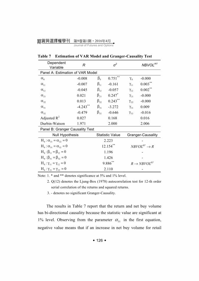
126
Journal of Futures and Options期貨與選擇權學刊 第9卷第1期 201‧ 6年4月
‧
Table 7 Estimation of VAR Model and Granger-Causality Test Dependent
Variable R σ2 NBVOLRT
Panel A: Estimation of VAR Model
0α -0.008 0β 0.751** 0γ -0.000
11α -0.007 11β -0.161 11γ 0.003**
12α -0.045 12β -0.057 12γ 0.002**
21α 0.021 21β 0.247* 21γ -0.000
22α 0.013 22β 0.243** 22γ -0.000
31α -4.243** 31β -3.272 31γ 0.009
32α -0.479 32β -0.646 32γ -0.016 Adjusted R2 0.027 0.168 0.016 Durbin-Watson 1.971 2.000 2.006 Panel B: Granger Causality Test
Null Hypothesis Statistic Value Granger-Causality
0 21 22H : 0α = α = 2.223 - 0 31 32H : 0α = α = 12.154** RTNBVOL R→ 0 11 12H : 0β = β = 1.196 - 0 31 32H : 0β = β = 1.426 - 0 11 12H : 0γ = γ = 9.886** RTR NBVOL→ 0 21 22H : 0γ = γ = 2.110 -
Note: 1. * and ** denotes significance at 5% and 1% level. 2. Q(12) denotes the Ljung-Box (1978) autocorrelation test for 12-th order
serial correlation of the returns and squared returns. 3. - denotes no significant Granger-Causality.
The results in Table 7 report that the return and net buy volume
has bi-directional causality because the statistic value are significant at
1% level. Observing from the parameter 31α in the first equation,
negative value means that if an increase in net buy volume for retail
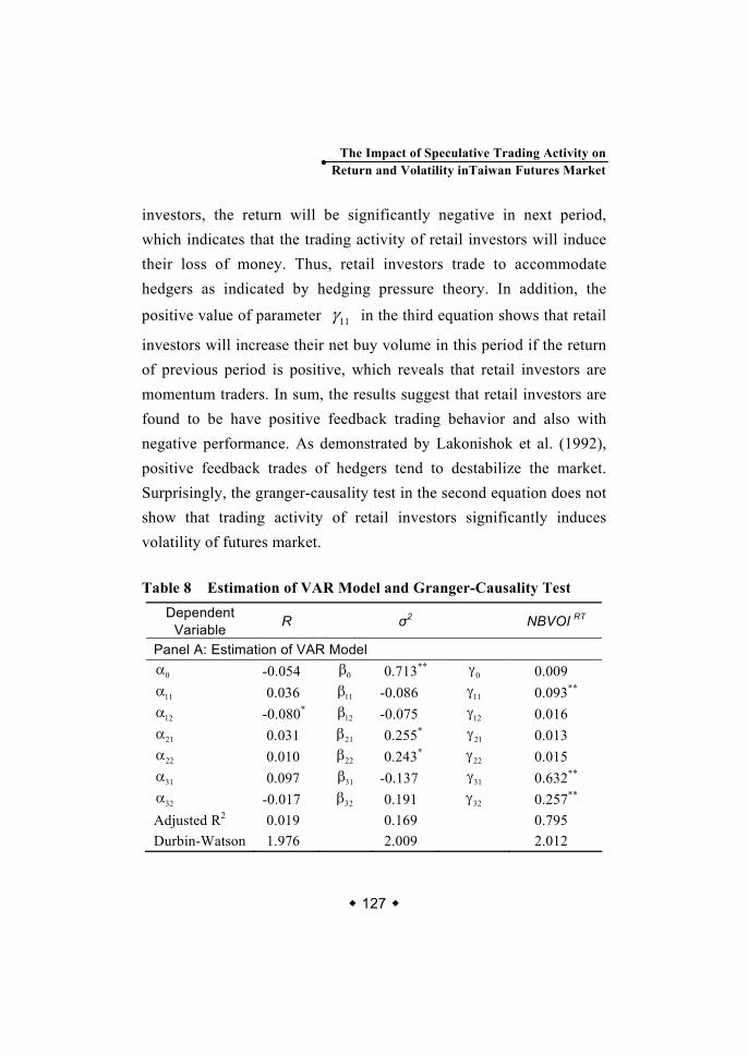
127
The Impact of Speculative Trading Activity on Return and Volatility inTaiwan Futures Market ‧
investors, the return will be significantly negative in next period, which indicates that the trading activity of retail investors will induce their loss of money. Thus, retail investors trade to accommodate hedgers as indicated by hedging pressure theory. In addition, the
positive value of parameter 11γ in the third equation shows that retail
investors will increase their net buy volume in this period if the return of previous period is positive, which reveals that retail investors are momentum traders. In sum, the results suggest that retail investors are found to be have positive feedback trading behavior and also with negative performance. As demonstrated by Lakonishok et al. (1992), positive feedback trades of hedgers tend to destabilize the market. Surprisingly, the granger-causality test in the second equation does not show that trading activity of retail investors significantly induces volatility of futures market. Table 8 Estimation of VAR Model and Granger-Causality Test
Dependent Variable R σ2 NBVOI RT
Panel A: Estimation of VAR Model
0α -0.054 0β 0.713** 0γ 0.009
11α 0.036 11β -0.086 11γ 0.093**
12α -0.080* 12β -0.075 12γ 0.016
21α 0.031 21β 0.255* 21γ 0.013
22α 0.010 22β 0.243* 22γ 0.015
31α 0.097 31β -0.137 31γ 0.632**
32α -0.017 32β 0.191 32γ 0.257**
Adjusted R2 0.019 0.169 0.795 Durbin-Watson 1.976 2.009 2.012
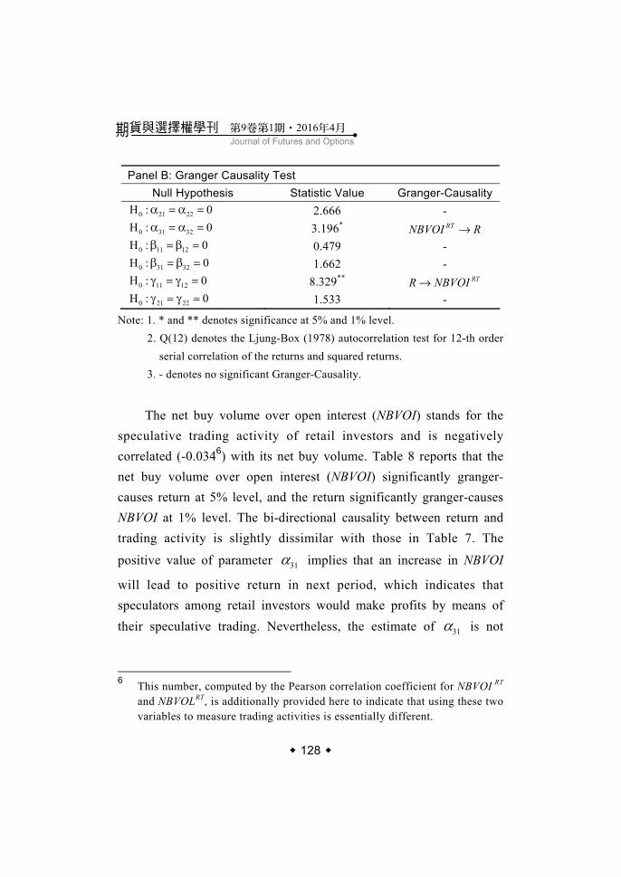
128
Journal of Futures and Options期貨與選擇權學刊 第9卷第1期 201‧ 6年4月
‧
Panel B: Granger Causality Test Null Hypothesis Statistic Value Granger-Causality
0 21 22H : 0α = α = 2.666 - 0 31 32H : 0α = α = 3.196* RTNBVOI R→ 0 11 12H : 0β = β = 0.479 - 0 31 32H : 0β = β = 1.662 - 0 11 12H : 0γ = γ = 8.329** RTR NBVOI→ 0 21 22H : 0γ = γ = 1.533 -
Note: 1. * and ** denotes significance at 5% and 1% level. 2. Q(12) denotes the Ljung-Box (1978) autocorrelation test for 12-th order
serial correlation of the returns and squared returns. 3. - denotes no significant Granger-Causality.
The net buy volume over open interest (NBVOI) stands for the
speculative trading activity of retail investors and is negatively correlated (-0.0346) with its net buy volume. Table 8 reports that the net buy volume over open interest (NBVOI) significantly granger-causes return at 5% level, and the return significantly granger-causes NBVOI at 1% level. The bi-directional causality between return and trading activity is slightly dissimilar with those in Table 7. The
positive value of parameter 31α implies that an increase in NBVOI
will lead to positive return in next period, which indicates that speculators among retail investors would make profits by means of their speculative trading. Nevertheless, the estimate of 31α is not
6 This number, computed by the Pearson correlation coefficient for NBVOI RT
and NBVOLRT, is additionally provided here to indicate that using these two variables to measure trading activities is essentially different.
129
The Impact of Speculative Trading Activity on Return and Volatility inTaiwan Futures Market ‧
significant. On the other hand, the positive value of parameter 11γ
also suggests that speculators among retail investors tend to be momentum traders. Similarly, the speculative trading activity of retail investors will not cause market instability.
IV. Conclusion
The study examines the relationsip among return, volatility and trading activity of trader type in Taiwan futures market. The trading activity of trader type is measured by two proxies, i.e. the net buy volume and the ratio of trading volume over open interest. As suggested by Garcia et al. (1986) and Luu and Martens (2003), this ratio can alleviate possible time effect on trading activity and capture information arrivals. Thus, we expect that using this alternative manner to examine the performance of trader type and their trading behaviors might provide more insights about hedging pressure effect and market timing ability possessed by trader types in Taiwan futures market.
The empirical results show that there are some discrepancies when trading volume and trading volume over open interest are used as the proxy of trading activity. Irrespective of trading activity proxy, the foreign institutional investors are contrarian traders and retail investors are momentum traders. For domestic institutional investors, they engage in contrarian trading when using net buy volume over open interest to proxy their trading activity. In addition, the results of net buy volume indicate that foreign institutional investors tend to make profit and retail investors tend to lose money. However, no

130
Journal of Futures and Options期貨與選擇權學刊 第9卷第1期 201‧ 6年4月
‧
significant evidence shows that speculative trading activities of foreign institutional and retail investors make or lose money. As for the impacts of trading activity on volatility, only speculative trading of domestic institutional investors destabilizes the futures market.
As indicated by the hedging pressure theory, hegders are required to pay a significant premium to speculators for bearing risk, and thus their position changes are negatively correlated with subsequent futures return. In contrast, the position changes of speculators are positively with subsequent futures price movements. This study concludes that foreign institutional investors are speculators and retail investors are hedgers in Taiwan futures market. Our findings are consistent with Wang (2003), which suggests that speculators are contrarian traders.
It is well-known that institutional investors often engage in trading activity with diverse financial instruments in multiple markets simultaneously. Thus, this paper would like to remind that the conclusions are merely drawn in the context regarding (speculative) trading activity of trader type on return and volatility in Taiwan futures market.
131
The Impact of Speculative Trading Activity on Return and Volatility inTaiwan Futures Market ‧
References
Andersen, T. G., T. Bollerslev, F. X. Diebold and H. Ebens (2001), “The Distribution of Realized Stock Return Volatility,” Journal of Financial Economics, 61(1), 43-76. Bessembinder, H. and P. Seguin (1992), “Futures-Trading Activity and Stock Price Volatility,” Journal of Finance, 47, 2015-2034. Bessembinder, H. and P. Seguin (1993), “Price Volatility, Trading Volume, and Market Depth: Evidence from Futures Markets,” Journal of Financail and Quantitative Analysis, 28(1), 21-39. Chatrath, A., S. Ramchander and F. Song (1995), “Does Options Trading Lead to Greater Cash Market Volatility?” Journal of Future Markets, 15, 785-803. Chatrath, A., S. Ramchander and F. Song (1996), “The Role of Futures Trading Activity in Exchange Rate Volatility,” Journal of Futures Markets, 16, 561-584. Chatrath, A., R. A. Christie-David, V. Lugli and C. Santoso (2010), “Futures Trading and Oil Price Movements,” Review of Futures Markets, 18, 347-362. Chang, Y. K., Y. L. Chen, R. K. Chou and Y. F. Gau (2013), “The Effectiveness of Position Limits: Evidence from the Foreign Exchange Futures Markets,” Journal of Banking and Finance, 37, 4501-4509. Cheng, T. Y., C. H. Lin and S. S. Chuang (2007), “Who is the Winner? Trading Behavior and Performance for Major Types of Traders—Evidence from Taiwan’s Futures Market,” Asia Pacific Management Review, 12(1), 13-21. Chiang, S. J., L. J. Tsai, P. G. Shu and S. L. Chen (2012), “The
132
Journal of Futures and Options期貨與選擇權學刊 第9卷第1期 201‧ 6年4月
‧
Trading Behavior of Foreign, Domestic Institutional, and Domestic Individual Investors: Evidence from Taiwan Stock Market,” Pacific-Basin Finance Journal, 20(5), 745-754. Fleming, J., C. Kirby and B. Ostdiek (2003), “The Economic Value of Volatility Timing Using ‘Realized’ Volatility,” Journal of Financial Economics, 67(3), 473-509. Gallant, A. R., P. E. Rossi and G. Tauchen (1992), “Stock Prices and Volume,” Review of Financial Studies, 5, 199-242. Garcia, P., R. Leuthold and H. Zapata (1986), “Lead-Lag Relationships between Trading Volume and Price Variability: New Evidence,” Journal of Futures Markets, 6, 1-10. Hagelin, N. (2000), “Index Option Market Activity and Cash Market Volatility under Different Market Conditions: An Empirical Study from Sweden,” Applied Financial Economics, 10, 597-613. Hansen, B. E. and B. Seo (2002), “Testing for Two-Regime Threshold Cointegration in Vector Error-Correction Models,” Journal of Econometrics, 110, 293-318. Huang, Y. C. (2002), “Trading Activity in Stock Index Futures Markets: The Evidence of Emerging Markets,” Journal of Futures Markets, 22(10), 983-1003. Kyriacou, K. and L. Sarno (1999), “The Temporal Relationship between Derivatives Trading and Spot Market Volatility in the UK: Empirical Analysis and Monte Carlo Evidence,” Journal of Futures Markets, 19, 245-270. Koopman, S. J., B. Jungbacker and E. Hol (2005), “Forecasting Daily Variability of the S&P 100 Stock Index Using Historical, Realized and Implied Volatility Measurements,” Journal of Empirical Finance, 12(3), 445-475.
133
The Impact of Speculative Trading Activity on Return and Volatility inTaiwan Futures Market ‧
Kuo, W. H., H. Hsu and C. Y. Chiang (2005), “Price Volatility, Trading Activity and Market Depth: Evidence from Taiwan and Singapore Taiwan Stock Index Futures Markets,” Asia Pacific Management Review, 10(1), 131-143. Kurov, A. (2008), “Investor Sentiment, Trading Behavior and Information Efficiency in Index Futures Markets,” Financial Review, 43, 107-127. Lakonishok, J., A. Shleifer and R. W. Vishny (1992), “The Impact of Institutional Trading on Stock Prices,” Journal of Financial Economics, 32, 23-43. Lee, Y. T., J. C. Lin and Y. J. Liu (1999), “Trading Patterns of Big versus Small Players in an Emerging Market: An Empirical Analysis,” Journal of Banking and Finance, 23, 701-725. Luu, J. C. and M. Martens (2003), “Testing the Mixture-of-Distributions Hypothesis Using Realized Volatility,” Journal of Futures Markets, 23, 661-679. Llorente, G., R. Michaely, G. Saar and J. Wang (2002), “Dynamic Volume-Return Relation of Individual Stocks,” Review of Financial Studies, 15(4), 1005-1047. Merton, R. (1973), “An Intertemporal Capital Asset Pricing Model,” Econometrica, 41, 867-887. Merton, R. (1987), “A Simple Model of Capital Market Equilibrium with Incomplete Information,” Journal of Finance, 42, 483-451. Parkinson, M. (1980), “The Extreme Value Method for Estimating the Variance of the Rate of Return,” Journal Business, 53, 61-65. Röthig, A. and C. Chiarella (2007), “Investigating Nonlinear Speculation in Cattle, Corn, and Hog Futures Markets Using Logistic Smooth Transition Regression Models,” Journal of Futures Markets,
134
Journal of Futures and Options期貨與選擇權學刊 第9卷第1期 201‧ 6年4月
‧
27, 719-737. Sanders, D. R., K. Boris and M. Manfredo (2004), “Hedgers, Funds, and Small Speculators in the Energy Futures Markets: An Analysis of the CFTC’s Commitments of Traders Reports,” Energy Economics, 26, 425-445. Wang, C. (2003), “The Behavior and Performance of Major Types of Futures Traders,” Journal of Futures Markets, 23, 1-31. Wang, C. and M. Yu (2004), “Trading Activity and Price Reversals in Futures Markets,” Journal of Banking and Finance, 28(6), 1337-1361. Wang, C. (2004), “Futures Trading Activity and Predictable Foreign Exchange Market Movements,” Journal of Banking and Finance, 28(6), 1337-1361.

「期貨與選擇權學刊」 徵稿簡則
一、本刊徵求有關期貨、選擇權或衍生性商品理論與實證或應用之
中、英文學術論文。 二、來稿請惠寄一式四份,其中兩份請採不具姓名方式,本刊將送
請相關領域學者專家審閱後向編輯委員會作適當推薦。 三、來稿經本刊發表後,其著作權歸屬於本公司,非徵得同意,不
得轉載其他學術刊物。本公司並得以光碟或紙本方式重製、發
行,或發表於本公司網站上,及再授權國家圖書館或資料庫業
者,進行數位化典藏、重製、透過網路公開傳輸、授權用戶下
載、列印瀏覽等服務。 四、已投寄其他學術期刊或已出版之論文請勿投稿本刊。 五、來稿長度以不超過2萬字為原則。稿件格式及文獻寫法請參考
「期貨與選擇權學刊論文格式說明」,中、英文稿請以word 7.0或PDF處理。
六、論文排版後之校對,由作者負責。惟本刊有權在摘要文字與規
格上酌予修改。 七、來稿刊登後,由本刊致贈學刊一份,並致贈稿酬新臺幣1萬元。
本規定自2013年11月20日起生效,生效日後投稿者(以郵戳或
電子郵件收件日為憑),適用新規定。 八、本刊自2014年起改為每年4、8、12月出刊三期,請踴躍投稿。
來稿請寄:100台北市中正區羅斯福路二段100號14樓 臺灣期貨
交易所 期貨與選擇權學刊收。

「期貨與選擇權學刊」 評審程序
本學刊之評審程序採雙向匿名審查制,以求審查過程之公正
客觀。學刊於接獲投稿後,如總編輯認為與本刊宗旨不符者,得
由總編輯逕行退件。符合本刊宗旨者,由總編輯就來稿性質諮詢
相關領域編輯委員之推薦,以指定評審人。每篇文稿至少由兩位
專家學者評審。評審人於評審意見表勾選下列選項之一,並陳述
意見以供作者修改。 不需修改即可刊登 適度修改再予重審 大幅修改再予重審 不推薦
1. 大部分承襲國內外研究,且無創新改進之處 2. 研究方法及觀點具有重大瑕疵 3. 研究結果在學術或應用上無參考價值 4. 其他(請說明)
評審後之文稿處理方式原則如下:
第二位評審意見
刊登 適度修改 大幅修改 不推薦
刊登 刊登 寄回修改 寄回修改 第三位評審
適度修改 寄回修改 寄回修改 寄回修改 第三位評審
大幅修改 寄回修改 寄回修改 退稿 退稿
第一位評審意見 不推薦 第三位評審 第三位評審 退稿 退稿
兩位評審人之意見若有重大差異,則另洽第三位評審人審
查。在另洽第三位評審之情況下,若第三位評審之意見為「刊
登」或「適修」時,則寄回作者修改後再送審;如第三位評審之
意見為「大修」或「不推薦」,則予以退稿。所有評審結果及審
查意見將函送投稿人。
文稿
處理方式

「期貨與選擇權學刊」 論文格式說明
內 容
本刊徵求有關國內外期貨、選擇權或衍生性商品及其法律規
範與制度之理論、實證或應用之中。英文學術論文。來稿請
以中文或英文數字(Times New Roman)撰寫,一律使用A4
紙張,由左而右橫式打字,並依下列順序書寫並依順序編入
頁碼:封面頁(含標題、作者、服務機構。中英文摘要、關
鍵詞)、本文、注釋、圖表、附錄,及參考文獻。
篇 名
力求簡潔並能充分表達論文概念之描述性中、英文標題。
例:期貨市場的微觀結構
Microstructures of Futures Markets
作 者
姓名及服務機構完整中、英文名稱與地址。
摘 要
簡短中。英文摘要,以300字為原則。
關鍵詞
摘要之後請附3至5個中、英文關鍵詞(keywords)。
例:關鍵詞:期貨、市場流動性、避險者
Keywords: Futures, Market liquidity, Hedgers
章 節
章節款項,請依照「壹、一、(一)、1.、(1)」之順序排列,標
題請採用粗體。每段標題與子標題前請留一行空自。每一段
落首行以縮排2個中文(或全形)字元開始。

章節標號以中文撰寫者,如下列所示:
壹、前言(置中)
一、研究動機(置左)
(一)資料來源
1
(1) 章節標號以英文撰寫者,如下列所示:
I. Introduction
1.
1.1
1.1.1
圖 表
圖之標題置於圖下方,表之標題置於表上方,與圖、表之左
緣對齊。圖次、表次一律以阿拉伯數字表示。例如:圖1、表
1。圖寬以不超過內文寬度為主。表寬以對齊內文寬度為主。
引 註
自首頁(摘要頁)始,採隨文註腳(footnote)格式,註釋
列於各該頁下方,本文中以阿拉伯數字(不加括號)為
之,註在相關文字之右上方標點符號之前或後(段引
註)。文中如有參閱文獻部份,請以括弧夾註格式詳列來
源:(作者,年代)/作者(年代)。
法律類文章特有之引註文獻格式如下:
文章請以「」標示,書名請以劃底線標明,出版年份一
律使用西元紀元。引用大法官解釋、法律條文及行政函
示,無須註明日期及出處。引據外國法律法規、判決及
相關文獻時,請依各該國學術期刊成例。英文法律類論
文請依照Harvard Bluebook(Uniform Citation System)之
引註格式撰寫。

參考範例如下:
大法官解釋:大法官釋字第548號。
法律條文:著作權法第65條第2項第1款。
行政函示:公平會(89)公參字第89075481001號函。
法律判決:行政法院83年判字第56號、行政法裁判要
旨彙編,第14輯,966,1994。
法院決議:85年度第12次刑事庭決議,85年7月2日,
最高法院刑事庭決議彙編,第X卷第X期,1996。
網頁:http://www.ftc.gov.tw/,查訪日期:2004年11月1
日。
參考文獻
無論財金類或法律類文章,其參考文獻均以文後條列方式
逐條列出,中文列於前,英文列於後,不加編號,中文以
第一作者姓名筆劃排序,英文以第一作者last name字首排
序。論文正文中所引用之文獻皆須列於參考文獻中,且僅
有在文中引用過者方能列入參考文獻。文獻之出版年份請
使用西元紀元,一律以小括號內註明年份置於作者之後,
中文參考文獻格式如下:
專書:作者名(西元年),書名,出版地:出版者。
張傳章(2005),期貨與選擇權,台北:雙葉書廊。
期刊論文: 作者名(西元年),「篇名」,出處書名,刊
期,頁碼。
廖四郎、王昭文(2005),「利率、匯率及價格風險下遠期
價格樹狀模型」,財務金融學刊,第13卷第2期,29-70。
英文:
Author #l LastName, FirstName(s) and Author #2 FirstName(s)
LastName (year), “Title of the Article,” Title of Journal (in Ital-ic type), Volume and Number, Page Numbers.
參考範例如下:
Books:
Cohen, Kalman J., Steven F. Maier, Robert A. Schwartz and
David K. Whitcomb (1986), The Microstructure of Securites Markets, New Jersey: Prentice-Hall.
Journal Articles:
Brorsen, B. Wade (1989), “Liquidity Costs and Scalping Returns
in the Corn Futures Market,” Journal of Futures Markets, 9,
115-139. 學位論文及其他類型資料格式亦依循上列原則。