CHE334 Instrumentation and Process Control Lecture 13 & 14 Chapter 10 : Dynamics of First Order System

By Dr. Maria Mustafa

Department of Chemical Engineering

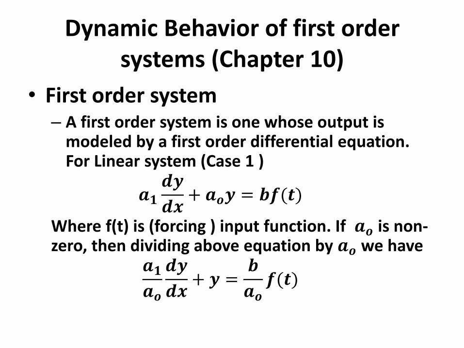
Dynamic Behavior of first order systems (Chapter 10)

• First order system – A first order system is one whose output is

modeled by a first order differential equation. For Linear system (Case 1 )

𝒂𝟏𝒅𝒚

𝒅𝒙+ 𝒂𝒐𝒚 = 𝒃𝒇(𝒕)

Where f(t) is (forcing ) input function. If 𝒂𝒐 is non-zero, then dividing above equation by 𝒂𝒐 we have

𝒂𝟏𝒂𝒐

𝒅𝒚

𝒅𝒙+ 𝒚 =

𝒃

𝒂𝒐𝒇(𝒕)

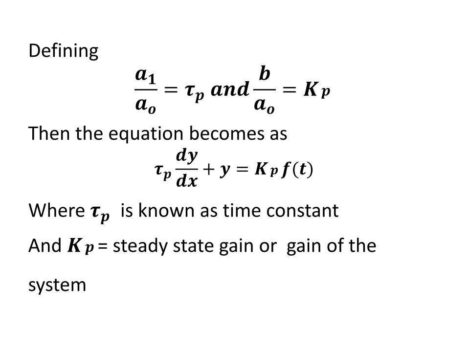
Defining 𝒂𝟏𝒂𝒐

= 𝝉𝒑 𝒂𝒏𝒅𝒃

𝒂𝒐= 𝑲𝒑

Then the equation becomes as

𝝉𝒑𝒅𝒚

𝒅𝒙+ 𝒚 = 𝑲𝒑𝒇(𝒕)

Where 𝝉𝒑 is known as time constant

And 𝑲𝒑 = steady state gain or gain of the

system

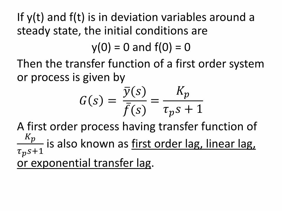
If y(t) and f(t) is in deviation variables around a steady state, the initial conditions are

y(0) = 0 and f(0) = 0

Then the transfer function of a first order system or process is given by

𝐺 𝑠 = 𝑦 (𝑠)

𝑓 (𝑠)=

𝐾𝑝𝜏𝑝𝑠 + 1

A first order process having transfer function of 𝐾𝑝

𝜏𝑝𝑠+1 is also known as first order lag, linear lag,

or exponential transfer lag.

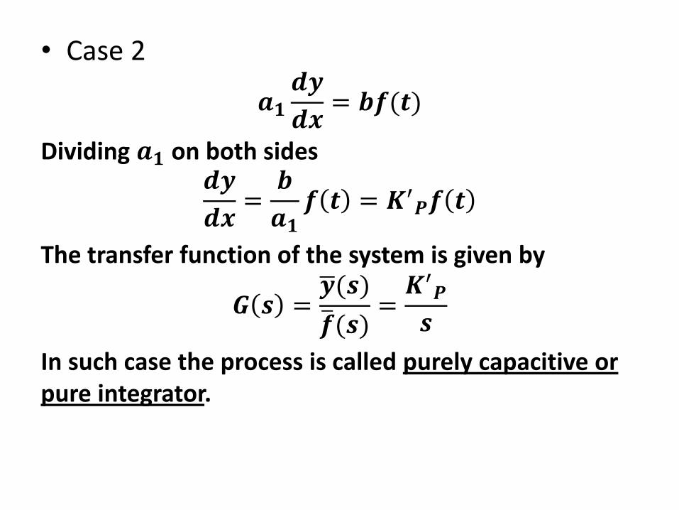
• Case 2

𝒂𝟏𝒅𝒚

𝒅𝒙= 𝒃𝒇(𝒕)

Dividing 𝒂𝟏 on both sides 𝒅𝒚

𝒅𝒙=

𝒃

𝒂𝟏𝒇 𝒕 = 𝑲′

𝑷𝒇 𝒕

The transfer function of the system is given by

𝑮 𝒔 =𝒚 (𝒔)

𝒇 (𝒔)=𝑲′

𝑷

𝒔

In such case the process is called purely capacitive or pure integrator.

Characteristics of First order System

• A process that possesses a capacity to tore mass or energy and then acts as a buffer between inflowing and outflowing streams will be ordered as first order system

• The first order processes are characterized by: – Their capacity to store mass, energy or

momentum. – The resistance associated with the flow of

mass. Energy or momentum in reaching the capacity.

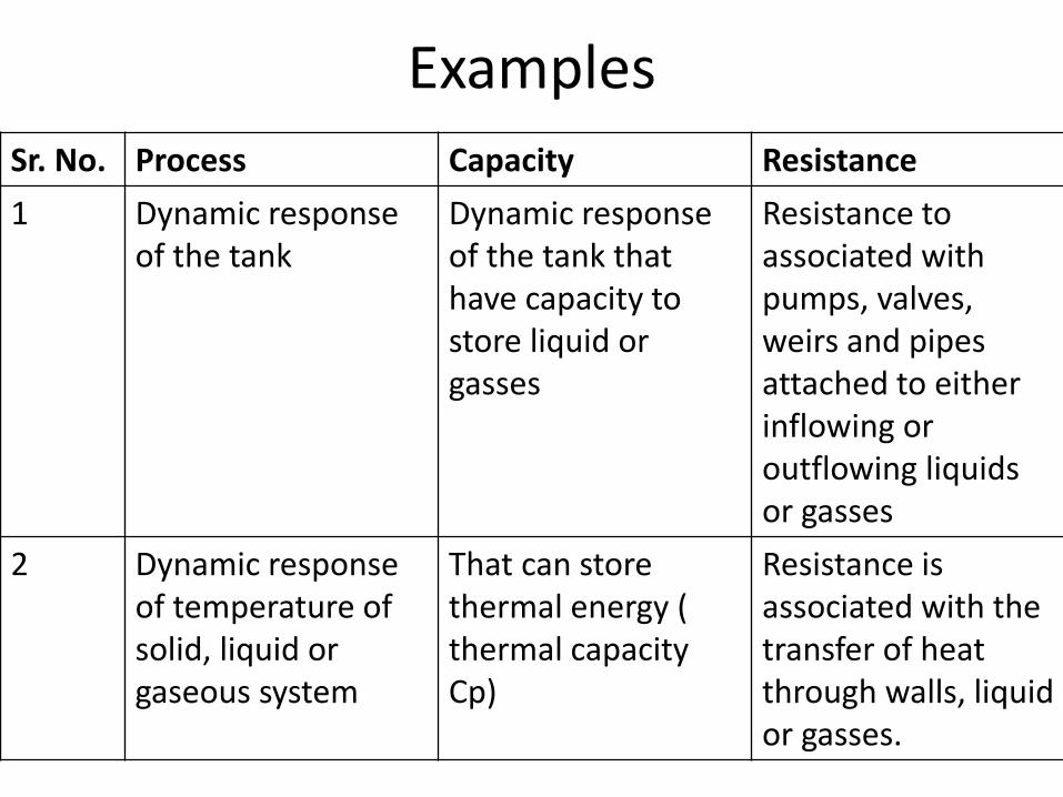
Examples

Sr. No. Process Capacity Resistance

1 Dynamic response of the tank

Dynamic response of the tank that have capacity to store liquid or gasses

Resistance to associated with pumps, valves, weirs and pipes attached to either inflowing or outflowing liquids or gasses

2 Dynamic response of temperature of solid, liquid or gaseous system

That can store thermal energy ( thermal capacity Cp)

Resistance is associated with the transfer of heat through walls, liquid or gasses.

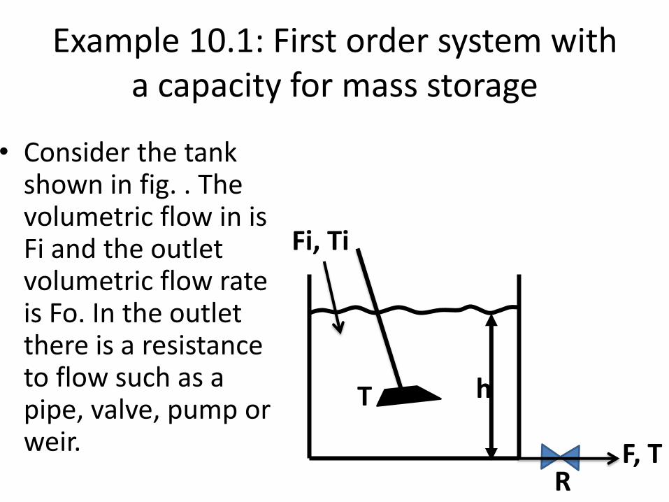
Example 10.1: First order system with a capacity for mass storage

• Consider the tank shown in fig. . The volumetric flow in is Fi and the outlet volumetric flow rate is Fo. In the outlet there is a resistance to flow such as a pipe, valve, pump or weir.

Fi, Ti

h

F, T

T

R

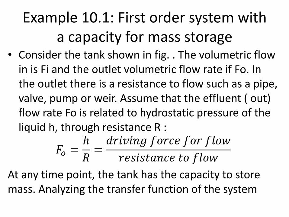
Example 10.1: First order system with a capacity for mass storage

• Consider the tank shown in fig. . The volumetric flow in is Fi and the outlet volumetric flow rate if Fo. In the outlet there is a resistance to flow such as a pipe, valve, pump or weir. Assume that the effluent ( out) flow rate Fo is related to hydrostatic pressure of the liquid h, through resistance R :

𝐹𝑜 =𝑕

𝑅=𝑑𝑟𝑖𝑣𝑖𝑛𝑔 𝑓𝑜𝑟𝑐𝑒 𝑓𝑜𝑟 𝑓𝑙𝑜𝑤

𝑟𝑒𝑠𝑖𝑠𝑡𝑎𝑛𝑐𝑒 𝑡𝑜 𝑓𝑙𝑜𝑤

At any time point, the tank has the capacity to store mass. Analyzing the transfer function of the system

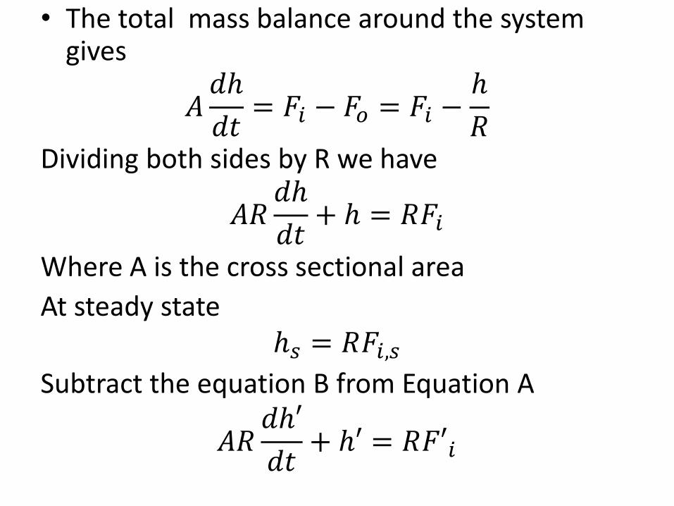
• The total mass balance around the system gives

𝐴𝑑𝑕

𝑑𝑡= 𝐹𝑖 − 𝐹𝑜 = 𝐹𝑖 −

𝑕

𝑅

Dividing both sides by R we have

𝐴𝑅𝑑𝑕

𝑑𝑡+ 𝑕 = 𝑅𝐹𝑖

Where A is the cross sectional area

At steady state 𝑕𝑠 = 𝑅𝐹𝑖,𝑠

Subtract the equation B from Equation A

𝐴𝑅𝑑𝑕′

𝑑𝑡+ 𝑕′ = 𝑅𝐹′𝑖

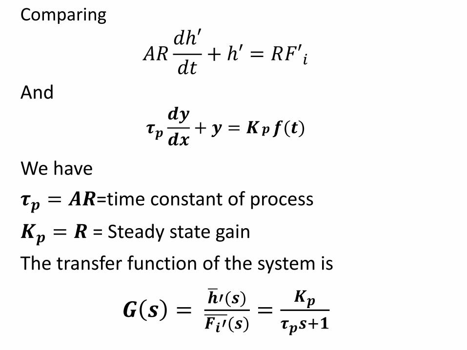
Comparing

𝐴𝑅𝑑𝑕′

𝑑𝑡+ 𝑕′ = 𝑅𝐹′𝑖

And

𝝉𝒑𝒅𝒚

𝒅𝒙+ 𝒚 = 𝑲𝒑𝒇(𝒕)

We have

𝝉𝒑 = 𝑨𝑹=time constant of process

𝑲𝒑 = 𝑹 = Steady state gain

The transfer function of the system is

𝑮 𝒔 = 𝒉 ′(𝒔)

𝑭𝒊′(𝒔)=

𝑲𝒑

𝝉𝒑𝒔+𝟏

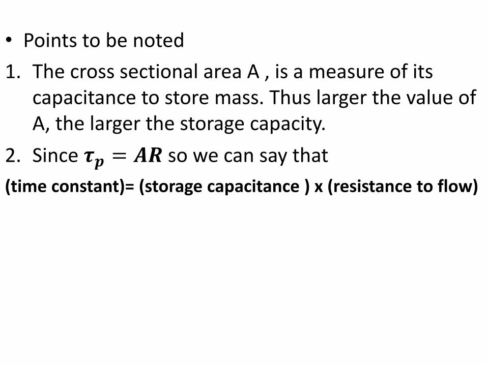
• Points to be noted

1. The cross sectional area A , is a measure of its capacitance to store mass. Thus larger the value of A, the larger the storage capacity.

2. Since 𝝉𝒑 = 𝑨𝑹 so we can say that

(time constant)= (storage capacitance ) x (resistance to flow)

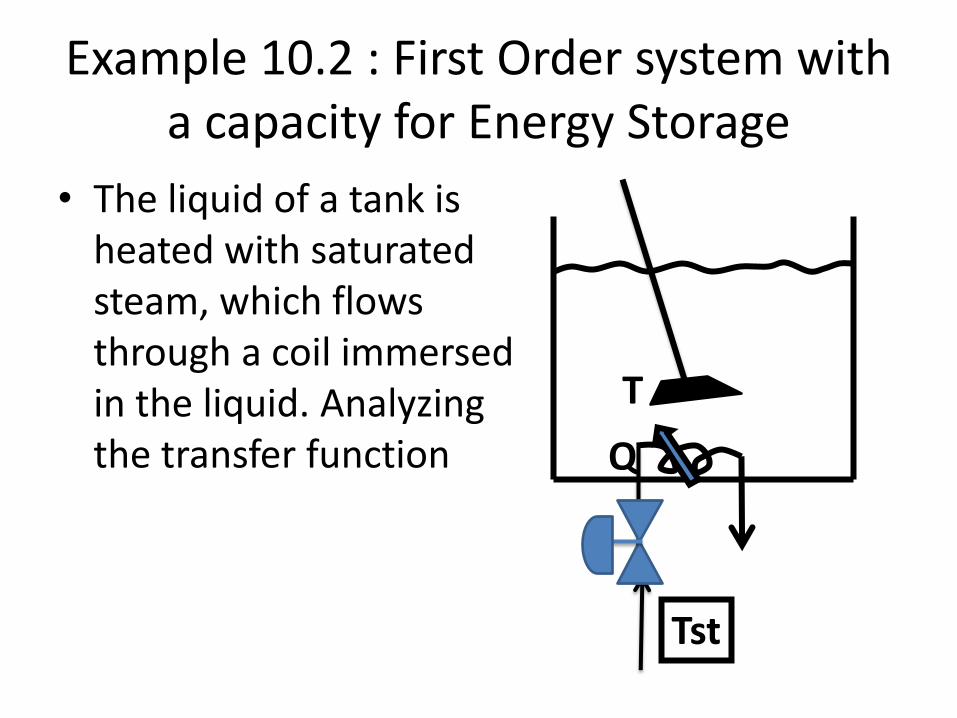
Example 10.2 : First Order system with a capacity for Energy Storage

• The liquid of a tank is heated with saturated steam, which flows through a coil immersed in the liquid. Analyzing the transfer function

Tst

T

Q

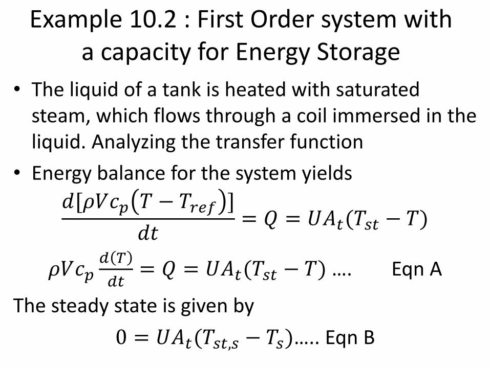
Example 10.2 : First Order system with a capacity for Energy Storage

• The liquid of a tank is heated with saturated steam, which flows through a coil immersed in the liquid. Analyzing the transfer function

• Energy balance for the system yields

𝑑[𝜌𝑉𝑐𝑝 𝑇 − 𝑇𝑟𝑒𝑓 ]

𝑑𝑡= 𝑄 = 𝑈𝐴𝑡(𝑇𝑠𝑡 − 𝑇)

𝜌𝑉𝑐𝑝𝑑 𝑇

𝑑𝑡= 𝑄 = 𝑈𝐴𝑡(𝑇𝑠𝑡 − 𝑇) …. Eqn A

The steady state is given by

0 = 𝑈𝐴𝑡(𝑇𝑠𝑡,𝑠 − 𝑇𝑠)….. Eqn B

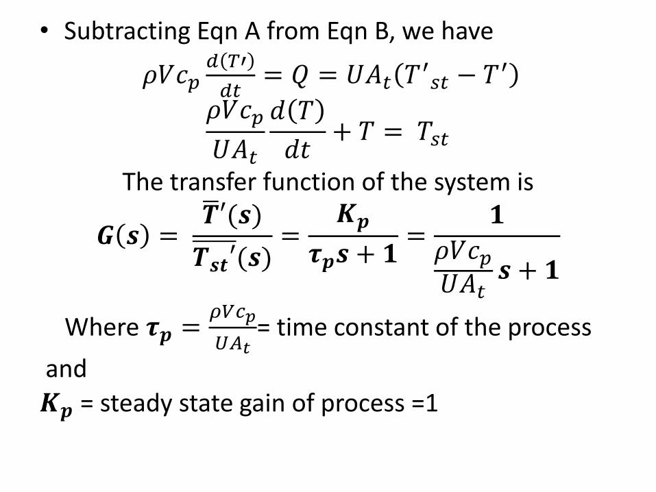
• Subtracting Eqn A from Eqn B, we have

𝜌𝑉𝑐𝑝𝑑 𝑇′

𝑑𝑡= 𝑄 = 𝑈𝐴𝑡 𝑇

′𝑠𝑡 − 𝑇′

𝜌𝑉𝑐𝑝

𝑈𝐴𝑡

𝑑 𝑇

𝑑𝑡+ 𝑇 = 𝑇𝑠𝑡

The transfer function of the system is

𝑮 𝒔 = 𝑻 ′(𝒔)

𝑻𝒔𝒕′(𝒔)=

𝑲𝒑

𝝉𝒑𝒔 + 𝟏=

𝟏

𝜌𝑉𝑐𝑝𝑈𝐴𝑡

𝒔 + 𝟏

Where 𝝉𝒑 =𝜌𝑉𝑐𝑝

𝑈𝐴𝑡= time constant of the process

and

𝑲𝒑 = steady state gain of process =1

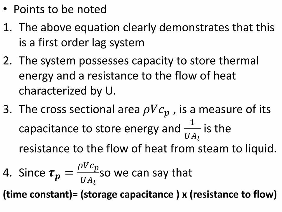
• Points to be noted

1. The above equation clearly demonstrates that this is a first order lag system

2. The system possesses capacity to store thermal energy and a resistance to the flow of heat characterized by U.

3. The cross sectional area 𝜌𝑉𝑐𝑝 , is a measure of its

capacitance to store energy and 1

𝑈𝐴𝑡 is the

resistance to the flow of heat from steam to liquid.

4. Since 𝝉𝒑 =𝜌𝑉𝑐𝑝

𝑈𝐴𝑡so we can say that

(time constant)= (storage capacitance ) x (resistance to flow)

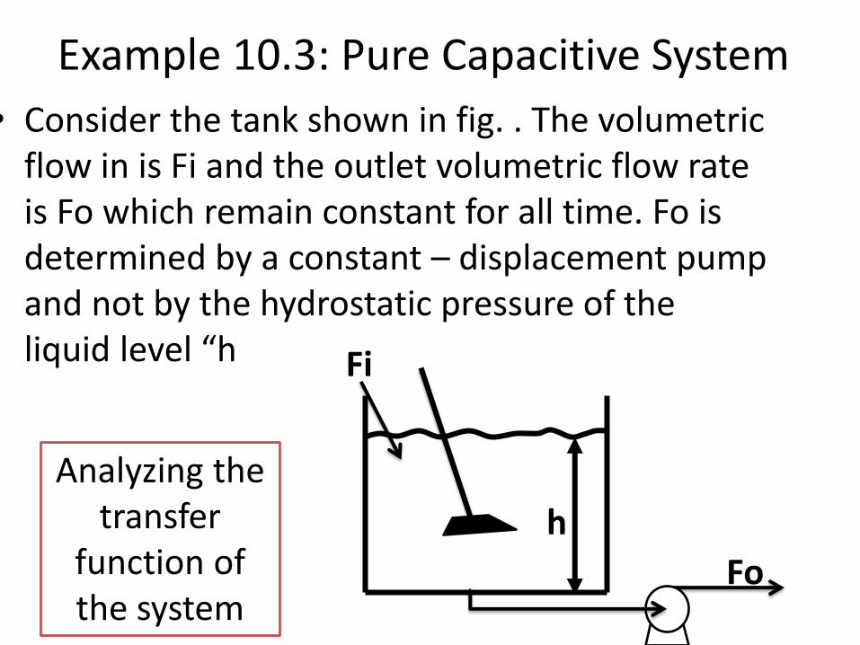
Example 10.3: Pure Capacitive System

• Consider the tank shown in fig. . The volumetric flow in is Fi and the outlet volumetric flow rate is Fo which remain constant for all time. Fo is determined by a constant – displacement pump and not by the hydrostatic pressure of the liquid level “h Fi

h

Fo

Analyzing the transfer

function of the system

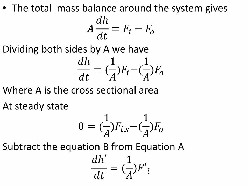
• The total mass balance around the system gives

𝐴𝑑𝑕

𝑑𝑡= 𝐹𝑖 − 𝐹𝑜

Dividing both sides by A we have 𝑑𝑕

𝑑𝑡= (

1

𝐴)𝐹𝑖−(

1

𝐴)𝐹𝑜

Where A is the cross sectional area

At steady state

0 = (1

𝐴)𝐹𝑖,𝑠−(

1

𝐴)𝐹𝑜

Subtract the equation B from Equation A 𝑑𝑕′

𝑑𝑡= (

1

𝐴)𝐹′𝑖

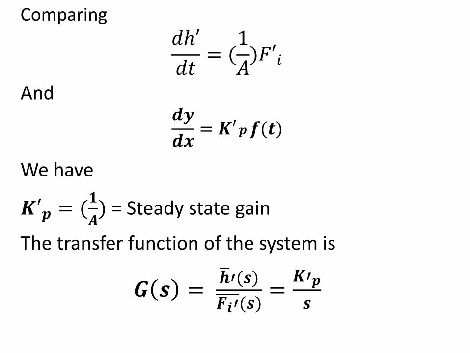
Comparing 𝑑𝑕′

𝑑𝑡= (

1

𝐴)𝐹′𝑖

And 𝒅𝒚

𝒅𝒙= 𝑲′𝒑𝒇(𝒕)

We have

𝑲′𝒑 = (𝟏

𝑨) = Steady state gain

The transfer function of the system is

𝑮 𝒔 = 𝒉 ′(𝒔)

𝑭𝒊′(𝒔)=

𝑲′𝒑

𝒔

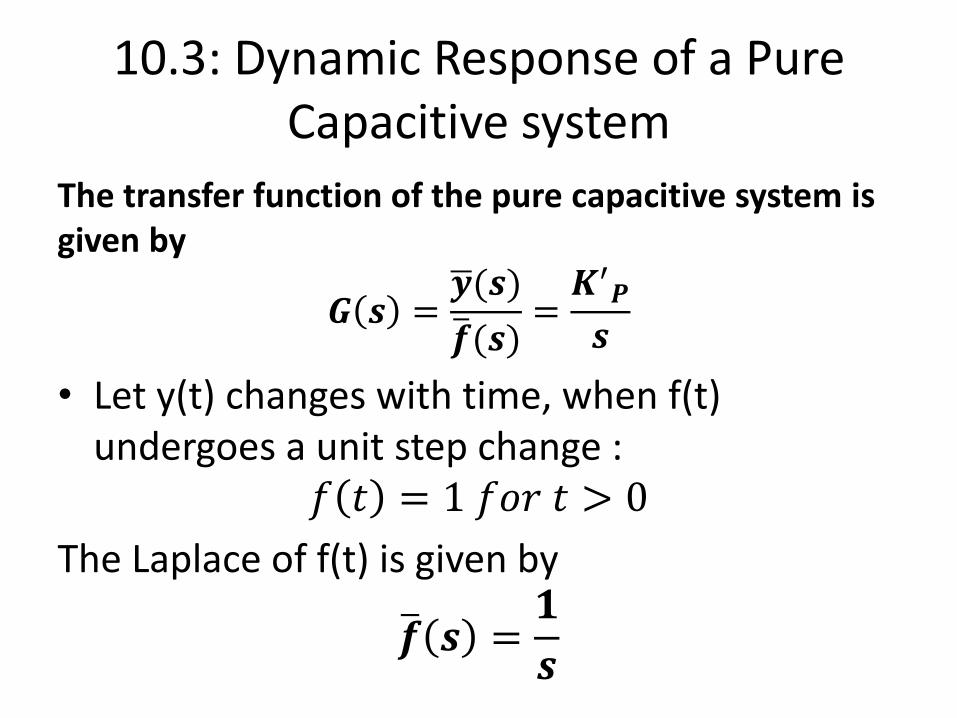
10.3: Dynamic Response of a Pure Capacitive system

The transfer function of the pure capacitive system is given by

𝑮 𝒔 =𝒚 (𝒔)

𝒇 (𝒔)=𝑲′

𝑷

𝒔

• Let y(t) changes with time, when f(t) undergoes a unit step change :

𝑓 𝑡 = 1 𝑓𝑜𝑟 𝑡 > 0

The Laplace of f(t) is given by

𝒇 𝒔 =𝟏

𝒔

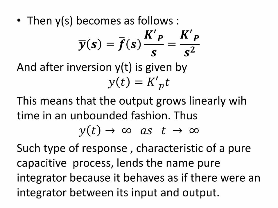
• Then y(s) becomes as follows :

𝒚 𝒔 = 𝒇 𝒔𝑲′

𝑷

𝒔=𝑲′

𝑷

𝒔𝟐

And after inversion y(t) is given by 𝑦 𝑡 = 𝐾′𝑝𝑡

This means that the output grows linearly wih time in an unbounded fashion. Thus

𝑦 𝑡 → ∞ 𝑎𝑠 𝑡 → ∞

Such type of response , characteristic of a pure capacitive process, lends the name pure integrator because it behaves as if there were an integrator between its input and output.

• A pure capacitive process can not balance itself, loose control and is known as non-self regulation process. It will cause serious control problems. As in example 10.3, a small change in inlet Flow will make the tank either flood or run dry (empty).

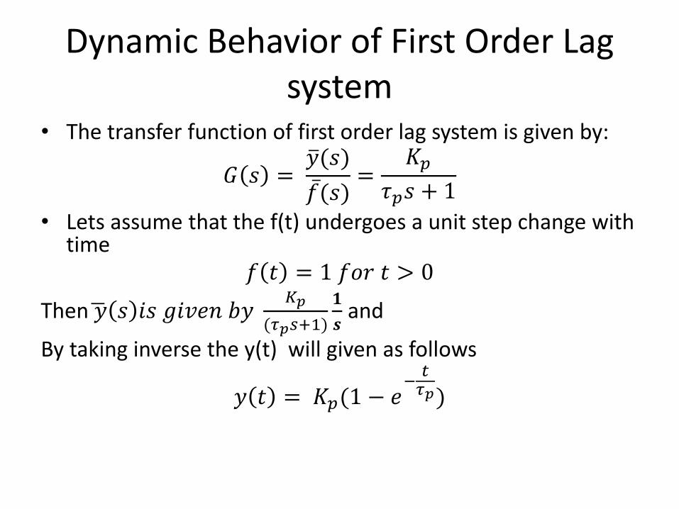
Dynamic Behavior of First Order Lag system

• The transfer function of first order lag system is given by:

𝐺 𝑠 = 𝑦 (𝑠)

𝑓 (𝑠)=

𝐾𝑝

𝜏𝑝𝑠 + 1

• Lets assume that the f(t) undergoes a unit step change with time

𝑓 𝑡 = 1 𝑓𝑜𝑟 𝑡 > 0

Then 𝑦 𝑠 𝑖𝑠 𝑔𝑖𝑣𝑒𝑛 𝑏𝑦 𝐾𝑝

(𝜏𝑝𝑠+1)

𝟏

𝒔 and

By taking inverse the y(t) will given as follows

𝑦 𝑡 = 𝐾𝑝(1 − 𝑒−𝑡𝜏𝑝)

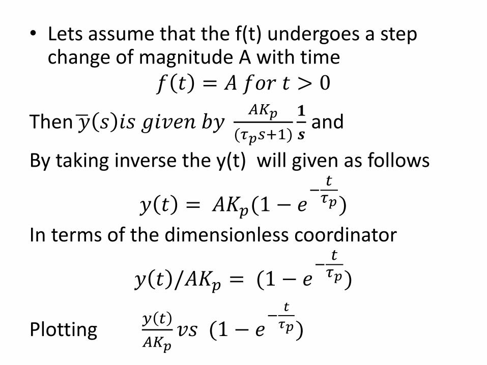
• Lets assume that the f(t) undergoes a step change of magnitude A with time

𝑓 𝑡 = 𝐴 𝑓𝑜𝑟 𝑡 > 0

Then 𝑦 𝑠 𝑖𝑠 𝑔𝑖𝑣𝑒𝑛 𝑏𝑦 𝐴𝐾𝑝

(𝜏𝑝𝑠+1)

𝟏

𝒔 and

By taking inverse the y(t) will given as follows

𝑦 𝑡 = 𝐴𝐾𝑝(1 − 𝑒−𝑡𝜏𝑝)

In terms of the dimensionless coordinator

𝑦 𝑡 /𝐴𝐾𝑝 = (1 − 𝑒−𝑡𝜏𝑝)

Plotting 𝑦 𝑡

𝐴𝐾𝑝𝑣𝑠 (1 − 𝑒

−𝑡

𝜏𝑝)

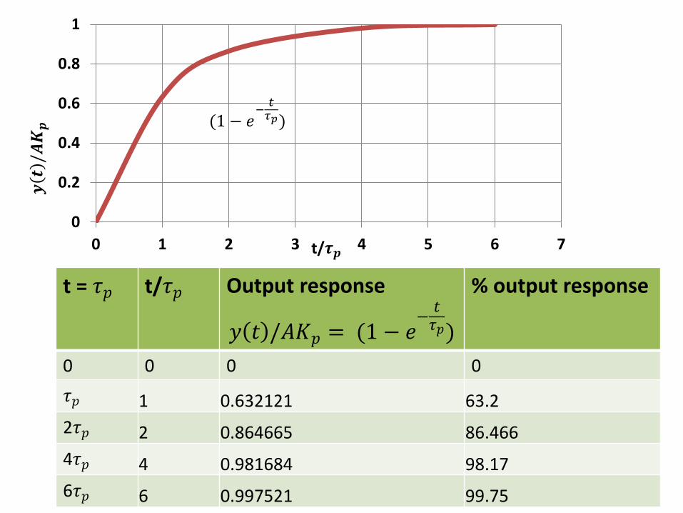
t = 𝜏𝑝 t/𝜏𝑝 Output response

𝑦 𝑡 /𝐴𝐾𝑝 = (1 − 𝑒−𝑡𝜏𝑝)

% output response

0 0 0 0

𝜏𝑝 1 0.632121 63.2

2𝜏𝑝 2 0.864665 86.466

4𝜏𝑝 4 0.981684 98.17

6𝜏𝑝 6 0.997521 99.75

0

0.2

0.4

0.6

0.8

1

0 1 2 3 4 5 6 7

(1 − 𝑒−𝑡𝜏𝑝)

𝒚𝒕/𝑨

𝑲𝒑

t/𝝉𝒑

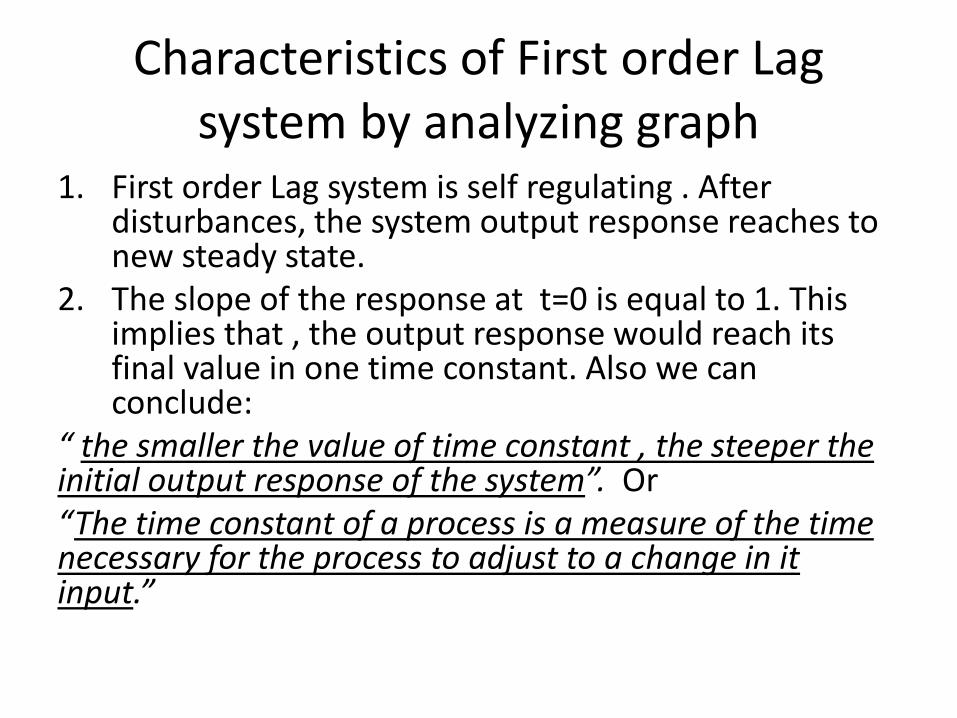
Characteristics of First order Lag system by analyzing graph

1. First order Lag system is self regulating . After disturbances, the system output response reaches to new steady state.

2. The slope of the response at t=0 is equal to 1. This implies that , the output response would reach its final value in one time constant. Also we can conclude:

“ the smaller the value of time constant , the steeper the initial output response of the system”. Or “The time constant of a process is a measure of the time necessary for the process to adjust to a change in it input.”

Characteristics of First order Lag system by analyzing graph

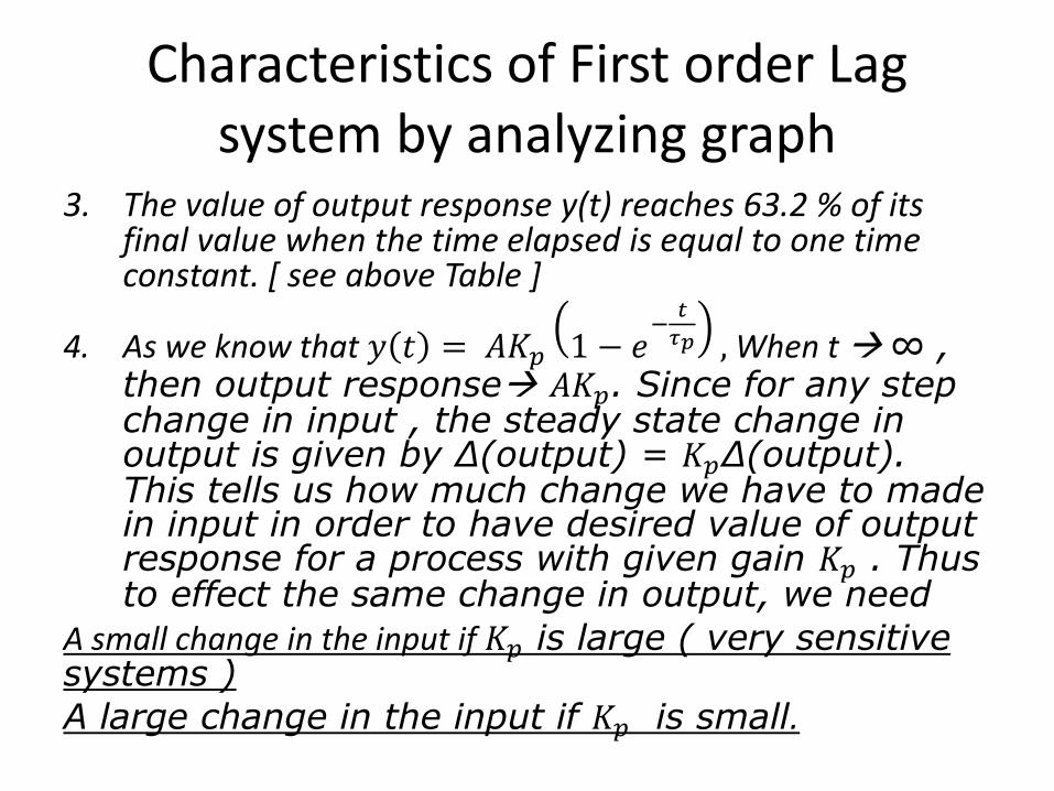
3. The value of output response y(t) reaches 63.2 % of its final value when the time elapsed is equal to one time constant. [ see above Table ]

4. As we know that 𝑦 𝑡 = 𝐴𝐾𝑝 1 − 𝑒−

𝑡

𝜏𝑝 , When t ∞ , then output response 𝐴𝐾𝑝. Since for any step change in input , the steady state change in output is given by ∆(output) = 𝐾𝑝∆(output). This tells us how much change we have to made in input in order to have desired value of output response for a process with given gain 𝐾𝑝 . Thus to effect the same change in output, we need

A small change in the input if 𝐾𝑝 is large ( very sensitive systems )

A large change in the input if 𝐾𝑝 is small.

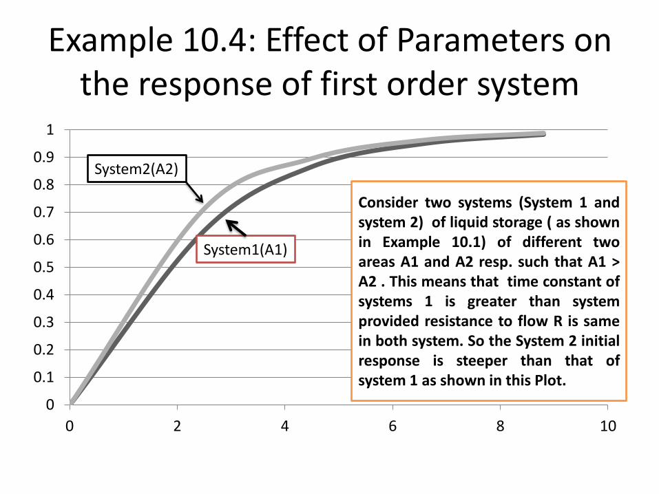
Example 10.4: Effect of Parameters on the response of first order system

0

0.1

0.2

0.3

0.4

0.5

0.6

0.7

0.8

0.9

1

0 2 4 6 8 10

Consider two systems (System 1 and system 2) of liquid storage ( as shown in Example 10.1) of different two areas A1 and A2 resp. such that A1 > A2 . This means that time constant of systems 1 is greater than system provided resistance to flow R is same in both system. So the System 2 initial response is steeper than that of system 1 as shown in this Plot.

System2(A2)

System1(A1)

0

0.02

0.04

0.06

0.08

0.1

0.12

0 1 2 3 4 5 6 7

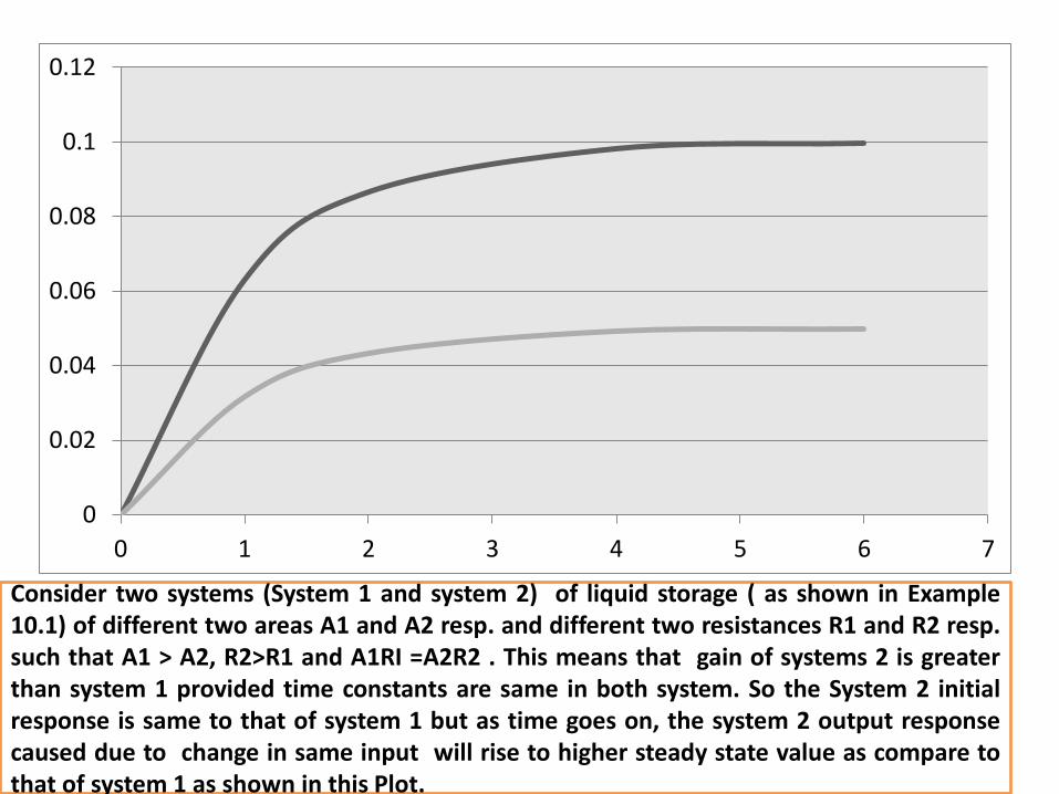
Consider two systems (System 1 and system 2) of liquid storage ( as shown in Example 10.1) of different two areas A1 and A2 resp. and different two resistances R1 and R2 resp. such that A1 > A2, R2>R1 and A1RI =A2R2 . This means that gain of systems 2 is greater than system 1 provided time constants are same in both system. So the System 2 initial response is same to that of system 1 but as time goes on, the system 2 output response caused due to change in same input will rise to higher steady state value as compare to that of system 1 as shown in this Plot.

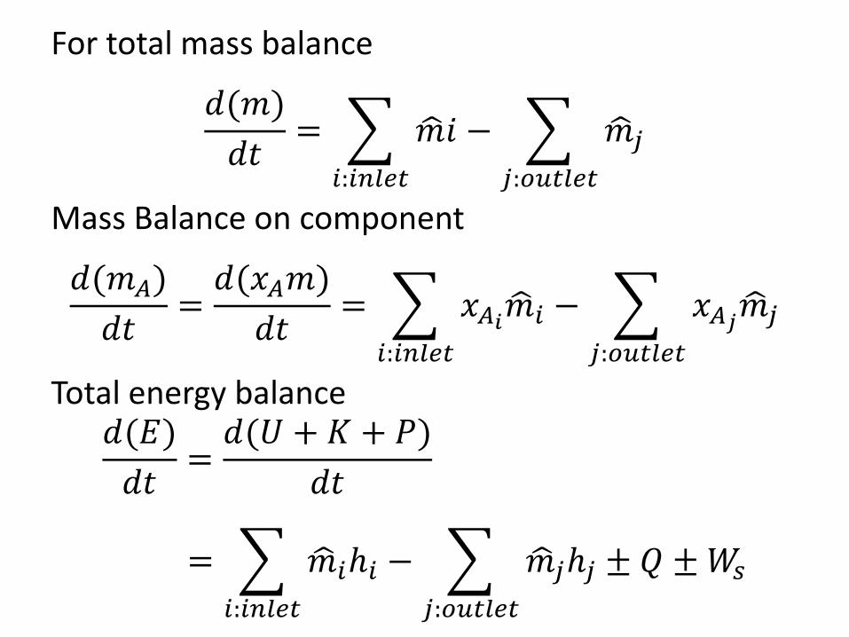
For total mass balance

𝑑(𝑚)

𝑑𝑡= 𝑚 𝑖

𝑖:𝑖𝑛𝑙𝑒𝑡

− 𝑚 𝑗𝑗:𝑜𝑢𝑡𝑙𝑒𝑡

Mass Balance on component

𝑑(𝑚𝐴)

𝑑𝑡=𝑑(𝑥𝐴𝑚)

𝑑𝑡= 𝑥𝐴𝑖𝑚 𝑖

𝑖:𝑖𝑛𝑙𝑒𝑡

− 𝑥𝐴𝑗𝑚 𝑗𝑗:𝑜𝑢𝑡𝑙𝑒𝑡

Total energy balance 𝑑(𝐸)

𝑑𝑡=𝑑(𝑈 + 𝐾 + 𝑃)

𝑑𝑡

= 𝑚 𝑖𝑕𝑖𝑖:𝑖𝑛𝑙𝑒𝑡

− 𝑚 𝑗𝑕𝑗𝑗:𝑜𝑢𝑡𝑙𝑒𝑡

± 𝑄 ±𝑊𝑠

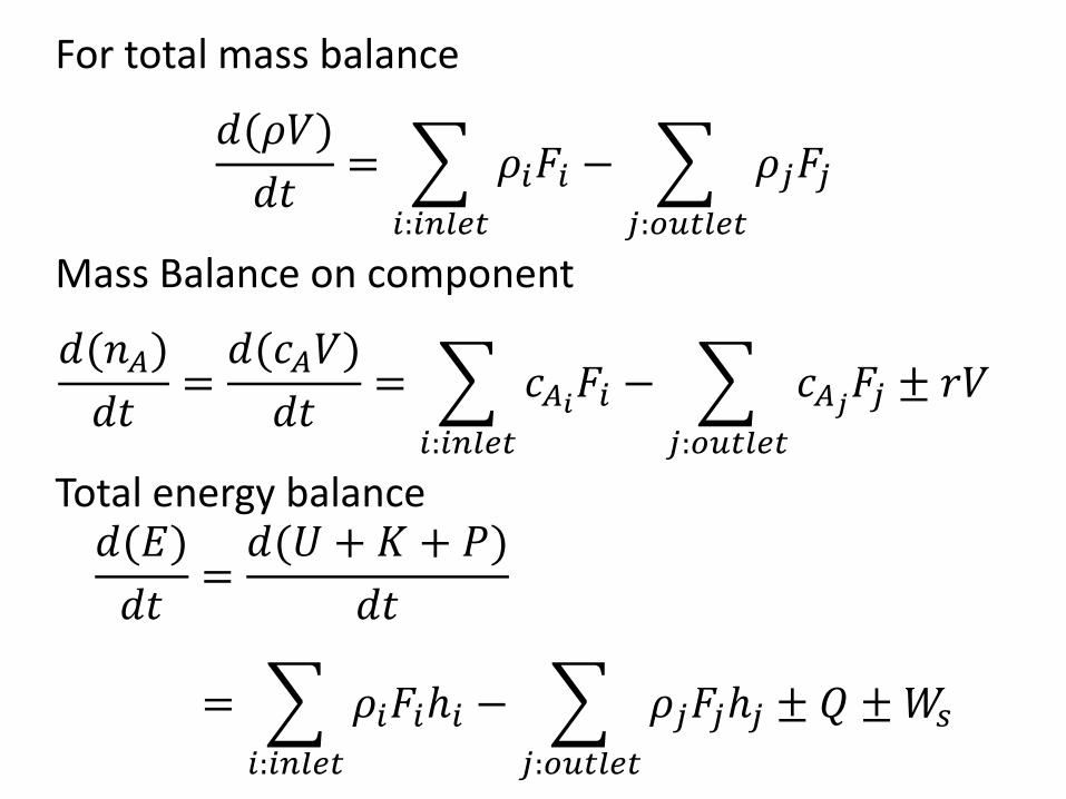
For total mass balance

𝑑(𝜌𝑉)

𝑑𝑡= 𝜌𝑖𝐹𝑖

𝑖:𝑖𝑛𝑙𝑒𝑡

− 𝜌𝑗𝐹𝑗𝑗:𝑜𝑢𝑡𝑙𝑒𝑡

Mass Balance on component

𝑑(𝑛𝐴)

𝑑𝑡=𝑑(𝑐𝐴𝑉)

𝑑𝑡= 𝑐𝐴𝑖𝐹𝑖

𝑖:𝑖𝑛𝑙𝑒𝑡

− 𝑐𝐴𝑗𝐹𝑗𝑗:𝑜𝑢𝑡𝑙𝑒𝑡

± 𝑟𝑉

Total energy balance 𝑑(𝐸)

𝑑𝑡=𝑑(𝑈 + 𝐾 + 𝑃)

𝑑𝑡

= 𝜌𝑖𝐹𝑖𝑕𝑖𝑖:𝑖𝑛𝑙𝑒𝑡

− 𝜌𝑗𝐹𝑗𝑕𝑗𝑗:𝑜𝑢𝑡𝑙𝑒𝑡

± 𝑄 ±𝑊𝑠

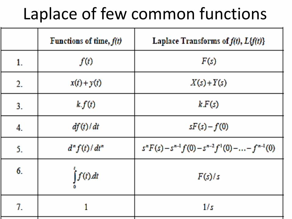
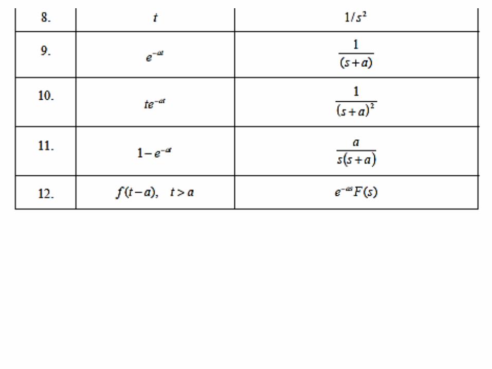
Laplace of few common functions