Basic Probability Theory (基础概率论)

Yaokun Wu (吴耀琨)

东中院 4-106, 2020/03/10

1 Are real numbers real?

In probability theory, we use probability, a number in the unit interval [0, 1] to measure arandom event. So, should we understand real numbers [Sti13] first?

Poincaré maintained that the continuity conditions are warranted and thatphysicists should work with continuous representations of nature, so that dif-ferential calculus is directly applicable, whereas Boltzmann claimed that thecontinuity conditions are problematic, and that physicists should ultimatelytake nature to be discrete, although one can use theories involving differentialequations as idealized models. – [vS15]

Bolzano introduced infinitely great and infinitely small numbers. If hismanuscript were published and recognized by contemporaries, we would haveprobably dealt with another kind of analysis, a nonstandard one. Recall whatPutnam said about the emergence of the epsilon-delta language:“If the epsilon-delta methods had not been discovered, then infinitesimals would have beenpostulated entities (just as‘imaginary’numbers were for a long time). Indeed,this approach to the calculus enlarging the real number system –is just as con-sistent as the standard approach, as we know today from the work of AbrahamRobinson. If the calculus had not been ‘justified’Weierstrass style, it wouldhave been ‘justified’anyway”[Putnam, 1975]. – [Sin15]

1

Peter Bentley2008 写了本英文科普书 The Book of Numbers(数字之书)，南方日报出版社2012 年出版了其中文译本。Mickaël Launay2018 年写了本法文科普书 Le grand roman desmaths(数学的精彩故事)，北京联合出版公司当年出版了其中文译本。两本中文书不约而同地使用了书名《万物皆数》。

All is number （万物皆数）. – Pythagoras of Samos https://nrich.maths.org/2572

Pythagoras and his followers were sure that integers explained everything in life, from natureto music. What’s more, they were sure that everything in the universe was expressible asthe result of rational numbers (ratios of whole numbers).

When we attempt to assert how the universe must be structured, ratherthan attempting to learn how it truly is, we might as well be drown-ing Hippasus ourselves. – https://boxingpythagoras.com/2014/02/26/the-legend-of-hippasus/

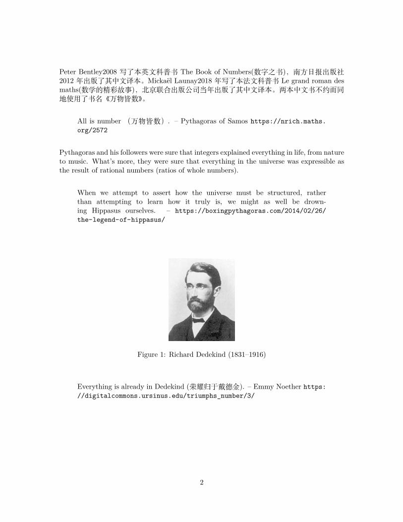
Figure 1: Richard Dedekind (1831–1916)

Everything is already in Dedekind (荣耀归于戴德金). – Emmy Noether https://digitalcommons.ursinus.edu/triumphs_number/3/

2

Richard Dedekind, born in Brunswick on Oct. 6, 1831, did his doctoral work in foursemesters under Gauss’s supervision and submitted a thesis on the theory of Eulerian in-tegrals. He received his doctorate from Göttingen in 1852 and he was to be the last pupilof Gauss. However he was not well trained in advanced mathematics and fully realised thedeficiencies in his mathematical education. Dedekind was a close friend of Bernhard Rie-mann. He taught in Gottingen and Zurich for a while and then returned to his hometownto teach at a local Polytechnikum. He is not interested in offers to move to more prestigousinstitutes.

In 1856, after studying the works of Galois，Dedekind became the first person in the worldto give a lecture on ‘Galois Theory’during his course on mathematics at Gottingen.Dedekind edited the collection of works carried out by Riemann, Dirichlet and Gauss andpublished them in a single volume. In your elementary number theory course, you mayalready see Dedekind’s reciprocity law [RG72]; while in your abstract algebra course, youwill surely see his ideal theory.

Figure 2: Richard Dedekind, Essays on the Theory of Numbers https://www.maa.org/press/periodicals/

convergence/mathematical-treasure-dedekind-on-the-nature-of-number

Although the real numbers were often imagined as points lying on an infiniteline, as a calculus instructor in Zürich, Switzerland, Dedekind became deeplytroubled by the need to reference geometry when teaching his students conceptssuch as functions and limits. This inspired him to develop a rigorous arithmeticfoundation for the set of real numbers, in which, through the use of what are nowcalled ‘Dedekind cuts,’ he cleverly defines both rational and irrational numbers,and demonstrates how they fit together to form the continuum of real numbers.– [Cro16]

3

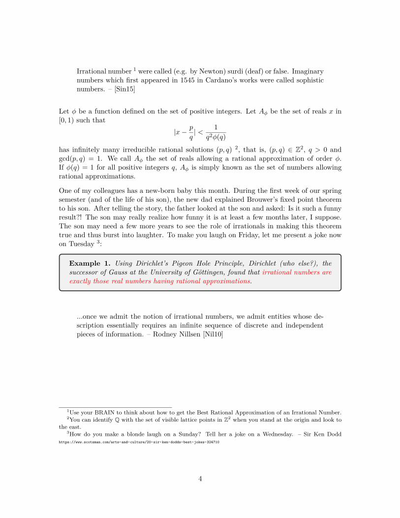
Irrational number 1 were called (e.g. by Newton) surdi (deaf) or false. Imaginarynumbers which first appeared in 1545 in Cardano’s works were called sophisticnumbers. – [Sin15]

Let ϕ be a function defined on the set of positive integers. Let Aϕ be the set of reals x in[0, 1) such that

|x− p

q| < 1

q2ϕ(q)

has infinitely many irreducible rational solutions (p, q) 2, that is, (p, q) ∈ Z2, q > 0 andgcd(p, q) = 1. We call Aϕ the set of reals allowing a rational approximation of order ϕ.If ϕ(q) = 1 for all positive integers q, Aϕ is simply known as the set of numbers allowingrational approximations.

One of my colleagues has a new-born baby this month. During the first week of our springsemester (and of the life of his son), the new dad explained Brouwer’s fixed point theoremto his son. After telling the story, the father looked at the son and asked: Is it such a funnyresult?! The son may really realize how funny it is at least a few months later, I suppose.The son may need a few more years to see the role of irrationals in making this theoremtrue and thus burst into laughter. To make you laugh on Friday, let me present a joke nowon Tuesday 3:

Example 1. Using Dirichlet’s Pigeon Hole Principle, Dirichlet (who else?), thesuccessor of Gauss at the University of Göttingen, found that irrational numbers areexactly those real numbers having rational approximations.

...once we admit the notion of irrational numbers, we admit entities whose de-scription essentially requires an infinite sequence of discrete and independentpieces of information. – Rodney Nillsen [Nil10]

1Use your BRAIN to think about how to get the Best Rational Approximation of an Irrational Number.2You can identify Q with the set of visible lattice points in Z2 when you stand at the origin and look to

the east.3How do you make a blonde laugh on a Sunday? Tell her a joke on a Wednesday. – Sir Ken Dodd

https://www.scotsman.com/arts-and-culture/20-sir-ken-dodds-best-jokes-324710

4

In probability theory, a zero–one law is a result that states that an event must haveprobability 0 or 1 and no intermediate value. 4

To give you an example of such a 0-1 law, we establish a very easy way to measure theprobability of some simple events.

For each interval I, say I = [a, b] or (a, b] or [a, b) or (a, b), its length is |I| = b − a. Ifa set A is a disjoint union of some intervals I1, I2, . . ., it is natural to define its length tobe |A| =

∑k |Ik|. Although taking sum is essentially a finite operation, via the process of

taking limit, we can go to countable summation, which may be divergent or convergent.When you have uncountablely many summands, it looks to be difficult to find a reasonabledefinition of their sum, maybe because our brain/computer is only capable of reading finitewords. In general, if A ⊆ ∪kIk where the countable collection of sets Ik may be disjoint ornot, you should expect |A| ≤

∑k |Ik| whenever you have a way to measure the ‘length’ of

A and those Ik.

For A ⊆ [0, 1), let us say A is negligible 5 if, for every ϵ > 0, there is a countable collectionof intervals I1, I2, . . . such that

A ⊆ ∪kIk,∑k

|Ik| < ϵ.

We want to measure the length of a negligible set A, denoted by |A|. As a length, we shouldhave |A| ≥ 0. Since the length function should respect the inclusion relationship, we shouldhave |A| ≤

∑k |Ik| < ϵ for every ϵ > 0. This says that the only possible choice is to set

|A| = 0.

Note that the length of [0, 1) is 1. For each negligible set A ⊆ [0, 1), let us say that theprobability of a random point in [0, 1) falling into A is P (A) = 0 and the probability of arandom point in [0, 1) falling into Ac=[0, 1) \A is P (Ac) = 1.

Let C0 = [0, 1]. For each positive integer n, let Cn be obtained from Cn−1 by dividing eachinterval of Cn−1 into three intervals of equal length and then removing the middle openinterval from each of the intervals from Cn−1. The Cantor set is defined to be ∩n≥0Cn. Itis one of those famous fractals 6 and has the poetic name of Cantor dust.

Exercise 2. Let C be the Cantor set C. Show that |C| = |R| = |[0, 1]| and P (C) = 0.

4Think of a group of guys who want to visit a bridge. If there is a magic which pushes each guy there toone of the two very endpoints of the bridge, how funny it is!

5青蘋之末, 可忽略的6http://fractals.marguz.net/read/the-nature-of-fractals/

5

For any x ∈ R, if x2 = x then we can conclude that x is either 0 or 1. 7

There are many zero-ones laws in probability theory. Does it mean that the study ofprobability aims to derandomize the randomness?

Theorem 3. • Suppose that ϕ is positive. If∑

q1

qϕ(q) < ∞, then P (Aϕ) = 0.

• Suppose that ϕ is positive and nondecreasing. If∑

q1

qϕ(q) = ∞, then P (Aϕ) = 1. 8

Exercise 4. Verify the first claim in Theorem 3.

Since we know that the set of irrational points in [0, 1) are those points in the intervalhaving rational approximations, the second claim in Theorem 3 confirms that Q ∩ [0, 1) isnegligible – it surely does as it is countable.

Anyone who mindlessly profits from the wonders of science and technology, buthas no more understanding of them than a cow’s appreciation of botany andthe plants that she devours with great pleasure, should be ashamed of himself.– Albert Einstein, opening speech at Berlin Radio exhibit, 1930.

7Remember that, for a set X, X ×X is isomorphic with X if and only if |X| = 0, 1 or ∞.8We will use the continued fraction expansion of a real together with Gauss’s measure to produce a proof

of it when you can really sit in front of our blackboard.

6

2 How many numbers are normal?

Our simple discussion on lengths of some simple sets in the real line was largely extendedin measure theory. A most important one, Lebesgue measure, was presented in the PhDthesis of Henri Léon Lebesgue (1875-1941), instructed by Émile Borel (1871-1956).

In 1894 Lebesgue was accepted at the École Normale Supérieure, where hecontinued to focus his energy on the study of mathematics, graduating in 1897.After graduation he remained at the École Normale Supérieure for two years,working in the library, where he became aware of the research on discontinuitydone at that time by René-Louis Baire, a recent graduate of the school. At thesame time he started his graduate studies at the Sorbonne, where he learnedabout Émile Borel’s work on the incipient measure theory and Camille Jordan’swork on the Jordan measure. In 1899 he moved to a teaching position at theLycée Central in Nancy, while continuing work on his doctorate. In 1902 heearned his Ph.D. with the seminal thesis on “Integral, Length, Area”, submittedwith Borel, four years older, as advisor.

Émile Borel invented the concept of normal number in 1909 [BC18, Bin00, NB77] 9. Usingthe Borel–Cantelli lemma, Borel proved his normal number theorem, also known as thestrong law of large numbers for fair coin tossing 10, which state that almost all real numbersare normal. Let us try to understand what are normal numbers.

Poincaré, knowing everything about everything, knew better than most “that weknow nothing”. – https://www.encyclopediaofmath.org/index.php/Borel,_Émile

Please forget everything you have learned in school; for you haven’t learned it.– Edmund Landau 11

9Many may know bell curve or Gaussian normal distribution. But I hope you agree that normal numbersare no less normal and they are found almost everywhere in your daily life.

10 Pierre-Simon Laplace believes it to be true but cannnot see any proof.11[Sti13, Preface]

7

By now, the concepts Einstein developed on the structure of space and timeshould actually have become a greater part of our cultural heritage; the sameshould be said about some of the consequences his ideas have had on our currentviews of cosmological development. – Harald Fritzsch, The Curvature of Space-time: Newton, Einstein, and Gravitation, Columbia University Press, 2002.

Let us consider numbers in the unit interval Ω = [0, 1), which can be identified with R/Z =S1. Have you ever considered the problem of space and time of this world of the unit circle?12

View the unit interval Ω as our space and throw in a random point. Then it hits on aninterval of length ℓ there with probability ℓ. We can consider more complex subsets there,say unions of a finite set of disjoint intervals or even unions of countably many disjointintervals. The indicator function 1A of such a set A is a step function taking values in0, 1 and having a countablely many discontinuous points. The length of A is the sum ofthe length of its intervals and can be defined as the integral of 1A. That is,

P (A) =

∫Ω

1A(ω)dω =

∫ 1

01A(ω)dω.

Besides assigning probability to those simple sets as above, we have set

P (A) =

0 if A is negligible,1 if Ω \A is negligible.

It is not hard to check that the two definitions does not yield any conflict. When Lebesgueconsidered his measure theory, he tried to measure the length of more subsets of Ω 13. Letus do not go that further at this moment.

12Considering that most nontrivial mathematics is just about Z and R, S1 looks to be a very challengingworld for me.

13You may wonder if there is a way to measure the ‘length’ of every subset A of Ω. I want to know youranswer!

8

A base is an integer greater than or equal to 2. For a real number ω in Ω = [0, 1), theexpansion of ω in base b is a sequence ω1ω2ω3 . . . of integers from 0, 1, . . . , b− 1 such that

ω =∑k≥1

ωkb−k = 0.ω1ω2ω3 . . . .

For any (ω, k) ∈ Ω × N, let d(ω, k) denote the kth digit of ω in its base b expansion, i.e.,d(ω, k) = ωk. Ω is our space and N is our time and we thus come to a map of spacetime.

Fixing k ∈ N, let dk ∈ 0, 1, . . . , b− 1Ω be the map that sends ω to d(ω, k); Fixing ω ∈ Ω,let cω be the expansion of ω in base b, which is a sequence from 0, 1, . . . , b− 1Ω.

The first view of the spacetime gives us a sequence of step functions dk on [0, 1), with thelength of each step of dk being 1

2k. The second view of the spacetime interprets each sample

points ω as a sequence of outcomes of flipping coins. To avoid possible ambuiguity here, letus stick to the base-b expansions which will not end at an infinite string of 0s.

The supports of the step functions dk consists of a finite set of disjoint intervals and so weknow how to measure their lengths and how to integrate dk.

The fact from the time viewpoint that all bn possible outcomes of throwing our b-sided diceare equally possible corresponds to the fact from the space viewpoint that, for any u1 · · ·un,P (ω : dk(ω) = uk, k = 1, . . . , n) = 1

bn .

This world of spacetime is easy to visualize from a rooted b-nary tree: Each node has bchildren which are ordered from leftest to rightest; Two infinite paths originating from theroot are indistinguishable if you can not find a third path inbetween them and the set ofequivalence classes of infinite paths thus obtained correspond to our space Ω; Each dayk ∈ N corresponds to a level/height of the tree.

Our spacetime on Ω is also intrincically related to the self-map on Ω that sends ω to thefractional part of bω.

Or could it happen that the descriptions of the world as a continuum, or as adiscrete (but terribly huge) structure, are equivalent, emphasizing two sides ofthe same reality. – László Lovász [Lov00]

9

For any word w on an alphabet A and any a ∈ A, let |w|a denote the number of occurrencesof a in w. Fix x ∈ Ω = [0, 1).

• We call x simply normal to base b if limn→∞|x1···xn]|d

n = 1b for all d ∈ 0, . . . , b− 1.

• We call x normal to base b if it is simply normal to bases b, b2, b3, .... . Note that thisis equivalent to saying that, for all positive integers n, all n-blocks over 0, 1, . . . , b−1occur in the base-b expansion of x with a limit frequency equal to 1

bn .

• A number is absolutely normal if it is normal to every base.

Exercise 5. Check that this is a number normal to base 10:0.1234567891011121314151617181920212223......

In 1909, Borel showed that the set A of absolutely normal numbers in Ω has a negligiblecomplement, namely P (A) = 1. In 1916, during his time in Moscow, Sierpinski gave thefirst example of an absolutely normal number – Note that Borel showed that almost allreals ω ∈ Ω are absolutely normal but could not give any explicit one. The first computableabsolutely normal number was constructed by Alan Turing in 1936 [Tur36, Tur37, Wel13]. In1950, Borel [Bor50] made the conjecture that all irrational algebraic numbers are absolutelynormal. But, so far we even do not know if

√2 has infinitely-many 5’s [say] in its decimal

expansion [Dub19]!

The game of Heads or Tails, which seems so simple, is characterized by greatgenerality and leads, when studied in details, to the most sophistically mathe-matics. – Émile Borel

10

Figure 3: Sierpiński’s Carpet https://tasks.illustrativemathematics.org/content-standards/tasks/1523

Am I going to be any wiser because of that? – Otto Nikodym (1887–1974),in his response to Sierpiński’s persuasion of taking his doctoral examination.http://mathshistory.st-andrews.ac.uk/Biographies/Nikodym.html

Hopefully, we can go through martingale theory to get an intuitive proof of the Radon-Nikodym theorem [Wil91, §14.13], which is about the derivative or density of a measure λw.r.t. another measure ν, denoted dλ/dν.

11

Let us now count the largeness of the set of normal numbers. On the one hand, we knowthat its complement is very large in the sense that it has the same cardinality with Ω. Onthe other hand, the Strong Law of Large Numbers for coin tossing, also known as Borel’sNormal Number Theorem, says that the set of normal numbers to base 2 has full probability.This is the result:

Theorem 6. The complement of the set of normal numbers to base 2 is uncountable butnegligible.

In probability theory, you can see many different versions of Strong Laws of Large Numbers(SLLN) and Weak Laws of Large Numbers (WLLN). The former is about convergencealmost everywhere (几乎处处收敛) of a sequence of random variables while the latter isabout the convergence in probability (依概率收敛). From their names, you will know thatSLLN implies corresponding WLLN.

Here is the WLLN version of Borel’s Normal Number Theorem. Can you see how to deduceTheorem 7 from Theorem 6?

Theorem 7. For each ϵ > 0, limn→∞ P (ω : |∑n

i=1 di(ω)n − 1

2 | ≥ ϵ) = 0.

12

Borel’s Normal Number Theorem connects time and space: Averaging in time N at almostall ω ∈ Ω produces the same result with averaging in space at every time step k ∈ N, or atheight k of our rooted tree. It is no wonder that this result can be viewed as a special caseof the Birkhoff’s Individual Ergodic Theorem 14.

Birkhoff’s Individual Ergodic Theorem and Von Neumann’s Mean Ergodic Theorem[Moo15], are two classical results of great significance both in mathematics and in statisticalmechanics.

The word ergodic is a mixture of two Greek words: ergon (work) and odos (path). The wordwas introduced by Boltzmann (in statistical mechanics) regarding his hypothesis: for largesystems of interacting particles in equilibrium, the time average along a single trajectoryequals the space average. The hypothesis as it was stated was false, and the investigationfor the conditions under which these two quantities are equal lead to the birth of ergodictheory as is known nowadays.

14See [DK02, §3.1.2] or http://www.stat.yale.edu/~pollard/Courses/600.spring2017/Handouts/Ergodic.pdf.

13

3 In front of a blackboard

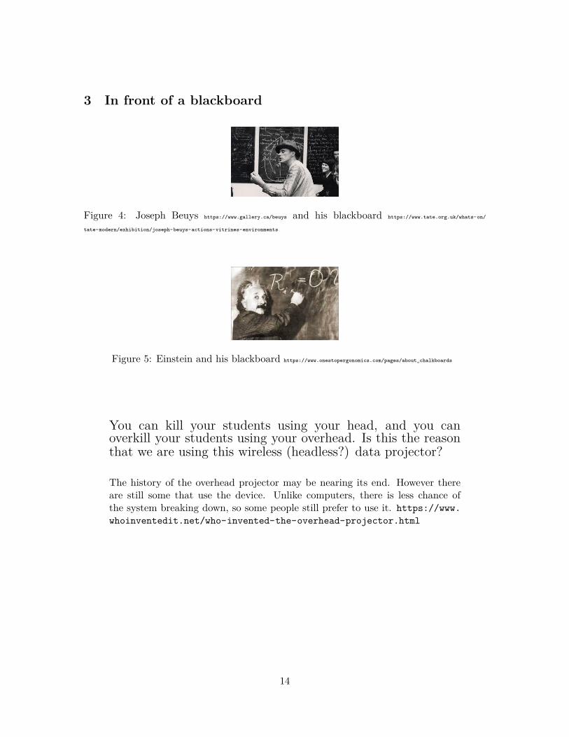
Figure 4: Joseph Beuys https://www.gallery.ca/beuys and his blackboard https://www.tate.org.uk/whats-on/

tate-modern/exhibition/joseph-beuys-actions-vitrines-environments

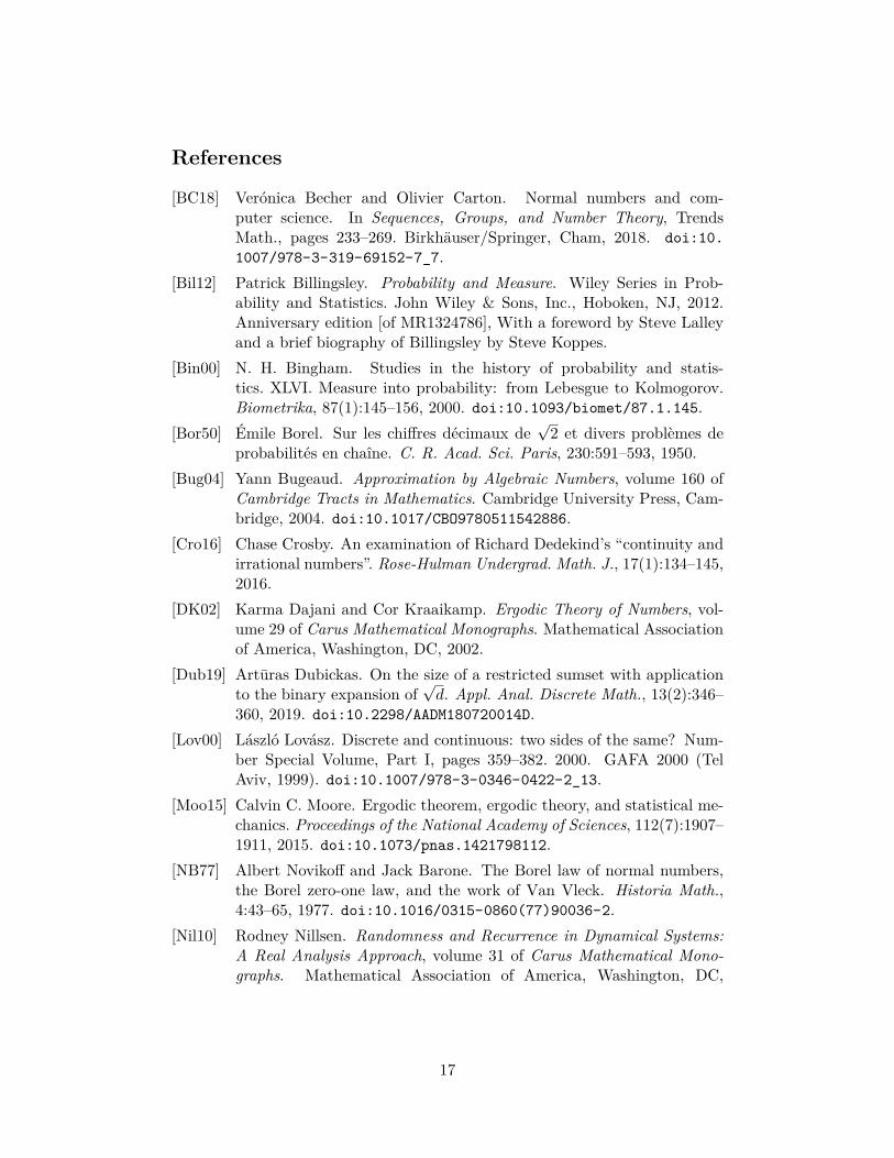
Figure 5: Einstein and his blackboard https://www.onestopergonomics.com/pages/about_chalkboards

You can kill your students using your head, and you canoverkill your students using your overhead. Is this the reasonthat we are using this wireless (headless?) data projector?

The history of the overhead projector may be nearing its end. However thereare still some that use the device. Unlike computers, there is less chance ofthe system breaking down, so some people still prefer to use it. https://www.whoinventedit.net/who-invented-the-overhead-projector.html

14

Let us use our four big blackboards 15 to demonstrate a proof of Example 1and Theorems 6 and 7.

• For any nonnegative simple step functions, we know that its integral isnonnegative. This is the idea behind the so-called Chebyshev’s inequalityand will be used in our proof of Theorems 6 and 7.

• To faciliate our computation in proving Theorems 6 and 7, we will docoordinate transforms to go from the functions dk to functions rk whererk(ω) = 2dk(ω)−1. The nice thing about rk is that they form an orthogonalnormal basis in the linear space generated by them:∫

Ωri(ω)rj(ω)dω = δi,j .

• Let Sn(ω) =∑n

k=1 rk(ω). Check that P (ω : |Sn(ω)| ≥ nϵ) ≤1

n4ϵ4

∫ 10 Sn(ω)

4dω = n+3(n−1)nn4ϵ4

≤ 3n2ϵ4

.• Take a positive decreasing sequence (ϵn)n∈N such that limn→∞ ϵn = 0 and∑

n∈N ϵ−4n n−2 < ∞, say ϵn = n

−18 . Let An = ω : |Sn(ω)

n | ≥ ϵn. We knowthat P (An) ≤ 3

n2ϵ4n.

• Let N ⊆ Ω be the set of normal numbers to base 2. Note that the comple-ment of N is contained in ∩m∈N ∪∞

n=m An = limm→∞ ∪∞n=mAn.

15 https://zuzannamblog.wordpress.com/2017/10/13/drawings/

15

Figure 6: Joseph Beuys (1921-1986), Chalk, blackboard, tray and metal stand http://timelines.

artsy.net/artist/joseph-beuys#9

Figure 7: Four Blackboards in 4-106

Exercise 8. Write down a complete solution to Example 1 and Theorems 6and 7 in a tex file. If necessary, you may consult [Bil12, Chap. 1: Borel’sNormal Number Theorem] for Theorems 6 and 7 and [Bug04, Theorem 1.1] forExample 1 16.

16You can also try http://math.sjtu.edu.cn/faculty/ykwu/data/TeachingMaterial/ENT2.pdf.

16

References

[BC18] Verónica Becher and Olivier Carton. Normal numbers and com-puter science. In Sequences, Groups, and Number Theory, TrendsMath., pages 233–269. Birkhäuser/Springer, Cham, 2018. doi:10.1007/978-3-319-69152-7_7.

[Bil12] Patrick Billingsley. Probability and Measure. Wiley Series in Prob-ability and Statistics. John Wiley & Sons, Inc., Hoboken, NJ, 2012.Anniversary edition [of MR1324786], With a foreword by Steve Lalleyand a brief biography of Billingsley by Steve Koppes.

[Bin00] N. H. Bingham. Studies in the history of probability and statis-tics. XLVI. Measure into probability: from Lebesgue to Kolmogorov.Biometrika, 87(1):145–156, 2000. doi:10.1093/biomet/87.1.145.

[Bor50] Émile Borel. Sur les chiffres décimaux de√2 et divers problèmes de

probabilités en chaîne. C. R. Acad. Sci. Paris, 230:591–593, 1950.[Bug04] Yann Bugeaud. Approximation by Algebraic Numbers, volume 160 of

Cambridge Tracts in Mathematics. Cambridge University Press, Cam-bridge, 2004. doi:10.1017/CBO9780511542886.

[Cro16] Chase Crosby. An examination of Richard Dedekind’s “continuity andirrational numbers”. Rose-Hulman Undergrad. Math. J., 17(1):134–145,2016.

[DK02] Karma Dajani and Cor Kraaikamp. Ergodic Theory of Numbers, vol-ume 29 of Carus Mathematical Monographs. Mathematical Associationof America, Washington, DC, 2002.

[Dub19] Artūras Dubickas. On the size of a restricted sumset with applicationto the binary expansion of

√d. Appl. Anal. Discrete Math., 13(2):346–

360, 2019. doi:10.2298/AADM180720014D.[Lov00] László Lovász. Discrete and continuous: two sides of the same? Num-

ber Special Volume, Part I, pages 359–382. 2000. GAFA 2000 (TelAviv, 1999). doi:10.1007/978-3-0346-0422-2_13.

[Moo15] Calvin C. Moore. Ergodic theorem, ergodic theory, and statistical me-chanics. Proceedings of the National Academy of Sciences, 112(7):1907–1911, 2015. doi:10.1073/pnas.1421798112.

[NB77] Albert Novikoff and Jack Barone. The Borel law of normal numbers,the Borel zero-one law, and the work of Van Vleck. Historia Math.,4:43–65, 1977. doi:10.1016/0315-0860(77)90036-2.

[Nil10] Rodney Nillsen. Randomness and Recurrence in Dynamical Systems:A Real Analysis Approach, volume 31 of Carus Mathematical Mono-graphs. Mathematical Association of America, Washington, DC,

17

2010. With a foreword by Kenneth A. Ross. doi:10.5948/UPO9781614440000.

[RG72] Hans Rademacher and Emil Grosswald. Dedekind Sums. The Mathe-matical Association of America, Washington, D.C., 1972. The CarusMathematical Monographs, No. 16.

[Sin15] Galina Ivanovna Sinkevich. On the history of number line. Antiq.Math., 9:83–92, 2015. doi:10.14708/am.v9i0.832.

[Sti13] John Stillwell. The Real Numbers: An introduction to set theory andanalysis. Undergraduate Texts in Mathematics. Springer, Cham, 2013.doi:10.1007/978-3-319-01577-4.

[Tur36] A. M. Turing. On Computable Numbers, with an Application to theEntscheidungsproblem. Proc. London Math. Soc. (2), 42(3):230–265,1936. doi:10.1112/plms/s2-42.1.230.

[Tur37] A. M. Turing. On Computable Numbers, with an Application to theEntscheidungsproblem. A Correction. Proc. London Math. Soc. (2),43(7):544–546, 1937. doi:10.1112/plms/s2-43.6.544.

[vS15] Marij van Strien. Continuity in nature and in mathematics: Boltzmannand Poincaré. Synthese, 192(10):3275–3295, 2015. doi:10.1007/s11229-015-0701-9.

[Wel13] P. D. Welch. Turing’s mathematical work. In European Congress ofMathematics, pages 763–777. Eur. Math. Soc., Zürich, 2013.

[Wil91] David Williams. Probability with Martingales. Cambridge Math-ematical Textbooks. Cambridge University Press, Cambridge, 1991.doi:10.1017/CBO9780511813658.

18