Tetsuo Sasao and Andre B. FletcherIntroduction to VLBI SystemsChapter 1Lecture Notes for KVN StudentsBased on Ajou University Lecture Notes(to be further edited)Version 2.Issued on February 28, 2005.Revised on March 18, 2005.Revised on February 4, 2006.

Basic Knowledge ofRadio Astronomy

Contents

1 ‘Windows’ for Ground–based Astronomy 3

2 Various Classifications of Astronomical Radio Sources 4

3 Spectra of Typical Continuum Radio Sources 4

4 Spectralline Radio Sources 5

5 Designations of Astronomical Radio Sources 8

6 Designations of Frequency Bands 8

7 Basic Quantities in Radio Astronomy 97.1 Intensity (Specific/Monochromatic Intensity) Iν or Brightness

Bν . . . . . . . . . . . . . . . . . . . . . . . . . . . . . . . . . 97.2 Constancy of the Monochromatic Intensity Iν . . . . . . . . . 107.3 ‘Spectral Flux Density’ or ‘Flux Density’ or ‘Flux’ Sν . . . . . 117.4 Power/Energy/Radiation Flux Density S . . . . . . . . . . . . 127.5 Spectral Energy Density per Unit Solid Angle uν . . . . . . . 127.6 Spectral Energy Density Uν . . . . . . . . . . . . . . . . . . . 13

1

8 Emission and Absorption of Electromagnetic Radiation 138.1 Elementary Quantum Theory of Radiation (A. Einstein, 1916) 138.2 Einstein Coefficients . . . . . . . . . . . . . . . . . . . . . . . 178.3 Number Density of Photons . . . . . . . . . . . . . . . . . . . 17

9 Blackbody Radiation 189.1 Two Extreme Cases of the Planck Spectrum . . . . . . . . . . 209.2 Wien’s Law . . . . . . . . . . . . . . . . . . . . . . . . . . . . 229.3 Spectral Indices of Thermal Continuum Radio Sources . . . . 229.4 Stars are Faint and Gas Clouds are Bright in the Radio Sky . 229.5 Stefan–Boltzmann Law . . . . . . . . . . . . . . . . . . . . . . 249.6 Total Blackbody Radiation from a Star or a Gas Cloud . . . . 249.7 Universality of the Relationship among Einstein’s Coefficients 259.8 Another Important Quantity in Radio Astronomy . . . . . . . 26

10 Radiative Transfer 2610.1 Phenomenological Derivation of the Radiative Transfer Equation 2610.2 Derivation of the Radiative Transfer Equation from Einstein’s

Elementary Quantum Theory of Radiation . . . . . . . . . . . 2710.3 The Simplest Solutions of Radiative Transfer Equation . . . . 2810.4 What is LTE? . . . . . . . . . . . . . . . . . . . . . . . . . . . 3210.5 Spectrum of the Orion Nebula . . . . . . . . . . . . . . . . . . 33

11 Synchrotron Radiation 3411.1 Non–Relativistic Case . . . . . . . . . . . . . . . . . . . . . . 3411.2 Relativistic Case . . . . . . . . . . . . . . . . . . . . . . . . . 36

2

1 ‘Windows’ for Ground–based Astronomy

Figure 1 shows how the Earth’s atmosphere transmits electromagnetic wavesfrom the Universe. The curve over the hatched area in this figure correspondsto the height in the atmosphere at which the radiation is attenuated by afactor of 1/2.

Figure 1: ‘Windows’ for ground-based astronomy (from Rohlfs & Wilson,2001).

This figure shows that the Earth’s atmosphere is largely transparent inthe radio (15 MHz – 300 GHz) and visible light (360 THz – 830 THz) regionsof the electromagnetic spectrum. These two regions are the main ‘windows’for ground-based astronomical observations. VLBI (Very Long Baseline In-terferometry) is one of the techniques used to observe astronomical radiosources through the ‘radio window’.

3

2 Various Classifications of Astronomical Ra-

dio Sources

There are several ways to classify astronomical radio sources. Typical clas-sifications are:

• – Thermal sourceSource emitting via a thermal mechanism (e.g. blackbody radia-tion),

– Non-thermal sourceSource emitting via a non-thermal mechanism (e.g. synchrotronradiation, inverse Compton scattering, annihilation radiation, maseremission, etc.),

• – Continuum sourceSource emitting over a broad range of frequencies,

– Spectralline sourceSource emitting in narrow lines at specific frequencies,

and

• – Galactic sourceSource inside our Milky Way Galaxy,

– Extragalactic sourceSource outside our Galaxy.

3 Spectra of Typical Continuum Radio Sources

Figure 2 shows typical spectra of continuum radio sources.These spectra are characterized by a quantity called ‘spectral index’ α, de-fined by the formula: Sν ∝ ν−α, where Sν is a quantity called the ‘fluxdensity’ [unit: Jy (Jansky) ≡ 10−26Wm−2Hz−1], which is a measure of thestrength of the radiation from a source.

Thermal and non–thermal sources usually show different spectral indices,namely:

α ∼= −2 for thermal sources,and

α ≥ 0 for non-thermal sources.

4

Figure 2: Spectra of galactic and extragalactic continuum radio sources (fromKraus, 1986).

4 Spectralline Radio Sources

An example of a thermal spectralline source showing many molecular linesis given in Figure 3.

Examples of spectra of non-thermal maser line sources obtained in testobservations for the VERA (VLBI Exploration of Radio Astrometry) arrayin Japan are shown in Figures 4, 5, and 6.

5

Figure 3: Thermal molecular lines observed in the Orion-KL star–formingregion (Kaifu et al., 1985).

Figure 4: H2O maser lines in Cep A (left), and RT Vir (right) (courtesy ofVERA group, Japan, 2002).

6

Figure 5: SiO maser lines in Orion-KL (left), and R Cas (right) observed inpointing tests for a VERA antenna (courtesy of VERA group, Japan, 2002).

Figure 6: H2O maser lines in W49 N and OH43.8, observed simultaneouslywith a VERA dual-beam antenna (courtesy of VERA group, Japan, 2002).

7

5 Designations of Astronomical Radio Sources

There are many designation systems for naming radio sources. Examplesare given in the following. As a result, radio sources are often identified byseveral different names.

• IAU 1974 system of designation (‘IAU name’, see, e.g., ExplanatorySupplement to American Astronomical Almanac)

– identifies a radio source by a six, seven, or eight-digit number,such as 0134+329, which tells us that the right ascension of thesource is 01h 34m, and its declination is +32.9 (usually in theB1950 equinox system).

– sometimes source types or catalog acronyms are added, e.g., pul-sars are called ‘PSR0950+08’, and sources from the Parkes SkySurvey as ‘PKS1322-42’.

• 3C-name, 4C-name

– identifies an extragalactic radio source by a serial number in theThird Cambridge Catalog, and by declination in the Fourth Cam-bridge Survey Catalog.

– examples are 3C84, 3C273, 3C345, 4C39.25, etc.

• W-name

– is based on Westerhout’s (1958) catalog of HII regions.

– examples are W49 N, W3(OH), W51 M, etc.

6 Designations of Frequency Bands

The basic unit of radio frequency is Hz (Hertz: cycle per second). In orderto describe high frequency, typically used in radio astronomical observationsor communications, we frequently use the following secondary units: kHz(kilohertz: 103 Hz), MHz (megahertz: 106 Hz), GHz (gigahertz: 109 Hz),and THz (terahertz: 1012 Hz).

Radio frequency bands used in astronomical observations, as well as incommunications, are designated by one or a few alphabetic characters. Twosystems of designations are shown in Figure 7.

In radio astronomy, IEEE STD-521-1976 designations have been used.Examples are:

8

Figure 7: Frequency designations.

• L–band : GPS satellite, observations of OH masers,

• S– and X–bands : geodetic VLBI observations,

• K–band : observations of H2O masers, and

• Q–band : observations of SiO masers.

7 Basic Quantities in Radio Astronomy

The following quantities are commonly used in radio astronomy to charac-terize radio waves coming from celestial bodies.

7.1 Intensity (Specific/Monochromatic Intensity) Iν or

Brightness Bν

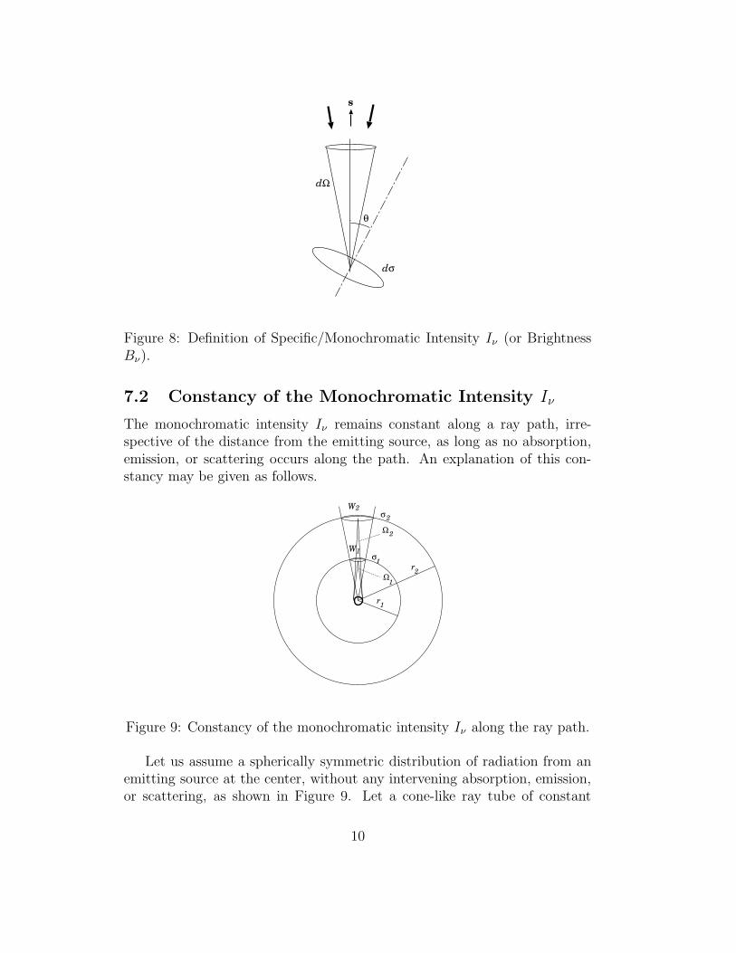
The intensity Iν (or brightness Bν) is the quantity of electromagnetic radia-tion energy incoming from a certain direction in the sky, per unit solid angle,per unit time, per unit area perpendicular to this direction, and per unitfrequency bandwidth with center frequency ν. The SI unit of this specific(or monochromatic) intensity is thus: W m−2 Hz−1 sr−1 (Figure 8).

In terms of the monochromatic intensity Iν , the power dW of radiationcoming from a direction s within a solid angle dΩ, through a cross-section ofarea dσ with a normal inclined by an angle θ from the direction s, within afrequency bandwidth dν centered at ν, is given by:

dW = Iν(s) cos θ dΩ dσ dν. (1)

9

s

θ

dΩ

dσ

Figure 8: Definition of Specific/Monochromatic Intensity Iν (or BrightnessBν).

7.2 Constancy of the Monochromatic Intensity Iν

The monochromatic intensity Iν remains constant along a ray path, irre-spective of the distance from the emitting source, as long as no absorption,emission, or scattering occurs along the path. An explanation of this con-stancy may be given as follows.

W

W

σ

σ

Ω

Ωr

r

11

2

2

12

1

2

Figure 9: Constancy of the monochromatic intensity Iν along the ray path.

Let us assume a spherically symmetric distribution of radiation from anemitting source at the center, without any intervening absorption, emission,or scattering, as shown in Figure 9. Let a cone-like ray tube of constant

10

opening angle intersect a sphere of radius r, forming a cross–section of areaσ, and let the source be seen to subtend a solid angle Ω at this radius. Thepower of the radiation with bandwidth ∆ν passing through this cross–sectionis W = Iν Ω σ∆ν, which must be constant at any radius along the tube, aslong as the radius is much larger than the source size. Now, the solid angle ofthe source Ω and the area of the cross–section σ vary as Ω ∝ r−2 and σ ∝ r2,respectively. Therefore, the monochromatic intensity Iν = W/(Ω σ ∆ν)must be constant along the path.

7.3 ‘Spectral Flux Density’ or ‘Flux Density’ or ‘Flux’

Sν

The spectral flux density Sν is the quantity of radiation energy incomingthrough a cross section of unit area, per unit frequency bandwidth, andper unit time. A special unit called ‘Jansky (Jy)’ is widely used in radioastronomy for the spectral flux density. This unit is defined as: 1 Jy = 10−26

W m−2 Hz−1.

s

θ

∆σ

Figure 10: Definition of spectral flux density Sν.

The spectral flux density Sν is related to the intensity Iν by an integralover a solid angle Ω:

Sν =∫∫

Ω

Iν(s) cos θ dΩ,

=∫∫

Ω

Iν(θ, φ) cos θ sin θ dθ dφ, (2)

11

where Ω could be, for example, a solid angle subtended by a radio source(see Figure 10).

7.4 Power/Energy/Radiation Flux Density S

The power/energy/radiation flux density S is the quantity of radiation en-ergy, over the whole frequency range, incoming through a cross section ofunit area, per unit time. Therefore,

S =

∞∫

0

Sν dν. (3)

When we are interested in the “received” power flux density only, werestrict the range of integration to the observing bandwidth ∆ν, i.e.,

S =∫

∆ν

Sν dν. (4)

The unit of power flux density is: W m−2.

7.5 Spectral Energy Density per Unit Solid Angle uν

The spectral energy density per unit solid angle, uν(s), is the volume densityof the radiation energy incident from a certain direction s, per unit solidangle, and per unit frequency bandwidth. The unit is J m−3 Hz−1 sr−1.

c dt

ds

σ

Figure 11: Radiation energy per unit solid angle in a tube.

Let us consider a cylindrical tube with a cross section of area dσ perpen-dicular to the ray propagation direction, and with a length cdt, which is thedistance travelled by the radiation during a time interval dt at light speed c( = 2.998 × 108 m s−1) (see Figure 11). The radiation energy dUν (J Hz−1

sr−1) per unit solid angle, and per unit frequency bandwidth, contained inthe cylinder may be expressed either in terms of the spectral energy densityper unit solid angle, uν(s), or in terms of the intensity Iν(s), as:

dUν = uν(s) cdt dσ,

dUν = Iν(s) dt dσ. (5)

12

Therefore, these quantities are related to each other by:

Iν(s) = c uν(s). (6)

7.6 Spectral Energy Density Uν

The spectral energy density Uν is the volume density of the energy of theradiation, per unit frequency bandwidth, incoming from all directions (Figure12).

Figure 12: Spectral energy density: energy of radiation coming from alldirections, contained in a unit volume.

Therefore,

Uν =∮

uν(s)dΩ =1

c

∮

Iν(s)dΩ. (7)

The unit is J m−3 Hz−1.

8 Emission and Absorption of Electromag-

netic Radiation

8.1 Elementary Quantum Theory of Radiation (A. Ein-

stein, 1916)

Let us consider a gaseous medium consisting of a large number of particles(atoms or molecules) of the same species. Let us also consider that eachparticle exists in one of the quantum states Z1, Z2, ..., with energy levelsE1, E2, ... . If Em < En for a pair of states Zm and Zn, a particle canabsorb an amount of radiation energy En − Em in a transition from Zm toZn. Also, a particle can emit the same amount of energy in a transition from

13

Zn to Zm (Figure 13). The frequency of the absorbed or emitted radiationis determined by the equation:

hνmn = En − Em, (8)

where h is the Planck constant (h = 6.626 × 10−34 J s).

Z m

E=EnZ n

Z 3Z 2Z 1

E=Em

E=E3E=E2E=E1

hνmn=En-Em hνmn=En-Em

Figure 13: Energy levels and transitions with emission (left–hand arrow) orabsorption (right–hand arrow) of radiation.

The energy levels here may be distributed continuously (continuum emis-sion) or discretely (line emission). Note that even in the discrete level case,the frequency is spread over a finite ‘line width’, due to the Doppler shifts inrandomly moving gaseous media in the universe.

Three kinds of transitions may occur between these two states (Figure14), as follows:

(1) Spontaneous emission Zn → Zm

The spontaneous emission emerges due to a transition which occurs ‘byitself’, without any external influence (Figure 15). The probability dfsp forthe spontaneous emission to occur within a small solid angle dΩ towards adirection -s, within a small frequency bandwidth dν around the frequencyνmn = (En − Em) / h, and during a small time interval dt, must be propor-tional to dν dΩ dt. Therefore, the probability can be expressed through a

14

Z

Z

n

mSpontaneous Emission Absorption Induced Emission

E=En

E=Em

Figure 14: The three possible transitions between two energy states.

certain coefficient αmn as:

dfsp = αmn dν dΩ dt. (9)

-sdΩ

En

Em

E=

E=

Figure 15: Spontaneous emission of radiation.

(2) Absorption Zm → Zn

Some of the radiation passing through the gaseous medium may be ab-sorbed in a transition from Zm to Zn, at a frequency around νmn = (En −Em) / h (Figure 16). The absorption probability dfab for the radiation inci-dent from a direction within a small solid angle dΩ around s, and in a smallfrequency bandwidth dν, during a short time interval dt, must be propor-tional to dν dΩ dt and to the spectral energy density per unit solid angle,uν(s), of the radiation itself. Therefore, introducing a proportionality coeffi-cient βn

m, we have:dfab = βn

m uν(s) dν dΩ dt. (10)

(3) Induced (or stimulated) emission Zn → Zm

Radiation with a frequency ν incident from a certain direction s mayinduce (or ‘stimulate’) transitions of gas particles from higher to lower energy

15

dΩ s

u (s)ν

En

Em

E=

E=

Figure 16: Absorption of radiation.

levels, such that the newly emitted radiation has the same frequency ν, andthe same direction of propagation -s, as the incident radiation (Figure 17).The probability dfst for the induced (or stimulated) emission to occur in a

dΩ s

u (s)νEm

EnE=

E=

Figure 17: Induced (or stimulated) emission of radiation.

direction within a small solid angle dΩ around -s, and in a small frequencybandwidth dν around νmn = (En − Em) / h, during a short time intervaldt, must be proportional to dν dΩ dt and to the spectral energy density perunit solid angle uν(s) of the incident radiation. Therefore, introducing aproportionality coefficient βm

n , we have:

dfst = βmn uν(s) dν dΩ dt. (11)

16

8.2 Einstein Coefficients

The three coefficients αmn , βn

m, and βmn , describing the probabilities of the

three possible transitions:

dfsp = αmn dν dΩ dt,

dfab = βnm uν(s) dν dΩ dt,

dfst = βmn uν(s) dν dΩ dt, (12)

are called the “Differential Einstein Coefficients”. They are usually isotropic,i.e. they do not depend on the direction of propagation of radiation.

Einstein originally described the transition probabilities in the followingform, for the case of an isotropic radiation field, and with the particles atrest:

dWsp = Amn dt,

dWab = BnmUν dt,

dWst = Bmn Uν dt, (13)

where Uν =∮

uν(s) dΩ is the spectral energy density (in units of J m−3 Hz−1).The coefficients Am

n , Bnm, and Bm

n , are called the “Einstein Coefficients”. Insuch a case, the spectral lines due to the transitions between discrete energylevels must be monochromatic lines having no Doppler broadening, since theparticles are at rest. If we introduce f(ν) as the probability distribution offrequency within a spectral line in a real interstellar medium in motion, thetwo sets of coefficients are related to each other, as follows:

αmn =

Amn f(ν)

4π,

βnm = Bn

m f(ν),

βmn = Bm

n f(ν). (14)

8.3 Number Density of Photons

Let the number densities of particles (number of particles per unit volume) inthe states Zm and Zn be nm and nn, respectively. Then the number density ofphotons emitted by the Zn → Zm transition into the solid angle dΩ aroundthe direction -s, within the bandwidth dν, during the time interval dt, isequal to:

nn(dfsp + dfst) = nn(αmn + βm

n uν) dν dΩ dt.

17

Z E

Z E

n

n

n

m

n

m

n

m

Figure 18: Number densities of particles in the two energy states.

On the other hand, the number density of photons in the same solid angledΩ, and the same bandwidth dν, absorbed by the Zm → Zn transition duringthe time interval dt, is equal to:

nmdfab = nmβnmuν dν dΩ dt.

The differential changes in the number density of photons per unit solidangle around -s, and per unit bandwidth around νmn = (En −Em)/h, in thecourse of the absorption and emission is now given by:

dnp(s, ν) dν dΩ = −nmβnmuν + nn [αm

n + βmn uν(s)]dν dΩ dt.

Therefore, the time variation of the number density of photons is describedby the following equation (Figure 19):

dnp(s, ν)

dt= (nnβm

n − nmβnm)uν(s) + nnαm

n . (15)

n

n

n

m

s dΩ

n (s, ν) at t n (s, ν) at t + dtp p

Figure 19: Time variation of the number density of photons.

9 Blackbody Radiation

We now consider the case when the radiation and matter are in thermody-namic equilibrium. Then, we have the following:

18

1. Stationary conditions:The number of transitions Zm → Zn must be equal to the number ofopposite transitions Zn → Zm. Requiring this stationarity in equation(15), we have:

nmβnmuν(s) = nn[αm

n + βmn uν(s)]. (16)

2. Boltzmann distribution:The probability Pn for a particle to be in a state Zn, with energy levelEn, is given by the formula:

Pn = gne−

EnkT , (17)

where k = 1.381 × 10−23 J K−1 is the Boltzmann constant, T is theabsolute temperature of the medium in Kelvin (K), and gn is the sta-tistical weight (reflecting in particular the degree of degeneracy) of thestate Zn.

If we denote the number density of all particles as n, the ratio nn/n mustbe equal to the probability Pn (at least in the statistical sense). Therefore,we have

nm

n= gme−

EmkT , (18)

andnn

n= gne−

EnkT . (19)

Inserting equations (18) and (19) into equation (16), we obtain

e−EmkT gmβn

muν(s) = e−EnkT gn[αm

n + βmn uν(s)]. (20)

Einstein discussed the implications of this equation, as follows:

1. The energy density per unit solid angle of the thermal radiation musttend to infinity (uν(s) → ∞) when the temperature of the mediumtends to infinity (T → ∞) in equation (20). Hence, we obtain

gmβnm = gnβm

n . (21)

Consequently, equation (20) becomes

(eEn−Em

kT − 1)βmn uν(s) = αm

n . (22)

If we take into account the relation hν = En−Em (hereafter, we denoteνmn = ν for simplicity), the energy density per unit solid angle can beexpressed as

uν =αm

n

βmn

1

ehνkT − 1

. (23)

19

Henceforth, we omit the s dependence in uν, since the RHS of equation(23) does not depend on any specific direction, as expected from theisotropic nature of thermal radiation.

2. The energy density per unit solid angle uν must follow the well-knownRayleigh–Jeans radiation law:

uν =2ν2

c3kT, (24)

in the classical limit hν kT . Therefore, we must require in equation(23)

αmn

βmn

=2hν3

c3. (25)

The above discussions thus lead to Planck’s formula of blackbody radiation:

uν =2hν3

c3

1

ehνkT − 1

. (26)

For the intensity Iν , we obtain

Iν = cuν =2hν3

c2

1

ehνkT − 1

, (27)

(see Figure 20). For the energy density Uν , we have

Uν =∮

uνdΩ = 4πuν =8πhν3

c3

1

ehνkT − 1

. (28)

9.1 Two Extreme Cases of the Planck Spectrum

• Rayleigh–Jeans region (hν kT , and hence ehνkT ' 1 + hν

kT):

Iν =2ν2

c2kT. (29)

Note that thermal radiation in the radio frequency range is mostly inthe Rayleigh–Jeans region.

• Wien region (hν kT ):

Iν =2hν3

c2e−

hνkT . (30)

20

104 106 108 1010 1012 1014 1016 1018 1020 102210−25

10−20

10−15

10−10

10−5

1

105

1010

1015104 102 1 10−2 10−4 10−6 10−8 10−10 10−12 10−14

Inte

nsity

I ν (W

Hz−1

m−2

rad−2

)

Frequency ν (Hz)

Wavelength λ (m)

T=1K 10K 102K 103K 104K 105K106K107K 108K109K1010K

Figure 20: Planck spectrum of black body radiation. Each curve correspondsto a certain absolute thermodynamic temperature value.

21

9.2 Wien’s Law

The peak frequency of the Planck spectrum at a given temperature T is

νmax (in Hz) = 5.8789 × 1010T (in K). (31)

One can easily derive this law by equating to zero the derivative of theintensity Iν with respect to frequency ν, in equation (27).

This, Wien’s law, explains why stars with higher temperatures appearbluer, and those with lower temperatures appear redder. Conversely, as-tronomers infer one of the most important physical parameters of stars, thesurface temperature, from measuring their color.

Can we observe the peak of the thermal blackbody spectrum inthe radio region?

• No hope for thermal radiation from a stellar surface, or from a fairlywarm interstellar cloud.

• For submillimeter waves at around 500 GHz (which are still regardedas radio waves), we can see the peak if the temperature of the mediumis below 10 K (T ≤ 10 K).

• For example, the cosmic background radiation with T ' 2.7 K has itspeak at around 170 GHz.

9.3 Spectral Indices of Thermal Continuum Radio Sources

We now understand why the spetral indicies α (Sν ∝ ν−α) of thermal contin-uum radio sources like the Moon, the quiet Sun, and the left half portion ofthe spectrum of Orion nebula, are all close to −2 (α ' −2). This is becausethermal continuum sources mostly show Rayleigh–Jeans spectra, Iν = 2ν2

c2kT ,

in the radio region.

9.4 Stars are Faint and Gas Clouds are Bright in the

Radio Sky

According to the Planck spectrum, the intensity of a hotter black body isalways stronger than the intensity of a colder body, for any frequency range.On the other hand, the flux density Sν, which we directly detect with ourradio telescopes, is proportional to the product of the intensity Iν and thesolid angle of the radio source Ω (Sν ∝ IνΩ). While the surface temperatures

22

Figure 21: Spectra of continuum radio sources (Kraus, 1986; left), and anoptical image of the Moon (right). Do we see such a halfmoon image in radiowaves?

23

of ordinary stars are fairly high (several thousands to several tens of thousandKelvin), their solid angles, which are inversely proportional to their squareddistances, are very small. For example, if we were to put the Sun at thedistance of the nearest star, which is about 3 light years, or 1 parsec, theSun’s angular diameter would be only ' 0.01 arcsecond! As a result, theflux density 5 × 106 Jy of the quiet Sun at 10 GHz (see Figure 2) would bereduced down to 125 µJy at the distance of the nearest star. On the contrary,the interstellar gas clouds, as cold as tens to hundreds of Kelvin, still clearlyshine in the radio sky, because their angular diameters are as large as minutesto degrees of arc. For example, Figure 2 shows that the flux density of theOrion Nebula is about 500 Jy at around 500 MHz.

9.5 Stefan–Boltzmann Law

The total intensity I(T ) of the thermal radiation from a black body of tem-perature T , over the entire frequency range, is given by

I(T ) =

∞∫

0

Iνdν =

∞∫

0

2hν3

c2

1

ehνkT − 1

dν =1

πσT 4, (32)

where σ is the Stefan–Boltzmann constant:

σ =2π5k4

15c2h3= 5.6697 × 10−8 W m−2 K−4.

Equation (32) can be derived using the integration formula:∞∫

0

2x2n−1

e2πx − 1dx =

Bn

2n, (33)

where Bn is the n-th Bernoulli number, and B2 = 1/30.

9.6 Total Blackbody Radiation from a Star or a Gas

Cloud

The power flux density S?, at a surface of a blackbody, which is the powerover the entire frequency range through a cross section of unit area of thesurface (Figure 22), is given by the equation:

S? =

∞∫

0

Sν dν =

∞∫

0

π2

∫

0

2π∫

0

Iν cos θ sin θ dφ dθ dν

= I(T )

π2

∫

0

2π∫

0

cos θ sin θ dφ dθ = π I(T ) = σT 4. (34)

24

θφ

Figure 22: Thermal radiation from a surface of a black body.

Therefore, the total power F of the blackbody radiation from a sphericalstar with radius R is equal to:

F = 4πR2S? = 4πR2σT 4.

The power flux density of the thermal radiation which we receive from a staror a cloud of solid angle Ω, surface temperature T , and distance r, is fromequation (32):

S = Ω I =ΩσT 4

π,

which, for the spherically symmetric case where Ω = πR2/r2, is reduced to

S =R2

r2σT 4 =

R2

r2S? =

F

4πr2,

as expected.

9.7 Universality of the Relationship among Einstein’sCoefficients

We derived equations (21) and (25), giving the following relationships amongEinstein’s coefficients:

gmβnm = gnβm

n ,

αmn

βmn

=2hν3

c3,

or, equivalently,

gmBnm = gnBm

n ,

Amn

Bmn

=8πhν3

c3,

25

by assuming thermodynamic equilibrium. However, the resulting equationsabove do not contain any quantity characteristic of thermodynamics. Thismeans that the equations must hold universally, irrespective of whether thecondition of thermodynamic equilibrium is fulfilled. These relationships aredetermined by the microscopic interactions between a photon and a particle,and are not influenced by the environment (temperature, pressure, ... etc.).We obtained the relationships under the assumption of thermodynamic equi-librium, where it is most easily derived. Analogously, if you find a big holein a road in daytime, you would assume that the hole still exists at night,when you cannot see it well.

9.8 Another Important Quantity in Radio Astronomy

Brightness TemperatureThe brightness temperature TB of a source with monochromatic intensity

(or surface brightness) Iν , is a quantity which is defined by the equation:

TB =c2

2kν2Iν. (35)

This is a quantity with the dimension of temperature obtained by a ‘forced’application of the Rayleigh–Jeans formula to the radiation from any radiosource. If the radiation comes from a sufficiently hot (T 10 K) thermalsource, without noticeable absorption or additional emission along the prop-agation path, the brightness temperature must correspond to the physicaltemperature of the source. If the source is non–thermal, the brightness tem-perature has no relevance to any real temperature. For example, for somemaser sources, the brightness temperature could be as high as 1014 K, al-though the physical temperature values of the ‘masing’ (i.e. maser–emitting)gas clouds are only several hundreds of Kelvin. The word ‘brightness tem-perature’ is a jargon term which is used only, but quite frequently, in radioastronomy.

10 Radiative Transfer

10.1 Phenomenological Derivation of the Radiative Trans-

fer Equation

Radiative transfer theory describes how the intensity varies as radiation prop-agates in an absorbing and/or emitting medium. The equation of radiativetransfer can be phenomenologically derived as follows:

26

Let the intensity Iν change by dIν due to absorption and emission asthe radiation passes through an infinitesimal distance dl (Figure 23). The

s

dl

I (s, l) I (s, l + dl)ν ν

Figure 23: Radiative transfer through a cylinder of infinitesimal length.

variation can be described as a sum of two contributions: one due to theabsorption −κνIνdl, and one due to the emission ενdl, where κν and εν arethe following frequency–dependent coefficients:

κν : opacity m−1,εν : emissivity W m−3 Hz−1 sr−1.

We then obtain the radiative transfer equation in the following form:

dIν

dl= −κνIν + εν . (36)

10.2 Derivation of the Radiative Transfer Equation fromEinstein’s Elementary Quantum Theory of Radi-

ation

Equation (36) can also be derived from equation (15) obtained in the discus-sion of Einstein’s elementary quantum theory of radiation:

dnp(s, ν)

dt= (nnβm

n − nmβnm)uν(s) + nnαm

n ,

where np is the number density of photons per unit solid angle and per unitfrequency bandwidth, uν is the spectral energy density per unit solid angle,nm and nn are the number densities of the particles in states Zm and Zn,and αm

n , βmn and βn

m are Einstein’s differential coefficients. In fact, using therelations:

uν(s) = hνnp(s, ν),

Iν(s) = cuν(s),

dl = cdt ,

we can transform equation (15) to:

dIν

dl= −(nmβn

m − nnβmn )

hν

cIν + hνnnαm

n . (37)

27

Therefore, if we denote

κν = (nmβnm − nnβm

n )hνc

: absorption and induced emission,εν = hνnnαm

n : spontaneous emission,(38)

equation (37) is reduced to the radiative transfer equation (36).

Role of the induced emissionIn the resulting radiative transfer equation:

dIν

dl= −κνIν + εν ,

the opacity κν now contains not only the contribution of simple absorptionbut also that of induced emission, as we see in equation (38). According toequation (21) obtained by Einstein:

gmβnm = gnβm

n ,

we can now express the opacity κν as

κν = (nm −gm

gnnn)βn

m

hν

c. (39)

If we consider the simple case where the statistical weights of the two statesare equal to each other (gm = gn), the above equation (39) reduces to

κν = (nm − nn)βnm

hν

c. (40)

It is worthy to note that the opacity takes on a negative value when thenumber density of the particles in the higher energy level is larger than thatat the lower level (nn > nm).

10.3 The Simplest Solutions of Radiative Transfer Equa-tion

Let us solve the radiative transfer equation (36):

dIν

dl= −κνIν + εν ,

under the following simple conditions.

28

1. When κν = 0,the solution of equation (36) is just a simple integral:

Iν(l) = Iν(0) +

l∫

0

εν(l′)dl′ . (41)

2. When εν = 0,the solution is an exponential function:

Iν(l) = Iν(0)e−

l∫

0

κν(l′)dl′

. (42)

If the medium is homogeneous, i.e. κν = constant everywhere, then

Iν(l) = Iν(0)e−κν l . (43)

Here,κν > 0 (positive opacity) implies an exponential decay, which arisesfrom ordinary absorption, andκν < 0 (negative opacity) implies an exponential growth, which arisesfrom maser amplification.

Maser Amplification

When the number density nn of particles at a higher energy level En

is, for some reason, larger than nm at a lower energy level Em (sucha situation is called a “population inversion”), the opacity becomesnegative (κν < 0), and the radiation of the frequency corresponding tothe transition between the energy levels is exponentially amplified alongthe initial direction of propagation (Figure 24). Since this amplificationis due to induced (or stimulated) emission, it is called a “MASER”(Microwave Amplification of Stimulated Emission of Radiation). Thesame mechanism in the visible light region of electromagnetic wavesis called the “LASER” (Light Amplification of Stimulated Emission ofRadiation).

If the thermal equilibrium condition is fulfilled in the gas medium, theBoltzmann distribution always ensures nn < nm, and no maser amplifi-cation can occur. Therefore, maser emission is essentially non–thermal.We need some “pumping mechanism” which realizes the population in-version in order to get the maser mechanism to work. In actual inter-stellar space, strong infrared radiation from stars, or collisions of gasmolecules, may serve as a pumping mechanism.

29

incident radiation

induced emission

particle

Figure 24: A schematic view of maser amplification. Induced emission causesnew induced emission, initiating an “avalanche” of maser emission photonsall traveling in a common direction parallel to the incident photon.

Usually, masers are strong radio sources. For example, the brightnesstemperature of some H2O masers is as high as 1014 K.

3. In the purely thermal equilibrium case,we obtain from the detailed balance:

−κνIν + εν = 0, and therefore Iν =εν

κν,

and from the Planck spectrum:

Iν = Bν(T ) ≡2hν3

c2

1

ehνkT − 1

,

where Bν(T ) is defined to be the Planck function. From the aboveequations, we have a relationship between the emissivity and opacity,which is called Kirchoff’s law:

εν

κν

= Bν(T ) . (44)

4. Local thermodynamic equilibrium (LTE)In a fairly wide range of real circumstances in interstellar gas media, andin laboratory conditions, at a given temperature T , there is the casewhen Kirchoff’s law εν/κν = Bν(T ) holds to a good approximation,but the radiation intensity Iν is not equal to the Planck function

30

Bν(T ) at temperature T . Such a case is called “local thermodynamicequilibrium”, denoted by “LTE”.

In LTE, the radiative transfer equation reduces to

dIν

dl= −κν [Iν − Bν ] . (45)

Then, introducing the “optical depth” τν , which satisfies

dτν = −κνdl, (46)

we can further transform equation (45) to

dIν

dτν= Iν − Bν(T ) . (47)

Suppose we have an emitting and absorbing gas medium confined withina finite linear extent l0, and we consider the radiation coming from theoutside (l < 0, see Figure 25). The optical depth τν is chosen to beequal to τν(0) at l = 0, and to 0 at l = l0.The solutions to equation (47) are:

sI (s, l) I (s, l + dl)ν ν

dlν ν

0 l

τν τν τν

l0

( )l0 = 0

I (0) I (l )ν ν

Background Radiation

τνd

(0)

κ

εν

= 0= 0

ν

0

Medium with finite andκ ε

Figure 25: Radiative transfer in LTE and optical depth.

within the medium (0 ≤ l ≤ l0):

Iν(l) = Iν(0)eτν−τν(0) + eτν

τν(0)∫

τν

Bν(T (τ ′))e−τ ′

dτ ′, (48)

31

and outside the medium (l0 ≤ l):

Iν(l) = Iν(l0) = Iν(0)e−τν(0) +

τν(0)∫

0

Bν(T (τ ′))e−τ ′

dτ ′ , (49)

where Iν(0) is the incoming background radiation.

5. LTE and isothermal mediumIf the medium is isothermal (T (τ ′) = T = const), the solutions are:within the medium (0 ≤ l ≤ l0):

Iν(l) = Iν(0)eτν−τν(0) + Bν(T )(1 − eτν−τν(0)), (50)

and outside the medium (l0 ≤ l):

Iν(l) = Iν(l0) = Iν(0)e−τν(0) + Bν(T )(1 − e−τν(0)) . (51)

Note that Iν → Bν(T ) when τν(0) → ∞ in the above equations. Thismeans that thermal radiation becomes blackbody radiation re-flecting the temperature of the medium when, and only when,the medium is completely opaque.

If we denote the intensity Iν in terms of the brightness temperatureTB, and adopt the Rayleigh–Jeans approximation for Bν(T ):

Iν =2ν2

c2kTB and Bν(T ) =

2ν2

c2kT ,

the equation (51) for the solution of the radiative transfer equationoutside the medium can be described by

TB(l) = TB(0)e−τν(0) + T (1 − e−τν(0)) . (52)

10.4 What is LTE?

How can the Kirchoff law εν/κν = Bν(T ) be satisfied, even though the inten-sity of the radiation is not blackbody?

The opacity and emissivity are expressed in terms of Einstein’s differentialcoefficients, as we saw in equation (38)

κν = (nmβnm − nnβm

n )hν

c,

εν = hνnnαmn .

32

Taking into account Einstein’s relations among the differential coefficients inequations (21) and (25):

gmβnm = gnβm

n ,

αmn

βmn

=2hν3

c3,

we can express the emissivity–opacity ratio as

εν

κν=

1nm

nn

gn

gm− 1

2hν3

c2, (53)

using equation (39). Obviously, the right hand side of equation (53) becomesthe Planck function if the Boltzmann distribution

Pn =nn

n= gne−

EnkT ,

(equation (17)) holds, and hence

nm

nn

gn

gm= e

hνkT .

Therefore, we can interpret LTE as a physical situation where the Boltzmanndistribution is established among the particles in a medium due, for example,to their mutual collisions, but in which the radiation is still not in equilibriumwith the particles.

10.5 Spectrum of the Orion Nebula

Now we are in a position to interpret qualitatively the bend in the spectrumof the Orion Nebula, as shown in Figures 2 and 26. If we neglect the contri-bution of the background radiation in the solution of the radiative transferequation in the isothermal LTE case (equation (51)), the intensity is givenby

Iν = Bν(T )(1 − e−τν(0)).

Therefore, the bending can be explained if the nebula is completely opaque(τν(0) 1) at low frequencies, but not at high frequencies. In the higherfrequency range, the radiation no longer shows the blackbody spectrum. Butthis type of radiation is still usually included in the category of thermalradiation, since this is caused by the thermal motion of free electrons inthe plasma gas, and tends to have the blackbody (Planck) spectrum in thecompletely opaque limit.

33

Figure 26: Interpretation of the spectrum of the Orion Nebula. Left panel isfrom Kraus (1986).

11 Synchrotron Radiation

Synchrotron radiation is a typical example of non-thermal radiation causedby the high–speed (“relativistic”) electrons in their accelerated helical motionin a magnetic field. Historically, synchrotron radiation was first discovered in1948, as the light emitted by a particle accelerator called the “Synchrotron”.Synchrotron radiation is dominant in a variety of astronomical objects, in-cluding “Active Galactic Nuclei” (AGNs), Supernova Remnants (SNRs), andsolar flares (see Figure 27 as an example).

11.1 Non–Relativistic Case

In the non–relativistic case, the analog of synchrotron radiation is known as“cyclotron” or “gyro–synchrotron” radiation. In this case, the balance of theLorentz force and the centrifugal force

e(v⊥ × B) =m0v

2⊥

r,

gives rise to “Larmor Precession” with “gyro–frequency” νG:

νG =v⊥2πr

=1

2π

eB

m0,

34

Figure 27: Many galaxies show activity in their nuclei, involving violentejections of high–energy electrons and resultant synchrotron radiation. Anearby galaxy M87, also known as Virgo A or 3C 274 in radio astronomy, is anexample. Left: Infrared image of M87 by 2 Micron All Sky Survey (2MASS).Right: Close–up view of a collimated jet by Hubble Space Telescope (HST).(Figure courtesy of NASA/IPAC Extragalactic Database (NED) operatedby the Jet Propulsion Laboratory, California Institute of Technology, undercontract with the National Aeronautics and Space Administration).

vCentrifugal force

Lorentz force

B

vP

Radiation in non-relativistic case

vT

acceleration

vT

Figure 28: “Cyclotron” or “Gyro–synchrotron” radiation

35

where m0, e and v are rest mass, electric charge and velocity of an electron,while B is the magnetic flux density (Figure 28).

The gyro–frequency νG does not depend on the velocity of the electron.Therefore, for any electron velocity, cyclotron radiation is emitted as a line atfrequency νG, which is modulated only by the spatial and temporal variationof the magnetic field.

11.2 Relativistic Case

In the relativistic case, when the electron velocity v approaches light velocityc, the radiation from an accelerated electron is emitted almost exclusivelyin the direction of movement of the electron, due to the relativistic beamingeffect (Figure 29). A distant observer can detect this pulse–like radiationonly when the narrow beam is directed along or near the line of sight. Sincethe beam direction rotates around the magnetic field at high speed, theresulting high frequency pulses from a single electron produce a continuum–like spectrum, with a peak frequency νmax:

νmax ∝νG

1 − v2

c2

. (54)

The energy distribution of high–energy electrons in active regions, suchas AGNs and SNRs, usually follows a power law:

N(E) ∝ E−γ, (55)

where E is the energy of the electron, N(E) is the number density of elec-trons with energy E per unit energy range, and γ is the index of the energyspectrum. Since the energy of an electron with velocity v:

E = mc2 =m0c

2

√

1 − v2

c2

, (56)

is proportional to the square root of its peak frequency νmax given in equation(54) (i.e. E ∝ ν1/2

max), a large number of electrons in a wide range of energyyield a compound spectrum with energy density Uν, which is roughly givenby

Uν ∝ ν1−γ

2 . (57)

Since the index γ of the energy spectrum of high–energy electrons, as ob-served in the cosmic rays, is roughly γ ' 2.4, we can expect that the spectrumof the synchrotron radiation is approximately

Uν ∝ ν−0.7. (58)

36

B

acceleration

Radiation in relativistic case

v

Figure 29: Synchrotron radiation from a relativistic electron.

37

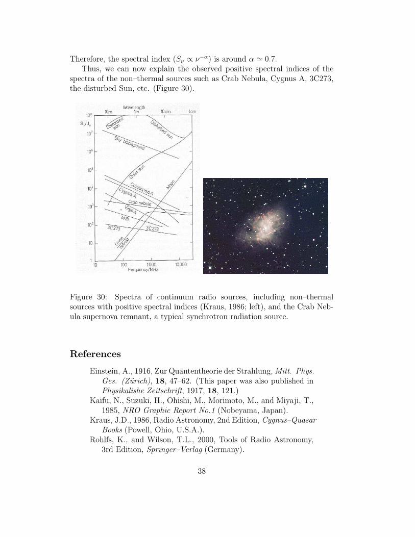
Therefore, the spectral index (Sν ∝ ν−α) is around α ' 0.7.Thus, we can now explain the observed positive spectral indices of the

spectra of the non–thermal sources such as Crab Nebula, Cygnus A, 3C273,the disturbed Sun, etc. (Figure 30).

Figure 30: Spectra of continuum radio sources, including non–thermalsources with positive spectral indices (Kraus, 1986; left), and the Crab Neb-ula supernova remnant, a typical synchrotron radiation source.

References

Einstein, A., 1916, Zur Quantentheorie der Strahlung, Mitt. Phys.Ges. (Zurich), 18, 47–62. (This paper was also published inPhysikalishe Zeitschrift, 1917, 18, 121.)

Kaifu, N., Suzuki, H., Ohishi, M., Morimoto, M., and Miyaji, T.,1985, NRO Graphic Report No.1 (Nobeyama, Japan).

Kraus, J.D., 1986, Radio Astronomy, 2nd Edition, Cygnus–QuasarBooks (Powell, Ohio, U.S.A.).

Rohlfs, K., and Wilson, T.L., 2000, Tools of Radio Astronomy,3rd Edition, Springer–Verlag (Germany).

38

Westerhout, G., 1958, A Survey of the Continuous Radiation fromthe Galactic System at a Frequency of 1390 Mc/s, Bull. As-tron. Inst. Netherlands, 14, 215.

39