Using On-line Simulation in UAV Path Planning - DiVA portal12687/FULLTEXT01.pdf · Using On-line...
110
Using On-line Simulation in UAV Path Planning FARZAD KAMRANI Licentiate Thesis in Electronics and Computer Systems Stockholm, Sweden 2007
Transcript of Using On-line Simulation in UAV Path Planning - DiVA portal12687/FULLTEXT01.pdf · Using On-line...

Using On-line Simulation in UAV Path Planning
FARZAD KAMRANI
Licentiate Thesis in Electronics and Computer SystemsStockholm, Sweden 2007

TRITA-ICT/ECS AVH 07:06ISSN 1653-6363ISRN KTH/ICT/ECS AVH-07/06–SE
Akademisk avhandling som med tillstånd av Kungl Tekniska högskolan framläggestill offentlig granskning för avläggande av filosofi licentiatexamen måndagen den 3dec 2007 klockan 15.00 i Sal D, Forum, Isafjordsgatan 39, Kista.
© Farzad Kamrani, November 2007
Tryck: Universitetsservice US AB

iii
Abstract
In this thesis, we investigate the problem of Unmanned Aerial Vehicle (UAV) pathplanning in search or surveillance mission, when some a priori information about thetargets and the environment is available. A search operation that utilizes the availablea priori information about the initial location of the targets, terrain data, and informationfrom reasonable assumptions about the targets movement can in average perform betterthan a uniform search that does not incorporate this information. This thesis providesa simulation-based framework to address this type of problem. Search operations aregenerally dynamic and should be modified during the mission due to new reports fromother sources, new sensor observations, and/or changes in the environment, therefore aSymbiotic Simulation method that employs the latest data is suggested. All availableinformation is continuously fused using Particle Filtering to yield an updated picture ofthe probability density of the target. This estimation is used periodically to run a setof what-if simulations to determine which UAV path is most promising. From a set ofdifferent UAV paths the one that decreases the uncertainty about the location of the tar-get is preferable. Hence, the expectation of information entropy is used as a measure forcomparing different courses of action of the UAV. The suggested framework is appliedto a test case scenario involving a single UAV searching for a single target moving on aroad network. The performance of the Symbiotic Simulation search method is comparedwith an off-line simulation and an exhaustive search method using a simulation tool de-veloped for this purpose. The off-line simulation differs from the Symbiotic Simulationsearch method in that in the former case the what-if simulations are conducted before thestart of the mission. In the exhaustive search method the UAV searches the entire roadnetwork. The Symbiotic Simulation shows a higher performance and detects the targetin the considerably shorter time than the other two methods. Furthermore, the detectiontime of the Symbiotic Simulation is compared with the detection time when the UAV hasthe exact information about the initial location of the target, its velocity and its path.This value provides a lower bound for the optimal solution and gives another indicationabout the performance of the Symbiotic Simulation. This comparison also suggests thatthe Symbiotic Simulation in many cases achieves a “near” optimal performance.

iv
Sammanfattning
I detta arbete undersöks problemet av hur en obemannad luftfarkosts (UAV) färdväg iett sökuppdrag eller bevakningsuppdrag ska bestämmas givet att förhandsinformation ommålet och miljön är tillgänglig. En sökoperation som utnyttjar den tillgängliga förhands-informationen om målets utgångsläge, terrängdata, och rimliga antaganden om måletsrörelse, kan i medel prestera bättre än en likformig sökning som inte tar hänsyn till dennainformation. Detta arbete tillhandahåller ett simuleringsbaserat ramverk för att besvaradenna fråga. Bevakningsoperationer är i allmänhet dynamiska och bör modifieras underuppdragets gång på grund av nya rapporter från andra källor, nya sensorobservationer,och/eller ändringar i miljön, därför föreslås en symbiotisk simuleringsmetod som använ-der sig av den senaste informationen. All tillgänglig information bearbetas kontinuerligtmed hjälp av en particle filter metod för att producera en ständigt uppdaterad bild avmålets sannolikhetsfunktion. Denna uppskattning används periodvis för att köra en seriewhat-if simuleringar med vars hjälp det går att avgöra vilka av UAV färdvägar är de mestlovande. Från en mängd olika UAV färdvägar, är den som minskar osäkerheten om måletsläge att föredra. Därför, har väntevärdet hos informationsentropin använts för att jämföraolika UAV handlingsplaner. Det föreslagna ramverket har tillämpats på ett testscenariosom gäller en UAV som söker ett mål som rör sig på ett vägnätverk. Prestandan hos densymbiotiska simuleringssökmetoden har jämförts med en ej direktansluten simulerings-metod samt en uttömmande sökmetod genom att använda ett simuleringsverktyg somhar utvecklats för detta ändamål. Den ej direktanslutna simuleringssökmetoden skiljer sigfrån den symbiotiska simuleringssökmetoden genom att what-if simuleringarna genomförsinnan uppdraget startas. I den uttömmande sökmetoden söker UAVn igenom hela vägnät-verket. Den symbiotiska simuleringssökmetoden visar en högre prestanda och har visat sigupptäcka målet på avsevärt kortare tid. Dessutom har upptäcktstiden för den symbiotiskasimuleringssökmetoden jämförts med upptäcktstiden när UAVn har den exakta informa-tionen om målets initieringsläge, dess hastighet och färdväg. Detta värde tillhandahållerett undre gräns för den optimala lösningen och ger en annan indikation om prestandan avden symbiotiska simuleringssökmetoden. Denna jämförelse har också visat att den symbi-otiska simuleringssökmetoden har många gånger en “nära” optimal prestanda.
v
Acknowledgments
This research was financed by the Swedish Defence Research Agency (FOI) andcarried out at the school of Information and Communication Technology (ICT) atthe Royal Institute of Technology (KTH).
First and foremost, I am especially grateful to my supervisor and mentor Prof.Rassul Ayani at Department of Electronic and Computer Systems (ECS) at ICTfor his constantly encouraging guidance and support throughout this research.
Many thanks to Farshad Moradi at FOI who has been the project manager ofthis research. Without his patience and constructive critiques this work would nothave been possible. Moreover, I wish to express my deepest thankfulness to mysupplementary supervisors Pontus Svenson at FOI and Robert Rönngren at ICT,who always found time to guide my research and help me.
I wish to thank Marianela Garcia Lozano at FOI for enjoyable research coop-eration resulted in a joint publication. Also many thanks to all my colleagues atKTH and FOI for their instructive discussions and challenging conversations.
I would also like to thank my opponent Prof. Stephen John Turner from NTUfor his constructive critiques on a draft of this thesis.
Finally, I wish to thank all my dear family members and friends who have beenpatient with me, and have given me emotional support throughout the work.

Contents
Contents vii
I An Overview of UAV Path Planning 1
1 Introduction 31.1 Background and Motivation . . . . . . . . . . . . . . . . . . . . . . . 31.2 Problem Formulation . . . . . . . . . . . . . . . . . . . . . . . . . . . 41.3 Thesis Outline . . . . . . . . . . . . . . . . . . . . . . . . . . . . . . 5
2 UAV 72.1 UAV: A Short History . . . . . . . . . . . . . . . . . . . . . . . . . . 72.2 UAV Applications and Categories . . . . . . . . . . . . . . . . . . . . 142.3 UAV Autonomy . . . . . . . . . . . . . . . . . . . . . . . . . . . . . . 162.4 UAV Path Planning Approaches . . . . . . . . . . . . . . . . . . . . 18
3 Employed Methodologies 253.1 Symbiotic Simulation (S2) . . . . . . . . . . . . . . . . . . . . . . . . 253.2 Particle Filtering . . . . . . . . . . . . . . . . . . . . . . . . . . . . . 27
4 Contribution of the thesis 334.1 A Brief Summary of Published Papers . . . . . . . . . . . . . . . . . 334.2 Conclusion and Future Work . . . . . . . . . . . . . . . . . . . . . . 35
Bibliography 37
II Published Papers 43
5 Paper 1 455.1 Introduction . . . . . . . . . . . . . . . . . . . . . . . . . . . . . . . . 475.2 Methodology . . . . . . . . . . . . . . . . . . . . . . . . . . . . . . . 495.3 S2-Simulator . . . . . . . . . . . . . . . . . . . . . . . . . . . . . . . 52
vii

viii CONTENTS
5.4 Future Work . . . . . . . . . . . . . . . . . . . . . . . . . . . . . . . 575.5 Conclusion . . . . . . . . . . . . . . . . . . . . . . . . . . . . . . . . 585.6 Acknowledgment . . . . . . . . . . . . . . . . . . . . . . . . . . . . . 58
Bibliography 59
6 Paper 2 616.1 Introduction . . . . . . . . . . . . . . . . . . . . . . . . . . . . . . . . 636.2 Problem Formulation . . . . . . . . . . . . . . . . . . . . . . . . . . . 646.3 Exhaustive Search . . . . . . . . . . . . . . . . . . . . . . . . . . . . 656.4 Our Aproach . . . . . . . . . . . . . . . . . . . . . . . . . . . . . . . 686.5 Test and Evaluation . . . . . . . . . . . . . . . . . . . . . . . . . . . 746.6 Future Work . . . . . . . . . . . . . . . . . . . . . . . . . . . . . . . 786.7 Conclusion . . . . . . . . . . . . . . . . . . . . . . . . . . . . . . . . 78
Bibliography 81
7 Paper 3 837.1 Introduction . . . . . . . . . . . . . . . . . . . . . . . . . . . . . . . . 857.2 Path Planning Approaches . . . . . . . . . . . . . . . . . . . . . . . . 867.3 Symbiotic Simulation . . . . . . . . . . . . . . . . . . . . . . . . . . . 877.4 Test and Evaluation . . . . . . . . . . . . . . . . . . . . . . . . . . . 957.5 Conclusions and Future Work . . . . . . . . . . . . . . . . . . . . . . 98
Bibliography 101

Part I
An Overview of UAV PathPlanning
1

Chapter 1
Introduction
1.1 Background and Motivation
An Unmanned Aerial Vehicle (UAV), is a powered pilotless aircraft, which is con-trolled remotely or autonomously. UAVs are currently employed in many militaryroles and a number of civilian applications. A more detailed definition of UAVs isprovided in Chapter 2. The two basic approaches to implementing unmanned flight,remote control and autonomy, rely predominantly on communication (data link)and microprocessor technology. While both technologies are used to different levelsin all current UAVs, it is these two technologies that compensate for the absence ofan on-board pilot and thus enable unmanned flight [1]. Since the introduction ofthese technologies, the advances in them have grown exponentially. Even if thereis no evidence that these trends will continue at the same rates, the expectation isthat the computational power and communication technology will continue to growrapidly. This implies that methodologies that were not feasible for UAVs due toconstraints on the computational power and/or communication bandwidth alreadyare, or will be applicable in the near future. While advances in communicationtechnology and ongoing work in human-machine interaction, ultimately can makethe physical presence of a pilot in the aircraft completely unnecessary, advances inmicroprocessors, control technologies and different fields of computer science candramatically improve the capabilities of the UAV to address more complicated taskswith less oversight of human operators, a feature generally called autonomy. Au-tonomy technology will stretch the boundary of what is possible to accomplish infuture missions, by overcoming limitations due to communications delays, missioncomplexity and cost. Increasing computational power on-board does not automat-ically lead to autonomy, however, it is one major prerequisite of an autonomoussystem. This computational power is now available at low costs.
To overcome the limitations of a single platform and address more complicatedand challenging tasks, the idea of employing teams of cooperating UAVs is fre-quently discussed. A team of cooperating UAVs may conduct different types of
3
4 CHAPTER 1. INTRODUCTION
operations e.g. in areas such as urban warfare, wide area search/attack, assess-ment of geographically dispersed targets and time-critical rescue operations. Thisconcept is developed further to a swarm of (Micro) UAVs collaborating for a jointmission, by sharing information and distributed control. However, these steps re-quire significant investments in distributed control technology [1].
Despite magnificent achievements, the autonomy technology has not yet beendeveloped to utilize the full power of increasing micro-processor performance. Thefield of autonomous systems is interdisciplinary and uses techniques and insightsfrom multiple fields including artificial intelligence, operational research, controltheory, optimization, robotics, computer vision, data fusion and information theory.Autonomy is context-dependent. The mission to be accomplished autonomouslydefines the tasks and the required methods to address them. The preliminaryaim of packing more “intelligence” into the UAV is to support the operator of theUAV to cope with more complex tasks, but it may well in the future eliminatethe necessity of a human operator or reduce the role of the operator to high-levelapproval of decisions made by the machine.
1.2 Problem Formulation
In civil aviation flights and many military flight missions the aircraft’s freedom ofaction and movement is restricted and the path is predefined. Given the path thecontrol task of the aircraft is to generate the trajectory, i.e. to determine requiredcontrol maneuvers to steer the aircraft from one point to another. However, insome flight missions the path is not predefined but should dynamically be deter-mined during the mission, e.g in military surveillance, search & rescue missions,fire detection and disaster operations. In this type of scenarios the goal of the UAVis to find the precise locations of searched objects in an area given some a prioribut often uncertain information about the initial state of the objects. Since duringthe search operation this information may be modified due to new reports fromother sources or the UAVs observation, the path of the UAV can not be determinedbefore starting the mission. One way to address the problem is to search the areaof interest uniformly. To increase the utilization of the UAV resources, the operatorcan conduct the search operation in a manner that areas with higher probability offinding the objects are prioritized and/or searched more thoroughly. When somenew information is available this process may be repeated and if necessary a newpath for the UAV is planned. There are two drawbacks with this approach. Firstly,it is not always a trivial task to determine areas with higher probability of findingobjects, since both the targets and the UAV move. Analysis of this information maybe beyond the capacity of a human brain. Secondly, due to the time-critical natureof these missions, it is not feasible to assign this task to an operator. Valuable timemay be lost before information is processed by the human operator and it may beimpossible to fulfill the time requirements. These arguments are particularly validif the scenario is dynamic and new information arrives during the mission.

1.3. THESIS OUTLINE 5
A more efficient approach is to automate the path planning process and integratethe reasoning about the locations of the targets into the autonomous control systemof the UAV. In order to make this possible all available information has to beconveyed to the UAV and the autonomous control system of the UAV has to becapable to plan its route. Moreover, the UAV should dynamically modify its routewhen more information is available.
Additional criteria such as decreasing the operational costs and minimizing therisk of being detected may be incorporated into the primary objective of maximizingthe probability of locating targets.
In this thesis a general framework for solving this problem is introduced andto investigate the feasibility of the method a test case scenario has been studied.In this test case scenario a UAV searches for a single target moving with a givenprobability on a known road network.
1.3 Thesis Outline
Chapter 2 gives a brief history of UAV development and highlights some eventsin the history of operational use of UAVs. A possible classification of UAVs isintroduced and their potential application areas are presented. Some aspects ofautonomous systems important to UAV are discussed and a survey of path planningresearch is given and our approach to the problem is introduced.
Chapter 3 presents the methodologies employed in this thesis. The concept ofSymbiotic Simulation is presented and an introduction to Sequential Monte Carlomethods also called Particle Filtering is given.
Chapter 4 Gives a short description of three papers published in conferenceproceedings, which contains the main contribution of this thesis.
Part II The main contribution of this thesis have been published in conferenceproceedings as described below:
1. Farzad Kamrani, Marianela Garcia Lozano, and Rassul Ayani. Path Planningfor UAVs Using Symbiotic Simulation. In Proceedings of the 20th annual Eu-ropean Simulation and Modelling Conference, ESM’2006, Toulouse, France,October 2006.
2. Farzad Kamrani and Rassul Ayani. Simulation-aided Path Planning of UAV.To appear in Proceedings of the Winter Simulation Conference, WSC’07,Washington, D.C., December 2007.
3. Farzad Kamrani and Rassul Ayani. Using On-line Simulation for AdaptivePath Planning of UAVs. In Proceedings of the 11-th IEEE InternationalSymposium on Distributed Simulation and Real Time Applications, Chania,Crete Island, Greece, October 2007.

Chapter 2
UAV
An Unmanned (Uninhabited) Aerial Vehicle (UAV) is defined as: “A powered, aerialvehicle that does not carry a human operator, uses aerodynamic forces to providevehicle lift, can fly autonomously or be piloted remotely, can be expendable orrecoverable, and can carry a lethal or non-lethal payload. Ballistic or semi ballisticvehicles, cruise missiles, and artillery projectiles are not considered unmanned aerialvehicles” [2]. This definition excludes cruise missile weapons even though theyare unmanned, with the motivation that (1) UAVs are equipped and intended forrecovery at the end of their flight, and cruise missiles are not, and (2) munitionscarried by UAV are not tailored and integrated into their airframe whereas thecruise missile’s warhead is [1, 3]. However, one more strong reason is that dueto the international agreements that regulate and limit nonnuclear missiles, it isdisadvantageous to categorize missiles as UAVs. In recent literature the terminologyUnmanned Aircraft System (UAS) is used rather than UAV to emphasize that theaircraft is only one component of the system. Using this terminology the termUnmanned Aircraft (UA) is adopted when referring to the flying component ofthe system. Through this text we use the term UAV to refer to both the flyingcomponent as defined above and the whole system. Sometimes the term drone,which was common before the term UAV was established is employed, especiallywhen referring to older model of UAVs.
2.1 UAV: A Short History
From the early days of developing the so called flying bombs, i.e. pilotless aircraftscarrying bombs in 1916, up to now, UAVs have served various purposes, mainly inmilitary applications. The design and development of the UAVs have been stronglycharacterized by the requirements of military conflicts in different eras. To providean insight into the variation of these requirements and UAV categories a relativelybrief history of UAV is given in this Section. This survey is far from complete,
7
8 CHAPTER 2. UAV
however, it highlights events and milestones that have shaped the development ofthe UAVs. A detailed reference to the history of the UAV is provided by [4–6].
Pre-aviation Period
In 1849, the Austrians launched some 200 pilotless balloons against the city ofVenice. The balloons each carried a 15 kg explosive payload controlled by time fuses.Some bombs exploded as planned but the wind changed direction and blew severalballoons back over the Austrian lines. This is, the first recorded use of unmannedflight devices in a military context [7]. During the American Civil War, an inventornamed Charles Perley registered a patent for an unmanned aerial bomber whichwas a hot-air balloon carrying a basket laden with explosive attached to a timingmechanism. The timer would drop out the explosive and ignite a fuse [8]. BothUnion and Confederate forces are said to have launched Perley’s balloons duringthe war, with limited success.
Kites had been used to investigate the atmosphere in the mid-eighteenth century.The first kite-borne atmospheric measurements were reported in 1749 by ProfessorAlexander Wilson and his student Thomas Melville, both of the University of Ed-inburgh, Scotland. Wilson’s kite experiments were followed in 1752 by the famousatmospheric electricity experiment of Benjamin Franklin near Philadelphia [9]. In1882, English meteorologist E. D. Archibald took the first successful photographsfrom kites. R. Thiele, a Russian government councilor, connected seven unmannedkites and mounted cameras on them in 1889. The obtained panorama pictureswere employed for cartographic recording and interpretation of remote areas [10].American meteorologist W. A. Eddy made what he claimed was the first kite photoever taken in the Western Hemisphere on May 30, 1895. During the Spanish Amer-ican War, his system was used in Puerto Rico, where it was a valuable addition toballoon photography [10].
Early Target Drones
Marconi’s first successful wireless transmission in 1896 and the invention of theairplane less than a decade later opened the technological fields of electronics andaviation. One of the many areas of utilization in which these two fields have mergedis pilotless aircraft. The first pilotless aircraft built during and after the first worldwar was intended to be used as “flying bombs”. Without the advanced technologiesavailable in more recent years, the only way to control a pilotless aircraft is tocontrol it remotely. Nikola Tesla who obtained a patent for remote control in 1898is credited for the concept of remote control. He demonstrated the possibility toremote control a 2 meter boat in an artificial lake by radio waves [5]. In 1916-1917, Peter Cooper Hewitt and Elmer A. Sperry invented the automatic gyroscopicstabilizer, which helps to keep an aircraft flying straight. Without this technologicalbreakthrough, it was not possible to efficiently control an aircraft by radio control.Hewitt and Sperry used this gyroscopic stabilizer to convert a U.S. Navy Curtiss
2.1. UAV: A SHORT HISTORY 9
N-9 trainer aircraft into the first radio-controlled flying bomb [5]. Developmentof the flying bomb involved solving several serious interrelated problems. It wasnecessary to obtain a feasible airframe, find a way to launch a pilotless vehicle andmake sure that the control mechanism would operate after a pilotless launch. TheHewitt-Sperry Aerial Torpedo flew 80 to 150 km carrying a 150 kg bomb in severaltest flights [5, 7].
Army representatives witnessed one of these flights and started a similar aerialtorpedo, or flying bomb, project led by Lieut. Col. Bion J. Arnold for the AirService and Charles Kettering for industry. Kettering Aerial Torpedo, nicknamedthe "Bug", was made of wood and canvas and launched from a four-wheeled dollythat ran down a portable track. The Bug’s system of internal pre-set pneumatic andelectrical controls stabilized and guided it toward a target. After a predeterminedlength of time, a control closed an electrical circuit, which shut off the engine.Then, the wings were released, causing the Bug to fall to earth – where its 100 kgof explosive detonated on impact. The Dayton-Wright Airplane Co. built fewerthan 50 Bugs before the end of the war, and the Bug never saw combat. After thewar, the U.S. Army Air Service conducted additional tests, but further developmentwas halted in the 1920s, due to the lack of financial resources [11].
The DH.82B Queen Bee built in UK, is the first returnable and reusable pilotlessaircraft which fulfills the definition of a UAV. It was designed for use as an aerialtarget for training anti-aircraft gunners in the Royal Navy in 1935 and they werein use until 1947. DH.82B Queen Bee was radio controlled and could fly as high as5000 m and travel a maximum distance of 500 km at over 175 km/h [4].
Radioplanes
In 1939, Englishman and Hollywood actor Reginald Denny formed the RadioplaneCompany in Los Angeles. This company designed and produced low-cost radiocontrolled aircraft for hobbyists, but Reginald Denny was convinced that theseradioplanes could be used as a training means for anti-aircraft units. In 1940,the company won a contract with the US Army and produced more than fifteenthousand OQ-2 Radioplanes during the second world war. OQ-2 is the first mass-produced UAV [4].
Modern Target and Decoy UAVs
The main area of use for UAVs until the end of the second world war was as targetdrones. This trend continued after the war. The Ryan Firebee, was a series of targetdrones developed by the Ryan Aeronautical Company. It was the first jet-propelledUAV, and one of the most widely employed drones ever built [12].
Another area where pilotless aircraft can be employed is as decoys. The firstexperiments with using a UAV as decoy was in the 1950s, when a GAM-67 “Cross-bow” was tested in this role. In the 1950s, the USA was becoming concerned aboutthe ability of its strategic bombers to penetrate Soviet air-defense systems and
10 CHAPTER 2. UAV
reach their targets in the face of rapidly improving radar, jet fighters and surface-to-air missile systems. A major US effort to develop radar-visible decoy missileswas begun. The idea was that if each bomber launched several such missiles, theSoviet defense would have to deal with many more targets, giving the real bombersa much higher chance of getting through. The developed system, which was namedDAM-20 “Quail”, was the first operational UAV serving as a decoy. Each B-52could carry up to eight Quail drones [13].
Reconnaissance UAVs
The use of UAVs in reconnaissance missions appears later. A reconnaissance aircraftshould be stealth, i.e. its radar signature should be as small as possible. A targetdrone is the opposite, it should have a radar signature near that of the aircraft itsimulates. However, reducing the radar signature of a UAV is easier than reducingthe radar signature of a manned aircraft, since constraints on the size and shaperelated to carrying a pilot is removed. In the late 1950s, Ryan Aeronautical wasinvestigating the possibility of using the company’s Firebee target drone for long-range reconnaissance missions primarily for flying over the Soviet Union. Thesereconnaissance drones were planned to be launched from the Barents sea and re-covered in Turkey and could substitute the Lockheed U-2 spy planes. In May 1960,an American U-2 spy plane over the Soviet Union and later the same year a BoeingRB-47 which probed Soviet airspace were shot down. These incidents increasedthe interest of the US Air Force for reconnaissance UAVs. Although the modifiedFirebee target drone, named Ryan Model 147A “Fire Fly” was a success it was notused operationally [4]. The successor of the Fire Fly, which was given the nameRyan Model 147B “Lightning Bug” was the first operational reconnaissance UAV.It was launched from a DC-130 airplane, completed its reconnaissance mission overChina and returned to Taiwan. Lightning Bug and its successors, which all weresmaller versions of Firebee, were used continuously in the Vietnam War during 1965-1975 [14]. These UAVs were mostly air-launched, and after their mission they weredirected to a safe recovery area, where they deployed their parachutes and wererecovered in mid-air by a helicopter before landing. They were very reliable. Morethan 1000 UAVs flew about 34000 operational surveillance missions over SoutheastAsia until the end of the war. During these years, other projects to build UAVswith higher performance (higher altitude, longer endurance, higher speed) or othercapabilities, were initiated and supported by US military. As an example of suchambitious programs, the Lockheed D-21 “Tagboard” can be mentioned. Tagboardwas an advanced reconnaissance drone produced in secret having a velocity over 3Mach. The project did not lead to any success. Although these projects may havecontributed to the field, none of them resulted in production of operational UAVson a significant scale.

2.1. UAV: A SHORT HISTORY 11
Battlefield UAVs
The next step in developing UAVs was taken by Israelis. After the 1973 Arab-Israeli War, the Israeli military were concerned about the substantial losses ofaircrafts caused by Soviet Union built Surface-to-Air Missiles (SAM) during thewar and were searching for new technologies to prevent the problem in future wars.Reconnaissance UAVs so far were suited for “strategical reconnaissance”, while theyneeded UAVs for “tactical reconnaissance” or “combat surveillance”. The Israelimilitary and air industry built a series of so called battlefield UAVs in late 1970s toaddress this problem. Mastiff, Scout and Searcher were all relatively small UAVswith an empty weight less than 100 kg. They all had an autopilot system withradio control backup and could be launched and recovered using runways (otherlaunch and recovery schemes were also possible). They featured pusher-propellersand had a relatively long endurance between 7 and 12 hours. Mastiff and ScoutUAVs were operating in the invasion of southern Lebanon starting in 1982 and haveproven successful [4].
Endurance UAVs
In the late 1950s, using UAV helicopters powered by beaming microwave for atmo-spheric observations as a less costly alternative to satellites, was suggested. A seriesof experiments were conducted in 1964 including one flight with ten continuoushours at an altitude of 15 meters [15]. Despite good publicity of the demonstra-tion, the concept did not develop further at that time. However, experiments with“unconventional” power systems to design High-Altitude Long-Endurance (HALE)UAVs continued later. McSpadden et al. presents several demonstrations of mi-crowave powered UAVs performed during 1986 to 1995, including the CanadianStationary High Altitude Relay Platform (SHARP) [16].
Another “unconventional” power source for aircrafts is solar power. In 1981,after a manned solar-powered aircraft accomplished a 262 km flight from Paris toRAF Manston in the UK, the concept of solar-powered HALE UAV came intoprominence. In 1983, a secret project, named High Altitude Solar (HALSOL),conducted by AeroVironment and funded by an unspecified US government agencywas started to examine the idea [4]. The result of the project was a flying wingwith a span of 30 meters propelled by eight electric motors. However, the solarcell technology at the time was not mature enough to be able to supply the neededelectrical power. The project was terminated but the aircraft was stored. Ten yearslater, the aircraft was retrieved and equipped with solar cells under the ResponsiveAircraft Program for Theater Operations (RAPTOR) program. The upper surfaceof the UAV’s wings was covered with solar panels that supplied enough electricity todrive its small electric motors and it was renamed RAPTOR/Pathfinder. The roleof this solar-powered endurance UAV was to provide long-range sensors and assistanother UAV named RAPTOR/Talon to target tactical ballistic missiles. Theproject was abandoned due to financial problems, but the RAPTOR/Pathfinder
12 CHAPTER 2. UAV
was handed over to the National Aeronautics and Space Administration (NASA)and operated under the name Pathfinder in the Environmental Research Aircraftand Sensor Technology (ERAST) project. In 1997, the Pathfinder established thealtitude record for a propeller-driven aircraft reaching an altitude of over 21,650meters. A prototype of the successor of Pathfinder, the solar-powered UAV Helioswith a wingspan of 75.3 meters and fourteen electric motors established an absolutealtitude record of 29,420 meters, in 2001. The aircraft disappeared in a crash in2003 [4].
Attempts to design endurance UAVs were not limited to microwave-beamed orsolar-powered aircrafts. On the contrary the main stream of research was focusedon UAVs propelled by conventional fuel. The first long endurance UAV was builtin the early 1970s during the Vietnam War and was supposed to operate as a radiorelay to collect data from air-dropped acoustic sensors with limited range. TheUAV was designated XQM-93 and could stay aloft for 30 hours carrying a payloadof 320 kg. XQM-93 was never used in operations.
In the mid-1980s Boeing, in cooperation with the Defense Advanced ResearchProjects Agency (DARPA), developed a super-secret HALE UAV named the Con-dor, which pioneered a number of innovations for future endurance UAVs [4]. TheCondor, with 61 meters wingspan, is one of the largest wing-span aircrafts everbuilt. Its empty weight was 3630 kg, which is very low for its size. About 60% ofthe Condor’s loaded weight (9070 kg) was fuel. The Condor was built of state-of-the-art carbon fiber composite materials, giving it stealth qualities. With a verylow radar and heat signature footprint, the Condor was nearly electronically invis-ible. Its service ceiling was 20000 meters and it could stay aloft more than 2.5 dayscarrying a 815 kg payload. The Condor was equipped with two identical controlcomputers running the same program providing a redundant and reliable flight con-trol. The control system was pre-programmed and the Condor could operate fullyautonomously including an automated takeoff and landing without any interventionof the operator. However, it was possible to to modify a mission during the flight.The Condor featured some degree of automated failure management allowing it torecover from certain in-flight emergencies. The Condor was never used in operationand is now hanging from the ceiling of the Hiller Aviation Museum [5].
Another secret program which ran parallel with the Condor, was Amber [4]. In1984, DARPA issued a 40 million dollar contract to Leading Systems Incorporated(LSI), to develop an endurance UAV which was meant to be used for photographicreconnaissance, electronic intelligence, or as a cruise missile. Amber was relativelysmall, weighed 335 kg and could remain 38 hours in the air. Amber successfullycompleted its first flight in 1989 but due to reduced funding the project was aban-doned. General Atomics purchased LSI later and completed a simplified variant ofthe Amber, namedGnat 750, which led to a contract with the Turkish governmentin 1993. The US government also showed interest for Gnat 750. They were to beoperated by the Central Intelligence Agency (CIA) in former Yugoslavia for recon-naissance. Gnat 750 is a relatively small UAV, with a maximum loaded weight of517 kg and 48 hours endurance. The well-known UAV Predator which is currently

2.1. UAV: A SHORT HISTORY 13
in service in the wars in Afghanistan and Iraq, is an enlarged and more capablederivative of the Gnat 750.
Current Endurance UAVs
Endurance UAVs play an increasingly strategic role in airborne surveillance andcollection of intelligence, and even in strike missions. The first endurance UAV, thePredator recently (June 2007) achieved 300000 flight hours [17]. RQ-1 Predatorwhich is an improved Gnat 750 is a relatively small aircraft, with a max gross takeoffweight of 1043 kg and a maximum endurance of 40 hours. In 1995 Predator was forthe first time used in operations in conflicts in former Yugoslavia for reconnaissanceand surveillance. The experience in former Yugoslavia showed the difficulties ofusing the information acquired by the UAVs to strike mobile ground targets. Thetarget often disappeared before an attack aircraft reached the area. The USAFdesire to possess strike UAVs led to arming Predator with Hellfire Air-to-GroundMissile System (AGMS) and the introduction of Unmanned Combat Aerial Vehicle(UCAV) (discussed later).
Another operating endurance UAV used for strategic reconnaissance is theNorthrop Grumman’s Global Hawk. It is a relatively large HALE UAV, with agross takeoff weight of 12110 kg, a payload of 970 kg, and a maximum enduranceof 35 hours. Global Hawk is equipped with long-range sensors and can survey largeareas from distance without being exposed to hostile air defense. Northrop Grum-man is currently working on an improved and larger version of Global Hawk witha payload of up to 1360 kg.
Other endurance UAVs around the world are the E-Hunter, Heron, Hermes 450and Hermes 1500 all developed by Israelis. Heron has an endurance of 50 hours.BAE Systems has recently developed High Endurance Rapid Technology Insertion(HERTI) with an endurance of up to 30 hours for surveillance and reconnaissancein military and civil operations. The Russian Sukhoi Company (JSC) is currentlydesigning three endurance UAVs, designated Zond 1, Zond 2 and Zond 3 [4].
Unmanned Combat Aerial Vehicle (UCAV)
As discussed earlier, unpiloted aircrafts were from the very beginning intended tobe used as flying bombs. In the early 1960s the modern UAVs, i.e. unmannedaircrafts that autonomously or by the assistance of a remote control could fly toan area and return were a reality. The early “flying-bombs” had evolved to cruisemissiles and the UAVs were operated mainly in reconnaissance missions or as tar-gets and decoys. But if UAVs could carry sensors they could carry munitions aswell. The idea of Unmanned Combat Aerial Vehicle (UCAV), i.e. a UAV thatis armed and is used in combat missions, was not very far-fetched to the military.Ryan Aeronautical was the first company which experimented with the idea in 1964arming a Firebee with two 115 kg bombs. The experiment, called Project CeeBeedid not lead to any immediate progress. However, in 1971, when guided weapons
14 CHAPTER 2. UAV
were available the concept became popular again. Attack UAVs were meant to beused for Suppression of Enemy Air Defenses (SEAD) which is hazardous by natureand suited for UAVs. Despite successful experiments the idea was abandoned in1979. The technology simply was not mature enough for this concept, communi-cation links were not reliable and the Command and Control (C2) problems wereapparent. Introduction of the Global Positioning System (GPS), establishment ofmore reliable communication links and more mature autonomous technologies inthe next two decades were required before the concept of UCAV could seriouslybe discussed again. As mentioned, the first UAV which was used in active combatwas Predator, a reconnaissance UAV armed with Hellfire missiles. A series of testswas first performed in February 2001, showing that the idea was feasible and laterthat year the Predator carrying Hellfire missiles were operating in the Afghanistanwar [6].
UAVs under Development
The USAF Boeing X-45, the US NAVY Northrop Grumman X-47 UCAV and theEuropean Neuron are under development. In order to merge the efforts of USAFand US NAVY in developing UCAVs the Joint Unmanned Combat Air System (J-UCAS) program under DARPA direction was started. J-UCAS has recently beendissolved.
Common for these projects and other ongoing projects is the ambition to in-crease the level of autonomy in the UAVs. Some of the tasks related to UAV auton-omy are partially or completely solved and others are subject to intensive research.As an example, recently the DARPA completed its Autonomous Airborne Refuel-ing Demonstration program, showing that unmanned aircraft can autonomouslyperform in-flight refueling under operational conditions [18].
2.2 UAV Applications and Categories
Currently, some 32 nations are developing or manufacturing more than 250 modelsof UAVs and 41 countries operate some 80 types of UAVs [1]. By all accountsutilization of UAVs in military and public/civilian application is expanding both inthe short term and long term. There are at least three categories of tasks whereUAVs are the only solution or provide a preferred solution over manned aircraft.
First, in presence of physical constraints on the size of the aircraft such that,the smallest manned aircraft is not feasible, e.g. searching for survivors in burningbuildings or damaged structures, which may be performed only by so called microUAVs. In such cases the UAV cannot be substituted by a manned aircraft.
Second, whenever a task is preferred to be performed by UAVs, i.e. when itbelongs to what military call “dull, dirty or dangerous”. Example of “dull” tasksare long time surveillance missions. Tasks are “dirty” if the pilot and the aircraftare exposed to hazardous materials, e.g. flying in nuclear clouds. Missions are
2.2. UAV APPLICATIONS AND CATEGORIES 15
“dangerous” if they involve extreme exposure to hostile actions, e.g. reconnaissancemissions and SEAD operations [3].
Third, when the UAV solution is more cost effective than the manned counter-part, e.g. if in the future the airworthiness of UAVs are certified and they can fly incivilian airspace, they will provide a more cost effective solution than the mannedalternative in cargo flights.
UAVs can be classified in two main categories, military and civilian. The use ofUAV in military applications which has been discussed so far can be summarizedas the following roles:
• Target, Decoy and Deception
• Reconnaissance and Surveillance
• Targeting and Strike
• Communication Relay
Various systems for categorization of UAVs in military operations have been sug-gested. US Military uses a “Tier” system to designate the role of various aircraftelements. Three tiers, Tier I, Tier II and Tier III are introduced, where transi-tion from Tier I to Tier III is from low altitude to high altitude and from shorterendurance to longer endurance. However, US Army, USAF and US Navy each hasits own tier systems which are not integrated among themselves. One generallyaccepted classification of the UAVs is the following:
• Short- to medium-range UAVs
• Medium Altitude Long Endurance (MALE) UAVs
• High Altitude Long Endurance (HALE) UAVs
• Unmanned Combat Aerial Vehicles (UCAVs)
• Miniature or Micro UAVs
There are a wide range of civil applications for which UAVs may prove useful.Desired future missions of civil UAVs based on user defined requirements are deter-mined and documented in a report from NASA [19]. In this report four categoriesare distinguished and in each category several mission types are discussed. Thissurvey is partly based on a series of personal interviews with subject matter expertsin private and public sector organizations, which have shown interest as potentialusers of UAVs. Although some of the mission types discussed in [19] appear to beappropriate only for the USA and are specified in accordance with that country’srequirements, this survey gives an insight into the growing applicability of UAVsworldwide. This four categories are as follows:
1. Commercial missions. This sector is not discussed further in the report, how-ever, the following are possible applications in this sector.

16 CHAPTER 2. UAV
• Communications and broadcast services.
• Air traffic control support.
• Power transmission line monitoring.
• Precision agriculture and fisheries.
2. Earth science UAV missions. The number of mission types belonging to thiscategory is relatively large, e.g. missions related to measurements of geo-physical process such as earthquakes and volcanoes, monitoring changes instratospheric ozone chemistry, studying tropospheric air quality and distri-bution of the tropospheric pollutions, studying water vapor and measuringtotal water in the tropical tropopause layer, and measuring the dynamics ofthe breakup of polar glacier and polar ice sheets.
3. Homeland security. Missions such as coastal patrol and surveillance of mar-itime traffic, maritime search and rescue missions, border surveillance, andground transportation monitoring and control can be classified under thiscategory.
4. Land management missions.
• Forest fire damage assessment, forest fire mapping, forest fire communi-cations, and fire damage assessment.
• Conducting aerial surveys of wildlife species of interest, and animal track-ing.
• Digital mapping.
2.3 UAV Autonomy
Despite the diversity of UAV systems a clear tendency in the market and amongthe designers of UAV systems toward more autonomy is distinguishable. More het-erogeneous, autonomous, cooperative UAV systems that not only are independentof human intervention for flight control and mission control but also are capableto self-plan missions based on an understanding of the commander’s intent areseriously discussed in related literature [20].
In an attempt to categorize existing and future UAVs according to the degreeof autonomy the US Air Force Research Laboratory (AFRL) has introduced thenotion of Autonomous Control Level (ACL), and describes ten such levels, rangingfrom remotely piloted vehicles to fully autonomous swarms of UCAVs [21].
1. Remotely guided: conventional radioplanes that are controlled remotely byradio signals.
2. Real time health/diagnosis: self awareness, i.e. the ability to notice the healthstate of the UAV.
2.3. UAV AUTONOMY 17
3. Adapt to failures and flight conditions: data loss tolerance and capability toadapt to changes in weather conditions.
4. On-board route replan: changing the route to accomplish the same mission.
5. Group coordination: e.g. collision avoidance with other UAVs.
6. Group tactical replan: shared awareness state.
7. Group tactical goals
8. Distributed control
9. Group strategic goals
10. Fully autonomous swarms
UAVs that are in operational use today do not rank very high on the scale of Au-tonomous Control Levels (ACL), e.g. the Predator and the Global Hawk demon-strate an ACL in between level 2 and level 3. The DARPA-funded Joint UnmannedCombat Air Systems (J-UCAS) autonomy was planned to reach the level 6 of ACL.This goal was expected to be accomplished by 2015. However, this program wasrecently abandoned. While the concept of ACLs is widely accepted as a metric fordescribing autonomy in UAVs, the exact meaning of each level is not specified [22].For instance, ACL 4 is defined as the capability of on-board route replanning in theface of unknown situations. However if the final aim is to achieve fully autonomousswarms of UAVs this level of path planning is not sufficient. To reach this level ofautonomy, the UAV should be able to develop its own strategic goals to accomplisha particular mission, i.e. the UAV should understand missions on a higher level ofabstraction. Autonomy is context dependent and it should lead to an optimizedpartnership between the operator and the intelligent platform. The operator deliv-ers task level instructions to the UAV and monitors the system status. A high levelof autonomy does not necessarily eliminate humans from the decision loop, but itwill change the level of intervention.
One of the challenges in the design of such systems is to provide effective meansof interaction between humans and the UAV. The exact type of interaction betweena human and on-board autonomy varies widely across UAV platforms. For instance,the ground-based control station of the Predator UAV essentially resembles a tradi-tional cockpit, but in some other UAV systems the control stations allow choosinga preprogrammed route by waypoints with the possibility of modifying the routeunder flight. This is the highest level of autonomy found in currently operationalUAVs. Using one control station to control multiple UAVs is in the final stages oftest and will be operational in a near future. However, theoretical research on moreautonomous systems and experiments with these ideas are ongoing, some of themclaiming they have reached true autonomy in UAV flight [23].
The absence of a human pilot creates a huge void in the vehicle-system. A pilotprovides the capability to examine, interpret, and respond to changes in the vehicle
18 CHAPTER 2. UAV
and mission environment. Factors such as unforecasted weather changes, errorsin terrain databases, encountering previously unknown threats and the impact ofvehicle subsystem failures, which human pilots in manned aircraft routinely dealwith, should be addressed by the remote control or the autonomous system [24].These factors are mainly associated with levels 2 and 3 of ACL defined by AFRL, i.e.real time health and diagnosis and adapt to failures and flight conditions. Howevera full autonomous system demands an on-board overall decision-making capacity,which not only continues a mission when unanticipated events occur, but also canhandle the uncertainty which is inherent in the mission. As an example consider asearch and surveillance operation where some a priori information about a targetand terrain topology is available. The a priori information about the searchedobject is usually based on uncertain reports from other information sources. Theterrain topology constrains the movement of the target and if the map of the terrainis available, it should highly influence different decisions in the search operation.An autonomous UAV should consider all this available information to performits mission as effective as possible, i.e. the UAV should understand its missionand environment (situational awareness) and make routine decisions and missionrefinements.
The problem is two-fold. One is to convey all information to the UAV and theother is how this information is utilized. The first part is principally easier to solve,information about the terrain can be satellite pictures converted to digital maps.The “hot” areas can be marked on an interactive Command and Control (C2) dis-play, and possible information about the movements and signature of the objectcan be read from a data-base.
2.4 UAV Path Planning Approaches
Related Work
UAV path planning may refer to different things depending on the context in whichit is used. If the goal is to find a route visiting a given collection of points or areasunder some constraints such as path length or operational cost, then the problemcan be considered to be an optimization problem. In a military context avoidingthe adversary threats is added to the set of constraints and minimizing the risks ofhostile actions will be a crucial part of the planning. If perfect information aboutthe constraints and the threats that will be encountered are available, a safest pathcan always be constructed by solving an optimization problem [25]. However, theseproblems are multi-objective and multi-constraint optimization problems, whichare computationally very demanding. This category of UAV path planning canbe addressed by employing existing methods in robotics. Path planning problemshave been widely investigated in the robotics community. The problem of planninga path in robotic applications is to specify a continuous and obstacle-avoiding se-quence of points from the initial position to the goal position in an environmentwith static or dynamic obstacles. The online book Planning Algorithms [26] and
2.4. UAV PATH PLANNING APPROACHES 19
the exhaustive list of references therein provide a thorough review of path planningalgorithms in robotics as well as other related topics in the fields of robotics, arti-ficial intelligence, and control theory. Two excellent surveys on the topic of UAVpath and sensor planning are provided by [27, 28].
In the UAV path planning problem, adversaries can be considered as obstaclesand similar methods to those used for robot path planning, such as roadmap, celldecomposition, and potential field can be employed. However, if there are uncer-tainties in the information about the adversary threats, a different approach mustbe considered. A path planning method for UAVs in uncertain and adversarialenvironments by using a probability map is proposed in [25]. The probability mapof threats is built from a priori surveillance data, which is employed to generatea preliminary polygonal path. This path is refined in a second step to removesharp turns or vertexes in the path. The method presented in [25] is similar tothe approximate cell decomposition methods in robot path planning in that it usesdiscretized cells for path planning. A simple extension of the method to multipleUAVs is presented as well in [25]. This extension relies on the observation that theprobability of at least one of the vehicles reaching the target increases if they takedifferent routes to the target.
Another path planner for UAVs addressing the same category of problems is in-troduced in [29]. The problem addressed in this paper is designing an off-line pathplanner for coordinated navigation of UAVs and collision avoidance in a knownstatic environment. The proposed method is called Differential Evolution which isbased on Evolutionary Computation (EC) and is claimed to have a better conver-gence performance and efficiency.
Different EC-based algorithms have been employed to real-time path planningof a single UAV [30, 31] and on-line task allocation and path planning of multipleUAVs in recent years [30, 32]. Common to these methods is that they are inspiredby the evolution theory in biology. They are iterative stochastic processes in whicha population of solutions gradually converges to a more optimal solution while ge-netic operators such as reproduction, mutation and survival of the fittest influencethe evolution of the population. One problem often encountered with evolutionarycomputation is the premature convergence, which refers to the characteristic of theplanner to be trapped at a local optimal solution. To overcome premature conver-gence parallel evolution [33] in which several populations evolve simultaneously isapplied by [34].
Cognitive Emotion Layer (CEL) architecture is a novel control and navigationsystem for UAVs suggested by [35]. It is claimed to provide a single architecture forall aspects of vehicle control, from low-level flight controls to high-level adaptivedecision-making in highly uncertain environments. CEL is a biologically inspiredapproach, modeling emotional systems for control. An emotional state is a reactivetime-varying cognitive variable that responds to stimuli and mediates between astimulus and a response. It is modeled as part of transformational networks thatare designed to drive the system to desirable states. Although the feasibility of CELstill remains to be demonstrated empirically, this approach has an advantage in that
20 CHAPTER 2. UAV
the “intelligence” in the system is not mission dependent and may be employed indifferent scenarios.
The central concerns of path planning in papers discussed so far have beenobstacle avoidance and goal reaching for a single UAV and/or multiple UAV taskallocation and mission distribution. However, path planning is equally essential insearch, surveillance and tracking missions, which is the main focus of this thesis.
Work on modern search theory began in the US Navy’s Antisubmarine WarfareOperations Research Group (ASWORG) in 1942 [36, 37]. Bernard Osgood Koopmanis credited with publishing the first scientific work on the subject in 1946, Searchand Screening, which was classified for ten years before it was published [36]. Hedefined many of the basic search concepts and provided the probabilistic model ofthe optimal search for a stationary target. However, developing algorithms for op-timal search plan for moving targets started in the early 1970s and when computertechnology became more available. The next step in developing search planners wasto consider the dynamic nature of the search process. In actual search operationsoften complementary information from other sources or as a result of the searchingprocess arrive during the search and the search effort is required to be adjusted.Computer Assisted Search Planning (CASP), developed for US Coast Guard in the1970s by Richardson is a pioneer software system for dynamic planning of searchfor ships and people lost at sea [38, 39]. CASP employed Monte Carlo methodsto obtain the target distribution using a multi-scenario approach. The scenarioswere specified by choosing three scenario types and the required parameter valuesfor each scenario. A grid of cells was used to build a probability map from thetarget distribution, where each cell had a detection probability associated with it.A search plan was developed based on the probability map. Feedbacks from thesearch was incorporated in the probability map for future search plans, if the firstsearch effort did not succeed. The shortage of computer power and display tech-nique did not allow CASP to be a truly dynamic tool operating in real-time aboardaircraft. Advances in computer technology provided the possibility of developingmore feasible tools, Search And Localization Tactical decision aid (SALT) was aprototype air-antisubmarine search planner system for real-time use aboard air-craft [36]. Even though the Operations Research (OR) community has establishedthe foundation of the optimal search planning theory and contributed with manypioneering ideas to the field, in recent years other scientific communities are likelyto be more actively involved in the field.
The problem of searching for a lost target at sea by a single autonomous sensorplatform (UAV) is discussed in [40]. The target in this paper may be static ormobile but not evading. The paper presents a Bayesian approach to the problemand the feasibility of the method is investigated using a high fidelity UAV simulator.Bayesian analysis is a way to recursively combine the motion model of the targetand the sensor measurements to calculate the updated probability distribution ofthe target. Time is discretized in time steps of equal length and the distributionis calculated numerically. The search algorithm chooses a strategy that minimizesthe expected time to find the target or alternatively maximizes the cumulative
2.4. UAV PATH PLANNING APPROACHES 21
probability of finding the target given a restricted amount of time. The paperchooses one-step lookahead, i.e. the time horizon used for optimization is one timestep. Because of this myopic planning, the UAV fails to detect the target if it isoutside its sensor range. A decentralized Bayesian approach is suggested to solvethe same problem by coordinating multiple autonomous sensor platforms (UAVs)in [41, 42]. The coordinated solution is claimed to be more efficient, however, thesimulations in these papers suffer from the short time horizon as well, i.e. one-steplookahead.
The problem of path planning of UAVs in search and surveillance missions (sen-sor platform steering) can be considered as a sensor resource management problemand is investigated by the Information Fusion community as well. Sensor man-agement is formally described as the process of coordinating the usage of a set ofsensors or measurement devices in a dynamic, uncertain environment to improvethe performance of data fusion and ultimately that of perception. A brief but highlyinsightful review of the multi-sensor management is presented by [43]. The idea ofsimulating the targets’ future movements and choosing sensor control parametersto maximize a utility function is described in [44]. Given a situation x0, all possiblefuture situations x that are consistent with the positions in x0 at time 0 are gener-ated. For each of these x, the utility of each sensor control scheme s is calculatedby simulating observations of x using scheme s. The s whose average over all x is“best” is then chosen. However, to overcome the computation complexity, the setof possible sensor schemes is kept relatively small. Simulation-based planning forallocation of sensor resources is also discussed in [45]. For each considered sensorallocation, the possible future paths of the target are partitioned into equivalenceclasses. Two futures are considered equivalent with respect to a given sensor al-location if they would give rise to the same set of observations. This partitioningto equivalence classes decreases the computational complexity of the problem andspeeds up the calculation process.
Our Approach
Our approach to the path planning problem is described briefly here. In Chapter 3Symbiotic Simulation and Particle Filtering, which are the basis of our approachare explained and the outline of how these methods are used in our solution is given.Detailed algorithms of the methods are found in the papers in Part II.
The approach employed in this thesis to address the path planning problem issimulation-based. In short, this approach can be described as a method that usessimulation to approximate the future state of the target and tests alternative pathsagainst the estimated future by running what-if simulations.
These what-if simulations are conducted either in advance and before the UAVstarts its mission (off-line) or continuously during the mission (on-lone). The intu-ition behind this method is that utilizing information, even when it is incompleteor uncertain, is essential in constructing efficient search strategies and a systemthat uses all pieces of information in general performs better compared to systems

22 CHAPTER 2. UAV
not considering this information. In order to utilize this information, modeling andsimulation techniques are used, which have shown to be a feasible tool handlingcomplex and “difficult-to-analyze” systems. E.g. Simulation-based approaches toforecasting and prediction of complex natural systems such as weather and climatehave been used with considerable success.
Simulation-based methods are generally intuitive and powerful, since they mimicthe operation of real-world processes. Simulation-based path planning is concep-tually very similar to the way a human reasons about path planning. In order todetermine which path the UAV should choose, given some uncertain informationabout the location of the target at the moment, an analyst predicts how the targetmost likely moves in the future and what are the most likely outcomes of choosingdifferent paths. Drawing more parallels between human reasoning and simulation,as human agents continuously reflect on the obtained results and refine or changeearlier decisions, simulations should do the same. However, since simulations areusually time-consuming, the process of refining the plan occurs periodically aftera well defined time interval, called time horizon. In each time point, called timecheck point, the output of the simulations are compared and a new plan is estab-lished, while new data is transferred to the simulation system. This is the mainidea behind the Symbiotic Simulation method (described in next Chapter).
Good simulations imitate real-world processes and starting from the currentstate of the world, predict what is the most feasible course of action for the future.One challenge in the search and surveillance problem is that, there is no completeinformation about the reality. On the contrary, the ultimate objective of the pathplanning is to acquire this information efficiently. The problem of giving a picture ofthe reality based on incomplete and uncertain information, is specially addressed ininformation fusion community. One suggested solution is Particle Filtering whichis a Sequential Monte Carlo method based on point mass (particle) representationof probability densities (described in next chapter).
Comparison with Other Approaches
Although problems addressed in this thesis and [40] are different since the former isa search for a moving target on a road network and the latter is a search for a lostobject on an open sea, the suggested solutions are similar and can be compared.Both solutions are based on predicting how the probability of the existence of thetarget/lost object is changing and use sensor information to update this prediction.The main difference between the two solution is that [40] uses numerical methodsto solve prediction and update stages, while in this thesis PF, which is entirelysimulation-based is employed. Our method can without difficulty be applied tothe problems like the one described in [40] as well. Searching for the optimalcontrol action in each time step is computationally very expensive and in practiceintractable. Decreasing the lookahead to a very restricted length, which is suggestedby [40] results in myopic planning effect. We use a heuristic approach based on theidea that a better performance is obtained if the UAV accomplishes searching a
2.4. UAV PATH PLANNING APPROACHES 23
road segment instead of changing its route and starting the search of other roadsegments. Using this approach it is possible to increase the lookahead length tosome hundred time steps. This means that on the contrary to the results obtainedby [40], the UAV does not need to be in the near range of the target to be able todetect it.
Our approach is simulation-based, it employs Symbiotic Simulation to predictthe future state of the target and the utility of our action, and uses this resultfor defining the path of the UAV. The process of estimating the current state ofthe target is based on the Particle Filtering. Symbiotic Simulation and ParticleFiltering are explained in the next chapter.


Chapter 3
Employed Methodologies
3.1 Symbiotic Simulation (S2)
To the best of our knowledge the first time the concept of Symbiotic Simulationwas discussed in a scientific context was in a presentation by Frederica Daremain [46]. In this presentation, the idea of running simulations in real time andin interaction with the physical system is suggested. Later, in the Modeling andSimulation Seminar at Dagstuhl in 2002 [47] the term Symbiotic Simulation Systemwas defined as: “one that interacts with a physical system in a mutually beneficialway. It is highly adaptive, in that the simulation system not only performs what-if experiments that are used to control the physical system, but also accepts andresponds to data from the physical system.” A simulation that runs in real-time andin parallel with the physical system and is supplied by the latest data from it is calledon-line simulation, which does not necessary include a feed back loop. A SymbioticSimulation is a system which uses the on-line simulation as a means of supporting,controlling or optimizing the physical system. This mutual interaction is of benefitto both the physical system and the simulation. The result of the simulation canbe used to provide an up-to-date situation awareness or to control the physicalsystem. In addition, the simulation benefits from the continuous supply of thelatest data to validate its outputs [47]. However, we have used the term on-linesimulation interchangeably with Symbiotic Simulation in our papers, to emphasizeits difference with an off-line simulation method, used for path planning.
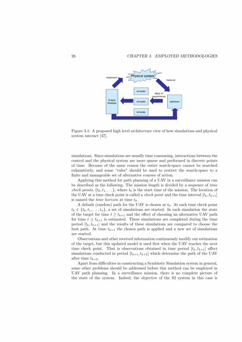
A proposed high level architecture of how simulations and the physical systeminteract is depicted in Figure 3.1. The use of Symbiotic Simulation in managementof a semiconductor assembly and test facility has been studied e.g. in [48, 49]. Theuse of S2 in model-building for social sciences is discussed in [50].
The idea of Symbiotic Simulation obviously has similarities with control systemsand the loop depicted in Figure 3.1 resembles the feedback loop in an automaticcontroller. However, there are some characteristics that identify an S2 system. Inan S2 system the evaluation of input changes are not performed analytically but by
25
26 CHAPTER 3. EMPLOYED METHODOLOGIES
Figure 3.1: A proposed high level architecture view of how simulations and physicalsystem interact [47].
simulations. Since simulations are usually time consuming, interactions between thecontrol and the physical system are more sparse and performed in discrete pointsof time. Because of the same reason the entire search-space cannot be searchedexhaustively, and some “rules” should be used to restrict the search-space to afinite and manageable set of alternative courses of action.
Applying this method for path planning of a UAV in a surveillance mission canbe described as the following. The mission length is divided by a sequence of timecheck points, {t0, t1, . . . }, where t0 is the start time of the mission. The location ofthe UAV at a time check point is called a check point and the time interval [tk, tk+1]is named the time horizon at time tk.
A default (random) path for the UAV is chosen at t0. At each time check pointtk ∈ {t0, t1, . . . , tn}, a set of simulations are started. In each simulation the stateof the target for time t ≥ tk+1 and the effect of choosing an alternative UAV pathfor time t ≥ tk+1 is estimated. These simulations are completed during the timeperiod [tk, tk+1] and the results of these simulations are compared to choose thebest path. At time tk+1 the chosen path is applied and a new set of simulationsare started.
Observations and other received information continuously modify our estimationof the target, but this updated model is used first when the UAV reaches the nexttime check point. That is observations obtained in time period [tk, tk+1] affectsimulations conducted in period [tk+1, tk+2] which determine the path of the UAVafter time tk+2.
Apart from difficulties in constructing a Symbiotic Simulation system in general,some other problems should be addressed before this method can be employed inUAV path planning. In a surveillance mission, there is no complete picture ofthe state of the system. Indeed, the objective of the S2 system in this case is

3.2. PARTICLE FILTERING 27
to optimize the process of acquiring information. The sensor data, before thetarget is detected, consists mostly of “negative” information i.e. lack of sensormeasurement where it was (with some probability) expected [51]. This informationshould be utilized to modify our estimation of the target’s location. The processof drawing conclusions from sensor data is a problem studied by the informationfusion community. One powerful estimation technique used in information fusionis Sequential Monte Carlo (SMC) methods also known as Particle Filtering whichis based on point mass (or particle) representation of probability densities [52].Indeed, in tracking applications, SMC is an on-line simulation process, which runsin parallel with the data collection process and can be considered as some kind ofSymbiotic Simulation system, albeit it does not affect the physical system.
In on-line UAV path planning we use SMC to estimate the state of the target.This estimation (particle set) which is our only picture of the reality and is updatedcontinuously is used in “what-if” simulations to determine how the UAV shouldmove to collect new data as effectively as possible. This S2 path planning algorithmconsists of two parts. The first part is a main loop running in real-time in whichinformation is collected and our picture of the state of the system is updated.The other part is a set of “what-if” simulations that are initiated and executedperiodically and after reaching time check points. These simulations run fasterthan real-time and are executed concurrently. Comparing these simulation outputsdetermines the best course of action. The result can either be applied directly tothe system or used for decision support by a decision maker.
3.2 Particle Filtering
Particle Filtering (Sequential Monte Carlo methods) is a well-studied approachin data fusion and signal processing communities and is an appropriate tool forestimating the state of a non-linear system with a non-Gaussian process noise, usinga sequence of noisy measurements [53]. Particle Filtering is an iterative methodwhich repeatedly estimates the new state of the system according to a transitionmodel (propagation stage) and filters this result using a sensor model when newmeasurements are available (updating stage). Since measurements are assumed tobe available at discrete times, a discrete-time approach is convenient.
Introducing the time series t = {t0, t1, . . . }, the value of the time dependentvariable φ(t) at time t = tk is denoted by φk. The denotation φ0:k is the set ofall values {φ0, φ1, . . . , φk}. Using this notation the transition model, p(xk | xk−1),gives the conditional probability of the state xk given xk−1 and the sensor model,p(zk | xk), gives the conditional probability of observation zk, given the state xk.We are usually interested in the conditional state of the system, given the sequenceof observations z1:k, i.e. p(xk | z1:k). In general, this Probability Density Function(PDF), may be obtained recursively in two stages, prediction and update. The
28 CHAPTER 3. EMPLOYED METHODOLOGIES
prediction is calculated before the last observation zk is available
p(xk | z1:k−1) =∫
p(xk | xk−1, z1:k−1)p(xk−1 | z1:k−1)dxk−1
=∫
p(xk | xk−1)p(xk−1 | z1:k−1)dxk−1.
(3.1)
The first equality follows from p(xk) =∫
p(xk | xk−1)p(xk−1)dxk−1 and the secondequality is a result of the fact that the process is Markovian, i.e. given the currentstate, old observations have no effect on the future state [52].
In the update stage the conditional probability p(xk | z1:k) is calculated usingthe prediction result p(xk | z1:k−1) and the sensor model p(zk | xk) and when thelatest observation zk becomes available. In this step Bayes’ rule and Markov prop-erty are used.
p(xk | z1:k) =p(z1:k | xk)p(xk)
p(z1:k)=
p(zk, z1:k−1 | xk)p(xk)p(zk, z1:k−1)
=p(zk | xk, z1:k−1)p(z1:k−1 | xk)p(xk)
p(zk | z1:k−1)p(z1:k−1)=
p(zk | xk)p(z1:k−1 | xk)p(xk)p(zk | z1:k−1)p(z1:k−1)
=p(zk | xk)p(xk | z1:k−1)p(z1:k−1)
p(zk | z1:k−1)p(z1:k−1)=
p(zk | xk)p(xk | z1:k−1)p(zk | z1:k−1)
The first equality is Bayes’ theorem. The second equality uses the defini-tion z1:k = {zk, z1:k−1}. In the third equality definition of the conditional prob-ability is used. The fourth equality is the result of the Markov property, i.e.p(zk | xk, z1:k−1) = p(zk | xk). In the fifth equality Bayes’ rule is used again andfinally the sixth equality is just simplifying the quotient by p(z1:k−1). This resultis called update stage and is as follows:
p(xk | z1:k) =p(zk | xk)p(xk | z1:k−1)
p(zk | z1:k−1)(3.2)
where the denominator is calculated using
p(zk | z1:k−1) =∫
p(zk | xk)p(xk | z1:k−1)dxk. (3.3)
The recurrence relations 3.1 and 3.2 form the basis for the optimal solution,however, this set of recursive equations is only a conceptual solution since in generalit cannot be determined analytically. If the transition model and the sensor modelare linear and the process noise has a Gaussian distribution, which is a ratherrestrictive constraint, these calculations can be performed analytically by usingKalman Filters. When the analytical solution is intractable approximate methodssuch as Particle Filtering can be used [52].

3.2. PARTICLE FILTERING 29
A convenient method to represent a probability density function and its changesover time is to represent the density function by a set of random samples withassociated weights and to compute estimates based on these samples and weights.As the number of samples become very large, this Monte Carlo characterizationbecomes equivalent to the usual functional description of the probability densityfunction [52].
In Particle Filtering the probability density function of the target having thestate x, in each time-step tk is represented as a set of n particles pi
k = {(xik, wi
k)}ni=1,where xi
k is a point in the state-space and wik is the weight associated with this
point at time t = tk. These weights are non-negative and sum to unity. The lo-cation and weight of each particle reflect the value of the density in that regionof the state space. The Particle Filtering updates the particle locations and thecorresponding weights recursively with each new observation [54]. Particle Filter-ing starts with sampling a set of n particles, S0 = {(xi
0, wi0)}ni=1 from the given
distribution p(x0), such that the number of particles in each interval [a, b] is pro-portional to
∫ b
ap(x0)dx0. The weights of the particles are set equally to 1/n. At
each iteration, particles in the set Sk−1 are propagated using the transition model,that is by sampling from
p(xik | xi
k−1).
When new observations arrive the weights are updated according to
wik ∝ wi
k−1p(zk | xik)
where zk is the observation at time t = tk and p(z | x), is the sensor model. Particlesare resampled periodically considering their weights, i.e. they will be sampled withreplacement in proportion to their weights and weights are set to wi
k = 1/n. Thisstep is necessary to replicate particles with large weights and eliminate particleswith low weights and avoid degeneracy of the algorithm [52].
One natural application area of SMC methods is in surveillance and trackingapplications. The transition model is then derived from properties of the target,terrain characteristics and other forehand information we have about the mission ofthe target. The sensor model depends on the characteristics of the sensors and thesignature of the target. Many examples of applying Particle Filtering in surveillanceare provided in [53] and [55]. Examples of using Particle Filtering in terrain-aidedtracking is found in [55]. Application of Particle Filtering in sensor management issuggested in [44, 45].
To demonstrate how the Particle Filtering works in practice, we present brieflyhow we have implemented it in this thesis. Here we assume that a single targetis moving on a known road network. Some a priori information about the initiallocation of the target, an approximation of its velocity and some assumption aboutits goal is available. The Particle Filtering includes the following stages.

30 CHAPTER 3. EMPLOYED METHODOLOGIES
Sampling
Particle Filtering starts with sampling S0 = {(xi0, w
i0)}Ni=1 randomly from the a
priori information p(x0), such that the number of particles on each (small) roadsegment is proportional to the probability of existence of the target on that roadsegment. Each particle is assigned a velocity randomly sampled from the distri-bution of the target’s velocity and the weight of each particle is set equally to1/N .
Prediction
At iteration k, particles in the set Sk−1 are propagated forward, that is the newstate of the particles are calculated using their current location, velocity and aprocess noise based on the transition model, p(xk | xk−1). Since the motion of theparticles (vehicle) are bound to a known road network, their state can be specifiedby three variables. That is, xk = [rk, dk, vk], where rk is the current road segment,dk is the distance the particle has moved on road rk and vk is the instantaneousspeed of the particle.
Update
After the propagation the weights of the particles are modified depending on thesensor model and current sensor observation. A sensor signal in a point increasesthe importance (weights) of the particles near that point. On the contrary, lack ofsensor signals decreases the weights of the particles which are near the sensor. Forinstance if we have a perfect sensor and the UAV flies over a road segment and nosensor signal is supplied, the weights of all particles in that road segment are set tozero. After modifying the weights, they are normalized by dividing by the sum ofthe weights.
Resampling
A common problem with Particle Filtering is the degeneracy phenomenon whichrefers to the fact that after many iterations, the number of particles with negligibleweight increases and a large computational effort is devoted to updating particleswhose contribution to p(xk | zk) is almost zero. One method to reduce the effectof degeneracy is to resample particles, i.e. to eliminate particles that have smallweights and concentrate on particles with large weights. The resampling algorithmgenerates a new set of particles by sampling (with replacement) N times from theCumulative Distribution Function (CDF) of weights of particles. The weights ofthese new particles are assigned the value 1/N .

3.2. PARTICLE FILTERING 31
Summary
Symbiotic Simulation and Particle Filtering form the basis for the algorithms wehave used to address the UAV path planning problem. Details of these algorithmsare described in the papers in Part II.

Chapter 4
Contribution of the thesis
This chapter gives a short description of three papers, which reflect the main con-tributions of this thesis and are included in the second part of it. Thesis authorcontributions in each paper is also explained.
4.1 A Brief Summary of Published Papers
Papers published in conference proceedings are as follows:
Paper 1
Farzad Kamrani, Marianela Garcia Lozano, and Rassul Ayani. Path Planning forUAVs Using Symbiotic Simulation. In Proceedings of the 20th annual EuropeanSimulation and Modelling Conference, ESM’2006, Toulouse, France, October 2006.
This paper describes the general idea of using Symbiotic Simulation as a methodfor path planning of UAVs and introduces a framework for applying this methodon path planning of a UAV searching for a single ground target moving on a knownroad network. It is assumed that some uncertain a priori information about thetarget and its intention is available. By employing this information, the future stateof the target is simulated and the best course of action (path) for the UAV is chosenfrom a set of candidate actions. Since the scenario is only partially observable, anddynamic, the estimation of the future is not complete and is updated when new(sensor) information becomes available. Thus running the simulation in real-timeand in interaction with the system is an essential part of the solution (SymbioticSimulation).
To verify whether this method is feasible and to supply a tool to comparedifferent methods a special purpose simulation tool, called the S2-simulator wasdeveloped. This simulator and its features are presented in this paper.
33
34 CHAPTER 4. CONTRIBUTION OF THE THESIS
Thesis Author Contributions
The thesis author suggested the idea of using Symbiotic Simulation in path planningof UAVs and developed a framework for employing this method. Applying ParticleFiltering to estimate the location of the target on the road network and design andimplementation of the S2-simulator was performed by the thesis author.
Paper 2
Farzad Kamrani and Rassul Ayani. Simulation-aided Path Planning of UAV. Toappear in Proceedings of the Winter Simulation Conference, WSC’07, Washington,D.C., December 2007.
This paper focuses on the same problem as the previous paper and describestwo methods of searching a road network for a single target by a UAV. First anexhaustive search method which searches the entire road network in a manner thatguarantees to find the target (albeit after a long time) is presented. The mainobjective of this method is to establish necessary conditions for solvability of theproblem and serve as a reference for other methods. The second approach is asimulation based method which estimates the location of the target and focuses thesearch on road segments with higher probability of existence of the target. Howeverit is anticipated that the available model of the movements of the target does notchange during the mission. Hence, the simulations are performed prior to the startof the search operation and thus the UAV path is static and once calculated it isnot possible to modify it. The UAV follows the path until it either tracks the targetor reports a failure; indicating the target has not been detected after a specifiedtime. When comparing different UAV paths, the UAV path that minimizes theexpectation time of detecting the target is chosen.
To evaluate the performance of the off-line simulation-aided solution, a testscenario is designed and simulations are performed using the special purpose sim-ulation tool introduced in [56]. Different paths for the target are chosen and theefficiency of the exhaustive search and off-line simulation method are tested underequal conditions. The detection time obtained by these two methods is the measureof interest and compared.
Thesis Author Contributions
The thesis author suggested and designed the algorithms for the exhaustive searchand off-line simulation-aided path planning. He also suggested and designed atest case scenario for testing the performance of the methods, implemented thealgorithms using the S2-simulator, and performed the test and evaluation of themethods.

4.2. CONCLUSION AND FUTURE WORK 35
Paper 3
Farzad Kamrani and Rassul Ayani. Using On-line Simulation for Adaptive PathPlanning of UAVs. In Proceedings of the 11-th IEEE International Symposium onDistributed Simulation and Real Time Applications, Chania, Crete Island, Greece,October 2007.
In this paper the on-line simulation method, which was suggested in the firstpaper in general terms is studied in details. Given an estimation of the target’sposition the future position of the target is simulated. Based on this estimation,“What-if” simulations are conducted periodically and the consequences of choosingdifferent alternative paths are compared in coarse discrete time points. In eachtime step the path that decreases the uncertainty about the location of the targetis chosen. Hence, the expectation of information entropy as a measure for comparingdifferent courses of action of UAVs is introduced and employed in the algorithms.A UAV path that has a lower expectation of information entropy is preferable. Theperformance of the on-line simulation with the two methods described earlier in thesecond paper, i.e. off-line simulation-aided path planning and the exhaustive searchmethod is compared under equal conditions by simulating these three methods ona test case scenario using the S2-simulator.
Thesis Author Contributions
The thesis author designed the algorithms for the on-line simulation-aided pathplanning. The idea of using the expectation of the information entropy as a measureto compare different UAV paths was suggested by the thesis author and the relatedalgorithms were designed and implemented. A test case scenario for testing andcomparing the performance of the exhaustive search, off-line simulation, and on-linesimulation methods were also designed by the thesis author.
4.2 Conclusion and Future Work
The focus of this thesis is on simulation-based path planning of UAVs in search/findand search/surveillance missions. Since search operations are generally dynamic aSymbiotic Simulation that employs the latest available information is suggested. Asearch operation that utilizes the available a priori information, terrain data andreasonable assumptions about the target performs generally better than a uniformsearch. To fuse this uncertain information, Particle Filtering is used. The resultof the simulations on a simulator shows the feasibility of the method, and a rela-tively high performance. However, these tests are performed on a simulator usinga simplified model of the terrain, target and the UAV. It should also be noted thatthere is no guarantee that by using the Symbiotic Simulation, the detection timeof the target is always shorter than other methods, for instance a uniform search.The method only provides the possibility to adapt the actions to the informationmodel available and gives a higher probability of success.

36 CHAPTER 4. CONTRIBUTION OF THE THESIS
There are still many interesting questions to be answered and much more tobe done. We employed a simple heuristic method to define the alternative UAVpaths. Designing more effective algorithms that reduce the search space providesthe possibility to repeat the what-if simulations more often and obtaining a betterresult. One could claim that the quality of the search depends highly on the detailof the objective function and number of particles. However, research in these areasis needed to test these hypotheses.
Applying the method in more complex scenarios is also a natural continuationof this work. The complexity of a scenario may be due to the composition oftargets, number of UAVs or more complex terrain models. For instance multi-targets including different types which have a correlated movement and follow amission are significantly more difficult to model. Another interesting problem arisesif the scenario is more dynamic, e.g. if the target reacts depending on the chosenUAV path. All these extensions introduce new challenges in this area.
Bibliography
[1] Office of the Secretary of Defense. Unmanned Aircraft Systems (UAS)Roadmap, 2005-2030. Technical report, August 2005.
[2] Department of Defense. Dictionary of Military and Associated Terms, April2001.
[3] Office of the Secretary of Defense. Unmanned Aerial Vehicles (UAV) Roadmap,2002-2027. Technical report, December 2002.
[4] Greg Goebel. Unmanned Aerial Vehicles, April 2006. Available viahttp://www.vectorsite.net/twuav.html [accessed October 12, 2007].
[5] Laurance R. "Nuke" Necome. Unmanned Aviation, A Brief History of Un-manned Aerial Vehicles. American Institute of Aeronautics and Astronautics(AIAA), Reston, Virginia, USA, 2004.
[6] Bill Yenne. Attack of the Drones, A History of Unmanned Aerial Combat.Zenith press, St. Paul, Minnesota, USA, 2004.
[7] Remote Piloted Aerial Vehicles: An Anthology, 2003. Available viahttp://www.ctie.monash.edu/hargrave/rpav_home.html [accessed August 17,2007].
[8] Union Army Balloon Corps, From Wikipedia, the free encyclopedia. Availablevia http://en.wikipedia.org/wiki/Union_Army_Balloon_Corps [accessed Oc-tober 31, 2007].
[9] Ben B. Balsley, Michael L. Jensen, and Rod G. Frehlich. The Use of State-of-the-art Kites for Profiling the Lower Atmosphere. Boundary-Layer Meteorol-ogy, 87(1):1–25, April 1998.
[10] Charles J. Cohen. Early History of Remote Sensing. In Proceeding of AppliedImagery Pattern Recognition Workshop, pages 3–9, 2000.
[11] National Museum of the United States Air Force. Available viahttp://www.nationalmuseum.af.mil/ [accessed August 22, 2007].
37
38 BIBLIOGRAPHY
[12] Ryan Firebee, From Wikipedia, the free encyclopedia. Available viahttp://en.wikipedia.org/wiki/Ryan_Firebee [accessed August 23, 2007].
[13] ADM-20 Quail, From Wikipedia, the free encyclopedia. Available viahttp://en.wikipedia.org/wiki/ADM-20_Quail [accessed August 23, 2007].
[14] Ryan Model 147 Lightning Bug , From Wikipedia, the free encyclopedia. Avail-able via http://en.wikipedia.org/wiki/Ryan_Model_147_Lightning_Bug [ac-cessed August 23, 2007].
[15] W. Brown, J. Mims, and N. Heenan. An Experimental Microwave-PoweredHelicopter. In Proceeding of IRE International Convention Record, volume 13,pages 225–235, Mars 1965.
[16] J.O. McSpadden, F.E. Little, M.B. Duke, and A. Ignatiev. An In-space Wire-less Energy Transmission Experiment. In Proceeding of Energy ConversionEngineering Conference, volume 1, pages 468–473, August 1996.
[17] GA-ASI’s Predator UAS Series Achieves 300,000 Flight Hours, 2007. Avail-able via http://www.ga-asi.com/news_events/index.php [accessed August 31,2007].
[18] DARPA Completes Autonomous Airborne Refueling Demonstration, August2007. Available via http://www.spacewar.com [accessed August 14, 2007].
[19] Timothy H. Cox, Christopher J. Nagy, Mark A. Skoog, and Ivan A.Somers.Civil UAV Capability Assessment, 2004.
[20] Mitch Ferry, Ziming Tu, Leesa Stephens, and Graham Prickett. Towards TrueUAV Autonomy. In Proceeding of the Information, Decision and Control, pages170–175, February 2007.
[21] Bruce T. Clough. Metrics, Schmetrics! How The Heck Do You Determine AUAV’s Autonomy Anyway? In Proceedings of the 2002 PerMIS Workshop.NIST Special Publication 990, August 2002.
[22] Thomas M. Spura, Jerry L. Franke, Robert J. Szczerba, and Mike Scarangella.Command and Control of Unmanned Vehicles - where are we going? AmericanHelicopter Society 60th Annual Forum, June 2004.
[23] First Flight - True UAV Autonomy At Last, July 2004. Availablevia http://www.agent-software.com/shared/profile/expertise.html [accessedSeptember 11, 2007].
[24] Pete Schaefer, Richard D. Colgren, Richard J. Abbott, Han Park, Amir Fijany,Forest Fisher, Mark L. James, Steve Chien, Ryan Mackey, Michail Zak, Timo-thy L. Johnson, and Stephen F. Bush. Technologies for Reliable AutonomousControl (TRAC) of UAVs. In Proceedings of the 19th Digital Avionics SystemsConference (DASC), volume 1, pages 1E3/1–1E3/7, October 2000.
39
[25] M. Jun and R. D’Andrea. Path Planning for Unmanned Aerial Vehicles inUncertain and Adversarial Environments, volume 1 of Cooperative Systems,chapter 6, pages 95–111. Springer, 2002.
[26] S. M. LaValle. Planning Algorithms. Cambridge University Press, Cambridge,U.K., 2006. Also available at http://planning.cs.uiuc.edu/.
[27] P. Skoglar, J. Nygårds, R. Björström, P. Ögren, J. Hamberg, P. Hermansson,and M. Ulvklo. Path and Sensor Planning Framework Applicable to UAVSurveillance with EO/IR Sensors. Technical report, FOI-Swedish Defence Re-search Agency, SE-581 11 Linköping, Sweden, September 2005.
[28] Jonas Nygårds, Per Skoglar, Jörgen Karlholm, Rickard Björström, and MorganUlvklo. Towards Concurrent Sensor and Path Planning: A Survey of Plan-ning Methods Applicable to UAV Surveillance. Technical report, FOI-SwedishDefence Research Agency, SE-581 11 Linköping, Sweden, May 2005.
[29] I.K. Nikolos and A.N. Brintaki. Coordinated UAV Path Planning Using Dif-ferential Evolution. In Proceedings of the 2005 IEEE International Symposiumon, Mediterrean Conference on Control and Automation, pages 549– 556, 2005.
[30] B.J. Capozzi. Evolution-based Path Planning and Management for Au-tonomous Vehicles. PhD thesis, University of Washington, 2001.
[31] C. Hocaoglu and A.C. Sanderson. Planning Multiple Paths with EvolutionarySpeciation. IEEE Transactions on Evolutionary Computation, 5(3):169–191,Jun 2001.
[32] Anawat Pongpunwattana, Richard Wise, Rolf Rysdyk, and Anthony J. Kang.Multi-Vehicle Cooperative Control Flight Test. In Proceedings of the 25thDigital Avionics Systems Conference, 2006 IEEE/AIAA, pages 1–11, October2006.
[33] C. Fonlupt, D. Robilliard, and Ph. Preux. Preventing Premature Convergencevia Cooperating Genetic Algorithms. In Proceedings of the Mandel’97, Brno,Czech, June 1997.
[34] D. Jia and J. Vagners. Parallel Evolutionary Algorithms for UAV Path Plan-ning. In Proceedings of the AIAA 1st Intelligent Systems Technical Conference,Chicago IL, September 2004.
[35] C. Ippolito, G. Pisanich, and L.A. Young. Cognitive Emotion Layer Architec-ture for Intelligent UAV Planning, Behavior and Control. In Proceedings ofthe IEEE Aerospace Conference 2005, pages 1–16, March 2005.
[36] Lawrence D. Stone. What’s Happened in Search Theory since the 1975 Lanch-ester Prize? Operations Research, 37(3):501–506, May - June 1989.
40 BIBLIOGRAPHY
[37] Philip M. Morse. In Memoriam: Bernard Osgood Koopman, 1900-1981. Op-erations Research, 30(3):417–427, May - June 1982.
[38] Henry R. Richardson and Joseph H. Discenza. The United States Coast GuardComputer-Assisted Search Planning System (CASP). Naval Research LogisticsQuarterly, 27(4):659–680, March - April 1980.
[39] Lawrence D. Stone. The Process of Search Planning: Current Approachesand Continuing Problems. Operations Research, 31(2):207–233, March - April1983.
[40] F. Bourgault, T. Furukawa, and H.F. Durrant-Whyte. Optimal Search fora Lost Target in a Bayesian World. In Proceedings of the 4th InternationalConference on Field and Service Robotics (FSR’03), volume 24, pages 209–222, Lake Yamanaka, Japan, July 2003.
[41] Frédéric Bourgault, Tomonari Furukawa, and Hugh F. Durrant-Whyte. Coor-dinated Decentralized Search for a Lost Target in a Bayesian World. In Pro-ceedings of the 2003 IEEE/RSJ International Conference on Intelligent Robotsand Systems, volume 1, pages 48–53, Las Vegas, Nevada, October 2003.
[42] Frédéric Bourgault, Ali Göktogan, Tomonari Furukawa, and Hugh F. Durrant-Whyte. Coordinated Search for a Lost Target in a Bayesian World. AdvancedRobotics, 18(10):979–1000, 2004.
[43] N. Xiong and P. Svensson. Multi-sensor management for information fusion:issues and approaches. Information Fusion, 3(2):163–186, 2002.
[44] Simon Ahlberg, Pontus Hörling, Karsten Jöred, Christian Mårtenson, GöranNeider, Johan Schubert, Hedvig Sidenbladh, Pontus Svenson, Per Svensson,Katarina Undén, and Johan Walter. The IFD03 information fusion demon-strator. In Proceedings of the Seventh International Conference on InformationFusion, volume II, pages 936–943, June 2004.
[45] Pontus Svenson and Christian Mårtenson. SB-Plan: Simulation-based supportfor resource allocation and mission planning. In Proceedings of the Conferenceon Civil and Military Readiness (CIMI 2006), Enköping, Sweden, May 16–18,2006.
[46] Frederica Darema. Symbiotic Measurement and Simulation Application Sys-tems. In AI, Simulation and Planning in High Autonomy Systems, March2000.
[47] Richard Fujimoto, Dell Lunceford, Ernest Page, and Adelinde M. Uhrmacher.Summary of the Parallel/Distributed Simulation Working Group. In RichardFujimoto, Dell Lunceford, Ernest Page, and Adelinde M. Uhrmacher, editors,Grand Challenges for Modeling and Simulation, Dagstuhl Report, pages 49–52,August 2002.

41
[48] Malcolm Yoke Hean Low, Kong Wei Lye, Peter Lendermann, Stephen JohnTurner, Reman Tat Wee Chim, and Surya Hadisaputra Leo. An agent-basedapproach for managing symbiotic simulation of semiconductor assembly andtest operation. In Proceedings of the fourth international joint conference onAutonomous agents and multiagent systems, pages 85–92, 2005.
[49] Peter Lendermann, Malcolm Yoke Hean Low, Boon Ping Gan, Nirupam Julka,Lai Peng Chan, Stephen J. Turner, Wentong Cai, Xiaoguang Wang, Loo HayLee, Terence Hung, Simon J.E. Taylor, Leon F. McGinnis, and Stephen Buck-ley. An Integrated and Adaptive Decision-Support Framework for High-TechManufacturing and Service Networks. In M. E. Kuhl, N. M. Steiger, F. B. Arm-strong, and J. A. Joines, editors, Proceedings of the 2005 Winter SimulationConference, 2005.
[50] Catriona Kennedy and Georgios Theodoropoulos. Adaptive Intelligent Mod-elling for the Social Sciences: Towards a Software Architecture. Technicalreport, University of Birmingham, School of Computer Science, October 2006.Available via http://www.cs.bham.ac.uk/research/projects/aimss/ [accessedSeptember 17, 2007].
[51] Wolfgang Koch. On ‘negative’ information in tracking and sensor data fusion:Discussion of selected examples. In Proceedings of the Seventh InternationalConference on Information Fusion, volume I, pages 91–98, June 2004.
[52] S. Arulampalam, S. Maskell, N. Gordon, and T. Clapp. A tutorial on ParticleFilters for on-line non-linear/non-gaussian bayesian tracking. IEEE Transac-tions on Signal Processing, 50(2):174–188, February 2002.
[53] Arnaud Doucet, Nando de Freitas, and Neil Gordon. Sequential Monte CarloMethods in Practice. Springer Verlag, 2001.
[54] Rickard Karlsson. Particle Filtering for Position and Tracking Application.PhD thesis, Linköping University, 2005.
[55] Branko Ristic, Sanjeev Arulampalam, and Neil Gordon. Beyond the KalmanFilter: Particle Filters for Tracking Applications. Artech House Series Pub-lishers, 2004.
[56] Farzad Kamrani, Marianela Garcia Lozano, and Rassul Ayani. Path plan-ning for UAVs using symbiotic simulation. In Proceedings of the 20th annualEuropean Simulation and Modelling Conference, ESM’2006, pages 215–238,October 2006.


Part II
Published Papers
43

Chapter 5
Paper 1
Path Planning for UAVs Using Symbiotic Simulation.In Proceedings of the 20th annual European Simulation and ModellingConference, Toulouse, France, October 23-25, 2006.
45


5.1. INTRODUCTION 47
Path Planning for UAVs Using Symbiotic Simulation
Farzad Kamrani Rassul AyaniRoyal Institute of Technology Royal Institute of TechnologySE-164 40 Stockholm, Sweden SE-164 40 Stockholm, Sweden
E-mail: [email protected] E-mail: [email protected]
Marianela Garcia LozanoSwedish Defence Research Agency
SE-164 90 Stockholm, SwedenE-mail: [email protected]
Abstract
The problem of efficient path planning for Unmanned Aerial Vehicles (UAV) witha surveillance mission in a dynamic environment can in some cases be solved usingSymbiotic Simulation (S2), i.e. an on-line simulation that interacts in real-timewith the UAV and chooses its path. Sequential Monte Carlo Simulation, knownalso as Particle Filtering (PF) is an instance of such a simulation.
In this paper we describe a methodology and an algorithm to use PF for efficientpath planning of a UAV which searches a road network for a target. To verifywhether this method is feasible and to supply a tool to compare different methodsa simulator is developed. This simulator and its features are presented in this paperas well.
5.1 Introduction
Interest for Unmanned Aerial Vehicle (UAV) systems in both civilian and militaryareas has shown a considerable growth in recent years. Despite diversity in thesystems the trend is moving toward increasing autonomy of the UAVs. For exam-ple, the United States Air Force Research Laboratory (AFRL) has introduced thenotion of Autonomous Control Level, and describes ten such levels, ranging fromremotely piloted vehicles to fully autonomous swarms of Unmanned Combat AerialVehicles [1]. Constructing a framework for highly autonomous UAVs is a demand-ing task that cannot be tackled using just one science discipline and technique.One natural way to handle this complexity is decomposition of the problem into ahierarchy of manageable sub-problems [2]. For instance, the aerodynamic control

48 CHAPTER 5. PAPER 1
of a platform and its long-term path planning belong to different levels of controlhierarchy and can be controlled by different subsystems. In this hierarchy we fo-cus on long-term path planning for UAVs. In a static scenario the long-term pathplanning is primarily deterministic and can be computed off-line [2]. However, in adynamic situation the long-term path should be re-planned in response to changesin the environment and incoming observation reports. Thus planning in this case,is an on-line process running in parallel with the physical system. Our workinghypothesis is that Symbiotic Simulation (S2) [3–5] yields an appropriate decisionsupport tool for efficient utilization of UAVs.
Problem Statement
The problem, in its most general form, can be formulated as the following. Givenan area of responsibility, a set of UAV-borne sensors with different attributes and aprior estimation of the position and capabilities of moving ground targets, the taskis to perform a surveillance mission with a minimal total cost. Several parameterslike the chosen paths, operational costs of involved UAVs, hostile threats and thevalue of acquired information determines the total cost of the mission.
Using a state-space approach to model a dynamic system, we use the followingnotations: x(t) is the state of the observed system in time t, that is a vector holdingall information about ground targets in time t. This vector is denoted by xi whenusing discrete-time formulation. We use x to refer to the function x(t) itself, i.e.the entire time-evolution of the observed system. Similarly the notations y, y(t) andyi are used to show the state of the UAV platforms and sensors carried by them.Observations made by the sensors are denoted by z, z(t) and zi.
With these notations, the problem can be defined as: given the time length of themission tk, initial state of the UAVs (sensors) y0, the initial estimation of the targetsp(x0) and a user-defined objective function f(y), search for arg max
y∈U
∫ tk
0f(y)dt.
The search space is U = {y1 × · · · × yn}, where n is the number of UAVs and yj
is a time dependent vector holding the position and other necessary states of UAVnumber j and sensors carried by it.
Choice of the objective function f is not a trivial task. However, since the goal ofthe mission is to track ground targets, we assume that rapidly acquired informationhas a high value and the importance of an observation decreases by time, i.e. weare looking after such y that gives rise to as much observation as early as possible.Make note that observation z apart from y depends on the unknown state x. Otherparameters can be linearly combined with this parameter to construct an objectivefunction that reflects the desire of the UAVs’ commander in a specific situation.
Even if path and flight constraints like continuity and differentiability and otherconstraints on y that reflect the properties of UAVs and sensors, bound the set ofall y functions and decrease the size of the set U , this problem is obviously nottractable. However, if we have some rules to choose a limited subset U ′ ⊂ U , thesealternatives can be compared and the best one can be chosen. These rules should
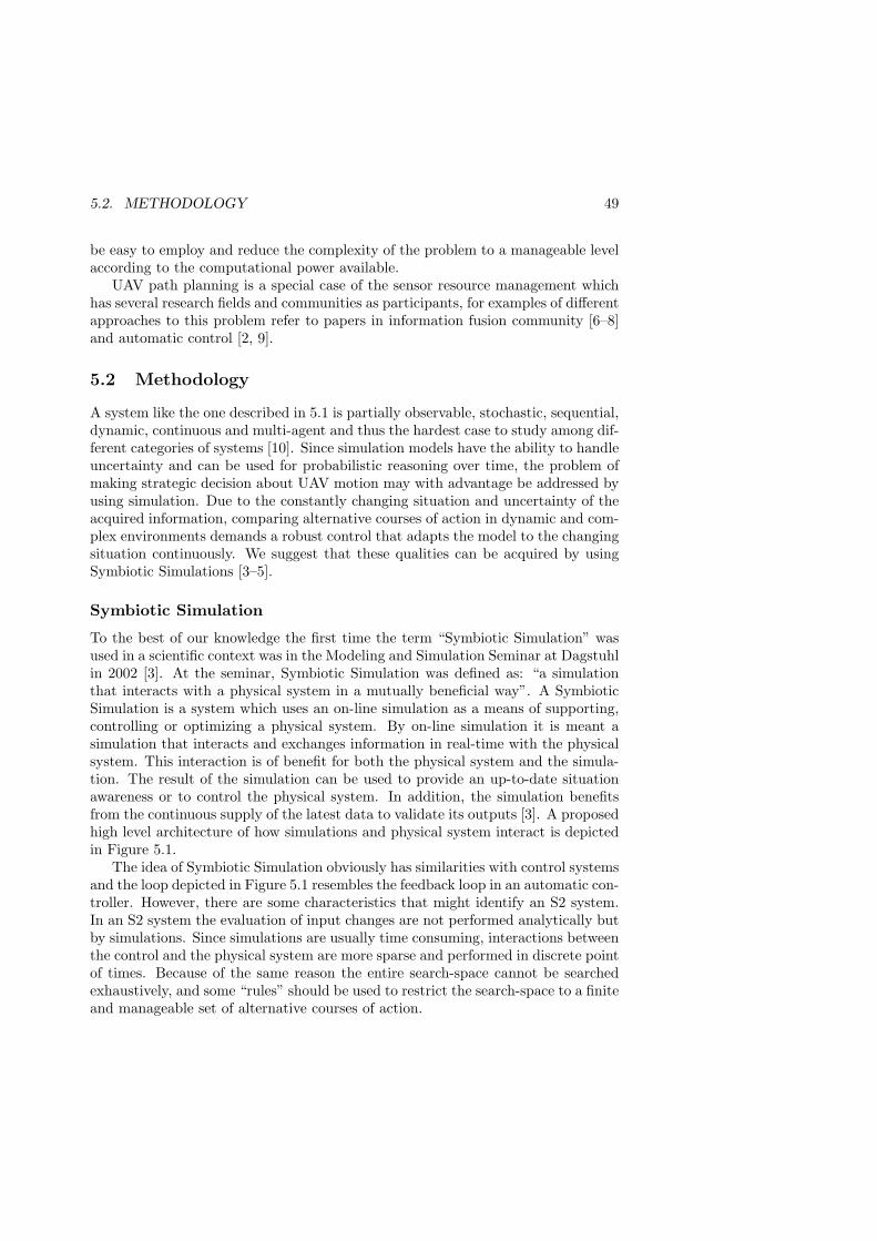
5.2. METHODOLOGY 49
be easy to employ and reduce the complexity of the problem to a manageable levelaccording to the computational power available.
UAV path planning is a special case of the sensor resource management whichhas several research fields and communities as participants, for examples of differentapproaches to this problem refer to papers in information fusion community [6–8]and automatic control [2, 9].
5.2 Methodology
A system like the one described in 5.1 is partially observable, stochastic, sequential,dynamic, continuous and multi-agent and thus the hardest case to study among dif-ferent categories of systems [10]. Since simulation models have the ability to handleuncertainty and can be used for probabilistic reasoning over time, the problem ofmaking strategic decision about UAV motion may with advantage be addressed byusing simulation. Due to the constantly changing situation and uncertainty of theacquired information, comparing alternative courses of action in dynamic and com-plex environments demands a robust control that adapts the model to the changingsituation continuously. We suggest that these qualities can be acquired by usingSymbiotic Simulations [3–5].
Symbiotic Simulation
To the best of our knowledge the first time the term “Symbiotic Simulation” wasused in a scientific context was in the Modeling and Simulation Seminar at Dagstuhlin 2002 [3]. At the seminar, Symbiotic Simulation was defined as: “a simulationthat interacts with a physical system in a mutually beneficial way”. A SymbioticSimulation is a system which uses an on-line simulation as a means of supporting,controlling or optimizing a physical system. By on-line simulation it is meant asimulation that interacts and exchanges information in real-time with the physicalsystem. This interaction is of benefit for both the physical system and the simula-tion. The result of the simulation can be used to provide an up-to-date situationawareness or to control the physical system. In addition, the simulation benefitsfrom the continuous supply of the latest data to validate its outputs [3]. A proposedhigh level architecture of how simulations and physical system interact is depictedin Figure 5.1.
The idea of Symbiotic Simulation obviously has similarities with control systemsand the loop depicted in Figure 5.1 resembles the feedback loop in an automatic con-troller. However, there are some characteristics that might identify an S2 system.In an S2 system the evaluation of input changes are not performed analytically butby simulations. Since simulations are usually time consuming, interactions betweenthe control and the physical system are more sparse and performed in discrete pointof times. Because of the same reason the entire search-space cannot be searchedexhaustively, and some “rules” should be used to restrict the search-space to a finiteand manageable set of alternative courses of action.
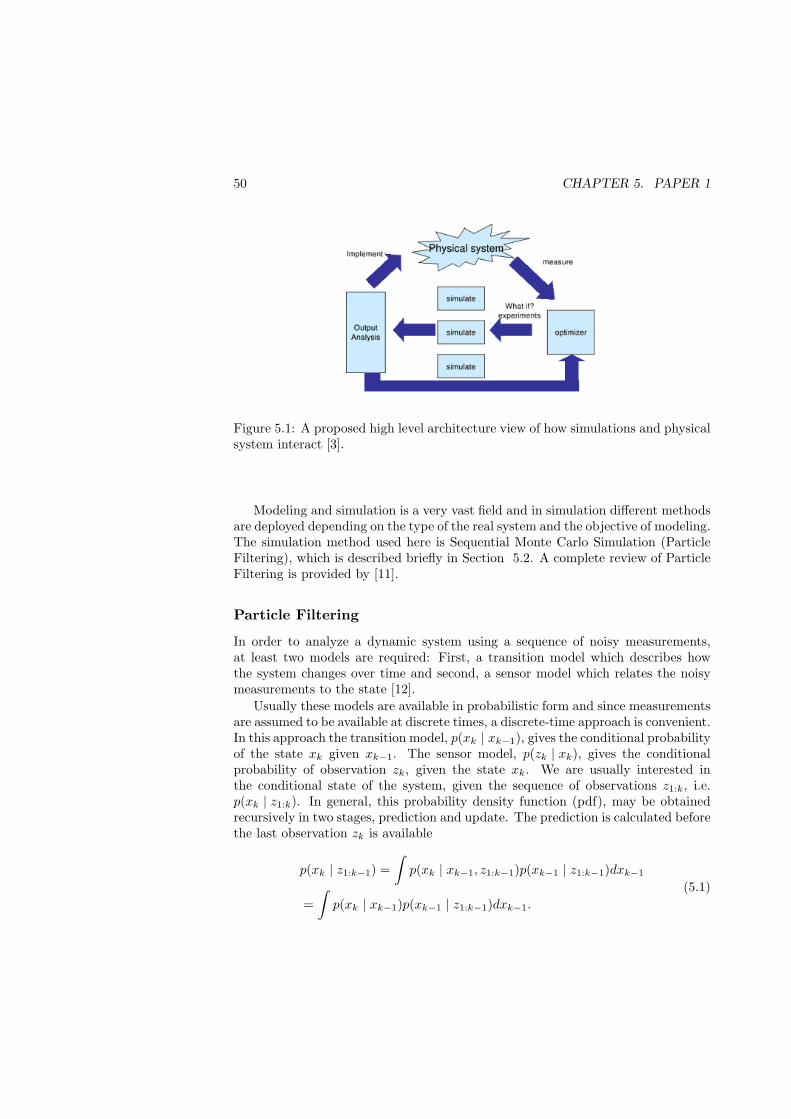
50 CHAPTER 5. PAPER 1
Figure 5.1: A proposed high level architecture view of how simulations and physicalsystem interact [3].
Modeling and simulation is a very vast field and in simulation different methodsare deployed depending on the type of the real system and the objective of modeling.The simulation method used here is Sequential Monte Carlo Simulation (ParticleFiltering), which is described briefly in Section 5.2. A complete review of ParticleFiltering is provided by [11].
Particle Filtering
In order to analyze a dynamic system using a sequence of noisy measurements,at least two models are required: First, a transition model which describes howthe system changes over time and second, a sensor model which relates the noisymeasurements to the state [12].
Usually these models are available in probabilistic form and since measurementsare assumed to be available at discrete times, a discrete-time approach is convenient.In this approach the transition model, p(xk | xk−1), gives the conditional probabilityof the state xk given xk−1. The sensor model, p(zk | xk), gives the conditionalprobability of observation zk, given the state xk. We are usually interested inthe conditional state of the system, given the sequence of observations z1:k, i.e.p(xk | z1:k). In general, this probability density function (pdf), may be obtainedrecursively in two stages, prediction and update. The prediction is calculated beforethe last observation zk is available
p(xk | z1:k−1) =∫
p(xk | xk−1, z1:k−1)p(xk−1 | z1:k−1)dxk−1
=∫
p(xk | xk−1)p(xk−1 | z1:k−1)dxk−1.
(5.1)
5.2. METHODOLOGY 51
The first equality follows from p(xk) =∫
p(xk | xk−1)p(xk−1)dxk−1 and the secondequality is a result of the fact that the process is Markovian, i.e. given the currentstate, old observations have no effect on the future state [12].
In the update stage the conditional probability p(xk | z1:k) is calculated usingthe prediction result when the latest observation zk becomes available via Bayes’rule
p(xk | z1:k) =p(zk | xk)p(xk | z1:k−1)
p(zk | z1:k−1)(5.2)
where the denominator is calculated using
p(zk | z1:k−1) =∫
p(zk | xk)p(xk | z1:k−1)dxk. (5.3)
If the transition model and the sensor model are linear and the process noise hasa Gaussian distribution, which is a rather restrictive constraint, these calculationscan be performed analytically by using Kalman Filter, otherwise some approximatemethod such as Particle Filtering (PF) should be used [12].
Sequential Monte Carlo Simulation (Particle Filtering) has been shown to be anappropriate tool for estimating the state of a non-linear system with a non-Gaussianprocess noise, using a sequence of noisy measurements. Intuitively, Particle Filter-ing is a Monte Carlo Simulation of how the state changes according to the transitionmodel, and to filter the result using the sensor model. Since the system changesover time, this process is repeated in parallel with the real system when new datais received. Even if new observations are not available the prediction stage still canbe used to predict the future state of the system. The procedure would be the samewith the exception that since future measurements are not known yet, the updatestage is not performed.
In particle filter the posterior pdf in each time-step k is represented as a set of npoints xi
k in the state-space and corresponding weights wik, i.e. pi
k = {(xik, wi
k)}ni=1,where pi
k is particle number i in time = k. The simulation begins with samplingS0, a set of n particles, from the prior distribution p(x0), such that
S0 = {(xi0, w
i0), w
i0 = 1/n}ni=1 (5.4)
and number of particles in each interval [a, b] is in proportion to∫ b
ap(x0)dx0.
At each iteration, particles in the set Sk−1 are updated using the transitionmodel, that is by sampling from
p(xik | xi
k−1) (5.5)
and when observations arrive the weights are recalculated using
wik ∝ wi
k−1p(zk | xik). (5.6)
Particles are resampled considering their weights, i.e. they will be sampled withreplacement in proportion to their weights and weights are set to wi
k = 1/n.
52 CHAPTER 5. PAPER 1
In a typical surveillance or tracking mission the objective is to estimate the stateof the system (position and velocity of the targets) as accurate as possible usinga sequence of noisy and uncertain observations received from some kind of sensorcarried by a platform (UAV). Particle Filtering and other methods (e.g. KalmanFilter, Extended Kalman Filter) have been extensively used to solve different in-stances of this problem. In these approaches the transition model describes thephysics of motion and the sensor model describes the measurement process.
Here we use the transition model to predict the future state of the system, anduse the sensor model to predict the future observations. These simulations are usedto search between various suggested UAV paths and choose the one that maximizesan objective function. These decisions are transfered to the control system of theUAV in check points. In these check points new “real” observations are transferedto the particle filter and resampling occurs.
5.3 S2-Simulator
In order to test and evaluate the idea of using S2 and Particle Filtering for long-termpath planning of UAVs in general and testing a special simplified case a simulationtool has been developed. The primary aim of this simulator, called S2-Simulator,is to provide a research tool for experimentation with different methods and tech-niques and provide indications about scalability and complexity of the algorithms.However in future it may well be developed and function as a prototype with morerealistic data. Some system attributes which have been in focus in developing S2-Simulator are simplicity, platform independence and flexibility. S2-Simulator isimplemented in Java programming language using object oriented technology.
The S2-Simulator is naturally divided into two parts: First, an emulation of thereal world including, terrain, target objects, their plans and UAVs and second, amodel of this “real” world that is used in S2-Simulations to improve the behaviorof the UAVs.
It should be clear that the information in the real world emulator is not availablein the second part, since the real world, e.g. the position and the plan of targets,should not be completely observable for UAV agents. However, for simplicity wecan assume that some part of UAVs perception from reality is exact, e.g. the mapof the terrain is accurate.
Terrain is modeled as a two-dimensional land and is composed of basic elementslike node, road, lake and forest. These elements are user-defined geometric shapesthat can easily be added to the terrain using a Graphical User Interface (GUI). Thereal-world view of the S2-Simulator which is used to generate scenarios is shown inFigure 5.2.
The probability of existence of targets of different types and the probabilitythat these targets are observed differ in these areas. That is the transition modeland the sensor model are dependent of the position in the terrain. Targets can beof different types, such as foot soldier, car, truck and tank. Targets have different
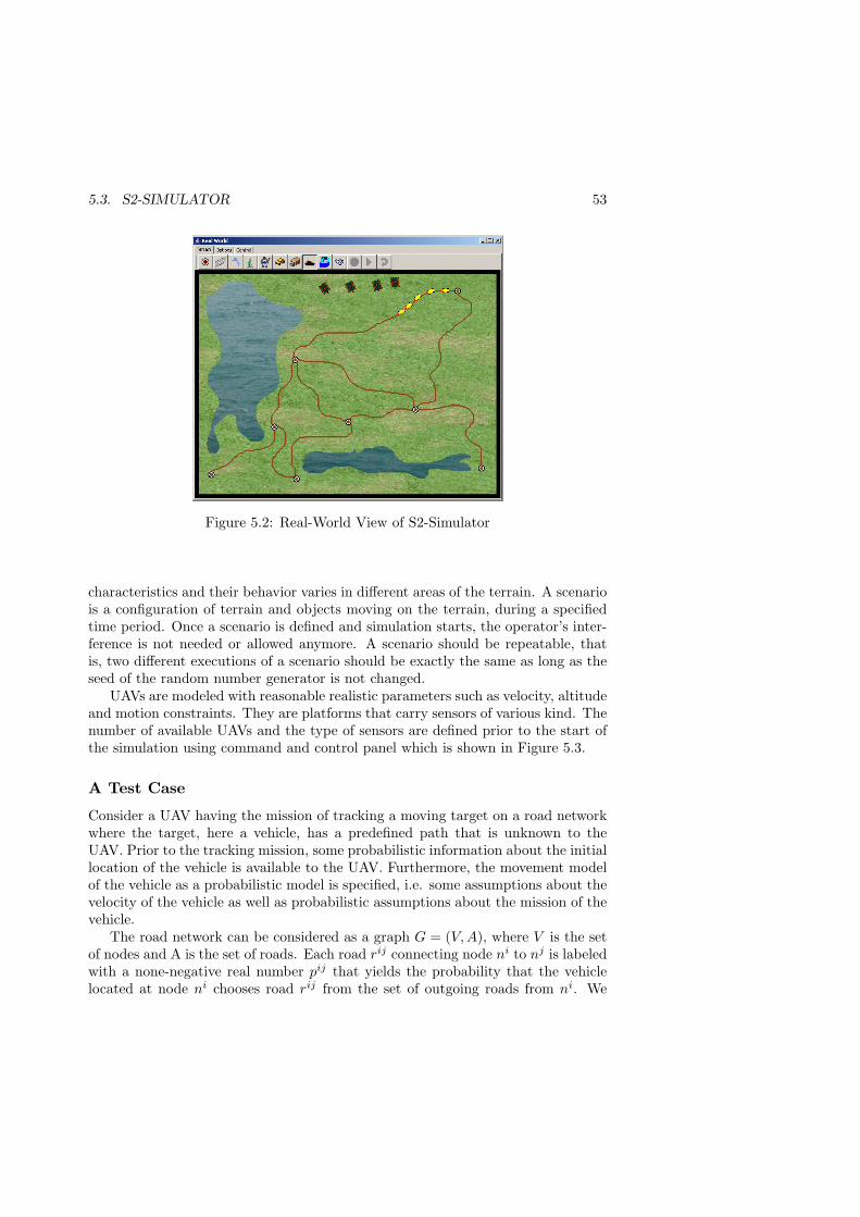
5.3. S2-SIMULATOR 53
Figure 5.2: Real-World View of S2-Simulator
characteristics and their behavior varies in different areas of the terrain. A scenariois a configuration of terrain and objects moving on the terrain, during a specifiedtime period. Once a scenario is defined and simulation starts, the operator’s inter-ference is not needed or allowed anymore. A scenario should be repeatable, thatis, two different executions of a scenario should be exactly the same as long as theseed of the random number generator is not changed.
UAVs are modeled with reasonable realistic parameters such as velocity, altitudeand motion constraints. They are platforms that carry sensors of various kind. Thenumber of available UAVs and the type of sensors are defined prior to the start ofthe simulation using command and control panel which is shown in Figure 5.3.
A Test Case
Consider a UAV having the mission of tracking a moving target on a road networkwhere the target, here a vehicle, has a predefined path that is unknown to theUAV. Prior to the tracking mission, some probabilistic information about the initiallocation of the vehicle is available to the UAV. Furthermore, the movement modelof the vehicle as a probabilistic model is specified, i.e. some assumptions about thevelocity of the vehicle as well as probabilistic assumptions about the mission of thevehicle.
The road network can be considered as a graph G = (V,A), where V is the setof nodes and A is the set of roads. Each road rij connecting node ni to nj is labeledwith a none-negative real number pij that yields the probability that the vehiclelocated at node ni chooses road rij from the set of outgoing roads from ni. We
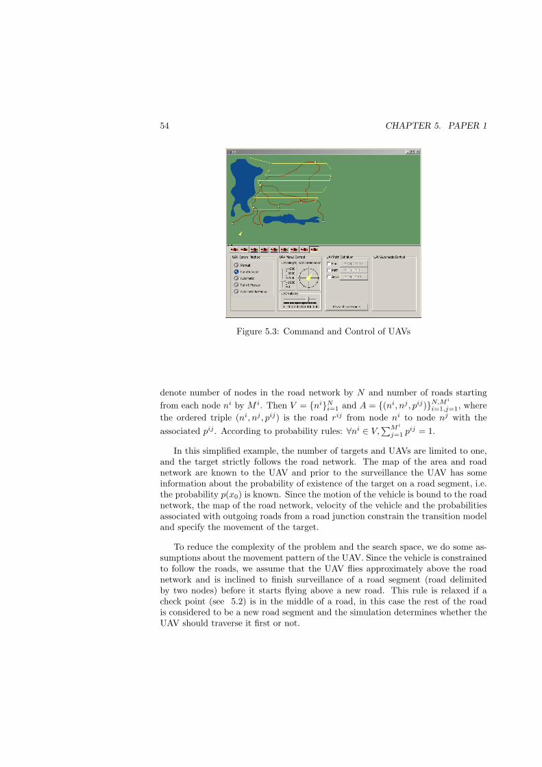
54 CHAPTER 5. PAPER 1
Figure 5.3: Command and Control of UAVs
denote number of nodes in the road network by N and number of roads startingfrom each node ni by M i. Then V = {ni}Ni=1 and A = {(ni, nj , pij)}N,Mi
i=1,j=1, wherethe ordered triple (ni, nj , pij) is the road rij from node ni to node nj with theassociated pij . According to probability rules: ∀ni ∈ V,
∑Mi
j=1 pij = 1.
In this simplified example, the number of targets and UAVs are limited to one,and the target strictly follows the road network. The map of the area and roadnetwork are known to the UAV and prior to the surveillance the UAV has someinformation about the probability of existence of the target on a road segment, i.e.the probability p(x0) is known. Since the motion of the vehicle is bound to the roadnetwork, the map of the road network, velocity of the vehicle and the probabilitiesassociated with outgoing roads from a road junction constrain the transition modeland specify the movement of the target.
To reduce the complexity of the problem and the search space, we do some as-sumptions about the movement pattern of the UAV. Since the vehicle is constrainedto follow the roads, we assume that the UAV flies approximately above the roadnetwork and is inclined to finish surveillance of a road segment (road delimitedby two nodes) before it starts flying above a new road. This rule is relaxed if acheck point (see 5.2) is in the middle of a road, in this case the rest of the roadis considered to be a new road segment and the simulation determines whether theUAV should traverse it first or not.

5.3. S2-SIMULATOR 55
Transition Model
The transition model which is a probabilistic model of the movement of targets isnot exact or complete. It is based on the assumption we have about type, propertyand goal of targets and information about the environment. The transition modelmay change during the mission, either as a direct result of new observations orunder the influence of external information e.g. analysis of the data in a higherlevel of data fusion. However, in this simplified example this possibility is ignoredand the transition model is a static model that does not change over time. The priorprobability p(x0) is a uniform (or another known) distribution over a road segment.The target has a specific type, with a maximum velocity and the distribution ofthe velocity is known.
We have a probabilistic assumption about the goal of the target, which in com-bination with the topology of the road network and quality of the roads can giveus the probability that the target follows each outgoing road when it arrives at acrossing. This information is sufficient to specify the transition model. The state-space of the target at time k is xk = [rk, dk, vk] where rk is the current road, dk
is the distance the target has moved on road rk and vk is the velocity of the tar-get. The noise vector is denoted by µk = [ξk, ρk], where ξk is velocity noise, andρk ∼ U [0, 1] is a random number which is used only when the target arrives at anode and reflects the uncertainty of the next chosen road segment by the target(lines 6 to 17 in Figure 5.4). If the target has not reached the end node of the road,it will stay on the same road segment (lines 4 and 5 in Figure 5.4). ∆t = tk+1 − tkis the time elapsed between two successive steps.
Sensor Model
The sensor model is generally described by the probabilistic model p(zk | xk), wherexk is the state of the system, and zk is the observation. The dimensions of the statezk are usually, but not necessarily, less than the dimensions of xk, since the systemis not completely observable. We choose to distinguish between the part of thesystem-state which is not under our control, i.e. the state of the target xk and thestate of the sensor yk. Hence the probabilistic sensor model would be p(zk | xk, yk).In our simplified example xk is specified by the three variables, as described in 5.3,which in combination with the terrain map clearly defines the location of the target.
We assume that the video interpretation task is solved by some means, i.e. wehave sensors that analyze the incoming video and alarm if they observe any target.Hence the state-space of the observation is binary and zk ∈ [ALARM,¬ALARM ].Inspired by [13] we suggest the following model for sensor observations at a standardheight.
p(ALARM | xk, yk) =
DP d ≤ δin
DP − (DP−FAP )(d−δin)δout−δin
δin ≤ d ≤ δout
FAP d ≥ δout
(5.7)

56 CHAPTER 5. PAPER 1
given: xk = [rk, dk, vk], µk = [ξk, ρk], G = (V,A),∆treturn: xk+1
1 propagate(xk, µk, G,∆t)2 dk+1 ← dk + vk∆t3 vk+1 ← vk + ξk
4 if dk+1 < length(rk)5 rk+1 ← rk
6 else7 cdf ← 08 ni ← end node of rk
9 R← extract {rij}Mi
j=1 from A10 while ρk < cdf11 rij ← choose rij with min pij from R12 R← R \ {rij}13 cdf ← cdf + pij
14 end while15 rk+1 ← rij
16 dk+1 ← dk+1 − length(rk)17 end if18 return [rk+1, dk+1, vk+1]19 end propagate
Figure 5.4: Transition Model
Where DP (detection probability), FAP (false alarm probability), δin and δoutare sensor specific and d is the two dimensional distance between the target and thevertical projection of the sensor on the earth, i.e. d =
√(xx
1 − xy1)2 + (xx
2 − xy2)2.
Changing the altitude of the UAV obviously influence the sensor model, but sincethe sensor model is not the focus of this paper, we assume that UAV has the samealtitude.
UAV Path Search
The outline of the algorithm of the main control loop of the UAV is depicted inFigure 5.6. Given a road network G and a UAV, the objective of this algorithmis to calculate periodically the best_known_path and move the UAV repeatedlyin time slice ∆t along this path. The loop terminates when the the mission timeis elapsed and the test at line 6 fails. A feasible chosen time period time_horizondivides the mission time to equally long time periods. These time periods de-termine check_points successively which are points that the UAV reaches after atime_horizon. A set of particles which always reflects our latest perception of thestate of the target is generated at line 4. This set is updated at line 18 when new

5.4. FUTURE WORK 57
6P (ALARM | d = δ)
-δ
1
DP
FAP
δin-�
δout -�
SS
SS
SS
SS
SS
SS
SS
SS
SS
SS
SS
SS
SS
SS
SS
Figure 5.5: Sensor Model
observations become available and propagated forward at line 19.A model of the UAV including its current state is created (at line 9). This model
and a copy of the particles are propagated forward a time_horizon at lines 11 and12. These propagations are our perception of the future. The estimated position ofthe UAV model after a time_horizon yields the next check_point at line 13 andthe untraversed part of the road network at line 14. These future states are thenpassed to the S2 simulation, which calculates the best path (line 15) for the UAVafter it has passed check_point.
The best_known_path is calculated by comparing the values of an objectivefunction for a finite set of paths by simulations. These paths are derived fromthe road network, e.g. by permutating the road segments and letting the UAVsurvey these roads in sequence (the UAV flies from the end of a road segment tothe beginning of the next road segment if these two points are not the same).
The details of the S2 algorithm and the Particle Filter used in the main loopas well as the tests performed will be presented in future papers. However, thepreliminary experiments indicate that a UAV supported by the S2 simulation issignificantly more efficient in tracking a target compared with a UAV that randomlysearches the road network.
5.4 Future Work
To complete this work, the first step would be to design tests and verify the resultsof preliminary experiments.
In the future, more complex scenarios will be studied. The complexity of ascenario may be due to the composition of targets, number of UAVs or more complexterrain models. For instance multi-targets including different types which have acorrelated movement and follow a mission are significantly more difficult to model.In the same way, if more than one UAV is involved in the tracking mission a morecomplicated model would be necessary.

58 CHAPTER 5. PAPER 1
1 main_loop(uav,G, ∆t)2 s2_result ← a random path derived from G3 check_point ← start position of uav4 {particlei}Ni=1 ← sample(N, p(x0))5 time← 06 while time < mission_time_length7 if (uav position = check_point)8 best_known_path = s2_result9 uav′ ← a model of the uav
10 {particle′i}Ni=1 ← copy of {particlei}Ni=0
11 move uav’ for time_horizon12 propagate {particle′i}Ni=0 in time_horizon13 check_point ← position of uav’14 G← G\traversed roads by uav′
15 s2_result← s2(G, uav′, {particle′i})16 end if17 z ← read sensors18 update all {particlei}Ni=1 using z19 propagate all {particlei}Ni=1 for ∆t20 move uav for ∆t along best_known_path21 time← time + ∆t22 end while23 end main_loop
Figure 5.6: Main Loop of the UAV
5.5 Conclusion
In this paper, we presented a framework for using Symbiotic Simulation in pathplanning of UAVs performing a surveillance mission. A special purpose simulatorwhich is developed to test whether this methodology is feasible was described, and ageneral structure of a simplified test case was outlined. Even though it is necessaryto systematically design and perform simulations before any reliable statementscould be made, preliminary experiments with the S2-Simulator are promising andindicate that S2 can be used for path planning of a UAV in a tracking mission.
5.6 Acknowledgment
This work is part of a project funded by the Swedish Defence Research Agency(FOI). We would like to thank Farshad Moradi, Pontus Svenson and Robert Suzićat FOI for their comments, suggestions and constructive critiques.
Bibliography
[1] Bruce T. Clough. Metrics, Schmetrics! How The Heck Do You Determine AUAV’s Autonomy Anyway? In Proceedings of the 2002 PerMIS Workshop.NIST Special Publication 990, August 2002.
[2] P. Skoglar, J. Nygårds, R. Björström, P. Ögren, J. Hamberg, P. Hermansson,and M. Ulvklo. Path and Sensor Planning Framework Applicable to UAVSurveillance with EO/IR Sensors. Technical report, FOI-Swedish Defence Re-search Agency, SE-581 11 Linköping, Sweden, September 2005.
[3] Richard Fujimoto, Dell Lunceford, Ernest Page, and Adelinde M. Uhrmacher.Summary of the Parallel/Distributed Simulation Working Group. In RichardFujimoto, Dell Lunceford, Ernest Page, and Adelinde M. Uhrmacher, editors,Grand Challenges for Modeling and Simulation, Dagstuhl Report, pages 49–52,August 2002.
[4] Malcolm Yoke Hean Low, Kong Wei Lye, Peter Lendermann, Stephen JohnTurner, Reman Tat Wee Chim, and Surya Hadisaputra Leo. An Agent-BasedApproach for Managing Symbiotic Simulation of Semiconductor Assembly andTest Operation. In AAMAS ’05: Proceedings of the fourth international jointconference on Autonomous agents and multiagent systems, pages 85–92, NewYork, NY, USA, 2005. ACM Press.
[5] Peter Lendermann, Malcolm Yoke Hean Low, Boon Ping Gan, Nirupam Julka,Lai Peng Chan, Stephen J. Turner, Wentong Cai, Xiaoguang Wang, Loo HayLee, Terence Hung, Simon J.E. Taylor, Leon F. McGinnis, and Stephen Buck-ley. An Integrated and Adaptive Decision-Support Framework for High-TechManufacturing and Service Networks. In M. E. Kuhl, N. M. Steiger, F. B. Arm-strong, and J. A. Joines, editors, Proceedings of the 2005 Winter SimulationConference, 2005.
[6] Pontus Svenson and Christian Mårtenson. SB-Plan: Simulation-Based Supportfor Resource Allocation and Mission Planning. In Proceedings of the Conferenceon Civil and Military Readiness (CIMI 2006), Enköping, Sweden, May 16–18,2006.
59
60 BIBLIOGRAPHY
[7] N. Xiong and P. Svensson. Multi-Sensor Management for Information Fusion:Issues and Approaches. Information Fusion, 3(2):163–186, 2002.
[8] Ronnie Johansson and Robert Suzić. Particle Filter-Based Information Acqui-sition for Robust Plan Recognition. In Proceedings of the Eighth InternationalConference on Information Fusion (FUSION 2005), Philadelphia, Pennsylva-nia, July 2005.
[9] Ben T. Ludington, Liang Tang, and George J. Vachtsevanos. Target Trackingin an Urban Warfare Environment Using Particle Filters. In Proceedings ofIEEE Aerospace Conference, Big Sky, MT, March 5–12, 2005.
[10] Stuart Russell and Peter Norvig. Artificial Intelligence A Modern Approach.Prentice Hall, second edition, 2003.
[11] Arnaud Doucet, Nando de Freitas, and Neil Gordon. Sequential Monte CarloMethods in Practice. Springer Verlag, 2001.
[12] S. Arulampalam, S. Maskell, N. Gordon, and T. Clapp. A Tutorial on Par-ticle Filters for On-line Non-linear/Non-Gaussian Bayesian Tracking. IEEETransactions on Signal Processing, 50(2):174–188, February 2002.
[13] J. Lichtenauer, M. Reinders, and E. Hendriks. Influence of the ObservationLikelihood Function on Particle Filtering Performance in Tracking Applica-tions. In Proceedings of the 6th International Conference on Automatic Faceand Gesture Recognition, 2004.

Chapter 6
Paper 2
Simulation-aided Path Planning of UAV.To appear in Proceedings of the 2007 Winter Simulation Conference,Washington, D.C., USA, December 9-12, 2007.
61

6.1. INTRODUCTION 63
Simulation-aided Path Planning of UAV
Farzad KamraniRassul Ayani
Royal Institute of Technology (KTH)School of Information and Communication Technology (ICT)
SE-164 40 Stockholm, [email protected]
Abstract
The problem of path planning for Unmanned Aerial Vehicles (UAV) with a trackingmission, when some a priori information about the targets and the environment isavailable can in some cases be addressed using simulation. Sequential Monte CarloSimulation can be used to assess the state of the system and target when the UAVreaches the area of responsibility and during the tracking task. This assessmentof the future is then used to compare the impact of choosing different alternativepaths on the expected value of the detection time. A path with a lower expectedvalue of detection time is preferred. In this paper the details of this method isdescribed. Simulations are performed by a special purpose simulation tool to showthe feasibility of this method and compare it with an exhaustive search.
6.1 Introduction
The focus in this article is on (long-term) path planning of UAVs in tracking mis-sions where some a priori information about the target and terrain topology isavailable. The a priori information about the target is assumed to be available inform of probabilistic measures (distributions). This information is based on reportsfrom other information sources and may include the initial probability distributionof the existence of the target, an assumption about the destination of the targetand an approximation of the target’s velocity. Moreover the terrain topology, inthis article a road network, which constrains the movement of the target is knownand a map of the terrain is available to the UAV system in digital format.
In this paper, we suggest using simulation to assess the state of the target inthe future and testing alternative UAV paths against this estimated future. These“what-if” simulations are performed in advance and before the UAV starts its

64 CHAPTER 6. PAPER 2
mission. The intuition behind this method is that utilizing information, even whenit is incomplete or uncertain, is essential in constructing effective search strategiesand a system that uses all pieces of information performs better compared withsystems not considering this information. In order to utilize this information werely on Modeling and Simulation techniques which have shown to be an invaluabletool handling complex and ’difficult-to-analyze’ systems.
To study this solution, a special-purposed simulation tool, called S2-Simulatorearlier developed [1] is used. A test case for testing this method and comparingit with an exhaustive search method is designed and simulations are performed toverify results.
Related Work
The problem of path planning of UAV in surveillance mission (sensor platform steer-ing) is a subclass of the more general problem of sensor resource management. [2]presents a review of multi-sensor management. The idea of using simulated futureto allocate sensors is described in [3]. Simulation-based planning for allocation ofsensor resources is discussed in [4]. The instance of the problem discussed in thispaper, relies heavily on terrain constraints (road network) implied on the target’smovement. Terrain information is highly non-linear, [5] discusses incorporating thisinformation within the terrain-aided tracking.
The approach in this paper differs from others in that the only informationused to assess the future state of the target, is the topology of the road networkand assumptions about the movement and goal of the target. Hence, the processof fusing sensor data to assess position of the target is completely omitted.
6.2 Problem Formulation
We present the following problem model. Consider a UAV having the mission oftracking a single mobile non-evading target on a known road network. With non-evading, we mean that the target, here a vehicle, has a predefined fixed path. Thispath is unknown to the UAV. We assume some probabilistic a priori informationabout the initial state of the vehicle, p(x0), is available. For instance, it maybe known that the target starts from a point uniformly distributed over a roadsegment or some road segments in a region. If the type of the target is known,a distribution over the initial speed of the target may be available, otherwise auniform distribution over a reasonable range is assumed. The target is constrainedto move on the road network.
The velocity of the UAV is considerably higher than the velocity of the target,and there is only one target to be tracked. Hence, once the target is detected it canbe followed by the UAV and the main measure of interest is the time required todiscover the target for the first time. For simplicity, it is assumed that the sensorused for tracking is a “perfect” sensor, which always detects the target if it is in
6.3. EXHAUSTIVE SEARCH 65
a predefined radius. Having a more realistic sensor model, most algorithms andconclusions presented here, remain nearly the same. However, the results of testsimulations would be poorer.
We use a discrete-time approach and denote the position and velocity (state) ofthe target at time t = k by xk. Since the motion of the vehicle is bound to a knownroad network, its state can be specified by three variables. That is, xk = [rk, dk, vk],where rk is the current road, dk is the distance the target has moved on road rk
and vk is the instantaneous speed of the vehicle. Furthermore, the state transitionmodel (the movement model of the vehicle) as a probabilistic model is specified,i.e. the conditional probability p(xk | xk−1) is known. This model specifies theconditional probability distribution of the state of the target at time xk, given thestate at time xk−1. The probability that the target follows each outgoing road whenit arrives at a crossing is part of this model.
The road network can be considered as a kind of directed graph G = (N,R),where N = {ni} is the set of all nodes and R = {rij} is the set of all directed roads.Each road rij that connects node ni to nj is a vector of points, containing sufficientnumber of points to specify the geometry of the road with reasonable resolution.That is, road rij is defined as a triple (ni, nj , < points >).
To reduce the complexity of the problem, we make some assumptions aboutthe movement pattern of the UAV. We assume that the UAV flies approximatelyabove the road network and is inclined to finish surveillance of a road segment (roaddelimited by two nodes) before it starts flying above a new road. This assumptionis more justified in presence of occlusion, for example in urban environments orroads surrounded by trees and buildings. The UAV has a fixed maximum velocityand a fixed altitude which provides the best detection capability.
With these conditions, the problem can be defined as searching a directed graphfor finding a moving object that moves in the direction of the edges. Care shouldbe taken not to confuse the problem of “searching a graph” discussed in this paperwith searching state in a state-graph. The graph discussed here is a spatial graphthat is physically searched.
6.3 Exhaustive Search
The problem in its most general form has no solution. If a target on a road networkis free to move, stop and change direction, even in a rather simple network, it maybe undetected forever. However, in the presence of some constraints on the roadnetwork and the target’s movement the problem is guaranteed to have solution.If the road network is a directed acyclic graph and the target is only allowed tomove in the direction of the roads or stop, the problem is solvable, i.e. there arealgorithms that finally find the target. We present here an example of such analgorithm.
A directed acyclic graph G = ({n}, {r}) is a directed graph such that for anynode n ∈ G, there is no nonempty directed path that starts and ends on n. In
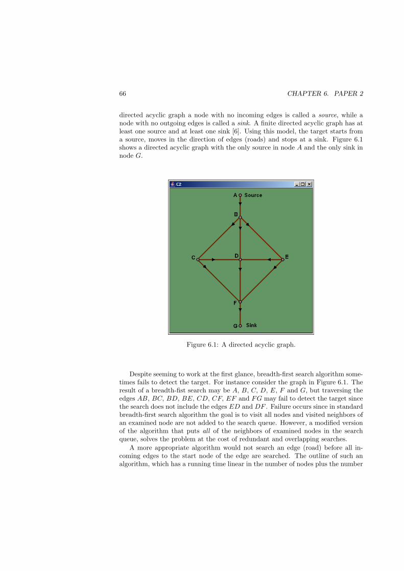
66 CHAPTER 6. PAPER 2
directed acyclic graph a node with no incoming edges is called a source, while anode with no outgoing edges is called a sink. A finite directed acyclic graph has atleast one source and at least one sink [6]. Using this model, the target starts froma source, moves in the direction of edges (roads) and stops at a sink. Figure 6.1shows a directed acyclic graph with the only source in node A and the only sink innode G.
Figure 6.1: A directed acyclic graph.
Despite seeming to work at the first glance, breadth-first search algorithm some-times fails to detect the target. For instance consider the graph in Figure 6.1. Theresult of a breadth-fist search may be A, B, C, D, E, F and G, but traversing theedges AB, BC, BD, BE, CD, CF, EF and FG may fail to detect the target sincethe search does not include the edges ED and DF . Failure occurs since in standardbreadth-first search algorithm the goal is to visit all nodes and visited neighbors ofan examined node are not added to the search queue. However, a modified versionof the algorithm that puts all of the neighbors of examined nodes in the searchqueue, solves the problem at the cost of redundant and overlapping searches.
A more appropriate algorithm would not search an edge (road) before all in-coming edges to the start node of the edge are searched. The outline of such analgorithm, which has a running time linear in the number of nodes plus the number

6.3. EXHAUSTIVE SEARCH 67
givendirected acyclic graph G = ({n}, {r})
start topological_sort(G)1 Q a First in First out queue2 Q← enqueue all nodes with no incoming roads3 while (Q is non-empty)4 n← dequeue Q5 for (each node m with a road from n to m)6 traverse the road rnm
7 if (target found)8 return9 end if
10 remove road rnm from the graph11 if (m has no other incoming roads)12 Q← enqueue m13 end if14 end for15 end while16 if (graph has roads)17 output error message (graph has a cycle)18 else19 no target was found20 end if
end topological_sort
Figure 6.2: Searching in topological order.
of edges is shown in Figure 6.2. This algorithm searches the graph in topologicalsorting.
A topological sort is a permutation p of the nodes of a graph such that an edge rij
implies that i appears before j in p. Only directed acyclic graph can be topologicallysorted [7]. As a consequence, if i appears before j in p, there is no path from jto i. Every directed acyclic graph has at least one topological sort, which may benot unique. For instance {A, B, C, E, D, F, G} and {A, B, E, C, D, F, G} are(the only) two topological sortings of the graph in Figure 6.1. The algorithm inFigure 6.2 orders the nodes in topological sorting and traverses edges that startfrom each of these nodes. This search always detects the target, since the searchis complete and according to the above, there is no path from the yet unsearchededges of the graph to those already searched. Failure to detect the target when thesearch is completed implies that the target has moved from the unsearched area tothe searched area, which is not possible.
As an example we apply this algorithm to the graph in Figure 6.1. The search

68 CHAPTER 6. PAPER 2
starts with enqueuing node A in a FIFO queue (Q), dequeuing it, traversing roadAB and enqueuing B. Then, node B is dequeued from Q, roads BC, BD and BEare traversed, but only nodes C and E are enqueued. Node D is not added toQ, since it has two more incoming edges, CD and ED. The algorithm continuesby dequeuing node C from Q, traversing roads CD and CF , dequeuing node E,traversing road ED, enqueuing node D and traversing road EF . Remaining stepsare dequeuing D, traversing road DF , enqueuing and dequeuing node F , travers-ing road FG and adding node G to Q. The algorithm terminates when node Gis removed from Q. In short, the roads are searched in the following order anddirection: AB, BC, BD, BE, CD, CF, ED, EF, DF and FG. The path of theUAV then is composed of traversing these roads in the given direction and order.The UAV moves from the end of a road to the start of the next if these two pointsare not the same.
Note that, in the algorithm in Figure 6.2, the structure Q does not need to be aFIFO queue and a set may be used instead. However, even if the topological sortingis preserved by using a set, in many cases, it results in an unbalanced search of thegraph. Even using a FIFO queue, the output of the algorithm in Figure 6.2 is notunique and it may be optimized by changing the order in which the outgoing roadsfrom a node are traversed (lines 5 and 6). It is sometimes possible to allow the UAVto move in the opposite direction of a road without compromising the correctness ofthe algorithm to obtain an even shorter path. For example, an optimization of theearlier given search order yields: AB, BC, DB, BE, ED, EF, FC, CD, DF andFG. The path using these road segments includes only two “extra” movementsfrom C to D and from D to E.
6.4 Our Aproach
We suggest prioritizing search in part of the road network where the probability ofthe existence of the target is higher. In order to locate these regions a Monte Carlomethod similar to Particle Filtering (also called Sequential Monte Carlo Simulation)is proposed, hence the name simulation-aided path planning.
Particle Filtering is a well-studied approach in data fusion and signal processingcommunities and is an appropriate tool for estimating the state of a non-linear sys-tem with a non-Gaussian process noise, using a sequence of noisy measurements [8].Particle filtering is an iterative method which repeatedly estimates the new stateof the system according to a transition model (propagation stage) and filters thisresult using a sensor model when new measurements are available (updating stage).Since measurements are assumed to be available at discrete times, a discrete-timeapproach is convenient.
In tracking, the transition model specifies the probability of location of thetarget at time t = tk, given its location at time t = tk−1. This model is derivedfrom properties of the target, terrain characteristics and other forehand informationwe have about the mission of the target. The sensor model is the probability of
6.4. OUR APROACH 69
existence of the target in a location, given an observation. The probability densityfunction of the target having the state x, in each time-step k is represented as a setof n particles pi
k = {(xik, wi
k)}ni=1, where xik is a point in the state-space and wi
k isthe weight associated with this point at time t = tk. These weights are non-negativeand sum to unity.
Particle filtering starts with sampling a set of n particles, S0 = {(xi0, w
i0)}ni=1
from the given distribution p(x0), such that the number of particles in each interval[a, b] is proportional to
∫ b
ap(x0)dx0. The weights of the particles are set equally to
1/n. At each iteration, particles in the set Sk−1 are propagated using the transitionmodel, that is by sampling from p(xi
k | xik−1). When new observations arrive the
weights are updated according to wik ∝ wi
k−1p(zk | xik) where, zk is the observation
in time t = k and p(z | x), is the sensor model. Particles are resampled periodicallyconsidering their weights, i.e. they will be sampled with replacement in proportionto their weights and weights are set to wi
k = 1/n. This step is necessary to replicateparticles with large weights and eliminate particles with low weights and avoiddegeneracy of the algorithm [9].
In simulation-aided path planning, the simulation of future is performed beforethe tracking mission is started. Due to the lack of any sensor information, theestimated state of the target is completely based on the transition model. Thisresults in a simpler model of particles without having any weights and makes theupdating and resampling stages unnecessary. The procedure would be the samewith the exception that since future measurements are not known yet, the updatingand resampling stages are omitted.
Once the future state of the target over a period of time is estimated, thisprediction is used to compare various suggested UAV paths and choose the onethat minimizes the expected value of the detection time. This path is static andonce calculated, it does not change during the mission and under the influence ofobservations. The UAV follows the path until it either tracks the target or reportsa failure; indicating the target has not been detected after adequate time.
How Does it Work?
Consider the rather simple road network in Figure 6.3. Assume that a movingobject is starting from point A and is moving towards one of the three goals E,F or G. The velocity of the object, vi, is one of the 25 discrete constant valuesvi ∈ {6, 7, 8, . . . , 30 m/s} with equal probability. When it reaches road junctionsB, C or D it takes one of the roads toward the goals with equal probability, i.e. thepath pj ∈ {ABCE, ABCF, ABDF, ABDG}. Having 25 possible different velocityvi and 4 different possible paths pj , there exists 25 ∗ 4 = 100 possible futures, eachequally probable.
A UAV has the mission to fly to this area of responsibility and locate the targetbefore it reaches one of the nodes E, F or G. The detection time τ is the criticalparameter that we want to minimize. We assume the UAV should fly over roadnetwork to detect the target and that the UAV traverses a road segment before
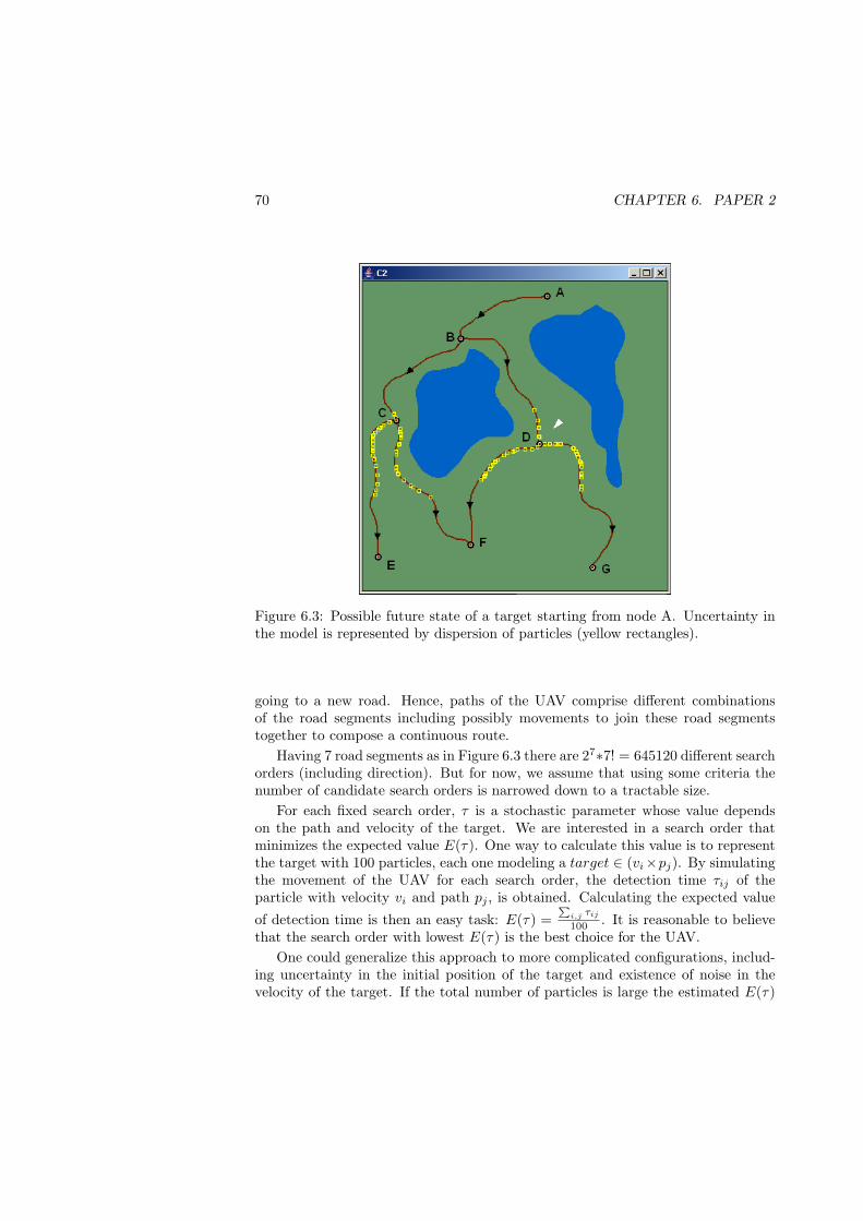
70 CHAPTER 6. PAPER 2
Figure 6.3: Possible future state of a target starting from node A. Uncertainty inthe model is represented by dispersion of particles (yellow rectangles).
going to a new road. Hence, paths of the UAV comprise different combinationsof the road segments including possibly movements to join these road segmentstogether to compose a continuous route.
Having 7 road segments as in Figure 6.3 there are 27∗7! = 645120 different searchorders (including direction). But for now, we assume that using some criteria thenumber of candidate search orders is narrowed down to a tractable size.
For each fixed search order, τ is a stochastic parameter whose value dependson the path and velocity of the target. We are interested in a search order thatminimizes the expected value E(τ). One way to calculate this value is to representthe target with 100 particles, each one modeling a target ∈ (vi×pj). By simulatingthe movement of the UAV for each search order, the detection time τij of theparticle with velocity vi and path pj , is obtained. Calculating the expected valueof detection time is then an easy task: E(τ) =
Pi,j τij
100 . It is reasonable to believethat the search order with lowest E(τ) is the best choice for the UAV.
One could generalize this approach to more complicated configurations, includ-ing uncertainty in the initial position of the target and existence of noise in thevelocity of the target. If the total number of particles is large the estimated E(τ)
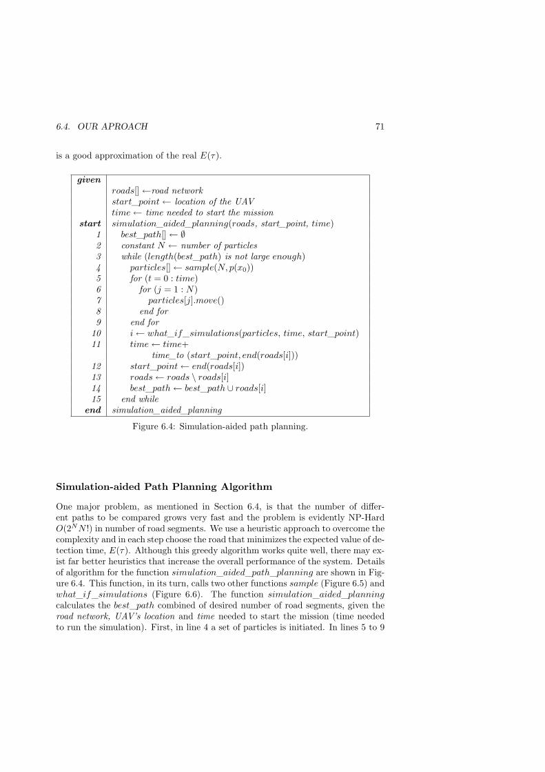
6.4. OUR APROACH 71
is a good approximation of the real E(τ).
givenroads[]←road networkstart_point← location of the UAVtime← time needed to start the mission
start simulation_aided_planning(roads, start_point, time)1 best_path[]← ∅2 constant N ← number of particles3 while (length(best_path) is not large enough)4 particles[]← sample(N, p(x0))5 for (t = 0 : time)6 for (j = 1 : N)7 particles[j].move()8 end for9 end for
10 i← what_if_simulations(particles, time, start_point)11 time← time+
time_to (start_point, end(roads[i]))12 start_point← end(roads[i])13 roads← roads \ roads[i]14 best_path← best_path ∪ roads[i]15 end while
end simulation_aided_planning
Figure 6.4: Simulation-aided path planning.
Simulation-aided Path Planning Algorithm
One major problem, as mentioned in Section 6.4, is that the number of differ-ent paths to be compared grows very fast and the problem is evidently NP-HardO(2NN !) in number of road segments. We use a heuristic approach to overcome thecomplexity and in each step choose the road that minimizes the expected value of de-tection time, E(τ). Although this greedy algorithm works quite well, there may ex-ist far better heuristics that increase the overall performance of the system. Detailsof algorithm for the function simulation_aided_path_planning are shown in Fig-ure 6.4. This function, in its turn, calls two other functions sample (Figure 6.5) andwhat_if_simulations (Figure 6.6). The function simulation_aided_planningcalculates the best_path combined of desired number of road segments, given theroad network, UAV’s location and time needed to start the mission (time neededto run the simulation). First, in line 4 a set of particles is initiated. In lines 5 to 9

72 CHAPTER 6. PAPER 2
givenp(x0) = [p(r0), p(d0), p(v0)]
start sample(p(x0))1 for(i = 1 : number_of_particles)2 r ← draw from p(r0)3 d← draw from p(d0)4 s← draw from p(v0)5 particle← a new particle6 set id of the particle to i7 set speed of the particle to s8 place the particle on the distance d of road r9 end for
end resample
Figure 6.5: Sampling Particles.
these particles are propagated forward to their estimated position by the time whenthe mission starts. This yields an approximation of the future state of the target.
Having an assessment of the future we can run a number of “what-if” simula-tions (in line 10) and calculate which alternative in the next period minimizes theexpected value of detection time.
The new start point of the UAV is set to the end of the chosen road in line 12and time is set to the time needed for the UAV to reach this point (line 11). Theroad chosen by the simulation is removed from roads vector in line 13 and addedto the best_path vector in line 14. The while loop controls if the best_path vectorhas the desired length in line 3.
To initiate a set of N particles according to a known a priori information, thefunction sample as defined in Figure 6.5 is called. We assume that the informationis given and expressed as a probability density function p(x0).
Since the state is defined by xk = [rk, dk, vk], it implies thatp(x0) = [p(r0), p(d0), p(v0)] is available, where p(r0) is the probability mass func-tion of the target being on a road. p(d0) is the probability density function ofthe target being on a distance from the start point of the road, and p(v0) is theprobability density function of the target having a velocity. Using these functions,we sample N particles from these distributions with replacement. Each particle isgiven a unique id number and is placed on a road. Similar to particle filtering, it isdifficult to make any precise statement on how many samples are required to give arepresentation of a probability function [10]. This number increases exponentiallywith the dimension of the state-space. We sample as many as we can computation-ally afford. In test programs in Section 6.5, the number of samples N , is equal to1000.
The algorithm for what-if simulations is given in Figure 6.6. In lines 3 to 7 as

6.4. OUR APROACH 73
globalobserved[nr_of_simulations][N ]← falseobservation_times[nr_of_simulations][N ]←∞
start what_if_simulations(particles, time, start_point)1 N ← number of particles2 nr_of_simulations← number of roads3 for (i = 1 : nr_of_simulations)4 u[i]← model of uav(start_point)5 u[i].set_mission(roads[i])6 simulation_done[i]← false7 end for8 tick ← 09 while (not all simulations completed)
10 for (k = 1 : N)11 particles[k].move()12 end for13 for (i = 1 : nr_of_simulations)14 if (not simulation_done[i])15 simulation_done[i]← u[i].move()16 for (k = 1 : N)17 if (‖(x, y)particles[k] − (x, y)u[i]‖ < ε)18 if(not observed[i][k])19 observed[i][k]← true20 observation_times[i][k]← time + tick21 end if22 end if23 end for24 end if25 end for26 tick ← tick + 127 end while28 min← arg min
i(PN
k=1 observation_times[i][k])/N
29 for (i = 1 : nr_of_simulations and k = 1 : N)30 observation_times[i][k]← observation_times[min][k]31 end for32 return min
end what_if_simulations
Figure 6.6: What-if Simulations.
many “What-if” simulations as the number of road segments are initiated. Thesesimulations are run to find the road segment that minimizes the expected value ofdetecting particles. The while loop in lines 9 to 27 continues until all these simula-tions are completed. In each step of this loop, all particles and all UAV models aremoved forward for a time unit. The return value of the UAV models’ move function
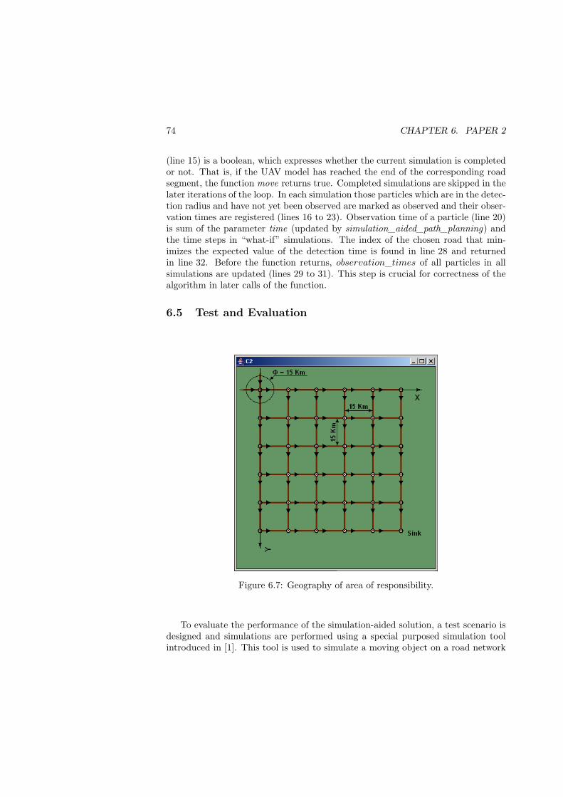
74 CHAPTER 6. PAPER 2
(line 15) is a boolean, which expresses whether the current simulation is completedor not. That is, if the UAV model has reached the end of the corresponding roadsegment, the function move returns true. Completed simulations are skipped in thelater iterations of the loop. In each simulation those particles which are in the detec-tion radius and have not yet been observed are marked as observed and their obser-vation times are registered (lines 16 to 23). Observation time of a particle (line 20)is sum of the parameter time (updated by simulation_aided_path_planning) andthe time steps in “what-if” simulations. The index of the chosen road that min-imizes the expected value of the detection time is found in line 28 and returnedin line 32. Before the function returns, observation_times of all particles in allsimulations are updated (lines 29 to 31). This step is crucial for correctness of thealgorithm in later calls of the function.
6.5 Test and Evaluation
Figure 6.7: Geography of area of responsibility.
To evaluate the performance of the simulation-aided solution, a test scenario isdesigned and simulations are performed using a special purposed simulation toolintroduced in [1]. This tool is used to simulate a moving object on a road network

6.5. TEST AND EVALUATION 75
and a UAV which has the mission to track this target. Different paths for the targetare chosen and the efficiency of the exhaustive search and simulation-aided searchmethods are tested under equal conditions. Detection times obtained for these twomethods are compared.
Figure 6.8: Detection time as a function of UAV’s distance to the origin in exhaus-tive search and simulation-aided search. Four different target paths are compared.
The geography of this scenario, as shown in Figure 6.7, consists of a regularroad network of perpendicular crossroads. Each road segment is 15 km long andthese 60 road segments make an area of responsibility that covers a square of size75 Km times 75 Km.
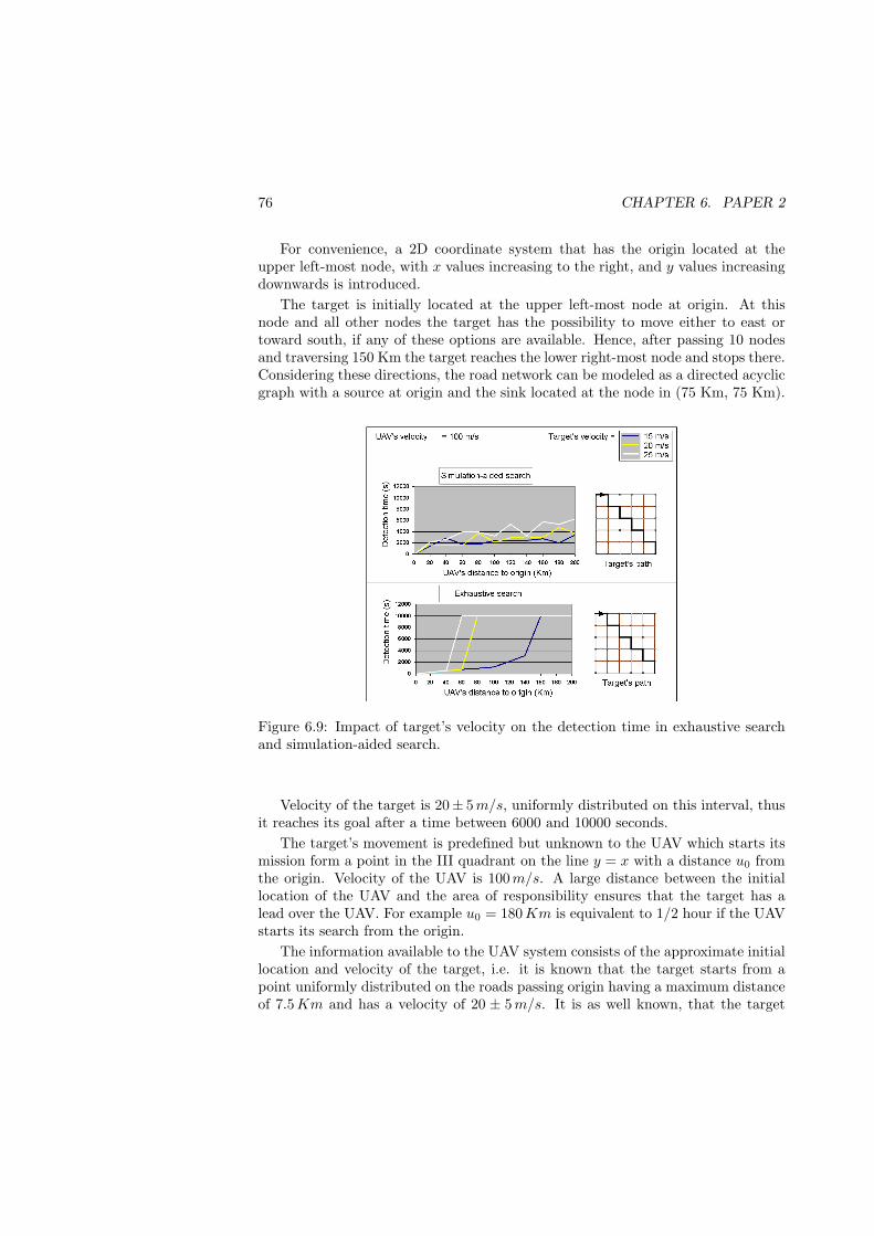
76 CHAPTER 6. PAPER 2
For convenience, a 2D coordinate system that has the origin located at theupper left-most node, with x values increasing to the right, and y values increasingdownwards is introduced.
The target is initially located at the upper left-most node at origin. At thisnode and all other nodes the target has the possibility to move either to east ortoward south, if any of these options are available. Hence, after passing 10 nodesand traversing 150 Km the target reaches the lower right-most node and stops there.Considering these directions, the road network can be modeled as a directed acyclicgraph with a source at origin and the sink located at the node in (75 Km, 75 Km).
Figure 6.9: Impact of target’s velocity on the detection time in exhaustive searchand simulation-aided search.
Velocity of the target is 20± 5 m/s, uniformly distributed on this interval, thusit reaches its goal after a time between 6000 and 10000 seconds.
The target’s movement is predefined but unknown to the UAV which starts itsmission form a point in the III quadrant on the line y = x with a distance u0 fromthe origin. Velocity of the UAV is 100 m/s. A large distance between the initiallocation of the UAV and the area of responsibility ensures that the target has alead over the UAV. For example u0 = 180Km is equivalent to 1/2 hour if the UAVstarts its search from the origin.
The information available to the UAV system consists of the approximate initiallocation and velocity of the target, i.e. it is known that the target starts from apoint uniformly distributed on the roads passing origin having a maximum distanceof 7.5 Km and has a velocity of 20 ± 5 m/s. It is as well known, that the target

6.5. TEST AND EVALUATION 77
chooses one of the outgoing roads (if more than one) downward or to the right andthere is no reason to believe that the target prefers one of these outgoing roads.
Considering all the constraints discussed, in addition to chosen search strategyof the UAV, there still remains three parameters that affect the detection time ofthe target: distance of the UAV to the area of responsibility, the target’s velocityand the target’s path. In order to compare the performance of the simulation-aided search and exhaustive search methods, simulations with different values ofthese three parameters in two main categories are conducted. In the first categorythe relation between the detection time and distance of the UAV to origin for 4different chosen paths by the target are studied. In the second category the impactof the target’s velocity on the detection time for one chosen path is studied. Theexhaustive search utilized here, is an optimized version of the search in topologicalorder of the roads as described in Figure 6.2. UAV’s path has been optimized tominimize extra movements between the end of a road segment and the start of thenext. The simulation-aided search algorithm needs 5 simulated minutes to simulate60 “what-if” simulations with 1000 particles in depth 16. That is, it composes apath for the UAV using 16 road segments. Simulations are run by time factor 10,i.e. 10 simulated seconds take 1 clock second. A modest computational power(a PC with 2 GHz processor and 1 GB RAM) has been used for this purpose. Toincrease our confidence in the results, all simulations are run 10 times using differentrandom seeds and the average values are presented.
In Figures 6.8 detection time of the target as a function of the distance of theUAV to the origin, for both methods and for 4 different target paths are depicted.The values on the horizontal axis show the distance u0 of the UAV to the origin,beginning from 0 to a maximum of 700 Km. The vertical axis shows the averagetime for detection of the target. In both search methods if the UAV fails to detectthe target in 10000 seconds, the search is stopped since this time is long enoughfor the target, even having lowest velocity, to reach its goal. As expected in all 4experiments, the detection time increases by increasing the distance of the UAVto the origin. While in the simulation-aided search method, the detection timeremains significantly under 10000 seconds for all values, in the exhaustive search itexceeds 10000 seconds rapidly. Summarizing these results, we can conclude that thesimulation-aided search method in most cases succeeds to detect the target beforeit reaches its goal while exhaustive search fails to detect the target when the UAV’sdistance to origin is more than 120 Km.
To study the effect of the velocity of the target on the detection time, 3 series oftests with different velocities for both search methods are conducted and the resultsare given in Figure 6.9. In both cases, velocities of the target are in the range 15to 25 m/s which is a range anticipated by the UAV. As expected, in both searchmethods, by increasing the velocity of the target, the detection time increases.However, in exhaustive search this increasing results in earlier failure of the mission(for shorter distance between the UAV and origin), but in simulation-aided searchthe detection time stays considerably under 10000 seconds.
78 CHAPTER 6. PAPER 2
6.6 Future Work
One of shortcoming of the simulation-aided approach as presented here is that thesimulations are run prior to the start of the mission. The path of the UAV iscalculated using an a priori model, which does not change during the mission inresponse to sensor data. In a simple scenario, where only one target is involved,and the objective is to detect the target for the first time before any sensor datais available, this method is feasible. However, in a more complex scenario, wherethe aim of the mission is to track several objects, a more dynamic path planningmethod is desirable. One way to address this problem is to run similar “what-if” simulations in real-time, i.e. under the entire surveillance mission. In thesereal-time simulations, the model and prediction of the future is refined by theincoming sensor data periodically. The simulations are repeated and the UAV’spath is changed dynamically. In future work, we will address real-time simulationsfor path planning of UAVs.
6.7 Conclusion
In this paper, we presented a method for path planning of a UAV with the task oftracking a moving target on a road network. This search method utilizes “what-if”simulations to prioritize the search in areas where the probability of existence ofthe target is higher.
An exhaustive search method that searches the road network in the direction ofthe movement of the target was also described. These two methods are compared byrunning simulations in a special-purposed simulation tool. Except for cases wherethe distance of the UAV to the origin is under 120 Km, simulation-aided approachshows superior results in detection time.
Acknowledgments
This work is part of a project funded by the Swedish Defence Research Agency(FOI). We would like to thank Pontus Svenson, Farshad Moradi and MarianelaGarcia Lozano at FOI for their comments, suggestions and constructive critiques.
Author Biography
Farzad Kamrani is a PHD student in the School of Information and Commu-nication Technology at Royal Institute of Technology (KTH), Stockholm, Sweden.He holds a Master of Science in Computer Science from Göteborg University. Hisresearch interests are simulation methodologies and Particle Filtering. His emailaddress is [email protected].
Rassul Ayani is professor of computer science in the School of Information and
6.7. CONCLUSION 79
Communication Technology at the Royal Institute of Technology (KTH), Stock-holm, Sweden. He received his first degree from University of Technology in Vienna(Austria), his MSc from University of Stockholm and his PhD from Royal Instituteof Technology (KTH) in Stockholm. Prof. Ayani has been conducting research ondistributed systems, distributed simulation and wireless networks since 1985. Hehas served as program chair and program committee members at numerous inter-national conferences and have been an associate editor of the ACM Transactions onModeling and Computer Simulation (TOMACS) since 1991. His web page can befound via http://www.it.kth.se/∼rassul. His email address is [email protected].

Bibliography
[1] Farzad Kamrani, Marianela Garcia Lozano, and Rassul Ayani. Path plan-ning for UAVs using symbiotic simulation. In Proceedings of the 20th annualEuropean Simulation and Modelling Conference, ESM’2006, pages 215–238,Toulouse, France, October 23–25, 2006.
[2] N. Xiong and P. Svensson. Multi-sensor management for information fusion:issues and approaches. Information Fusion, 3(2):163–186, 2002.
[3] Simon Ahlberg, Pontus Hörling, Karsten Jöred, Christian Mårtenson, GöranNeider, Johan Schubert, Hedvig Sidenbladh, Pontus Svenson, Per Svensson,Katarina Undén, and Johan Walter. The IFD03 information fusion demon-strator. In Proceedings of the Seventh International Conference on InformationFusion, volume II, pages 936–943, Mountain View, CA, Jun 2004.
[4] Pontus Svenson and Christian Mårtenson. SB-Plan: Simulation-based supportfor resource allocation and mission planning. In Proceedings of the Conferenceon Civil and Military Readiness (CIMI 2006), Enköping, Sweden, May 16–18,2006.
[5] Branko Ristic, Sanjeev Arulampalam, and Neil Gordon. Beyond the KalmanFilter: Particle Filters for Tracking Applications. Artech House Radar Library.Artech House Series Publishers, 2004.
[6] Eric W. Weisstein. Acyclic digraph, From Mathworld–A Wolfram web resource, 2003. Available viahttp://mathworld.wolfram.com/AcyclicDigraph.html [accessed March 29,2007].
[7] Eric W. Weisstein. Topological sort, From Mathworld–A Wolfram web resource, 2000. Available viahttp://mathworld.wolfram.com/TopologicalSort.html [accessed March 29,2007].
[8] Arnaud Doucet, Nando de Freitas, and Neil Gordon. Sequential Monte CarloMethods in Practice. Springer Verlag, 2001.
81

82 BIBLIOGRAPHY
[9] S. Arulampalam, S. Maskell, N. Gordon, and T. Clapp. A tutorial on particlefilters for on-line non-linear/non-gaussian bayesian tracking. IEEE Transac-tions on Signal Processing, 50(2):174–188, February 2002.
[10] N. J. Gordon, D. J. Salmond, and A. F. M. Smith. Novel approachto nonlinear/non-Gaussian Bayesian state estimation. IEE Proceedings-F,140(2):107–113, April 1993.

Chapter 7
Paper 3
Using On-line Simulation for Adaptive Path Planning of UAVs.In Proceedings of the 11-th IEEE International Symposium on Dis-tributed Simulation and Real Time Applications, Chania, Crete Island,Greece, October 22-24, 2007.
83


7.1. INTRODUCTION 85
Using On-line Simulation for Adaptive Path Planning of UAVs
Farzad KamraniRassul Ayani
Royal Institute of Technology (KTH)School of Information and Communication Technology (ICT)
SE-164 40 Stockholm, [email protected]
Abstract
In a surveillance mission, the task of Unmanned Aerial Vehicles (UAV) path plan-ning can in some cases be addressed using Sequential Monte Carlo (SMC) simu-lation. If sufficient a priori information about the target and the environment isavailable an assessment of the future state of the target is obtained by the SMCsimulation. This assessment is used in a set of “what-if” simulations to comparedifferent alternative UAV paths. In a static environment this simulation can be con-ducted prior to the mission. However, if the environment is dynamic, it is requiredto run the “what-if” simulations on-line i.e. in real-time.
In this paper the details of this on-line simulation approach in UAV path plan-ning is studied and its performance is compared with two other methods: an off-linesimulation-aided path planning and an exhaustive search method. The conductedsimulations indicate that the on-line simulation has generally a higher performancecompared with the two other methods.
7.1 Introduction
Path planning is a well-known term discussed in many domains and it refers torather different problems in different science communities. With UAV path plan-ning here we mean determining the path of the UAV so that it effectively can tracka target when some information about the environment and the target is available.
We present the following problem model. Consider a UAV having the mission oftracking a single mobile target on a known road network. We assume some proba-bilistic a priori information about the initial state of the vehicle, p(x0), is available.For instance, it may be known that the target starts from a point uniformly dis-tributed over a road segment or some road segments in a region. If the type of thetarget is known, a distribution over the initial speed of the target may be availableotherwise a uniform distribution over a reasonable range is assumed. The target isconstrained to move on the road network.
86 CHAPTER 7. PAPER 3
When the target reaches a junction in the road network, the probability thatit chooses each of these roads is specified using assumptions about the goal of thetarget or other information that might affect the target’s choice. If no informationis available the outgoing roads are assigned equal probability.
The velocity of the UAV is considerably higher than the velocity of the target,and there is only one target to be tracked. Hence, once the target is detected it canbe followed by the UAV. In other words the main measure of interest is the timerequired to discover the target for the first time. For simplicity, it is assumed thatthe sensor used for tracking is a “perfect” sensor, which always detect the target ifit has a less than pre-defined distance from the sensor. For a more realistic sensormodel, most algorithms and conclusions presented here, remain nearly the same.However, the results of test simulations would be poorer.
The road network can be considered as a directed graph G = (N,R), whereN = {ni} is the set of all nodes and R = {rij} is the set of all directed roads.Each road rij that connects node ni to nj is a vector of points, containing ’enough’number of points to specify the geometry of the road with reasonable resolution.That is, road rij is defined as a triple (ni, nj , < points >).
To reduce the complexity of the problem and the search space, we make someassumptions about the movement pattern of the UAV. We assume that the UAV fliesabove the road network and is inclined to finish surveillance of a road segment (roaddelimited by two nodes) before it starts flying above a new road. This assumptionis more justified in presence of occlusion, for example in urban environments orroads surrounded by trees and buildings. The UAV has a fixed maximum velocityand a fixed altitude which provides the best detection capability.
7.2 Path Planning Approaches
In [1] two methods for path planning of a UAV were suggested and compared. Thetwo methods were exhaustive search and (off-line) simulation-aided search whichwe rename shortly off-line simulation. Exhaustive search is a search in topologicalorder [2] of the graph and searches all the roads to find the target. The off-line sim-ulation is a Monte Carlo method that estimates the probability of existence of thetarget when the UAV reaches the area of responsibility and prioritizes the searchin areas where this probability is higher. The exhaustive search method is simplebut has a poor performance. The off-line simulation method shows considerablyhigher performance. However one disadvantage of this method as mentioned in [1]is that the system is not adaptive and cannot change the chosen path when newinformation or sensor observations are available. In order to overcome this prob-lem we suggest using symbiotic simulation (S2). In this paper the terms on-linesimulation and symbiotic simulation are interchangeably used.
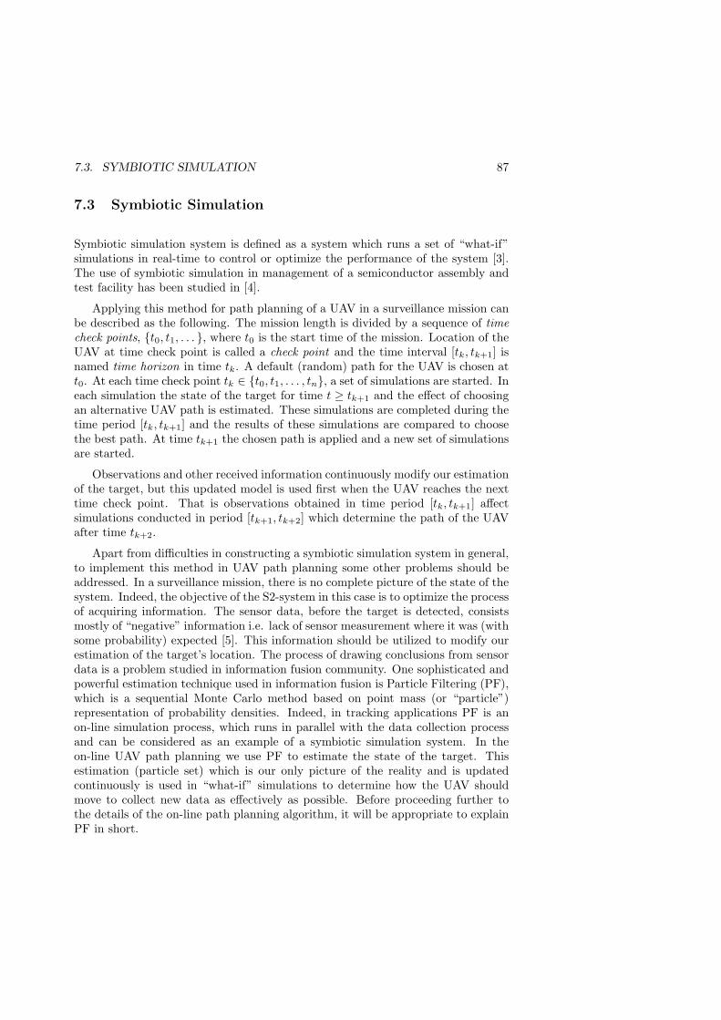
7.3. SYMBIOTIC SIMULATION 87
7.3 Symbiotic Simulation
Symbiotic simulation system is defined as a system which runs a set of “what-if”simulations in real-time to control or optimize the performance of the system [3].The use of symbiotic simulation in management of a semiconductor assembly andtest facility has been studied in [4].
Applying this method for path planning of a UAV in a surveillance mission canbe described as the following. The mission length is divided by a sequence of timecheck points, {t0, t1, . . . }, where t0 is the start time of the mission. Location of theUAV at time check point is called a check point and the time interval [tk, tk+1] isnamed time horizon in time tk. A default (random) path for the UAV is chosen att0. At each time check point tk ∈ {t0, t1, . . . , tn}, a set of simulations are started. Ineach simulation the state of the target for time t ≥ tk+1 and the effect of choosingan alternative UAV path is estimated. These simulations are completed during thetime period [tk, tk+1] and the results of these simulations are compared to choosethe best path. At time tk+1 the chosen path is applied and a new set of simulationsare started.
Observations and other received information continuously modify our estimationof the target, but this updated model is used first when the UAV reaches the nexttime check point. That is observations obtained in time period [tk, tk+1] affectsimulations conducted in period [tk+1, tk+2] which determine the path of the UAVafter time tk+2.
Apart from difficulties in constructing a symbiotic simulation system in general,to implement this method in UAV path planning some other problems should beaddressed. In a surveillance mission, there is no complete picture of the state of thesystem. Indeed, the objective of the S2-system in this case is to optimize the processof acquiring information. The sensor data, before the target is detected, consistsmostly of “negative” information i.e. lack of sensor measurement where it was (withsome probability) expected [5]. This information should be utilized to modify ourestimation of the target’s location. The process of drawing conclusions from sensordata is a problem studied in information fusion community. One sophisticated andpowerful estimation technique used in information fusion is Particle Filtering (PF),which is a sequential Monte Carlo method based on point mass (or “particle”)representation of probability densities. Indeed, in tracking applications PF is anon-line simulation process, which runs in parallel with the data collection processand can be considered as an example of a symbiotic simulation system. In theon-line UAV path planning we use PF to estimate the state of the target. Thisestimation (particle set) which is our only picture of the reality and is updatedcontinuously is used in “what-if” simulations to determine how the UAV shouldmove to collect new data as effectively as possible. Before proceeding further tothe details of the on-line path planning algorithm, it will be appropriate to explainPF in short.

88 CHAPTER 7. PAPER 3
Particle Filtering
For details of Particle Filtering, applications and the mathematical justification ofthe method refer to [6]. A tutorial on PF is provided by [7]. For examples ofusing PF in sensor management specially terrain-aided tracking [8] and [9] can beconsulted.
Here we explain the method intuitively and clarify how it is realized in ouralgorithm. A convenient method to represent a probability density function andits changes over time is to represent the density function by a set of random sam-ples with associated weights and to compute estimates based on these samples andweights. As the number of samples become very large, this Monte Carlo charac-terization becomes equivalent to the usual functional description of the probabilitydensity function [7].
Using a discrete time approach and introducing the time series t = {t0, t1, . . . },we denote the value of the time dependent variable φ(t) at time t = tk by φk. Thedenotation φ0:k is the set of all values {φ0, φ1, . . . , φk}.
Let Sk = {(xik, wi
k)}Ni=1 denote a set of N particles at time k, where each particleis a point xi
k in the state space and wik is a weight associated with this point. The
weights are normalized such that∑
i wik = 1.
Sampling: Particle Filtering starts with sampling S0 = {(xi0, w
i0)}Ni=1 randomly
from the a priori information p(x0), such that the number of particles on each(small) road segment is proportional to the probability of existence of the target onthat road segment. Each particle is assigned a velocity randomly sampled from thedistribution of the target’s velocity and the weight of each particle is set equally to1/N .
Prediction: At iteration k, particles in the set Sk−1 are propagated forward,that is the new state of the particles are calculated using their current location,velocity and a process noise. This model is called transition model, p(xk | xk−1).Since the motion of the particles (vehicle) are bound to a known road network,their state can be specified by three variables. That is, xk = [rk, dk, vk], where rk
is the current road segment, dk is the distance the particle has moved on road rk
and vk is the instantaneous speed of the particle.Update: After the propagation the weights of the particles are modified de-
pending on the sensor model and current sensor observation. A sensor signal in apoint increases the importance (weights) of the particles near that point. On thecontrary, lack of sensor signals decreases the weights of the particles which are nearthe sensor. For instance if we have a perfect sensor, weights of all particles in aroad segment are set to zero, if the UAV flies over the road segment and no sensorsignal is supplied. After modifying the weights, they are normalized by dividing bythe sum of the weights. Details of this algorithm is shown in Figure 7.1. In lines1 to 8, for each particle the distance of the particle and the sensor is calculated(line 2). If a sensor signal is received, the weight of the particle is multiplied by theprobability of registering a signal in this distance, p(ALARM | d). Otherwise, theweight is multiplied by 1− p(ALARM | d). In our tests we consider the sensor to

7.3. SYMBIOTIC SIMULATION 89
be a perfect sensor with the following model:
p(ALARM | d) =
{1 d ≤ 400 m
0 d > 400 m
The total weight of particles is calculated in line 9 and in lines 10 to 12 weights arenormalized.
giveny : location of the UAVparticles : {(xi
k, wik)}Ni=1
z : a sensor signalstart update_weights(particles, z, y)
1 for(i = 1 : N)2 d← distance( location of xi
k, y)3 if (z = ALARM)4 wi
k ← wikp(ALARM | d)
5 else6 wi
k ← wik(1− p(ALARM | d))
7 end if8 end for9 t←
∑Ni=1 wi
k
10 for(i = 1 : N)11 wi
k ← 1t w
ik
12 end for13 ˆNeff ← 1PN
i=1(wik)2
14 if ( ˆNeff < a threshold size )15 resample particles16 end if
end update_weights
Figure 7.1: Updating algorithm.
Resampling: A common problem with the PF is the degeneracy phenomenonwhich refers to the fact that after many iterations, the number of particles withnegligible weight increases and a large computational effort is devoted to updatingparticles whose contribution to p(xk | zk) is almost zero. One method to reduce theeffect of degeneracy is to resample particles, i.e. to eliminate particles that havesmall weights and concentrate on particles with large weights.
The resampling algorithm which is shown in Figure 7.2 generates a new set ofparticles by resampling (with replacement) N times from the cumulative distribu-tion function (cdf) of weights of particles. The weights of these new particles areassigned the value 1/N . In lines 1 to 4 this cdf is constructed. Then starting at

90 CHAPTER 7. PAPER 3
the bottom of the cdf a start point u1 is drawn uniformly from the interval [0, 1N ]
in line 6. In the loop in lines 7 to 14, N particles are drawn from the constructedcdf and their weights are assigned the value 1/N in line 13.
givenparticles : {(xi
k, wik)}Ni=1
start resample(particles)1 cdf [1]← w1
k
2 for(i = 2 : N)3 cdf [i]← cdf [i− 1] + wi
k
4 end for5 i← 16 u1 ← draw a starting point from U [0, 1
N ]7 for (j = 1 : N)8 uj ← u1 + j−1
N9 while (uj > cdf [i])
10 i← i + 111 end while12 xj
k ← xik
13 wjk ←
1N
14 end for15 return {(xj
k, wjk)}Nj=1
end resample
Figure 7.2: Resampling algorithm.
S2 Path Planning
The algorithm of path planning using symbiotic simulation is outlined in Figure 7.3.Given a road network, the initial location of the UAV and an a priori estimation ofthe location and velocity of the target, this algorithm runs “what-if” simulations(described in Figure 7.4) to determine which alternative path is the best one tobe traversed in the next period. The main loop of the algorithm in lines 5 to 17is repeated until the mission is ended. If the UAV is not at a check point, the ifblock in lines 6 to 10 is omitted. The estimation of the location of the target inone time unit later is predicted by using target’s movement model in line 11, i.e.using sampling stage in PF. The new location of the UAV is registered in line 14,sensors are read in line 15, and the estimation of the target’s location is updatedusing this new sensor information in line 16. This involves the update and possiblyresample stage of PF, using algorithms in Figures 7.1 and 7.2. Each time the UAVreaches a check point, the if block in lines 6 to 10 is executed. A set of alternativepaths is defined in line 7. A set of “what-if” simulations is conducted to test which
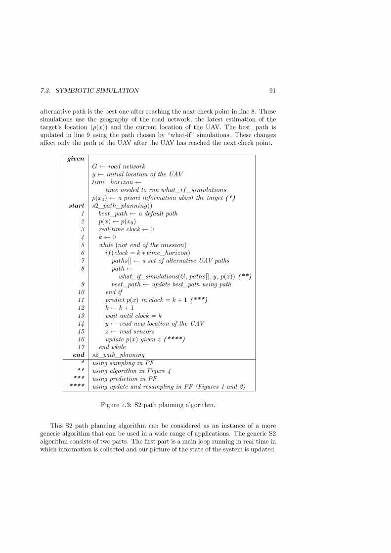
7.3. SYMBIOTIC SIMULATION 91
alternative path is the best one after reaching the next check point in line 8. Thesesimulations use the geography of the road network, the latest estimation of thetarget’s location (p(x)) and the current location of the UAV. The best_path isupdated in line 9 using the path chosen by “what-if” simulations. These changesaffect only the path of the UAV after the UAV has reached the next check point.
givenG← road networky ← initial location of the UAVtime_horizon←
time needed to run what_if_simulationsp(x0)← a priori information about the target (*)
start s2_path_planning()1 best_path← a default path2 p(x)← p(x0)3 real-time clock ← 04 k ← 05 while (not end of the mission)6 if(clock = k ∗ time_horizon)7 paths[]← a set of alternative UAV paths8 path←
what_if_simulations(G, paths[], y, p(x)) (**)9 best_path← update best_path using path
10 end if11 predict p(x) in clock = k + 1 (***)12 k ← k + 113 wait until clock = k14 y ← read new location of the UAV15 z ← read sensors16 update p(x) given z (****)17 end while
end s2_path_planning* using sampling in PF
** using algorithm in Figure 4*** using prediction in PF
**** using update and resampling in PF (Figures 1 and 2)
Figure 7.3: S2 path planning algorithm.
This S2 path planning algorithm can be considered as an instance of a moregeneric algorithm that can be used in a wide range of applications. The generic S2algorithm consists of two parts. The first part is a main loop running in real-time inwhich information is collected and our picture of the state of the system is updated.
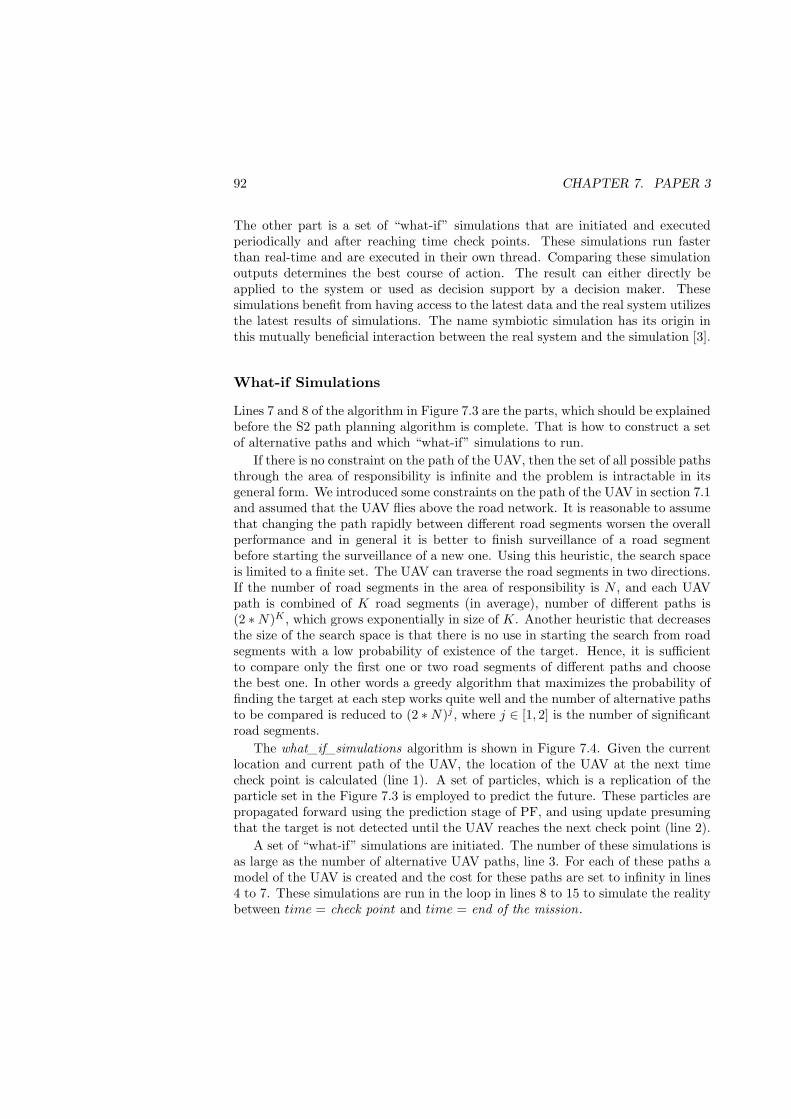
92 CHAPTER 7. PAPER 3
The other part is a set of “what-if” simulations that are initiated and executedperiodically and after reaching time check points. These simulations run fasterthan real-time and are executed in their own thread. Comparing these simulationoutputs determines the best course of action. The result can either directly beapplied to the system or used as decision support by a decision maker. Thesesimulations benefit from having access to the latest data and the real system utilizesthe latest results of simulations. The name symbiotic simulation has its origin inthis mutually beneficial interaction between the real system and the simulation [3].
What-if Simulations
Lines 7 and 8 of the algorithm in Figure 7.3 are the parts, which should be explainedbefore the S2 path planning algorithm is complete. That is how to construct a setof alternative paths and which “what-if” simulations to run.
If there is no constraint on the path of the UAV, then the set of all possible pathsthrough the area of responsibility is infinite and the problem is intractable in itsgeneral form. We introduced some constraints on the path of the UAV in section 7.1and assumed that the UAV flies above the road network. It is reasonable to assumethat changing the path rapidly between different road segments worsen the overallperformance and in general it is better to finish surveillance of a road segmentbefore starting the surveillance of a new one. Using this heuristic, the search spaceis limited to a finite set. The UAV can traverse the road segments in two directions.If the number of road segments in the area of responsibility is N , and each UAVpath is combined of K road segments (in average), number of different paths is(2 ∗N)K , which grows exponentially in size of K. Another heuristic that decreasesthe size of the search space is that there is no use in starting the search from roadsegments with a low probability of existence of the target. Hence, it is sufficientto compare only the first one or two road segments of different paths and choosethe best one. In other words a greedy algorithm that maximizes the probability offinding the target at each step works quite well and the number of alternative pathsto be compared is reduced to (2 ∗N)j , where j ∈ [1, 2] is the number of significantroad segments.
The what_if_simulations algorithm is shown in Figure 7.4. Given the currentlocation and current path of the UAV, the location of the UAV at the next timecheck point is calculated (line 1). A set of particles, which is a replication of theparticle set in the Figure 7.3 is employed to predict the future. These particles arepropagated forward using the prediction stage of PF, and using update presumingthat the target is not detected until the UAV reaches the next check point (line 2).
A set of “what-if” simulations are initiated. The number of these simulations isas large as the number of alternative UAV paths, line 3. For each of these paths amodel of the UAV is created and the cost for these paths are set to infinity in lines4 to 7. These simulations are run in the loop in lines 8 to 15 to simulate the realitybetween time = check point and time = end of the mission.

7.3. SYMBIOTIC SIMULATION 93
givenpath : current path of the UAVpaths[] : a finite set of UAV paths to be comparedy : current location of the UAVp(x) : current information about the target
start what_if_simulations(path, paths[], y, p(x))1 y ← location of the UAV in time_horizon given
current location y and path2 p(x)← future state of the target given p(x) and it
is not detected in time_horizon by UAV3 nr of simulations ← size of paths[]4 for (i = 1 : nr of simulations )5 uavs[i]← a UAV model located at y6 path of uavs[i]← paths[i]7 costs[i]←∞
end for8 for (k = check point : end of the mission )9 predict p(x) using p(xk | xk−1)
10 for (i = 1 : nr of simulations )11 move uavs[i] having paths[i]12 estimate uavs[i] observation using p(zk | xk)13 costs[i]← calculate the cost for paths[i]14 end for15 end for16 min← argmin
i(costs[i])
17 return paths[min]end what_if_simulations
Figure 7.4: “What if simulations” algorithm
At each time step of the simulation using prediction stage, p(xk | xk−1), the newstate of the target is estimated (line 9). Care should be taken that these particlesare not the same particle used in the S2 path planning algorithm, but a replicationof them. The original particles in S2 path planning always reflect our estimationof the target in real-time, but what-if simulations run faster than the real-timeand provide an estimation of the location of the target in future by repeatingthe prediction stage. Note that in the algorithm in Figure 7.4, it is implicitlyassumed that the future stat of the target in different cases is independent of thelocation of the UAV. Loosely formulated, we compare the impact of our differentcourses of action in the same simulated future. This assumption reduces the run-time complexity of the algorithm by assembling all what-if simulations in a singlesimulation running on a single process/thread. However, it may not always be the
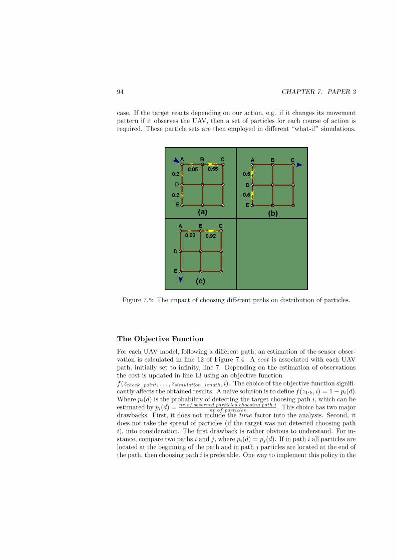
94 CHAPTER 7. PAPER 3
case. If the target reacts depending on our action, e.g. if it changes its movementpattern if it observes the UAV, then a set of particles for each course of action isrequired. These particle sets are then employed in different “what-if” simulations.
Figure 7.5: The impact of choosing different paths on distribution of particles.
The Objective Function
For each UAV model, following a different path, an estimation of the sensor obser-vation is calculated in line 12 of Figure 7.4. A cost is associated with each UAVpath, initially set to infinity, line 7. Depending on the estimation of observationsthe cost is updated in line 13 using an objective functionf(zcheck_point, . . . , zsimulation_length, i). The choice of the objective function signifi-cantly affects the obtained results. A naive solution is to define f(z1:k, i) = 1− pi(d).Where pi(d) is the probability of detecting the target choosing path i, which can beestimated by pi(d) = nr of observed particles choosing path i
nr of particles . This choice has two majordrawbacks. First, it does not include the time factor into the analysis. Second, itdoes not take the spread of particles (if the target was not detected choosing pathi), into consideration. The first drawback is rather obvious to understand. For in-stance, compare two paths i and j, where pi(d) = pj(d). If in path i all particles arelocated at the beginning of the path and in path j particles are located at the end ofthe path, then choosing path i is preferable. One way to implement this policy in the
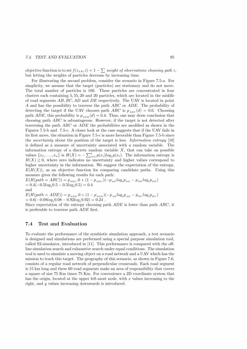
7.4. TEST AND EVALUATION 95
objective function is to set f(z1:k, i) = 1−∑
weight of observations choosing path i ,but letting the weights of particles decrease by increasing time.
For illustrating the second problem, consider the scenario in Figure 7.5-a. Forsimplicity, we assume that the target (particles) are stationary and do not move.The total number of particles is 100. These particles are concentrated in fourclusters each containing 5, 55, 20 and 20 particles, which are located in the middleof road segments AB,BC,AD and DE respectively. The UAV is located in pointA and has the possibility to traverse the path ABC or ADE. The probability ofdetecting the target if the UAV chooses path ABC is p
ABC(d) = 0.6. Choosing
path ADE, this probability is pADE
(d) = 0.4. Thus, one may draw conclusion thatchoosing path ABC is advantageous. However, if the target is not detected aftertraversing the path ABC or ADE the probabilities are modified as shown in theFigures 7.5-b and 7.5-c. A closer look at the case suggests that if the UAV fails inits first move, the situation in Figure 7.5-c is more favorable than Figure 7.5-b sincethe uncertainty about the position of the target is less. Information entropy [10]is defined as a measure of uncertainty associated with a random variable. Theinformation entropy of a discrete random variable X, that can take on possiblevalues {x1, . . . , xn} is H(X) = −
∑ni=1 p(xi)log2p(xi). The information entropy is
H(X) ≥ 0, where zero indicates no uncertainty and higher values correspond tohigher uncertainty in the information. We suggest the expectation of the entropy,E(H(X)), as an objective function for comparing candidate paths. Using thismeasure gives the following results for each path:E(H(path = ABC)) = p
ABC.0 + (1− p
ABC)(−p
ADlog2pAD
− pDE
log2pDE)
= 0.4(−0.5log20.5− 0.5log20.5) = 0.4andE(H(path = ADE)) = p
ADE.0 + (1− p
ADE)(−p
ABlog2pAB
− pBC
log2pBC)
= 0.6(−0.08log20.08− 0.92log20.92) = 0.24 .Since expectation of the entropy choosing path ADE is lower than path ABC, itis preferable to traverse path ADE first.
7.4 Test and Evaluation
To evaluate the performance of the symbiotic simulation approach, a test scenariois designed and simulations are performed using a special purpose simulation tool,called S2-simulator, introduced in [11]. This performance is compared with the off-line simulation search and exhaustive search under equal conditions. The simulationtool is used to simulate a moving object on a road network and a UAV which has themission to track this target. The geography of this scenario, as shown in Figure 7.6,consists of a regular road network of perpendicular crossroads. Each road segmentis 15 km long and these 60 road segments make an area of responsibility that coversa square of size 75 Km times 75 Km. For convenience a 2D coordinate system thathas the origin, located at the upper left-most node, with x values increasing to theright, and y values increasing downwards is introduced.
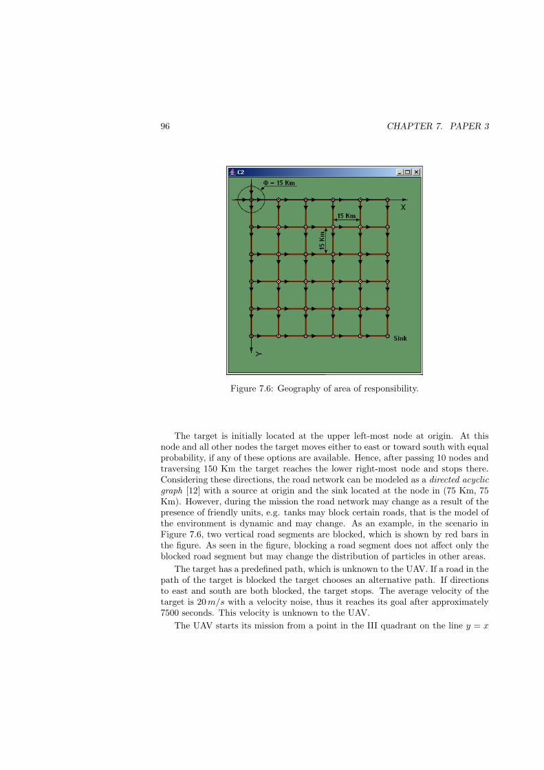
96 CHAPTER 7. PAPER 3
Figure 7.6: Geography of area of responsibility.
The target is initially located at the upper left-most node at origin. At thisnode and all other nodes the target moves either to east or toward south with equalprobability, if any of these options are available. Hence, after passing 10 nodes andtraversing 150 Km the target reaches the lower right-most node and stops there.Considering these directions, the road network can be modeled as a directed acyclicgraph [12] with a source at origin and the sink located at the node in (75 Km, 75Km). However, during the mission the road network may change as a result of thepresence of friendly units, e.g. tanks may block certain roads, that is the model ofthe environment is dynamic and may change. As an example, in the scenario inFigure 7.6, two vertical road segments are blocked, which is shown by red bars inthe figure. As seen in the figure, blocking a road segment does not affect only theblocked road segment but may change the distribution of particles in other areas.
The target has a predefined path, which is unknown to the UAV. If a road in thepath of the target is blocked the target chooses an alternative path. If directionsto east and south are both blocked, the target stops. The average velocity of thetarget is 20 m/s with a velocity noise, thus it reaches its goal after approximately7500 seconds. This velocity is unknown to the UAV.
The UAV starts its mission from a point in the III quadrant on the line y = x
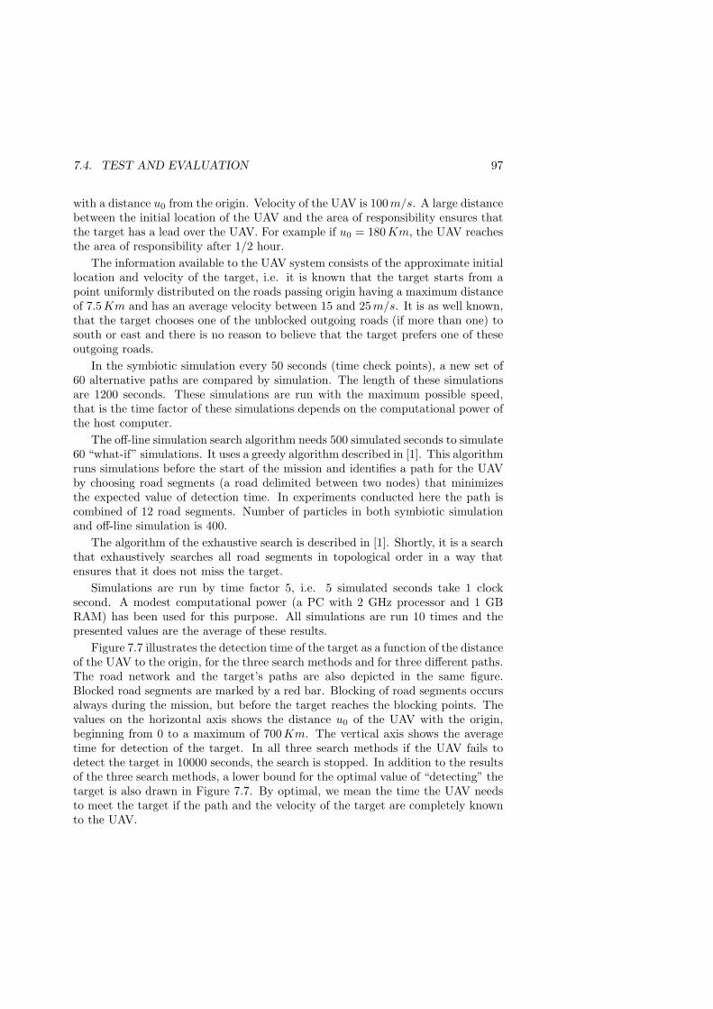
7.4. TEST AND EVALUATION 97
with a distance u0 from the origin. Velocity of the UAV is 100 m/s. A large distancebetween the initial location of the UAV and the area of responsibility ensures thatthe target has a lead over the UAV. For example if u0 = 180Km, the UAV reachesthe area of responsibility after 1/2 hour.
The information available to the UAV system consists of the approximate initiallocation and velocity of the target, i.e. it is known that the target starts from apoint uniformly distributed on the roads passing origin having a maximum distanceof 7.5 Km and has an average velocity between 15 and 25 m/s. It is as well known,that the target chooses one of the unblocked outgoing roads (if more than one) tosouth or east and there is no reason to believe that the target prefers one of theseoutgoing roads.
In the symbiotic simulation every 50 seconds (time check points), a new set of60 alternative paths are compared by simulation. The length of these simulationsare 1200 seconds. These simulations are run with the maximum possible speed,that is the time factor of these simulations depends on the computational power ofthe host computer.
The off-line simulation search algorithm needs 500 simulated seconds to simulate60 “what-if” simulations. It uses a greedy algorithm described in [1]. This algorithmruns simulations before the start of the mission and identifies a path for the UAVby choosing road segments (a road delimited between two nodes) that minimizesthe expected value of detection time. In experiments conducted here the path iscombined of 12 road segments. Number of particles in both symbiotic simulationand off-line simulation is 400.
The algorithm of the exhaustive search is described in [1]. Shortly, it is a searchthat exhaustively searches all road segments in topological order in a way thatensures that it does not miss the target.
Simulations are run by time factor 5, i.e. 5 simulated seconds take 1 clocksecond. A modest computational power (a PC with 2 GHz processor and 1 GBRAM) has been used for this purpose. All simulations are run 10 times and thepresented values are the average of these results.
Figure 7.7 illustrates the detection time of the target as a function of the distanceof the UAV to the origin, for the three search methods and for three different paths.The road network and the target’s paths are also depicted in the same figure.Blocked road segments are marked by a red bar. Blocking of road segments occursalways during the mission, but before the target reaches the blocking points. Thevalues on the horizontal axis shows the distance u0 of the UAV with the origin,beginning from 0 to a maximum of 700 Km. The vertical axis shows the averagetime for detection of the target. In all three search methods if the UAV fails todetect the target in 10000 seconds, the search is stopped. In addition to the resultsof the three search methods, a lower bound for the optimal value of “detecting” thetarget is also drawn in Figure 7.7. By optimal, we mean the time the UAV needsto meet the target if the path and the velocity of the target are completely knownto the UAV.

98 CHAPTER 7. PAPER 3
As expected, regardless of the applied search method, the detection time in-creases by increasing the distance of the UAV to the origin. While exhaustivesearch fails to detect the target before 10000 seconds when u0 exceeds 150 Km, de-tection times remain significantly under 10000 seconds for both off-line simulationand symbiotic simulation search methods for all distances less than 700 Km.
However, the detection time for symbiotic simulation method is generally lessthan detection time for the off-line simulation. In Figures 7.7-a and 7.7-b, detectiontimes for on-line simulation are always less than the corresponding time for off-line simulation. This difference is larger in intervals, where the uncertainty of thelocation of the target is higher. In Figure 7.7-c, even though in some points theoff-line method has a shorter detection time, the overall performance of the on-line method is higher. Moreover, comparing the result of the on-line simulationwith the “optimal” solution in Figures 7.7-a, 7.7-b and 7.7-c, indicates that insome intervals the detection time approaches the optimal value. Optimal value isthe time required to reach the target if the exact information about its path andvelocity is available.
Nevertheless, it should be noted that the statistical superiority of the on-linesimulation method does not guarantee that the detection times for all chosen pathsby the target are always shorter than other methods. The on-line simulation methodonly provides the possibility to adapt the actions with the information model avail-able.
Figure 7.7 suggests that on-line simulation search method in a dynamic en-vironment in most cases shows a higher performance, compared with the off-linesimulation and the exhaustive search method. Only when the UAV’s distance toorigin is less than 100Km, exhaustive search has a shorter detection time thanoff-line simulation method, which can be explained by the fact that the off-linesimulation method has a delay to simulate the entire mission before the start. Forlarger distances the off-line simulation method is superior to the exhaustive searchmethod.
7.5 Conclusions and Future Work
This paper presents an on-line simulation-aided UAV path planning for tracking asingle target on a pre-known road network. These simulations use available a prioriinformation to prioritize searching in areas with higher probability of the existenceof the target. Simulations are performed using a special purpose simulation toolto test this method on a designed scenario. The results of the on-line simulationpath planning is compared with two other path planning methods: an off-linesimulation-aided path planning and an exhaustive search method. The conductedsimulations indicate that the on-line simulation path planning has generally a higherperformance compared with the two other methods.
One natural extension to the suggested symbiotic simulation path planning isto employ this method in more complex scenarios involving more than one target
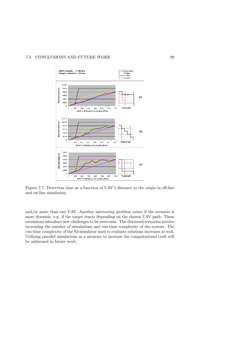
7.5. CONCLUSIONS AND FUTURE WORK 99
Figure 7.7: Detection time as a function of UAV’s distance to the origin in off-lineand on-line simulation.
and/or more than one UAV. Another interesting problem arises if the scenario ismore dynamic, e.g. if the target reacts depending on the chosen UAV path. Theseextensions introduce new challenges to be overcome. The discussed scenarios involveincreasing the number of simulations and run-time complexity of the system. Therun-time complexity of the S2-simulator used to evaluate solutions increases as well.Utilizing parallel simulations as a measure to increase the computational craft willbe addressed in future work.


Bibliography
[1] Farzad Kamrani and Rassul Ayani. Simulation-aided path planning of UAV.In (to appear) Proceedings of the Winter Simulation Conference, Dec 2007.
[2] Eric W. Weisstein. Topological sort, From Mathworld–A Wolfram web resource, 2000. Available viahttp://mathworld.wolfram.com/TopologicalSort.html [accessed March 29,2007].
[3] Richard Fujimoto, Dell Lunceford, Ernest Page, and Adelinde M. Uhrmacher.Summary of the Parallel/Distributed Simulation Working Group. In RichardFujimoto, Dell Lunceford, Ernest Page, and Adelinde M. Uhrmacher, editors,Grand Challenges for Modeling and Simulation, Dagstuhl Report, pages 49–52,August 2002.
[4] Malcolm Yoke Hean Low, Kong Wei Lye, Peter Lendermann, Stephen JohnTurner, Reman Tat Wee Chim, and Surya Hadisaputra Leo. An agent-basedapproach for managing symbiotic simulation of semiconductor assembly andtest operation. In Proceedings of the fourth international joint conference onAutonomous agents and multiagent systems, pages 85–92, 2005.
[5] Wolfgang Koch. On ‘negative’ information in tracking and sensor data fusion:Discussion of selected examples. In Proceedings of the Seventh InternationalConference on Information Fusion, volume I, pages 91–98, Jun 2004.
[6] Arnaud Doucet, Nando de Freitas, and Neil Gordon. Sequential Monte CarloMethods in Practice. Springer Verlag, 2001.
[7] S. Arulampalam, S. Maskell, N. Gordon, and T. Clapp. A tutorial on ParticleFilters for on-line non-linear/non-gaussian bayesian tracking. IEEE Transac-tions on Signal Processing, 50(2):174–188, February 2002.
[8] Simon Ahlberg, Pontus Hörling, Karsten Jöred, Christian Mårtenson, GöranNeider, Johan Schubert, Hedvig Sidenbladh, Pontus Svenson, Per Svensson,Katarina Undén, and Johan Walter. The IFD03 information fusion demon-strator. In Proceedings of the Seventh International Conference on InformationFusion, volume II, pages 936–943, Jun 2004.
101

102 BIBLIOGRAPHY
[9] Branko Ristic, Sanjeev Arulampalam, and Neil Gordon. Beyond the KalmanFilter: Particle Filters for Tracking Applications. Artech House Series Pub-lishers, 2004.
[10] David J. C. Mackay. Information Theory, Inference, and Learning Algorithms.Cambridge University Press, 2005.
[11] Farzad Kamrani, Marianela Garcia Lozano, and Rassul Ayani. Path planningfor UAVs using symbiotic simulation. In Proceedings of the 20th annual Eu-ropean Simulation and Modelling Conference, ESM’2006, pages 215–238, Oct2006.
[12] Eric W. Weisstein. Acyclic digraph, From Mathworld–A Wolfram web resource, 2003. Available viahttp://mathworld.wolfram.com/AcyclicDigraph.html [accessed March 29,2007].