
UNIVERSIDAD COMPLUTENSE DE MADRIDeprints.ucm.es/24558/1/T35146.pdf · mano de Dios, carne de...
145
UNIVERSIDAD COMPLUTENSE DE MADRID FACULTAD DE CIENCIAS FÍSICAS TESIS DOCTORAL Definition and properties of transverse momentum distributions Definición y propiedades de las distribuciones de momento transverso MEMORIA PARA OPTAR AL GRADO DE DOCTOR PRESENTADA POR Miguel García Echevarría Director Ignazio Scimeni Madrid, 2014 © Miguel García Echevarría, 2013
Transcript of UNIVERSIDAD COMPLUTENSE DE MADRIDeprints.ucm.es/24558/1/T35146.pdf · mano de Dios, carne de...
UNIVERSIDAD COMPLUTENSE DE MADRID
FACULTAD DE CIENCIAS FÍSICAS
TESIS DOCTORAL
Definition and properties of transverse momentum distributions
Definición y propiedades de las distribuciones de momento
transverso
MEMORIA PARA OPTAR AL GRADO DE DOCTOR
PRESENTADA POR
Miguel García Echevarría
Director
Ignazio Scimeni
Madrid, 2014
© Miguel García Echevarría, 2013
Definition and Properties of
Transverse Momentum Distributions
by
Miguel García Echevarría
under the supervision of
Dr. Ignazio Scimemi
A dissertation submitted in partial fulfillment of the requirements for the Degree of Doctor of
Philosophy in Physics.
Facultad de Ciencias Físicas
Madrid, December 2013

Acknowledgements
To begin with, I would like to thank my advisor, Ignazio Scimemi, for his guidance and patience over
these last years. His office door was always opened and he accompanied my growth as a scientist, giving me
the liberty to face research tasks alone so I could learn, helping me out when I was stuck and encouraging
me when I needed.
I would also like to thank my collaborator Ahmad Idilbi, my second boss, for fruitful years of research,
full of experiences, hard work, advises and discussions. From the very beginning he trusted me as much as
challenged me, so that I could give the best of me.
During the PhD I shared office with great fellow scientists and better persons, from whom I learned
and with whom I had a lot of fun. They are joined by the rest of the people from Theoretical Physics
Department II at UCM, where this thesis was completed, Theoretical Physics Department I and the faculty
in general, to whom I am also grateful. All of them made this experience much richer.
I thank as well the professors and staff of my department, for their help, kindness and availability when
needed. A special mention deserve Antonio Dobado and José Ramón Peláez, who managed the research
projects that allowed me to go abroad, meet interesting people and grow scientifically and personally. I am
thankful to Prof. Christian Bauer at Lawrence Berkeley National Laboratory, where I spent three months,
and to Prof. Andreas Schäfer at University of Regensburg, where I made a couple of short visits, for their
hospitality and support.
Around ten years ago I started studying Physics at the Basque Country, and I cannot forget about
all my fellow undergrad students. We made a great team along the years, grew together, worked together,
learned from each other and encouraged each other to pursue our dream of becoming good researchers. I
am really grateful to each of them, as well as all the professors we had.
Finally, my most sincere thanks to my family and friends, specially my mother and my aunts, for
their love, encouragement and understanding. They taught me the passion for knowledge, the humility of
ignorance and the value of hard work.

List of publications
The following articles have been produced in the context of this dissertation:
• SCET, Light-Cone Gauge and the T-Wilson Lines.
Miguel G. Echevarria, Ahmad Idilbi and Ignazio Scimemi.
Phys. Rev. D 84 (2011) 011502. [arXiv:1104.0686 [hep-ph]].
• Factorization Theorem for Drell-Yan at Low qT and Transverse Momentum Distributions
On-The-Light-Cone.
Miguel G. Echevarria, Ahmad Idilbi and Ignazio Scimemi.
JHEP 1207 (2012) 002. [arXiv:1111.4996 [hep-ph]].
• Model-Independent Evolution of Transverse Momentum Dependent Distribution Func-
tions (TMDs) at NNLL.
Miguel G. Echevarria, Ahmad Idilbi, Andreas Schäfer and Ignazio Scimemi.
Accepted for publication in Eur. Phys. J. C. [arXiv:1208.1281 [hep-ph]].
• Soft and Collinear Factorization and Transverse Momentum Dependent Parton Distribu-
tion Functions.
Miguel G. Echevarria, Ahmad Idilbi and Ignazio Scimemi.
Phys. Lett. B 726 (2013) 795-801. [arXiv:1211.1947 [hep-ph]].
The author has also contributed to the following conference proceedings:
• Definition and Evolution of Transverse Momentum Distributions.
Miguel G. Echevarria, Ahmad Idilbi and Ignazio Scimemi.
Int.J.Mod.Phys.Conf.Ser. 20 (2012) 92-108.
• Proper definition of transverse momentum dependent distributions.
Miguel G. Echevarria, Ahmad Idilbi and Ignazio Scimemi.
AIP Conf. Proc. 1523 (2012) 174.
• The Evolution of Transverse Momentum Distribution Functions at NNLL.
Miguel G. Echevarria, Ahmad Idilbi, Andreas Schäfer and Ignazio Scimemi.
PoS ConfinementX (2012) 096.

Contents
Acknowledgements i
List of publications iii
Prelude 1
1 Introduction to Soft-Collinear Effective Theory 5
1.1 Motivation . . . . . . . . . . . . . . . . . . . . . . . . . . . . . . . . . . . . . . . . . . . . . . 5
1.2 SCET-I Lagrangian . . . . . . . . . . . . . . . . . . . . . . . . . . . . . . . . . . . . . . . . . . 7
1.2.1 Collinear Quark Lagrangian . . . . . . . . . . . . . . . . . . . . . . . . . . . . . . . . . 7
1.2.2 Wilson Lines . . . . . . . . . . . . . . . . . . . . . . . . . . . . . . . . . . . . . . . . . 10
1.2.3 Collinear Gluon Lagrangian . . . . . . . . . . . . . . . . . . . . . . . . . . . . . . . . . 12
1.2.4 Ultrasoft Lagrangian . . . . . . . . . . . . . . . . . . . . . . . . . . . . . . . . . . . . . 13
1.2.5 Usoft Interactions with Collinear Quarks and Gluons . . . . . . . . . . . . . . . . . . . 13
1.3 Symmetries in SCET-I . . . . . . . . . . . . . . . . . . . . . . . . . . . . . . . . . . . . . . . . 15
1.3.1 Gauge Symmetry in SCET . . . . . . . . . . . . . . . . . . . . . . . . . . . . . . . . . 15
1.3.2 Reparameterization Invariance SCET . . . . . . . . . . . . . . . . . . . . . . . . . . . 16
1.4 SCET-II . . . . . . . . . . . . . . . . . . . . . . . . . . . . . . . . . . . . . . . . . . . . . . . . 17
1.5 Factorization of the Quark Form Factor . . . . . . . . . . . . . . . . . . . . . . . . . . . . . . 17
1.5.1 DIS Kinematics . . . . . . . . . . . . . . . . . . . . . . . . . . . . . . . . . . . . . . . . 18
1.5.2 DY Kinematics . . . . . . . . . . . . . . . . . . . . . . . . . . . . . . . . . . . . . . . . 23
2 Soft-Collinear Effective Theory in Light-Cone Gauge 29
2.1 Introduction . . . . . . . . . . . . . . . . . . . . . . . . . . . . . . . . . . . . . . . . . . . . . . 29
2.2 The T-Wilson lines . . . . . . . . . . . . . . . . . . . . . . . . . . . . . . . . . . . . . . . . . . 30
2.2.1 SCET-I Lagrangian in LCG . . . . . . . . . . . . . . . . . . . . . . . . . . . . . . . . . 32
2.2.2 SCET-II Lagrangian in LCG . . . . . . . . . . . . . . . . . . . . . . . . . . . . . . . . 32
2.3 Applications . . . . . . . . . . . . . . . . . . . . . . . . . . . . . . . . . . . . . . . . . . . . . . 33
2.4 Factorization of the Quark Form Factor in LCG . . . . . . . . . . . . . . . . . . . . . . . . . . 34
2.4.1 Quark Form Factor in QCD in LCG . . . . . . . . . . . . . . . . . . . . . . . . . . . . 36
2.4.2 Quark Form Factor in SCET in LCG . . . . . . . . . . . . . . . . . . . . . . . . . . . . 39
3 Drell-Yan TMD Factorization 41
3.1 Introduction . . . . . . . . . . . . . . . . . . . . . . . . . . . . . . . . . . . . . . . . . . . . . . 41
3.2 Factorization of Drell-Yan at Small qT . . . . . . . . . . . . . . . . . . . . . . . . . . . . . . . 44
3.3 Collinear and Soft Matrix Elements at O(αs) . . . . . . . . . . . . . . . . . . . . . . . . . . . 46
3.3.1 Collinear Matrix Element Jn(n) . . . . . . . . . . . . . . . . . . . . . . . . . . . . . . . 47
3.3.2 Soft Function S . . . . . . . . . . . . . . . . . . . . . . . . . . . . . . . . . . . . . . . . 50
3.4 Equivalence of Soft and Zero-Bin Subtractions . . . . . . . . . . . . . . . . . . . . . . . . . . 51
3.5 Extraction of the Hard Coefficient H at O(αs) . . . . . . . . . . . . . . . . . . . . . . . . . . 52
3.6 Preliminary Definition of the TMDPDF . . . . . . . . . . . . . . . . . . . . . . . . . . . . . . 54
3.6.1 Anomalous Dimension in Dimensional Regularization . . . . . . . . . . . . . . . . . . 55
3.7 Refactorization: from TMDPDF to PDF . . . . . . . . . . . . . . . . . . . . . . . . . . . . . . 56
3.7.1 Q2-Dependence and Resummation . . . . . . . . . . . . . . . . . . . . . . . . . . . . . 59
3.8 The Proper Definition of TMDPDF . . . . . . . . . . . . . . . . . . . . . . . . . . . . . . . . 63
3.8.1 Divergences in the Soft Function . . . . . . . . . . . . . . . . . . . . . . . . . . . . . . 66
3.8.2 Splitting the Soft Function . . . . . . . . . . . . . . . . . . . . . . . . . . . . . . . . . 67
3.9 Equivalence of EIS and JCC Definitions . . . . . . . . . . . . . . . . . . . . . . . . . . . . . . 71
3.10 TMDPDF in Light-Cone Gauge . . . . . . . . . . . . . . . . . . . . . . . . . . . . . . . . . . . 74
vi Contents
4 Evolution of TMDPDFs 77
4.1 Introduction . . . . . . . . . . . . . . . . . . . . . . . . . . . . . . . . . . . . . . . . . . . . . . 77
4.2 Definition of Quark-TMDPDF . . . . . . . . . . . . . . . . . . . . . . . . . . . . . . . . . . . 78
4.3 Evolution Kernel . . . . . . . . . . . . . . . . . . . . . . . . . . . . . . . . . . . . . . . . . . . 79
4.3.1 Derivation of DR . . . . . . . . . . . . . . . . . . . . . . . . . . . . . . . . . . . . . . . 80
4.3.2 Range of Validity of DR and the Landau Pole . . . . . . . . . . . . . . . . . . . . . . . 82
4.3.3 Applicability of the Evolution Kernel . . . . . . . . . . . . . . . . . . . . . . . . . . . . 83
4.4 An Alternative Extraction of DR . . . . . . . . . . . . . . . . . . . . . . . . . . . . . . . . . . 85
4.5 Comparison with CSS Approach . . . . . . . . . . . . . . . . . . . . . . . . . . . . . . . . . . 86
5 Semi-Inclusive Deep-Inelastic Scattering TMD Factorization 91
5.1 Factorization of SIDIS at Small qT . . . . . . . . . . . . . . . . . . . . . . . . . . . . . . . . . 91
5.2 Universality of the TMDPDF . . . . . . . . . . . . . . . . . . . . . . . . . . . . . . . . . . . . 93
5.3 TMDFF at O(αs) . . . . . . . . . . . . . . . . . . . . . . . . . . . . . . . . . . . . . . . . . . 97
5.4 Extraction of the Hard Coefficient . . . . . . . . . . . . . . . . . . . . . . . . . . . . . . . . . 101
5.5 Refactorization: from TMDFF to FF . . . . . . . . . . . . . . . . . . . . . . . . . . . . . . . . 102
5.6 Evolution of TMDFFs . . . . . . . . . . . . . . . . . . . . . . . . . . . . . . . . . . . . . . . . 105
Conclusions 107
A TMDPDF onto PDF Matching for SIDIS 109
B CSS Approach to the Evolution of TMDs 113
C Evolution of the Hard Matching Coefficient 115
D Derivation of DR at NNNLL 117
Summary 119
Resumen 125
Bibliography 131

A mi padre y mi abuela...
Himno a la Materia
Bendita seas tú, áspera Materia, gleba estril, dura roca, tú que no cedes más que a la violencia y nos obligas
a trabajar si queremos comer.
Bendita seas, peligrosa Materia, mar violenta, indomable pasión, tú que nos devoras si no te encadenamos.
Benditas seas, poderosa Materia, evolución irresistible, realidad siempre naciente, tú que haces estallar en
cada momento nuestros esquemas y nos obligas a buscar cada vez más lejos la verdad.
Bendita seas, universal Materia, duración sin límites, éter sin orillas, triple abismo de las estrellas, de los
átomos y de las generaciones, tú que desbordas y disuelves nuestras estrechas medidas y nos revelas las
dimensiones de Dios.
Bendita seas, Materia mortal, tú que, disociándote un día en nosotros, nos introducirás, por fuerza, en el
corazón mismo de lo que es. Sin ti, Materia, sin tus ataques, sin tus arranques, viviríamos inertes,
estancados, pueriles, ignorantes de nosotros mismo y de Dios. Tú que castigas y que curas, tú que resistes
y que cedes, tú que trastruecas y que construyes, tú que encadenas y que liberas, savia de nuestras almas,
mano de Dios, carne de Cristo, Materia, yo te bendigo.
Yo te bendigo, Materia, y te saludo, no como te describen, reducida o desfigurada, los pontífices de la
ciencia y los predicadores de la virtud, un amasijo, dicen de fuerzas brutales o de bajos apetitos, sino como
te me apareces hoy, en tu totalidad y tu verdad.
Te saludo, inagotable capacidad de ser y de transformación en donde germina y crece la sustancia elegida.
Te saludo, potencia universal de acercamiento y de unión mediante la cual se entrelaza la muchedumbre de
las mónadas y en la que todas convergen en el camino del Espíritu.
Te saludo, fuente armoniosa de las almas, cristal límpido de donde ha surgido la nueva Jerusalén.
Te saludo, medio divino, cargado de poder creador, océano agitado por el Espíritu, arcilla amasada y
animada por el Verbo encarnado.
Creyendo obedecer a tu irresistible llamada, los hombres se precipitan con frecuencia por amor hacia ti en
el abismo exterior de los goces egośitas.
Les engaña un reflejo o un eco.
Lo veo ahora.
Para llegar a ti, Materia, es necesario que, partiendo de un contacto universal con todo lo que se mueve
aquí abajo, sintamos poco a poco cójo se desvanecen entre nuestras manos las formas particulares de todo lo
que cae a nuestro alcance, hasta que nos encontremos frente a la única esencia de todas las consistencias y
de todas las uniones.
Si queremos conservarte, hemos de sublimarte en el dolor después de haberte estrechado voluptuosamente
entre nuestros brazos.
Tú, Materia, reinas en las serenas alturas en las que los santos se imaginan haberte dejado a un lado;
carne tan transparente y tan móvil que ya no te distinguimos de un espíritu.
¡Arrebátanos, oh, Materia, allá arriba, mediante el esfuerzo, la separación y la muerte!; arrebátame allí en
donde al fin sea posible abrazar castamente al Universo.
Pierre Teilhard de Chardin, sj.

PreludeThere are four known fundamental interactions in nature: gravitational, electromagnetic, weak and
strong interactions. The former one is well described by the General Relativity theory. The other three are
combined into the Standard Model (SM), a relativistic quantum field theory built with the guidance of gauge
invariance and renormalizability. It is given in terms of a Lagrangian of quantized fields that describe the
elementary degrees of freedom, quarks and leptons, and the carriers of the interactions, the bosons. The SM
is divided in two sectors: the electroweak sector, which unifies the electromagnetic and weak interactions,
and the strong sector, described by Quantum Chromodynamics (QCD).
Understanding QCD has been pursued over for almost four decades from different perspectives: pertur-
bative QCD, lattice QCD, effective field theories (chiral perturbation theory, heavy-quark effective theory,
soft-collinear effective theory, etc), and other frameworks as well. Despite many efforts, the question of how
the observed properties of hadrons are generated by the dynamics of their constituents, namely quarks and
gluons, is yet to be resolved. A research venue that would be of much help, and which is being actively pur-
sued both theoretically and experimentally, is to try to explore the three-dimensional structure of nucleons,
both in momentum and configuration space. The role of quarks and gluons in generating the nucleon’s spin
or the partonic angular momentum is being investigated in experimental facilities such as JLab and DESY
and by HERMES, COMPASS or Belle collaborations, among others. The LHC, the most powerful hadron
collider we have nowadays, can also be of very much help in understanding the role of gluons inside the
protons. As mentioned before the ultimate goal is to try to understand how the dynamics of QCD generates
the observed features of hadrons in general and of nucleons in particular.
Among the different physical observables we can deal with, the ones with non-vanishing (or un-
integrated) transverse-momentum dependence are specially important at hadron colliders, and can be very
useful to understand the inner structure of hadrons. Moreover, those observables are relevant for the Higgs
boson searches and also for proper interpretation of signals of physics “beyond the Standard Model”. The
interest in such observables goes back to the first decade immediately after establishing QCD as the funda-
mental theory of strong interactions [1–5]. Recently, however, there has been a much renewed interest in
qT -differential cross sections where hadrons are involved either in the initial states or in the final ones or in
both (see e.g. [6–13]). The main issues of interest range from obtaining an appropriate factorization theorem
for a given process and resumming large logarithmic corrections to performing phenomenological analyses
and predictions.
In order to study the spin and momentum distributions of partons inside the nucleons, it has been
realized that one needs to identify an “irreducible” number of functions (or hadronic matrix elements). In
the collinear limit there are (at leading twist) three parton distribution functions (PDFs), depending on the
polarization of the partons: the momentum distribution [4, 5], the helicity distribution and the transversity
distribution [14]. When the intrinsic partons’ transverse momentum is also considered then one obtains, at
leading twist, eight transverse momentum dependent PDFs (TMDPDFs) 1 that characterize the nucleon’s
internal structure [15,16]. To be of any use, those matrix elements have to be properly defined at the operator
level (in terms of QCD degrees of freedom) and then their properties (such as evolution or universality) should
be carefully examined. Among that group of functions, the unpolarized TMDPDF has a special role. It
has no spin dependence, and thus it is considered as a “simple” generalization of the standard (integrated)
Feynman PDF. However since the introduction of this quantity by Collins and Soper thirty years ago and
despite many efforts [4–6, 10, 17–20], there has not been any agreed-upon definition of it. This fact clearly
has its bearings over the other, and more complicated, hadronic matrix elements as well, and it affects the
whole field of spin physics.
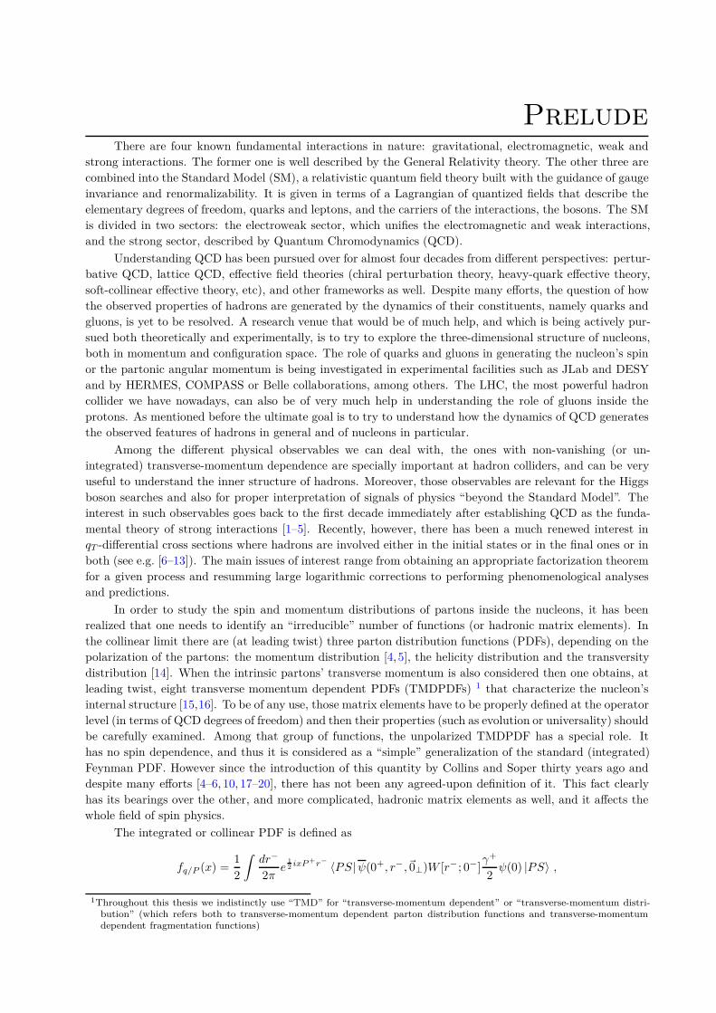
The integrated or collinear PDF is defined as
fq/P (x) =1
2
∫
dr−
2πe
12
ixP +r− 〈PS|ψ(0+, r−,~0⊥)W [r−; 0−]γ+
2ψ(0) |PS〉 ,
1Throughout this thesis we indistinctly use “TMD” for “transverse-momentum dependent” or “transverse-momentum distri-bution” (which refers both to transverse-momentum dependent parton distribution functions and transverse-momentumdependent fragmentation functions)
2 Prelude
where the gauge link W [r−; 0−] connects the two points along the light-cone direction and preserves gauge
invariance (in chapters 1 and 2 it will be more clear the particular form of gauge links). From a probabilistic
point of view, this correlation function gives the number of partons (quarks) inside the nucleon that carry
a fraction x of the collinear momentum P+ of the parent nucleon. This matrix element is a fundamental
block of many factorization theorems. For instance, it appears in the factorization of the structure functions
of DIS [21]. The factorization theorems express a given observable in terms of perturbatively calculable
coefficients and non-perturbative hadronic matrix elements. The formers contain the information of short-
distance physics and do not contain any divergence. The hadronic matrix elements characterize the long-
distance physics of QCD and do have divergences when are calculated perturbatively.
Deriving a factorization theorem for a given hard process is in general a complicated task, and even
more harder it is to prove that it holds to all orders in perturbation theory. As already mentioned, a factor-
ization theorem is the mathematical statement that we can separate the perturbative and non-perturbative
contributions for a given observable, say a cross-section. And in order to be able to formulate it, one needs
to identify first which are the relevant scales and modes that contribute to a given process, and then assign
different matrix elements to them. Moreover, it is easy to imagine that one will find large logarithms of the
ratios of the scales in the perturbative calculations, and thus resummation will play a crucial role in order
to get any sensible results from the established factorization theorems.
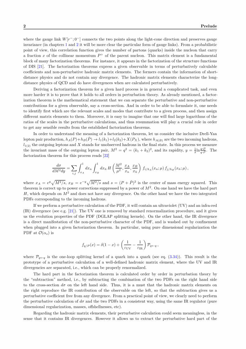
In order to understand the meaning of a factorization theorem, let us consider the inclusive Drell-Yan
lepton pair production, hA(P )+hB(P ) → l1(k1)+l2(k2)+X(PX), where hA(B) are the two incoming hadrons,
l1(2) the outgoing leptons and X stands for unobserved hadrons in the final state. In this process we measure
the invariant mass of the outgoing lepton pair, M2 = q2 = (k1 + k2)2, and its rapidity, y = 12 ln q·P
q·P . The
factorization theorem for this process reads [22]
dσ
dM2dy=∑
i,j
∫ 1
xA
dxn
∫ 1
xB
dxn H
(
M2
µ2,xA
xn,xB
xn
)
fi/hA(xn;µ) fj/hB
(xn;µ) ,
where xA = ey√
M2/s, xB = e−y√
M2/s and s = (P + P )2 is the center of mass energy squared. This
theorem is correct up to power corrections suppressed by a power of M2. On one hand we have the hard part
H , which depends on M2 and does not have any divergence. On the other hand we have the two integrated
PDFs corresponding to the incoming hadrons.
If we perform a perturbative calculation of the PDF, it will contain an ultraviolet (UV) and an infra-red
(IR) divergence (see e.g. [21]). The UV one is removed by standard renormalization procedure, and it gives
us the evolution properties of the PDF (DGLAP splitting kernels). On the other hand, the IR divergence
is a direct manifestation of the non-perturbative character of the PDF, and is washed out by confinement
when plugged into a given factorization theorem. In particular, using pure dimensional regularization the
PDF at O(αs) is
fq/P (x) = δ(1 − x) +
(
1
εUV− 1
εIR
)
Pq←q ,
where Pq←q is the one-loop splitting kernel of a quark into a quark (see eq. (3.34)). This result is the
prototype of a perturbative calculation of a well-defined hadronic matrix element, where the UV and IR
divergencies are separated, i.e., which can be properly renormalized.
The hard part in the factorization theorem is calculated order by order in perturbation theory by
the “subtraction” method, i.e., by subtracting the combination of the two PDFs on the right hand side
to the cross-section dσ on the left hand side. Thus, it is a must that the hadronic matrix elements on
the right reproduce the IR contribution of the observable on the left, so that the subtraction gives us a
perturbative coefficient free from any divergence. From a practical point of view, we clearly need to perform
the perturbative calculation of dσ and the two PDFs in a consistent way, using the same IR regulator (pure
dimensional regularization, masses, offshellnesses, etc).
Regarding the hadronic matrix elements, their perturbative calculation could seem meaningless, in the
sense that it contains IR divergences. However it allows us to extract the perturbative hard part of the
Prelude 3
factorization theorem by the subtraction method. The IR divergences have a clear non-perturbative origin
and are washed out by confinement. In a phenomenological application of the factorization theorem, the
PDFs (and any hadronic matrix element in general) are replaced by numerical functions extracted from the
experiment. Thus, the predictive power of pQCD lies on the universality of the relevant hadronic matrix
elements, which can be extracted from one hard reaction and used to make predictions for another reaction.
With the introduction of Soft-Collinear effective theory (SCET) [23–34] the derivation of factorization
theorems and the resummation of large logarithms has been largely simplified. From the effective theory point
of view one can understand a factorization theorem as a multistep matching procedure. Once the relevant
scales are identified, one needs to perform at each scale a matching between two effective theories, which have
to share the same IR physics. From each matching one will get a perturbative (Wilson) coefficient. At the
end, one will end up with different perturbative coefficients and non-perturbative hadronic matrix elements.
The resummation of large logarithms is done by running the coefficients and/or the matrix elements between
the relevant scales, using the Renormalization Group (RG) equations.
The success of SCET, though, is based on the fact that the relevant modes that reproduce the IR
physics of full QCD are collinear and soft. This is not true in general, and has to be proven (or at least
shown perturbatively and justified to all orders in perturbation theory) for any given process. It lies outside
of the scope of this thesis to analyze the issue related to the appearance of other modes, such as Glauber
modes, and the breakdown of SCET (see e.g. [59]). For the processes we deal with, it is generally believed
that collinear and soft modes do reproduce the IR of QCD, and thus the use of SCET is justified [20,21,35].
Moreover, we have checked this fact explicitly by performing O(αs) calculations.
Focusing back our attention to the transverse momentum of partons, we could think of generalizing
the factorization theorem given previously to the case where we not only measure the invariant mass of the
lepton pair, but also its transverse momentum. In this case, we could schematically write
dσ
dM2dq2⊥dy
=∑
i,j
∫ 1
xA
dxn
∫ 1
xB
dxn
∫
d2kn⊥d2kn⊥δ
(2)(q⊥ − kn⊥ − kn⊥)
×H
(
M2
µ2,xA
xn,xB
xn
)
Fi/hA(xn, kn⊥;µ)Fj/hB
(xn, kn⊥;µ) ,
where the transverse-momentum dependent PDFs (TMDPDFs) would be the generalization of the collinear
PDFs,
Fq/P (x, k⊥) =1
2
∫
dr−d2r⊥(2π)3
e12
ixP +r−−i~k⊥·~r⊥
× 〈PS|ψ(0+, r−, ~r⊥)W [r−; 0−]W [~r⊥;~0⊥]γ+
2ψ(0) |PS〉 .
Notice that we have added a gauge link to connect the points also in the transverse direction. However, if we
perform a perturbative calculation of this quantity we will get rapidity divergences (RDs) and mixed UV/IR
divergences. Thus, this matrix element cannot be renormalized by any means, and it cannot be considered
as a valid hadronic matrix element.
In this thesis, by considering a process which is sensitive to the transverse-momentum of partons inside
the hadrons, and using the effective field theory machinery, we provide a proper definition of TMD hadronic
matrix elements. From their definition and based on the relevant factorization theorem, we obtain their
properties, mainly their evolution, which is of much importance for phenomenological applications and the
whole topic of spin-physics. Thus, three decades after the introduction of the collinear PDF, we complete
the puzzle by providing a proper theoretical definition of the functions that encode the 3-dimensional inner
structure of hadrons: TMDs.
4 Prelude
Outline of the ThesisThe goal of this thesis is to provide a proper definition for TMDs and analyze their properties, mainly
their evolution. By “proper” it is meant basically that these hadronic matrix elements, as measurable
physical quantities, should be free from any rapidity and mixed UV/IR divergences. In order to achieve this
goal we focus on the most simple TMD: the unpolarized TMDPDF.
To start with, in chapter 1 we introduce the effective theory we have used to deal with TMDs: soft-
collinear effective theory. Instead of taking the more standard point of view of perturbative QCD (pQCD), we
choose to benefit from the machinery of SCET, which has proven to be very useful in deriving factorization
theorem, performing perturbative calculations and resumming large logarithms for different observables.
Notice that the use of SCET does not reduce the scope of validity of the results in this thesis. On the
contrary, it is just a different “language” to deal with QCD in the high-energy limit, where the relevant
modes that reproduce the long-distance physics of QCD are soft and collinear. In some sense, we could
say that SCET is the “modern” tool to understand this scenario, which has the advantages of a solid and
well-structured effective field theory.
One of the features of TMDs is that they involve correlators that have a separation not only in the
light-cone direction, but also in the transverse, posing a challenge for their gauge invariance. For this kind
of matrix elements we need collinear and transverse gauge links as well, that preserve the gauge invariance
between, for instance, Feynman and light-cone gauges. As will be explained, the existing formulation of SCET
was done only for covariant gauges, thus failing in singular gauges and not being suitable for obtaining a
gauge invariant definition of TMDs in particular, and for any correlator with separation in the transverse
direction in general. In chapter 2 we explain the origin of a new transverse gauge links (Wilson lines) within
the formalism of SCET, thus extending this theory in order to properly define this kind of correlators.
Once we have modified SCET to make it suitable to deal with processes where the transverse momentum
plays an important role, we focus our attention in chapter 3 on the qT -spectrum of Drell-Yan heavy-lepton
pair production. In this process, the relevant TMDs are the unpolarized TMDPDFs corresponding to the
colliding hadrons, and represent the most simple TMD we can study. By deriving a factorization theorem
for this process using SCET, we are able to identify the problematic issues around TMDs and obtain a
well-defined TMDPDF, free from rapidity and mixed UV/IR divergences. This fact is shown explicitly by
performing a one-loop calculation. Moreover, we analyze the collinear expansion of the TMDPDF in terms of
the standard Feynman PDF. In other words, and from the effective theory point of view, by doing an operator
product expansion of the TMDPDF onto the collinear PDF we integrate out the transverse-momentum in
terms of a Wilson coefficient. And finally, in chapter 3 we also obtain the ingredients necessary to evolve
the TMDPDF at NNLL accuracy.
In chapter 4 we focus on the evolution of TMDPDFs. By combining the anomalous dimension and
the Q2-exponentiation of the TMDPDF obtained in the previous chapter, we build an evolution kernel valid
for all leading-twist TMDPDFs, as the unpolarized distribution, Sivers function or Boer-Mulders function.
This evolution kernel allows us to evolve the TMDPDFs at the highest possible accuracy, NNLL, given the
available perturbative ingredients we have at our disposal nowadays. Under certain kinematical conditions,
we show that the evolution of TMDs can be performed in a perturbative way, without needing to introduce
any ad-hoc model. This presents a major step towards the phenomenological study of TMDPDFs, since
the model-dependence is restricted to the low-energy TMDPDFs themselves, and not their evolution. We
compare our method with the more standard Collins-Soper-Sterman one, finding a complete agreement in
the perturbative region.
Finally, in chapter 5 we consider semi-inclusive deep inelastic scattering, obtain its factorization theorem
by using SCET machinery and properly define the TMDFF, following the previous steps on Drell-Yan. We
calculate the TMDFF at O(αs), its matching coefficient onto the collinear FF and discuss its evolution
properties. It turns out that the evolution kernel for TMDFFs is the same as for TMDPDFs, and thus all
the results in chapter 4 can be straightforwardly applied to the evolution TMDFFs.
1Introduction to Soft-Collinear
Effective TheorySoft-Collinear Effective Theory (SCET) is an effective field theory that describes the interactions be-
tween soft and collinear particles. It was first devised to study B-meson decays, however it has proven to be
very useful in describing other processes, such as jet physics, inclusive/exclusive hard reactions, event shapes,
charmonium production, etc. The machinery of factorization and resummation, widely used in perturbative
QCD (pQCD), is greatly simplified from the effective field theory point of view, and in particular, by using
SCET when appropriate.
1.1 Motivation
In processes where the relevant particles are light and energetic, i.e., some component of their mo-
mentum pµ is large while p2 ≈ 0, the separation of short-distance (perturbative) and long-distance (non-
perturbative) effects is tricky. For instance, jet physics or B meson decays are examples of processes driven
by energetic light particles. In fact, SCET was devised to handle the latter, and although nowadays it is
more used for jet physics and other hard processes, we illustrate the kinematics of the theory by considering
a couple of processes involving B mesons.
Let us start by considering the decay B → Xsγ. If we choose the reference frame where the meson is
at rest and the +z direction for the jet Xs, then the momenta of the particles are
pµX = (MB − Eγ , 0, 0, Eγ) ,
pµγ = (Eγ , 0, 0,−Eγ) . (1.1)
Experimentally one needs to impose some cuts to detect the energy of the photon. If we consider the end-
point region where Eγ ≈ MB/2, then MB − 2Eγ = O(ΛQCD). This gives us a large energy EX ≈ MB/2 and
a small invariant mass M2X = MB(MB − 2Eγ) = O(MBΛQCD) for the jet.
If we consider now the process B → ππ, then the momenta of the two pions in the rest frame of the
meson are
pµ = (Eπ , 0, 0,√
E2π −m2
π) ,
pµ = (Eπ , 0, 0,−√
E2π −m2
π) , (1.2)
with Eπ = MB/2 and the two pions onshell: p2 = p2 = m2π.
In these two processes we have different scales corresponding not only to the masses of the particles,
but also to their momenta. In the B → Xsγ process we have MB ∼ Eγ >> M2X ∼ MBΛQCD >> ΛQCD, and
for B → ππ, MB ∼ Eπ >> mπ ∼ ΛQCD. The goal of SCET is to systematically factorize at the Lagrangian
level the relevant kinematical modes. This was done in [23–34].
The expansion parameter that is used in SCET is either η ∼ ΛQCD/Q (SCET-II) either λ ∼√
ΛQCD/Q
(SCET-I), where Q is the typical large scale of the process being considered, usually the energy of collinear
particles. Since we are dealing with particles that move in light-cone directions, it is useful to decompose
the 4-vectors by using the so-called light-cone coordinates. Let us then take two light-like vectors, n and n,
6 1. Introduction to Soft-Collinear Effective Theory
with n2 = n2 = 0 and n · n = 2. If we choose our reference frame in such a way that collinear particles are
along the z axis, then nµ = (1, 0, 0, 1) and nµ = (1, 0, 0,−1). Any vector pµ can be decomposed as
pµ = n·pnµ
2+ n·p n
µ
2+ pµ⊥
≡ p+nµ
2+ p−
nµ
2+ pµ⊥ . (1.3)
The product of two vectors will be
a·b =1
2a+b− +
1
2a−b+ + a⊥·b⊥
=1
2a+b− +
1
2a−b+ − ~a⊥~b⊥ (1.4)
Let us turn back our attention to the two processes we were considering, which will help us identify
the relevant modes we need to build SCET-I and SCET-II. In the B → Xsγ process the relevant momenta
can be decomposed as
pµX = MB
nµ
2+ (MB − 2Eγ)
nµ
2,
pµγ = 2Eγ
nµ
2. (1.5)
The final jet Xs has n·PX = MB and n·PX = MB − 2Eγ ∼ ΛQCD. For B → ππ, on the other hand, we will
have
pµ =MB
2
(
1 +
√
1 − 4m2π
M2B
)
nµ
2+MB
2
(
1 −√
1 − 4m2π
M2B
)
nµ
2,
pµ =MB
2
(
1 −√
1 − 4m2π
M2B
)
nµ
2+MB
2
(
1 +
√
1 − 4m2π
M2B
)
nµ
2, (1.6)
with n·p = n·p ≈ MB and n·p = n·p ≈ m2π/MB ∼ Λ2
QCD/MB. Thus, identifying MB as the large scale
and calling it Q, and using the light-cone coordinates, the relevant modes for B → Xsγ process that can be
derived from eq. (1.5) are
kn ∼ Q(1, λ2, λ) ,
kus ∼ Q(λ2, λ2, λ2) , (1.7)
with λ =√
ΛQCD/Q, which will be described by SCET-I. We have allowed the collinear modes to have a
small transverse component, and also considered the contribution of homogeneous soft modes that scale as
ΛQCD (called “ultrasoft” in the context of SCET-I). On the other hand, the relevant modes for B → ππ that
can be derived from eq. (1.6) are
kn ∼ Q(1, η2, η) ,
ks ∼ Q(η, η, η) , (1.8)
with η = ΛQCD/Q, being SCET-II the proper theory. Notice that the invariant mass of collinear and
soft particles is the same, Q2η2 ∼ Λ2QCD, thus their relative rapidity is the only way to distinguish them.
Furthermore, it is also worth noticing that soft and ultrasoft modes are the same (η ∼ λ2), being the
collinears different in SCET-I and SCET-II.
In the following sections we build the SCET Lagrangians for collinear and (u)soft particles, starting
from the full QCD Lagrangian and considering the proper kinematical regimes. Whenever we write the
scaling of any momentum and do not specify the scale, it should be understood implicitly. For example, if
we write that p ∼ (1, λ2, λ), then we mean p ∼ Q(1, λ2, λ), where λ and Q are related to the relevant scales
1.2. SCET-I Lagrangian 7
in the considered process.
1.2 SCET-I Lagrangian
To find the effective theory Lagrangian we will start from full QCD Lagrangian, which contains all
kinds of modes, and express it in terms of collinear and ultrasoft degrees of freedom. Applying the proper
power counting we will obtain the leading order terms,
L(0) = L(0)nq + L(0)
ng + L(0)us , (1.9)
where L(0)nq(ng) corresponds to the n-collinear quark (gluon) Lagrangian and L(0)
us to the ultrasoft Lagrangian.
Below we usually omit the scale when referring to power counting of fields or momenta. The proper
dimension is recovered by introducing the correct power of the relevant high scale. Thus, for example, the
scaling of a collinear momentum will be written as p ∼ (1, λ2 λ), which refers to p ∼ Q(1, λ2, λ).
1.2.1 Collinear Quark Lagrangian
Let us start from the full QCD Lagrangian for massless quarks,
L = ψ iD/ψ , (1.10)
where Dµ = ∂µ + igtaAaµ. We split the field ψ of a fermion moving in the n direction in two parts, one with
the two large components (ξn) and the other one with the small components (ηn), which can be obtained by
using the projectors,
ψ =n/n/
4ψ +
n/n/
4ψ = ξn + ηn . (1.11)
These fields satisfy
n/n/
4ξn = ξn , n/ξn = 0 ,
n/n/
4ηn = ηn , n/ηn = 0 . (1.12)
In terms of these fields, and expanding the covariant derivative as well, the Lagrangian in eq. (1.10) can be
written as
L = ξnn/
2
(
in·D)
ξn + ηnn/
2
(
in·D)
ηn + ξn
(
iD/⊥
)
ηn + ηn
(
iD/⊥
)
ξn . (1.13)
In order to get this result, notice that
ξniD/⊥ξn = ξniD/⊥n/n/
4ξn = ξn
n/n/
4iD/⊥ξn = 0 , (1.14)
and similarly ηniD/⊥ηn = 0. In the collinear limit, the components ηn are subleading, and thus can be
eliminated from the Lagrangian by using their equation of motion,
δLδηn
= 0 −→ ηn =1
in·DiD/⊥n/
2ξn . (1.15)
8 1. Introduction to Soft-Collinear Effective Theory
Using this result, the Lagrangian in eq.(1.13) is simplified as
L = ξn
(
in·D + iD/⊥1
in·DiD/⊥)
n/
2ξn . (1.16)
This is the Lagrangian for the n-collinear quarks. However not all terms are equally relevant. Below we invoke
power counting arguments and multipole expand this Lagrangian to get the leading order contribution.
1.2.1.1 Label Operator
In order to separate the scales, we split the momentum of a collinear particle p ∼ Q(1, λ2, λ) in large
(“label”) and small (“residual”) components,
p = pl + pr , pl ≡ n·pn2
+ p⊥ . (1.17)
The label momentum scales as pl ∼ Q(1, 0, λ) and the residual as pr ∼ Q(λ2.λ2, λ2). With this splitting the
quark field can be expanded as
ξn(x) =∑
pl 6=0
e−ipl·xξn,pl(x) , (1.18)
where ξn,plonly carries residual momentum, and thus we know that the derivative acting on it gives i∂µξn,pl
∼Q2λ2ξn,pl
.
We can now define the “label operator” Pµ such that
Pµξn,pl= pµ
l ξn,pl. (1.19)
Acting on fields φqiand φpj
it gives
Pµ(
φ†q1· · ·φ†qm
φp1· · ·φpn
)
= (pµ1 +. . .+pµ
n−qµ1 −. . .− qµ
m)(
φ†q1· · ·φ†qm
φp1· · ·φpn
)
. (1.20)
The label operator extracts the label momentum of fields, and thus can be written as Pµ = P nµ
2 +Pµ⊥, where
P ∼ Q and P⊥ ∼ Qλ. With this operator we can express the action of the derivative as
i∂µ∑
pl 6=0
e−ipl·xξn,pl(x) =
∑
pl 6=0
e−ipl·x (Pµ + i∂µ) ξn,pl(x) . (1.21)
Notice that the label extracts the large components and that the derivative acts only on residual momenta.
1.2.1.2 Power Counting of Fields
Before we obtain the collinear Lagrangian, we need to assign a power counting to the collinear and
usoft fields.
The propagator for a massless collinear quark of momentum p ∼ (1, λ2, λ) can be expanded as
ip/
p2 + i0=
in·pp2 + i0
n/
2+ · · · =
i
n·p+p2
⊥
n·p + i0
n/
2+ · · · . (1.22)
This propagator comes from the kinetic term in the action at leading order,
S(0) =
∫
d4xL(0) =
∫
d4x ξnn/
2[in·∂ + · · ·] ξn . (1.23)
1.2. SCET-I Lagrangian 9
The scaling of the the content in the brackets is of O(λ2), and d4x = 12dx
+dx−d2x⊥ ∼ (λ−2)(λ0)(λ−1)2 ∼λ−4, since p·x ∼ λ0. Now, taking the standard choice of fixing the power counting of the kinetic term in the
action as S(0) ∼ λ0, then
ξn ∼ λ . (1.24)
Now we turn our attention to the propagator for a collinear gluon, Aµn(x), in covariant gauge,
∫
d4x eik·x 〈0| TAµn(x)Aν
n(0) |0〉 =−ik4
(
k2gµν − 1
αkµkν
)
, (1.25)
where α is the gauge fixing parameter. Since the collinear momentum k ∼ (1, λ2, λ), then one can deduce
the power counting of the collinear gluon field,
Aµn ∼ (1, λ2, λ) . (1.26)
Applying the same logic one can obtain the scalings for usoft quarks ψus and gluons Aµus. Since the
usoft momentum kus ∼ (λ2, λ2, λ2), then the measure d4k ∼ λ−8, and thus
Aµus ∼ (λ2, λ2, λ2) , ψus ∼ λ3 . (1.27)
1.2.1.3 Separation of Collinear and Usoft Gluons and Final Result
Since p2n ≫ k2
us, the ultrasoft gluon fields encode a much longer wavelength fluctuations, so from
the point of view of collinear gluon fields, they can be thought of as background fields. Hence, we can
write Aµ = Aµn + Aµ
us + ..., where we neglect terms that become important only when considering power
corrections, and do not play any role for the leading order Lagrangian that we want to obtain. Thus, the
covariant derivative can be decomposed as
iDµ = i∂µ + gAµn + gAµ
us . (1.28)
Using the label operator defined before, we have
in·D = in·∂ + gn·An + gn·Aus ∼ λ2 ,
in·D =(
P + in·∂)
+ gn·An + gn·Aus ∼ P + gn·An + O(λ) ,
iD/⊥ = (i∂/⊥ + P/⊥) + gA/n⊥ + gA/us⊥ ∼ P/⊥ + gA/n⊥ + O(λ2) , (1.29)
from which we can define
iDµn ≡ Pµ + gAµ
n , . (1.30)
Using the power counting for the fields and derivatives discussed above, we can finally obtain from eq. (1.16)
the leading order Lagrangian for collinear quarks,
L(0)nq = ξn,pl
(
in·D + iD/n⊥1
in·DniD/n⊥
)
n/
2ξn,pl
, (1.31)
where the summation over labels in understood implicitly. Notice that while Dµn contains collinear gluons,
we have usoft gluons also in in·D. As we show below, one can redefine the collinear quark fields in such a way
that the interactions with usoft gluons disappear from the leading order Lagrangian, i.e., we can completely
decouple collinear and soft modes at the level of the Lagrangian.
10 1. Introduction to Soft-Collinear Effective Theory
p
k1 k2(a) (b)
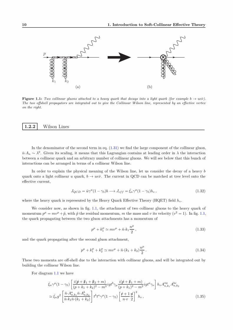
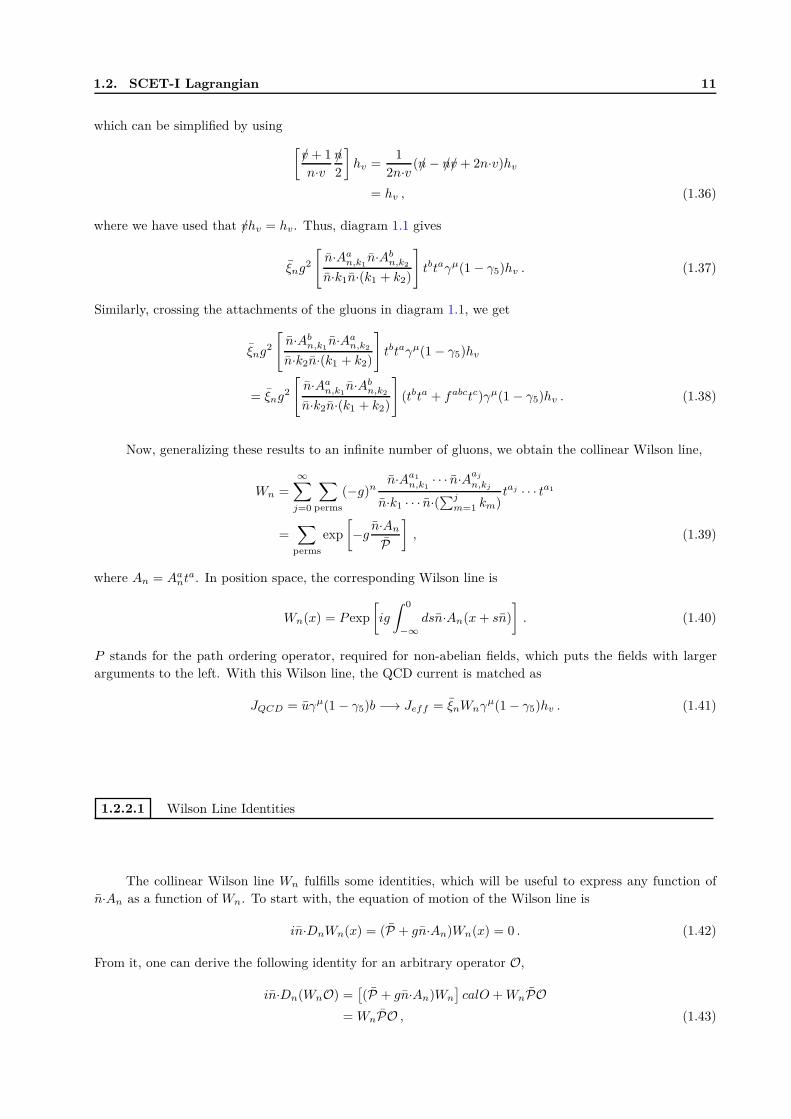
Figure 1.1: Two collinear gluons attached to a heavy quark that decays into a light quark (for example b → ueν).The two offshell propagators are integrated out to give the Collinear Wilson line, represented by an effective vertexon the right.
1.2.2 Wilson Lines
In the denominator of the second term in eq. (1.31) we find the large component of the collinear gluon,
n·An ∼ λ0. Given its scaling, it means that this Lagrangian contains at leading order in λ the interaction
between a collinear quark and an arbitrary number of collinear gluons. We will see below that this bunch of
interactions can be arranged in terms of a collinear Wilson line.
In order to explain the physical meaning of the Wilson line, let us consider the decay of a heavy b
quark onto a light collinear u quark, b → ueν. The current in QCD can be matched at tree level onto the
effective current,
JQCD = uγµ(1 − γ5)b −→ Jeff = ξnγµ(1 − γ5)hv , (1.32)
where the heavy quark is represented by the Heavy Quark Effective Theory (HQET) field hv.
We consider now, as shown in fig. 1.1, the attachment of two collinear gluons to the heavy quark of
momentum pµ = mvµ + p, with p the residual momentum, m the mass and v its velocity (v2 = 1). In fig. 1.1,
the quark propagating between the two gluon attachments has a momentum of
pµ + kµ1 ≃ mvµ + n·k1
nµ
2, (1.33)
and the quark propagating after the second gluon attachment,
pµ + kµ1 + kµ
2 ≃ mvµ + n·(k1 + k2)nµ
2. (1.34)
These two momenta are off-shell due to the interaction with collinear gluons, and will be integrated out by
building the collinear Wilson line.
For diagram 1.1 we have
ξnγµ(1 − γ5)
[
i(p/+ k/1 + k/2 +m)
(p+ k1 + k2)2 − m2igtbγµ
i(p/+ k/1 +m)
(p+ k1)2 −m2igtaγν
]
hvAaµn,k1
Abνn,k2
≃ ξng2
[
n·Aan,k1
n·Abn,k2
n·k1n·(k1 + k2)
]
tbtaγµ(1 − γ5)
[
v/ + 1
n·vn/
2
]2
hv , (1.35)
1.2. SCET-I Lagrangian 11
which can be simplified by using
[
v/ + 1
n·vn/
2
]
hv =1
2n·v (n/ − n/v/+ 2n·v)hv
= hv , (1.36)
where we have used that v/hv = hv. Thus, diagram 1.1 gives
ξng2
[
n·Aan,k1
n·Abn,k2
n·k1n·(k1 + k2)
]
tbtaγµ(1 − γ5)hv . (1.37)
Similarly, crossing the attachments of the gluons in diagram 1.1, we get
ξng2
[
n·Abn,k1
n·Aan,k2
n·k2n·(k1 + k2)
]
tbtaγµ(1 − γ5)hv
= ξng2
[
n·Aan,k1
n·Abn,k2
n·k2n·(k1 + k2)
]
(tbta + fabctc)γµ(1 − γ5)hv . (1.38)
Now, generalizing these results to an infinite number of gluons, we obtain the collinear Wilson line,
Wn =
∞∑
j=0
∑
perms
(−g)nn·Aa1
n,k1· · · n·Aaj
n,kj
n·k1 · · · n·(∑j
m=1 km)taj · · · ta1
=∑
perms
exp
[
−g n·An
P
]
, (1.39)
where An = Aant
a. In position space, the corresponding Wilson line is
Wn(x) = P exp
[
ig
∫ 0
−∞
dsn·An(x+ sn)
]
. (1.40)
P stands for the path ordering operator, required for non-abelian fields, which puts the fields with larger
arguments to the left. With this Wilson line, the QCD current is matched as
JQCD = uγµ(1 − γ5)b −→ Jeff = ξnWnγµ(1 − γ5)hv . (1.41)
1.2.2.1 Wilson Line Identities
The collinear Wilson line Wn fulfills some identities, which will be useful to express any function of
n·An as a function of Wn. To start with, the equation of motion of the Wilson line is
in·DnWn(x) = (P + gn·An)Wn(x) = 0 . (1.42)
From it, one can derive the following identity for an arbitrary operator O,
in·Dn(WnO) =[
(P + gn·An)Wn
]
calO +WnPO= WnPO , (1.43)
12 1. Introduction to Soft-Collinear Effective Theory
from which we obtain the operator identities
in·DnWn = WnP ,
in·Dn = WnPW †n ,P = W †nin·DnWn ,
1
in·Dn= W †n
1
PWn ,
1
P= Wn
1
in·DnW †n . (1.44)
Thus, any function f(P + gn·An) = f(in·Dn), which has an expansion∑
m am(in·Dn)m, can be expressed
as
f(P + gn·An) =∑
m
am(WnPW †n)m
= Wn
[
∑
m
amPm
]
W †n
= Wnf(P)W †n . (1.45)
With the relations above, the collinear quark Lagrangian in eq. (1.31) can be written as
L(0)nq = ξn,pl
(
in·D + iD/n⊥W†n
1
PWniD/n⊥
)
n/
2ξn,pl
. (1.46)
1.2.3 Collinear Gluon Lagrangian
Let us start from the QCD gluon Lagrangian,
L = −1
2tr {FµνFµν} +
1
αtr{
(i∂µAµ)2}
+ 2tr {ci∂µiDµc} , (1.47)
where Fµν = ig [Dµ, Dν ]. Expanding the covariant derivative and keeping the leading order terms,
iDµ ≃ (P + gn·An)nµ
2+ (Pµ
⊥ + gAµn⊥) + (in·∂ + gn·An + gn·Aus)
nµ
2
≡ iDµ , (1.48)
and hence we will have usoft gluons in the collinear gluon Lagrangian as well. The gauge fixing and ghost
terms should fix the gauge for collinear gluons only, and not for usoft gluons. Hence, we need them to be
covariant with respect to Aus, and this forces us to replace i∂µ by iDµus in the Lagrangian, where
iDµus ≡ P nµ
2+ Pµ
⊥ + in·∂ nµ
2+ gn·Aus
nµ
2. (1.49)
Notice that we have used only the component n·Aus, since it is the one that appears in the Lagrangian at
leading order. The resulting collinear gluon Lagrangian is
L(0)ng =
1
2g2tr{
[iDµ, iDµ]2}
+1
αtr{
[iDµus, Anµ]2
}
+ 2tr {cn[iDµus, [iDµ, cn]]} . (1.50)
1.2. SCET-I Lagrangian 13
p
µ1 , a1 µ2, a2 µn, an
k1 k2 kn + perms.
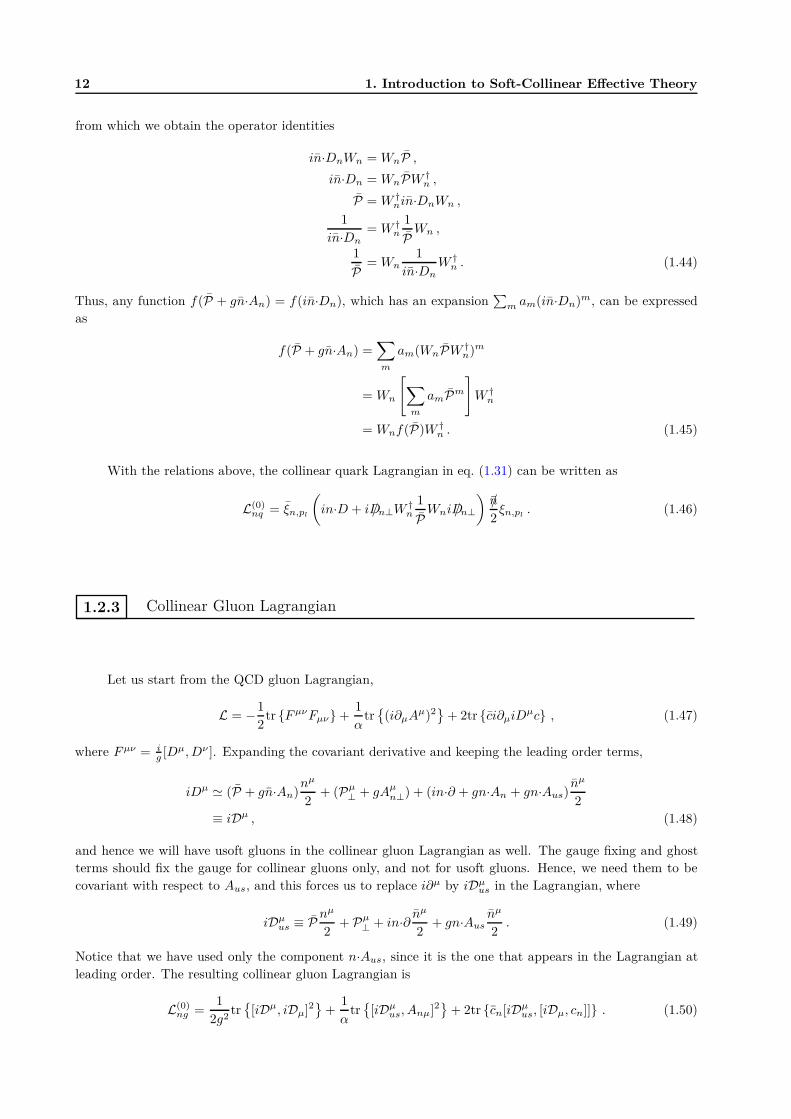
Figure 1.2: An arbitrary number of usoft gluons coupled to a collinear quark, giving rise to the usoft Wilson lineYn.
1.2.4 Ultrasoft Lagrangian
The leading order Lagrangian for ultrasoft quarks and gluons can be obtained directly from the QCD
Lagrangian where all fields are ultrasoft. Thus,
L(0)us = ψusiD/usψus − 1
2tr{
Fµνus F
usµν
}
+1
αustr{
(i∂µAµus)2
}
+ 2tr {cusi∂µiDµuscus} , (1.51)
where iDµus = i∂µ +gAµ
us. Notice that all terms in this Lagrangian scale as λ8, consistently with the measure
for ultrasoft fields, which scales as d4 ∼ λ−8. Thus, the leading order action scales as λ0, as required
by the standard choice that we also adopt. The gauge fixing parameter αus is independent from the one
that appears in the collinear gluon Lagrangian, since there are independent collinear and ultrasoft gauge
transformations.
1.2.5 Usoft Interactions with Collinear Quarks and Gluons
In this section we will see that usoft gluons and collinear particles can be decoupled by using two new
Wilson lines, in such a way that their interactions explicitly disappear from the collinear Lagrangians at
leading order in λ. At higher orders different interactions appear in the Lagrangian and they cannot be
integrated out.
In fig. 1.2 we can see the coupling of an arbitrary number of usoft gluons to a collinear quark. Following
the same steps as for the collinear Wilson lines, the matching with all these couplings gives us
ξn = Yn ξ(0)n,p , (1.52)
where the usoft Wilson line is
Yn = 1 +
∞∑
j=1
∑
perms
(−g)j
j!
n·Aa1us · · ·n·Aaj
us
n·k1 · · ·n·(∑j
i=1 ki)taj · · · ta1 . (1.53)
Doing the Fourier transform we obtain
Yn(x) = P exp
(
ig
∫ 0
−∞
ds n·Aaus(x+ ns)ta
)
. (1.54)
In eq. (1.52) ξ(0)n does not interact with usoft gluons, since these couplings are contained in the usoft Wilson
line Yn.
In a similar way we can calculate the contribution from the coupling of an arbitrary number of usoft
14 1. Introduction to Soft-Collinear Effective Theory
p µ, aν, b
µ1, a1 µ2, a2 µn, an
k1 k2 kn+ perms.
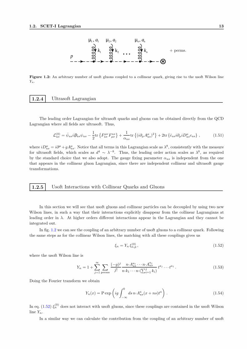
Figure 1.3: An arbitrary number of usoft gluons coupled to a collinear gluon, giving rise to the usoft Wilson lineYn.
gluon to a collinear gluon, fig. 1.3. We obtain the following,
Aaµn = Yab A(0) bµ
n , (1.55)
with
Yabn = δab +
∞∑
j=1
∑
perms
(ig)j
j!
n·Aa1us · · · n·Aaj
us
n·k1 · · · n·(∑ji=1 ki)
fajacj−1 · · · fa2c2c1fa1c1b . (1.56)
As in the previous case, A(0)n does not couple to usoft gluons. Doing again the Fourier transform, which is
related to the one of Yn(x) but in the adjoint representation,
Yabn (x) =
[
P exp
(
ig2
∫ 0
−∞
ds n·Aeus(x+ ns)T e
)]ab
, (1.57)
with (T e)ab = −ifeab.
The adjoint representation is related to the fundamental one by YntaY †n = Ybatb, and this allows us to
relate Aµn with A
(0) µn and cn with c
(0)n ,
Aµn = Abµ
n tb = A(0)aµn Yba
n tb = A(0)aµn Yn t
aY †n = YnA(0)µn Y †n ,
cn = cant
a = c(0)bn Yab
n ta = Y c(0)n Y †n . (1.58)
On the other hand, it can be shown as well that Wn = YnW(0)n Y †n .
Now we can prove what was introduced at the beginning of this section, i.e., the usoft particles can be
decoupled from collinear ones at the level of the Lagrangian at leading order, both for collinear quark and
gluon Lagrangians. With the previous redefinitions of fields, we can write L(0)nq as
L(0)nq = ξn,pl
(
in·D + iD/n⊥W†n
1
PWniD/n⊥
)
n/
2ξn,pl
= ξ(0)n,p−lY
†n
{
in·D + gYnn·A(0)n Y †n +
(
P/⊥ + YngA/(0)n⊥Y
†n
)
YnW(0)n Y †n
1
P
× YnW(0)†n Y †n
(
P/⊥ + YngA/(0)n⊥Y
†n
)
}
n/
2Ynξ
(0)n,pl
}
= ξ(0)n,pl
{
Y †n in·DYn + gn·A(0)n
+(
P/⊥ + gA/(0)n⊥
)
W (0)n
1
PW (0)†
n
(
P/⊥ + gA/(0)n⊥
)
}
n/
2ξ(0)
n,pl, (1.59)
where we have used that Yn commutes with P/⊥. Using now that n·DYn = 0, we can see that Y †nn·DYn = n·∂,
1.3. Symmetries in SCET-I 15
and thus the Lagrangian for collinear quarks becomes
L(0)nq = ξ(0)
n,pl
{
in·∂ + gn·A(0)n +
(
P/⊥ + gA/(0)n⊥
)
W (0)n
1
PW (0)†
n
(
P/⊥ + gA/(0)n⊥
)
}
n/
2ξ(0)
n,pl, (1.60)
which is completely independent of usoft gluons.
Following similar steps we can decouple usoft gluons from collinear gluons. Using iDµ + gAµn =
Yn(iDµ(0) + gA
(0)µn )Y †n we can write
L(0)ng =
1
2g2tr
{
[
iDµ(0) + gA(0)µ
n , iDν(0) + gA(0)ν
n
]
}2
+1
αtr
{
[
iD(0)µ , A(0)µ
n
]
}2
+ 2tr
{
c(0)n
[
iD(0)µ ,[
iDµ(0) + gA(0)µ
n , c(0)n
]]
}
, (1.61)
where iDµ(0) = P nµ
2 + Pµ⊥ + in·∂ nµ
2 .
1.3 Symmetries in SCET-I
In this section we introduce the gauge symmetry and the reparameterization invariance. We will see
that gauge symmetry in SCET is similar to the one in full QCD, but splitting the gauge field in two fields,
collinear and ultrasoft. The reparameterization invariance comes from Lorentz invariance, which is broken
when we choose the light-cone coordinates, and thus will be applied in the two collinear sectors independently.
These symmetries restrict the operators we can consider in SCET [36].
1.3.1 Gauge Symmetry in SCET
Let us consider a general gauge transformation in full QCD,
U(x) = exp[iαata] , (1.62)
which acts on a field as
ψ(x) −→ U(x)ψ(x) , (1.63)
or equivalently as
ψ(p) −→∫
dqU(p− q)ψ(q) . (1.64)
In SCET we need the gauge transformation to be consistent with power counting, and thus only two sets of
transformation are allowed, collinear and ultrasoft:
Un(x) : i∂µUn(x) ∼ Q(1, λ2, λ)Un(x) ,
Uus(x) : i∂µUus(x) ∼ Q(λ2, λ2, λ2)Uus(x) . (1.65)
16 1. Introduction to Soft-Collinear Effective Theory
Then, the set of collinear gauge transformations are
ξn(x) −→ Un(x)ξn(x) ,
Aµn(x) −→ Un(x)
(
Aµn(x) +
i
gDµ
us
)
U †n(x) ,
ψus(x) −→ ψus(x) ,
Aµus(x) −→ Aµ
us(x) . (1.66)
And the set of ultrasoft transformations,
ξn(x) −→ Uus(x)ξn(x) ,
Aµn(x) −→ Uus(x)Aµ
n(x)U †us(x) ,
ψus(x) −→ Uus(x)ψus(x) ,
Aµus(x) −→ Uus(x)
(
Aµus(x) +
i
g∂µ
)
U †us(x) . (1.67)
Finally, the collinear Wilson line transforms as Wn(x) → Un(x)Wn(x) under collinear gauge transfor-
mations and as Wn(x) → Uus(x)Wn(x)U †us(x) under ultrasoft gauge transformations.
1.3.2 Reparameterization Invariance SCET
The requirements we asked to our light-cone momenta were
n2 = n2 = 0 , n·n = 2 . (1.68)
Therefore, there are three sets of allowed transformations we can apply to a given pair of light-cone vectors
and still obey the above equation:
• Type I:
nµ −→ nµ + εµn⊥
nµ −→ nµ (1.69)
• Type II:
nµ −→ nµ
nµ −→ nµ + εµn⊥ (1.70)
• Type III:
nµ −→ eαnµ
nµ −→ e−αnµ (1.71)
Type I and II transformations are infinitesimal, and type III can be made infinitesimal by expanding in α.
Since these sets of transformations must leave a collinear particle as collinear, we can derive the scaling of the
parameters by considering the transformation of a collinear particle of momentum p ∼ (1, λ2, λ). Considering
type I,
(n·p, n·p, p⊥) ∼ (1, λ2, λ) −→ (n·p, n·p+ ǫn⊥·p⊥, p⊥) ∼ (1, λ2, λ) , (1.72)
1.4. SCET-II 17
from which we can see that ǫn⊥ ∼ λ, so it is constrained by power counting. Considering now type II
transformation we have,
(n·p, n·p, p⊥) ∼ (1, λ2, λ) −→ (n·p+ εn⊥·p⊥, n·p, p⊥) ∼ (1, λ2, λ) , (1.73)
which does not impose any scaling over εn⊥, which can be as large as we want. Finally, type III transforma-
tions do not impose any restriction over α, which again can be as large as we want.
1.4 SCET-II
In SCET-II the relevant degrees of freedom are soft and collinear, which scale as
pn ∼ Q(1, η2, η)
ps ∼ Q(η, η, η) , (1.74)
with η = ΛQCD/Q. Notice that soft momenta scale as the ultrasoft momenta in SCET-I, given that pus ∼Q(λ2, λ2, λ2) with λ =
√
ΛQCD/Q. However collinear momenta scale different from SCET-I. It is also worth
noticing that while one can have interactions between collinear and ultrasoft modes, the soft modes cannot
couple to collinear particles, because they would be driven off-shell:
pn + ps = Q(1, η2, η) +Q(η, η, η) = Q(1, η, η) . (1.75)
This crucial difference with SCET-I makes the Lagrangian of SCET-II much simpler to derive, because we
have right from the start a clear separation of collinear and soft modes, which cannot interact with each
other. Thus, the Lagrangian for SCET-II is
L(0)SCET−II = L(0)
nq + L(0)ng + L(0)
s , (1.76)
where the collinear Lagrangians are the same as for SCET-I and the soft Lagrangian is analogous to the
ultrasoft one for SCET-I where we replace ultrasoft modes by soft modes.
For a given process, the identification of the relevant soft and (anti)collinear modes depends on the
chosen frame. Given that soft and collinear modes have the same invariant mass, Q2η2, they can be dis-
tinguished just by their relative rapidities. Thus, one can perform a boost and transform soft modes into
(anti)collinear modes, and vice versa. However, the physical process being described is exactly the same.
This does not happen in SCET-I, where the mass of collinear particles is Q2λ2, while for ultrasoft particles
it is Q2λ4.
Since the soft modes in SCET-II are basically the same as ultrasoft modes in SCET-I, the matching
between these two theories is done by replacing ultrasoft Wilson lines by soft Wilson lines, Yn(n) → Sn(n).
Notice that the functional form of soft Wilson lines is exactly the same as ultrasoft Wilson lines.
1.5 Factorization of the Quark Form Factor
Once the SCET machinery has been introduced, let us illustrate its application by factorizing the
simplest quantity, the electromagnetic Quark Form Factor, to first order in αs. We show how the hard
matching coefficient (Wilson coefficient) is obtained by performing an explicit perturbative calculation, for
which the effective theory has to reproduce the full QCD infrared divergences. Furthermore, this calculation
will serve to clarify some relevant issues, as the double counting and the role of the zero-bin to deal with it,
the necessity to regulate consistently the divergences in full QCD and the effective theory and the difference
between ultraviolet (UV), infrared (IR) and rapidity divergences.
18 1. Introduction to Soft-Collinear Effective Theory
p
p
(a) (b) (c)
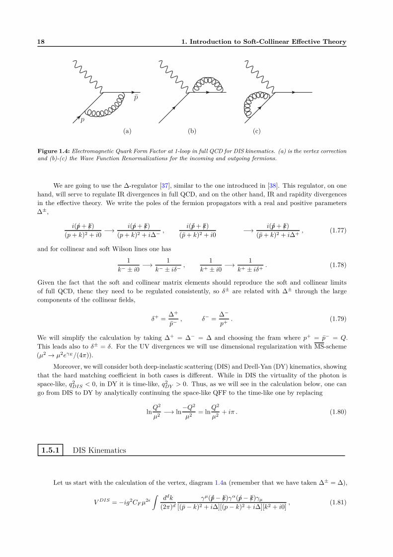
Figure 1.4: Electromagnetic Quark Form Factor at 1-loop in full QCD for DIS kinematics. (a) is the vertex correctionand (b)-(c) the Wave Function Renormalizations for the incoming and outgoing fermions.
We are going to use the ∆-regulator [37], similar to the one introduced in [38]. This regulator, on one
hand, will serve to regulate IR divergences in full QCD, and on the other hand, IR and rapidity divergences
in the effective theory. We write the poles of the fermion propagators with a real and positive parameters
∆±,
i(p/+ k/)
(p+ k)2 + i0−→ i(p/+ k/)
(p+ k)2 + i∆−,
i(p/+ k/)
(p+ k)2 + i0−→ i(p/+ k/)
(p+ k)2 + i∆+, (1.77)
and for collinear and soft Wilson lines one has
1
k− ± i0−→ 1
k− ± iδ−,
1
k+ ± i0−→ 1
k+ ± iδ+. (1.78)
Given the fact that the soft and collinear matrix elements should reproduce the soft and collinear limits
of full QCD, thenc they need to be regulated consistently, so δ± are related with ∆± through the large
components of the collinear fields,
δ+ =∆+
p−, δ− =
∆−
p+. (1.79)
We will simplify the calculation by taking ∆+ = ∆− = ∆ and choosing the fram where p+ = p− = Q.
This leads also to δ± = δ. For the UV divergences we will use dimensional regularization with MS-scheme
(µ2 → µ2eγE/(4π)).
Moreover, we will consider both deep-inelastic scattering (DIS) and Drell-Yan (DY) kinematics, showing
that the hard matching coefficient in both cases is different. While in DIS the virtuality of the photon is
space-like, q2DIS < 0, in DY it is time-like, q2
DY > 0. Thus, as we will see in the calculation below, one can
go from DIS to DY by analytically continuing the space-like QFF to the time-like one by replacing
lnQ2
µ2−→ ln
−Q2
µ2= ln
Q2
µ2+ iπ . (1.80)
1.5.1 DIS Kinematics
Let us start with the calculation of the vertex, diagram 1.4a (remember that we have taken ∆± = ∆),
V DIS = −ig2CFµ2ǫ
∫
ddk
(2π)d
γµ(p/− k/)γα(p/− k/)γµ
[(p− k)2 + i∆][(p− k)2 + i∆][k2 + i0], (1.81)
1.5. Factorization of the Quark Form Factor 19
where ddk = 12dk
+dk−dd−2~k⊥. Notice that we are calculating the corrections to the electromagnetic current,
which can be written as
un(p)Oµ⊥un(p) = un(p)
n/n/
4Oµ⊥
n/n/
4un(p) , (1.82)
where Oµ⊥ corresponds to the particular Dirac structure relevant for a given diagram. Since the projectors
force the inner Oµ⊥ to be perpendicular to nµ and nµ, we can use them to simplify the Dirac structure. Thus,
the final relevant combination of terms we get after simplifying the numerator is:
[
2Q2 + 2(p− k)2 + 2(p− k)2 − 2(1 + ǫ)k2]
γα⊥ − 4(1 − ǫ)k/⊥k
α⊥ , (1.83)
and we can write the contribution of the vertex as
V DIS =[
2Q2I1 + 2I2(p) + 2I2(p) − 2(1 + ǫ)I3
]
γα⊥ − 4(1 − ǫ)Iα
4 . (1.84)
The necessary integrals in the Q2 → ∞ limit are (notice that p2 = p2 = 0 and pp = Q2/2):
I1 = −ig2CFµ2ǫ
∫
ddk
(2π)d
1
[(p− k)2 + i∆][(p− k)2 + i∆][k2 + i0]
= −ig2CFµ2ǫ
∫ 1
0
dx dy
∫
ddk
(2π)d
2y
[k2 − 2k(xyp+ (1 − x)yp) + yi∆]3
= −αsCF
2π
1
Q2
1
2ln2 −i∆
Q2, (1.85)
which we have multiplied and divided by Q2 to expand it around Q2 → ∞.
The integral I2 is
I2 = −ig2CFµ2ǫ
∫
ddk
(2π)d
1
[(p− k)2 + i∆][k2 + i0]
= −ig2CFµ2ǫ
∫ 1
0
dx
∫
ddk
(2π)d
1
(k2 − 2kxp+ xi∆)2
=αsCF
2π
(
1
2εUV+
1
2− 1
2ln
−i∆µ2
)
. (1.86)
The calculation of I3 gives us
I3 = −ig2CFµ2ǫ
∫
ddk
(2π)d
1
[(p− k)2 + i∆][(p− k)2 + i∆]
= −ig2CFµ2ǫ
∫ 1
0
dx
∫
ddk
(2π)d
1
(k2 − 2k(xp+ (1 − x)p) + i∆)2
=αsCF
2π
(
1
2εUV+ 1 − 1
2lnQ2
µ2
)
, (1.87)
which does not have IR divergences.
20 1. Introduction to Soft-Collinear Effective Theory
Finally, we have
Iα4 = −ig2CFµ
2ǫ
∫
ddk
(2π)d
k/⊥kα⊥
[(p− k)2 + i∆][(p− k)2 + i∆][k2 + i0]=
= −ig2CFµ2ǫ
∫ 1
0
dy dx
∫
ddk
(2π)d
2y k/⊥kα⊥
[k2 − 2k(xyp+ (1 − x)yp) + yi∆]3
(We take only the contribution ∝ γα⊥ and define l = k − xyp− (1 − x)yp)
= −ig2CFγα⊥
d− 2µ2ǫ
∫ 1
0
dy dx
∫
ddl
(2π)d
y l2⊥[l2 − xy2(1 − x)Q2 + yi∆]
3
=αsCF
2π
1
8
(
1
εUV+ 3 − ln
Q2
µ2
)
, (1.88)
which again does not have any IR divergence.
Combining the results above, the final result for the vertex is:
V DIS =[
2Q2I1 + 2I2(p) + 2I2(p) − 2(1 + ǫ)I3
]
γα⊥ − 4(1 − ǫ)Iα
4
=αsCF
2πγα⊥
(
1
2εUV− ln2 −i∆
Q2− 2ln
−i∆µ2
+3
2lnQ2
µ2− 2
)
(1.89)
For the WFR, diagrams 1.4b and 1.4c, we have to compute the following integral:
Iw = −g2CFµ2ǫ
∫
ddk
(2π)d
γµ(p/− k/)γµ
[(p− k)2 + i∆][k2 + i0], (1.90)
where the numerator can be simplified as
γµ(p/ − k/)γµ = −(d− 2)(p/− k/) . (1.91)
Then we have
Iw = −g2CFµ2ǫ
∫
ddk
(2π)d
−(d− 2)(p/− k/)
[(p− k)2 + i∆][k2 + i0]
= ip/αsCF
2π
(
1
2εUV+
1
4− 1
2ln
−i∆µ2
)
, (1.92)
which contributes to the QFF with − 12Iw(p)/(ip/).
Thus, the final result for the Quark Form Factor calculated in QCD, with the ∆-regulator and for DIS
kinematics, is
〈p| JµQCD |p〉DIS
= V DIS − 1
2
Iw(p)
ip/γα⊥ − 1
2
Iw(p)
ip/γα⊥ =
= γα⊥
[
1 +αsCF
2π
(
−ln2 −i∆Q2
− 3
2ln
−i∆Q2
− 9
4
)]
(1.93)
Our aim now is to match the full QCD electromagnetic current onto the SCET one,
JµQCD = ψγµψ −→ Jµ
SCET = ξnWnY†
nγµYnW
†nξn , (1.94)
1.5. Factorization of the Quark Form Factor 21
(a) (b) (c)
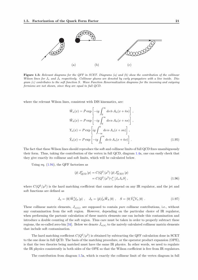
Figure 1.5: Relevant diagrams for the QFF in SCET. Diagrams (a) and (b) show the contribution of the collinearWilson lines for Jn and Jn respectively. Collinear gluons are denoted by curly propagators with a line inside. Dia-gram (c) contributes to the soft function S. Wave Function Renormalization diagrams for the incoming and outgoingfermions are not shown, since they are equal to full QCD.
where the relevant Wilson lines, consistent with DIS kinematics, are:
Wn(x) = P exp
[
−ig∫ ∞
0
ds n·An(x+ ns)
]
,
Wn(x) = P exp
[
−ig∫ ∞
0
ds n·An(x+ ns)
]
,
Yn(x) = P exp
[
ig
∫ 0
−∞
ds n·As(x+ sn)
]
,
Yn(x) = P exp
[
−ig∫ ∞
0
ds n·As(x + ns)
]
. (1.95)
The fact that these Wilson lines should reproduce the soft and collinear limits of full QCD fixes unambiguously
their form. Thus, taking the contribution of the vertex in full QCD, diagram 1.4a, one can easily check that
they give exactly its collinear and soft limits, which will be calculated below.
Using eq. (1.94), the QFF factorizes as
〈p| JµQCD |p〉 = C(Q2/µ2) 〈p|Jµ
SCET |p〉= C(Q2/µ2)γµ
⊥ [JnJnS] , (1.96)
where C(Q2/µ2) is the hard matching coefficient that cannot depend on any IR regulator, and the jet and
soft functions are defined as
Jn = 〈0| W †nξn |p〉 , Jn = 〈p| ξnWn |0〉 , S = 〈0| Y †nYn |0〉 . (1.97)
These collinear matrix elements, Jn(n), are supposed to contain pure collinear contributions, i.e., without
any contamination from the soft region. However, depending on the particular choice of IR regulator,
when performing the partonic calculation of these matrix elements one can include this contamination and
introduce a double counting of the soft region. Thus care must be taken in order to properly subtract these
regions, the so-called zero-bin [34]. Below we denote Jn(n) to the naively calculated collinear matrix elements
that include soft contamination.
The hard matching coefficient C(Q2/µ2) is obtained by subtracting the QFF calculation done in SCET
to the one done in full QCD. The basis of the matching procedure, or the operator product expansion (OPE),
is that the two theories being matched must have the same IR physics. In other words, we need to regulate
the IR physics consistently in both sides of the OPE so that the Wilson coefficient is free from IR regulators.
The contribution from diagram 1.5a, which is exactly the collinear limit of the vertex diagram in full
22 1. Introduction to Soft-Collinear Effective Theory
QCD when k ∼ (1, λ2, λ), is
J(1.5a)n1 = −2ig2CFµ
2ǫ
∫
ddk
(2π)d
p+ + k+
[k+ + iδ][(p+ k)2 + i∆][k2 + i0]. (1.98)
The poles in k− are
k−1 =−k2⊥ − i∆
k+ + p+, k−2 =
−k2⊥ − i0
k+. (1.99)
When k+ > 0, both poles lie in the lower complex half-plane and we can close the contour through the
upper half-plane, giving zero for the integral. When k+ < −p+, both poles lie in the upper half-plane and
we can close the contour through the lower half-plane, giving again zero for the integral. However, when
−p+ < k+ < 0, we choose to close the contour through the upper half-plane, thus picking the pole k−2 .
Setting k+ = zp+ we get
J (1.5a)n = 2αsCFµ
2ε
∫ 0
−1
dz p+
∫
dd−2k⊥(2π)d−2
p+ + zp+
(zp+ + iδ)(−p+k2⊥ + izp+∆)
. (1.100)
Doing the k⊥ integral we get
J (1.5a)n = −αsCF
2π(4πµ2)εΓ(ε)(−i∆)−ε
∫ 1
0
dz(1 − z)z−ε
z − iδ/p+. (1.101)
In this result, the k⊥ → ∞ is regulated by ε and the limit k⊥ → 0 is regulated by ∆. Finally, performing
the integral over z we get
J (1.5a)n = −αsCF
2π(4πµ2)εΓ(ε)(−i∆)−ε
[
−1 − ε+επ2
6− ln
−iδp+
+ε
2ln2 −iδ
p+
]
=αsCF
2π
[
1
εUV+
1
εUVln
−i∆Q2
+ 1 − π2
6− 1
2ln2 −i∆
Q2− ln
−i∆µ2
−ln−i∆µ2
ln−i∆Q2
]
, (1.102)
where we have set δ/p+ = ∆/Q2, consistently with eq. (1.79).
The soft function at O(αs) is given by diagram 1.5c, again corresponds to the soft limit of the vertex
in full QCD when k ∼ (λ2, λ2, λ2),
S(1.5c)1 = −2ig2CFµ
2ε
∫
ddk
(2π)d
1
[k+ + iδ][k− + iδ][k2 + i0]
=αsCF
2π(4πµ2)εΓ(ε)
∫ 0
−∞
dk−(k−iδ)−ε
k− + iδ
=αsCF
2π(4πµ2)εΓ(ε)(iδiδ)−επcsc(πε)
=αsCF
2π
[
− 1
ε2UV
+1
εUVln
(−i∆)(−i∆)
Q2µ2− 1
2ln2 (−i∆)(−i∆)
Q2µ2− π2
4
]
. (1.103)
The contribution to Jn from diagram 1.5b is analogous to eq. (1.102),
J(1.5b)n =
αsCF
2π
[
1
εUV+
1
εUVln
−i∆Q2
+ 1 − π2
6− 1
2ln2 −i∆
Q2− ln
−i∆µ2
−ln−i∆µ2
ln−i∆Q2
]
, (1.104)
given the fact that we have set ∆± = ∆.
1.5. Factorization of the Quark Form Factor 23
In order to get the contribution of the pure collinear matrix elements Jn, we should subtract to eq. (1.98)
its contamination from the soft region. Taking k ∼ Q(λ2, λ2, λ2) in the integrand, we can see that the integral
is equal to the soft function. The same applies to Jn and Jn. Thus all we need to do is subtract the soft
function from the factorization formula instead of adding it,
〈p| JµQCD |p〉 = C(Q2/µ2)γµ
⊥
[
JnJnS−1]
. (1.105)
Then, combing the previous results, the vertex in the effective theory at O(αs) is
V DISSCET = γα
⊥
[
J (1.5a)n + J
(1.5b)n − S(1.5c)
]
= γα⊥
αsCF
2π
[
1
ε2UV
+2
εUV− 1
εUVlnQ2
µ2− ln2 −i∆
Q2− 2ln
−i∆µ2
+3
2lnQ2
µ2− 2
+1
2ln2Q
2
µ2− 3
2lnQ2
µ2+ 4 − π2
12
]
(1.106)
The WFR diagrams are the same in full QCD as in the effective theory, so the QFF in SCET is
〈p| JµSCET |p〉 = γα
⊥
αsCF
2π
[
1
ε2UV
+3
2εUV− 1
εUVlnQ2
µ2
−ln2 −i∆Q2
− 3
2ln
−i∆Q2
− 9
4
+1
2ln2Q
2
µ2− 3
2lnQ2
µ2+ 4 − π2
12
]
(1.107)
Comparing this result with the QFF in full QCD calculated before, we can see that the IR poles (second
line) are the same. This is a must in any OPE, where by construction the theories above and below the
matching scale (Q in our case) have to contain the same IR physics. Of course, in order to see this fact at
the level of the partonic calculation it is necessary to regulate consistently the IR in the two theories.
Finally, ignoring the UV poles which do not have to be considered while performing an OPE, we obtain
the matching coefficient,
C(Q2/µ2) = 1 +αsCF
2π
[
−1
2ln2Q
2
µ2+
3
2lnQ2
µ2− 4 +
π2
12
]
, (1.108)
which coincides with the one derived for the first time in [39].
1.5.2 DY Kinematics
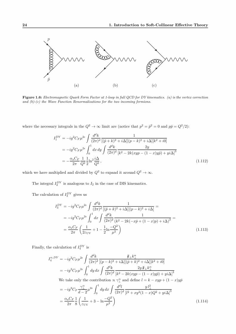
The vertex for Drell-Yan kinematics in fig. 1.6a is:
V DY = +ig2CFµ2ǫ
∫
ddk
(2π)d
γµ(p/+ k/)γα(p/ − k/)γµ
[(p+ k)2 + i∆][(p− k)2 + i∆][k2 + i0], (1.109)
This integral can be obtained from the analogous one in DIS kinematics just by replacing p → −p.The simplification of the numerator gives
[
−2Q2 + 2(p+ k)2 + 2(p− k)2 − 2(1 + ǫ)k2]
γα⊥ − 4(1 − ǫ)k/⊥k
α⊥ . (1.110)
Then, we can write the contribution of the vertex as
V DY =[
−2Q2IDY1 + 2IDY
2 (p) + 2IDY2 (p) − 2(1 + ǫ)IDY
3
]
γα⊥ − 4(1 − ǫ)Iα
4 , (1.111)
24 1. Introduction to Soft-Collinear Effective Theory
p
p
(a) (b) (c)
Figure 1.6: Electromagnetic Quark Form Factor at 1-loop in full QCD for DY kinematics. (a) is the vertex correctionand (b)-(c) the Wave Function Renormalizations for the two incoming fermions.
where the necessary integrals in the Q2 → ∞ limit are (notice that p2 = p2 = 0 and pp = Q2/2):
IDY1 = −ig2CFµ
2ǫ
∫
ddk
(2π)d
1
[(p+ k)2 + i∆][(p− k)2 + i∆][k2 + i0]
= −ig2CFµ2ǫ
∫ 1
0
dx dy
∫
ddk
(2π)d
2y
[k2 − 2k(xyp− (1 − x)yp) + yi∆]3
= −αsCF
2π
1
Q2
1
2ln2 i∆
Q2, (1.112)
which we have multiplied and divided by Q2 to expand it around Q2 → ∞.
The integral IDY2 is analogous to I2 in the case of DIS kinematics.
The calculation of IDY3 gives us
IDY3 = −ig2CFµ
2ǫ
∫
ddk
(2π)d
1
[(p+ k)2 + i∆][(p− k)2 + i∆]=
= −ig2CFµ2ǫ
∫ 1
0
dx
∫
ddk
(2π)d
1
(k2 − 2k(−xp+ (1 − x)p) + i∆)2 =
=αsCF
2π
(
1
2εUV+ 1 − 1
2ln
−Q2
µ2
)
(1.113)
Finally, the calculation of IDY4 is
Iα,DY4 = −ig2CFµ
2ǫ
∫
ddk
(2π)d
k/⊥kα⊥
[(p− k)2 + i∆][(p+ k)2 + i∆][k2 + i0]
= −ig2CFµ2ǫ
∫ 1
0
dy dx
∫
ddk
(2π)d
2y k/⊥kα⊥
[k2 − 2k(xyp− (1 − x)yp) + yi∆]3
We take only the contribution ∝ γα⊥ and define l = k − xyp+ (1 − x)yp
= −ig2CFγα⊥
d− 2µ2ǫ
∫ 1
0
dy dx
∫
ddl
(2π)d
y l2⊥[l2 + xy2(1 − x)Q2 + yi∆]3
=αsCF
2π
1
8
(
1
εUV+ 3 − ln
−Q2
µ2
)
(1.114)
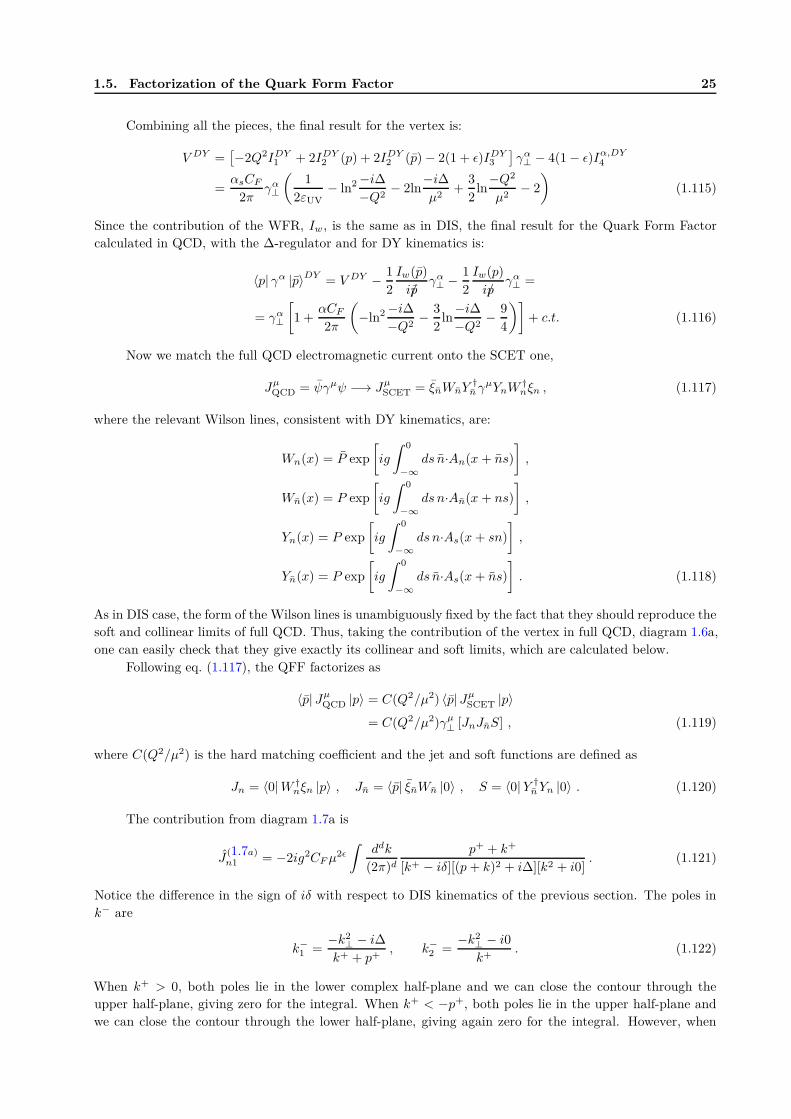
1.5. Factorization of the Quark Form Factor 25
Combining all the pieces, the final result for the vertex is:
V DY =[
−2Q2IDY1 + 2IDY
2 (p) + 2IDY2 (p) − 2(1 + ǫ)IDY
3
]
γα⊥ − 4(1 − ǫ)Iα,DY
4
=αsCF
2πγα⊥
(
1
2εUV− ln2 −i∆
−Q2− 2ln
−i∆µ2
+3
2ln
−Q2
µ2− 2
)
(1.115)
Since the contribution of the WFR, Iw , is the same as in DIS, the final result for the Quark Form Factor
calculated in QCD, with the ∆-regulator and for DY kinematics is:
〈p| γα |p〉DY= V DY − 1
2
Iw(p)
ip/γα⊥ − 1
2
Iw(p)
ip/γα⊥ =
= γα⊥
[
1 +αCF
2π
(
−ln2 −i∆−Q2
− 3
2ln
−i∆−Q2
− 9
4
)]
+ c.t. (1.116)
Now we match the full QCD electromagnetic current onto the SCET one,
JµQCD = ψγµψ −→ Jµ
SCET = ξnWnY†
nγµYnW
†nξn , (1.117)
where the relevant Wilson lines, consistent with DY kinematics, are:
Wn(x) = P exp
[
ig
∫ 0
−∞
ds n·An(x + ns)
]
,
Wn(x) = P exp
[
ig
∫ 0
−∞
ds n·An(x + ns)
]
,
Yn(x) = P exp
[
ig
∫ 0
−∞
ds n·As(x+ sn)
]
,
Yn(x) = P exp
[
ig
∫ 0
−∞
ds n·As(x+ ns)
]
. (1.118)
As in DIS case, the form of the Wilson lines is unambiguously fixed by the fact that they should reproduce the
soft and collinear limits of full QCD. Thus, taking the contribution of the vertex in full QCD, diagram 1.6a,
one can easily check that they give exactly its collinear and soft limits, which are calculated below.
Following eq. (1.117), the QFF factorizes as
〈p| JµQCD |p〉 = C(Q2/µ2) 〈p|Jµ
SCET |p〉= C(Q2/µ2)γµ
⊥ [JnJnS] , (1.119)
where C(Q2/µ2) is the hard matching coefficient and the jet and soft functions are defined as
Jn = 〈0|W †nξn |p〉 , Jn = 〈p| ξnWn |0〉 , S = 〈0|Y †nYn |0〉 . (1.120)
The contribution from diagram 1.7a is
J(1.7a)n1 = −2ig2CFµ
2ǫ
∫
ddk
(2π)d
p+ + k+
[k+ − iδ][(p+ k)2 + i∆][k2 + i0]. (1.121)
Notice the difference in the sign of iδ with respect to DIS kinematics of the previous section. The poles in
k− are
k−1 =−k2⊥ − i∆
k+ + p+, k−2 =
−k2⊥ − i0
k+. (1.122)
When k+ > 0, both poles lie in the lower complex half-plane and we can close the contour through the
upper half-plane, giving zero for the integral. When k+ < −p+, both poles lie in the upper half-plane and
we can close the contour through the lower half-plane, giving again zero for the integral. However, when
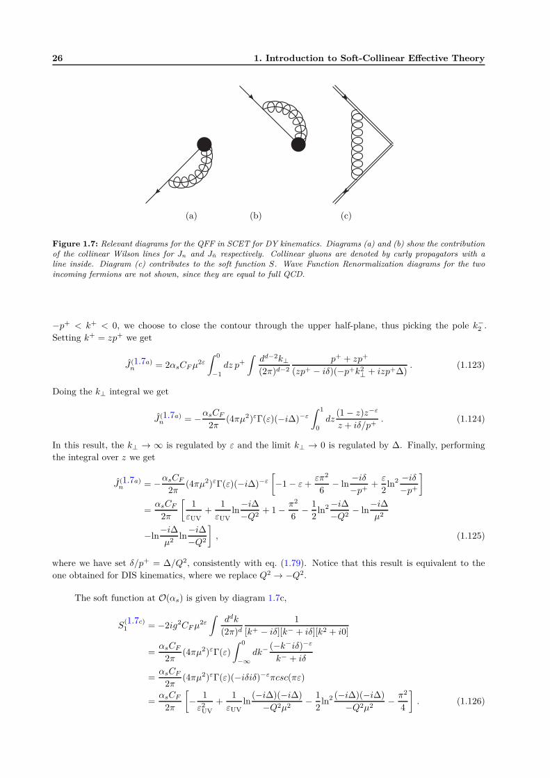
26 1. Introduction to Soft-Collinear Effective Theory
(a) (b) (c)
Figure 1.7: Relevant diagrams for the QFF in SCET for DY kinematics. Diagrams (a) and (b) show the contributionof the collinear Wilson lines for Jn and Jn respectively. Collinear gluons are denoted by curly propagators with aline inside. Diagram (c) contributes to the soft function S. Wave Function Renormalization diagrams for the twoincoming fermions are not shown, since they are equal to full QCD.
−p+ < k+ < 0, we choose to close the contour through the upper half-plane, thus picking the pole k−2 .
Setting k+ = zp+ we get
J (1.7a)n = 2αsCFµ
2ε
∫ 0
−1
dz p+
∫
dd−2k⊥(2π)d−2
p+ + zp+
(zp+ − iδ)(−p+k2⊥ + izp+∆)
. (1.123)
Doing the k⊥ integral we get
J (1.7a)n = −αsCF
2π(4πµ2)εΓ(ε)(−i∆)−ε
∫ 1
0
dz(1 − z)z−ε
z + iδ/p+. (1.124)
In this result, the k⊥ → ∞ is regulated by ε and the limit k⊥ → 0 is regulated by ∆. Finally, performing
the integral over z we get
J (1.7a)n = −αsCF
2π(4πµ2)εΓ(ε)(−i∆)−ε
[
−1 − ε+επ2
6− ln
−iδ−p+
+ε
2ln2 −iδ
−p+
]
=αsCF
2π
[
1
εUV+
1
εUVln
−i∆−Q2
+ 1 − π2
6− 1
2ln2 −i∆
−Q2− ln
−i∆µ2
−ln−i∆µ2
ln−i∆−Q2
]
, (1.125)
where we have set δ/p+ = ∆/Q2, consistently with eq. (1.79). Notice that this result is equivalent to the
one obtained for DIS kinematics, where we replace Q2 → −Q2.
The soft function at O(αs) is given by diagram 1.7c,
S(1.7c)1 = −2ig2CFµ
2ε
∫
ddk
(2π)d
1
[k+ − iδ][k− + iδ][k2 + i0]
=αsCF
2π(4πµ2)εΓ(ε)
∫ 0
−∞
dk−(−k−iδ)−ε
k− + iδ
=αsCF
2π(4πµ2)εΓ(ε)(−iδiδ)−επcsc(πε)
=αsCF
2π
[
− 1
ε2UV
+1
εUVln
(−i∆)(−i∆)
−Q2µ2− 1
2ln2 (−i∆)(−i∆)
−Q2µ2− π2
4
]
. (1.126)
1.5. Factorization of the Quark Form Factor 27
The contribution to Jn from diagram 1.7b is analogous to eq. (1.125),
J(1.7b)n =
αsCF
2π
[
1
εUV+
1
εUVln
−i∆−Q2
+ 1 − π2
6− 1
2ln2 −i∆
−Q2− ln
−i∆µ2
−ln−i∆µ2
ln−i∆−Q2
]
, (1.127)
given the fact that we have set ∆± = ∆.
As already explained for DIS kinematics, we need to consider the contribution of the zero-bin, and this
leads us to write the factorization of the QFF as
〈p| JµQCD |p〉 = C(Q2/µ2)γµ
⊥
[
JnJnS−1]
. (1.128)
The WFR diagrams are the same in full QCD as in the effective theory, so the QFF in SCET is
〈p| JµSCET |p〉 = γα
⊥
αsCF
2π
[
1
ε2UV
+3
2εUV− 1
εUVlnQ2
µ2
−ln2 −i∆−Q2
− 3
2ln
−i∆−Q2
− 9
4
+1
2ln2 −Q2
µ2− 3
2ln
−Q2
µ2+ 4 − π2
12
]
(1.129)
Comparing this result with the QFF in full QCD calculated before, we can see that the IR poles (second
line) are the same, as they should. Finally, ignoring the UV poles which do not have to be considered while
performing an OPE, we obtain the matching coefficient for DY kinematics,
CDY (Q2/µ2) = 1 +αsCF
2π
[
−1
2ln2 −Q2
µ2+
3
2ln
−Q2
µ2− 4 +
π2
12
]
= 1 +αsCF
2π
[
−1
2ln2Q
2
µ2+
3
2lnQ2
µ2− 4 +
7π2
12+ iπ
(
−lnQ2
µ2+
3
2
)]
. (1.130)
As already anticipated, this matching coefficient can be obtained from the one in DIS by replacingQ2 → −Q2.
In conclusion, we have shown in detail how SCET can be used to factorize the QFF, both in DIS and
DY kinematics. From this exercise we can learn two important points:
• The factorization of a quantity can be understood as a matching procedure from the effective theory
point of view, where we match different effective theories at the relevant scales by performing OPEs.
Since the theories above and below each matching scale must have the same IR physics, in order to
extract the Wilson coefficients from the partonic calculation we have to regularize consistently the
divergencies in both theories. Thus, once we fix the regulator in full QCD, and given that soft and
collinear contributions are the soft and collinear limits of full QCD, this fixes the regulator also in the
effective theory.
• The contribution of the zero-bin has to be taken into account in order to properly establish the
factorization theorem. The zero-bin is calculated in a diagram-by-diagram basis, being necessary to
subtract the soft limit from each naively calculated collinear contribution, and thus it depends on the
particular regulator being used.

2Soft-Collinear Effective Theory in
Light-Cone GaugeSoft-Collinear Effective Theory (SCET) has been formulated since a decade now in covariant gauges. In
this chapter we derive a modified SCET Lagrangian applicable in both classes of gauges, regular and singular
ones (as the light-cone gauge), thus extending the range of applicability of SCET. The new Lagrangian must
be used to obtain factorization theorems in cases where the transverse momenta of the particles are not
integrated over, such as the qT -spectrums of semi-inclusive deep inelastic scattering, Drell-Yan lepton-pair
production or Higgs boson production. In this cases, the relevant non-perturbative matrix elements appearing
in the factorized cross-sections will contain a separation in the transverse direction, thus being necessary to
use this extended SCET Lagrangian in order to recover the full gauge invariance.
2.1 Introduction
In recent years Soft-Collinear Effective Theory (SCET) [24, 25] has emerged as an important tool to
describe jet-like events ranging from heavy quark hadronic decays to Large Hadron Collider (LHC) physics.
The advantage of this effective theory of QCD is that it incorporates, at the Lagrangian level, all the kinematic
symmetries of a particular jet-like event. The fields in SCET are either collinear, anti-collinear or soft (low
energetic) depending on whether they carry most of their energy along a light-like vector (n , n2 = 0), an
anti-light-like vector (n , n2 = 0 , n · n = 2) or if the energy is soft and radiated isotropically. The current
formulation of SCET is rather limited to a class of regular gauges. In this class of gauges the gauge boson
fields vanish at infinity in coordinate space, thus no gauge transformation can be performed at that point.
This limitation has a rather important implications as we discuss below. Moreover, using a singular gauge
like the light-cone gauge (LCG), it is possible to improve the symmetry of the effective Lagrangian(s) because
the gauge fixing conditions also respect the symmetry of the jet-like event.
In a previous work [40] it was argued that by extending the formulation of SCET to the class of
singular gauges, where the gluon fields do not vanish at the boundary surface and where gauge invariance
is not completely obtained, a new Wilson line, the T -Wilson line, has to be invoked within the basic SCET
building blocks. The T -Wilson line discussed in [40] –which is exactly 1 in covariant gauge– is built using light-
cone gauge ghost field An⊥(x+,∞−, x⊥). This transverse Wilson line allows for a complete gauge invariant
definitions of the non-perturbative matrix elements of collinear particles to be obtained from first principles,
it allows to properly factorize high-energy processes with explicit transverse-momentum dependence and it
reads 1,
Tn = P exp
[
ig
∫ ∞
0
dτl⊥ ·An⊥(x+,∞−, x⊥ − l⊥τ)
]
, (2.1)
where P stands for anti-path ordering. The relevance of the T-Wilson line to insure gauge invariance in
SCET is also shown in [41]. Below we discuss also the transverse Wilson lines built from soft gluons, which
allows for a gauge invariant definitions of soft matrix elements with transverse space separation.
In this chapter we show how to implement the T -Wilson line at the level of the soft and collinear
1We have adapted our convention for Wilson lines to the one of [24]. This is consistent with the results of [40].
30 2. Soft-Collinear Effective Theory in Light-Cone Gauge
Lagrangians. The results obtained (see below) are Lagrangians applicable in covariant gauges as well as
in light-cone gauge, both in SCET-I and in SCET-II. This in turn will enable us to explicitly invoke the
transverse-momentum dependence to the collinear quark and gluon jets, as well as the relevant soft functions.
Those latter quantities form the fundamental blocks for the non-perturbative matrix elements like transverse-
momentum dependent parton distribution functions (TMDPDFs), beam-functions (BFs) [42] and the like [6,
8].
We start the discussion with the light-cone gauge condition: n ·A = A+ = 0 , n2 = 0. QCD can be
canonically quantized in this gauge [43] and the quantization fixes the Feynman rules for the gauge bosons
with the Mandelstam-Leibbrandt (ML) prescription [44]. However, in order to go from QCD to SCET,
new subtle issues arise. For instance, while in QCD one needs to specify just one gauge fixing condition,
in the effective theory every light-cone (LC) direction defines a collinear gauge sector and it is not clear,
beforehand, how the gauge fixing conditions respect the power counting of the different collinear sectors.
In the following we show how light-cone gauge can be implemented both in collinear and soft sectors of
SCET. In particular, we study in which cases the light-cone gauge is compatible with the power counting
and “multipole expansion” in SCET-I and SCET-II.
2.2 The T-Wilson lines
In this section we want to write the SCET matter Lagrangian in LCG outlining the role of ghost fields.
First we recall some of the features of the gluon fields in QCD in LCG from [43]. To fix matters, we work
in QCD with the gauge fixing condition n ·A = 0. The canonical quantization of the gluon field proceeds by
inserting in the Lagrangian the gauge fixing term
Lgf = Λa(n ·Aa) , (2.2)
The Λa is a field whose value on the Hilbert space of physical states is equal to zero. It is possible to write
the most general solution of the equation of motion of the boson field Aaµ via decomposing it into
Aaµ(k) = T a
µ (k)δ(k2) + nµδ(n · k)
k2⊥
Λa(n · k, k⊥) +ikµ
k2⊥
δ(n · k)Ua(nk, k⊥) , (2.3)
where the field T aµ is such that nµT a
µ (k) = 0 and kµT aµ (k) = 0. Fourier transforming this expression we
see that in general the field Aaµ(x) has non-vanishing “−” and “⊥” (respectively n ·Aa(x) and Aµ,a
⊥ (x))
components when x− → ±∞. We now define
A(∞)(x+, x⊥)def= A(x+,∞−, x⊥) ,
A(x+, x−, x⊥)def= A(x+, x−, x⊥) −A(∞)(x+, x⊥) , (2.4)
which leads to the following relation:
iD/⊥ = i∂/⊥ + gA/⊥ = i∂/⊥ + gA/⊥ + gA/(∞)⊥
def= iD/⊥ + gA/
(∞)⊥ . (2.5)
Given the fact that in LCG the “complete” gluon field A(x) is decomposed into a field that does vanish at
infinity and the ghost, in order to obtain the SCET matter Lagrangian we will need to prove the equation
below:
iD/⊥ = T iD/⊥T† , (2.6)
where
T † = P exp
[
−ig∫ ∞
0
dτl⊥ ·A(∞)⊥ (x+, x⊥ − l⊥τ)
]
(2.7)
2.2. The T-Wilson lines 31
and we use that in eq. (2.6) the fields A⊥ and A(∞)⊥ are evaluated at space-like separated points. The proof
of this equation will lead us automatically to the inclusion of the T -Wilson line in the Lagrangian. We can
simplify the equation we want to verify using a general operator O:
iD/⊥O = T †iD/⊥TO(
i∂/⊥ + gA/⊥ + gA/(∞)⊥
)
O = T †(
i∂/⊥ + gA/⊥
)
TO(
i∂/⊥ + gA/⊥ + gA/(∞)⊥
)
O = T † [i∂/⊥T ] O + T †T [i∂/⊥O] + T †gA/⊥TO
gA(∞)µn⊥ = T † [i∂µ
⊥]T
−igTA(∞)µn⊥ = ∂µ
⊥T . (2.8)
Then, the last equation above can be proven by using an arbitrary vector lµ⊥,
il⊥ · ∂⊥T † = iT †l⊥ · ∂⊥[
−ig∫ ∞
0
dτl⊥ ·A(∞)⊥ (x+, x⊥ − τl⊥)
]
= gT †∫ ∞
0
dτ
∫
d4k
(2π)4(il⊥ · k⊥) l⊥ ·A(∞)
⊥ (k)eik(x−l⊥τ)
= gT †l⊥ ·A(∞)⊥ (x+, x⊥) , (2.9)
which proves eq. (2.6). Moreover 1/n∂ and T commute because the T -Wilson line does not depend on x−.
Under gauge transformation δA(∞)µ⊥ = Dµ⊥ω, one has
T (x+, x⊥) → U(x+, x⊥)T (x+, x⊥)U †(x+, x⊥ − l⊥∞) = U(x+, x⊥)T (x+, x⊥) , (2.10)
since A(∞)µ⊥ (x+,∞⊥) = 0. Notice also that the T -Wilson lines are independent of the particular value of l⊥.
Now we split the fermion field into large and small components using the usual projectors n/n//4 and
n/n//4, and eliminate the small components using the equations of motion [24]. The result of this is
L = ξn
(
in ·D + iD/⊥1
in ·DiD/⊥)
n/
2ξn . (2.11)
In QCD in LCG with the gauge condition nA = 0,
L = ξn
(
in ·D + T iD/⊥1
in · ∂ iD/⊥T†
)
n/
2ξn . (2.12)
In order to get the SCET Lagrangian we must implement multipole expansion and power counting on the
fields that appear in eq. (2.11). In SCET we have also the freedom to choose a different gauge in the
different sectors of the theory. We distinguish the cases of SCET-I and SCET-II. The two formulations differ
essentially in the scaling of the soft sector of the theory. In SCET-I, collinear fields describe particles whose
momentum k scales like (n · k, n ·k, k⊥) ∼ Q(1, λ2, λ) where λ ≪ 1 and Q is a hard energy scale. Also the
components of the collinear gluons, Aµn, in SCET-I (n ·An, n ·An, An⊥) scale like ∼ (1, λ2, λ). The scaling
of ultra-soft (u-soft) momenta in SCET-I is ∼ Q(λ2, λ2, λ2) and u-soft gluon fields (nAus, nAus, Aus⊥) scale
as ∼ (λ2, λ2, λ2). In SCET-II we have for collinear field: (n ·k, n · k, k⊥) ∼ Q(1, η2, η) where η ≪ 1. For soft
momentum: (n · k, n ·k, k⊥) ∼ Q(η, η, η) and collinear (soft) gluons field components scale accordingly. The
main difference is that in SCET-I all the components of the soft momentum scale like the small component
of the collinear fields, while in SCET-II the soft modes scale like the transverse component of the collinear
fields.
32 2. Soft-Collinear Effective Theory in Light-Cone Gauge
2.2.1 SCET-I Lagrangian in LCG
Let us consider first the case of SCET-I where the u-soft sector is treated in covariant gauge, while the
LCG is imposed on the collinear gauge fields. If the gauge condition is n ·An = 0, and with the multipole
expansion [24] of eq. (2.11), we get
LI = ξn
(
in ·Dn + gn ·Aus(x+) + TniD/n⊥
1
in · ∂ iD/n⊥T†n
) n/
2ξn , (2.13)
where iDµn = i∂µ + gAµ
n, the u-soft field depends on x+ (transverse and collinear variations of the u-soft
field are power suppressed) and the T -Wilson line is given in eq. (2.1). The presence of the T -Wilson line
is essential to have gauge invariance, as was shown in. [40]. Let us decide now to impose LCG also on
the u-soft sector of the theory, n ·Aus = 0. The corresponding T -Wilson line that would arise, following
eq. (2.11), disappears due to multipole expansion and power counting. In fact, u-soft fields cannot depend
on transverse coordinates in the leading order Lagrangian of SCET-I. In other words, the T -Wilson line for
u-soft fields breaks the power counting of SCET-I and thus the u-soft part of SCET-I cannot be written in
LCG. The other possible choice n ·Aus = 0 has no impact on the leading order SCET Lagrangian. Thus,
the most general formula for the SCET-I Lagrangian is (WTn = TnWn)
LI = ξn
(
in ·Dn + gn ·Aus(x+) + iD/n⊥WTn
1
in · ∂WT†n iD/n⊥
) n/
2ξn . (2.14)
2.2.2 SCET-II Lagrangian in LCG
The analysis of the collinear sector in SCET-II is the same as for SCET-I. In the soft sector however,
one has new features. In regular gauges, soft particles do not interact with collinear particles because the
interactions knock the collinear fields off-shell. This is also true in LCG except when one makes the choice
n ·As = 0 (take here a covariant gauge for collinear fields for fixing ideas). It is easy to be convinced that
interactions like
∏
i
φin(x)A∞s⊥(x−, x⊥) , (2.15)
where here “∞” refers to the + direction and φin(x) are generic collinear fields, do preserve the on-shellness
of the collinear particles. Using multipole expansion, this vertex becomes
∏
i
φin(x)A∞s⊥(0−, x⊥) , (2.16)
because for collinear fields x− ∼ 1 and for the soft field x− ∼ 1/η. In this gauge the covariant derivative for
collinear particles becomes then
iDµ = i∂µ + gAµn(x) + gA
(∞)µs⊥ (0−, x⊥) . (2.17)
The gauge ghost A(∞)s⊥ however can be decoupled from collinear gluons defining a “soft free” collinear gluon
A(0)µn (x) = Tsn(x⊥)Aµ
n(x)T †sn(x⊥) , (2.18)
where
Tsn = P exp
[
ig
∫ ∞
0
dτl⊥ ·As(∞)⊥ (0−, x⊥ − l⊥τ)
]
. (2.19)
2.3. Applications 33
Defining D(0)µn = i∂µ + gA
(0)µn , one can show that
il⊥D⊥ = Tsn(x⊥)il⊥D(0)n⊥T
†sn(x⊥) , (2.20)
with which we get the following Lagrangian,
LII = ξ(0)n
(
inD(0)n + iD/
(0)n⊥W
T (0)n
1
in∂WT (0)†
n iD/(0)n⊥
) n/
2ξ(0)
n , (2.21)
where ξ(0)n = Tsn(x⊥)ξn(x) and W
T (0)n = T
(0)n W (0) are made out of soft free gluons. Thus, thanks to Tsn
Wilson lines, the soft particles are completely decoupled from collinear particles.
2.3 Applications
The above derived Lagrangians extend the formulation of SCET valid in covariant gauges to singular
gauges as well. As it is the case in SCET in covariant gauges, the most important application of these
Lagrangians is establishing factorization theorems for high-energy processes. This is especially true for
differential cross-sections with pT dependence where one expects that the non-perturbative matrix elements
entering those factorization theorems to be un-integrated with respect to the transverse momentum. In
such cases those matrix elements need a gauge link in the transverse space so as to obtain complete gauge
invariance. This is implemented naturally with the T -Wilson lines that should be invoked at the level of the
basic building blocks of SCET. The above discussion allows us to obtain gauge invariant expressions for any
non-perturbative matrix elements involving quantum fields separated in the transverse direction. The gauge
invariant quark jet was given first in [40] and is obtained by simply replacing Wn with WTn = TnWn, and
thus it is
χn(x) = WT†n ξn(x) . (2.22)
Similarly the gluon jet [36] reads
gBµn⊥ = [WT†
n iDµn⊥W
Tn ], (2.23)
where the derivative operator acts only within the square brackets. These jets enter the different beam
functions introduced in, e.g., [6, 8]. In both of these works, low transverse-momentum dependent cross-
sections are considered respectively for Higgs boson production [6] and Drell-Yan production [8], and the
factorization theorems are obtained within the SCET formalism. However the non-perturbative matrix
elements, the so-called “beam functions”, entering those factorization theorems (see eq. (9) in [8] and eqs. (32)
and (33) in [6]) are gauge invariant only in the class of regular gauges. As shown in [40] for the collinear
jet, the introduction of the T -Wilson line at the level of the SCET Lagrangian and the quark and gluon jets
allows us to obtain, from first principles of the SCET, a well-defined and gauge invariant physical quantities
that are relevant for such important LHC processes and cross-sections.
We remark that the dependence of the soft function on transverse fields and transverse coordinates is
sensible only in the framework of SCET-II. The proper definition of the TMDPDF that will be introduced
in the next chapter includes a (square root of) soft function to cancel rapidity divergences. The inclusion of
the soft function has long been argued by Collins and Hautmann [45,46] and more recently, e.g., in [17, 47].
This soft function has to include a transverse gauge links so as to obtain gauge invariance. In order to get
that, the effective theory formalism has to include quantities like transverse “soft” Wilson lines to properly
account the gauge invariance of the soft function and the RG properties of TMDPDFs and beam functions
alike. In SCET-II the typical regular gauge matrix element of soft jets
〈0|Sn(x)S†n(x)Sn(0)S†n(0) |0〉 (2.24)
34 2. Soft-Collinear Effective Theory in Light-Cone Gauge
should be replaced by
〈0|STn (x)ST†
n (x)STn (0)ST†
n (0) |0〉 , (2.25)
where STn(n)(x) = Sn(n)(x)Tsn(sn)(x⊥). Tsn(sn)(x⊥) are the soft Wilson lines that arise with the
gauge fixing n·As = 0 (n·As = 0) and are 1 otherwise. For instance, fixing n·As = 0 one gets
〈0|Tsn(x⊥)S†n(x)Sn(0)T †sn(0) |0〉.As a final example regarding the relevance of the transverse Wilson line, let us consider the analysis
in [48] of the jet quenching parameter q. This parameter is a genuine physical quantity specifying the
broadening of a jet (per unit length) as it goes through a medium. In [48] the analysis was performed by
deriving an effective Lagrangian describing the interaction of a light quark (the “jet”) with Glauber gluons
emanating from the surrounding medium. The role of Glauber gluons and the Lagrangian itself were derived
first in [49] (see also [41] for very recent derivation of the same Lagrangian). Here we will only concentrate
on the final result of q as obtained in [48] (for more information we refer the reader to the latter reference).
The definition of q is given by
q =1
L
∫
d2k⊥(2π)2
k2⊥P (k⊥) , (2.26)
where P (k⊥) is the probability distribution. We emphasize here that the analysis of [48] –as the authors
acknowledge– was performed only in Feynman gauge. In this gauge, P (k⊥) is given as a two-dimensional
Fourier transform of WF (x⊥) where the latter is a product of two collinear Wilson lines calculated at two
different points in the transverse direction (see eq. (5.39) in [48])
WF (x⊥) =1
Nc〈tr[
W †F (0, x⊥)WF (0, 0)]
〉 . (2.27)
Clearly the derived result of P (k⊥) and consequently of q is not valid in the class of singular gauges. Consider
the light-cone gauge where WF becomes unity. It is simple to see then that q is zero since P (k⊥) becomes
simply a delta function δ(2)(k⊥). In order to get the right result of q one needs to derive again the expression
of P (k⊥) in light-cone gauge by considering the effective Lagrangian of Glauber gluons with collinear jet
in that gauge, and then invoke eq. (2.6) to obtain the transverse Wilson line at the level of the Glauber
Lagrangian. By doing so one obtains a product of two transverse Wilson lines in WF instead of two collinear
Wilson lines. The final result of WF valid in Feynman gauge, as well as in LCG, is obtained by replacing
WF with TWF in the expression of WF derived in [48].
Concluding, the inclusion of the T -Wilson lines, either collinear or soft, is a must in order to properly
define gauge invariant quantities within SCET formalism when there is transverse separation.
2.4 Factorization of the Quark Form Factor in LCG
In the context of the above discussion the quark form factor (in the Breit frame) represents an interesting
quantity since it involves two light-cone directions (given by the vectors n and n). In the following we take
the soft and collinear limits of QCD amplitude of the quark form factor calculated at one-loop. The purpose
of this exercise is to see how the ghost boson appears in QCD and in SCET when those limits are taken.
We choose to work in the gauge condition n·A = 0. In order to keep our notation simple, the denominator
of all propagators are assumed to contain the +iε terms (say 1/k2 ≡ 1/(k2 + iε)) except the denominator
of the axial part of the gluon propagator, which is indicated by [n·k]. In the ML prescription [44], which is
the one we use below since it leads to consistent quantization of QCD in LCG, one has:
1
[n·k]=
1
n·k + iǫSgn(n·k)=
θ(k−)
k+ + iǫ+θ(−k−)
k+ − iǫ=
k−
k+k− + iǫ. (2.28)
2.4. Factorization of the Quark Form Factor in LCG 35
The amplitude of the one loop vertex diagram in QCD in LCG is
∫
ddk un(p)γµ p/+ k/
(p+ k)2γα p/+ k/
(p+ k)2γν 1
k2
(
gµν − nµkν + nνkµ
[n·k]
)
un(p) . (2.29)
It is instructive to see the form of the integrand in the regions where k ‖ p ∼ (1, λ2, λ), k ‖ p ∼ (λ2, 1, λ)
and k ∼ (λ2, λ2, λ2) is soft. In this way we can recover the corresponding SCET matrix elements that
contribute to the final matching between SCET and QCD. In the limit k ‖ p we get
2un(p)γα⊥un(p)
∫
ddkn·p+ n·kk2(p+ k)2
(
1
n·k − 1
[n·k]
)
. (2.30)
SCET in covariant gauge would generate just the term proportional to 1/n·k in the integrand of eq. (2.30)
through the W -Wilson line,
Wn(x) = P exp
[
ig
∫ ∞
0
dsn ·A(x+ sn)
]
. (2.31)
In LCG with n·A = 0, this Wn-Wilson line is exactly 1, so obviously we cannot generate the LCG integrands
of QCD with the usual devices of SCET in covariant gauge. The difference of the two terms 1/n·k− 1/[n·k]
in the integrand is in fact the contribution of the T -Wilson line in LCG. We note that the integrand is
completely independent from the vector l⊥ which appears in the definition of the T -Wilson line, eq. (2.1).
This is a general characteristic valid at arbitrary orders in perturbation theory which involve the T -Wilson
line. The cancellation of the l⊥ dependence can be understood writing again eq. (2.30) as
2un(p)γα⊥un(p)
∫
ddkn·p+ n·kk2(p+ k)2
l⊥·k⊥l⊥·k⊥
(
1
n·k − 1
[n·k]
)
. (2.32)
In other words, we expect a cancellation of the l⊥ dependence in all integrations involving the T .
Even more interesting it is the integrand of eq. (2.29) in the limit k ‖ p. In this case eq. (2.29) becomes
2un(p)γα⊥un(p)
∫
ddk
(
n·p+ n·kk2(p+ k)2n·k − 1
k2n·k[n·k]
)
(2.33)
In this formula one sees clearly the contribution of the W -Wilson line in the first integrand. The second
integrand is null in the ML prescription because all poles lie in one semi-circle of the complex k-plane. So
the final result is the same as in covariant gauge.
Finally we can examine eq. (2.29) in the limit in which k is soft. The result is
2un(p)γα⊥un(p)
∫
ddk1
k2n·k
(
1
n·k − 1
[n·k]
)
. (2.34)
As the second integrand is null in the ML prescription (still all poles lie in one semi-circle of the complex
k-plane) we conclude that the result is the same as in covariant gauge.
The picture that appears in this exercise is that the choice of one gauge condition in QCD, n·A = 0,
affects only the sector of the fields which are collinear with the gauge vector n. In other words, the ghost
boson in QCD should appear only in the anti-collinear sector of the effective theory. Thus if we want that
all fields of QCD in LCG be represented in the effective theory we are forced to choose at least two different
choices of gauges for the three types of fields in the effective theory. In particular, if we have a collinear and
an anti-collinear matrix elements, as they are separately gauge independent, we can make the gauge choice
n·An = 0 for anti-collinear gluons and n·An = 0 for collinear gluons. Thus the Tn(n)-Wilson lines will be
different for the collinear and anticollinear fields.
36 2. Soft-Collinear Effective Theory in Light-Cone Gauge
2.4.1 Quark Form Factor in QCD in LCG
Following the steps in section 1.5, below we calculate the QFF for DIS kinematics in full QCD and
in light-cone gauge, with gauge condition n·A = 0, to illustrate the gauge invariance. Instead of using the
∆-regulator, we regulate the IR singularities with offshellnesses: p = (p+, 0−, p⊥) and p = (0+, p−, p⊥) with
p⊥ = p⊥, so then p2 = p2 6= 0.
Let us start with the calculation of the vertex,
V = −ig2CFµ2ǫ
∫
ddk
(2π)d
γµ(p/ − k/)γα(p/− k/)γν
(p− k)2(p− k)2k2
(
gµν − kµnν + kν nµ
[n·k]
)
, (2.35)
The final relevant combination of terms we get after massaging the Feynman part of the numerator is
[
2Q2 + 2(p− k)2 + 2(p− k)2 − 2(1 + ε)k2]
γα⊥ − 4(1 − ε)k/⊥k
α⊥ . (2.36)
For the axial part we get
2 [n·(p− k)] (p− k)2γα⊥ (2.37)
Thus, we can write the Feynman and axial contributions to the vertex in terms of master integrals as
V F eyn =[
2Q2I1 + 2I2(p) + 2I2(p) − 2(1 + ǫ)I3
]
γα⊥ − 4(1 − ǫ)Iα
4
V axial = [2n·pI5 − 2I2] γα⊥ (2.38)
Regarding the WFR, we need to distinguish the contributions to the incoming and outgoing quarks,
since the axial part of the gluon propagator is not symmetric with respect to them. For the incoming quark
with momentum p we have to compute the following integral:
Iw(p) = −g2CFµ2ǫ
∫
ddk
(2π)d
γµ(p/ − k/)γν
(p− k)2k2
(
gµν − kµnν + kν nµ
[n·k]
)
, (2.39)
where the Feynman part of the numerator can be simplified in
−(d− 2)(p/− k/) , (2.40)
and the axial part in
2(p− k)2n/− p/(p/− k/)n/− n/(p/− k/)p/ . (2.41)
Thus, we can write Iw(p) in terms of master integrals as
Iw(p) = IF eynw (p) + Iaxial
w (p)
IF eynw (p) = I6
Iaxialw (p) = 2n/I7 − (p/γµn/+ n/γµp/)I
µ8 . (2.42)
On the other hand, for the outgoing quark with momentum p we have to compute the following integral:
Iw(p) = −g2CFµ2ǫ
∫
ddk
(2π)d
γµ(p/ − k/)γν
(p− k)2k2
(
gµν − kµnν + kν nµ
[n·k]
)
, (2.43)
where the Feynman part of the numerator can be simplified in
−(d− 2)(p/− k/) , (2.44)
2.4. Factorization of the Quark Form Factor in LCG 37
and the axial part in
2(p− k)2n/− p/(p/− k/)n/− n/(p/− k/)p/ . (2.45)
Thus, we can write Iw(p) in terms of master integrals as
Iw(p) = IF eynw (p) + Iaxial
w (p)
IF eynw (p) = I6
Iaxialw (p) = 2n/I7 − (p/γµn/+ n/γµp/)I
µ9 . (2.46)
Below we present all the necessary integrals to obtain the QFF at one loop. First, I1,
I1 = −ig2CFµ2ε
∫
ddk
(2π)d
1
(p− k)2(p− k)2k2
= −ig2CFµ2ǫ
∫ 1
0
dx dy
∫
ddk
(2π)d
2y
[k2 − 2k(xyp+ (1 − x)yp) + yp2]3
= −αsCF
2π
1
Q2
(
π2
6+
1
2ln2 −p2
µ2
)
, (2.47)
where we have multiplied and divided by Q2 in order to expand the result around Q2 → ∞.
The calculation of I2 gives us
I2 = −ig2CFµ2ǫ
∫
ddk
(2π)d
1
(p− k)2k2
= −ig2CFµ2ǫ
∫ 1
0
dx
∫
ddk
(2π)d
1
(k2 − 2kxp+ xp2)2
=αsCF
2π
(
1
2εUV+ 1 − 1
2ln
−p2
µ2
)
. (2.48)
I3 integral is
I3 = −ig2CFµ2ǫ
∫
ddk
(2π)d
1
(p− k)2(p− k)2
= −ig2CFµ2ǫ
∫ 1
0
dx
∫
ddk
(2π)d
1
(k2 − 2k(xp+ (1 − x)p) + p2)2
=αsCF
2π
(
1
2εUV+ 1 − 1
2lnQ2
µ2
)
, (2.49)
which does not have any IR divergence.
For I4 we get
I4 = −ig2CFµ2ǫ
∫
ddk
(2π)d
k/⊥kα⊥
(p− k)2(p− k)2k2
= −ig2CFµ2ǫ
∫ 1
0
dy dx
∫
ddk
(2π)d
2y k/⊥kα⊥
[k2 − 2k(xyp+ (1 − x)yp) + yp2]3
We take only the contribution ∝ γα⊥ and define l = k − xyp− (1 − x)yp
= −ig2CFγα⊥
2µ2ǫ
∫ 1
0
dy dx
∫
ddk
(2π)d
y l2
[l2 + (y − y2 + 2xy2 − 2(xy)2) p2 − (1 − x)xy2Q2]3
=αsCF
2π
γα⊥
8
(
1
εUV+ 3 − ln
Q2
µ2
)
. (2.50)
38 2. Soft-Collinear Effective Theory in Light-Cone Gauge
The calculation of I5 gives us
I5 = −ig2CFµ2ǫ
∫
ddk
(2π)d
1
(p− k)2k2[k+]= 0 . (2.51)
For I6 we obtain
I6 = −g2CFµ2ǫ
∫
ddk
(2π)d
−(d− 2)(p/ − k/)
(p− k)2k2
= ip/αsCF
2π
(
1
2εUV+
1
2− 1
2ln
−p2
µ2
)
. (2.52)
For I7 we have
I7 = −g2CFµ2ǫ
∫
ddk
(2π)d
1
k2[k+]= 0 . (2.53)
For Iµ8 we get
Iµ8 = −g2CFµ
2ǫ
∫
ddk
(2π)d
(p− k)µ
(p− k)2k2[k+]
= −g2CFµ2ǫ
∫
ddk
(2π)d
−k+ nµ
2
(p− k)2k2[k+]
= −nµ
2(−i)I2 , (2.54)
given that the position of the poles forces the numerator to be proportional to k+ in order to cancel the
same factor in the denominator and have a nonzero result.
And finally for Iµ9 we have
Iµ9 = −g2CFµ
2ǫ
∫
ddk
(2π)d
(p− k)µ
(p− k)2k2[k+]
= −g2CFµ2ǫ
∫
ddk
(2π)d
−k+ nµ
2
(p− k)2k2[k+]
= −nµ
2(−i)I2 , (2.55)
given again the position of the poles.
Using the master integrals above we can obtain the vertex at one loop,
V = V F eyn + V axial ,
V F eyn =αsCF
2πγα⊥
(
1
2εUV− 1
2lnQ2
µ2− ln2 −p2
Q2− 2ln
−p2
Q2− π2
3
)
,
V axial =αsCF
2πγα⊥(−2)
(
1
2εUV+ 1 − 1
2ln
−p2
µ2
)
. (2.56)
The WFR for the incoming quark is
Iw(p) = IF eynw (p) + Iaxial
w (p) ,
IF eynw (p) =
αsCF
2πip/
(
1
2εUV+
1
2− 1
2ln
−p2
µ2
)
,
Iaxialw (p) =
αsCF
2π(−4ip/)
(
1
2εUV+ 1 − 1
2ln
−p2
µ2
)
. (2.57)
2.4. Factorization of the Quark Form Factor in LCG 39
And the WFR for the outgoing quark is
Iw(p) = IF eynw (p) + Iaxial
w (p) ,
IF eynw (p) =
αsCF
2πip/
(
1
2εUV+
1
2− 1
2ln
−p2
µ2
)
,
Iaxialw (p) = 0 . (2.58)
Combining the vertex and the WFRs for the incoming and outgoing quarks, we get the Quark Form
Factor calculated in QCD and in light-cone gauge,
〈p| Jµ |p〉 = V − 1
2
Iw(p)
ip/γα⊥ − 1
2
Iw(p)
ip/γα⊥
= γα⊥
[
1 +αsCF
2π
(
−1
2lnQ2
µ2− ln2 −p2
Q2− 2ln
−p2
Q2+
1
2ln
−p2
µ2− 1
2− π2
3
)]
. (2.59)
We can see that the results in Feynman gauge and in light-cone gauge are the same, i.e., the QFF is gauge
invariant, because the axial contributions of the vertex and the WFR cancel with each other.
2.4.2 Quark Form Factor in SCET in LCG
Once we have shown that the QFF in full QCD is gauge invariant, let us consider its factorization in
SCET in LCG. Our aim is to show the gauge invariance of the collinear and soft contributions, taking into
account the transverse gauge links. This will be done by considering the relevant integrands, without being
necessary to calculate them and extract the hard matching coefficient. This coefficient, although we use
offshellnesses to regulate the IR physics instead of the ∆-regulator, is the same as in the previous chapter.
The contribution to the collinear jet in Feynman gauge is provided by the Wn Wilson line and it is
JF eynn = −2ig2CFµ
2ε
∫
ddk
(2π)d
p+ + k+
[k+ + i0][(p+ k)2 + i0][k2 + i0]. (2.60)
In light-cone gauge with gauge condition n·An = 0 this result is reproduced when combining the axial part
of the WFR,
IAxn = 4ig2CFµ
2ε
∫
ddk
(2π)d
p+ + k+
[(p+ k)2 + i0][k2 + i0]
[
θ(k−)
k+ + i0+θ(−k−)
k+ − i0
]
, (2.61)
which contributes to the jet with −1/2, and the contribution of the T Wilson line,
JTn = −2ig2CFµ
2ε
∫
ddk
(2π)d
p+ + k+
[(p+ k)2 + i0][k2 + i0]θ(−k−)
[
1
k+ + i0− 1
k+ − i0
]
. (2.62)
It is then clear that
JF eynn = JT
n − IAxn
2. (2.63)
Notice that we have written the axial part of the WFR in a convenient way, in order to combine it easily
with the contribution of the T Wilson line.
Let us consider now the soft function and choose the gauge fixing condition n·As = 0. The virtual part
in Feynman gauge is
SF eyn1 = −2ig2CFµ
2ε
∫
ddk
(2π)d
1
[k+ + i0][k− + i0][k2 + i0]. (2.64)
40 2. Soft-Collinear Effective Theory in Light-Cone Gauge
In light-cone gauge the contribution of the T Wilson line is
ST1 = −2ig2CFµ
2ε
∫
ddk
(2π)d
[
θ(−k−)
k+ + i0− θ(−k−)
k+ − i0
]
1
[k− + i0][k2 + i0]. (2.65)
Notice that we can add to ST1 the quantity ΦT ≡ 0, which is defined as
ΦT = −2ig2CFµ2ε
∫
ddk
(2π)d
[
θ(k−)
k+ + i0+θ(−k−)
k+ − i0
]
1
[k− + i0][k2 + i0]. (2.66)
The quantity ΦT is exactly zero because when integrating in k+ all poles, again, lie on the same side of the
complex plane. Now it is easy to verify that, at the level of integrands,
SF eyn1 = ST
1 + ΦT . (2.67)
In other words, the T Wilson lines in the soft sector insure the gauge invariance of the soft matrix element
irrespective of any infrared regulator.
Concluding, we have shown that the collinear jet and soft functions are gauge invariant, and thus the
factorization of the QFF using SCET in light-cone gauge can be done, once the transverse gauge links are
invoked.
3Drell-Yan TMD Factorization
I this chapter we derive a factorization theorem for the qT -spectrum of Drell-Yan heavy-lepton pair
production using effective field theory methods. In this process there are three relevant scales: the mass
of the lepton pair (M), its transverse momentum (qT ) and ΛQCD. From the effective theory point of view,
the factorization of long- and short-distance physics can be understood as a multi-step matching procedure
between different effective theories at the relevant scales. Along the way we will define the transverse-
momentum-dependent parton distribution functions (TMDPDFs), which will be the main hadronic pieces
of the factorization theorem when M ≫ qT ∼ ΛQCD. We will show explicitly that these functions are free
from rapidity divergencies and discuss their properties. In a second step, when M ≫ qT ≫ ΛQCD, we will
refactorize these TMDPDFs in terms of the collinear PDFs. The factorization theorem is validated to first
order in αs and also the gauge invariance between Feynman and light-cone gauges.
3.1 Introduction
Below we re-examine the derivation of the factorization theorem for Drell-Yan (DY) heavy lepton
pair production at small transverse momentum qT and the proper definition of the non-perturbative matrix
elements that arise in such factorization theorems. The region of interest is ΛQCD ≪ qT ≪ M , whereM is the
heavy lepton pair invariant mass. This topic was considered long time ago by Collins, Soper and Sterman [50]
where the two notions of factorization and resummation of large logarithms (of the form αns lnm(q2
T /M2))
were systematically investigated. Those efforts yielded the well-known “CSS formalism”. Here however
we implement the techniques of soft-collinear effective theory (SCET) [24, 25, 27, 30] to formally derive the
factorization theorem for the qT -differential cross section. Within the framework of effective field theory,
other efforts for qT -dependent observables were also considered in [6–9,51].
Formal manipulations in SCET give us a factorized cross section for Drell-Yan at low qT which, picto-
rially speaking, looks as follows 1
dσ = H(Q2/µ2F )Jn(µF ) ⊗ Jn(µF ) ⊗ S(µF ) , (3.1)
where Q2 ≡ M2 and µF is a factorization scale. Here H , Jn(n) and S stand respectively for the hard part,
the collinear matrix elements for the two collinear (n and n) directions of the incoming hadrons and the
soft function. The above result might look familiar and in fact it resembles the one obtained by Ji, Ma and
Yuan [17] for semi-inclusive deep-inelastic scattering (SIDIS) (with the relevant adjustments that need to
be made when considering DY instead of SIDIS or vice versa). In eq. (3.1) power corrections of the form
(q2T /Q
2)m have been omitted.
Explicit operator definitions for the various quantities in eq. (3.1) will be given in the next sections.
However it is worthwhile at this stage to emphasize the important features implied in the derived factorization
theorem, eq. (3.1). The soft function S(qT /Q) encodes the effects of emission of soft gluons into the final
states with momenta that scale as Q(λ, λ, λ) where λ is a small parameter of order qT /Q. Those final state
gluons (which hadronize with probability 1) are needed to kinematically balance the transverse momentum
of the produced lepton pair. As we argue below, this function depends only on the transverse coordinates x⊥and the renormalization scale µ (which is implicitly assumed). This feature of the soft function is consistent
1The leptonic contribution is well-known and it is not shown in this section to simplify the notation.
42 3. Drell-Yan TMD Factorization
with the definition of the soft functions of Ji. et al. and Collins [17, 52]. The importance of such soft
gluons was also acknowledged in [8], however due to the use of a special regulator, the “analytic regulator”,
their contribution vanishes in perturbation theory due to scaleless integrals. It is worth mentioning that
in different regulators this is not the case and the soft contribution has to be included –explicitly– in the
factorization theorem thus one obtains a regulator-independent theorem as it should be.
In the effective theory approach, soft and collinear partons (with scalings of Q(1, λ2, λ) for n-collinear
or Q(λ2, 1, λ) for n-collinear) are not allowed to interact simply because the collinear partons would be
driven far off-shell. This is in contrast to ultra-soft and collinear interactions, where ultra-soft gluons scale
as Q(λ2, λ2, λ2). However ultra-soft gluons are not relevant to the kinematical region of interest [6, 8] and
will not be discussed further. The relevant framework to describe soft gluons (with λ ∼ qT /Q) interacting
with collinear partons (with off-shellness Q2λ2 ≫ Λ2QCD) was named “SCET-qT ” in [6] and here we will
adopt the same terminology. In SCET-qT the virtuality of the particles is of order q2T , so it is different from
SCET-II [31, 34], where the virtuality is of order Λ2QCD. SCET-II is needed in order to perform an operator
product expansion (OPE) at the intermediate scale qT which would result in the appearance of the fully
integrated PDFs. In both of these theories soft partons are decoupled from the collinear ones and their mere
effect is manifested through the appearance of soft Wilson lines at the level of the matrix elements or Green
functions of the theory.
Due to the fact that the soft function has a non-vanishing contribution in eq. (3.1), then one needs
immediately to consider the issue of double counting arising from the overlapping regions of soft and collinear
modes (when perturbative calculations are performed for the partonic versions of the hadronic matrix el-
ements.) It turns out that this issue will dramatically affect the proper definition of the collinear matrix
element(s), namely the TMDPDFs. In the traditional perturbative QCD framework the issue of double
counting was treated through the notion of “soft subtraction” [45, 46]. In SCET, the analogous treatment
was handled through “zero-bin subtractions” [34]. For sufficiently inclusive observables (and at partonic
threshold) an equivalence of the two notions was considered in [53–55]. Also in [6, 38] such equivalence was
demonstrated up to O(αs). In our case, we show in section 3.4 that for certain IR regulators and in the
kinematic region of interest, the equivalence of soft and zero-bin can also be established explicitly to first
order in αs.
Given the above and in order to cancel the overlapping contributions, the factorization theorem now
reads
dσ = H(Q2/µ2)[Jn ⊗ S−1] ⊗ [Jn ⊗ J−1] ⊗ S . (3.2)
The hatted symbols refer to the perturbative calculation of the collinear matrix elements that still include
the contamination from the soft momentum region. Variations of the last result appeared in [17,56] and also
very recently in [20, 52] (see also [11, 57]). In SCET one could also consult [6, 38, 54, 58, 59].
Interestingly enough, the last version of the factorization theorem, eq. (3.2), is still problematic. Indi-
vidually, the partonic collinear matrix elements and the soft function are plagued with un-regularized and
un-canceled divergences which render them ill-defined. Those divergences show up perturbatively through
integrals of the form∫ 1
0
dt1
t, (3.3)
which are manifestations of the so-called “light-cone singularities”. Those divergences appear, for certain IR
regulators, also in the (standard) integrated PDFs, however they cancel when combining real and virtual
contributions. This is not the case though for collinear and soft matrix elements in eq. (3.2). Those light-
cone divergences are a result of the fact that the Wilson lines (both soft and collinear) are defined along
light-like trajectories, thus allowing for gluons with infinite rapidities to be interacted with. To avoid such
singularities, an old idea, due to Collins and Soper, is to tilt the Wilson lines thereby going off-the-light-cone.
This trick was pursued in [17, 56]. More recently, Collins [20] argued that such regulator is necessary to
separate ultraviolet (UV) and IR modes thus establishing two purposes: obtaining well-defined objects (free
from un-regularized divergences) and a complete factorization of momentum modes. In the light of the above
3.1. Introduction 43
arguments, one needs to define a new set of collinear matrix elements as follows
Fnt(nt) =Jnt(nt)√
St
, (3.4)
where the subscript t stands for “tilted” Wilson lines which are no longer light-like. This is true for collinear
and soft ones as well. With this, the factorization theorem takes the form
dσ = H(Q2/µ2)Fnt⊗ Fnt
. (3.5)
However, below we take a different path. We show that all IR divergences, namely the soft and
collinear ones appearing in a massless gauge theory, as well as the light-cone singularities, can still be
regularized while keeping all the Wilson lines defined on-the-light-cone. When going off-the-light-cone one
introduces the ζ-parameter, ζ = (Pnt)2/(nt)
2, where P stands for the incoming hadron momentum. This
parameter complicates the phenomenological studies since, among other things, it will affect the evolution
of the hadronic matrix elements because ζ → ∞. However when staying on-the-light-cone, the evolution of
the TMDPDF will be governed only by the factorization scale µ. Second –and on the technical side– the
non-vanishing small components of nt and nt introduce small contributions (in powers of effective theory
parameter λ) that violate the power-counting of that theory unless some ad-hoc relations are imposed between
the small and large components of the tilted vectors. It is also not so clear how one can relate the TMDPDF
with the integrated PDF when going off-the-light-cone. Moreover, staying on the light-cone is much more
compelling when one considers computing, say, the TMDPDF and its anomalous dimension in light-cone
gauge. When choosing this gauge, then going off-the-light-cone is completely awkward. Those considerations
motivate us to stay on-the-light-cone. When doing so one gets
dσ = H(Q2/µ2)Fn ⊗ Fn . (3.6)
The above result, which works in the regime where Q ≫ qT ∼ ΛQCD, is still an intermediate step
towards getting the final factorization theorem. However we will define our TMDPDFs, Fn(n), based on it.
An extended discussion of the “on-the-light-cone TMDPDF” and its properties will be given in the sections
below.
Given that the TMDPDFs, Fn(n), include soft contribution, then they become dependent on the per-
turbative intermediate scale qT , thus a further step of factorization is needed when qT ≫ ΛQCD. This
is achieved by performing an operator product expansion (OPE) in impact parameter space in the region
b ≪ Λ−1QCD, where the TMDPDFs are matched onto the integrated PDFs fn(n). Once performing the OPE
in impact parameter space, we get 2
dσ = H(Q2/µ2)[
Cn(x; b,Q, µ) ⊗ fn(x;µ)] [
Cn(z; b,Q, µ) ⊗ fn(z;µ)]
. (3.7)
Notice that Cn(n) still have an explicit Q2-dependence. This dependence is harmless in the sense of factor-
ization of Lorentz invariant scales, since H and Cn(n) are both perturbative while fn(n) are non-perturbative.
However this dependence asks for resummation of logarithms of Q2/µ2 once µ is chosen to be much smaller
thatQ. The extraction of theQ2-dependence of Cn(n) and its resummation thereof is discussed in section 3.7.1
and the final result for the cross section is
dσ = H(Q2/µ2)
[
(
Q2b2
4e−2γE
)−D(b,µ)
CQ/n (x;~b⊥, µ) ⊗ fn(x;µ)
]
×[
(
Q2b2
4e−2γE
)−D(b,µ)
CQ/n (z;~b⊥, µ) ⊗ fn(z;µ)
]
. (3.8)
This result allows the resummation also for large logarithms of ΛQCDb to be performed by simple running
2Notice that the convolution in eq. (3.6) is in momentum space with respect to ~kn⊥ and ~kn⊥ while the convolution in eq. (3.7)is in the Bjorken variables x and z.
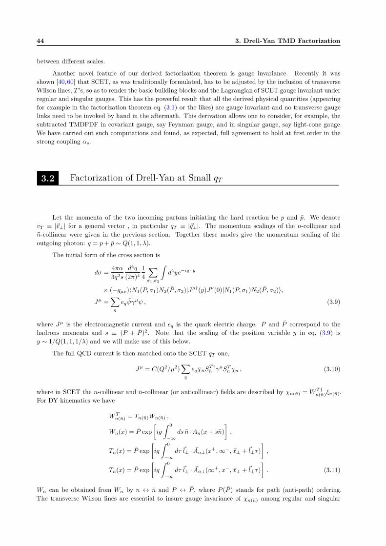
44 3. Drell-Yan TMD Factorization
between different scales.
Another novel feature of our derived factorization theorem is gauge invariance. Recently it was
shown [40,60] that SCET, as was traditionally formulated, has to be adjusted by the inclusion of transverse
Wilson lines, T ’s, so as to render the basic building blocks and the Lagrangian of SCET gauge invariant under
regular and singular gauges. This has the powerful result that all the derived physical quantities (appearing
for example in the factorization theorem eq. (3.1) or the likes) are gauge invariant and no transverse gauge
links need to be invoked by hand in the aftermath. This derivation allows one to consider, for example, the
subtracted TMDPDF in covariant gauge, say Feynman gauge, and in singular gauge, say light-cone gauge.
We have carried out such computations and found, as expected, full agreement to hold at first order in the
strong coupling αs.
3.2 Factorization of Drell-Yan at Small qT
Let the momenta of the two incoming partons initiating the hard reaction be p and p. We denote
vT ≡ |~v⊥| for a general vector , in particular qT ≡ |~q⊥|. The momentum scalings of the n-collinear and
n-collinear were given in the previous section. Together these modes give the momentum scaling of the
outgoing photon: q = p+ p ∼ Q(1, 1, λ).
The initial form of the cross section is
dσ =4πα
3q2s
d4q
(2π)4
1
4
∑
σ1,σ2
∫
d4ye−iq · y
× (−gµν)〈N1(P, σ1)N2(P , σ2)|Jµ†(y)Jν(0)|N1(P, σ1)N2(P , σ2)〉,Jµ =
∑
q
eqψγµψ , (3.9)
where Jµ is the electromagnetic current and eq is the quark electric charge. P and P correspond to the
hadrons momenta and s ≡ (P + P )2. Note that the scaling of the position variable y in eq. (3.9) is
y ∼ 1/Q(1, 1, 1/λ) and we will make use of this below.
The full QCD current is then matched onto the SCET-qT one,
Jµ = C(Q2/µ2)∑
q
eqχnST†n γµST
n χn , (3.10)
where in SCET the n-collinear and n-collinear (or anticollinear) fields are described by χn(n) = WT†n(n)ξn(n).
For DY kinematics we have
WTn(n) = Tn(n)Wn(n) ,
Wn(x) = P exp
[
ig
∫ 0
−∞
ds n ·An(x+ sn)
]
,
Tn(x) = P exp
[
ig
∫ 0
−∞
dτ ~l⊥ · ~An⊥(x+,∞−, ~x⊥ +~l⊥τ)
]
,
Tn(x) = P exp
[
ig
∫ 0
−∞
dτ ~l⊥ · ~An⊥(∞+, x−, ~x⊥ +~l⊥τ)
]
. (3.11)
Wn can be obtained from Wn by n ↔ n and P ↔ P , where P (P ) stands for path (anti-path) ordering.
The transverse Wilson lines are essential to insure gauge invariance of χn(n) among regular and singular
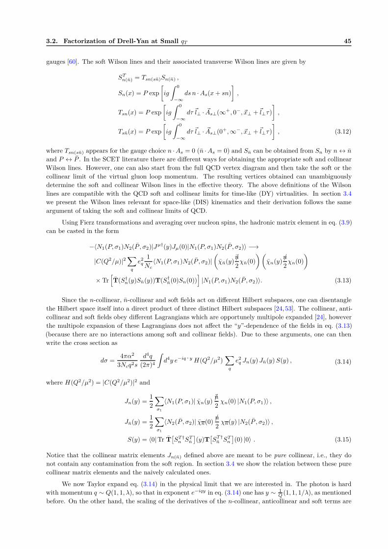
3.2. Factorization of Drell-Yan at Small qT 45
gauges [60]. The soft Wilson lines and their associated transverse Wilson lines are given by
STn(n) = Tsn(sn)Sn(n) ,
Sn(x) = P exp
[
ig
∫ 0
−∞
ds n ·As(x+ sn)
]
,
Tsn(x) = P exp
[
ig
∫ 0
−∞
dτ ~l⊥ · ~As⊥(∞+, 0−, ~x⊥ +~l⊥τ)
]
,
Tsn(x) = P exp
[
ig
∫ 0
−∞
dτ ~l⊥ · ~As⊥(0+,∞−, ~x⊥ +~l⊥τ)
]
, (3.12)
where Tsn(sn) appears for the gauge choice n ·As = 0 (n ·As = 0) and Sn can be obtained from Sn by n ↔ n
and P ↔ P . In the SCET literature there are different ways for obtaining the appropriate soft and collinear
Wilson lines. However, one can also start from the full QCD vertex diagram and then take the soft or the
collinear limit of the virtual gluon loop momentum. The resulting vertices obtained can unambiguously
determine the soft and collinear Wilson lines in the effective theory. The above definitions of the Wilson
lines are compatible with the QCD soft and collinear limits for time-like (DY) virtualities. In section 3.4
we present the Wilson lines relevant for space-like (DIS) kinematics and their derivation follows the same
argument of taking the soft and collinear limits of QCD.
Using Fierz transformations and averaging over nucleon spins, the hadronic matrix element in eq. (3.9)
can be casted in the form
−〈N1(P, σ1)N2(P , σ2)|Jµ†(y)Jµ(0)|N1(P, σ1)N2(P , σ2)〉 −→
|C(Q2/µ)|2∑
q
e2q
1
Nc〈N1(P, σ1)N2(P , σ2)|
(
χn(y)n/
2χn(0)
)(
χn(y)n/
2χn(0)
)
× Tr[
T(S†n(y)Sn(y))T(S†n(0)Sn(0))]
|N1(P, σ1)N2(P , σ2)〉. (3.13)
Since the n-collinear, n-collinear and soft fields act on different Hilbert subspaces, one can disentangle
the Hilbert space itself into a direct product of three distinct Hilbert subspaces [24, 53]. The collinear, anti-
collinear and soft fields obey different Lagrangians which are opportunely multipole expanded [24], however
the multipole expansion of these Lagrangians does not affect the “y”-dependence of the fields in eq. (3.13)
(because there are no interactions among soft and collinear fields). Due to these arguments, one can then
write the cross section as
dσ =4πα2
3Ncq2s
d4q
(2π)4
∫
d4y e−iq · y H(Q2/µ2)∑
q
e2q Jn(y)Jn(y)S(y) , (3.14)
where H(Q2/µ2) = |C(Q2/µ2)|2 and
Jn(y) =1
2
∑
σ1
〈N1(P, σ1)| χn(y)/n
2χn(0) |N1(P, σ1)〉 ,
Jn(y) =1
2
∑
σ1
〈N2(P , σ2)| χn(0)/n
2χn(y) |N2(P , σ2)〉 ,
S(y) = 〈0| Tr T[
ST†n ST
n
]
(y)T[
ST†n ST
n
]
(0) |0〉 . (3.15)
Notice that the collinear matrix elements Jn(n) defined above are meant to be pure collinear, i.e., they do
not contain any contamination from the soft region. In section 3.4 we show the relation between these pure
collinear matrix elements and the naively calculated ones.
We now Taylor expand eq. (3.14) in the physical limit that we are interested in. The photon is hard
with momentum q ∼ Q(1, 1, λ), so that in exponent e−iqy in eq. (3.14) one has y ∼ 1Q (1, 1, 1/λ), as mentioned
before. On the other hand, the scaling of the derivatives of the n-collinear, anticollinear and soft terms are
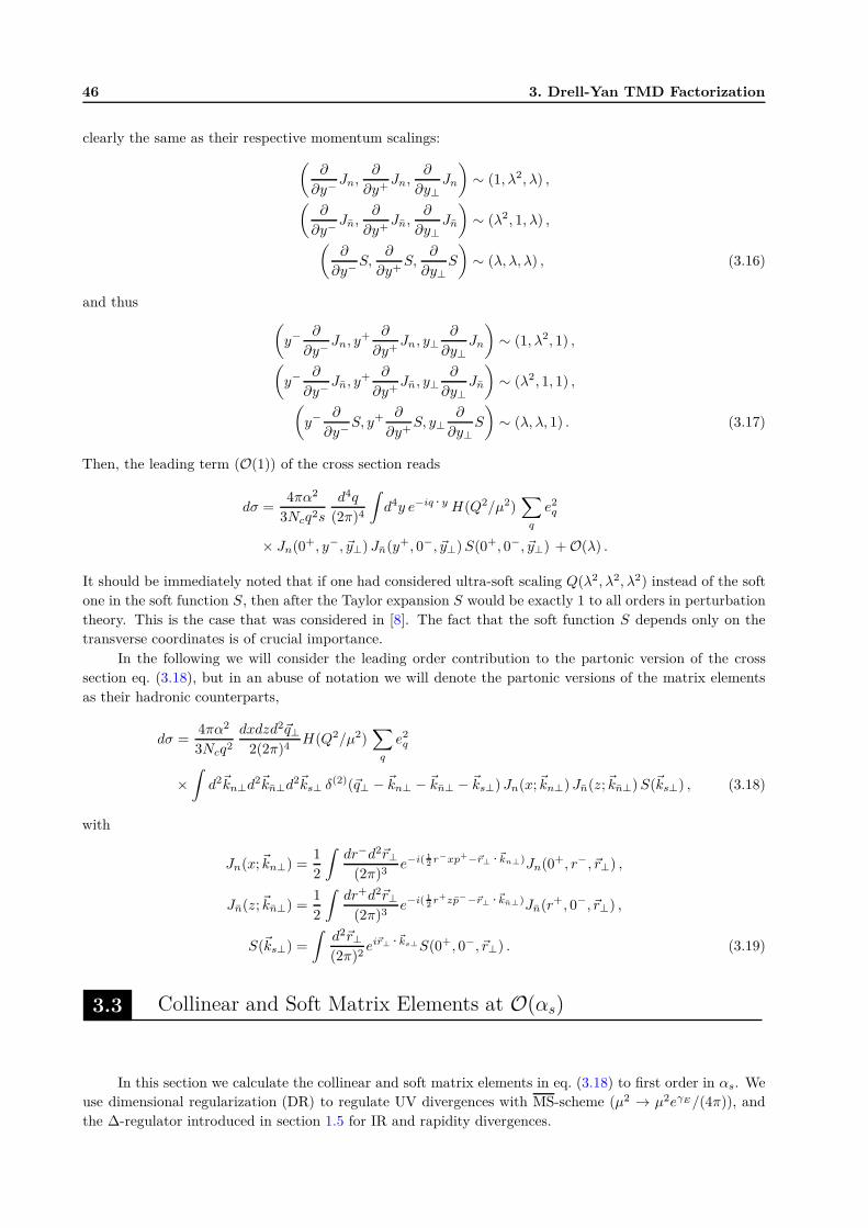
46 3. Drell-Yan TMD Factorization
clearly the same as their respective momentum scalings:
(
∂
∂y−Jn,
∂
∂y+Jn,
∂
∂y⊥Jn
)
∼ (1, λ2, λ) ,
(
∂
∂y−Jn,
∂
∂y+Jn,
∂
∂y⊥Jn
)
∼ (λ2, 1, λ) ,
(
∂
∂y−S,
∂
∂y+S,
∂
∂y⊥S
)
∼ (λ, λ, λ) , (3.16)
and thus(
y−∂
∂y−Jn, y
+ ∂
∂y+Jn, y⊥
∂
∂y⊥Jn
)
∼ (1, λ2, 1) ,
(
y−∂
∂y−Jn, y
+ ∂
∂y+Jn, y⊥
∂
∂y⊥Jn
)
∼ (λ2, 1, 1) ,
(
y−∂
∂y−S, y+ ∂
∂y+S, y⊥
∂
∂y⊥S
)
∼ (λ, λ, 1) . (3.17)
Then, the leading term (O(1)) of the cross section reads
dσ =4πα2
3Ncq2s
d4q
(2π)4
∫
d4y e−iq · y H(Q2/µ2)∑
q
e2q
× Jn(0+, y−, ~y⊥)Jn(y+, 0−, ~y⊥)S(0+, 0−, ~y⊥) + O(λ) .
It should be immediately noted that if one had considered ultra-soft scaling Q(λ2, λ2, λ2) instead of the soft
one in the soft function S, then after the Taylor expansion S would be exactly 1 to all orders in perturbation
theory. This is the case that was considered in [8]. The fact that the soft function S depends only on the
transverse coordinates is of crucial importance.
In the following we will consider the leading order contribution to the partonic version of the cross
section eq. (3.18), but in an abuse of notation we will denote the partonic versions of the matrix elements
as their hadronic counterparts,
dσ =4πα2
3Ncq2
dxdzd2~q⊥2(2π)4
H(Q2/µ2)∑
q
e2q
×∫
d2~kn⊥d2~kn⊥d
2~ks⊥ δ(2)(~q⊥ − ~kn⊥ − ~kn⊥ − ~ks⊥)Jn(x;~kn⊥)Jn(z;~kn⊥)S(~ks⊥) , (3.18)
with
Jn(x;~kn⊥) =1
2
∫
dr−d2~r⊥(2π)3
e−i( 12
r−xp+−~r⊥ ·~kn⊥)Jn(0+, r−, ~r⊥) ,
Jn(z;~kn⊥) =1
2
∫
dr+d2~r⊥(2π)3
e−i( 12
r+zp−−~r⊥ ·~kn⊥)Jn(r+, 0−, ~r⊥) ,
S(~ks⊥) =
∫
d2~r⊥(2π)2
ei~r⊥ ·~ks⊥S(0+, 0−, ~r⊥) . (3.19)
3.3 Collinear and Soft Matrix Elements at O(αs)
In this section we calculate the collinear and soft matrix elements in eq. (3.18) to first order in αs. We
use dimensional regularization (DR) to regulate UV divergences with MS-scheme (µ2 → µ2eγE/(4π)), and
the ∆-regulator introduced in section 1.5 for IR and rapidity divergences.
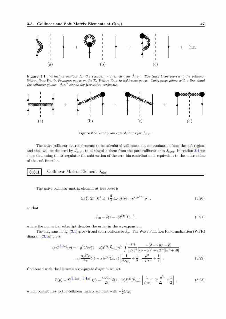
3.3. Collinear and Soft Matrix Elements at O(αs) 47
Figure 3.1: Virtual corrections for the collinear matrix element Jn(n). The black blobs represent the collinearWilson lines Wn in Feynman gauge or the Tn Wilson lines in light-cone gauge. Curly propagators with a line standfor collinear gluons. “h.c.” stands for Hermitian conjugate.
Figure 3.2: Real gluon contributions for Jn(n).
The naive collinear matrix elements to be calculated will contain a contamination from the soft region,
and thus will be denoted by Jn(n), to distinguish them from the pure collinear ones Jn(n). In section 3.4 we
show that using the ∆-regulator the subtraction of the zero-bin contribution is equivalent to the subtraction
of the soft function.
3.3.1 Collinear Matrix Element Jn(n)
The naive collinear matrix element at tree level is
〈p| ξn(ξ−, 0+, ξ⊥)n/
2ξn(0) |p〉 = ei 1
2p+ξ−
p+ , (3.20)
so that
Jn0 = δ(1 − x)δ(2)(~kn⊥) , (3.21)
where the numerical subscript denotes the order in the αs expansion.
The diagrams in fig. (3.1) give virtual contributions to Jn. The Wave Function Renormalization (WFR)
diagram (3.1a) gives
ip/Σ(3.1a)(p) = −g2CF δ(1 − x)δ(2)(~kn⊥)µ2ǫ
∫
ddk
(2π)d
−(d− 2)(p/− k/)
[(p− k)2 + i∆−][k2 + i0]
= ip/αsCF
2πδ(1 − x)δ(2)(~kn⊥)
[
1
2εUV+
1
2ln
µ2
−i∆− +1
4
]
. (3.22)
Combined with the Hermitian conjugate diagram we get
Σ(p) = Σ(3.1a)+(3.1a)∗
(p) =αsCF
2πδ(1 − x)δ(2)(~kn⊥)
[
1
εUV+ ln
µ2
∆−+
1
2
]
, (3.23)
which contributes to the collinear matrix element with − 12 Σ(p).
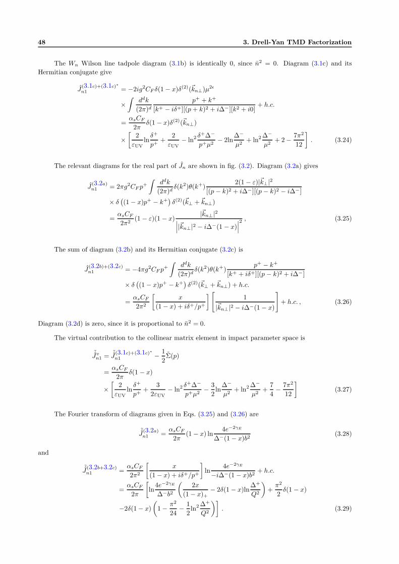
48 3. Drell-Yan TMD Factorization
The Wn Wilson line tadpole diagram (3.1b) is identically 0, since n2 = 0. Diagram (3.1c) and its
Hermitian conjugate give
J(3.1c)+(3.1c)∗
n1 = −2ig2CF δ(1 − x)δ(2)(~kn⊥)µ2ǫ
×∫
ddk
(2π)d
p+ + k+
[k+ − iδ+][(p+ k)2 + i∆−][k2 + i0]+ h.c.
=αsCF
2πδ(1 − x)δ(2)(~kn⊥)
×[
2
εUVlnδ+
p++
2
εUV− ln2 δ
+∆−
p+µ2− 2ln
∆−
µ2+ ln2 ∆−
µ2+ 2 − 7π2
12
]
. (3.24)
The relevant diagrams for the real part of Jn are shown in fig. (3.2). Diagram (3.2a) gives
J(3.2a)n1 = 2πg2CF p
+
∫
ddk
(2π)dδ(k2)θ(k+)
2(1 − ε)|~k⊥|2[(p− k)2 + i∆−][(p− k)2 − i∆−]
× δ(
(1 − x)p+ − k+)
δ(2)(~k⊥ + ~kn⊥)
=αsCF
2π2(1 − ε)(1 − x)
|~kn⊥|2∣
∣
∣|~kn⊥|2 − i∆−(1 − x)
∣
∣
∣
2 , (3.25)
The sum of diagram (3.2b) and its Hermitian conjugate (3.2c) is
J(3.2b)+(3.2c)n1 = −4πg2CF p
+
∫
ddk
(2π)dδ(k2)θ(k+)
p+ − k+
[k+ + iδ+][(p− k)2 + i∆−]
× δ(
(1 − x)p+ − k+)
δ(2)(~k⊥ + ~kn⊥) + h.c.
=αsCF
2π2
[
x
(1 − x) + iδ+/p+
]
[
1
|~kn⊥|2 − i∆−(1 − x)
]
+ h.c. , (3.26)
Diagram (3.2d) is zero, since it is proportional to n2 = 0.
The virtual contribution to the collinear matrix element in impact parameter space is
˜Jv
n1 =˜J
(3.1c)+(3.1c)∗
n1 − 1
2Σ(p)
=αsCF
2πδ(1 − x)
×[
2
εUVlnδ+
p++
3
2εUV− ln2 δ
+∆−
p+µ2− 3
2ln
∆−
µ2+ ln2 ∆−
µ2+
7
4− 7π2
12
]
(3.27)
The Fourier transform of diagrams given in Eqs. (3.25) and (3.26) are
˜J
(3.2a)n1 =
αsCF
2π(1 − x) ln
4e−2γE
∆−(1 − x)b2(3.28)
and
˜J
(3.2b+3.2c)n1 =
αsCF
2π2
[
x
(1 − x) + iδ+/p+
]
ln4e−2γE
−i∆−(1 − x)b2+ h.c.
=αsCF
2π
[
ln4e−2γE
∆−b2
(
2x
(1 − x)+− 2δ(1 − x)ln
∆+
Q2
)
+π2
2δ(1 − x)
−2δ(1 − x)
(
1 − π2
24− 1
2ln2 ∆+
Q2
)]
. (3.29)
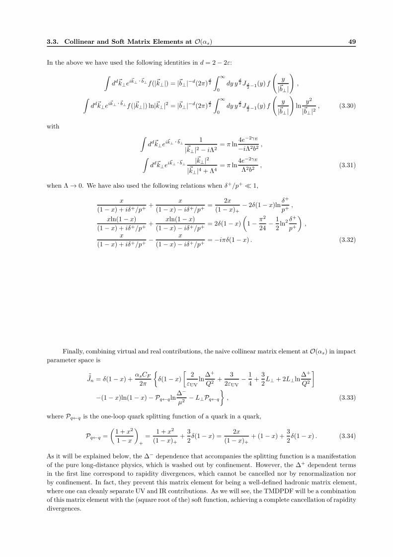
3.3. Collinear and Soft Matrix Elements at O(αs) 49
In the above we have used the following identities in d = 2 − 2ε:
∫
dd~k⊥ei~k⊥ ·~b⊥f(|~k⊥|) = |~b⊥|−d(2π)
d2
∫ ∞
0
dy yd2 J d
2−1(y) f
(
y
|~b⊥|
)
,
∫
dd~k⊥ei~k⊥ ·~b⊥f(|~k⊥|) ln|~k⊥|2 = |~b⊥|−d(2π)
d2
∫ ∞
0
dy yd2 J d
2−1(y) f
(
y
|~b⊥|
)
lny2
|~b⊥|2, (3.30)
with
∫
dd~k⊥ei~k⊥ ·~b⊥
1
|~k⊥|2 − iΛ2= π ln
4e−2γE
−iΛ2b2,
∫
dd~k⊥ei~k⊥ ·~b⊥
|~k⊥|2
|~k⊥|4 + Λ4= π ln
4e−2γE
Λ2b2, (3.31)
when Λ → 0. We have also used the following relations when δ+/p+ ≪ 1,
x
(1 − x) + iδ+/p++
x
(1 − x) − iδ+/p+=
2x
(1 − x)+− 2δ(1 − x)ln
δ+
p+,
xln(1 − x)
(1 − x) + iδ+/p++
xln(1 − x)
(1 − x) − iδ+/p+= 2δ(1 − x)
(
1 − π2
24− 1
2ln2 δ
+
p+
)
,
x
(1 − x) + iδ+/p+− x
(1 − x) − iδ+/p+= −iπδ(1 − x) . (3.32)
Finally, combining virtual and real contributions, the naive collinear matrix element at O(αs) in impact
parameter space is
˜Jn = δ(1 − x) +
αsCF
2π
{
δ(1 − x)
[
2
εUVln
∆+
Q2+
3
2εUV− 1
4+
3
2L⊥ + 2L⊥ln
∆+
Q2
]
−(1 − x)ln(1 − x) − Pq←qln∆−
µ2− L⊥Pq←q
}
, (3.33)
where Pq←q is the one-loop quark splitting function of a quark in a quark,
Pq←q =
(
1 + x2
1 − x
)
+
=1 + x2
(1 − x)++
3
2δ(1 − x) =
2x
(1 − x)++ (1 − x) +
3
2δ(1 − x) . (3.34)
As it will be explained below, the ∆− dependence that accompanies the splitting function is a manifestation
of the pure long-distance physics, which is washed out by confinement. However, the ∆+ dependent terms
in the first line correspond to rapidity divergences, which cannot be cancelled nor by renormalization nor
by confinement. In fact, they prevent this matrix element for being a well-defined hadronic matrix element,
where one can cleanly separate UV and IR contributions. As we will see, the TMDPDF will be a combination
of this matrix element with the (square root of the) soft function, achieving a complete cancellation of rapidity
divergences.
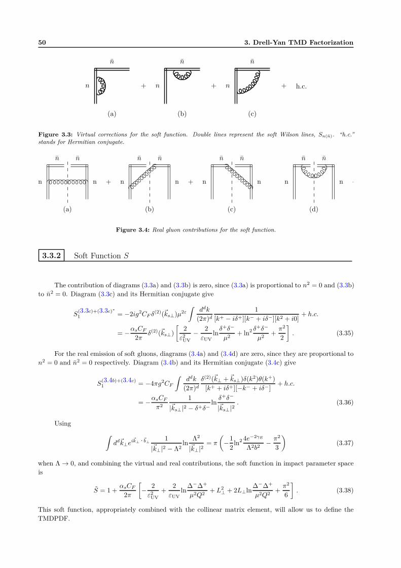
50 3. Drell-Yan TMD Factorization
Figure 3.3: Virtual corrections for the soft function. Double lines represent the soft Wilson lines, Sn(n). “h.c.”stands for Hermitian conjugate.
Figure 3.4: Real gluon contributions for the soft function.
3.3.2 Soft Function S
The contribution of diagrams (3.3a) and (3.3b) is zero, since (3.3a) is proportional to n2 = 0 and (3.3b)
to n2 = 0. Diagram (3.3c) and its Hermitian conjugate give
S(3.3c)+(3.3c)∗
1 = −2ig2CF δ(2)(~ks⊥)µ2ε
∫
ddk
(2π)d
1
[k+ − iδ+][k− + iδ−][k2 + i0]+ h.c.
= −αsCF
2πδ(2)(~ks⊥)
[
2
ε2UV
− 2
εUVlnδ+δ−
µ2+ ln2 δ
+δ−
µ2+π2
2
]
. (3.35)
For the real emission of soft gluons, diagrams (3.4a) and (3.4d) are zero, since they are proportional to
n2 = 0 and n2 = 0 respectively. Diagram (3.4b) and its Hermitian conjugate (3.4c) give
S(3.4b)+(3.4c)1 = −4πg2CF
∫
ddk
(2π)d
δ(2)(~k⊥ + ~ks⊥)δ(k2)θ(k+)
[k+ + iδ+][−k− + iδ−]+ h.c.
= −αsCF
π2
1
|~ks⊥|2 − δ+δ−lnδ+δ−
|~ks⊥|2. (3.36)
Using
∫
dd~k⊥ei~k⊥ ·~b⊥
1
|~k⊥|2 − Λ2ln
Λ2
|~k⊥|2= π
(
−1
2ln2 4e−2γE
Λ2b2− π2
3
)
(3.37)
when Λ → 0, and combining the virtual and real contributions, the soft function in impact parameter space
is
S = 1 +αsCF
2π
[
− 2
ε2UV
+2
εUVln
∆−∆+
µ2Q2+ L2
⊥ + 2L⊥ln∆−∆+
µ2Q2+π2
6
]
. (3.38)
This soft function, appropriately combined with the collinear matrix element, will allow us to define the
TMDPDF.
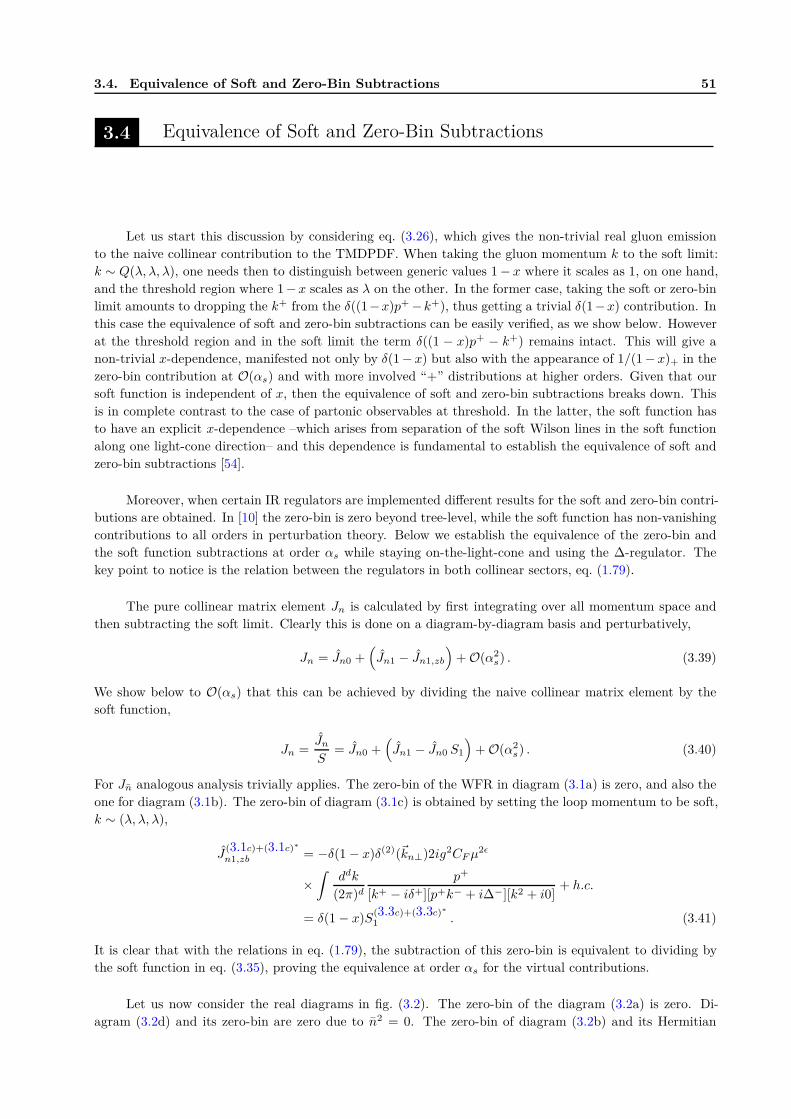
3.4. Equivalence of Soft and Zero-Bin Subtractions 51
3.4 Equivalence of Soft and Zero-Bin Subtractions
Let us start this discussion by considering eq. (3.26), which gives the non-trivial real gluon emission
to the naive collinear contribution to the TMDPDF. When taking the gluon momentum k to the soft limit:
k ∼ Q(λ, λ, λ), one needs then to distinguish between generic values 1 − x where it scales as 1, on one hand,
and the threshold region where 1 −x scales as λ on the other. In the former case, taking the soft or zero-bin
limit amounts to dropping the k+ from the δ((1−x)p+ −k+), thus getting a trivial δ(1−x) contribution. In
this case the equivalence of soft and zero-bin subtractions can be easily verified, as we show below. However
at the threshold region and in the soft limit the term δ((1 − x)p+ − k+) remains intact. This will give a
non-trivial x-dependence, manifested not only by δ(1 − x) but also with the appearance of 1/(1 − x)+ in the
zero-bin contribution at O(αs) and with more involved “+” distributions at higher orders. Given that our
soft function is independent of x, then the equivalence of soft and zero-bin subtractions breaks down. This
is in complete contrast to the case of partonic observables at threshold. In the latter, the soft function has
to have an explicit x-dependence –which arises from separation of the soft Wilson lines in the soft function
along one light-cone direction– and this dependence is fundamental to establish the equivalence of soft and
zero-bin subtractions [54].
Moreover, when certain IR regulators are implemented different results for the soft and zero-bin contri-
butions are obtained. In [10] the zero-bin is zero beyond tree-level, while the soft function has non-vanishing
contributions to all orders in perturbation theory. Below we establish the equivalence of the zero-bin and
the soft function subtractions at order αs while staying on-the-light-cone and using the ∆-regulator. The
key point to notice is the relation between the regulators in both collinear sectors, eq. (1.79).
The pure collinear matrix element Jn is calculated by first integrating over all momentum space and
then subtracting the soft limit. Clearly this is done on a diagram-by-diagram basis and perturbatively,
Jn = Jn0 +(
Jn1 − Jn1,zb
)
+ O(α2s) . (3.39)
We show below to O(αs) that this can be achieved by dividing the naive collinear matrix element by the
soft function,
Jn =Jn
S= Jn0 +
(
Jn1 − Jn0 S1
)
+ O(α2s) . (3.40)
For Jn analogous analysis trivially applies. The zero-bin of the WFR in diagram (3.1a) is zero, and also the
one for diagram (3.1b). The zero-bin of diagram (3.1c) is obtained by setting the loop momentum to be soft,
k ∼ (λ, λ, λ),
J(3.1c)+(3.1c)∗
n1,zb = −δ(1 − x)δ(2)(~kn⊥)2ig2CFµ2ǫ
×∫
ddk
(2π)d
p+
[k+ − iδ+][p+k− + i∆−][k2 + i0]+ h.c.
= δ(1 − x)S(3.3c)+(3.3c)∗
1 . (3.41)
It is clear that with the relations in eq. (1.79), the subtraction of this zero-bin is equivalent to dividing by
the soft function in eq. (3.35), proving the equivalence at order αs for the virtual contributions.
Let us now consider the real diagrams in fig. (3.2). The zero-bin of the diagram (3.2a) is zero. Di-
agram (3.2d) and its zero-bin are zero due to n2 = 0. The zero-bin of diagram (3.2b) and its Hermitian
52 3. Drell-Yan TMD Factorization
conjugate (3.2c) is
J(3.2b)+(3.2c)n1,zb = −4πg2CF δ(1 − x)
∫
d4k
(2π)4
p+δ(k2)θ(k+)δ(2)(k⊥ − kn⊥)
[−k+ + iδ+][p+k− + i∆−]+ h.c.
= δ(1 − x)S(3.4b)+(3.4c)1 , (3.42)
which is equivalent to divide by the soft function diagram (3.4b) and its Hermitian conjugate (3.4c), given
in eq. (3.36), thanks again to the relation in eq. (1.79).
In conclusion, we have proved to first order in αs that, using the ∆-regulator, subtracting the zero-bin
is equivalent to divide the naive collinear matrix element by the soft function, which leads us to the following
relation between the pure collinear Jn(n) and naive collinear Jn(n) matrix elements,
Jn(0+, r−, ~r⊥) =Jn(0+, r−, ~r⊥)
S(0+, 0−, ~r⊥), Jn(r+, 0−, ~r⊥) =
Jn(r+, 0−, ~r⊥)
S(0+, 0−, ~r⊥), (3.43)
where
Jn(0+, r−, ~r⊥) = 〈p|[
ξnWTn
]
(0+, y−, ~y⊥)n/
2
[
WT†n ξn
]
(0) |p〉|zb included ,
Jn(r+, 0−, ~r⊥) = 〈p|[
ξnWTn
]
(0)n/
2
[
WT†n ξn
]
(y+, 0−, ~y⊥) |p〉|zb included . (3.44)
Thus, using the results in the previous section, the pure collinear matrix element at O(αs) is
Jn1 =αsCF
2π
{
δ(1 − x)
[
2
ε2UV
− 2
εUVln
∆−
µ2+
3
2εUV− 1
4− 2π2
12− L2
⊥ +3
2L⊥
−2L⊥ln∆−
µ2
]
− (1 − x)ln(1 − x) − Pq←qln∆−
µ2− L⊥Pq←q
}
. (3.45)
3.5 Extraction of the Hard Coefficient H at O(αs)
Once we have calculated the collinear and soft matrix elements, let us now establish the factorization
theorem given in eq. (3.18) by calculating the hard matching coefficient H(Q2/µ2) to first order in αs. The
hard part for the qT -dependent DY cross section is the same as the one for inclusive DY. As mentioned
before, this matching coefficient at the higher scale Q is obtained by matching the virtual contribution of
the full QCD cross section onto the virtual one of the imaginary part of the product of two effective theory
currents. This echoes the “subtraction method” in perturbative QCD.
We start by rewriting eq. (3.18) as
dσ =4πα2
3Ncq2
dxdzd2~q⊥2(2π)4
∑
q
e2qM(x, z; ~q⊥, Q) ,
M(x, z; ~q⊥, Q) = H(Q2/µ2)[
δ(1 − x)δ(1 − z)δ(2)(~q⊥)
+(
δ(1 − z)Jn1(x; ~q⊥, Q, µ) + δ(1 − x)Jn1(z; ~q⊥, Q, µ)
+δ(1 − x)δ(1 − z)S1(~q⊥))]
+O(α2s) , (3.46)
where M is the so-called hadronic tensor, which can be also written in terms of the naive collinear matrix
3.5. Extraction of the Hard Coefficient H at O(αs) 53
elements,
M(x, z; ~q⊥, Q) = H(Q2/µ2)[
δ(1 − x)δ(1 − z)δ(2)(~q⊥)
+(
δ(1 − z) Jn1(x; ~q⊥, Q, µ) + δ(1 − x) Jn1(z; ~q⊥, Q, µ)
−δ(1 − x)δ(1 − z)S1(~q⊥))]
+O(α2s) . (3.47)
In QCD, the virtual part of M with ∆-regulator is
MvQCD = δ(1 − x)δ(1 − z)δ(2)(~q⊥)
{
1 +αsCF
2π
[
−2ln2 ∆
Q2− 3ln
∆
Q2− 9
2+π2
2
]}
. (3.48)
The above result can be simply obtained by considering the one-loop correction to the vertex diagram for
qq → γ∗, with the inclusion of the WFR diagram while using the fermion propagators in eq. (1.77) with
∆± = ∆. The explicit calculation can be found in section 1.5.2.
Collecting the results in section 3.3, we can write the virtual part of the naive collinear and soft matrix
elements with ∆± = ∆,
Jvn1 =
αsCF
2πδ(1 − x)δ(2)(~kn⊥)
×[
2
εUVln
∆
Q2+
3
2εUV− ln2 ∆2
Q2µ2− 3
2ln
∆
µ2+ ln2 ∆
µ2+
7
4− 7π2
12
]
Jvn1 =
αsCF
2πδ(1 − z)δ(2)(~kn⊥)
×[
2
εUVln
∆
Q2+
3
2εUV− ln2 ∆2
Q2µ2− 3
2ln
∆
µ2+ ln2 ∆
µ2+
7
4− 7π2
12
]
Sv1 =
αsCF
2πδ(2)(~ks⊥)
[
− 2
ε2UV
+2
εUVln
∆2
Q2µ2− ln2 ∆2
Q2µ2− π2
2
]
. (3.49)
Thus, inserting the results above in eq. (3.47), the total virtual part of the hadronic tensor M in the effective
theory is
MvSCET = H(Q2/µ2)δ(1 − x)δ(1 − z)δ(2)(~q⊥)
{
1 +αsCF
2π
[
2
ε2UV
+1
εUV
(
3 + 2lnµ2
Q2
)
− 2ln2 ∆
Q2− 3ln
∆
Q2+ 3ln
µ2
Q2+ ln2 µ
2
Q2+
7
2− 2π2
3
]}
, (3.50)
where the UV divergences are canceled by the standard renormalization process. We notice that the IR
contributions in Eqs. (3.48, 3.50) are the same, thus the matching coefficient between QCD and the effective
theory at scale Q is:
H(Q2/µ2) = 1 +αsCF
2π
[
−3lnµ2
Q2− ln2 µ
2
Q2− 8 +
7π2
6
]
. (3.51)
The above result was first derived in [61,62]. We can also obtain the AD of the hard matching coefficient at
O(αs),
γH1 =dlnH
dlnµ= −αsCF
2π
[
6 + 4lnµ2
Q2
]
. (3.52)
So we conclude that the factorization theorem in eq. (3.18) is satisfied to first order in αs. The IR
divergences of full QCD are recovered in the effective theory calculation, eq. (3.50). Notice that the rapidity
divergences are cancelled in the combination of the collinear and soft matrix elements, as they should since
we do not have rapidity divergences in full QCD, and thus can be easily identified. And finally, the matching
54 3. Drell-Yan TMD Factorization
coefficient at the higher scale depends only on the hard scale Q2, as it should be.
3.6 Preliminary Definition of the TMDPDF
The problem with the factorization formula in eq. (3.18) is that in the O(αs) calculation of Jn(n) and
S there are still rapidity divergences, which complicate both the renormalization procedure and the non-
perturbative interpretation of such quantities. As we have shown in the previous section, these divergences
cancel in the combination of the collinear and soft matrix elements, as they should, because in full QCD there
are no rapidity divergences. In other words, while using the ∆-regulator, the only ∆ dependence that remains
after combining collinear and soft matrix elements is pure IR, a manifestation in the partonic calculation of
the long-distance physics that is washed out by confinement. In conclusion, each matrix element individually
is ill-defined and cannot be considered as a physical quantity.
However, when considering the following combinations
Fn(x;~kn⊥) =1
2
∫
dr−d2~r⊥(2π)3
e−i( 12
r−xp+−~r⊥ ·~kn⊥)Jn(0+, r−, ~r⊥)√
S(0+, 0−, ~r⊥) ,
Fn(z;~kn⊥) =1
2
∫
dr+d2~r⊥(2π)3
e−i( 12
r+zp−−~r⊥ ·~kn⊥)Jn(r+, 0−, ~r⊥)√
S(0+, 0−, ~r⊥) , (3.53)
it turns out that those quantities are free from such rapidity divergences. This is shown explicitly to hold
to O(αs) in the next section. In the next chapter we will see that this preliminary definition of TMDPDF
is based on some assumption over the IR regulator, and thus needs to be generalized. For the moment, we
will show that it fulfills our requirements for a well-defined quantity, i.e., it is free from rapidity divergences.
Given the equivalence of the zero-bin and soft subtraction with the implementation of the ∆-regulator,
we can write the TMDPDFs in the following way as well,
Fn(x;~kn⊥) =1
2
∫
dr−d2~r⊥(2π)3
e−i( 12
r−xp+−~r⊥ ·~kn⊥) Jn(0+, r−, ~r⊥)√
S(0+, 0−, ~r⊥),
Fn(z;~kn⊥) =1
2
∫
dr+d2~r⊥(2π)3
e−i( 12
r+zp−−~r⊥ ·~kn⊥) Jn(r+, 0−, ~r⊥)√
S(0+, 0−, ~r⊥), (3.54)
where the square root of the soft function is subtracted from the naive collinear matrix element. Notice that
this particular definition of the TMDPDF only applies when the subtraction of the zero-bin and the soft
function are equivalent.
Thus it is compelling to re-cast the factorization theorem in eq. (3.18) in the following form,
dσ =4πα2
3Ncq2
dxdzd2~q⊥2(2π)4
H(Q2/µ2)∑
q
e2q
×∫
d2~kn⊥d2~kn⊥ δ
(2)(~q⊥ − ~kn⊥ − ~kn⊥)Fn(x;~kn⊥, µ)Fn(z;~kn⊥, µ) . (3.55)
The TMDPDFs Fn(n) are defined in general in eq. (3.53), but in the following we take the result in eq. (3.54),
which applies for our particular kinematical regime (perturbative qT and away from threshold) and for the
set of IR regulators implemented below (∆-regulator).
Expanding eq. (3.53) to first order in αs one finds
Fn(x;~kn⊥, Q, µ) =1
2
∫
dξ−d2~ξ⊥(2π)3
e−i( 12
ξ−xp+−~ξ⊥ ·~kn⊥)
[
Jn0 +
(
Jn1 +1
2Jn0S1
)]
+ O(α2s) , (3.56)
3.6. Preliminary Definition of the TMDPDF 55
where the numerical subscripts denote the order in the αs expansion. Using the tree-level result for Jn in
section 3.3, the expansion of Fn up to order αs is
Fn(x;~kn⊥, Q, µ) = δ(1 − x)δ(2)(~kn⊥)
+
[
1
2
∫
dξ−d2~ξ⊥(2π)3
e−i( 12
ξ−xp+−~ξ⊥ ·~kn⊥)Jn1 +1
2δ(1 − x)
∫
d2~ξ⊥(2π)2
ei~ξ⊥ ·~kn⊥S1
]
, (3.57)
which in IPS reads
Fn(x;~kn⊥, Q, µ) = Jn
√
S
= δ(1 − x) + Jn1 +1
2δ(1 − x)S1 + O(α2
s) . (3.58)
Collecting the results in section 3.3, the TMDPDF in IPS at O(αs) is
Fn = δ(1 − x) +αsCF
2π
{
δ(1 − x)
[
1
ε2UV
+3
2εUV− 1
εUVlnQ2
µ2
−1
2L2⊥ +
3
2L⊥ − L⊥ln
Q2
µ2− π2
12
]
+ (1 − x) − L⊥Pq←q
−Pq←qln∆
µ2− 1
4δ(1 − x) − (1 − x)[1 + ln(1 − x)]
}
. (3.59)
where we have set ∆+ = ∆− = ∆. As mentioned earlier, individual contributions to Fn(n) contain rapidity
divergences, however Fn(n) itself is free from them, and the only ∆ dependence that appears in the equation
above encodes pure IR physics.
Finally, we calculate the anomalous dimension of the TMDPDF to O(αs), for which one needs to
consider only its virtual contributions since, as we have seen in section 3.3, all real contributions are UV-
finite. From eq. (3.59) the counterterm for the n-collinear TMDPDF is
Zn = 1 − αsCF
2π
[
1
ε2UV
+1
εUV
(
3
2+ ln
µ2
Q2
)]
, (3.60)
and the corresponding anomalous dimension is
γn =dlnZn
dlnµ=
1
Z
∂Z
∂lnµ+
1
Z
∂Z
∂αs
∂αs
∂lnµ=
1
Zn
∂Zn
∂lnµ+
1
Zn
∂Zn
∂αs(−2εαs + O(α2
s))
γn1 =αsCF
2π
[
3 + 2lnµ2
Q2
]
. (3.61)
For the n-collinear sector we have, analogously, Zn, from which we get
γn1 =dlnZn
dlnµ=αsCF
2π
[
3 + 2lnµ2
Q2
]
. (3.62)
In section 3.7.1.1 we give the AD of the TMDPDF at second and third orders in αs.
3.6.1 Anomalous Dimension in Dimensional Regularization
It is possible to calculate the anomalous dimension of the TMDPDF using pure DR as in [54]. At one-
loop, we need only to consider the virtual contributions given in diagrams (3.1a), (3.1c) and (3.3c). All the
rest vanish identically due to light-like Wilson lines. For diagram (3.1a) (without its Hermitian conjugate)
56 3. Drell-Yan TMD Factorization
we have
J(3.1a)n1 =
αsCF
4πδ(1 − x)δ(2)(~kn⊥)
(
1
εUV− 1
εIR
)
, (3.63)
and for diagram (3.1c),
J(3.1c)n1 =
αsCF
4πδ(1 − x)δ(2)(~kn⊥)
×(
µ2
−κ(p+)2
)ε [1
εIR
(
2
εUV− 2
εIR
)
+
(
2
εUV− 2
εIR
)]
. (3.64)
Notice that in this regularization scheme the energy scale inside the logs is fixed noting that p+ is the only
relevant scale in the virtual part of the TMDPDF. Thus the scale inside the logs is equal to −κ(p+)2 where
κ = Q2/(p+)2 and it is required to remove the dimensional ambiguity in integrals of the form:∫∞
0dt t−1−ε.
The soft function, diagram (3.3c), gives
S(3.3c)1 = −αsCF
2πδ(2)(~kn⊥)
(
µ2
−κ(p+)2
)ε
2
[
1
εUV− 1
εIR
]2
. (3.65)
Taking into account the Hermitian conjugate diagrams, the total virtual contribution to the TMDPDF is
F vn1 =
αsCF
2πδ(1 − x)δ(2)(~kn⊥)
1
ε2UV
−2ln(
κ(p+)2
µ2
)
− 3
2εUV− 1
ε2IR
+2ln(
κ(p+)2
µ2
)
− 3
2εIR
. (3.66)
From the result for F vn1, one can easily identify the counter-term Zn needed to cancel the UV divergences
and one gets
γn1 =αsCF
2π
[
3 + 2lnµ2
κ(p+)2
]
=αsCF
2π
[
3 + 2lnµ2
Q2
]
, (3.67)
which agrees with eq. (3.61).
In eq. (3.66) we again notice that there are no mixed UV and IR divergences. It should be noted that
if one had subtracted the complete soft function from the collinear part (and not the square root of it) then
there would be mixed UV and IR poles and those mixed poles would not cancel even after including the
contribution from real gluon emission. This would definitely prevent such quantity from being an acceptable
definition of TMDPDF.
3.7 Refactorization: from TMDPDF to PDF
When qT ≫ ΛQCD, the factorization theorem in eq. (3.18) is not the final form yet and the TMDPDFs
still have to be refactorized. In the effective theory approach this corresponds to a second step matching of
SCET-qT , that describes the physics at the intermediate scale qT ≫ ΛQCD, onto SCET-II, that captures
the non-perturbative physics at the hadronic scale ΛQCD.
The refactorization of the TMDPDF is essential since the collinear and soft contribution that enter
in the definition of Fn(n) live at the intermediate scale qT , consistent with their construction in SCET-qT .
Since qT is perturbative, its conjugate coordinate, the impact parameter b, is small enough to perform an
OPE in the impact parameter space. Moreover in this space the IR structure becomes manifest with the
appearance of IR poles in dimensional regularization. Obviously, the first term in the OPE would be just the
standard Feynman PDF, and the Wilson coefficient would be the term that sums all the large logs between
ΛQCD and qT (see refs. [4, 5, 50] and more recently using SCET refs. [6, 8, 10, 42]). Then, given the following
3.7. Refactorization: from TMDPDF to PDF 57
OPE (and the analogous for n),
Fn(x;~b⊥, µ) =
∫ 1
x
dx′
x′Cn
( x
x′;~b⊥, µ
)
fn(x′;µ) + O(b2Λ2QCD) , (3.68)
where
Fn(x;~b⊥, µ) =
∫
d2~kn⊥ ei~kn⊥ ·~b⊥Fn(x;~kn⊥, µ) (3.69)
and
fn(x;µ) =1
2
∫
dy−
2πe−i 1
2y−xp+ 〈p| χn(0+, y−,~0⊥)
n/
2χ†n(0+, 0−,~0⊥) |p〉 |zb included , (3.70)
the factorization theorem takes the form
dσ =4πα2
3Ncq2
dxdzd2~q⊥2(2π)4
∑
q
e2q
∫
d2~b⊥(2π)2
e−i~q⊥ ·~b⊥
∫ 1
x
dx′
x′
∫ 1
z
dz′
z′
×H(Q2/µ2) Cn
( x
x′;~b⊥, Q, µ
)
Cn
( z
z′;~b⊥, Q, µ
)
fn(x′;µ) fn(z′;µ) . (3.71)
In this effort and for simplicity of presentation we will not consider the contribution coming from a
gluon splitting into two quarks. This contribution is certainly vital for the final result of the DY cross-section.
Here however we are mainly interested in studying the TMDPDF of a quark in a quark. Henceforth we will
refer to this quantity simply as the “TMDPDF” and it can be easily checked that all the results below are
not affected by this omission.
The above result is one of the main results of this chapter and it holds to all orders in perturbation
theory. It is worthy to notice the separation of scales: the hard matching coefficient lives at scale Q, the
matching coefficients at the intermediate scale live at 1/b ∼ qT , and finally the PDFs live at the hadronic
scale ΛQCD.
As we show below in section 3.7.1, Cn(n) have a subtle Q2-dependence which at first sight might spoil
the scale factorization, however this dependence can be extracted and exponentiated, thus putting it under
control.
The complete TMDPDF to first order in αs was given in eq. (3.59), and its renormalized result is
Fn1 = δ(1 − x) +αsCF
2π
{
δ(1 − x)
[
−1
2L2⊥ +
3
2L⊥ − L⊥ln
Q2
µ2− π2
12
]
+ (1 − x)
−L⊥Pq←q − Pq←qln∆
µ2− 1
4δ(1 − x) − (1 − x)[1 + ln(1 − x)]
}
. (3.72)
We will match this result onto the integrated PDF, which we cal calculate below. The virtual diagrams for
the PDF are the same as for the collinear matrix element that enters into the definition of the TMDPDF,
fig. (3.1). From eqs. (3.22) and (3.24) we get
Σ(p) = Σ(3.1a)+(3.1a)∗
(p) =αsCF
2πδ(1 − x)δ(2)(~kn⊥)
[
1
εUV+ ln
µ2
∆−+
1
2
]
, (3.73)
which contributes to the PDF with − 12 Σ(p), and
f (3.1c)+(3.1c)∗
n =αsCF
2πδ(1 − x)
[
2
εUVln
∆+
Q2+
2
εUV− ln2 ∆+
Q2− 2ln
∆+
Q2ln
∆−
µ2
−2ln∆−
µ2+ 2 − 7π2
12
]
. (3.74)
58 3. Drell-Yan TMD Factorization
The real diagrams are the same as in fig. (3.2), from which we get
f (3.2a)n = 2πg2CF p
+
∫
ddk
(2π)d
2(1 − ε)|~k⊥|2δ(k2)θ(k+)δ ((1 − x)p+ − k+)
[(p− k)2 + i∆−][(p− k)2 − i∆−]
=αsCF
2π(1 − x)
[
1
εUV+ ln
µ2
∆−− 1 − ln(1 − x)
]
, (3.75)
and
f (3.2b)+(3.2c)n = −4πg2CF p
+µ2ε
∫
ddk
(2π)dδ(k2)θ(k+)
p+ − k+
[k+ + iδ+][(p− k)2 + i∆−]
× δ(
(1 − x)p+ − k+)
+ h.c.
=αsCF
2π
[(
1
εUV+ ln
µ2
∆−
)(
2x
(1 − x)+− 2δ(1 − x)ln
∆+
Q2
)
−2δ(1 − x)
(
1 − π2
24− 1
2ln2 ∆+
Q2
)
+π2
2δ(1 − x)
]
, (3.76)
where we have used MS-scheme (µ2 → µ2eγE/(4π)) and the following relations when δ+/p+ ≪ 1,
x
(1 − x) + iδ+/p++
x
(1 − x) − iδ+/p+=
2x
(1 − x)+− 2δ(1 − x)ln
δ+
p+,
x(1 − x)−ε
(1 − x) + iδ+/p++
x(1 − x)−ε
(1 − x) − iδ+/p+= 2
[
x
(1 − x)+− δ(1 − x)ln
δ+
p+
−εδ(1 − x)
(
1 − π2
24− 1
2ln2 δ
+
p+
)]
+ O(ε2) ,
x
(1 − x) + iδ+/p+− x
(1 − x) − iδ+/p+= −iπδ(1 − x) . (3.77)
Combining the virtual and real contributions we get the PDF to first order in αs,
fn(x;µ) = δ(1 − x) +αsCF
2π
[
Pq←q
(
1
εUV− ln
∆−
µ2
)
−1
4δ(1 − x) − (1 − x) [1 + ln(1 − x)]
]
. (3.78)
Finally, setting ∆± = ∆, we can extract the matching coefficient of the TMDPDF given in eq. (3.72)
onto the PDF given in the equation above, obtaining
Cn = δ(1 − x) +αsCF
2π
[
− LT Pq←q + (1 − x)
− δ(1 − x)
(
1
2L2
T − 3
2LT + LT ln
Q2
µ2+π2
12
)
]
. (3.79)
At this stage it is worth noticing the appearance of ln(Q2/µ2) at the matching coefficient. From the
above result, we can see that by a proper choice of the scale µ = µI ≡ (2e−γE/b), we eliminate this logarithm
since LT (µI) = 0. However at this order in perturbation theory this cancelation is accidental and it does
not persist at higher orders. In the following section we discuss the appearance of ln(Q2/µ2) at an arbitrary
order in perturbation theory and how to handle them.
3.7. Refactorization: from TMDPDF to PDF 59
3.7.1 Q2-Dependence and Resummation
The matching coefficient Cn is expected to live at the intermediate scale qT ∼ 1/b. However the
appearance of ln(Q2/µ2) in Cn1, and higher powers of it in higher orders in perturbation theory, might
indicate otherwise. Notice, for example, that the logarithms in eq. (3.79) cannot be combined into a simple
logarithm, unlike the case of threshold region in inclusive Drell-Yan or DIS [39,61]. In the threshold region the
matching coefficient at the intermediate scale µI is a function of only one logarithm, ln(µ2I/µ
2). Nonetheless,
from general arguments concerning the ∆-regulator we can extract and exponentiate this Q2-dependence in
the TMDPDF itself, thus putting it under control to all orders in perturbation theory.
Working in pure DR and setting all scaleless integrals to zero, only real diagrams contribute to Fn.
Then, we can express the logarithm of the TMDPDF in impact parameter space as
lnFn = ln˜Jn − 1
2lnS , (3.80)
where
ln˜Jn = Rn
(
x;αs, LT , lnδ+
p+= ln
∆
Q2
)
,
lnS = Rs
(
αs, LT , lnδ+δ−
µ2= ln
∆2
Q2µ2
)
, (3.81)
and we have set ∆± = ∆. The need for ∆-regulator to regulate rapidity divergences in individual Feynman
diagrams of˜Jn and S introduces the logarithmic dependencies shown in eq. (3.84). Due to dimensional
arguments and Lorentz invariance, those are the only possible combinations that can appear.
Since the PDF is zero in pure DR and the matching coefficient between the TMDPDF and the PDF
does not depend on the IR regulator, we have
d
dln∆lnFn = 0 , (3.82)
which implies that Rn and Rs must be linear in their last arguments. Thus we can write
lnFn = lnFQ/n −D(αs, LT )
(
lnQ2
µ2+ LT
)
, (3.83)
where we have introduced LT just to cancel the µ2-dependence in the coefficient of D which simplifies the
RG equations of the TMDPDF. The function lnFQ/n is independent of Q2 and all the Q2-dependence appears
explicitly only in the ln(Q2/µ2). Hence, we can extract all the Q2-dependence from the TMDPDF and
exponentiate it, putting it under control.
We believe that the linearity in ln(Q2/µ2) can be extracted without relying on a particular scheme of
regularization, but based on general arguments concerning the rapidity divergences. As we have shown in
section 3.6 to first order in αs, the TMDPDF is free from rapidity divergences, since all the ∆-dependence
that remains exactly matches the IR contribution of full QCD. Then, although our ∆-regulator does not
differentiate the origin of the divergences that it regulates, i.e., it encodes both the IR (soft and collinear)
and rapidity divergences, actually one could use another regulator that makes this distinction manifest. For
instance the ν-regulator introduced in [10].
Now, if we denote by ν the parameter that regulates only the rapidity divergences (and using a different
ones for the IR), then we believe that, based on the O(αs) calculation, the functional dependence of ln˜Jn
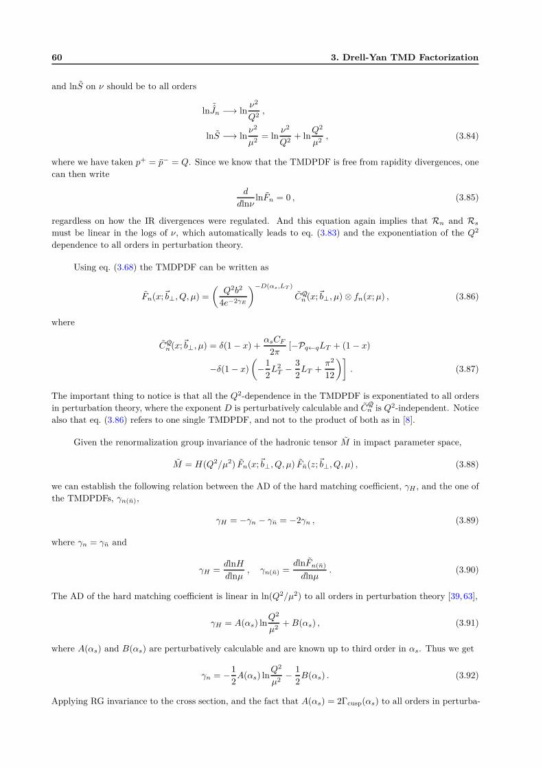
60 3. Drell-Yan TMD Factorization
and lnS on ν should be to all orders
ln˜Jn −→ ln
ν2
Q2,
lnS −→ lnν2
µ2= ln
ν2
Q2+ ln
Q2
µ2, (3.84)
where we have taken p+ = p− = Q. Since we know that the TMDPDF is free from rapidity divergences, one
can then write
d
dlnνlnFn = 0 , (3.85)
regardless on how the IR divergences were regulated. And this equation again implies that Rn and Rs
must be linear in the logs of ν, which automatically leads to eq. (3.83) and the exponentiation of the Q2
dependence to all orders in perturbation theory.
Using eq. (3.68) the TMDPDF can be written as
Fn(x;~b⊥, Q, µ) =
(
Q2b2
4e−2γE
)−D(αs,LT )
CQ/n (x;~b⊥, µ) ⊗ fn(x;µ) , (3.86)
where
CQ/n (x;~b⊥, µ) = δ(1 − x) +
αsCF
2π[−Pq←qLT + (1 − x)
−δ(1 − x)
(
−1
2L2
T − 3
2LT +
π2
12
)]
. (3.87)
The important thing to notice is that all the Q2-dependence in the TMDPDF is exponentiated to all orders
in perturbation theory, where the exponent D is perturbatively calculable and CQ/n is Q2-independent. Notice
also that eq. (3.86) refers to one single TMDPDF, and not to the product of both as in [8].
Given the renormalization group invariance of the hadronic tensor M in impact parameter space,
M = H(Q2/µ2) Fn(x;~b⊥, Q, µ) Fn(z;~b⊥, Q, µ) , (3.88)
we can establish the following relation between the AD of the hard matching coefficient, γH , and the one of
the TMDPDFs, γn(n),
γH = −γn − γn = −2γn , (3.89)
where γn = γn and
γH =dlnH
dlnµ, γn(n) =
dlnFn(n)
dlnµ. (3.90)
The AD of the hard matching coefficient is linear in ln(Q2/µ2) to all orders in perturbation theory [39, 63],
γH = A(αs) lnQ2
µ2+B(αs) , (3.91)
where A(αs) and B(αs) are perturbatively calculable and are known up to third order in αs. Thus we get
γn = −1
2A(αs) ln
Q2
µ2− 1
2B(αs) . (3.92)
Applying RG invariance to the cross section, and the fact that A(αs) = 2Γcusp(αs) to all orders in perturba-
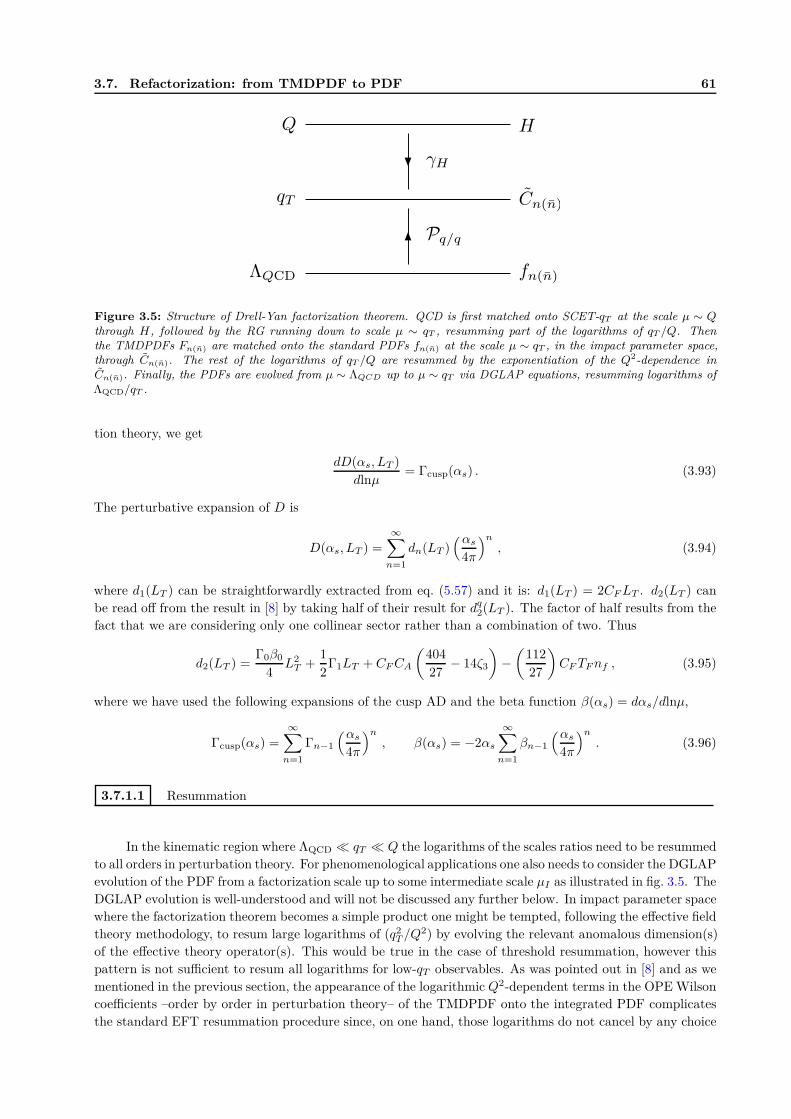
3.7. Refactorization: from TMDPDF to PDF 61
Figure 3.5: Structure of Drell-Yan factorization theorem. QCD is first matched onto SCET-qT at the scale µ ∼ Qthrough H, followed by the RG running down to scale µ ∼ qT , resumming part of the logarithms of qT /Q. Thenthe TMDPDFs Fn(n) are matched onto the standard PDFs fn(n) at the scale µ ∼ qT , in the impact parameter space,through Cn(n). The rest of the logarithms of qT /Q are resummed by the exponentiation of the Q2-dependence inCn(n). Finally, the PDFs are evolved from µ ∼ ΛQCD up to µ ∼ qT via DGLAP equations, resumming logarithms ofΛQCD/qT .
tion theory, we get
dD(αs, LT )
dlnµ= Γcusp(αs) . (3.93)
The perturbative expansion of D is
D(αs, LT ) =
∞∑
n=1
dn(LT )(αs
4π
)n
, (3.94)
where d1(LT ) can be straightforwardly extracted from eq. (5.57) and it is: d1(LT ) = 2CFLT . d2(LT ) can
be read off from the result in [8] by taking half of their result for dq2(LT ). The factor of half results from the
fact that we are considering only one collinear sector rather than a combination of two. Thus
d2(LT ) =Γ0β0
4L2
T +1
2Γ1LT + CFCA
(
404
27− 14ζ3
)
−(
112
27
)
CFTFnf , (3.95)
where we have used the following expansions of the cusp AD and the beta function β(αs) = dαs/dlnµ,
Γcusp(αs) =
∞∑
n=1
Γn−1
(αs
4π
)n
, β(αs) = −2αs
∞∑
n=1
βn−1
(αs
4π
)n
. (3.96)
3.7.1.1 Resummation
In the kinematic region where ΛQCD ≪ qT ≪ Q the logarithms of the scales ratios need to be resummed
to all orders in perturbation theory. For phenomenological applications one also needs to consider the DGLAP
evolution of the PDF from a factorization scale up to some intermediate scale µI as illustrated in fig. 3.5. The
DGLAP evolution is well-understood and will not be discussed any further below. In impact parameter space
where the factorization theorem becomes a simple product one might be tempted, following the effective field
theory methodology, to resum large logarithms of (q2T /Q
2) by evolving the relevant anomalous dimension(s)
of the effective theory operator(s). This would be true in the case of threshold resummation, however this
pattern is not sufficient to resum all logarithms for low-qT observables. As was pointed out in [8] and as we
mentioned in the previous section, the appearance of the logarithmic Q2-dependent terms in the OPE Wilson
coefficients –order by order in perturbation theory– of the TMDPDF onto the integrated PDF complicates
the standard EFT resummation procedure since, on one hand, those logarithms do not cancel by any choice
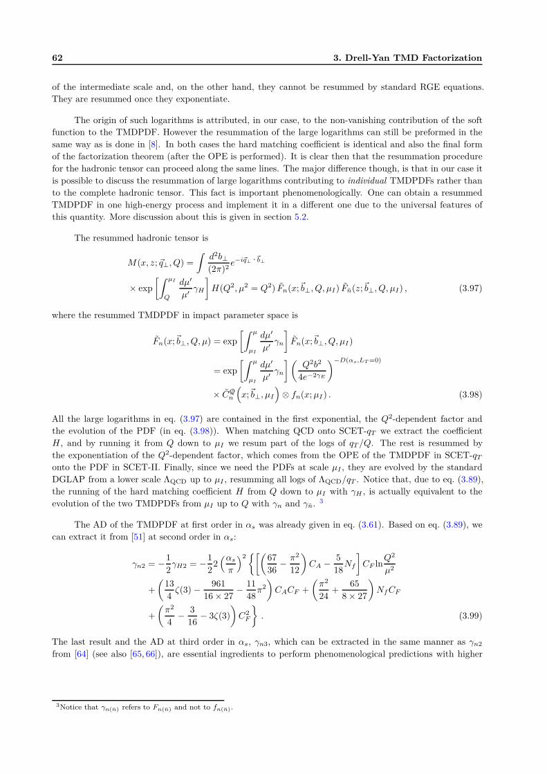
62 3. Drell-Yan TMD Factorization
of the intermediate scale and, on the other hand, they cannot be resummed by standard RGE equations.
They are resummed once they exponentiate.
The origin of such logarithms is attributed, in our case, to the non-vanishing contribution of the soft
function to the TMDPDF. However the resummation of the large logarithms can still be preformed in the
same way as is done in [8]. In both cases the hard matching coefficient is identical and also the final form
of the factorization theorem (after the OPE is performed). It is clear then that the resummation procedure
for the hadronic tensor can proceed along the same lines. The major difference though, is that in our case it
is possible to discuss the resummation of large logarithms contributing to individual TMDPDFs rather than
to the complete hadronic tensor. This fact is important phenomenologically. One can obtain a resummed
TMDPDF in one high-energy process and implement it in a different one due to the universal features of
this quantity. More discussion about this is given in section 5.2.
The resummed hadronic tensor is
M(x, z; ~q⊥, Q) =
∫
d2b⊥(2π)2
e−i~q⊥ ·~b⊥
× exp
[∫ µI
Q
dµ′
µ′γH
]
H(Q2, µ2 = Q2) Fn(x;~b⊥, Q, µI) Fn(z;~b⊥, Q, µI) , (3.97)
where the resummed TMDPDF in impact parameter space is
Fn(x;~b⊥, Q, µ) = exp
[∫ µ
µI
dµ′
µ′γn
]
Fn(x;~b⊥, Q, µI)
= exp
[∫ µ
µI
dµ′
µ′γn
](
Q2b2
4e−2γE
)−D(αs,LT =0)
× CQ/n
(
x;~b⊥, µI
)
⊗ fn(x;µI) . (3.98)
All the large logarithms in eq. (3.97) are contained in the first exponential, the Q2-dependent factor and
the evolution of the PDF (in eq. (3.98)). When matching QCD onto SCET-qT we extract the coefficient
H , and by running it from Q down to µI we resum part of the logs of qT /Q. The rest is resummed by
the exponentiation of the Q2-dependent factor, which comes from the OPE of the TMDPDF in SCET-qT
onto the PDF in SCET-II. Finally, since we need the PDFs at scale µI , they are evolved by the standard
DGLAP from a lower scale ΛQCD up to µI , resumming all logs of ΛQCD/qT . Notice that, due to eq. (3.89),
the running of the hard matching coefficient H from Q down to µI with γH , is actually equivalent to the
evolution of the two TMDPDFs from µI up to Q with γn and γn. 3
The AD of the TMDPDF at first order in αs was already given in eq. (3.61). Based on eq. (3.89), we
can extract it from [51] at second order in αs:
γn2 = −1
2γH2 = −1
22(αs
π
)2{[(
67
36− π2
12
)
CA − 5
18Nf
]
CF lnQ2
µ2
+
(
13
4ζ(3) − 961
16 × 27− 11
48π2
)
CACF +
(
π2
24+
65
8 × 27
)
NfCF
+
(
π2
4− 3
16− 3ζ(3)
)
C2F
}
. (3.99)
The last result and the AD at third order in αs, γn3, which can be extracted in the same manner as γn2
from [64] (see also [65, 66]), are essential ingredients to perform phenomenological predictions with higher
3Notice that γn(n) refers to Fn(n) and not to fn(n).
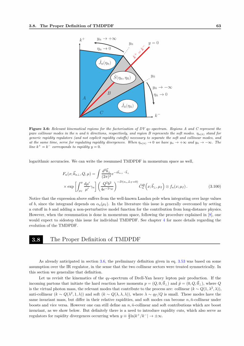
3.8. The Proper Definition of TMDPDF 63
k+ =
k−
yn → +∞
yn → −∞
k+
k−
A
C
Jn(ηn)
Jn(ηn)
B
S(ηn, ηn)
ηn → 0
ηn → 0
y = 0yn
yn
Figure 3.6: Relevant kinematical regions for the factorization of DY qT -spectrum. Regions A and C represent thepure collinear modes in the n and n directions, respectively, and region B represents the soft modes. ηn(n) stand forgeneric rapidity regulators (and not explicit rapidity cutoffs) necessary to separate the soft and collinear modes, andat the same time, serve for regulating rapidity divergences. When ηn(n) → 0 we have yn → +∞ and yn → −∞. Theline k+ = k− corresponds to rapidity y = 0.
logarithmic accuracies. We can write the resummed TMDPDF in momentum space as well,
Fn(x;~kn⊥, Q, µ) =
∫
d2~b⊥(2π)2
e−i~kn⊥ ·~b⊥
× exp
[∫ µ
µI
dµ′
µ′γn
](
Q2b2
4e−2γE
)−D(αs,LT =0)
CQ/n
(
x;~b⊥, µI
)
⊗ fn(x;µI) . (3.100)
Notice that the expression above suffers from the well-known Landau pole when integrating over large values
of b, since the integrand depends on αs(µI). In the literature this issue is generally overcomed by setting
a cutoff in b and adding a non-perturbative model function for the contribution from long-distance physics.
However, when the resummation is done in momentum space, following the procedure explained in [8], one
would expect to sidestep this issue for individual TMDPDF. See chapter 4 for more details regarding the
evolution of the TMDPDF.
3.8 The Proper Definition of TMDPDF
As already anticipated in section 3.6, the preliminary definition given in eq. 3.53 was based on some
assumption over the IR regulator, in the sense that the two collinear sectors were treated symmetrically. In
this section we generalize that definition.
Let us revisit the kinematics of the qT -spectrum of Drell-Yan heavy lepton pair production. If the
incoming partons that initiate the hard reaction have momenta p = (Q, 0,~0⊥) and p = (0, Q,~0⊥), where Q
is the virtual photon mass, the relevant modes that contribute to the process are: collinear (k ∼ Q(1, λ2, λ)),
anti-collinear (k ∼ Q(λ2, 1, λ)) and soft (k ∼ Q(λ, λ, λ)), where λ ∼ qT /Q is small. These modes have the
same invariant mass, but differ in their relative rapidities, and soft modes can become n, n-collinear under
boosts and vice versa. However one can still define an n, n-collinear and soft contributions which are boost
invariant, as we show below. But definitely there is a need to introduce rapidity cuts, which also serve as
regulators for rapidity divergences occurring when y ≡ 12 ln|k+/k−| → ±∞.
64 3. Drell-Yan TMD Factorization
In fig. 3.6 ηn(n) are generic rapidity regulators that separate soft modes from the n, n-collinear ones.
They also serve as regulators for the rapidity divergences that appear in the collinear and soft matrix elements.
Those regulators should disappear when one combines all matrix elements within the factorization theorem,
since in full QCD there are no rapidity divergences.
In terms of these generic rapidity regulators ηn(n), the hadronic tensor for the qT -dependent DY spec-
trum can be split in impact parameter space as
M = H(Q2) Jn(ηn) S(ηn, ηn) Jn(ηn) , (3.101)
where we show explicitly just the rapidity regulator dependence. As already explained in section 3.2, S is
the relevant soft function and Jn(n) stand for pure (anti-)collinear contributions, which are calculated first by
integrating over all momentum space and then subtracting the “zero-bin” contribution, i.e., the soft limit of
the collinear integrands [34] (see also [38]). Generally speaking, this should be done on a diagram-by-diagram
basis. At operator level one can identify those soft contaminations with the soft function itself [53–55],
however this equivalence might get spoiled for certain regulators 4. Thus at the level of the factorization
theorem itself, one should refrain from subtracting the soft function (since this would be based on a regulator-
dependent arguments) and formulate the relevant theorem in terms of pure collinear matrix elements and
soft functions as in eq. (3.101).
Previously we have implemented the ∆-regulator to regulate IR and rapidity divergences, and as shown
in eq. (1.78), the consistency between full QCD and its collinear and soft limits leads to a relation between
δ± and ∆± through the large components of the parton momenta. In particular, the soft function which,
at operator level, does not know about δ’s (or ∆’s), will have a dependence on p+ and p− because in
perturbation theory those regulators will be invoked. By considering the denominators of the propagators in
eq. (1.77), it is clear that one should treat the ∆± as boost invariant quantities, i.e., they transform as the
product p+p−, while δ+ transforms as k+ or p+ (or 1/p−) and δ− transforms as k− or p− (or 1/p+). Those
observations will be used below.
Using the ∆-regulator one can relate ηn with ∆− and ηn with ∆+ only in the terms where the ∆’s
regularize rapidity divergences, but not in the terms with IR divergences (which are also regularized by ∆±).
When all matrix elements are combined in eq. (3.101) there will remain a ∆-dependence which is exactly
the genuine IR divergences of perturbative QCD. This remaining ∆-dependence is not worrisome since,
hadronically, it disappears by confinement, i.e., due to non-perturbative QCD contributions in exactly the
same manner as the collinear divergence of the partonic integrated PDF signals the onset of non-perturbative
(long distance) contribution. The distinction between rapidity divergences and the IR ones will become more
clear in the following section, where we show explicit results for the collinear and soft matrix elements and
comment on them.
In eq. (3.53) the soft function appearing in eq. (3.101) was split identically between the two collinear
sectors and the TMDPDFs were defined as
F pren = J (0)
n (∆−)
√
S
(
∆−
p+,
∆+
p−
)
∣
∣
∣
∣
∣
∆+=∆−
,
F pren = J
(0)n (∆+)
√
S
(
∆−
p+,
∆+
p−
)
∣
∣
∣
∣
∣
∆+=∆−
, (3.102)
where “pre” stands for “preliminary” and the ∆-regulator was used to regularize all the IR and the rapidity
4Explicit examples can be found in eq. (64) of [34], and also in [10] where the zero-bin contributions vanish beyond tree-levelwhile the soft function does not.

3.8. The Proper Definition of TMDPDF 65
divergences. The O(αs) result for the TMDPDF, before renormalization, was
F pren1 =
αsCF
2π
{
δ(1 − xn)
[
1
ε2UV
+3
2εUV− 1
εUVlnQ2∆−
µ2∆+
−1
2L2⊥ +
3
2L⊥ − L⊥ln
Q2∆−
µ2∆+− π2
12
]
+ (1 − xn) − L⊥Pq←q
−Pq←qln∆−
µ2− 1
4δ(1 − xn) − (1 − xn)[1 + ln(1 − xn)]
}
. (3.103)
where ∆+ = ∆−, as indicated in eq. (3.102). The new definition given below will be a generalization of this
one in the sense that no assumption will be made on the values of ∆±, although it reduces to the one in
eq. (3.102) for ∆+ = ∆−.
It is important to emphasize that in principle two disentangled collinear sectors should be treated
independently, thus it is crucial to examine what happens when we relax the condition ∆+ = ∆− and
consider the most general case where ∆+ 6= ∆−.
The first line in eq. (3.103) contains a rapidity divergence (mixed UV-IR term). The second line is
what would be the matching (or Wilson) coefficient of the TMDPDF onto the integrated PDF after an OPE
is carried out (see section 3.7), but it also contains an unacceptable dependence on the ∆-regulator, i.e., an
un-cancelled RD. As is well-known, Wilson coefficients should be free from any non-ultraviolet regulators,
either IR or RD. The last line is simply the integrated PDF (see section 3.7). In the next section we comment
on the origin of the Q2-dependence appearing above.
If we combine eq. (3.103) with the analogous result for F pren1 (where we just interchange ∆+ ↔ ∆− and
xn ↔ xn) the rapidity divergences cancel and the hard part H in M = H F pren F pre
n depends just on Q2/µ2,
as it should. However it is clear that only with the choice ∆+ = ∆− the rapidity divergences cancel in each
TMDPDF independently, both the mixed UV-IR divergence in the first line and the rapidity divergence in
the Wilson coefficient in the second line. It is important to notice that the limit
lim∆+→0∆−→0
ln∆−
∆+, (3.104)
has to be taken in order to get a well-defined physical quantity. Apart from the ∆−-dependence in the last
line of eq. (3.103), which is the manifestation of the genuine long-distance QCD effects and is washed out by
confinement, all the remaining ln(∆−
∆+ ) in the first two lines should cancel in that limit. But clearly this is not
the case. The independent behavior of ∆+ and ∆−, which is part of the implementation of the ∆-regulator
(reminiscent from taking the full QCD propagators with ∆± into the soft and collinear limits) renders that
limit as ill-defined since it could either be finite or ±∞. From the above it is thus clear that in order to avoid
any ad-hoc prescription for the regulators (∆+ = ∆−) a new definition of the TMDPDF should be adopted.
The new definition should nonetheless reduce to the one discussed previously when ∆+ = ∆−. Finally we
point out that the discussion of the equivalence between JCC and EIS approaches in [67] is valid only when
the limit in eq. (3.104) is finite. In this section we generalize the arguments in [67] to the general case where
there is no relation between ∆+ and ∆− and lim∆±→0 |ln(∆−/∆+)| = ∞.
Although our presentation so far was done in terms of the ∆-regulator, the results to be presented
below can be immediately generalized to other regulators as well. If one had used off-shellnesses [68], or the
ν-regulator as in [10], then our proposed TMDPDF would have the same features as with the ∆-regulator.
This has been checked explicitly. We will show next that by splitting the soft function in two “pieces” (and
not taking naively its square root), which will turn out to be a fundamental property of it that holds to all
orders in perturbation theory, and by combining them with the collinear matrix elements, we will be able to
properly define the TMDPDF and cancel rapidity divergences. But first, let us examine the nature of the
divergences in the soft function.
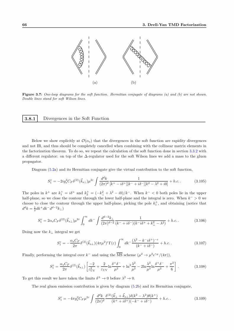
66 3. Drell-Yan TMD Factorization
(a) (b)
Figure 3.7: One-loop diagrams for the soft function. Hermitian conjugate of diagrams (a) and (b) are not shown.Double lines stand for soft Wilson lines.
3.8.1 Divergences in the Soft Function
Below we show explicitly at O(αs) that the divergences in the soft function are rapidity divergences
and not IR, and thus should be completely cancelled when combining with the collinear matrix elements in
the factorization theorem. To do so, we repeat the calculation of the soft function done in section 3.3.2 with
a different regulator: on top of the ∆-regulator used for the soft Wilson lines we add a mass to the gluon
propagator.
Diagram (5.2a) and its Hermitian conjugate give the virtual contribution to the soft function,
Sv1 = −2ig2
sCF δ(2)(~ks⊥)µ2ε
∫
ddk
(2π)d
1
[k+ − iδ+][k− + iδ−][k2 − λ2 + i0]+ h.c. . (3.105)
The poles in k+ are k+1 = iδ+ and k+
2 = (−k2⊥ + λ2 − i0)/k−. When k− < 0 both poles lie in the upper
half-plane, so we close the contour through the lower half-plane and the integral is zero. When k− > 0 we
choose to close the contour through the upper half-plane, picking the pole k+1 , and obtaining (notice that
ddk = 12dk
+dk−dd−2k⊥)
Sv1 = 2αsCF δ
(2)(~ks⊥)µ2ε
∫ ∞
0
dk−∫
dd−2k⊥(2π)d−2
1
(k− + iδ−)(k−iδ+ + k2⊥ − λ2)
+ h.c. . (3.106)
Doing now the k⊥ integral we get
Sv1 = −αsCF
2πδ(2)(~ks⊥)(4πµ2)εΓ(ε)
∫ ∞
0
dk−(λ2 − k−iδ+)−ε
(k− + iδ−)+ h.c. . (3.107)
Finally, performing the integral over k− and using the MS scheme (µ2 → µ2eγE/(4π)),
Sv1 =
αsCF
2πδ(2)(~ks⊥)
[ −2
ε2UV
+2
εUVlnδ+δ−
µ2+ ln2 λ
2
µ2− 2ln
λ2
µ2lnδ+δ−
µ2+π2
6
]
. (3.108)
To get this result we have taken the limits δ± → 0 before λ2 → 0.
The real gluon emission contribution is given by diagram (5.2b) and its Hermitian conjugate,
Sr1 = −4πg2
sCFµ2ε
∫
ddk
(2π)d
δ(2)(~k⊥ + ~ks⊥)δ(k2 − λ2)θ(k+)
(k+ + iδ+)(−k− + iδ−)+ h.c. . (3.109)
3.8. The Proper Definition of TMDPDF 67
Performing the integral over k− and k⊥ we get
Sr1 = −αsCF
2π
∫ ∞
0
dk+ 1
(k+ + iδ+)(k2s⊥ − λ2 + iδ−k+)
+ h.c.
= −αsCF
2π
1
|~ks⊥|2 + λ2ln
δ+δ−
|~ks⊥|2 + λ2. (3.110)
Using the results above, in impact parameter space we have for the virtual contribution
Sv1 =
αsCF
2π
[ −2
ε2UV
+2
εUVlnδ+δ−
µ2+ ln2 λ
2
µ2− 2ln
λ2
µ2lnδ+δ−
µ2+π2
6
]
, (3.111)
while for the real it is
Sr1 =
αsCF
2π
[
L2⊥ + 2L⊥ln
δ+δ−
µ2+ 2ln
λ2
µ2lnδ+δ−
µ2− ln2 λ
2
µ2
]
. (3.112)
To perform the Fourier transforms, we have used eq. (3.30) and
∫
dd~k⊥ei~k⊥ ·~b⊥
1
|~k⊥|2 + λ2= π ln
4e−2γE
λ2b2,
∫
dd~k⊥ei~k⊥ ·~b⊥
ln(
|~k⊥|2 + λ2)
(
|~k⊥|2 + λ2) = −πK0(bλ) ln
b2
4e−2γEλ2, (3.113)
that can be obtained by setting d = 2 right from the start because there are no UV divergences, and the IR
ones are regulated by λ2. We have also used the following expansion for the Bessel function
K0(bλ) =1
2ln
4e−2γE
b2λ2+ O
(
(bλ)2)
. (3.114)
Finally, combining virtual and real contributions in IPS, we obtain the soft function at O(αs),
S1 =αsCF
2π
[ −2
ε2UV
+2
εUVlnδ+δ−
µ2+ L2
⊥ + 2L⊥lnδ+δ−
µ2+π2
6
]
. (3.115)
Thus we see that all the dependence on λ2 cancels and there is just the δ± which regularizes only rapidity
divergences, inherent to the introduction of (soft) Wilson lines in the soft function. As mentioned before,
those rapidity divergences will cancel the ones in the pure collinear matrix elements and the only remaining
divergence in each TMDPDF will be just the collinear IR divergence.
3.8.2 Splitting the Soft Function
In the kinematical region where Q ≫ qT ≫ ΛQCD one can perform an operator product expansion
(OPE) of the result in eq. (3.101) onto the integrated PDFs where the hadronic tensor can be expressed as 5
M = H(Q2/µ2) C(xn, xn;L⊥, Q2/µ2)fn(xn; ∆−/µ2) fn(xn; ∆+/µ2) . (3.116)
The functions H and C are the two perturbatively calculable matching coefficients obtained after a two-step
matching at the scales Q and qT, respectively. Those coefficients are independent of any non-ultraviolet
regulators. In particular, using the ∆-regulator, they are independent of the ∆±.
5C(xn, xn; L⊥, Q2/µ2) = CQ/n (xn; L⊥) C
Q/n (xn; L⊥)
(
Q2
µ2
)−2D(αs(µ),L⊥(µ))
, consistent with eq. (3.86) and its analogous for
the anti-collinear TMDPDF.
68 3. Drell-Yan TMD Factorization
Since the integrated PDFs, fn(n), contain just the n, n-IR collinear divergences then each one of them
can be written in general as
lnfn = Rf1(xn, αs) + Rf2(xn, αs)ln∆−
µ2,
lnfn = Rf1(xn, αs) + Rf2(xn, αs)ln∆+
µ2, (3.117)
where Rf1 and Rf2 are some functions of αs(µ) and xn(n). The fact that lnfn has only a single ln∆−
µ2 (or
single IR pole in pure dimensional regularization) to all orders in perturbation theory is a well-known fact.
It has been shown [63] (see also [39]) that the anomalous dimension of the PDF in Mellin moment space has
a single logarithm lnN to all orders in perturbation theory. This single logarithm results from a single UV
pole in lnfn. For a massless matrix element such as the PDF, the single UV pole will always be accompanied
by a single IR pole in dimensional regularization, or a single ln ∆−
µ2 if one uses the ∆-regulator for the IR
divergences.
On the other hand we can express the hadronic tensor M in terms of matrix elements, as in eq. (3.101).
To separate the modes in rapidity we notice that each one of the pure collinear matrix elements does not have
any information about the other collinear sector. This is exactly due to the fact that the soft contamination
in the naively calculated collinear contribution has been subtracted out. By its definition, it is clear that
the soft function depends on both sectors, which is manifested through the dependence on both ∆’s. Given
this, and using boost invariance and dimensional analysis we can write
lnJ (0)n = Rn
(
xn, αs, L⊥, ln∆−
µ2
)
,
lnJ(0)n = Rn
(
xn, αs, L⊥, ln∆+
µ2
)
,
lnS = Rs
(
αs, L⊥, ln∆−∆+
Q2µ2
)
, (3.118)
where R(n,n,s) stand for generic functions.
Now, given that all the IR divergences of QCD are absorbed into two PDFs, as shown in eq. (3.116),
given the single logarithmic structure of the PDFs given eq. (3.117) and that the pure collinear matrix
elements J depend just on one of the regulators (the relevant for each sector), as shown in eq. (3.118),
combined with the symmetry between n and n in the soft function, we immediately deduce that eq. (3.118)
can be rewritten as
lnJn = Rn1(xn, αs, L⊥) + Rn2(xn, αs, L⊥) ln∆−
µ2,
lnJn = Rn1(xn, αs, L⊥) + Rn2(xn, αs, L⊥) ln∆+
µ2,
lnS = Rs1(αs, L⊥) + Rs2(αs, L⊥) ln∆−∆+
Q2µ2. (3.119)
Before we continue our discussion of the splitting of the soft function based on eq. (3.119), let us
comment, as promised before, on the Q2-dependence in that function. The arguments that led to eq. (3.119)
do not specify this dependence by themselves and an additional input is needed. Actually and just by
looking at the product of the two regulators in the soft function, ∆+/p− and ∆−/p+, one would deduce
that S is function of s ≡ (p + p)2 = p+p− rather than Q2. The partonic invariant mass s is related to Q2
by the relation xnxn = Q2/s where xn =√
Q2/s ey, xn =√
Q2/s e−y and y is the rapidity of the produced
virtual photon or, equivalently, of the heavy lepton pair. These relations for xn and xn are valid in the small
qT -limit and they have corrections 6 of order qT /Q which are of order λ in the effective theory and thus can
be neglected. By simple kinematics one can show that the inequality between s and Q2 resulting from soft
6For arbitrary qT one has xn =√
(Q2 + q2T )/s ey and xn =
√
(Q2 + q2T )/s e−y.
3.8. The Proper Definition of TMDPDF 69
gluon radiation is of order λ, or in other words, s = Q2 + O(Q2λ). To leading order in λ we can thus safely
write: s = p+p− = Q2 in any contribution of the soft function and to all orders in perturbation theory.
Two immediate conclusions arise from the above analysis. First is that the soft function can be
considered, at leading order in λ, as function only of Q2, as claimed in eq. (3.119). And second is that
its contribution to the hadronic tensor M in momentum space will always be accompanied by the product
δ(1 − xn)δ(1 − xn) (for an explicit O(αs) calculation see, e.g., eq. (19) in [51]).
Since the Q2-dependence of the soft function has been established, we can go back to eq. (3.119) and
make the following splitting: ln∆−∆+
Q2µ2 = 12 lnα(∆−)2
Q2µ2 + 12 ln (∆+)2
αQ2µ2 and thus we are led to write the following
two quantities:
lnS
(
∆−
p+, α
∆−
p−
)
= lnS
(
α∆−
p+,
∆−
p−
)
= Rs1(αs, L⊥) + Rs2(αs, L⊥) lnα(∆−)2
Q2µ2(3.120)
and
lnS
(
1
α
∆+
p+,∆+
p−
)
= lnS
(
∆+
p+,
1
α
∆+
p−
)
= Rs1(αs, L⊥) + Rs2(αs, L⊥) ln(∆+)2
αQ2µ2, (3.121)
which means that to all orders in perturbation theory the complete soft function S can be split according to
lnS
(
∆−
p+,
∆+
p−
)
=1
2lnS
(
∆−
p+, α
∆−
p−
)
+1
2lnS
(
1
α
∆+
p+,
∆+
p−
)
. (3.122)
Notice that the above equation holds in the limits ∆± → 0, which are uncorrelated. Also take into ac-
count that the arbitrariness in the splitting of the single logarithm of the soft function in eq. (3.119) man-
ifests itself as the parameter α, which is a boost invariant real number and it is always finite (even when
lim∆±→0 |ln∆−/∆+| = ∞). Since the soft function can indeed be separated into two “pieces”, we define the
TMDPDFs as
Fn(xn, b;√
ζn, µ) = J (0)n (∆−)
√
S
(
∆−
p+, α
∆−
p−
)
,
Fn(xn, b;√
ζn, µ) = J(0)n (∆+)
√
S
(
1
α
∆+
p+,
∆+
p−
)
, (3.123)
where ζn = Q2/α and ζn = αQ2, and thus ζnζn = Q4. This parameter ζn(n) is equivalent to the one that
appears in JCC formalism [20]. The soft function was given in eq. (3.38) at O(αs),
S1
(
∆−
p+,
∆+
p−
)
=αsCF
2π
[
− 2
ε2UV
+2
εUVln
∆−∆+
µ2Q2+ L2
⊥ + 2L⊥ln∆−∆+
µ2Q2+π2
6
]
=1
2
[
S1
(
∆−
p+, α
∆−
p−
)
+ S1
(
1
α
∆+
p+,
∆+
p−
)]
, (3.124)
thus establishing eq. (3.122) at O(αs).
We next consider the O(αs) results for the TMDPDF, defined in eq. (3.123), given the splitting of the
soft function.
70 3. Drell-Yan TMD Factorization
The naive collinear matrix element was given in eq. (3.33),
˜Jn1 =
αsCF
2π
{
δ(1 − xn)
[
2
εUVln
∆+
Q2+
3
2εUV− 1
4+
3
2L⊥ + 2L⊥ln
∆+
Q2
]
−(1 − xn)ln(1 − xn) − Pq←q ln∆−
µ2− L⊥Pq←q
}
, (3.125)
where the ∆− that appears in combination with the splitting function Pq←q is pure IR, while the other
∆+ serve as rapidity regulators and can be identified with the generic rapidity regulator ηn mentioned
before. This ∆+ dependence comes from the regularization of the collinear Wilson line Wn, as in eq. (1.78).
One would expect that the n-collinear matrix element depends on the rapidity regulator that belongs to
that sector, i.e., ∆− (or ηn in general). However, due to the fact that the naive collinear contains soft
contamination, it also depends on ∆+. By subtracting the zero-bin, which was shown in section 3.4 to be
equivalent to subtract the soft function, this dependence is switched back to the proper parameter, ∆−, and
the pure collinear matrix element was given in eq. (3.45),
Jn1 =αsCF
2π
{
δ(1 − xn)
[
2
ε2UV
− 2
εUVln
∆−
µ2+
3
2εUV− 1
4− 2π2
12− L2
⊥ +3
2L⊥
−2L⊥ln∆−
µ2
]
− (1 − xn)ln(1 − xn) − Pq←qln∆−
µ2− L⊥Pq←q
}
(3.126)
which, as explained before, depends only on ∆−. Again we emphasize that the ∆− accompanying the
splitting function Pq←q is pure IR, while the other ∆−-dependent terms include RDs.
Combining the pure collinear Jn1(∆−) with S1(∆−/p+, α∆−/p−) that can be extracted from
eq. (3.124), the newly defined TMDPDF given in eq. (3.123) is
Fn1(xn, b;√
ζn, µ) =αsCF
2π
{
δ(1 − xn)
[
1
ε2UV
− 1
εUVlnζn
µ2+
3
2εUV
−1
2L2⊥ +
3
2L⊥ − L⊥ln
ζn
µ2− π2
12
]
+ (1 − xn) − L⊥Pq←q
−Pq←qln∆−
µ2− 1
4δ(1 − xn) − (1 − xn)[1 + ln(1 − xn)]
}
. (3.127)
As the above equation shows, there are no more rapidity divergences, as promised, thus it is straightforward
to renormalize the TMDPDF. The anomalous dimension of the TMDPDF acquires an explicitQ2-dependence
(through ζn = Q2/α), contrary to the integrated PDF. Our perturbative calculation for the TMDPDF for
the general case where ∆+ 6= ∆− indicates explicitly that the TMDPDF is boost invariant. Moreover,
it is worthwhile mentioning the disappearance of the ∆-dependence from the matching coefficient of the
TMDPDF onto the integrated PDF (the second line in the previous equation).
At this stage it is worth mentioning that although the TMDPDF definition, eq. (3.123), is given with the
∆-regulator, it can be straightforwardly expressed when other commonly used regulators are implemented
to regularize divergences (other than the UV ones). This can be established by considering the regulators
for the two independent collinear sectors, their mass dimensions and their transformation properties under
boosts.
With the above definitions of TMDPDFs, the hadronic tensor for the qT -dependent spectrum of DY
heavy lepton-pair production at qT ≪ Q can be expressed in terms of a hard part and two TMDPDFs and
without a soft function,
M(xn, xn, b;Q2) = H(Q2/µ2) Fn(xn, b;
√
ζn, µ) Fn(xn, b;√
ζn, µ) + O(
(bQ)−1)
. (3.128)
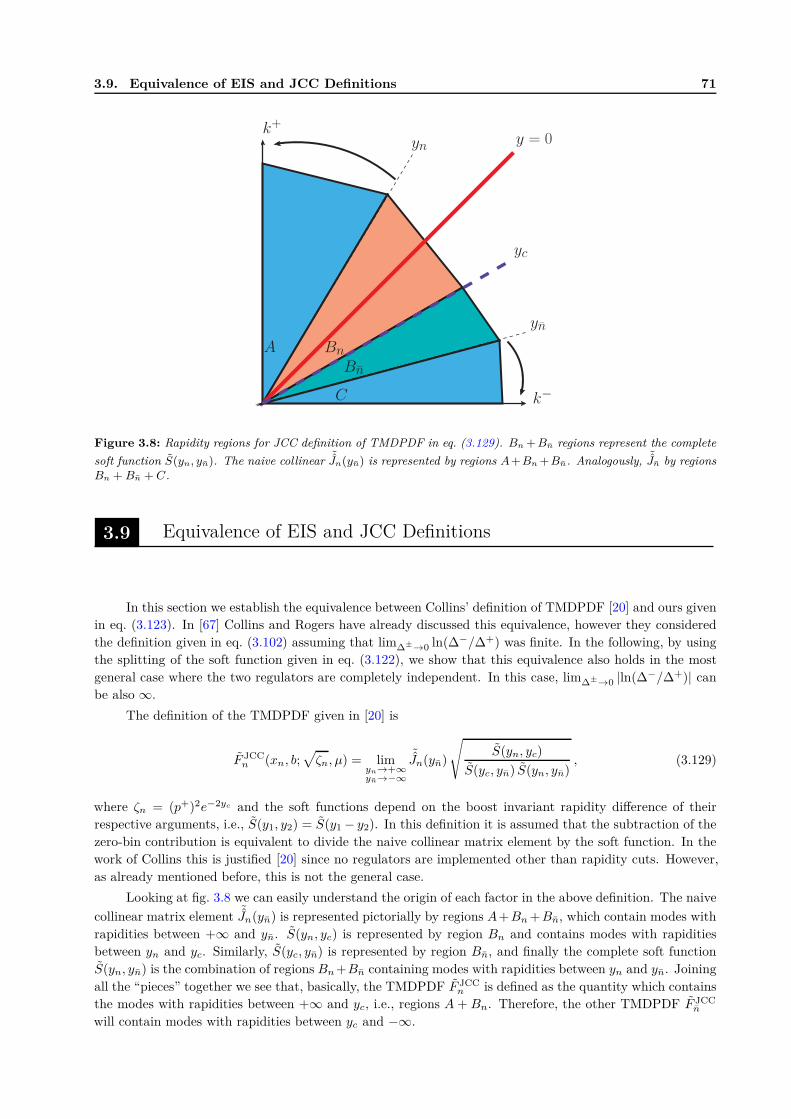
3.9. Equivalence of EIS and JCC Definitions 71
yn
yn
k+
k−
y = 0
yc
A
C
Bn
Bn
Figure 3.8: Rapidity regions for JCC definition of TMDPDF in eq. (3.129). Bn + Bn regions represent the complete
soft function S(yn, yn). The naive collinear˜Jn(yn) is represented by regions A+Bn +Bn. Analogously,
˜Jn by regions
Bn + Bn + C.
3.9 Equivalence of EIS and JCC Definitions
In this section we establish the equivalence between Collins’ definition of TMDPDF [20] and ours given
in eq. (3.123). In [67] Collins and Rogers have already discussed this equivalence, however they considered
the definition given in eq. (3.102) assuming that lim∆±→0 ln(∆−/∆+) was finite. In the following, by using
the splitting of the soft function given in eq. (3.122), we show that this equivalence also holds in the most
general case where the two regulators are completely independent. In this case, lim∆±→0 |ln(∆−/∆+)| can
be also ∞.
The definition of the TMDPDF given in [20] is
F JCCn (xn, b;
√
ζn, µ) = limyn→+∞yn→−∞
˜Jn(yn)
√
S(yn, yc)
S(yc, yn) S(yn, yn), (3.129)
where ζn = (p+)2e−2yc and the soft functions depend on the boost invariant rapidity difference of their
respective arguments, i.e., S(y1, y2) = S(y1 − y2). In this definition it is assumed that the subtraction of the
zero-bin contribution is equivalent to divide the naive collinear matrix element by the soft function. In the
work of Collins this is justified [20] since no regulators are implemented other than rapidity cuts. However,
as already mentioned before, this is not the general case.
Looking at fig. 3.8 we can easily understand the origin of each factor in the above definition. The naive
collinear matrix element˜Jn(yn) is represented pictorially by regions A+Bn +Bn, which contain modes with
rapidities between +∞ and yn. S(yn, yc) is represented by region Bn and contains modes with rapidities
between yn and yc. Similarly, S(yc, yn) is represented by region Bn, and finally the complete soft function
S(yn, yn) is the combination of regions Bn +Bn containing modes with rapidities between yn and yn. Joining
all the “pieces” together we see that, basically, the TMDPDF F JCCn is defined as the quantity which contains
the modes with rapidities between +∞ and yc, i.e., regions A + Bn. Therefore, the other TMDPDF F JCCn
will contain modes with rapidities between yc and −∞.
72 3. Drell-Yan TMD Factorization
Thus, based on the discussion above, one could naively think of defining the TMDPDF directly as
F JCC(naive)n (xn, b;
√
ζn, µ) = limyn→−∞
˜Jn(yn)
S(yc, yn). (3.130)
However, although this quantity contains modes with rapidities between +∞ and yc (regions A + Bn), it
suffers from un-cancelled self-energies at finite yc. In fact, the only purpose of the cumbersome combination
of the 3 soft functions in eq. (3.129) is to cancel the self-energy at yc, but apart from this issue, the goal
of the whole square root factor is simply to subtract S(yc, yn) from the naive collinear, i.e., region Bn in
fig. 3.8. Notice that when one insists on keeping all Wilson lines on-the-light-cone the issue of self-energies
becomes irrelevant since all self-energies cancel due to n2 = n2 = 0. Definitely, however, one needs then
to introduce a set of regulators to regularize all the non-ultraviolet divergences, i.e., IR and RD. Actually,
the introduction of such regulators in perturbative calculations is a must, at least in order to carry out
perturbative calculations beyond O(αs), where relying on cancellation of rapidity divergences between the
naive collinear and a soft function just by combining integrands (see p. 389 in [20]) becomes almost an
impossible task. Moreover it also simplifies the soft factor needed to properly define a TMDPDF, as it is
clear from eq. (3.123). The aim of the combination of collinear and soft matrix elements in eq. (3.129) is
the cancellation of the rapidity divergence when yn → −∞, as eq. (3.130) suggests, and the introduction of
more soft factors in the definition does not introduce a rapidity divergence when yn → +∞, since this is
cancelled under the square root.
It was argued in [67] the equivalence between JCC and EIS definitions of the TMDPDF by considering
the definition given in eq. (3.102). That equation can be written in terms of the naive collinear matrix
element, making more clear the comparison with JCC definition,
F oldn =
˜Jn(∆+)
√
S(
∆−
p+ ,∆+
p−
)
. (3.131)
Notice that we have written explicitly the dependence of˜Jn on its rapidity regulator ∆+, but as shown in
eq. (3.125), it also contains a pure IR dependence on ∆−. Although a different regularization method is used,
i.e., the ∆-regulator, the naive collinear matrix element˜Jn(∆+) again is represented by regions A+Bn +Bn
in fig. 3.8, containing the modes with rapidities between +∞ and yn. From the result in eq. (3.124) for
the soft function and the fact that it is boost invariant, we deduce that it depends on the boost invariant
rapidity difference
yn − yn = lnµ2Q2
∆−∆+, (3.132)
where the rapidity cutoffs are
yn = lnµp+
∆−, yn = ln
∆+
µp−. (3.133)
When taking the limits ∆± → 0 the two rapidities yn and yn take also their proper limits, yn → +∞ and
yn → −∞. In terms of these cutoffs, eq. (3.131) can be rewritten as
F oldn =
Jn(yn)√
S (yn, yn), (3.134)
which can be more easily compared to JCC definition in eq. (3.129). The authors in [67] showed that this
two definitions are equivalent if the limits of yn and yn are coordinated in such a way that yc = (yn + yn)/2
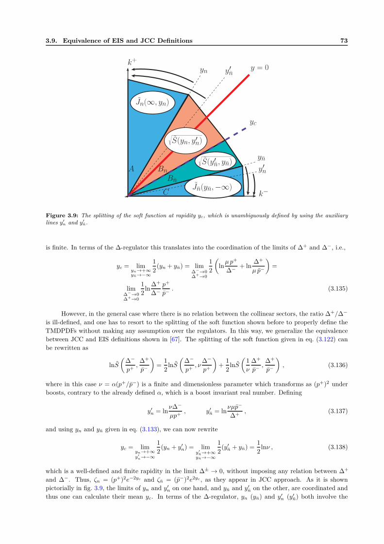
3.9. Equivalence of EIS and JCC Definitions 73
y′nyn
y′n
yn
k+
k−
Jn(∞, yn)
Jn(yn,−∞)
√
S(y′n, yn)
y = 0
yc
√
S(yn, y′n)
A
C
Bn
Bn
Figure 3.9: The splitting of the soft function at rapidity yc, which is unambiguously defined by using the auxiliarylines y′
n and y′
n.
is finite. In terms of the ∆-regulator this translates into the coordination of the limits of ∆+ and ∆−, i.e.,
yc = limyn→+∞yn→−∞
1
2(yn + yn) = lim
∆−→0∆+→0
1
2
(
lnµ p+
∆−+ ln
∆+
µ p−
)
=
lim∆−→0∆+→0
1
2ln
∆+
∆−p+
p−. (3.135)
However, in the general case where there is no relation between the collinear sectors, the ratio ∆+/∆−
is ill-defined, and one has to resort to the splitting of the soft function shown before to properly define the
TMDPDFs without making any assumption over the regulators. In this way, we generalize the equivalence
between JCC and EIS definitions shown in [67]. The splitting of the soft function given in eq. (3.122) can
be rewritten as
lnS
(
∆−
p+,
∆+
p−
)
=1
2lnS
(
∆−
p+, ν
∆−
p+
)
+1
2lnS
(
1
ν
∆+
p−,
∆+
p−
)
, (3.136)
where in this case ν = α(p+/p−) is a finite and dimensionless parameter which transforms as (p+)2 under
boosts, contrary to the already defined α, which is a boost invariant real number. Defining
y′n = lnν∆−
µp+, y′n = ln
νµp−
∆+, (3.137)
and using yn and yn given in eq. (3.133), we can now rewrite
yc = limyn→+∞y′
n→−∞
1
2(yn + y′n) = lim
y′n→+∞
yn→−∞
1
2(y′n + yn) =
1
2lnν , (3.138)
which is a well-defined and finite rapidity in the limit ∆± → 0, without imposing any relation between ∆+
and ∆−. Thus, ζn = (p+)2e−2yc and ζn = (p−)2e2yc , as they appear in JCC approach. As it is shown
pictorially in fig. 3.9, the limits of yn and y′n on one hand, and yn and y′n on the other, are coordinated and
thus one can calculate their mean yc. In terms of the ∆-regulator, yn (yn) and y′n (y′n) both involve the
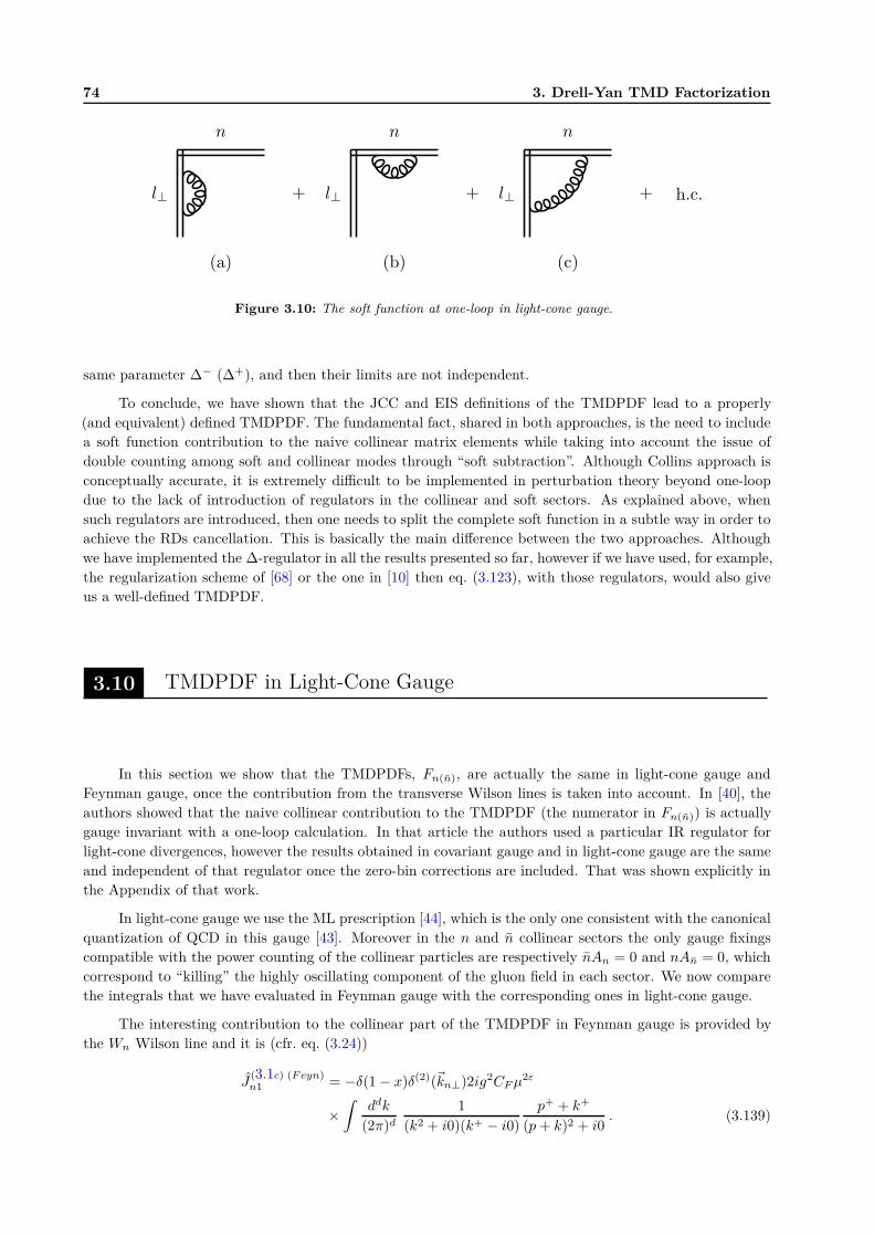
74 3. Drell-Yan TMD Factorization
Figure 3.10: The soft function at one-loop in light-cone gauge.
same parameter ∆− (∆+), and then their limits are not independent.
To conclude, we have shown that the JCC and EIS definitions of the TMDPDF lead to a properly
(and equivalent) defined TMDPDF. The fundamental fact, shared in both approaches, is the need to include
a soft function contribution to the naive collinear matrix elements while taking into account the issue of
double counting among soft and collinear modes through “soft subtraction”. Although Collins approach is
conceptually accurate, it is extremely difficult to be implemented in perturbation theory beyond one-loop
due to the lack of introduction of regulators in the collinear and soft sectors. As explained above, when
such regulators are introduced, then one needs to split the complete soft function in a subtle way in order to
achieve the RDs cancellation. This is basically the main difference between the two approaches. Although
we have implemented the ∆-regulator in all the results presented so far, however if we have used, for example,
the regularization scheme of [68] or the one in [10] then eq. (3.123), with those regulators, would also give
us a well-defined TMDPDF.
3.10 TMDPDF in Light-Cone Gauge
In this section we show that the TMDPDFs, Fn(n), are actually the same in light-cone gauge and
Feynman gauge, once the contribution from the transverse Wilson lines is taken into account. In [40], the
authors showed that the naive collinear contribution to the TMDPDF (the numerator in Fn(n)) is actually
gauge invariant with a one-loop calculation. In that article the authors used a particular IR regulator for
light-cone divergences, however the results obtained in covariant gauge and in light-cone gauge are the same
and independent of that regulator once the zero-bin corrections are included. That was shown explicitly in
the Appendix of that work.
In light-cone gauge we use the ML prescription [44], which is the only one consistent with the canonical
quantization of QCD in this gauge [43]. Moreover in the n and n collinear sectors the only gauge fixings
compatible with the power counting of the collinear particles are respectively nAn = 0 and nAn = 0, which
correspond to “killing” the highly oscillating component of the gluon field in each sector. We now compare
the integrals that we have evaluated in Feynman gauge with the corresponding ones in light-cone gauge.
The interesting contribution to the collinear part of the TMDPDF in Feynman gauge is provided by
the Wn Wilson line and it is (cfr. eq. (3.24))
J(3.1c) (F eyn)n1 = −δ(1 − x)δ(2)(~kn⊥)2ig2CFµ
2ε
×∫
ddk
(2π)d
1
(k2 + i0)(k+ − i0)
p+ + k+
(p+ k)2 + i0. (3.139)
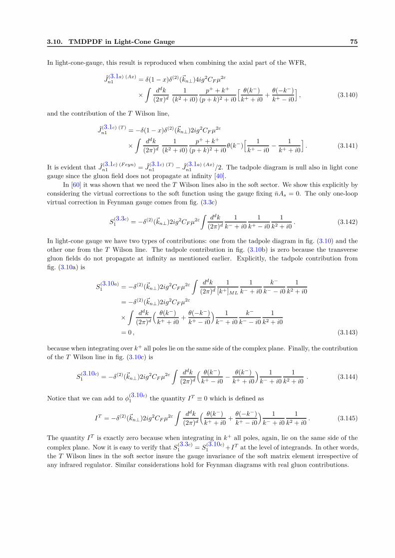
3.10. TMDPDF in Light-Cone Gauge 75
In light-cone-gauge, this result is reproduced when combining the axial part of the WFR,
J(3.1a) (Ax)n1 = δ(1 − x)δ(2)(~kn⊥)4ig2CFµ
2ε
×∫
ddk
(2π)d
1
(k2 + i0)
p+ + k+
(p+ k)2 + i0
[ θ(k−)
k+ + i0+θ(−k−)
k+ − i0
]
, (3.140)
and the contribution of the T Wilson line,
J(3.1c) (T )n1 = −δ(1 − x)δ(2)(~kn⊥)2ig2CFµ
2ε
×∫
ddk
(2π)d
1
(k2 + i0)
p+ + k+
(p+ k)2 + i0θ(k−)
[ 1
k+ − i0− 1
k+ + i0
]
. (3.141)
It is evident that J(3.1c) (F eyn)n1 = J
(3.1c) (T )n1 − J
(3.1a) (Ax)n1 /2. The tadpole diagram is null also in light cone
gauge since the gluon field does not propagate at infinity [40].
In [60] it was shown that we need the T Wilson lines also in the soft sector. We show this explicitly by
considering the virtual corrections to the soft function using the gauge fixing nAs = 0. The only one-loop
virtual correction in Feynman gauge comes from fig. (3.3c)
S(3.3c)1 = −δ(2)(~kn⊥)2ig2CFµ
2ε
∫
ddk
(2π)d
1
k− + i0
1
k+ − i0
1
k2 + i0. (3.142)
In light-cone gauge we have two types of contributions: one from the tadpole diagram in fig. (3.10) and the
other one from the T Wilson line. The tadpole contribution in fig. (3.10b) is zero because the transverse
gluon fields do not propagate at infinity as mentioned earlier. Explicitly, the tadpole contribution from
fig. (3.10a) is
S(3.10a)1 = −δ(2)(~kn⊥)2ig2CFµ
2ε
∫
ddk
(2π)d
1
[k+]ML
1
k− + i0
k−
k− − i0
1
k2 + i0
= −δ(2)(~kn⊥)2ig2CFµ2ε
×∫
ddk
(2π)d
( θ(k−)
k+ + i0+θ(−k−)
k+ − i0
) 1
k− + i0
k−
k− − i0
1
k2 + i0
= 0 , (3.143)
because when integrating over k+ all poles lie on the same side of the complex plane. Finally, the contribution
of the T Wilson line in fig. (3.10c) is
S(3.10c)1 = −δ(2)(~kn⊥)2ig2CFµ
2ε
∫
ddk
(2π)d
( θ(k−)
k+ − i0− θ(k−)
k+ + i0
) 1
k− + i0
1
k2 + i0. (3.144)
Notice that we can add to φ(3.10c)1 the quantity IT ≡ 0 which is defined as
IT = −δ(2)(~kn⊥)2ig2CFµ2ε
∫
ddk
(2π)d
( θ(k−)
k+ + i0+θ(−k−)
k+ − i0
) 1
k− + i0
1
k2 + i0. (3.145)
The quantity IT is exactly zero because when integrating in k+ all poles, again, lie on the same side of the
complex plane. Now it is easy to verify that S(3.3c)1 = S
(3.10c)1 +IT at the level of integrands. In other words,
the T Wilson lines in the soft sector insure the gauge invariance of the soft matrix element irrespective of
any infrared regulator. Similar considerations hold for Feynman diagrams with real gluon contributions.

4Evolution of TMDPDFs
In this chapter we discuss the evolution of the eight leading twist transverse momentum dependent par-
ton distribution functions, which turns out to be universal and spin independent. By using the highest order
perturbatively calculable ingredients at our disposal, we perform the resummation of the large logarithms
that appear in the evolution kernel of transverse momentum distributions up to next-to-next-to-leading log-
arithms (NNLL), thus obtaining an expression for the kernel with highly reduced model dependence. Our
results can also be obtained using the standard CSS approach when a particular choice of the b∗ prescription
is used. In this sense, and while restricted to the perturbative domain of applicability, we consider our results
as a “prediction” of the correct value of bmax which is very close to 1.5 GeV−1. We explore under which
kinematical conditions the effects of the non-perturbative region are negligible, and hence the evolution of
transverse momentum distributions can be applied in a model independent way. The application of the
kernel is illustrated by considering the unpolarized transverse momentum dependent parton distribution
function and the Sivers function.
4.1 Introduction
Transverse momentum distributions (TMDs) are needed for all processes for which intrinsic transverse
parton momenta are relevant, which form a large group. For example spin-dependent transverse momentum
asymmetries provide unique clues to clarify the internal spin, angular momentum and 3-dimensional structure
of hadrons. While operating at different energies, experiments and facilities such as HERMES, COMPASS,
JLab, Belle and BNL are pursuing intensive research programs to explore TMDs. On the theoretical side,
Sivers [69] and Collins [70] asymmetries have been intensely studied (see [71] for a review of TMDs in spin-
physics), and have attracted much attention recently [11–13, 57, 72–74]. Basically, some of the observed
spin-asymmetries are linked to the presence of gauge links in non-local correlators needed to maintain gauge
invariance.
Based on the approach to TMDPDFs developed in [75], which is a generalization of the one given
in [37, 76], and the one of Collins [20] (see also [67]), in this paper we focus on the evolution kernel for
TMDPDFs. Using the recently extracted anomalous dimension of the unpolarized quark-TMDPDF up to
O(α3s) [37, 75], and motivated by effective field theory methodology, below we offer a method to resum the
large logarithms that appear in this kernel up to NNLL. Being this kernel the same for all eight leading twist
TMDPDFs, we discuss under which conditions it can be applied in a model independent way to extract them
from data.
The study of the unpolarized TMDs was pioneered by Collins and Soper [4, 5]. Collins’ new approach
to TMDs [20] is based on defining those quantities in a way consistent with a generic factorization theorem,
extracting their anomalous dimensions and their evolution properties. This approach relies mainly on taking
some of the Wilson lines in the soft factor off-the-light-cone. When doing so, one introduces an auxiliary
parameter ζ, which specifies the measure of “off-the-light-coness”. A differential equation with respect to ζ,
the Collins-Soper evolution equation, is then derived and solved to resum large logarithms and determines
the evolution of the non-perturbative TMDs with energy. The resummation of the Collins-Soper kernel is
done following the Collins-Soper-Sterman (CSS) method [50], which is based on using an effective strong
coupling. This in turn leads to the emergence of the divergent coupling constant when hitting the Landau
pole, an issue which is then avoided by the introduction of an smooth cutoff through the bmax prescription
78 4. Evolution of TMDPDFs
and a non-perturbative model. The value of bmax and the parameters of the model can only be extracted
through fitting a resummed cross section to experimental data.
Although CSS approach is capable of giving a faithful expression for the evolution kernel in the whole
impact parameter space, the introduction of the bmax prescription leads to an overlap between the pertur-
bative and non-perturbative regions. Our aim is thus to use the highest order calculations available at the
moment to perform the resummation of large logarithms at NNLL and obtain an accurate expression for the
kernel within the perturbative domain, or in other words, a parameter free result. With this, working in the
kinematical setup where the effects of the non-perturbative region are negligible, we can achieve a model
independent kernel for all practical purposes.
The new resummation technique that we propose is based on the formalism developed in [37,75,76] and,
as we show, can also be obtained at any desired order. We find that the coherent perturbative expansion
of the running strong coupling within the resummation scheme is fundamental to get a proper evolution
kernel. In this way, being the kernel a function of the impact parameter, we characterize its perturbative
domain and study under which conditions this is the dominant one, or in other words, when the effect of
the non-perturbative large b region is negligible. Consequently, and within this setup, one can evolve the
TMDPDFs without adding any model to the evolution kernel itself. Since the final goal is to model and
extract the TMDs from data, being able to evolve them in a model independent manner allows for cleaner
parameterizations of TMDs, restricting all the model dependence to the input low energy functions. This is,
phenomenologically, the major point of our work.
Finally, comparing with the standard CSS approach and the already existing fits of the non-perturbative
Brock-Landry-Nadolsky-Yuan (BLNY) model, we find that the phenomenologically preferred value bmax =
1.5 GeV−1 [77] is more consistent with our results in the perturbative domain.
4.2 Definition of Quark-TMDPDF
Extending the work done in [37, 75], we define in impact parameter space a quark-TMDPDF of a
polarized hadron, collinear in the +z direction with momentum P and spin ~S as
Fn,αβ = Φ(0)n,αβ(∆)
√
S (∆,∆) , (4.1)
where we have used the ∆-regulator as a particular choice to regulate the rapidity divergencies. Φ(0)n,αβ stands
for a purely collinear matrix element, i.e., a matrix element which has no overlap with the soft region [34],
and it is given by the bilocal correlator
Φ(0)n,αβ = 〈P ~S|
[
ξnαWTn
]
(0+, y−, ~y⊥)[
WT†n ξnβ
]
(0) |P ~S〉 , (4.2)
and the soft function S, which encodes soft-gluon emission, is given by
S = 〈0| Tr[
ST†n ST
n
]
(0+, 0−, ~y⊥)[
ST†n ST
n
]
(0) |0〉 . (4.3)
We should mention that Fn,αβ is free from all rapidity divergences, which cancel in the combination of the
collinear and soft matrix elements in eq. (4.1), and thus the only ∆-dependence that it contains is pure
infrared [75].
To obtain the eight leading-twist quark-TMDPDFs [15,16], represented generically by Fn below, one can
simply take the trace of Fn,αβ with the Dirac structures n/2 , n/γ5
2 and iσj+γ5
2 for unpolarized, longitudinally
polarized and transversely polarized quarks, respectively, inside a polarized hadron. The superscript T
indicates transverse gauge-links Tn(n), necessary to render the matrix elements gauge-invariant [40,60]. The
definitions of collinear (Wn(n)), soft (Sn(n)) and transverse (Tn(n)) Wilson lines for DY and DIS kinematics
can be found in [37].
In section 3.7.1.1 the anomalous dimension of the unpolarized TMDPDF was given up to 3-loop order
4.3. Evolution Kernel 79
based on a factorization theorem for qT -dependent observables in a Drell-Yan process. Such factorization
theorem for the hadronic tensor can be written in impact parameter space, using the definition of the
TMDPDF given in eq. (4.1), as
M = H(Q2/µ2) Fn(xn, b;Q,µ) Fn(xn, b;Q,µ) + O(
(bQ)−1)
, (4.4)
where H is the hard coefficient encoding the physics at the probing scale Q and which is a polynomial of
only ln(Q2/µ2). This quantity is built, to all orders in perturbation theory, by considering virtual Feynman
diagrams only, and no no real gluon emission has to be considered (even in diagrams with mixed real and
gluon contributions). Moreover, the quantity H has to be free from infrared physics, no matter how the latter
is regularized. This is a general principle and it should work whether one works on or off-the-light-cone.
Since the factorization theorem given above holds, at leading-twist, also for spin-dependent observables,
one can apply the same arguments as for the unpolarized case, based on renormalization group invariance,
to get a relation between the anomalous dimensions of F and H . Since the anomalous dimensions of the
two TMDPDFs in eq. (4.4) are identical [75], then we have
γF = −1
2γH = −1
2
[
2Γcusp lnQ2
µ2+ 2γV
]
, (4.5)
where γH is known at 3-loop level [64, 65, 78] (see appendix A for more details). Γcusp stands for the well-
known cusp anomalous dimension in the fundamental representation. This crucial result can be automatically
extended to the eight leading-twist quark-TMDPDFs defined in eq. (4.1), since the anomalous dimension is
independent of spin structure.
4.3 Evolution Kernel
For spin-dependent TMDPDFs the OPE in terms of collinear PDFs fails. For instance, Sivers function
at large qT is matched onto a twist-3 collinear operator [12]. Since nowadays the phenomenological extraction
of this hadronic matrix element is not as good as for the integrated PDFs, one possibility is to resort to
non-perturbative models for the TMDPDFs themselves, fitted at low energies to experimental data in order
to make predictions for higher energy experimental probes using their evolution. Obviously, knowing this
evolution to the highest possible accuracy is very beneficial.
Starting from eq. (4.1) the evolution of a generic quark-TMDPDF is given by 1
F (x, b;Qf , µf ) = F (x, b;Qi, µi) R(b;Qi, µi, Qf , µf ) , (4.6)
where the evolution kernel R is [37, 75]
R(b;Qi, µi, Qf , µf ) = exp
{
∫ µf
µi
dµ
µγF
(
αs(µ), lnQ2
f
µ2
)}(
Q2f
Q2i
)−D(b;µi)
. (4.7)
As explained in [75], this evolution kernel is identical to the one that can be extracted from Collins’ approach
to TMDs [20] when one identifies√ζi = Qi and
√
ζf = Qf . Moreover, below we will choose µi = Qi and
µf = Qf to illustrate the application of the kernel.
The D term can be obtained by noticing that the renormalized F has to be well-defined when its
partonic version is calculated pertubatively. This means that all divergences, other than genuine long-
distance ones, have to cancel. This fundamental statement, that rapidity divergences cancel when the
collinear and soft matrix elements are combined according to eq. (4.1), allows one to extract all the Q2-
dependence from the TMDPDFs and exponentiate it with the D term (see sec. 5 in [37]), thereby summing
1Since the evolution kernel is the same for Fn and Fn, we have dropped out the n, n labels.
80 4. Evolution of TMDPDFs
large logarithms ln(Q2/q2T ). Applying renormalization group invariance to the hadronic tensor M in eq. (4.4)
we get the following relation,
dD
dlnµ= Γcusp , (4.8)
where the cusp anomalous dimension Γcusp is known at three-loops [78].
The evolution of TMDPDFs, given by the evolution kernel in eq. (4.7), is done in impact parameter
space, thus we need to Fourier transform back to momentum space and large logarithms L⊥ = ln(µ2i b
2e2γE/4)
will appear then in the D(b;µi) term when b is either large or small. These logarithms need to be resummed
in order to get sensible predictions.
The resummation that we present in the next section is valid only within the perturbative domain of
the impact parameter, b . O(1/ΛQCD), and outside this region we need a non-perturbative model for the
D(b;µi) term. However our aim is to characterize the perturbative region and isolate it as accurately as
possible using all the existing information on Γcusp and fixed order calculations of the D term. Under certain
circumstances, as we will show, we find that knowing the evolution kernel only in its perturbative domain is
enough to evolve the TMDPDFs in a model independent way. As a result, all the model dependence will be
restricted to the functional form of the low energy TMDPDFs to be extracted from fitting to data.
Below we provide the resummation of large L⊥ logarithms based on the spirit of effective field theories,
i.e., leaving fixed the scale within the strong coupling constant. Instead of solving directly the renormalization
group evolution in eq. (4.8) as it is done within the standard CSS approach, we derive a recursive relation
for the coefficients of the perturbative expansion of the D term and solve it to resum the large logarithms
to all orders.
4.3.1 Derivation of DR
Matching the perturbative expansions of the D term,
D(b;µi) =
∞∑
n=1
dn(L⊥)
(
αs(µi)
4π
)n
, L⊥ = lnµ2
i b2
4e−2γE, (4.9)
the cusp anomalous dimension Γcusp and the QCD β-function (see appendix A), one gets the following
recursive differential equation
d′n(L⊥) =1
2Γn−1 +
n−1∑
m=1
mβn−1−mdm(L⊥) , (4.10)
where d′n ≡ ddn/dL⊥. Solving this equation one can get the structure of the first three dn coefficients
d1(L⊥) =Γ0
2β0(β0L⊥) + d1(0) ,
d2(L⊥) =Γ0
4β0(β0L⊥)
2+
(
Γ1
2β0+ d1(0)
)
(β0L⊥) + d2(0) ,
d3(L⊥) =Γ0
6β0(β0L⊥)3 +
1
2
(
Γ1
β0+
1
2
Γ0β1
β20
+ 2d1(0)
)
(β0L⊥)2
+1
2
(
4d2(0) +β1
β02d1(0) +
Γ2
β0
)
(β0L⊥) + d3(0) . (4.11)
4.3. Evolution Kernel 81
From known perturbative calculations of the Drell-Yan cross section we can fix the first two finite coefficients,
as is explained in [8] 2:
d1(0) = 0 ,
d2(0) = CFCA
(
404
27− 14ζ3
)
−(
112
27
)
CFTFnf . (4.12)
Now, based on the generalization of eq. (4.11) for any value of n and after some tedious algebra, we can
derive the general form of the dn(L⊥) coefficients, being
2dn(L⊥) = (β0L⊥)n
(
Γ0
β0
1
n
)
+ (β0L⊥)n−1
(
Γ0β1
β20
(
−1 +H(1)n−1
)
|n≥3 +Γ1
β0|n≥2
)
+ (β0L⊥)n−2
(
(n− 1)2d2(0)|n≥2 + (n− 1)Γ2
2β0|n≥3 +
β1Γ1
β20
sn|n≥4
+β2
1Γ0
β30
tn|n≥5 +β2Γ0
2β20
(n− 3)|n≥4
)
+ ... , (4.13)
where
sn = (n− 1)H(1)n−2 +
1
2(5 − 3n) ,
tn =1
2
[
(1 − n)H(2)n−1 + (n+ 1) + (n− 1)(ψ(n) + γE − 2)(ψ(n) + γE)
]
. (4.14)
H(r)n =
∑nm=0 m
r is the r-th order Harmonic Number function of n and ψ(n) = Γ′(n)/Γ(n) is the digamma
function of n. Setting a = αs(µi)/(4π), X = aβ0L⊥ and using the previous result we write the D term as
DR(b;µi) =∞∑
n=1
dn(L⊥)an =
1
2
∞∑
n=1
{
Xn
(
Γ0
β0
1
n
)
+ aXn−1
(
Γ0β1
β20
(
−1 +H(1)n−1
)
|n≥3 +Γ1
β0|n≥2
)
+a2Xn−2
(
(n− 1)2d2(0)|n≥2 + (n− 1)Γ2
2β0|n≥3 +
β1Γ1
β20
sn|n≥4 +β2
1Γ0
β30
tn|n≥5
+β2Γ0
2β20
(n− 3)|n≥4
)
+ ...
}
, (4.15)
where the label R stands for “resummed”. Once we have the series of the D term organized as above, each
order in a can be summed for |X | < 1, giving
DR(b;µi) = − Γ0
2β0ln(1 −X) +
1
2
(
a
1 −X
)[
−β1Γ0
β20
(X + ln(1 − X)) +Γ1
β0X
]
+1
2
(
a
1 −X
)2 [
2d2(0) +Γ2
2β0(X(2 −X)) +
β1Γ1
2β20
(X(X − 2) − 2ln(1 −X))
+β2Γ0
2β20
X2 +β2
1Γ0
2β30
(ln2(1 −X) −X2)
]
+ ... , (4.16)
As is clear from eq. (4.16) this result for DR can be analytically continued through Borel-summation
and its validity can thus be extended to X → −∞, which corresponds to b → 0 (see eq. (4.9)). The maximum
value of X where each coefficient of an in eq. (4.16) is valid is X = 1, which corresponds to
bX(µi) =2e−γE
µiexp
[
2π
β0αs(µi)
]
. (4.17)
2In the notation of [8], our dn(0) corresponds to their dqn/2.
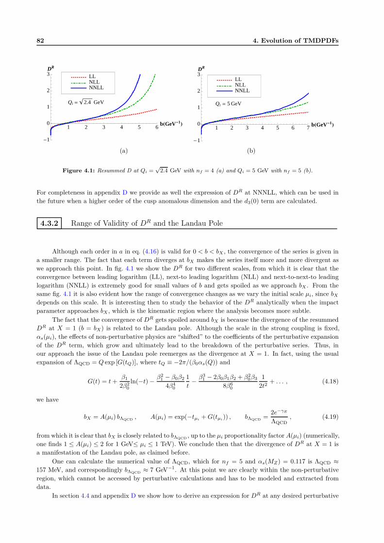
82 4. Evolution of TMDPDFs
1 2 3 4 5 6bHGeV-1L
-1
0
1
2
3DR
NNLLNLLLL
Qi = 2.4 GeV
1 2 3 4 5 6 7 bHGeV-1L
-1
0
1
2
3DR
NNLLNLLLL
Qi = 5 GeV
(a) (b)
Figure 4.1: Resummed D at Qi =√
2.4 GeV with nf = 4 (a) and Qi = 5 GeV with nf = 5 (b).
For completeness in appendix D we provide as well the expression of DR at NNNLL, which can be used in
the future when a higher order of the cusp anomalous dimension and the d3(0) term are calculated.
4.3.2 Range of Validity of DR and the Landau Pole
Although each order in a in eq. (4.16) is valid for 0 < b < bX , the convergence of the series is given in
a smaller range. The fact that each term diverges at bX makes the series itself more and more divergent as
we approach this point. In fig. 4.1 we show the DR for two different scales, from which it is clear that the
convergence between leading logarithm (LL), next-to leading logarithm (NLL) and next-to-next-to leading
logarithm (NNLL) is extremely good for small values of b and gets spoiled as we approach bX . From the
same fig. 4.1 it is also evident how the range of convergence changes as we vary the initial scale µi, since bX
depends on this scale. It is interesting then to study the behavior of the DR analytically when the impact
parameter approaches bX , which is the kinematic region where the analysis becomes more subtle.
The fact that the convergence of DR gets spoiled around bX is because the divergence of the resummed
DR at X = 1 (b = bX) is related to the Landau pole. Although the scale in the strong coupling is fixed,
αs(µi), the effects of non-perturbative physics are “shifted” to the coefficients of the perturbative expansion
of the DR term, which grow and ultimately lead to the breakdown of the perturbative series. Thus, in
our approach the issue of the Landau pole reemerges as the divergence at X = 1. In fact, using the usual
expansion of ΛQCD = Q exp [G(tQ)], where tQ ≡ −2π/(β0αs(Q)) and
G(t) = t+β1
2β20
ln(−t) − β21 − β0β2
4β40
1
t− β3
1 − 2β0β1β2 + β20β3
8β60
1
2t2+ . . . , (4.18)
we have
bX = A(µi) bΛQCD, A(µi) = exp(−tµi
+G(tµi)) , bΛQCD
=2e−γE
ΛQCD, (4.19)
from which it is clear that bX is closely related to bΛQCD, up to the µi proportionality factorA(µi) (numerically,
one finds 1 ≤ A(µi) ≤ 2 for 1 GeV≤ µi ≤ 1 TeV). We conclude then that the divergence of DR at X = 1 is
a manifestation of the Landau pole, as claimed before.
One can calculate the numerical value of ΛQCD, which for nf = 5 and αs(MZ) = 0.117 is ΛQCD ≈157 MeV, and correspondingly bΛQCD
≈ 7 GeV−1. At this point we are clearly within the non-perturbative
region, which cannot be accessed by perturbative calculations and has to be modeled and extracted from
data.
In section 4.4 and appendix D we show how to derive an expression for DR at any desired perturbative
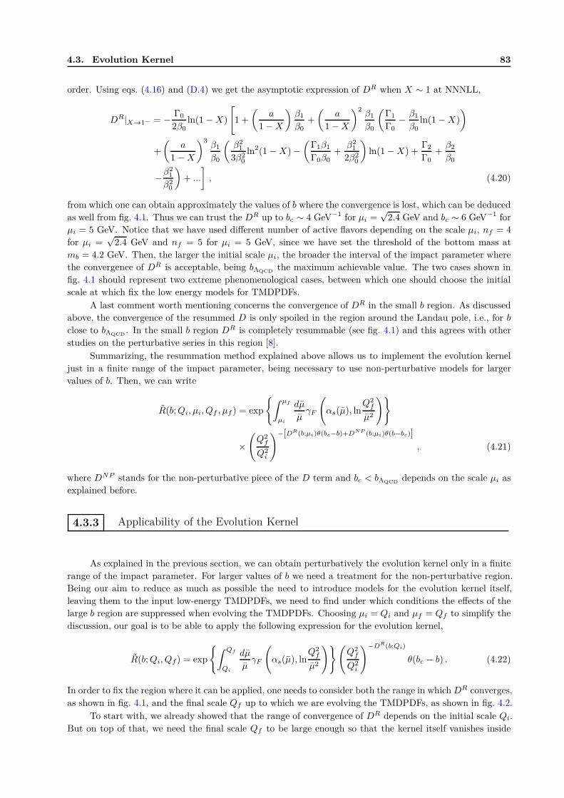
4.3. Evolution Kernel 83
order. Using eqs. (4.16) and (D.4) we get the asymptotic expression of DR when X ∼ 1 at NNNLL,
DR|X→1− = − Γ0
2β0ln(1 −X)
[
1 +
(
a
1 −X
)
β1
β0+
(
a
1 −X
)2β1
β0
(
Γ1
Γ0− β1
β0ln(1 −X)
)
+
(
a
1 −X
)3β1
β0
(
β21
3β20
ln2(1 −X) −(
Γ1β1
Γ0β0+
β21
2β20
)
ln(1 −X) +Γ2
Γ0+β2
β0
−β21
β20
)
+ ...
]
, (4.20)
from which one can obtain approximately the values of b where the convergence is lost, which can be deduced
as well from fig. 4.1. Thus we can trust the DR up to bc ∼ 4 GeV−1 for µi =√
2.4 GeV and bc ∼ 6 GeV−1 for
µi = 5 GeV. Notice that we have used different number of active flavors depending on the scale µi, nf = 4
for µi =√
2.4 GeV and nf = 5 for µi = 5 GeV, since we have set the threshold of the bottom mass at
mb = 4.2 GeV. Then, the larger the initial scale µi, the broader the interval of the impact parameter where
the convergence of DR is acceptable, being bΛQCDthe maximum achievable value. The two cases shown in
fig. 4.1 should represent two extreme phenomenological cases, between which one should choose the initial
scale at which fix the low energy models for TMDPDFs.
A last comment worth mentioning concerns the convergence of DR in the small b region. As discussed
above, the convergence of the resummed D is only spoiled in the region around the Landau pole, i.e., for b
close to bΛQCD. In the small b region DR is completely resummable (see fig. 4.1) and this agrees with other
studies on the perturbative series in this region [8].
Summarizing, the resummation method explained above allows us to implement the evolution kernel
just in a finite range of the impact parameter, being necessary to use non-perturbative models for larger
values of b. Then, we can write
R(b;Qi, µi, Qf , µf ) = exp
{
∫ µf
µi
dµ
µγF
(
αs(µ), lnQ2
f
µ2
)}
×(
Q2f
Q2i
)−[DR(b;µi)θ(bc−b)+DNP (b;µi)θ(b−bc)]
, (4.21)
where DNP stands for the non-perturbative piece of the D term and bc < bΛQCDdepends on the scale µi as
explained before.
4.3.3 Applicability of the Evolution Kernel
As explained in the previous section, we can obtain perturbatively the evolution kernel only in a finite
range of the impact parameter. For larger values of b we need a treatment for the non-perturbative region.
Being our aim to reduce as much as possible the need to introduce models for the evolution kernel itself,
leaving them to the input low-energy TMDPDFs, we need to find under which conditions the effects of the
large b region are suppressed when evolving the TMDPDFs. Choosing µi = Qi and µf = Qf to simplify the
discussion, our goal is to be able to apply the following expression for the evolution kernel,
R(b;Qi, Qf) = exp
{
∫ Qf
Qi
dµ
µγF
(
αs(µ), lnQ2
f
µ2
)}(
Q2f
Q2i
)−DR(b;Qi)
θ(bc − b) . (4.22)
In order to fix the region where it can be applied, one needs to consider both the range in which DR converges,
as shown in fig. 4.1, and the final scale Qf up to which we are evolving the TMDPDFs, as shown in fig. 4.2.
To start with, we already showed that the range of convergence of DR depends on the initial scale Qi.
But on top of that, we need the final scale Qf to be large enough so that the kernel itself vanishes inside
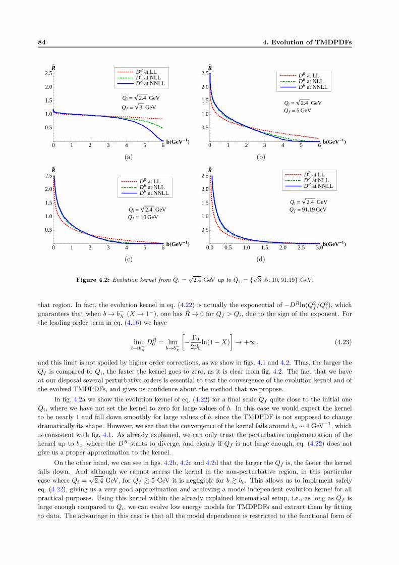
84 4. Evolution of TMDPDFs
0 1 2 3 4 5 6bHGeV-1L
0.5
1.0
1.5
2.0
2.5R�
DR at NNLLDR at NLLDR at LL
Qi = 2.4 GeV
Q f = 3 GeV
0 1 2 3 4 5 6bHGeV-1L
0.5
1.0
1.5
2.0
2.5R�
DR at NNLLDR at NLLDR at LL
Qi = 2.4 GeVQ f = 5 GeV
(a) (b)
0 1 2 3 4 5 6bHGeV-1L
0.5
1.0
1.5
2.0
2.5R�
DR at NNLLDR at NLLDR at LL
Qi = 2.4 GeVQ f = 10 GeV
0.0 0.5 1.0 1.5 2.0 2.5 3.0bHGeV-1L
0.5
1.0
1.5
2.0
2.5R�
DR at NNLLDR at NLLDR at LL
Qi = 2.4 GeVQ f = 91.19 GeV
(c) (d)
Figure 4.2: Evolution kernel from Qi =√
2.4 GeV up to Qf = {√
3 , 5 , 10, 91.19} GeV.
that region. In fact, the evolution kernel in eq. (4.22) is actually the exponential of −DRln(Q2f/Q
2i ), which
guarantees that when b → b−X (X → 1−), one has R → 0 for Qf > Qi, due to the sign of the exponent. For
the leading order term in eq. (4.16) we have
limb→b−
X
DR0 = lim
b→b−
X
[
− Γ0
2β0ln(1 −X)
]
→ +∞ , (4.23)
and this limit is not spoiled by higher order corrections, as we show in figs. 4.1 and 4.2. Thus, the larger the
Qf is compared to Qi, the faster the kernel goes to zero, as it is clear from fig. 4.2. The fact that we have
at our disposal several perturbative orders is essential to test the convergence of the evolution kernel and of
the evolved TMDPDFs, and gives us confidence about the method that we propose.
In fig. 4.2a we show the evolution kernel of eq. (4.22) for a final scale Qf quite close to the initial one
Qi, where we have not set the kernel to zero for large values of b. In this case we would expect the kernel
to be nearly 1 and fall down smoothly for large values of b, since the TMDPDF is not supposed to change
dramatically its shape. However, we see that the convergence of the kernel fails around bc ∼ 4 GeV−1, which
is consistent with fig. 4.1. As already explained, we can only trust the perturbative implementation of the
kernel up to bc, where the DR starts to diverge, and clearly if Qf is not large enough, eq. (4.22) does not
give us a proper approximation to the kernel.
On the other hand, we can see in figs. 4.2b, 4.2c and 4.2d that the larger the Qf is, the faster the kernel
falls down. And although we cannot access the kernel in the non-perturbative region, in this particular
case where Qi =√
2.4 GeV, for Qf & 5 GeV it is negligible for b & bc. This allows us to implement safely
eq. (4.22), giving us a very good approximation and achieving a model independent evolution kernel for all
practical purposes. Using this kernel within the already explained kinematical setup, i.e., as long as Qf is
large enough compared to Qi, we can evolve low energy models for TMDPDFs and extract them by fitting
to data. The advantage in this case is that all the model dependence is restricted to the functional form of
4.4. An Alternative Extraction of DR 85
Β at 1-loop
Β at 2-loop
Β at 3-loop
Β at 4-loop
1 2 3 4 5 6bHGeV-1L
-1.0
-0.5
0.5
1.0
1.5
2.0DCSSHLL L
Β at 1-loop
Β at 2-loop
Β at 3-loop
Β at 4-loop
1 2 3 4 5 6bHGeV-1L
-1.0
-0.5
0.0
0.5
1.0
1.5
2.0DR HLL L
(a)(b)
Figure 4.3: Resummed D(b; Qi =√
2.4) at LL of eqs. (4.25), (a), and (4.26), (b), with the running of the strongcoupling at various orders and decoupling coefficients included.
TMDPDFs, while the evolution is implemented perturbatively.
4.4 An Alternative Extraction of DR
The obtention of DR in eq. (4.16) was done by solving a recursive differential equation that came from
the RG-evolution of the D in eq. (4.8). In the following we show that one can derive the same result as well
by solving that differential equation as it is done within the standard CSS approach, i.e.,
D (b;Qi) = D (b;µb) +
∫ Qi
µb
dµ
µΓcusp , (4.24)
where µb = 2e−γE/b to cancel the L⊥ logarithms. For this it will be necessary to consider the running of
the strong coupling coherently with the resummation scheme.
First, we integrate eq. (4.24), getting at lowest order in perturbation theory,
D(b;Qi) = − Γ0
2β0lnαs(Qi)
αs(µb). (4.25)
Re-expressing αs(µb) in terms of αs(Qi) at the correct perturbative order, αs(µb) = αs(Q)/(1 − X), one
finds
D(b;Qi) = − Γ0
2β0ln(1 −X) , (4.26)
which coincides with the first term of the r.h.s of eq. (4.16). Repeating the same steps with higher orders
one gets that the resummed D within CSS approach given in eq. (4.24) and our case, given in eq. (4.16), are
exactly the same order by order. In appendix D we report a derivation of the same result at NLL, NNLL
and NNNLL. The expansion of the D as in eq. (4.25) at NLL, NNLL and NNNLL is in eq. (D.1). Thus,
we conclude that DR can be obtained as well within CSS approach when all terms are resummed up to its
appropriate order.
The way the evolution is usually implemented within CSS approach in the literature is described in
appendix B, and comparing fig. 4.2b and fig. B.1a one sees a difference in the two approaches. This difference
is apparent also in a numerical comparison of eq. (4.25) with respect to eq. (4.26), as shown in fig. (4.3).
The crucial point is that going from eq. (4.25) to eq. (4.26) requires that no higher order contributions from
the running of αs are included and that the number of flavors included in the running of αs(Q) and αs(µb)
is the same. In fact, even at one loop and taking αs(MZ) as the reference for the running of the strong
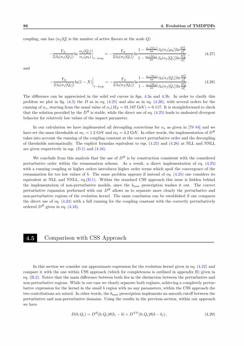
86 4. Evolution of TMDPDFs
coupling, one has (nf [Q] is the number of active flavors at the scale Q)
− Γ0
2β0(nf [Qi])lnαs(Qi)
αs(µb)
∣
∣
∣
∣
1−loop
= − Γ0
2β0(nf [Qi])ln
1 − αs(MZ )4π β0(nf [µb])ln
M2Z
µ2b
1 − αs(MZ )4π β0(nf [Qi])ln
M2Z
Q2i
, (4.27)
and
− Γ0
2β0(nf [Qi])ln(1 − X)
∣
∣
∣
∣
1−loop
= − Γ0
2β0(nf [Qi])ln
1 − αs(MZ)4π β0(nf [Qi])ln
M2Z
µ2b
1 − αs(MZ)4π β0(nf [Qi])ln
M2Z
Q2i
. (4.28)
The difference can be appreciated in the solid red curves in figs. 4.3a and 4.3b. In order to clarify this
problem we plot in fig. (4.3) the D as in eq. (4.25) and also as in eq. (4.26), with several orders for the
running of αs, starting from the usual value of αs(MZ = 91.187 GeV) = 0.117. It is straightforward to check
that the solution provided by the DR is stable, while the direct use of eq. (4.25) leads to undesired divergent
behavior for relatively low values of the impact parameter.
In our calculation we have implemented all decoupling corrections for αs as given in [79–84] and we
have set the mass thresholds at mc = 1.2 GeV and mb = 4.2 GeV. In other words, the implementation of DR
takes into account the running of the coupling constant at the correct perturbative order and the decoupling
of thresholds automatically. The explicit formulas equivalent to eqs. (4.25) and (4.26) at NLL and NNLL
are given respectively in eqs. (D.1) and (4.16).
We conclude from this analysis that the use of DR is by construction consistent with the considered
perturbative order within the resummation scheme. As a result, a direct implementation of eq. (4.25)
with a running coupling at higher orders introduces higher order terms which spoil the convergence of the
resummation for too low values of b. The same problem appears if instead of eq. (4.25) one considers its
equivalent at NLL and NNLL, eq.(D.1). Within the standard CSS approach this issue is hidden behind
the implementation of non-perturbative models, since the bmax prescription washes it out. The correct
perturbative expansion performed with our DR allows us to separate more clearly the perturbative and
non-perturbative regions of the evolution kernel. The same conclusion can be established if one compares
the direct use of eq. (4.24) with a full running for the coupling constant with the correctly perturbatively
ordered DR given in eq. (4.16).
4.5 Comparison with CSS Approach
In this section we consider our approximate expression for the evolution kernel given in eq. (4.22) and
compare it with the one within CSS approach (which for completeness is outlined in appendix B) given in
eq. (B.2). Notice that the main difference between both lies in the distinction between the perturbative and
non-perturbative regions. While in our case we clearly separate both regimes, achieving a completely pertur-
bative expression for the kernel in the small b region with no any parameters, within the CSS approach the
two contributions are mixed. In other words, the bmax prescription implements an smooth cutoff between the
perturbative and non-perturbative domains. Using the results in the previous section, within our approach
we have
D(b;Qi) = DR(b;Qi)θ(bc − b) +DNP (b;Qi)θ(b − bc) , (4.29)
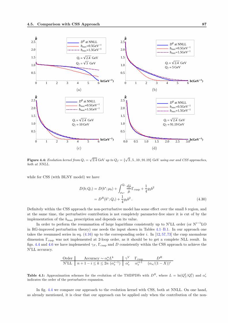
4.5. Comparison with CSS Approach 87
0 1 2 3 4 5 6bHGeV-1L
0.5
1.0
1.5
2.0
2.5R�
bmax=1.5GeV-1bmax=0.5GeV-1DR at NNLL
Qi = 2.4 GeV
Q f = 3 GeV
0 1 2 3 4 5 6bHGeV-1L
0.5
1.0
1.5
2.0
2.5R�
bmax=1.5GeV-1bmax=0.5GeV-1DR at NNLL
Qi = 2.4 GeVQ f = 5 GeV
(a) (b)
0 1 2 3 4 5 6bHGeV-1L
0.5
1.0
1.5
2.0
2.5R�
bmax=1.5GeV-1bmax=0.5GeV-1DR at NNLL
Qi = 2.4 GeVQ f = 10 GeV
0.0 0.5 1.0 1.5 2.0 2.5 3.0bHGeV-1L
0.5
1.0
1.5
2.0
2.5R�
bmax=1.5GeV-1bmax=0.5GeV-1DR at NNLL
Qi = 2.4 GeVQ f = 91.19 GeV
(c) (d)
Figure 4.4: Evolution kernel from Qi =√
2.4 GeV up to Qf = {√
3 , 5 , 10 , 91.19} GeV using our and CSS approaches,both at NNLL.
while for CSS (with BLNY model) we have
D(b;Qi) = D(b∗;µb) +
∫ Qi
µb∗
dµ
µΓcusp +
1
4g2b
2
= DR(b∗;Qi) +1
4g2b
2 . (4.30)
Definitely within the CSS approach the non-perturbative model has some effect over the small b region, and
at the same time, the perturbative contribution is not completely parameter-free since it is cut of by the
implementation of the bmax prescription and depends on its value.
In order to perform the resummation of large logarithms consistently up to NiLL order (or Ni−1LO
in RG-improved perturbation theory) one needs the input shown in Tables 4.1–B.1. In our approach one
takes the resummed series in eq. (4.16) up to the corresponding order i. In [12, 57, 73] the cusp anomalous
dimension Γcusp was not implemented at 2-loop order, as it should be to get a complete NLL result. In
figs. 4.4 and 4.6 we have implemented γF , Γcusp and D consistently within the CSS approach to achieve the
NiLL accuracy.
Order Accuracy ∼ αnsL
k γV Γcusp DR
NiLL n+ 1 − i ≤ k ≤ 2n (αi−1s ) αi
s αi+1s (αs/(1 −X))i
Table 4.1: Approximation schemes for the evolution of the TMDPDFs with DR, where L = ln(Q2f /Q2
i ) and αis
indicates the order of the perturbative expansion.
In fig. 4.4 we compare our approach to the evolution kernel with CSS, both at NNLL. On one hand,
as already mentioned, it is clear that our approach can be applied only when the contribution of the non-
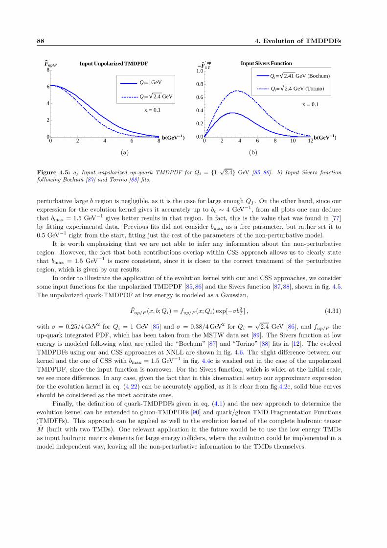
88 4. Evolution of TMDPDFs
0 2 4 6 8 bHGeV-1L0
2
4
6
8F�
up�P
Qi= 2.4 GeV
Qi=1GeV
Input Unpolarized TMDPDF
x = 0.1
0 2 4 6 8 10 12bHGeV-1L0.0
0.2
0.4
0.6
0.8
1.0-F�
1 T' up Input Sivers Function
Qi= 2.4 GeV HTorinoL
Qi= 2.41 GeV HBochumL
x = 0.1
(a) (b)
Figure 4.5: a) Input unpolarized up-quark TMDPDF for Qi = {1,√
2.4} GeV [85, 86]. b) Input Sivers functionfollowing Bochum [87] and Torino [88] fits.
perturbative large b region is negligible, as it is the case for large enough Qf . On the other hand, since our
expression for the evolution kernel gives it accurately up to bc ∼ 4 GeV−1, from all plots one can deduce
that bmax = 1.5 GeV−1 gives better results in that region. In fact, this is the value that was found in [77]
by fitting experimental data. Previous fits did not consider bmax as a free parameter, but rather set it to
0.5 GeV−1 right from the start, fitting just the rest of the parameters of the non-perturbative model.
It is worth emphasizing that we are not able to infer any information about the non-perturbative
region. However, the fact that both contributions overlap within CSS approach allows us to clearly state
that bmax = 1.5 GeV−1 is more consistent, since it is closer to the correct treatment of the perturbative
region, which is given by our results.
In order to illustrate the application of the evolution kernel with our and CSS approaches, we consider
some input functions for the unpolarized TMDPDF [85,86] and the Sivers function [87,88], shown in fig. 4.5.
The unpolarized quark-TMDPDF at low energy is modeled as a Gaussian,
Fup/P (x, b;Qi) = fup/P (x;Qi) exp[−σb2T ] , (4.31)
with σ = 0.25/4 GeV2 for Qi = 1 GeV [85] and σ = 0.38/4 GeV2 for Qi =√
2.4 GeV [86], and fup/P the
up-quark integrated PDF, which has been taken from the MSTW data set [89]. The Sivers function at low
energy is modeled following what are called the “Bochum” [87] and “Torino” [88] fits in [12]. The evolved
TMDPDFs using our and CSS approaches at NNLL are shown in fig. 4.6. The slight difference between our
kernel and the one of CSS with bmax = 1.5 GeV−1 in fig. 4.4c is washed out in the case of the unpolarized
TMDPDF, since the input function is narrower. For the Sivers function, which is wider at the initial scale,
we see more difference. In any case, given the fact that in this kinematical setup our approximate expression
for the evolution kernel in eq. (4.22) can be accurately applied, as it is clear from fig.4.2c, solid blue curves
should be considered as the most accurate ones.
Finally, the definition of quark-TMDPDFs given in eq. (4.1) and the new approach to determine the
evolution kernel can be extended to gluon-TMDPDFs [90] and quark/gluon TMD Fragmentation Functions
(TMDFFs). This approach can be applied as well to the evolution kernel of the complete hadronic tensor
M (built with two TMDs). One relevant application in the future would be to use the low energy TMDs
as input hadronic matrix elements for large energy colliders, where the evolution could be implemented in a
model independent way, leaving all the non-perturbative information to the TMDs themselves.
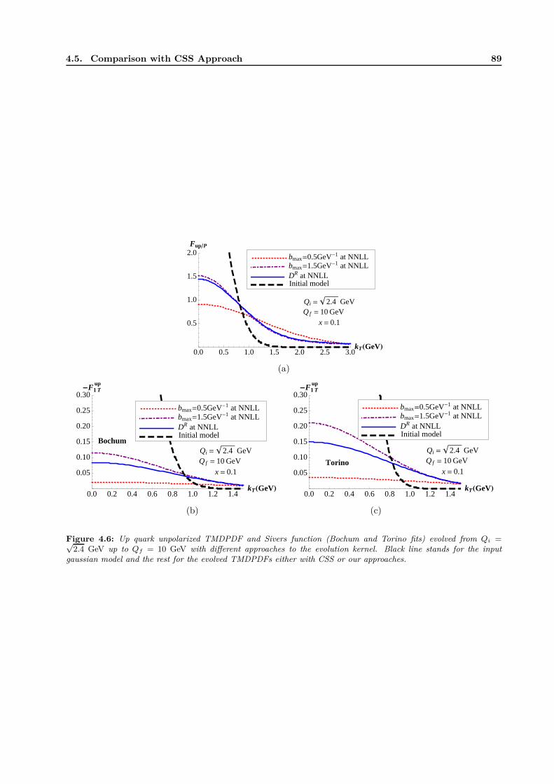
4.5. Comparison with CSS Approach 89
0.0 0.5 1.0 1.5 2.0 2.5 3.0kTHGeVL
0.5
1.0
1.5
2.0Fup�P
Initial modelDR at NNLLbmax=1.5GeV-1 at NNLLbmax=0.5GeV-1 at NNLL
Qi = 2.4 GeVQ f = 10 GeV
x = 0.1
(a)
0.0 0.2 0.4 0.6 0.8 1.0 1.2 1.4kTHGeVL
0.05
0.10
0.15
0.20
0.25
0.30-F1 T
up
Initial modelDR at NNLLbmax=1.5GeV-1 at NNLLbmax=0.5GeV-1 at NNLL
Qi = 2.4 GeVQ f = 10 GeV
x = 0.1
Bochum
0.0 0.2 0.4 0.6 0.8 1.0 1.2 1.4kTHGeVL
0.05
0.10
0.15
0.20
0.25
0.30-F1 T
up
Initial modelDR at NNLLbmax=1.5GeV-1 at NNLLbmax=0.5GeV-1 at NNLL
Qi = 2.4 GeVQ f = 10 GeV
x = 0.1Torino
(b) (c)
Figure 4.6: Up quark unpolarized TMDPDF and Sivers function (Bochum and Torino fits) evolved from Qi =√2.4 GeV up to Qf = 10 GeV with different approaches to the evolution kernel. Black line stands for the input
gaussian model and the rest for the evolved TMDPDFs either with CSS or our approaches.

5Semi-Inclusive Deep-Inelastic
Scattering TMD FactorizationIn this chapter we derive the factorization theorem for transverse-momentum dependent semi-inclusive
deep inelastic scattering (SIDIS). One of the main ingredients is the transverse-momentum dependent frag-
mentation function (TMDFF) of the measured outgoing hadron, which will be properly defined, based on
the analogous discussions done previously for the TMDPDF. Then, after performing a complete one-loop
calculation of this quantity, we will analyze its main properties, as its OPE in terms of the collinear FF and
its evolution.
5.1 Factorization of SIDIS at Small qT
As we did in chapter 3 for the case of Drell-Yan lepton pair production, below we sketch the main
steps that give us the factorization of SIDIS cross-section by using SCET technology. In SIDIS we have the
following process: l(k) + N(P ) → l′(k′) + h(P ) + X(PX), where l(l′) is the incoming (outgoing) lepton, N
is the nucleon and h is the detected hadron, for which we measure its transverse momentum. The photon
carries momentum q = k − k′, with q2 = −Q2. In terms of the commonly used invariants,
x =Q2
2P ·q , y =P ·qP ·l , z =
P ·PP ·q , (5.1)
the differential cross-section for SIDIS under one photon exchange is given by [17,91]
dσ
dx dy dz d2 ~Ph⊥
=πα2
em
2(2π)4Q4yLµνW
µν , (5.2)
where the leptonic tensor Lµν is
Lµν = 2(
kµk′ν + kνk
′µ − gµνk · k′
)
=Q2
y2
(
1 − y +y2
2
)
(−2gµν⊥ ) + ... , (5.3)
and Wµν is given by
Wµν =1
z
∑
X
∫
d4reiq · r 〈P | Jµ†(r)∣
∣XP⟩ ⟨
XP∣
∣ Jν(0) |P 〉 . (5.4)
We choose to work in the Breit frame, where the incoming hadron is traveling along the +z-direction, with
n-collinear momentum P , and the photon is n-collinear, traveling along the −z-direction. The outgoing
hadron has a momentum P mainly along the −z-direction, with a fraction z of the photon momentum in
the same direction.
The full QCD electromagnetic current,
JµQCD =
∑
q
eqψγµψ , (5.5)
92 5. Semi-Inclusive Deep-Inelastic Scattering TMD Factorization
is matched onto the SCET-qT one,
JµSCET = C(Q2/µ2)
∑
q
eq ξnWTn S
T†n γµST
n WT†n ξn , (5.6)
where the relevant Wilson lines, essential to insure gauge invariance among regular and singular gauges [60],
are:
WTn(n) = Tn(n)Wn(n) ,
Wn(x) = P exp
[
−ig∫ ∞
0
ds n ·An(x+ ns)
]
,
Tn(x) = P exp
[
−ig∫ ∞
0
dτ ~l⊥ · ~An⊥(x+,∞−, ~x⊥ +~l⊥τ)
]
,
Tn(x) = P exp
[
−ig∫ ∞
0
dτ ~l⊥ · ~An⊥(∞+, x−, ~x⊥ +~l⊥τ)
]
, (5.7)
and
STn = Tsn(sn)Sn , ST
n = Tsn(sn)Sn ,
Sn(x) = P exp
[
ig
∫ 0
−∞
ds n ·As(x+ sn)
]
,
Tsn(x) = P exp
[
ig
∫ 0
−∞
dτ ~l⊥ · ~As⊥(∞+, 0−, ~x⊥ +~l⊥τ)
]
,
Tsn(x) = P exp
[
ig
∫ 0
−∞
dτ ~l⊥ · ~As⊥(0+,∞−, ~x⊥ +~l⊥τ)
]
,
Sn(x) = P exp
[
−ig∫ ∞
0
ds n ·As(x + ns)
]
,
Tsn(x) = P exp
[
−ig∫ ∞
0
dτ ~l⊥ · ~As⊥(∞+, 0−, ~x⊥ +~l⊥τ)
]
,
Tsn(x) = P exp
[
−ig∫ ∞
0
dτ ~l⊥ · ~As⊥(0+,∞−, ~x⊥ +~l⊥τ)
]
. (5.8)
Tsn(sn) appears for the gauge choice n ·As = 0 (n ·As = 0), and the rest of the Wilson lines can be obtained
by exchanging n ↔ n and P ↔ P .
Performing standard manipulations in SCET, where the key ingredient is the decoupling of the Hilbert
space into three subspaces corresponding to collinear, anti-collinear and soft modes, we get
− 1
z
∑
X
∫
d4reiq · r 〈P | Jµ†(r)∣
∣XP⟩ ⟨
XP∣
∣Jµ(0) |P 〉 −→
|C(Q2/µ2)|2 1
Nc
∑
q
eq
∫
d4reiq · r 〈P |[
ξnWTn
]
(r)n/
2
[
WT†n ξn
]
(0) |P 〉
× 1
z
∑
X
trn/
2〈0|[
WT†n ξn
]
(r)∣
∣XP⟩ ⟨
XP∣
∣
[
ξnWTn
]
(0) |0〉
× 1
Nc〈0| Tr
[
ST†n ST
n
]
(r)[
ST†n ST
n
]
(0) |0〉 (5.9)
As in Drell-Yan process, in the frame where the incoming and outgoing quarks are collinear and anti-collinear,
respectively, the photon has a hard momentum q ∼ Q(1, 1, λ), i.e., r ∼ (1/Q)(1, 1, 1/λ). Thus, we need to
Taylor expand the previous result and consider the leading order contribution.
Taking into account the mentioned considerations and performing simple manipulations analogous to
Drell-Yan case, the factorization theorem for the hadronic tensor M (in impact parameter space) for SIDIS
5.2. Universality of the TMDPDF 93
consists of the quark-TMDPDF Ff/P , quark-TMDFF DP/f and the hard part H ,
M =∑
f
H(Q2/µ2) Fn(x, b; ζF , µ2) Dn(z, b; ζD, µ
2) , (5.10)
where the TMDPDF is defined as
Fn = J (0)n (∆−)
√
S
(
∆−
p+,
∆−
p−
)
, (5.11)
and the TMDFF as
Dn = J(0)n (∆+)
√
S
(
∆+
p+,
∆+
p−
)
. (5.12)
At the operator level, the collinear matrix element is given by
Jn(x,~kn⊥) =1
2
∫
dy−d2~y⊥(2π)3
e−i( 12
y−k+n−~y⊥ ·~kn⊥)
× 〈p|[
ξnWTn
]
(0+, y−, ~y⊥)n/
2
[
WT†n ξn
]
(0) |p〉 , (5.13)
where k+n = xP+ and the spin-average is taken. The relevant soft function is
S(~ks⊥) =
∫
d2~y⊥(2π)2
ei~y⊥ ·~ks⊥1
Nc〈0| Tr
[
ST†n ST
n
]
(0+, 0−, ~y⊥)[
ST†n ST
n
]
(0) |0〉 . (5.14)
And finally, the anti-collinear matrix element is given by
Jn(z,~kn⊥) =1
2z
∫
dy+d2~y⊥(2π)3
ei( 12
y+k−
n−~y⊥ ·~kn⊥)
×∑
X
trn/
2〈0|[
WT†n ξn
]
(y+, 0−, ~y⊥)∣
∣P X⟩ ⟨
P X∣
∣
[
ξnWTn
]
(0) |0〉 , (5.15)
where k−n = P−h /z, ~kn⊥ = ~P⊥/z and the spin average is taken.
5.2 Universality of the TMDPDF
The predictive power of perturbative QCD relies on the universality of the non-perturbative matrix
elements that enter the factorization theorems relevant for different high energy processes. Those quantities
can be extracted from a limited set of hard reactions and then applied to make predictions for other processes.
In the following we examine the universality of the TMDPDF, eq. (5.11), by considering it in two different
kinematical settings: one is for DIS and the other is for DY. We will show to first order in αs and by using
the ∆-regulator that the TMDPDF is the same in those two setups.
The difference between DIS and DY settings appears already at the level of the operator definitions of
the collinear and soft matrix elements of the TMDPDF due to the existence of different Wilson lines between
the two settings. Moreover, and since the soft function connects two collinear sectors, which are obviously
different between DIS and DY, it is not immediately clear how the universality of the TMDPDF is realized.
94 5. Semi-Inclusive Deep-Inelastic Scattering TMD Factorization
The WFR diagram (3.1a) gives
ip/Σ(3.1a)(p) = −g2CF δ(1 − x)δ(2)(~kn⊥)µ2ǫ
∫
ddk
(2π)d
−(d− 2)(p/ − k/)
[(p− k)2 + i∆−][k2 + i0]
= ip/αsCF
2πδ(1 − x)δ(2)(~kn⊥)
[
1
2εUV+
1
2ln
µ2
−i∆− +1
4
]
. (5.16)
Combined with the Hermitian conjugate diagram we get
Σ(p) = Σ(3.1a)+(3.1a)∗
(p) =αsCF
2πδ(1 − x)δ(2)(~kn⊥)
[
1
εUV+ ln
µ2
∆−+
1
2
]
, (5.17)
which contributes to the collinear matrix element with − 12 Σ(p). The W Wilson line tadpole diagram, (3.1b),
is identically 0, since n2 = 0. Diagram (3.1c) and its Hermitian conjugate give
JDIS,(3.1c)+(3.1c)∗
n1 = −2ig2CF δ(1 − x)δ(2)(~kn⊥)µ2ǫ
×∫
ddk
(2π)d
p+ + k+
[k+ + iδ+][(p+ k)2 + i∆−][k2 + i0]+ h.c.
=αsCF
2πδ(1 − x)δ(2)(~kn⊥)
×[
2
εUVlnδ+
p++
2
εUV− ln2 δ
+∆−
p+µ2− 2ln
∆−
µ2+ ln2 ∆−
µ2+ 2 +
5π2
12
]
. (5.18)
The contribution of diagrams (3.3a) and (3.3b) is zero, since (3.3a) is proportional to n2 = 0 and (3.3b) to
n2 = 0. The diagram (3.3c) and its Hermitian conjugate give
SDIS,(3.3c)+(3.3c)∗
1 = −2ig2CF δ(2)(~ks⊥)µ2ε
∫
ddk
(2π)d
1
[k+ + iδ+][k− + iδ−][k2 + i0]+ h.c.
= −αsCF
2πδ(2)(~ks⊥)
[
2
ε2UV
− 2
εUVlnδ+δ−
µ2+ ln2 δ
+δ−
µ2− π2
2
]
. (5.19)
Thus, the results for the virtual contribution to the naive collinear and soft matrix elements are
Jv,DISn1 = J
DIS,(3.1c)n1 − 1
2J
DIS,(3.1a)n1
=αsCF
2πδ(1 − x)δ(2)(~kn⊥)
×[
2
εUVln
∆+
Q2+
3
2
1
εUV− ln2 ∆+∆−
Q2µ2− 3
2ln
∆−
µ2+ ln2 ∆−
µ2+
7
4+
5π2
12
]
,
Sv,DIS1 = S
DIS,(3.3c)+(3.3c)∗
1
=αsCF
2πδ(2)(~ks⊥)
[
− 2
ε2UV
+2
εUVln
∆+∆−
Q2µ2− ln2 ∆+∆−
Q2µ2+π2
2
]
, (5.20)
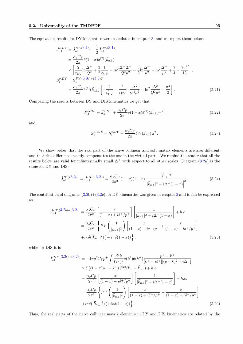
5.2. Universality of the TMDPDF 95
The equivalent results for DY kinematics were calculated in chapter 3, and we report them below:
Jv,DYn1 = J
DY,(3.1c)n1 − 1
2J
DY,(3.1a)n1
=αsCF
2πδ(1 − x)δ(2)(~kn⊥)
×[
2
εUVln
∆+
Q2+
3
2
1
εUV− ln2 ∆+∆−
Q2µ2− 3
2ln
∆−
µ2+ ln2 ∆−
µ2+
7
4− 7π2
12
]
,
Sv,DY1 = S
DY,(3.3c)+(3.3c)∗
1
=αsCF
2πδ(2)(~ks⊥)
[
− 2
ε2UV
+2
εUVln
∆2
Q2µ2− ln2 ∆2
Q2µ2− π2
2
]
, (5.21)
Comparing the results between DY and DIS kinematics we get that
Jv,DISn1 = Jv,DY
n1 +αsCF
2πδ(1 − x)δ(2)(~kn⊥)π2 , (5.22)
and
Sv,DIS1 = Sv,DY
1 +αsCF
2πδ(2)(~ks⊥)π2 . (5.23)
We show below that the real part of the naive collinear and soft matrix elements are also different,
and that this difference exactly compensates the one in the virtual parts. We remind the reader that all the
results below are valid for infinitesimally small ∆± with respect to all other scales. Diagram (3.2a) is the
same for DY and DIS,
JDY,(3.2a)n1 = J
DIS,(3.2a)n1 =
αsCF
2π2(1 − ε)(1 − x)
|~kn⊥|2∣
∣
∣|~kn⊥|2 − i∆−(1 − x)
∣
∣
∣
2 . (5.24)
The contribution of diagrams (3.2b)+(3.2c) for DY kinematics was given in chapter 3 and it can be expressed
as
JDY,(3.2b)+(3.2c)n1 =
αsCF
2π2
[
x
(1 − x) + iδ+/p+
]
[
1
|~kn⊥|2 − i∆−(1 − x)
]
+ h.c.
=αsCF
2π2
{
PV
(
1
|~kn⊥|2
)
[
x
(1 − x) + iδ+/p++
x
(1 − x) − iδ+/p+
]
+iπδ(|~kn⊥|2)(
− iπδ(1 − x))
}
, (5.25)
while for DIS it is
JDIS,(3.2b)+(3.2c)n1 = −4πg2CF p
+
∫
ddk
(2π)dδ(k2)θ(k+)
p+ − k+
[k+ − iδ+][(p− k)2 + i∆−]
× δ(
(1 − x)p+ − k+)
δ(2)(~k⊥ + ~kn⊥) + h.c.
=αsCF
2π2
[
x
(1 − x) − iδ+/p+
]
[
1
|~kn⊥|2 − i∆−(1 − x)
]
+ h.c.
=αsCF
2π2
{
PV
(
1
|~kn⊥|2
)
[
x
(1 − x) + iδ+/p++
x
(1 − x) − iδ+/p+
]
+iπδ(|~kn⊥|2) (+iπδ(1 − x))}
. (5.26)
Thus, the real parts of the naive collinear matrix elements in DY and DIS kinematics are related by the
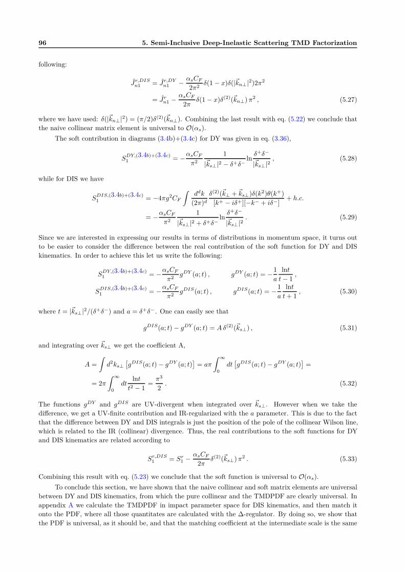
96 5. Semi-Inclusive Deep-Inelastic Scattering TMD Factorization
following:
Jr,DISn1 = Jr,DY
n1 − αsCF
2π2δ(1 − x)δ(|~kn⊥|2)2π2
= Jrn1 − αsCF
2πδ(1 − x)δ(2)(~kn⊥)π2 , (5.27)
where we have used: δ(|~kn⊥|2) = (π/2)δ(2)(~kn⊥). Combining the last result with eq. (5.22) we conclude that
the naive collinear matrix element is universal to O(αs).
The soft contribution in diagrams (3.4b)+(3.4c) for DY was given in eq. (3.36),
SDY,(3.4b)+(3.4c)1 = −αsCF
π2
1
|~ks⊥|2 − δ+δ−lnδ+δ−
|~ks⊥|2, (5.28)
while for DIS we have
SDIS,(3.4b)+(3.4c)1 = −4πg2CF
∫
ddk
(2π)d
δ(2)(~k⊥ + ~ks⊥)δ(k2)θ(k+)
[k+ − iδ+][−k− + iδ−]+ h.c.
= −αsCF
π2
1
|~ks⊥|2 + δ+δ−lnδ+δ−
|~ks⊥|2. (5.29)
Since we are interested in expressing our results in terms of distributions in momentum space, it turns out
to be easier to consider the difference between the real contribution of the soft function for DY and DIS
kinematics. In order to achieve this let us write the following:
SDY,(3.4b)+(3.4c)1 = −αsCF
π2gDY (a; t) , gDY (a; t) = −1
a
lnt
t− 1,
SDIS,(3.4b)+(3.4c)1 = −αsCF
π2gDIS(a; t) , gDIS(a; t) = −1
a
lnt
t+ 1, (5.30)
where t = |~ks⊥|2/(δ+δ−) and a = δ+δ−. One can easily see that
gDIS(a; t) − gDY (a; t) = Aδ(2)(~ks⊥) , (5.31)
and integrating over ~ks⊥ we get the coefficient A,
A =
∫
d2ks⊥
[
gDIS(a; t) − gDY (a; t)]
= aπ
∫ ∞
0
dt[
gDIS(a; t) − gDY (a; t)]
=
= 2π
∫ ∞
0
dtlnt
t2 − 1=π3
2. (5.32)
The functions gDY and gDIS are UV-divergent when integrated over ~ks⊥. However when we take the
difference, we get a UV-finite contribution and IR-regularized with the a parameter. This is due to the fact
that the difference between DY and DIS integrals is just the position of the pole of the collinear Wilson line,
which is related to the IR (collinear) divergence. Thus, the real contributions to the soft functions for DY
and DIS kinematics are related according to
Sr,DIS1 = Sr
1 − αsCF
2πδ(2)(~ks⊥)π2 . (5.33)
Combining this result with eq. (5.23) we conclude that the soft function is universal to O(αs).
To conclude this section, we have shown that the naive collinear and soft matrix elements are universal
between DY and DIS kinematics, from which the pure collinear and the TMDPDF are clearly universal. In
appendix A we calculate the TMDPDF in impact parameter space for DIS kinematics, and then match it
onto the PDF, where all those quantitates are calculated with the ∆-regulator. By doing so, we show that
the PDF is universal, as it should be, and that the matching coefficient at the intermediate scale is the same
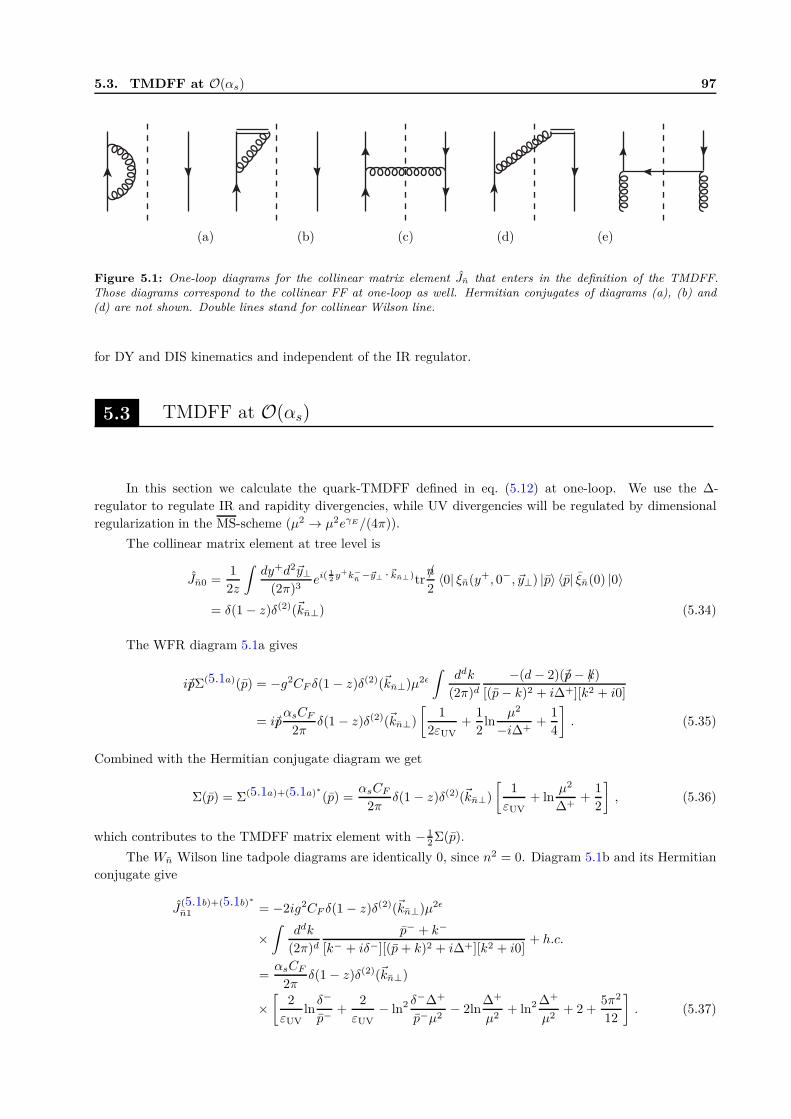
5.3. TMDFF at O(αs) 97
(a) (b) (c) (d) (e)
Figure 5.1: One-loop diagrams for the collinear matrix element Jn that enters in the definition of the TMDFF.Those diagrams correspond to the collinear FF at one-loop as well. Hermitian conjugates of diagrams (a), (b) and(d) are not shown. Double lines stand for collinear Wilson line.
for DY and DIS kinematics and independent of the IR regulator.
5.3 TMDFF at O(αs)
In this section we calculate the quark-TMDFF defined in eq. (5.12) at one-loop. We use the ∆-
regulator to regulate IR and rapidity divergencies, while UV divergencies will be regulated by dimensional
regularization in the MS-scheme (µ2 → µ2eγE/(4π)).
The collinear matrix element at tree level is
Jn0 =1
2z
∫
dy+d2~y⊥(2π)3
ei( 12
y+k−
n−~y⊥ ·~kn⊥)tr
n/
2〈0| ξn(y+, 0−, ~y⊥) |p〉 〈p| ξn(0) |0〉
= δ(1 − z)δ(2)(~kn⊥) (5.34)
The WFR diagram 5.1a gives
ip/Σ(5.1a)(p) = −g2CF δ(1 − z)δ(2)(~kn⊥)µ2ǫ
∫
ddk
(2π)d
−(d− 2)(p/− k/)
[(p− k)2 + i∆+][k2 + i0]
= ip/αsCF
2πδ(1 − z)δ(2)(~kn⊥)
[
1
2εUV+
1
2ln
µ2
−i∆++
1
4
]
. (5.35)
Combined with the Hermitian conjugate diagram we get
Σ(p) = Σ(5.1a)+(5.1a)∗
(p) =αsCF
2πδ(1 − z)δ(2)(~kn⊥)
[
1
εUV+ ln
µ2
∆++
1
2
]
, (5.36)
which contributes to the TMDFF matrix element with − 12 Σ(p).
The Wn Wilson line tadpole diagrams are identically 0, since n2 = 0. Diagram 5.1b and its Hermitian
conjugate give
J(5.1b)+(5.1b)∗
n1 = −2ig2CF δ(1 − z)δ(2)(~kn⊥)µ2ǫ
×∫
ddk
(2π)d
p− + k−
[k− + iδ−][(p+ k)2 + i∆+][k2 + i0]+ h.c.
=αsCF
2πδ(1 − z)δ(2)(~kn⊥)
×[
2
εUVlnδ−
p−+
2
εUV− ln2 δ
−∆+
p−µ2− 2ln
∆+
µ2+ ln2 ∆+
µ2+ 2 +
5π2
12
]
. (5.37)
98 5. Semi-Inclusive Deep-Inelastic Scattering TMD Factorization
Diagram 5.1c gives
J(5.1c)n1 = 2πg2CF p
− 1
z
∫
d4k
(2π)4δ(k2)θ(k−)
× 2(1 − ε)|~k⊥|2δ(
(1 − 1z )p− − k−
)
δ(2)(~k⊥ + ~kn⊥)
[(p− k)2 + i∆+][(p− k)2 − i∆+]
=αsCF
2π2
1
z
1 − z
z
|~kn⊥|2∣
∣
∣|~kn⊥|2 − i∆+(1 − 1/z)
∣
∣
∣
2 , (5.38)
where we have used(
z−1z
)2/∣
∣
z−1z
∣
∣ = 1−zz , with z ∈ [0, 1].
The sum of diagram 5.1d and its Hermitian conjugate is
J(5.1d)+(5.1d)∗
n1 = −4πg2CF p− 1
z
∫
d4k
(2π)4δ(k2)θ(k−)
× (p− − k−)δ(
(1 − 1z )p− − k−
)
δ(2)(~k⊥ + ~kn⊥)
[k− − iδ−][(p− k)2 + i∆+]+ h.c.
=αsCF
2π2
1
z2
[
1
(1 − 1/z) − iδ−/p−
]
[
−1
|~kn⊥|2 − i∆+(1 − 1/z)
]
+ h.c. , (5.39)
where we have used(
z−1z
)
/∣
∣
z−1z
∣
∣ = −1, with z ∈ [0, 1].
Now we perform the Fourier transform of the previous results to get the TMDFF in impact parameter
space. Thus, we have
˜Jn0 = δ(1 − z) . (5.40)
Σ(p) =αsCF
2πδ(1 − z)
[
1
εUV+ ln
µ2
∆++
1
2
]
. (5.41)
˜J
(5.1b)+(5.1b)∗
n1 =αsCF
2πδ(1 − z)
×[
2
εUVlnδ−
p−+
2
εUV− ln2 δ
−
p−− 2ln
δ−
p−ln
∆+
µ2− 2ln
∆+
µ2+ 2 +
5π2
12
]
. (5.42)
˜J
(5.1c)n1 =
αsCF
2π
1
z
1 − z
zln
4e−2γE
∆+ 1−zz b2
. (5.43)
5.3. TMDFF at O(αs) 99
˜J
(5.1d)+(5.1d)∗
n1 = −αsCF
2π
1
z2
[
1
(1 − 1/z) − iδ−/p−
]
ln4e−2γE
i∆+ 1−zz b2
+ h.c.
= −αsCF
2π
{[
1/z2
(1 − 1/z) − iδ−/p−+
1/z2
(1 − 1/z) + iδ−/p−
]
ln4e−2γE
∆+b2
−[ 1
z2 ln1−zz
(1 − 1/z) − iδ−/p−+
1z2 ln1−z
z
(1 − 1/z) + iδ−/p−
]
−iπ2
[
1/z2
(1 − 1/z) − iδ−/p−− 1/z2
(1 − 1/z) + iδ−/p−
]}
=αsCF
2π
[
ln4e−2γE
∆+b2
(
6z
(1 − z)++
(
9 − 2lnδ−
p−
)
δ(1 − z)
)
+2/z
(1 − z)++
(
2 + ln2 δ−
p−− π2
4
)
δ(1 − z) − π2
2δ(1 − z)
]
. (5.44)
We have used the identities in eqs. (3.30) and (3.31) to perform the Fourier transforms. Take into
account that in those identities Λ2 > 0, and this forces to take the modulus of (1 − 1/z) sometimes, which
is equivalent to write instead (1/z − 1), since z ∈ [0, 1]. We have also used the following relations for
distributions,
[
1/z2
(1 − 1/z) − iδ−/p−+
1/z2
(1 − 1/z) + iδ−/p−
]
=(1/z)2(z − 1)
(z − 1)2 + (zδ−/p−)2
=−6z
(1 − z)+−(
9 − 2lnδ−
p−
)
δ(1 − z)
[ 1z2 ln1−z
z
(1 − 1/z) − iδ−/p−+
1z2 ln1−z
z
(1 − 1/z) + iδ−/p−
]
=1
z2
z2(z − 1)ln1−zz
(z − 1)2 + (zδ−/p−)2
=2/z
(1 − z)++
(
2 + ln2 δ−
p−− π2
4
)
δ(1 − z)
[
1/z2
(1 − 1/z) − iδ−/p−− 1/z2
(1 − 1/z) + iδ−/p−
]
=(1/z)2(izδ−/p−)
(z − 1)2 + (zδ−/p−)2= iπδ(1 − z) (5.45)
Collecting all the previous partial results and the relations above, the naive collinear matrix element
in impact parameter space is then
˜Jn(z, b) = δ(1 − z) +
αsCF
2π
{
δ(1 − z)
[
2
εUVln
∆−
Q2+
3
2εUV
]
−L⊥(
1 − z
z2+
6z
(1 − z)++ 9δ(1 − z)
)
+ 2L⊥ln∆−
Q2δ(1 − z) − 1 − z
z2ln
1 − z
z+
2/z
(1 − z)+
−ln∆+
µ2
(
6z
(1 − z)++ 9δ(1 − z) − 3
2δ(1 − z) +
1 − z
z2
)
+
(
15
4− π2
3
)
δ(1 − z)
}
. (5.46)
Let us calculate now the soft function at one-loop. The soft Wilson line tadpole diagrams are identically
zero since they are proportional to either n2 = 0 or n2 = 0. Diagram 5.2a and its Hermitian conjugate give
S(5.2a)+(5.2a)∗
1 = −2ig2CF δ(2)(~ks⊥)µ2ε
∫
ddk
(2π)d
1
[k− + iδ−][k+ + iδ+][k2 + i0]+ h.c.
= −αsCF
2πδ(2)(~ks⊥)
[
2
ε2UV
− 2
εUVlnδ+δ−
µ2+ ln2 δ
+δ−
µ2− π2
2
]
. (5.47)
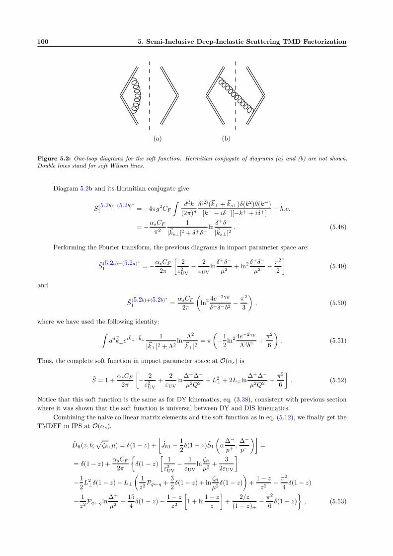
100 5. Semi-Inclusive Deep-Inelastic Scattering TMD Factorization
(a) (b)
Figure 5.2: One-loop diagrams for the soft function. Hermitian conjugate of diagrams (a) and (b) are not shown.Double lines stand for soft Wilson lines.
Diagram 5.2b and its Hermitian conjugate give
S(5.2b)+(5.2b)∗
1 = −4πg2CF
∫
ddk
(2π)d
δ(2)(~k⊥ + ~ks⊥)δ(k2)θ(k−)
[k− − iδ−][−k+ + iδ+]+ h.c.
= −αsCF
π2
1
|~ks⊥|2 + δ+δ−lnδ+δ−
|~ks⊥|2. (5.48)
Performing the Fourier transform, the previous diagrams in impact parameter space are:
S(5.2a)+(5.2a)∗
1 = −αsCF
2π
[
2
ε2UV
− 2
εUVlnδ+δ−
µ2+ ln2 δ
+δ−
µ2− π2
2
]
(5.49)
and
S(5.2b)+(5.2b)∗
1 =αsCF
2π
(
ln2 4e−2γE
δ+δ−b2− π2
3
)
, (5.50)
where we have used the following identity:
∫
dd~k⊥ei~k⊥ ·~b⊥
1
|~k⊥|2 + Λ2ln
Λ2
|~k⊥|2= π
(
−1
2ln2 4e−2γE
Λ2b2+π2
6
)
. (5.51)
Thus, the complete soft function in impact parameter space at O(αs) is
S = 1 +αsCF
2π
[
− 2
ε2UV
+2
εUVln
∆+∆−
µ2Q2+ L2
⊥ + 2L⊥ln∆+∆−
µ2Q2+π2
6
]
. (5.52)
Notice that this soft function is the same as for DY kinematics, eq. (3.38), consistent with previous section
where it was shown that the soft function is universal between DY and DIS kinematics.
Combining the naive collinear matrix elements and the soft function as in eq. (5.12), we finally get the
TMDFF in IPS at O(αs),
Dn(z, b;√
ζn, µ) = δ(1 − z) +
[
˜Jn1 − 1
2δ(1 − z)S1
(
α∆−
p+,
∆−
p−
)]
=
= δ(1 − z) +αsCF
2π
{
δ(1 − z)
[
1
ε2UV
− 1
εUVlnζn
µ2+
3
2εUV
]
−1
2L2⊥δ(1 − z) − L⊥
(
1
z2Pq←q +
3
2δ(1 − z) + ln
ζn
µ2δ(1 − z)
)
+1 − z
z2− π2
4δ(1 − z)
− 1
z2Pq←qln
∆+
µ2+
15
4δ(1 − z) − 1 − z
z2
[
1 + ln1 − z
z
]
+2/z
(1 − z)+− π2
6δ(1 − z)
}
, (5.53)
5.4. Extraction of the Hard Coefficient 101
where we have used the relations below:
2/z
(1 − z)+=
6z
(1 − z)++ 9δ(1 − z)
1
z2Pq←q =
6z
(1 − z)++ 9δ(1 − z) − 3
2δ(1 − z) +
1 − z
z2
=2
(1 − z)++
1
z2+
1
z− 3
2δ(1 − z) . (5.54)
5.4 Extraction of the Hard Coefficient
As we did in section 3.5 for DY process, let us obtain the hard coefficient for SIDIS factorization. As
explained in that section, the hard matching coefficient is calculated by subtracting the effective theory
contribution to the hadronic tensor from the one in QCD. This hadronic tensor at O(αs) in IPS can be
written in terms of the naive collinear and soft matrix elements as
M(x, z, b;Q) = H(Q2/µ2) [δ(1 − x)δ(1 − z)
+(
δ(1 − z)˜Jn1(x, b;Q,µ) + δ(1 − x)
˜Jn1(z, b;Q,µ)
−δ(1 − x)δ(1 − z)S1(b;Q))]
+O(α2s) . (5.55)
In QCD, the virtual part of M with ∆-regulator can be extracted from the calculation of the QFF for
DIS kinematics in section 1.5. Taking the result from eq. (1.93) and adding to it the Hermitian conjugate
we get,
MvQCD = δ(1 − x)δ(1 − z)
{
1 +αsCF
2π
[
−2ln2 ∆
Q2− 3ln
∆
Q2− 9
2+π2
2
]}
. (5.56)
Collecting the results in sections 5.2 and 5.3, we can write the virtual part of the naive collinear and
soft matrix elements with ∆± = ∆,
Jvn1 =
αsCF
2πδ(1 − x)
×[
2
εUVln
∆
Q2+
3
2εUV− ln2 ∆2
Q2µ2− 3
2ln
∆
µ2+ ln2 ∆
µ2+
7
4+
5π2
12
]
Jvn1 =
αsCF
2πδ(1 − z)
×[
2
εUVln
∆
Q2+
3
2εUV− ln2 ∆2
Q2µ2− 3
2ln
∆
µ2+ ln2 ∆
µ2+
7
4+
5π2
12
]
Sv1 =
αsCF
2π
[
− 2
ε2UV
+2
εUVln
∆2
Q2µ2− ln2 ∆2
Q2µ2+π2
2
]
. (5.57)
Thus, inserting the results above in eq. (5.55), the total virtual part of the hadronic tensor M in the
effective theory is
MvSCET = H(Q2/µ2)δ(1 − x)δ(1 − z)
{
1 +αsCF
2π
[
2
ε2UV
+1
εUV
(
3 + 2lnµ2
Q2
)
− 2ln2 ∆
Q2− 3ln
∆
Q2+ 3ln
µ2
Q2+ ln2 µ
2
Q2+
7
2+π2
3
]}
, (5.58)
where the UV divergences are canceled by the standard renormalization process. Notice that the IR contri-
butions in eqs. (5.56 and 5.58) are the same, as they should. Thus the matching coefficient between QCD
102 5. Semi-Inclusive Deep-Inelastic Scattering TMD Factorization
and the effective theory at scale Q is
H(Q2/µ2) = 1 +αsCF
2π
[
−3lnµ2
Q2− ln2 µ
2
Q2− 8 +
π2
6
]
. (5.59)
The above result was first derived in [39]. This result, as expected, is twice the hard part obtained in the
factorization of the QFF for DIS kinematics in section 1.5.
5.5 Refactorization: from TMDFF to FF
In this section we perform the OPE of the quark-TMDFF onto the integrated quark-FF and calculate
the matching coefficient at O(αs). The OPE of the renormalized TMDFF onto the renormalized collinear
FF is
Dn(z, b;√
ζn, µ) =
∫ 1
z
dz
z3−2εCn
(z
z, b; ζn, µ
)
dn(z;µ) , (5.60)
where the FF is defined as [5]
dn(z;µ) =zd−3
2
∫
dy+
2πei 1
2y+p−/z
× 1
2
∑
s
∑
X
trn/
2〈0|[
W †nξn
]
(y+, 0−,~0⊥)∣
∣P s,X⟩ ⟨
P s,X∣
∣
[
ξnWn
]
(0) |0〉 . (5.61)
One can then see that the matching coefficient at one loop is
Cn1 = Dn1 − dn1
z2−2ε. (5.62)
The TMDFF at one-loop was given in eq. (5.53), for which we used dimensional regularization in
d = 4 − 2ǫ dimensions and MS-scheme (µ2 → µ2eγE/(4π)) to regulate all the UV divergences, and the
∆-regulator for IR and rapidity divergencies. Thus, in order to properly obtain the matching coefficient,
below we calculate the collinear FF at O(αs) consistently with the regulators used for the TMDFF.
Notice that given the fact that we have a factor of z−2ε in the definition of the FF in eq. (5.61), it will
cancel in eq. (5.62). Thus, we will omit it in the explicit one-loop calculation performed below, both in the
collinear FF and in the extraction of the matching coefficient through eq. (5.62).
The FF at tree level is
dn0 =z
2
∫
dy+
2πei 1
2y+p−/z 1
2
∑
s
trn/
2〈0| ξn(y+, 0−,~0⊥) |p〉 〈p| ξn(0) |0〉
= δ(1 − z) (5.63)
The WFR diagram (5.1a) gives
ip/Σ(5.1a)(p) = −g2CF δ(1 − z)µ2ǫ
∫
ddk
(2π)d
−(d− 2)(p/− k/)
[(p− k)2 + i∆+][k2 + i0]
= ip/αsCF
2πδ(1 − z)
[
1
2εUV+
1
2ln
µ2
−i∆++
1
4
]
. (5.64)
Combined with the conjugate diagram we get
Σ(p) = Σ(5.1a)+(5.1a)∗
(p) =αsCF
2πδ(1 − z)
[
1
εUV+ ln
µ2
∆++
1
2
]
, (5.65)
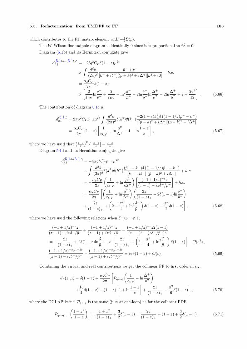
5.5. Refactorization: from TMDFF to FF 103
which contributes to the FF matrix element with − 12 Σ(p).
The W Wilson line tadpole diagram is identically 0 since it is proportional to n2 = 0.
Diagram (5.1b) and its Hermitian conjugate give
d(5.1b)+(5.1b)∗
n1 = −2ig2CF δ(1 − z)µ2ǫ
×∫
ddk
(2π)d
p− + k−
[k− + iδ−][(p+ k)2 + i∆+][k2 + i0]+ h.c.
=αsCF
2πδ(1 − z)
×[
2
εUVlnδ−
p−+
2
εUV− ln2 δ
−
p−− 2ln
δ−
p−ln
∆+
µ2− 2ln
∆+
µ2+ 2 +
5π2
12
]
. (5.66)
The contribution of diagram 5.1c is
d(5.1c)n1 = 2πg2CF p
−zµ2ε
∫
ddk
(2π)dδ(k2)θ(k−)
−2(1 − ε)k2⊥δ ((1 − 1/z)p− − k−)
[(p− k)2 + i∆+][(p− k)2 − i∆+]
=αsCF
2π(1 − z)
[
1
εUV+ ln
µ2
∆+− 1 − ln
1 − z
z
]
, (5.67)
where we have used that(
z−1z
)2/∣
∣
z−1z
∣
∣ = 1−zz .
Diagram 5.1d and its Hermitian conjugate give
d(5.1d+5.1d)n1 = −4πg2CF p
−zµ2ε
×∫
ddk
(2π)dδ(k2)θ(k−)
(p− − k−)δ ((1 − 1/z)p− − k−)
[k− − iδ−][(p− k)2 + i∆+]+ h.c.
= −αsCF
2π
(
1
εUV+ ln
µ2
i∆+
)[
(−1 + 1/z)−εz
(z − 1) − izδ−/p−
]
+ h.c.
=αsCF
2π
[(
1
εUV+ ln
µ2
∆+
)(
2z
(1 − z)+− 2δ(1 − z)ln
δ−
p−
)
+2z
(1 − z)++
(
2 − π2
4+ ln2 δ
−
p−
)
δ(1 − z) − π2
2δ(1 − z)
]
, (5.68)
where we have used the following relations when δ−/p− ≪ 1,
(−1 + 1/z)−εz
(z − 1) − izδ−/p−+
(−1 + 1/z)−εz
(z − 1) + izδ−/p−=
(−1 + 1/z)−εz2(z − 1)
(z − 1)2 + (zδ−/p−)2
= − 2z
(1 − z)++ 2δ(1 − z)ln
δ−
p−− ε
[
2z
(1 − z)++
(
2 − π2
4+ ln2 δ
−
p−
)
δ(1 − z)
]
+ O(ε2) ,
(−1 + 1/z)−εz1−2ε
(z − 1) − izδ−/p−− (−1 + 1/z)−εz1−2ε
(z − 1) + izδ−/p−= iπδ(1 − z) + O(ε) . (5.69)
Combining the virtual and real contributions we get the collinear FF to first order in αs,
dn(z;µ) = δ(1 − z) +αsCF
2π
[
Pq←q
(
1
εUV− ln
∆+
µ2
)
+15
4δ(1 − x) − (1 − z)
[
1 + ln1 − z
z
]
+2z
(1 − z)+− π2
6δ(1 − z)
]
, (5.70)
where the DGLAP kernel Pq←q is the same (just at one-loop) as for the collinear PDF,
Pq←q =
(
1 + z2
1 − z
)
+
=1 + z2
(1 − z)++
3
2δ(1 − z) =
2z
(1 − z)++ (1 − z) +
3
2δ(1 − z) . (5.71)
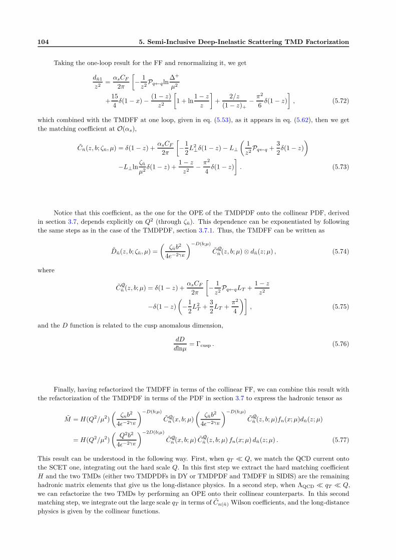
104 5. Semi-Inclusive Deep-Inelastic Scattering TMD Factorization
Taking the one-loop result for the FF and renormalizing it, we get
dn1
z2=αsCF
2π
[
− 1
z2Pq←qln
∆+
µ2
+15
4δ(1 − x) − (1 − z)
z2
[
1 + ln1 − z
z
]
+2/z
(1 − z)+− π2
6δ(1 − z)
]
, (5.72)
which combined with the TMDFF at one loop, given in eq. (5.53), as it appears in eq. (5.62), then we get
the matching coefficient at O(αs),
Cn(z, b; ζn, µ) = δ(1 − z) +αsCF
2π
[
−1
2L2⊥δ(1 − z) − L⊥
(
1
z2Pq←q +
3
2δ(1 − z)
)
−L⊥lnζn
µ2δ(1 − z) +
1 − z
z2− π2
4δ(1 − z)
]
. (5.73)
Notice that this coefficient, as the one for the OPE of the TMDPDF onto the collinear PDF, derived
in section 3.7, depends explicitly on Q2 (through ζn). This dependence can be exponentiated by following
the same steps as in the case of the TMDPDF, section 3.7.1. Thus, the TMDFF can be written as
Dn(z, b; ζn, µ) =
(
ζnb2
4e−2γE
)−D(b;µ)
CQ/n (z, b;µ) ⊗ dn(z;µ) , (5.74)
where
CQ/n (z, b;µ) = δ(1 − z) +
αsCF
2π
[
− 1
z2Pq←qLT +
1 − z
z2
−δ(1 − z)
(
−1
2L2
T +3
2LT +
π2
4
)]
, (5.75)
and the D function is related to the cusp anomalous dimension,
dD
dlnµ= Γcusp . (5.76)
Finally, having refactorized the TMDFF in terms of the collinear FF, we can combine this result with
the refactorization of the TMDPDF in terms of the PDF in section 3.7 to express the hadronic tensor as
M = H(Q2/µ2)
(
ζnb2
4ǫ−2γE
)−D(b;µ)
CQ/n (x, b;µ)
(
ζnb2
4ǫ−2γE
)−D(b;µ)
CQ/n (z, b;µ)fn(x;µ)dn(z;µ)
= H(Q2/µ2)
(
Q2b2
4ǫ−2γE
)−2D(b;µ)
CQ/n (x, b;µ) C
Q/n (z, b;µ) fn(x;µ) dn(z;µ) . (5.77)
This result can be understood in the following way. First, when qT ≪ Q, we match the QCD current onto
the SCET one, integrating out the hard scale Q. In this first step we extract the hard matching coefficient
H and the two TMDs (either two TMDPDFs in DY or TMDPDF and TMDFF in SIDIS) are the remaining
hadronic matrix elements that give us the long-distance physics. In a second step, when ΛQCD ≪ qT ≪ Q,
we can refactorize the two TMDs by performing an OPE onto their collinear counterparts. In this second
matching step, we integrate out the large scale qT in terms of Cn(n) Wilson coefficients, and the long-distance
physics is given by the collinear functions.
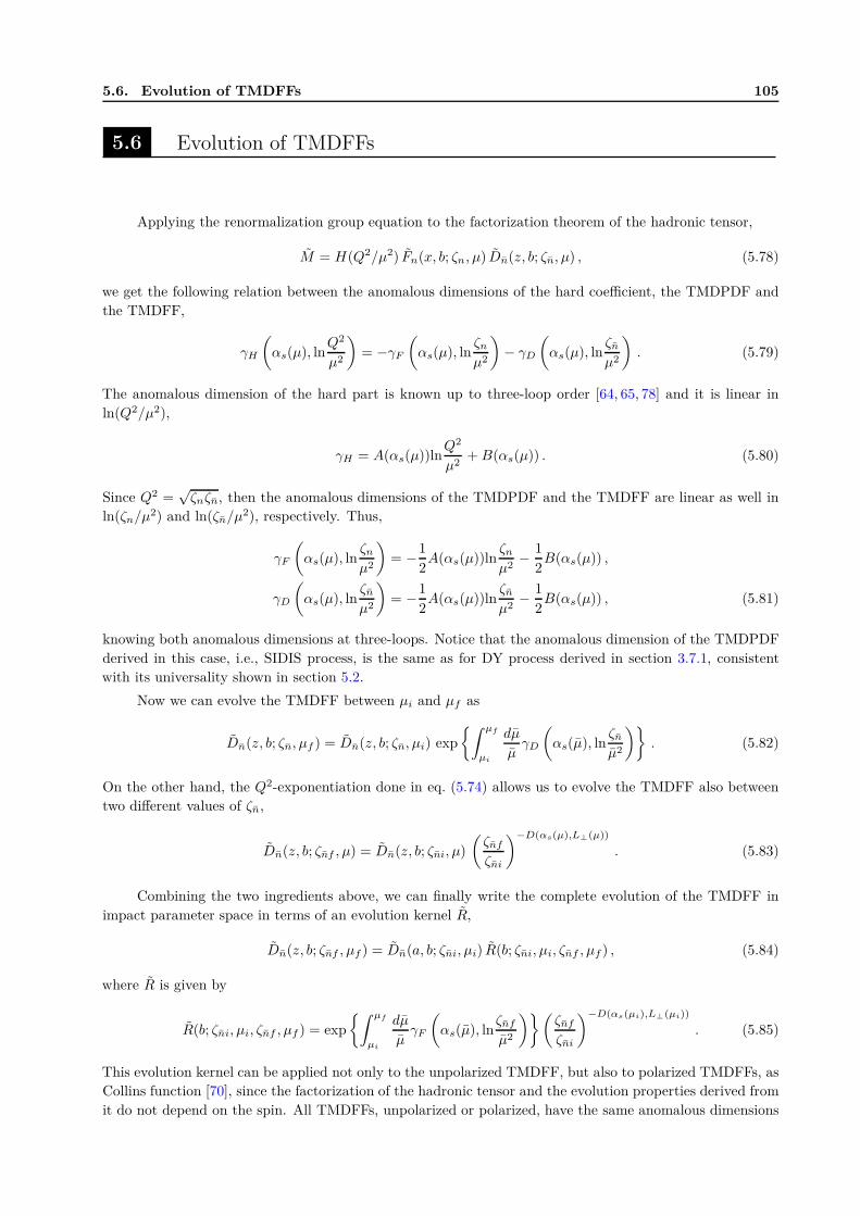
5.6. Evolution of TMDFFs 105
5.6 Evolution of TMDFFs
Applying the renormalization group equation to the factorization theorem of the hadronic tensor,
M = H(Q2/µ2) Fn(x, b; ζn, µ) Dn(z, b; ζn, µ) , (5.78)
we get the following relation between the anomalous dimensions of the hard coefficient, the TMDPDF and
the TMDFF,
γH
(
αs(µ), lnQ2
µ2
)
= −γF
(
αs(µ), lnζn
µ2
)
− γD
(
αs(µ), lnζn
µ2
)
. (5.79)
The anomalous dimension of the hard part is known up to three-loop order [64, 65, 78] and it is linear in
ln(Q2/µ2),
γH = A(αs(µ))lnQ2
µ2+B(αs(µ)) . (5.80)
Since Q2 =√ζnζn, then the anomalous dimensions of the TMDPDF and the TMDFF are linear as well in
ln(ζn/µ2) and ln(ζn/µ
2), respectively. Thus,
γF
(
αs(µ), lnζn
µ2
)
= −1
2A(αs(µ))ln
ζn
µ2− 1
2B(αs(µ)) ,
γD
(
αs(µ), lnζn
µ2
)
= −1
2A(αs(µ))ln
ζn
µ2− 1
2B(αs(µ)) , (5.81)
knowing both anomalous dimensions at three-loops. Notice that the anomalous dimension of the TMDPDF
derived in this case, i.e., SIDIS process, is the same as for DY process derived in section 3.7.1, consistent
with its universality shown in section 5.2.
Now we can evolve the TMDFF between µi and µf as
Dn(z, b; ζn, µf ) = Dn(z, b; ζn, µi) exp
{∫ µf
µi
dµ
µγD
(
αs(µ), lnζn
µ2
)}
. (5.82)
On the other hand, the Q2-exponentiation done in eq. (5.74) allows us to evolve the TMDFF also between
two different values of ζn,
Dn(z, b; ζnf , µ) = Dn(z, b; ζni, µ)
(
ζnf
ζni
)−D(αs(µ),L⊥(µ))
. (5.83)
Combining the two ingredients above, we can finally write the complete evolution of the TMDFF in
impact parameter space in terms of an evolution kernel R,
Dn(z, b; ζnf , µf ) = Dn(a, b; ζni, µi) R(b; ζni, µi, ζnf , µf ) , (5.84)
where R is given by
R(b; ζni, µi, ζnf , µf ) = exp
{∫ µf
µi
dµ
µγF
(
αs(µ), lnζnf
µ2
)}(
ζnf
ζni
)−D(αs(µi),L⊥(µi))
. (5.85)
This evolution kernel can be applied not only to the unpolarized TMDFF, but also to polarized TMDFFs, as
Collins function [70], since the factorization of the hadronic tensor and the evolution properties derived from
it do not depend on the spin. All TMDFFs, unpolarized or polarized, have the same anomalous dimensions
106 5. Semi-Inclusive Deep-Inelastic Scattering TMD Factorization
γD, known up to three-loops, and the same evolution kernel.
Finally, notice that this kernel is exactly the same as for the TMDPDFs, discussed in chapter 4. On
one hand, the anomalous dimensions of the TMDPDF, γF , and the one of the TMDFF, γD, are equal. On
the other hand, regarding the D term that allows the Q2-exponentiation, the argument is more tricky. First
of all, the differential equation fulfilled by the D is the same for both TMDs, i.e., dD/dlnµ = Γcusp. On top
of this, one has also to prove that the finite terms of the D term, that can be extracted from a perturbative
calculation of the TMDPDF or the TMDFF, are equal as well in both cases. Now, given the fact that all the
Q2-dependence in the TMDs comes solely from the presence of the soft factor in their definition, since the
pure collinear matrix elements do not depend on Q2 (see eq. (3.119) in section 3.8 and the results therein),
and considering that the soft function is universal (see discussion in section 5.2), the equality of the D term
for the TMDPDF and the TMDFF follows. Thus, all conclusions derived in chapter 4 apply as well to the
evolution of TMDFFs.
ConclusionsSoft-Collinear effective theory was formulated in covariant gauges, and it has proven to be a very
useful tool to derive factorization theorems for different processes and perform the resummation of large
logarithms in a cleaner and efficient way. However, for processes where the relevant matrix elements contain
a separation in the transverse direction, as the ones that the TMDs involve, SCET fails to provide a gauge
invariant definition for them. In chapter 2 we have explained the origin of transverse gauge links T within
SCET and studied which light-cone conditions are compatible with the power counting of the effective theory,
in such a way that the extended theory incorporates them right from the start, and all quantities built with
this theory are, for the first time, gauge invariant by definition [60]. The relevance of the T -Wilson lines in
SCET has been shown explicitly with the calculation at O(αs) of the Quark Form Factor and the TMDPDF
in Feynman and light-cone gauges.
In chapter 3 we have studied the Drell-Yan lepton pair production at small transverse momentum qT .
The analysis was carried out through the framework of the effective field theory via a two-step matching
procedure: QCD → SCET-qT → SCET-II. We established an all-order factorization theorem which allows
for a phenomenological study of DY qT spectrum to be analyzed at energies much larger than ΛQCD. When
considering the double-counting issue of the soft and the naive collinear regions properly, the obtained
factorization theorem serves as a guideline towards how the TMDPDF should be defined and what would be
its fundamental properties. In our calculations we have used Wilson lines defined on-the-light-cone and light-
cone singularities appearing in individual Feynman diagrams have been regularized with the ∆-regulator.
The fact that all Wilson lines are defined on-the-light-cone only facilitates this computation.
The two step factorization is necessary to perform the resummation of logs of qT /Q and ΛQCD/qT
respectively and we have discussed the resummation procedure in impact parameter space. In the first step
of the factorization one gets the usual structure of the cross section given in eq. (3.1). However the matrix
elements so defined are not good objects for the second factorization, because of the presence of mixed
UV/IR and rapidity divergences. All these divergences however disappear in the TMDPDF as we have
defined it. The second factorization is built up by matching the TMDPDF onto the PDF for large qT . We
have studied the Wilson coefficients that appear in the second matching which contain, in impact parameters
space, ln(Q2/µ2). We have shown that this kind of logs can be exponentiated, and thus resummed.
We have provided a definition of TMDPDFs which is gauge invariant and free from all rapidity diver-
gences including the mixed terms that spoil the renormalization of such quantities. The factorization theorem
for DY qT dependent spectrum, which is the basis leading towards defining a “TMDPDF”, is strongly be-
lieved to hold to all orders in perturbation theory and that the Glauber region is harmless. Since full QCD
quantities (like DY hadronic tensor) are free from RDs, then given the analysis presented in this work, one
can easily conclude that the RDs cancellation in the TMDPDF holds to all orders in perturbation theory.
This is important for phenomenological applications of TMDs (quarks in the case of DY or SIDIS or gluon
TMDPDFs for LHC physics) since the anomalous dimensions and the Q2-resummation kernel D [37], and
thus the evolution of individual TMDs can now be properly determined [92]. Our results can be readily
extended to define polarized and unpolarized quark and gluon TMDPDFs which could be considered as a
generalization of the one introduced in [92], as well as TMDFFs as in chapter 5.
We have also shown, by generalizing the arguments given in [67], how the TMDPDF definition, which
can be referred to as the “modified EIS” definition, is equivalent to the JCC one in the sense that both
definitions manage to cancel rapidity divergences in bi-local quark field operators separated along one light-
cone direction and also in the transverse two-dimensional space. Our definition can be readily used to carry
out perturbative calculations beyond O(αs) (with any convenient regulator, the ∆-regulator or any other
one) and calculate explicitly, for example, the anomalous dimension of polarized (such as Sivers function)
and unpolarized TMDs.
The inclusion of the square root of the soft function in the definition of the TMDPDF has important
consequences. First of all, the double counting in the factorization theorem is taken into account. Second, it
allows for the separation of UV and IR divergences in the TMDPDF. And third, even with the subtraction
of the square root of the soft function we are able to recover the PDF from the TMDPDF by integrating
over the transverse momentum.
108 Conclusions
In chapter 5 we also considered the TMDPDF with DIS kinematics and pointed out the differences
with respect to DY ones. As mentioned earlier, different Wilson lines are needed for the two kinematical
settings. However we established the universality of the TMDPDF in both regimes and argued its validity
to all orders in perturbation theory. In that chapter we followed the same steps as in chapter 3 in order to
obtain the factorization theorem for SIDIS and define the TMDFF, similarly to the TMDPDF. We performed
a complete one-loop calculation and showed the refactorization of this quantity in terms of the collinear FF,
being able to discuss the former’s evolution properties.
We have argued in chapter 4 that the evolution of leading twist TMDPDFs, both for polarized and
unpolarized ones, is driven by the same kernel [92], which can be obtained up to NNLL accuracy by using
the currently known results for the cusp anomalous dimension and the QCD β-function. For completeness,
we have provided as well an expression for the evolution kernel at NNNLL. As shown in chapter 5, this kernel
applies as well to all leading twist TMDFFs.
The evolution kernel, as a function of the impact parameter b, can be obtained in the perturbative
region without introducing any model dependence, and the resummation can be performed up to any desired
logarithmic accuracy. This resummation can be done either by solving a recursive differential equation or
by properly implementing the running of the strong coupling with renormalization scale within the standard
CSS approach. In both cases we obtained identical results. This fact is actually not surprising. The
definition of (unpolarized) TMDPDF, both in the EIS [75] and JCC [20] approaches has been shown to be
equivalent [67, 75]. If the resummation of the large logarithms is performed properly and consistently (in
terms of logarithmic accuracy) then the final results for the evolved TMDs should agree as well. We consider
this agreement as one of the major contributions of this work as it unifies a seemingly different approaches
to TMD theory and phenomenology.
As already mentioned, one of the main contributions is to give a parameter free expression for the
evolution kernel by using the highest order perturbatively calculable known ingredients, which is valid only
within the perturbative domain in the impact parameter space. On the other side, within the CSS approach
there is an overlap between the perturbative and non-perturbative contributions to the evolution kernel,
due to the implementation of a smooth cutoff through the b∗ prescription. Comparing both approaches,
we conclude that bmax = 1.5 GeV−1, which is more consistent with our results (see fig. 4.4), gives a better
description of the perturbative region within the CSS approach, as was actually found by phenomenological
fits in [77].
We have studied under which kinematical conditions the non-perturbative contribution to the kernel
is negligible, and hence our approximate expression for the kernel (in Eq. (4.22)) can be applied without
recurring to any model for all practical purposes. Given an initial scale Qi =√
2.4 GeV, at which one
would like to extract the low energy models for TMDs, if the final scale is Qf ≥ 5 GeV, then the effects of
non-perturbative physics are washed out, as is shown in Fig. 4.2. In this case, all the model dependence is
restricted to the low energy functional form of TMDs to be extracted by fitting to data.
Thus, phenomenologically, the major point of our work is to provide a scheme optimized for the
extraction of TMDs from data. Assuming that low energy models are to be extracted at scale Qi ∼ 1−2 GeV,
if data are selected with Qf > 5 GeV, then the evolution is in practice parameter free. For instance,
COMPASS, Belle or BaBar facilities can perfectly fulfill these requirements.
ATMDPDF onto PDF Matching for
SIDIS
In this appendix we calculate the matching coefficient of the TMDPDF onto the PDF for DIS kinematics
at the intermediate scale using the ∆-regulator, and show that, as expected, it does not depend on the
particular choice of the IR regulator. This matching coefficient is the same as for DY kinematics, thus
establishing its universality to first order in αs, since the PDF is universal.
For DIS kinematics the operator definition of the PDF changes, as we showed in sec. 5.2,
fDISn (x;µ) =
1
2
∫
dy−
2πe−i 1
2y−xp+ 〈p| χn(0+, y−,~0⊥)
n/
2χ†n(0+, 0−,~0⊥) |p〉
∣
∣
∣
∣
zb included
, (A.1)
where χ = W †nξn and W †n is the collinear Wilson line defined in sec. 5.2. In the following we show to first
order in αs that the PDF is universal, as expected, although its operator definition changes for DY and DIS
kinematics.
The virtual contributions to the PDF are
fDIS(3.1a)n =
αsCF
2πδ(1 − x)
[
1
εUV+ ln
µ2
∆−+
1
2
]
, (A.2)
and
fDIS,(3.1c)+(3.1c)∗
n =αsCF
2πδ(1 − x)
[
2
εUVln
∆+
Q2+
2
εUV− ln2 ∆+
Q2− 2ln
∆+
Q2ln
∆−
µ2
−2ln∆−
µ2+ 2 +
5π2
12
]
. (A.3)
The real-gluon emission contributions are
fDIS(3.2a)n = 2πg2CF p
+
∫
ddk
(2π)dδ(k2)θ(k+)
2(1 − ε)|k⊥|2δ ((1 − x)p+ − k+)
[(p− k)2 + i∆−][(p− k)2 − i∆−]
=αsCF
2π(1 − x)
[
1
εUV+ ln
µ2
∆−− 1 − ln(1 − x)
]
, (A.4)
and
fDIS(3.2b)+(3.2c)n = −4πg2CF p
+µ2ε
∫
ddk
(2π)dδ(k2)θ(k+)
p+ − k+
[k+ − iδ+][(p− k)2 + i∆−]
× δ(
(1 − x)p+ − k+)
+ h.c.
=αsCF
2π
[(
1
εUV+ ln
µ2
∆−
)(
2x
(1 − x)+− 2δ(1 − x)ln
∆+
Q2
)
−2δ(1 − x)
(
1 − π2
24− 1
2ln2 ∆+
Q2
)
− π2
2δ(1 − x)
]
, (A.5)
110 A. TMDPDF onto PDF Matching for SIDIS
Combining the virtual and real contributions we get the PDF to first order in αs
fDISn (x;µ) = QDY
n (x;µ) = δ(1 − x) +αsCF
2π
[
Pq/q
(
1
εUV− ln
∆−
µ2
)
−1
4δ(1 − x) − (1 − x) [1 + ln(1 − x)]
]
, (A.6)
which is the same as in eq. (3.78) for DY kinematics.
The virtual part of the TMDPDF for DIS kinematics is
FDIS,vn1 =
αsCF
2πδ(1 − x)
[
1
ε2UV
+1
εUV
(
3
2+ ln
µ2∆+
Q2∆−
)
−3
2ln
∆−
µ2− 1
2ln2 ∆+∆−
Q2µ2+ ln2 ∆−
µ2+
7
4+π2
6
]
. (A.7)
The real diagrams and their Fourier transforms are
JDIS(3.2a)n1 = 2πg2CF p
+
∫
ddk
(2π)dδ(k2)θ(k+)
2(1 − ε)|~k⊥|2[(p− k)2 + i∆−][(p− k)2 − i∆−]
× δ(
(1 − x)p+ − k+)
δ(2)(~k⊥ + ~kn⊥)
=2αsCF
(2π)2−2ε(1 − ε)(1 − x)
|~kn⊥|2∣
∣
∣|~kn⊥|2 − i∆−(1 − x)
∣
∣
∣
2 , (A.8)
˜J
DIS(3.2a)n1 =
αsCF
2π(1 − x) ln
4e−2γE
∆−(1 − x)b2, (A.9)
JDIS(3.2b+3.2c)n1 = −4πg2CF p
+
∫
ddk
(2π)dδ(k2)θ(k+)
p+ − k+
[k+ − iδ+][(p− k)2 + i∆−]
× δ(
(1 − x)p+ − k+)
δ(2)(~k⊥ + ~kn⊥) + h.c.
=2αsCF
(2π)2−2ε
[
x
(1 − x) − iδ+/p+
]
[
1
|~kn⊥|2 − i∆−(1 − x)
]
+ h.c. , (A.10)
˜J
DIS(3.2b+3.2c)n1 =
αsCF
2π
[
ln4e−2γE
∆−b2
(
2x
(1 − x)+− 2δ(1 − x)ln
∆+
Q2
)
− π2
2δ(1 − x)
−2δ(1 − x)
(
1 − π2
24− 1
2ln2 ∆+
Q2
)]
, (A.11)
SDIS(3.4b+3.4c)1 = −4πg2CF
∫
ddk
(2π)d
δ(2)(~k⊥ + ~kn⊥)δ(k2)θ(k+)
[k+ − iδ+][−k− + iδ−]+ h.c.
= − 4αsCF
(2π)2−2ε
1
|~kn⊥|2 + δ+δ−lnδ+δ−
|~kn⊥|2, (A.12)
SDIS(3.4b)1 =
αsCF
2π
(
ln2 4e−2γEQ2
∆+∆−b2− π2
3
)
, (A.13)
111
In the above we have used the following identity:
∫
dd~k⊥ei~k⊥ ·~b 1
|~k⊥|2 + Λ2ln
Λ2
|~k⊥|2= π
(
−1
2ln2 4e−2γE
Λ2b2+π2
6
)
, (A.14)
when Λ → 0.
Finally, setting ∆± = ∆, the total TMDPDF in impact parameter space to first order in αs can be
written as
FDISn = fDIS
n
+αsCF
2π
[
− LT Pq/q + (1 − x) − δ(1 − x)
(
1
2L2
T − 3
2LT + LT ln
Q2
µ2+π2
12
)
]
, (A.15)
where fDISn is the PDF given in eq. (A.6) and the remaining part exactly equals the OPE matching coefficient
calculated in DY kinematics, Cn(x, b,Q2, µ2).

BCSS Approach to the Evolution of
TMDsIn various works following Collins’ approach to TMDs [12, 20, 73], large L⊥ logarithms in the D term
of the evolution kernel in eq. (4.7) were resummed using the CSS approach [50], which, for the sake of
completeness and comparison, we explain below.
First, the D term is resummed using its RG-evolution in eq. (4.8),
D (b;Qi) = D (b;µb) +
∫ Qi
µb
dµ
µΓcusp , (B.1)
where large L⊥ logarithms in the D term on the right hand side are cancelled by choosing µb = 2e−γE/b.
Thus, they are resummed by evolving D from µb to Qi. However, since we need to Fourier transform back to
momentum space, at some value of b the effective coupling αs(µb) will hit the Landau pole. In fig. B.1(a) we
can see the evolution kernel R(b;Qi =√
2.4 GeV, Qf = 5 GeV) where we have used eq. (B.1) to resum the
L⊥ logarithms in D and the appearance of the Landau pole is manifest. The breakdown of the perturbative
series is driven by the running coupling αs(µb), when µb is sufficiently small.
Order Accuracy ∼ αnsL
k γV Γcusp D
NiLL n+ 1 − i ≤ k ≤ 2n (αi−1s ) αi
s αi+1s αi
s
Table B.1: Approximation schemes for the evolution of TMDs with CSS approach, where L = ln(Q2f /Q2
i ) and αis
indicates the order of the perturbative expansion.
In order to avoid this issue, CSS did not actually introduce a sharp cut-off but a smoothed one defined as
b∗ = b/√
1 + (b/bmax)2. Obviously b∗ cannot exceed bmax and the effective coupling αs(µb∗ ) does not hit the
Landau pole. As is shown in fig. B.1(b), the kernel saturates and does not present any uncontrolled behavior.
It is also worth noticing that comparing fig. B.1(a) with fig. B.1(b), we see that the implementation of the b∗
prescription has some appreciable effect in the perturbative region, which now depends on this parameter.
The lost information due to the cutoff is recovered by adding a non-perturbative model that has to
be extracted from experimental data of a measured cross section. This model not only gives the proper
information in the non-perturbative region, but also restores the correct shape of the kernel within the
perturbative domain, which was affected by the b∗ prescription. When implementing, for example, the
Brock-Landry-Nadolsky-Yuan (BLNY )model the evolution kernel can be written as
RCSS(b;Qi, Qf) = exp
{
∫ Qf
Qi
dµ
µγF
(
αs(µ), lnQ2
f
µ2
)}(
Q2f
Q2i
)−[D(b∗;Qi)+ 14
g2b2]
, (B.2)
where D(b∗;Qi) is resummed using eq. (B.1). In this model g2 = 0.68 GeV2 for bmax = 0.5 GeV−1 [93]
and g2 = 0.184 GeV2 for bmax = 1.5 GeV−1 [77]. From the theoretical point of view these two choices are
legitimate and they can be used to define the model dependence of the final result. However considering bmax
as a fitting parameter the choice of bmax = 1.5 GeV−1 should be preferred according to ref. [77]. Fig. B.1(c)
shows the complete evolution kernel with the CSS approach, eq. (B.2), while implementing the BLNY model.
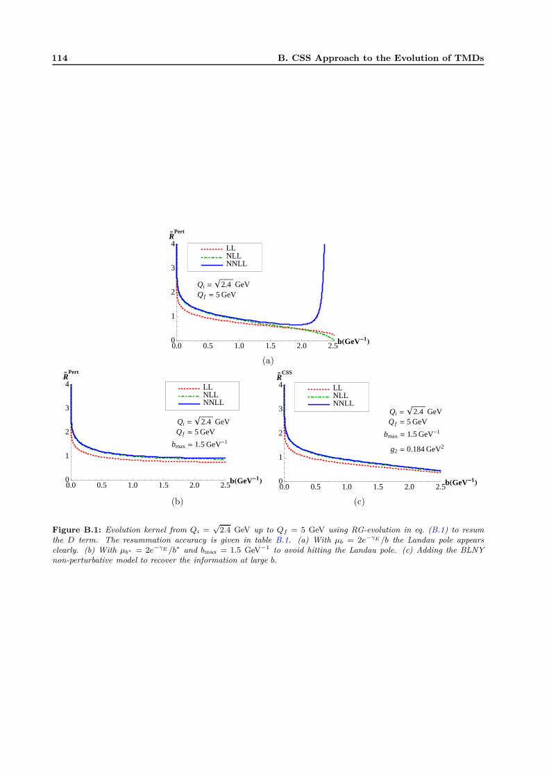
114 B. CSS Approach to the Evolution of TMDs
0.0 0.5 1.0 1.5 2.0 2.5bHGeV-1L0
1
2
3
4R� Pert
NNLLNLLLL
Qi = 2.4 GeVQ f = 5 GeV
(a)
0.0 0.5 1.0 1.5 2.0 2.5bHGeV-1L0
1
2
3
4R� Pert
Qi = 2.4 GeVQ f = 5 GeV
bmax = 1.5 GeV-1
NNLLNLLLL
0.0 0.5 1.0 1.5 2.0 2.5bHGeV-1L0
1
2
3
4R� CSS
NNLLNLLLL
Qi = 2.4 GeVQ f = 5 GeV
bmax = 1.5 GeV-1
g2 = 0.184 GeV2
(b) (c)
Figure B.1: Evolution kernel from Qi =√
2.4 GeV up to Qf = 5 GeV using RG-evolution in eq. (B.1) to resumthe D term. The resummation accuracy is given in table B.1. (a) With µb = 2e−γE /b the Landau pole appearsclearly. (b) With µb∗ = 2e−γE /b∗ and bmax = 1.5 GeV−1 to avoid hitting the Landau pole. (c) Adding the BLNYnon-perturbative model to recover the information at large b.
C
Evolution of the Hard Matching
Coefficient
The evolution of the hard matching coefficient CV , where H = |CV |2, is given by
d
dlnµlnCV (Q2/µ2) = γCV
(
αs(µ), lnQ2
µ2
)
, γCV= Γcusp(αs) ln
Q2
µ2+ γV (αs) , (C.1)
where the cusp term is related to the evolution of the Sudakov double logarithms and the remaining term
with the evolution of single logarithms. The exact solution of this equation is
CV (Q2/µ2f) = CV (Q2/µ2
i ) exp
[∫ µf
µi
dµ
µγCV
(
αs(µ), lnQ2
µ2
)]
= CV (Q2/µ2i ) exp
[
∫ αs(µf )
αs(µi)
dαs
β(αs)γCV
(αs)
]
, (C.2)
where we have used that d/dlnµ = β(αs) d/dαs, where β(αs) = dαs/dlnµ is the QCD β-function.
Below we give the expressions for the anomalous dimensions and the QCD β-function, in the MS
renormalization scheme. We use the following expansions:
Γcusp =∞∑
n=1
Γn−1
(αs
4π
)n
, γV =∞∑
n=1
γVn
(αs
4π
)n
, β = −2αs
∞∑
n=1
βn−1
(αs
4π
)n
. (C.3)
The coefficients for the cusp anomalous dimension Γcusp are
Γ0 = 4CF ,
Γ1 = 4CF
[(
67
9− π2
3
)
CA − 20
9TFnf
]
,
Γ2 = 4CF
[
C2A
(
245
6− 134π2
27+
11π4
45+
22
3ζ3
)
+ CATFnf
(
−418
27+
40π2
27− 56
3ζ3
)
+CFTFnf
(
−55
3+ 16ζ3
)
− 16
27T 2
Fn2f
]
. (C.4)
The anomalous dimension γV can be determined up to three-loop order from the partial three-loop expression
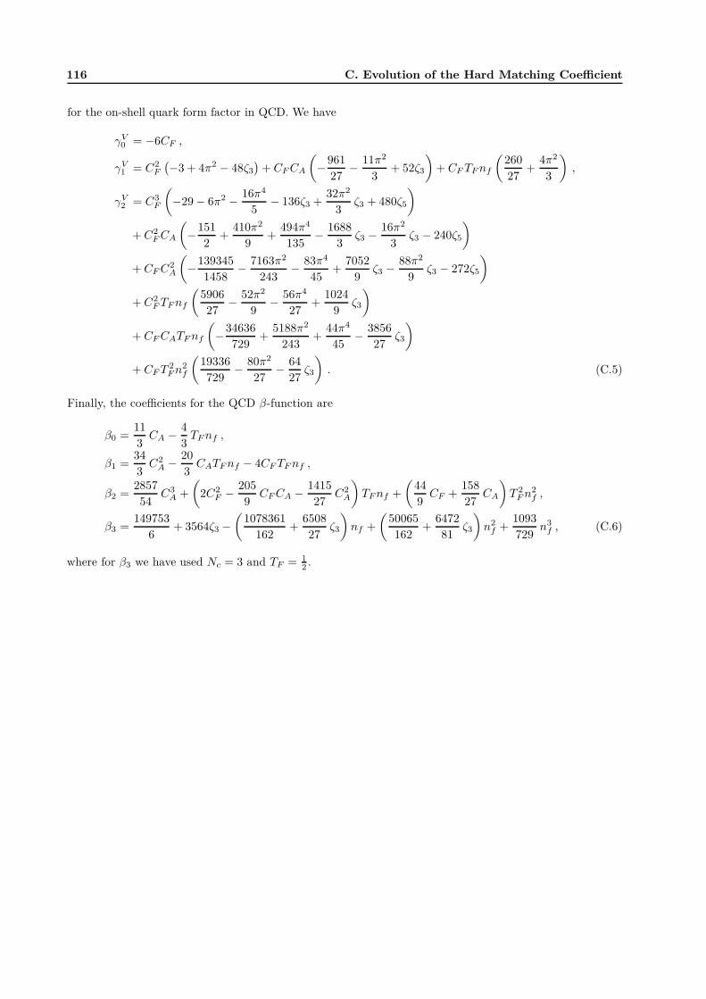
116 C. Evolution of the Hard Matching Coefficient
for the on-shell quark form factor in QCD. We have
γV0 = −6CF ,
γV1 = C2
F
(
−3 + 4π2 − 48ζ3
)
+ CFCA
(
−961
27− 11π2
3+ 52ζ3
)
+ CFTFnf
(
260
27+
4π2
3
)
,
γV2 = C3
F
(
−29 − 6π2 − 16π4
5− 136ζ3 +
32π2
3ζ3 + 480ζ5
)
+ C2FCA
(
−151
2+
410π2
9+
494π4
135− 1688
3ζ3 − 16π2
3ζ3 − 240ζ5
)
+ CFC2A
(
−139345
1458− 7163π2
243− 83π4
45+
7052
9ζ3 − 88π2
9ζ3 − 272ζ5
)
+ C2FTFnf
(
5906
27− 52π2
9− 56π4
27+
1024
9ζ3
)
+ CFCATFnf
(
−34636
729+
5188π2
243+
44π4
45− 3856
27ζ3
)
+ CFT2Fn
2f
(
19336
729− 80π2
27− 64
27ζ3
)
. (C.5)
Finally, the coefficients for the QCD β-function are
β0 =11
3CA − 4
3TFnf ,
β1 =34
3C2
A − 20
3CATFnf − 4CFTFnf ,
β2 =2857
54C3
A +
(
2C2F − 205
9CFCA − 1415
27C2
A
)
TFnf +
(
44
9CF +
158
27CA
)
T 2Fn
2f ,
β3 =149753
6+ 3564ζ3 −
(
1078361
162+
6508
27ζ3
)
nf +
(
50065
162+
6472
81ζ3
)
n2f +
1093
729n3
f , (C.6)
where for β3 we have used Nc = 3 and TF = 12 .
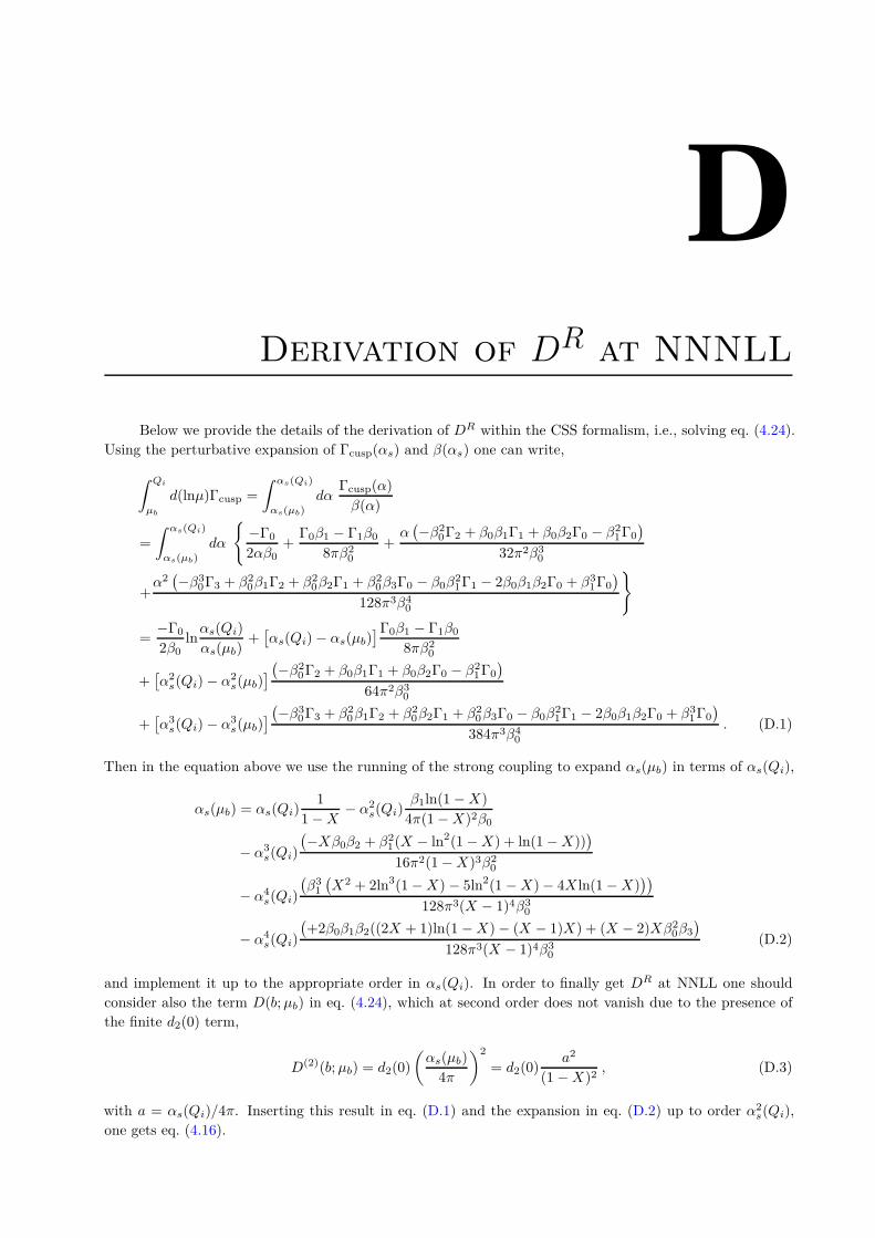
DDerivation of DR at NNNLL
Below we provide the details of the derivation of DR within the CSS formalism, i.e., solving eq. (4.24).
Using the perturbative expansion of Γcusp(αs) and β(αs) one can write,
∫ Qi
µb
d(lnµ)Γcusp =
∫ αs(Qi)
αs(µb)
dαΓcusp(α)
β(α)
=
∫ αs(Qi)
αs(µb)
dα
{
−Γ0
2αβ0+
Γ0β1 − Γ1β0
8πβ20
+α(
−β20Γ2 + β0β1Γ1 + β0β2Γ0 − β2
1Γ0
)
32π2β30
+α2(
−β30Γ3 + β2
0β1Γ2 + β20β2Γ1 + β2
0β3Γ0 − β0β21Γ1 − 2β0β1β2Γ0 + β3
1Γ0
)
128π3β40
}
=−Γ0
2β0lnαs(Qi)
αs(µb)+[
αs(Qi) − αs(µb)]Γ0β1 − Γ1β0
8πβ20
+[
α2s(Qi) − α2
s(µb)]
(
−β20Γ2 + β0β1Γ1 + β0β2Γ0 − β2
1Γ0
)
64π2β30
+[
α3s(Qi) − α3
s(µb)]
(
−β30Γ3 + β2
0β1Γ2 + β20β2Γ1 + β2
0β3Γ0 − β0β21Γ1 − 2β0β1β2Γ0 + β3
1Γ0
)
384π3β40
. (D.1)
Then in the equation above we use the running of the strong coupling to expand αs(µb) in terms of αs(Qi),
αs(µb) = αs(Qi)1
1 −X− α2
s(Qi)β1ln(1 −X)
4π(1 −X)2β0
− α3s(Qi)
(
−Xβ0β2 + β21(X − ln2(1 −X) + ln(1 −X))
)
16π2(1 −X)3β20
− α4s(Qi)
(
β31
(
X2 + 2ln3(1 −X) − 5ln2(1 −X) − 4X ln(1 −X)))
128π3(X − 1)4β30
− α4s(Qi)
(
+2β0β1β2((2X + 1)ln(1 −X) − (X − 1)X) + (X − 2)Xβ20β3
)
128π3(X − 1)4β30
(D.2)
and implement it up to the appropriate order in αs(Qi). In order to finally get DR at NNLL one should
consider also the term D(b;µb) in eq. (4.24), which at second order does not vanish due to the presence of
the finite d2(0) term,
D(2)(b;µb) = d2(0)
(
αs(µb)
4π
)2
= d2(0)a2
(1 −X)2, (D.3)
with a = αs(Qi)/4π. Inserting this result in eq. (D.1) and the expansion in eq. (D.2) up to order α2s(Qi),
one gets eq. (4.16).
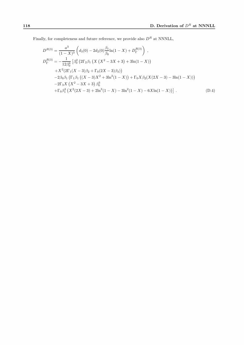
118 D. Derivation of DR at NNNLL
Finally, for completeness and future reference, we provide also DR at NNNLL,
DR(3) =a3
(1 −X)3
(
d3(0) − 2d2(0)β1
β0ln(1 −X) +D
R(3)Γ
)
,
DR(3)Γ = − 1
12β40
[
β20
(
2Γ2β1
(
X(
X2 − 3X + 3)
+ 3ln(1 −X))
+X2(2Γ1(X − 3)β2 + Γ0(2X − 3)β3))
−2β0β1
(
Γ1β1
(
(X − 3)X2 + 3ln2(1 −X))
+ Γ0Xβ2(X(2X − 3) − 3ln(1 −X)))
−2Γ3X(
X2 − 3X + 3)
β30
+Γ0β31
(
X2(2X − 3) + 2ln3(1 −X) − 3ln2(1 −X) − 6X ln(1 −X))]
. (D.4)
Summary
Introduction and Goals
There are four known fundamental interactions in nature: gravitational, electromagnetic, weak and
strong interactions. The former one is well described by the General Relativity theory. The other three are
combined into the Standard Model (SM), a relativistic quantum field theory built with the guidance of gauge
invariance and renormalizability. It is given in terms of a Lagrangian of quantized fields that describe the
elementary degrees of freedom, quarks and leptons, and the carriers of the interactions, the bosons. The SM
is divided in two sectors: the electroweak sector, which unifies the electromagnetic and weak interactions,
and the strong sector, described by Quantum Chromodynamics (QCD).
Understanding QCD has been pursued over for almost four decades from different perspectives: pertur-
bative QCD, lattice QCD, effective field theories (chiral perturbation theory, heavy-quark effective theory,
soft-collinear effective theory, etc), and other frameworks as well. Despite many efforts, the question of how
the observed properties of hadrons are generated by the dynamics of their constituents, namely quarks and
gluons, is yet to be resolved. A research venue that would be of much help, and which is being actively pur-
sued both theoretically and experimentally, is to try to explore the three-dimensional structure of nucleons,
both in momentum and configuration space. The role of quarks and gluons in generating the nucleon’s spin
or the partonic angular momentum is being investigated in experimental facilities such as JLab and DESY
and by HERMES, COMPASS or Belle collaborations, among others. The LHC, the most powerful hadron
collider we have nowadays, can also be of very much help in understanding the role of gluons inside the
protons. As mentioned before the ultimate goal is to try to understand how the dynamics of QCD generates
the observed features of hadrons in general and of nucleons in particular.
Among the different physical observables we can deal with, the ones with non-vanishing (or un-
integrated) transverse-momentum dependence are specially important at hadron colliders, and can be very
useful to understand the inner structure of hadrons. Moreover, those observables are relevant for the Higgs
boson searches and also for proper interpretation of signals of physics “beyond the Standard Model”. The
interest in such observables goes back to the first decade immediately after establishing QCD as the funda-
mental theory of strong interactions [1–5]. Recently, however, there has been a much renewed interest in
qT -differential cross sections where hadrons are involved either in the initial states or in the final ones or in
both (see e.g. [6–13]). The main issues of interest range from obtaining an appropriate factorization theorem
for a given process and resumming large logarithmic corrections to performing phenomenological analyses
and predictions.
In order to study the spin and momentum distributions of partons inside the nucleons, it has been
realized that one needs to identify an “irreducible” number of functions (or hadronic matrix elements). In
the collinear limit there are (at leading twist) three parton distribution functions (PDFs), depending on the
polarization of the partons: the momentum distribution [4, 5], the helicity distribution and the transversity
distribution [14]. When the intrinsic partons’ transverse momentum is also considered then one obtains, at
leading twist, eight transverse momentum dependent PDFs (TMDPDFs) 1 that characterize the nucleon’s
internal structure [15,16]. To be of any use, those matrix elements have to be properly defined at the operator
level (in terms of QCD degrees of freedom) and then their properties (such as evolution or universality) should
be carefully examined. Among that group of functions, the unpolarized TMDPDF has a special role. It
has no spin dependence, and thus it is considered as a “simple” generalization of the standard (integrated)
Feynman PDF. However since the introduction of this quantity by Collins and Soper thirty years ago and
despite many efforts [4–6, 10, 17–20], there has not been any agreed-upon definition of it. This fact clearly
has its bearings over the other, and more complicated, hadronic matrix elements as well, and it affects the
whole field of spin physics.
1Throughout this thesis we indistinctly use “TMD” for “transverse-momentum dependent” or “transverse-momentum distri-bution” (which refers both to transverse-momentum dependent parton distribution functions and transverse-momentumdependent fragmentation functions)
120 Summary
The integrated or collinear PDF is defined as
fq/P (x) =1
2
∫
dr−
2πe
12
ixP +r− 〈PS|ψ(0+, r−,~0⊥)W [r−; 0−]γ+
2ψ(0) |PS〉 ,
where the gauge link W [r−; 0−] connects the two points along the light-cone direction and preserves gauge
invariance (in chapters 1 and 2 it will be more clear the particular form of gauge links). From a probabilistic
point of view, this correlation function gives the number of partons (quarks) inside the nucleon that carry
a fraction x of the collinear momentum P+ of the parent nucleon. This matrix element is a fundamental
block of many factorization theorems. For instance, it appears in the factorization of the structure functions
of DIS [21]. The factorization theorems express a given observable in terms of perturbatively calculable
coefficients and non-perturbative hadronic matrix elements. The formers contain the information of short-
distance physics and do not contain any divergence. The hadronic matrix elements characterize the long-
distance physics of QCD and do have divergences when are calculated perturbatively.
Deriving a factorization theorem for a given hard process is in general a complicated task, and even
more harder it is to prove that it holds to all orders in perturbation theory. As already mentioned, a factor-
ization theorem is the mathematical statement that we can separate the perturbative and non-perturbative
contributions for a given observable, say a cross-section. And in order to be able to formulate it, one needs
to identify first which are the relevant scales and modes that contribute to a given process, and then assign
different matrix elements to them. Moreover, it is easy to imagine that one will find large logarithms of the
ratios of the scales in the perturbative calculations, and thus resummation will play a crucial role in order
to get any sensible results from the established factorization theorems.
In order to understand the meaning of a factorization theorem, let us consider the inclusive Drell-Yan
lepton pair production, hA(P )+hB(P ) → l1(k1)+l2(k2)+X(PX), where hA(B) are the two incoming hadrons,
l1(2) the outgoing leptons and X stands for unobserved hadrons in the final state. In this process we measure
the invariant mass of the outgoing lepton pair, M2 = q2 = (k1 + k2)2, and its rapidity, y = 12 ln q·P
q·P . The
factorization theorem for this process reads [22]
dσ
dM2dy=∑
i,j
∫ 1
xA
dxn
∫ 1
xB
dxn H
(
M2
µ2,xA
xn,xB
xn
)
fi/hA(xn;µ) fj/hB
(xn;µ) ,
where xA = ey√
M2/s, xB = e−y√
M2/s and s = (P + P )2 is the center of mass energy squared. This
theorem is correct up to power corrections suppressed by a power of M2. On one hand we have the hard part
H , which depends on M2 and does not have any divergence. On the other hand we have the two integrated
PDFs corresponding to the incoming hadrons.
If we perform a perturbative calculation of the PDF, it will contain an ultraviolet (UV) and an infra-red
(IR) divergence (see e.g. [21]). The UV one is removed by standard renormalization procedure, and it gives
us the evolution properties of the PDF (DGLAP splitting kernels). On the other hand, the IR divergence
is a direct manifestation of the non-perturbative character of the PDF, and is washed out by confinement
when plugged into a given factorization theorem. In particular, using pure dimensional regularization the
PDF at O(αs) is
fq/P (x) = δ(1 − x) +
(
1
εUV− 1
εIR
)
Pq←q ,
where Pq←q is the one-loop splitting kernel of a quark into a quark (see eq. (3.34)). This result is the
prototype of a perturbative calculation of a well-defined hadronic matrix element, where the UV and IR
divergencies are separated, i.e., which can be properly renormalized.
The hard part in the factorization theorem is calculated order by order in perturbation theory by
the “subtraction” method, i.e., by subtracting the combination of the two PDFs on the right hand side
to the cross-section dσ on the left hand side. Thus, it is a must that the hadronic matrix elements on
the right reproduce the IR contribution of the observable on the left, so that the subtraction gives us a
perturbative coefficient free from any divergence. From a practical point of view, we clearly need to perform
Summary 121
the perturbative calculation of dσ and the two PDFs in a consistent way, using the same IR regulator (pure
dimensional regularization, masses, offshellnesses, etc).
Regarding the hadronic matrix elements, their perturbative calculation could seem meaningless, in the
sense that it contains IR divergences. However it allows us to extract the perturbative hard part of the
factorization theorem by the subtraction method. The IR divergences have a clear non-perturbative origin
and are washed out by confinement. In a phenomenological application of the factorization theorem, the
PDFs (and any hadronic matrix element in general) are replaced by numerical functions extracted from the
experiment. Thus, the predictive power of pQCD lies on the universality of the relevant hadronic matrix
elements, which can be extracted from one hard reaction and used to make predictions for another reaction.
With the introduction of Soft-Collinear effective theory (SCET) [23–34] the derivation of factorization
theorems and the resummation of large logarithms has been largely simplified. From the effective theory point
of view one can understand a factorization theorem as a multistep matching procedure. Once the relevant
scales are identified, one needs to perform at each scale a matching between two effective theories, which have
to share the same IR physics. From each matching one will get a perturbative (Wilson) coefficient. At the
end, one will end up with different perturbative coefficients and non-perturbative hadronic matrix elements.
The resummation of large logarithms is done by running the coefficients and/or the matrix elements between
the relevant scales, using the Renormalization Group (RG) equations.
The success of SCET, though, is based on the fact that the relevant modes that reproduce the IR
physics of full QCD are collinear and soft. This is not true in general, and has to be proven (or at least
shown perturbatively and justified to all orders in perturbation theory) for any given process. It lies outside
of the scope of this thesis to analyze the issue related to the appearance of other modes, such as Glauber
modes, and the breakdown of SCET. For the processes we deal with, it is generally believed that collinear
and soft modes do reproduce the IR of QCD, and thus the use of SCET is justified [20, 21, 35]. Moreover,
we have checked this fact explicitly by performing O(αs) calculations.
Focusing back our attention on the transverse momentum of partons, we could think of generalizing
the factorization theorem given previously to the case where we not only measure the invariant mass of the
lepton pair, but also its transverse momentum. In this case, we could schematically write
dσ
dM2dq2⊥dy
=∑
i,j
∫ 1
xA
dxn
∫ 1
xB
dxn
∫
d2kn⊥d2kn⊥δ
(2)(q⊥ − kn⊥ − kn⊥)
×H
(
M2
µ2,xA
xn,xB
xn
)
Fi/hA(xn, kn⊥;µ)Fj/hB
(xn, kn⊥;µ) ,
where the TMDPDFs would be the generalization of the collinear PDFs,
Fq/P (x, k⊥) =1
2
∫
dr−d2r⊥(2π)3
e12
ixP +r−−i~k⊥·~r⊥
× 〈PS|ψ(0+, r−, ~r⊥)W [r−; 0−]W [~r⊥;~0⊥]γ+
2ψ(0) |PS〉 .
Notice that we have added a gauge link to connect the points also in the transverse direction. However, if we
perform a perturbative calculation of this quantity we will get rapidity divergences (RDs) and mixed UV/IR
divergences. Thus, this matrix element cannot be renormalized by any means, and it cannot be considered
as a valid hadronic matrix element.
In this thesis, by considering a process which is sensitive to the transverse-momentum of partons inside
the hadrons, and using the effective field theory machinery, we provide a proper definition of TMD hadronic
matrix elements. From their definition and based on the relevant factorization theorem, we obtain their
properties, mainly their evolution, which is of much importance for phenomenological applications and the
whole topic of spin-physics. Thus, three decades after the introduction of the collinear PDF, we complete
the puzzle by providing a proper theoretical definition of the functions that encode the 3-dimensional inner
structure of hadrons: TMDs.
Results
122 Summary
Soft-Collinear effective theory was formulated in covariant gauges, and it has proven to be a very
useful tool to derive factorization theorems for different processes and perform the resummation of large
logarithms in a cleaner and efficient way. However, for processes where the relevant matrix elements contain
a separation in the transverse direction, as the ones that the TMDs involve, SCET fails to provide a gauge
invariant definition for them. In chapter 2 we have explained the origin of transverse gauge links T within
SCET and studied which light-cone conditions are compatible with the power counting of the effective theory,
in such a way that the extended theory incorporates them right from the start, and all quantities built with
this theory are, for the first time, gauge invariant by definition [60]. The relevance of the T -Wilson lines in
SCET has been shown explicitly with the calculation at O(αs) of the Quark Form Factor and the TMDPDF
in Feynman and light-cone gauges.
In chapter 3 we have studied the Drell-Yan lepton pair production at small transverse momentum qT .
The analysis was carried out through the framework of the effective field theory via a two-step matching
procedure: QCD → SCET-qT → SCET-II. We established an all-order factorization theorem which allows
for a phenomenological study of DY qT spectrum to be analyzed at energies much larger than ΛQCD. When
considering the double-counting issue of the soft and the naive collinear regions properly, the obtained
factorization theorem serves as a guideline towards how the TMDPDF should be defined and what would be
its fundamental properties. In our calculations we have used Wilson lines defined on-the-light-cone and light-
cone singularities appearing in individual Feynman diagrams have been regularized with the ∆-regulator.
The fact that all Wilson lines are defined on-the-light-cone only facilitates this computation.
The two step factorization is necessary to perform the resummation of logs of qT /Q and ΛQCD/qT
respectively and we have discussed the resummation procedure in impact parameter space. In the first step
of the factorization one gets the usual structure of the cross section given in eq. (3.1). However the matrix
elements so defined are not good objects for the second factorization, because of the presence of mixed
UV/IR and rapidity divergences. All these divergences however disappear in the TMDPDF as we have
defined it. The second factorization is built up by matching the TMDPDF onto the PDF for large qT . We
have studied the Wilson coefficients that appear in the second matching which contain, in impact parameters
space, ln(Q2/µ2). We have shown that this kind of logs can be exponentiated, and thus resummed.
We have provided a definition of TMDPDFs which is gauge invariant and free from all rapidity diver-
gences including the mixed terms that spoil the renormalization of such quantities. The factorization theorem
for DY qT dependent spectrum, which is the basis leading towards defining a “TMDPDF”, is strongly be-
lieved to hold to all orders in perturbation theory and that the Glauber region is harmless. Since full QCD
quantities (like DY hadronic tensor) are free from RDs, then given the analysis presented in this work, one
can easily conclude that the RDs cancellation in the TMDPDF holds to all orders in perturbation theory.
This is important for phenomenological applications of TMDs (quarks in the case of DY or SIDIS or gluon
TMDPDFs for LHC physics) since the anomalous dimensions and the Q2-resummation kernel D [37], and
thus the evolution of individual TMDs can now be properly determined [92]. Our results can be readily
extended to define polarized and unpolarized quark and gluon TMDPDFs which could be considered as a
generalization of the one introduced in [92], as well as TMDFFs as in chapter 5.
We have also shown, by generalizing the arguments given in [67], how the TMDPDF definition, which
can be referred to as the “modified EIS” definition, is equivalent to the JCC one in the sense that both
definitions manage to cancel rapidity divergences in bi-local quark field operators separated along one light-
cone direction and also in the transverse two-dimensional space. Our definition can be readily used to carry
out perturbative calculations beyond O(αs) (with any convenient regulator, the ∆-regulator or any other
one) and calculate explicitly, for example, the anomalous dimension of polarized (such as Sivers function)
and unpolarized TMDs.
The inclusion of the square root of the soft function in the definition of the TMDPDF has important
consequences. First of all, the double counting in the factorization theorem is taken into account. Second, it
allows for the separation of UV and IR divergences in the TMDPDF. And third, even with the subtraction
of the square root of the soft function we are able to recover the PDF from the TMDPDF by integrating
over the transverse momentum.
In chapter 5 we also considered the TMDPDF with DIS kinematics and pointed out the differences
with respect to DY ones. As mentioned earlier, different Wilson lines are needed for the two kinematical
Summary 123
settings. However we established the universality of the TMDPDF in both regimes and argued its validity
to all orders in perturbation theory. In that chapter we followed the same steps as in chapter 3 in order to
obtain the factorization theorem for SIDIS and define the TMDFF, similarly to the TMDPDF. We performed
a complete one-loop calculation and showed the refactorization of this quantity in terms of the collinear FF,
being able to discuss the former’s evolution properties.
We have argued in chapter 4 that the evolution of leading twist TMDPDFs, both for polarized and
unpolarized ones, is driven by the same kernel [92], which can be obtained up to NNLL accuracy by using
the currently known results for the cusp anomalous dimension and the QCD β-function. For completeness,
we have provided as well an expression for the evolution kernel at NNNLL. As shown in chapter 5, this kernel
applies as well to all leading twist TMDFFs.
The evolution kernel, as a function of the impact parameter b, can be obtained in the perturbative
region without introducing any model dependence, and the resummation can be performed up to any desired
logarithmic accuracy. This resummation can be done either by solving a recursive differential equation or
by properly implementing the running of the strong coupling with renormalization scale within the standard
CSS approach. In both cases we obtained identical results. This fact is actually not surprising. The
definition of (unpolarized) TMDPDF, both in the EIS [75] and JCC [20] approaches has been shown to be
equivalent [67, 75]. If the resummation of the large logarithms is performed properly and consistently (in
terms of logarithmic accuracy) then the final results for the evolved TMDs should agree as well. We consider
this agreement as one of the major contributions of this work as it unifies a seemingly different approaches
to TMD theory and phenomenology.
As already mentioned, one of the main contributions is to give a parameter free expression for the
evolution kernel by using the highest order perturbatively calculable known ingredients, which is valid only
within the perturbative domain in the impact parameter space. On the other side, within the CSS approach
there is an overlap between the perturbative and non-perturbative contributions to the evolution kernel,
due to the implementation of a smooth cutoff through the b∗ prescription. Comparing both approaches,
we conclude that bmax = 1.5 GeV−1, which is more consistent with our results (see fig. 4.4), gives a better
description of the perturbative region within the CSS approach, as was actually found by phenomenological
fits in [77].
We have studied under which kinematical conditions the non-perturbative contribution to the kernel
is negligible, and hence our approximate expression for the kernel (in Eq. (4.22)) can be applied without
recurring to any model for all practical purposes. Given an initial scale Qi =√
2.4 GeV, at which one
would like to extract the low energy models for TMDs, if the final scale is Qf ≥ 5 GeV, then the effects of
non-perturbative physics are washed out, as is shown in Fig. 4.2. In this case, all the model dependence is
restricted to the low energy functional form of TMDs to be extracted by fitting to data.
Thus, phenomenologically, the major point of our work is to provide a scheme optimized for the
extraction of TMDs from data. Assuming that low energy models are to be extracted at scale Qi ∼ 1−2 GeV,
if data are selected with Qf > 5 GeV, then the evolution is in practice parameter free. For instance,
COMPASS, Belle or BaBar facilities can perfectly fulfill these requirements.

ResumenIntroducción y Objetivos
Se conocen cuatro fuerzas fundamentales en la Naturaleza: la gravitacional, la electromagnética, la
nuclear débil y la nuclear fuerte. La primera estś descrita por la Teoría General de la Relatividad. Las
otras tres se combinan en el Modelo Estándar (SM), una teoría cuántica de campos relativista construida
siguiendo los principios de la invariancia gauge y la renormalizabilidad. Está dada en thermanos de un
Lagrangiano de campos cuantizados que describen los grados de libertad elementales, quarks y letones, y los
portadores de las interacciones, los bosones. El SM está dividido en dos sectores: el electrodédil, que unifica
las interacciones electromagnética y nuclear dédil, y el sector fuerte, que está descrito por la Cromodinámica
Cuántica (QCD).
Durante las últimas cuatro déchadas se ha intentado entender la teoría de QCD desde diferentes
perspectivas: QCD perturbativa, QCD en el retículo, teorías efectivas (teoría quiral perturbativa, teoría
efectiva de quarks pesados, teoría efectiva soft-collinear, etc), y otras. A pesar de los numerosos esfuerzos,
la cuestión de cómo las propiedades observadas de los hadrones se originan a partir de la dinmica de sus
constituyentes sigue sin estar resuelta. Una posible vía de investigación que podría ser de gran ayuda, y que
está siendo llevada a cabo muy activamente tanto teóricamente como experimentalmente, es intentar explorar
la estructura tridimensional de los nucleones, tanto en el espacio de momentos como en el de configuración.
El rol de los quarks y gluones en la generación del espín de los nucleones o la composición del momento
angular partónico está siendo investigado en experimentos y laboratorios como JLab, DESY, HERMES,
COMPASS o Belle, entre otros. El LHC, el colisionador de hadrones más potente jamás construido, puede
ser también de mucha utilidad para averiguar el rol de los gluones dentro de los protones. Tal y como se
dijo anteriormente, el objetivo final es el comprender cómo la dinámica de QCD genera las propiedades
observadas de los hadrones en general, y de los nucleones en particular.
Entre los diferentes observables que podemos tratar, son especialmente importantes en los colisionadores
de hadrones aquéllos que tienen un momento transverso no nulo. Además estos observables son útiles para
la búsqueda de Higgs y para una adecuada interpretación de señales de nueva física más allá del Modelo
Estándar. El interés por este tipo de observablas se remonta a la primera década después de que QCD se
estableciera como la teoría fundamental de las interacciones fuertes [1–5]. Sin embargo, recientemente ha
aparecido un renovado interés por las secciones eficaces diferenciales en el qT , ya sea con hadrones en el
estado inicial, final o en ambos (ver e.g. [6–13]). Las cuestiones de mayor interés van desde la obtención de
los teoremas de factorización adecuados para los procesos considerados y la resumación de logaritmos, hasta
la realización de análisis fenomenológicos.
Para poder estudiar las distribuciones de espín y momento de los partones dentro de los nucleones
es necesario manejar un nmuero “irreducible” de funciones (o elementos de matriz hadrónicos). En el
límite colineal, al “leading twist”, tenemos tres funciones de distribución de patrones (PDFs), dependiendo
de la polarización de los partones: la distribución de momento [4, 5], la distribución de helicidad y la
distribution de transversidad [14]. Cuando consideramos también el momento transverso de los partones,
obtenemos, de nuevo al “leading twist”, ocho distribuciones de partones de momento transverso (TMDPDFs)
que caracterizan la estructura interna de los nucleones [15, 16]. Para ser de alguna utilidad, estos elemento
de matriz deben estar correctamente definidos al nivel de operadores (en términos de los grados de libertad
de QCD) y sus propiedades (como la evolución o la universalidad) adecuadamente examinadas. De estas
ocho distribuciones, la TMDPDF no polarizada tiene un rol especial. No depende del espín, y por tanto la
podemos considerar como una “simple” generalización de la PDF estándar (o integrada) de Feynman. Sin
embargo, a pesar de los múltiples esfuerzos desde que esta cantidad fue propuesta por Collins y Soper hace
treinta años [4–6, 10, 17–20], no se ha obtener una definión consensuada por la comunidad. Además, este
hecho se extiende al resto de las funciones, que son más complicadas, y afecta al campo de la física de espín
en general.
La PDF integrada o colineal se define como
fq/P (x) =1
2
∫
dr−
2πe
12
ixP +r− 〈PS|ψ(0+, r−,~0⊥)W [r−; 0−]γ+
2ψ(0) |PS〉 ,
126 Resumen
donde el “gauge link” W [r−; 0−] conecta los dos puntos en la dirección del cono de luz y garantiza la
invariancia gauge (en los capítulos 1 y 2 se aclarará la forma funcional y el rol de estos “gauge links”). Desde
el punto de vista probabilístico, esta función de correlación nos da el número de partones (quarks) destro
del nucleón que tiene una francción x del momento colineal P+ del nucleón. Este elemento de matriz es
una pieza fundamental en muchos teoremas de factorización. Por ejemplo, aparece en la factorización de las
funciones de estructura de DIS [21]. Los teoremas de factorización exoresan un observable dado en función de
coeficientes calculables perturbativamente y elementos de matriz no perturbativos. Los primeros contienen
información sobre la física de cortas distancias y no contienen ninguna divergencia. Los elementos de matriz
hadrónicos caracterizan la física de largas distancias de QCD y sí contienen divergencias cuando se calculan
perturbativamente.
Derivar el teorema de factorización de un proceso dado es en general una ardua tarea, y más el conseguir
probar que es correcto a todos los órdenes en teoría de perturbaciones. Tal y como se dijo antes, un
teorema de factorización es la formulación matemática del hecho de que podemos separar las contribuciones
perturbativa y no perturbativa para un observabe dado, por ejemplo una sección eficaz. Y para ser capaces
de llegar a formularlo, necesitamos primero identificar las escalas y modos relevantes que contribuyen al ese
proceso, y después asignarles operadores. Además, es fácil imaginar que al hacer cálculos perturbativos nos
encontraremos con grandes logaritmos de los cocientes de las escalas relevantes, y por tanto la resumación
jugará un papel crucial a la hora de extraer cualquier conclusión a partir de los teoremas de factorizción
establecidos.
Para entender un poco mejor el significado de un teorema de factorización, consideremos la produción
inclusiva de letones de Drell-Yan, hA(P ) + hB(P ) → l1(k1) + l2(k2) + X(PX), donde hA(B) son los dos
hadrones que comisionan, l1(2) los letones producidos y X los hadrones no observados en el estado final. En
este proceso medimos la masa invariante del par de leptones, M2 = q2 = (k1 +k2)2, y su rapidity, y = 12 ln q·P
q·P .
El teorema de factorización para este proceso es [22]
dσ
dM2dy=∑
i,j
∫ 1
xA
dxn
∫ 1
xB
dxn H
(
M2
µ2,xA
xn,xB
xn
)
fi/hA(xn;µ) fj/hB
(xn;µ) ,
donde xA = ey√
M2/s, xB = e−y√
M2/s y s = (P + P )2 es la energía del centro de masa al cuadrado. Es
teorema tiene correcciones suprimidas por potencias de M2. Por un lado tenemos la parte “hard” H , que
depende de M2 y no contiene ninguna divergencia. Por otro lado tenemos las dos PDFs, correspondientes a
los ladrones entrantes.
Si hacemos un cáculo perturbativo de la PDF, éste tendrá una divergencia ultravioleta (UV) y otra
infra-roja (IR) (ver e.g. [21]). La UV se elimina por el procedimiento estándar de renormalización, y nos
da las propiedades de evolución de la PDF (funciones de DGLAP). Por otro lado, la divergencia IR es una
manifestación directa de la naturaleza no perturbative de la PDF, y es absorbida por el confinamiento cuando
la insertamos en un teorema de factorización. En particular, utilizando regularización dimensional pura, la
PDF al O(αs) es
fq/P (x) = δ(1 − x) +
(
1
εUV− 1
εIR
)
Pq←q ,
donde Pq←q es el “splitting kernel” a un loop de un quark en un quark (ver eq. (3.34)). Este resultado es el
prototipo de un cáculo perturbativo de un elemento de matriz hadrónico bien definido, donde las divergencias
UV e IR están separadas y por tanto es posible su renormalización.
La parte “hard” en el teorema de factorización se calcula orden a orden en teoría de perturbaciones
por el método de la substracción, i.e., substrayendo la combinación de las dos PDFs a a la sección eficaz
dσ. Por tanto, es necesario que los elementos de matriz hadrónicos en el miembro de la derecha del teorema
reproduzcan las divergencias IR del observable que factorizamos, de tal forma que al substraerlos obtengamos
un coeficiente perturbativo sin divergencias. Desde un punto de vista más práctivo, esto requiere que los
cálculos perturbativos de las dos PDFs y la sección eficaz se hagan de manera consistente, es decir, que
utilicemos el mismo regulador para las divergencias IR (regularización dimensional, masas, “offshellnesses”,
Resumen 127
etc).
Respecto a los elementos de matriz hadrónicos, su cálculo perturbativo podría parecer inútil, ya que
contiene divergencias IR. Sin embargo, nos permite extraer la parte “hard” a partir del teorema de factor-
ización por el método de la substracción. Las divergencias IR tienen un origen puramente no perturbativo y
son absorbidas por el confinamiento. En la aplicación fenomenológica del teorema de factorización, las PDFs
(y cualquier elemento de matriz hadrónico en general) son reemplazados por funciones numé ricas extraídas
previamente de los datos experimentales. Por tanto, el poder predictivo de pQCD se basa en la universalidad
de los elementos de matriz hadrónicos relevantes, que se pueden obtener en un cierto proceso y utilizados
para hacer predicciones para otro proceso diferente.
Con la introducción de la teoría efectiva “Soft-Collinear” (SCET) [23–34], la derivación de teoremas de
factorizaciń y la esumación de logaritmos se ha simplificado enormemente. Desde el punto de vista de teorías
efectivas podemos entender un teorema de factorización como un proceso de empalmes consecutivos. Una
vez que las escalas relevantes están identificadas, tenemos que empalmar en cada una de ellas dos teorías
efectivas, una por arriba y otra por abajo, que comparten la misma física IR. De cada empalme obtenemos
un coeficiente perturbativo (de Wilson). Al final, tendremos un conjunto de coeficientes, tantos como escalas,
y elementos de matriz no perturbativos que nos darán la contribución IR. La resumación de logaritmos se
lleva a cabo tomando los coeficientes y elementos de matriz y evolucionándolos entre las escalas relevantes,
utilizando las ecuaciones del Grupo de Renormalización.
El éxito de SCET, sin embargo, está basado en la asunción de que los modos que reproducen la física IR
de QCD son los colineales y soft. Esto no es cierto en general, y debe ser probado para cada caso, o al menos
refrendado con cálculos perturbativos y argumento a todos los órdenes. No entra dentro de los objetivos
de esta tesis el analizar esta cuestión, relacionada con la necesidad de otros modos, como los Glaubers, y
la consecuente limitación de SCET (ver e.g. [59]). Para los procesos que consideramos, está ampliamente
aceptado que los modos colineales y soft sí reproducen la física IR de QCD, y por tanto el uso de SCET está
justificado [20, 21, 35]. Además hemos comprobado este hecho explícitamente para cada caso a O(αs).
Centrándonos de nuevo sobre el momento transverso de los partones, podríamos pensar en generalizar
el teorema de factorización dado previamente al caso en el que no sólo medimos la masa invariante del par
de leptones, sino también su momento transverso. En este caso, podríamos escribir esquemáticamente
dσ
dM2dq2⊥dy
=∑
i,j
∫ 1
xA
dxn
∫ 1
xB
dxn
∫
d2kn⊥d2kn⊥δ
(2)(q⊥ − kn⊥ − kn⊥)
×H
(
M2
µ2,xA
xn,xB
xn
)
Fi/hA(xn, kn⊥;µ)Fj/hB
(xn, kn⊥;µ) ,
donde las TMDPDFs serían la generalización de las PDFs colineales,
Fq/P (x, k⊥) =1
2
∫
dr−d2r⊥(2π)3
e12
ixP +r−−i~k⊥·~r⊥
× 〈PS|ψ(0+, r−, ~r⊥)W [r−; 0−]W [~r⊥;~0⊥]γ+
2ψ(0) |PS〉 .
Notar que hemos añadido otro “gauge link” para conectar los puntos también en la dirección transversa.
Sin embargo, si hacemos un cáculo perturbativo de esta función obtendremos divergencias de rapidity y
divergencias mixtas UV/IR. Por tanto, este elemento de matriz no puede renormalizarse, y en ningún caso
entonces puede ser considerado como un elemento de matriz hadrónico válido.
En esta tesis, considerando procesos sensibles al momento transverso de los partones, y utilizando
la maquinaria de teorás efectivas (en particular SCET), obtenemos la definicón correcta de las TMDs. A
partir de su definición y basándinos en los teoremas de factorización relevantes, analizamos sus propiedades,
principalmente su evolución, que es de vital importancia para aplicaciones fenomenológicas y el campo de la
física de espín. En conclusión, tres décadas después de que la PDF colineal fuera propuesta, completamos
el puzle dando una correcta definición teórica de las funciones que describen la estructura tridimensional
interna de los hadrones: las TMDs.
128 Resumen
Resultados
SCET fue formulada para gauges covariantes, y se ha mostrado una herramienta muy útil para derivar
teoremas de factorización para diferentes procesos y efectuar la correspondiente resumación de grandes
logaritmos de una forma eficiente. Sin embargo, para procesos en los que los elementos de matriz relevantes
contienen una separación en la dirección transversa, como los que forman parte de las TMDs, SCET no es
capaz de dar para ellos una definición invariante gauge. En el capítulo 2 hemos explicado el origen de las
líndas de Wilson transversas T dentro de SCET, y además hemos estudiado qué condiciones del cono de
luz son compatibles con el contaje de potencias de esta teoría. Así, hemos extendido la teoría de tal forma
que estas líneas aparecen desde el principio y, por primera vez, todas las cantidades definidas con SCET
son invariantes gauge desde el principio [60]. Hemos mostrado explícitamente la relevancia de las líneas
de Wilson T en SCET calculando a O(αs) el Factor de Forma de Quarks y la TMDPDF en los gauges de
Feynman y el cono de luz.
En el captitulo 3 hemos estudiado el espectro de momento transverso qT de producción Drell-Yan
de un par de leptones. El análisis se ha hecho dentro del marco de las teotrías efectivas, realizando un
procedimiento de empalme en dos pasos: QCD → SCET-qT → SCET-II. Hemos establecido el teorema de
factorización a todos los órdenes, que permite realizar estudios fenomenológicos del espectro de qT de DY a
energías mucho más altas que ΛQCD. Al considerar el problema del doble contaje entre las regiones colineales
y soft, el teorema de factorización obtenido sirve como guía para poder definir correctamente las TMDPDFs,
así como para analizar sus propiedades fundamentales. En los cálculos hemos utilizado las líneas de Wilson
definidas en el cono de luz, y las singularidades de rapidity que aparecen en los diferentes diagramas de
Feynman las hemos regularizado utilizando el regulador ∆.
La factorización en dos pasos es necesaria para realizar la resumación de logaritmos de qT /Q y ΛQCD/qT
respectivamente, que además hemos hecho en el espacio del parámero de impacto. En el primer paso de la
factorización obtenemos la estructura habitual de la sección eficaz dada en la eq. (3.1). Pero los elementos de
matriz que aparecen en esa fórmula no están bien definidos y no sirven para realizar la segunda factorización,
ya que contienen divergencias de rapidity. Estas divergencias, por el contrario, desaparecen en la TMDPDF
tal y como la hemos definido. La refactorización se realiza empalmando la TMDPDF con la PDF para qT
grande. Hemos analizado los coeficientes de Wilson que aparecen en la segunda factorización, que contienen
logaritmos ln(Q2/µ2) en el espacio del parámetro de impacto, y que pueden ser exponenciados y por tanto
rezumados.
Hemos dado una definición de las TMDPDFs que es invariante gauge y que no posee divergencias de
rapidity que puedan destruir su renormalizabilidad. El teorema de factorización del espectro de qT de DY, que
es la base sobre la que nos apoyamos para definir las TMDPDFs, se cree firmemente que es correcto a todos
los órdenes en teoría de perturbaciones, y que las región de Glauber es irrelevante. Como cualquier cantidad
en QCD (como el tensor hadrónico) no posee divergencias de rapidity, entonces dada la consistencia del
teorema de factorización presentado en este trabajo podemos concluir que la cancelación de las divergencias
de rapidity en las TMDPDFs definidas se da a todos los órdenes en teoría de perturbaciones. Este hecho
es importante para la fenomenología de TMDs en general, ya que la dimensión anómala y la resumación
del Q2 en la función D [37], y por tanto la evolución de cada TMD individualmente está adecuadamente
determinada [92]. Los resultados de esta tesis se pueden extender fácilmente a la definición de TMDPDFs
polarizadas y no polarizadas, tanto de quarks como de gluones, así como a las TMDFFs tal y como se explica
en el capítulo 5.
Generalizando los argumentos de [67] hemos mostrado cómo la definición de la TMDPDF dada (“EIS
modificada”) es equivalente a la de JCC, en el sentido de que ambas están libres de divergencias de rapidity
en operadores bi-locales de quarks con separación en la dirección del cono de luz y en la transversa. Nuestra
definición es útil para realizar cálculos más allá del O(αs) (con cualquier regulador conveniente, ya sea el
regulador ∆ u otro) y obtener explícitamente, por ejemplo, la dimensión anómala de TMDs polarizadas
(como la función de Sivers, Boer-Mulders o Collins) y no polarizadas.
La inclusión de la raíz de la función soft en la definición de las TMDPDF tiene importantes consecuen-
cias. Por un lado, se tiene en cuenta el problema del doble contaje en el teorema de factorización. Por otro,
permite la separación de divergencias UV e IR y la cancelación de divergencias de rapidity. Y finalmente,
Resumen 129
incluso con la función soft en la definción de la TMDPDF, somos capaces de recuperar la PDF colineal
integrando la TMDPDF en el momento transverso.
En el captitulo 5 hemos considerado también la TMDPDF con la cinemática de DIS, mostrando las
diferencias con respecto a la de DY. Tal y como se explicó, son necesarias diferentes líndas de Wilson para
estos dos procesos. Sin embargo, hemos establecido explícitamente a O(αs) la universalidad de la TMDPDF
no polarizada en ambos procesos y argumentado su validez a todos los órdenes en teoría de perturbaciones.
En este mismo capítulo hemos seguido los mismo pasos que en capítulo 3 para obtener el teorema de
factorización para SIDIS y definir la TMDFF, de manera análoga a la TMDPDF. Hemos realizado un cáculo
completo a O(αs) de la TMDFF y mostrado su refactorización en función de la FF colineal, obteniendo así
las propiedades de evolución de la TMDFF.
Hemos argumentado en el captitulo 4 que la evolución de las TMDPDFs al “leading twist”, tanto la
no polarizada como las polarizadas, está dada por el mismo evolutor [92], que puede obtenerse al NNLL
utilizando los resultados conocidos actualmente para la dimensión anóvala cusp y la función β de QCD. Por
completitud hemos proporcionado la expresión del evolutor al NNNLL para referencia futura. Tal y como
se explica en el capítulo 5, este evolutor se aplica también a las TMDFFs al “leading twist”.
El evolutor, como una función del parámero de impacto b, se puede obtener en la región perturbativa
sin necesidad de introducir ningún modelo, y la resumación se puede realizar hasta la precisión logarítmica
que se desee. Esta resumación se puede llevar a cabo tanto con la resolución de una ecuación diferencial
recursiva como con la evolución de la constante de acoplo fuerte en función de la escala de renormalización
(método de CSS). Ambas opciones dan idénticos resultados, tal y como es de esperar. De hecho, la definición
de la TMDPDF de JCC [20] y EIS [75] es equivalente [67, 75], y por tanto si la resumación de logaritmos
se hace de manera consistente (en términos de precisión logarítmica), debe ofrecer los mismos resultados
para las TMDs evolucionadas. Consideramos esta consistencia como una de las mayores contribuciones de
este trabajo, ya que unifica dos métodos aparentemente diferentes en cuanto a la teoría y fenomenología de
TMDs.
Tal y como hemos mencionado, uno de los puntos más importantes de este trabajo en cuanto a la
evolución de las TMDs es proporcionar una expresión libre de parámetros para su evolutor, utilizando
los ingredientes necesarios a la mayor precisión conocida actualmente. En el método de CSS existe un
solapamiento entre las contribuciones perturbativa y no perturbativa al evolutor, debido a que se implementa
un corte suave a través de la prescripción de b∗. Comparando su método con el nuestro (ver fig. 4.4),
concluimos que bmax = 1.5 GeV−1, porque ambos concuerdan en la región perturbativa. Esto fue observado
previamente en [77] realizando un análisis fenomenológico.
Hemos estudiado bajo qué condiciones la contribución no perturbativa al evolutor es despreciable, y
por tanto es aplicable nuestra expresión aproximada (en la eq. (4.22)) sin necesidad de recurrir a modelos
no perturbativos. Dada una escala inicial Qi =√
2.4 GeV a la que uno querría extraer los modelos de
bajas energías para las TMDs, si la escala final es Qf ≥ 5 GeV entonces los efectos no perturbativos no
juegan ningún papel, tal y como se muestra en la fig. 4.2. En este caso toda la dependencia del modelo está
restringida a la forma funcional de las TMDs a bajas energías que queremos obtener ajustando los datos
experimentales.
Por tanto, fenomenológicamente, la contribución más importante de nuestro trabajo es el proporcionar
un método optimizado para la extracción de las TMDs de los datos experimentales. Asumiendo que los
modelos a bajas energías de las TMDs se quieren extraer a Qi ∼ 1 − 2 GeV, si los datos se seleccionan con
Qf > 5 GeV entonces la evolución es totalmente perturbativa y no depende de ningún modelo. Por ejemplo,
COMPASS, Belle o BaBar pueden perfectamente cumplir con estas condiciones cinemaáticas.

Bibliography[1] G. Parisi and R. Petronzio, Small Transverse Momentum Distributions in Hard Processes, Nucl.Phys. B154 (1979) 427.
[2] G. Curci, M. Greco, and Y. Srivastava, QCD JETS FROM COHERENT STATES, Nucl.Phys. B159 (1979) 451.
[3] Y. L. Dokshitzer, D. Diakonov, and S. Troian, Hard Processes in Quantum Chromodynamics, Phys.Rept. 58 (1980)
269–395.
[4] J. C. Collins and D. E. Soper, Back-To-Back Jets in QCD, Nucl.Phys. B193 (1981) 381.
[5] J. C. Collins and D. E. Soper, Parton Distribution and Decay Functions, Nucl.Phys. B194 (1982) 445.
[6] S. Mantry and F. Petriello, Factorization and Resummation of Higgs Boson Differential Distributions in Soft-Collinear
Effective Theory, Phys.Rev. D81 (2010) 093007, [arXiv:0911.4135].
[7] S. Mantry and F. Petriello, Transverse Momentum Distributions in the Non-Perturbative Region, Phys.Rev. D84 (2011)
014030, [arXiv:1011.0757].
[8] T. Becher and M. Neubert, Drell-Yan production at small qT , transverse parton distributions and the collinear anomaly,
Eur.Phys.J. C71 (2011) 1665, [arXiv:1007.4005].
[9] T. Becher, M. Neubert, and D. Wilhelm, Electroweak Gauge-Boson Production at Small qT : Infrared Safety from the
Collinear Anomaly, JHEP 1202 (2012) 124, [arXiv:1109.6027].
[10] J.-Y. Chiu, A. Jain, D. Neill, and I. Z. Rothstein, A Formalism for the Systematic Treatment of Rapidity Logarithms in
Quantum Field Theory, JHEP 1205 (2012) 084, [arXiv:1202.0814].
[11] P. Sun, B.-W. Xiao, and F. Yuan, Gluon Distribution Functions and Higgs Boson Production at Moderate Transverse
Momentum, Phys.Rev. D84 (2011) 094005, [arXiv:1109.1354].
[12] S. M. Aybat, J. C. Collins, J.-W. Qiu, and T. C. Rogers, The QCD Evolution of the Sivers Function, Phys.Rev. D85
(2012) 034043, [arXiv:1110.6428].
[13] Z.-B. Kang, B.-W. Xiao, and F. Yuan, QCD Resummation for Single Spin Asymmetries, Phys.Rev.Lett. 107 (2011)
152002, [arXiv:1106.0266].
[14] J. P. Ralston and D. E. Soper, Production of Dimuons from High-Energy Polarized Proton Proton Collisions, Nucl.Phys.
B152 (1979) 109.
[15] P. Mulders and R. Tangerman, The Complete tree level result up to order 1/Q for polarized deep inelastic
leptoproduction, Nucl.Phys. B461 (1996) 197–237, [hep-ph/9510301].
[16] D. Boer and P. Mulders, Time reversal odd distribution functions in leptoproduction, Phys.Rev. D57 (1998) 5780–5786,
[hep-ph/9711485].
[17] X.-d. Ji, J.-p. Ma, and F. Yuan, QCD factorization for semi-inclusive deep-inelastic scattering at low transverse
momentum, Phys.Rev. D71 (2005) 034005, [hep-ph/0404183].
[18] X.-d. Ji, J.-P. Ma, and F. Yuan, QCD factorization for spin-dependent cross sections in DIS and Drell-Yan processes at
low transverse momentum, Phys.Lett. B597 (2004) 299–308, [hep-ph/0405085].
[19] I. Cherednikov and N. Stefanis, Wilson lines and transverse-momentum dependent parton distribution functions: A
Renormalization-group analysis, Nucl.Phys. B802 (2008) 146–179, [arXiv:0802.2821].
[20] J. Collins, Foundations of perturbative QCD. Cambridge monographs on particle physics, nuclear physics and cosmology.
32, 2011.
[21] G. F. Sterman, An Introduction to quantum field theory. 1994.
[22] J. C. Collins, D. E. Soper, and G. F. Sterman, Factorization of Hard Processes in QCD, Adv.Ser.Direct.High Energy
Phys. 5 (1988) 1–91, [hep-ph/0409313].
[23] C. W. Bauer, S. Fleming, and M. E. Luke, Summing Sudakov logarithms in B → Xsγ in effective field theory, Phys.Rev.
D63 (2000) 014006, [hep-ph/0005275].
[24] C. W. Bauer, S. Fleming, D. Pirjol, and I. W. Stewart, An Effective field theory for collinear and soft gluons: Heavy to
light decays, Phys.Rev. D63 (2001) 114020, [hep-ph/0011336].
[25] C. W. Bauer and I. W. Stewart, Invariant operators in collinear effective theory, Phys.Lett. B516 (2001) 134–142,
[hep-ph/0107001].
[26] C. W. Bauer, D. Pirjol, and I. W. Stewart, A Proof of factorization for B → Dπ, Phys.Rev.Lett. 87 (2001) 201806,
[hep-ph/0107002].
[27] C. W. Bauer, D. Pirjol, and I. W. Stewart, Soft collinear factorization in effective field theory, Phys.Rev. D65 (2002)
054022, [hep-ph/0109045].
[28] C. W. Bauer, D. Pirjol, and I. W. Stewart, Power counting in the soft collinear effective theory, Phys.Rev. D66 (2002)
054005, [hep-ph/0205289].
[29] A. V. Manohar, T. Mehen, D. Pirjol, and I. W. Stewart, Reparameterization invariance for collinear operators,
Phys.Lett. B539 (2002) 59–66, [hep-ph/0204229].
132 Bibliography
[30] M. Beneke, A. Chapovsky, M. Diehl, and T. Feldmann, Soft collinear effective theory and heavy to light currents beyond
leading power, Nucl.Phys. B643 (2002) 431–476, [hep-ph/0206152].
[31] C. W. Bauer, D. Pirjol, and I. W. Stewart, Factorization and endpoint singularities in heavy to light decays, Phys.Rev.
D67 (2003) 071502, [hep-ph/0211069].
[32] C. W. Bauer, S. Fleming, D. Pirjol, I. Z. Rothstein, and I. W. Stewart, Hard scattering factorization from effective field
theory, Phys.Rev. D66 (2002) 014017, [hep-ph/0202088].
[33] C. W. Bauer, D. Pirjol, and I. W. Stewart, On Power suppressed operators and gauge invariance in SCET, Phys.Rev.
D68 (2003) 034021, [hep-ph/0303156].
[34] A. V. Manohar and I. W. Stewart, The Zero-Bin and Mode Factorization in Quantum Field Theory, Phys.Rev. D76
(2007) 074002, [hep-ph/0605001].
[35] G. F. Sterman, Partons, factorization and resummation, TASI 95, hep-ph/9606312.
[36] C. Marcantonini and I. W. Stewart, Reparameterization Invariant Collinear Operators, Phys.Rev. D79 (2009) 065028,
[arXiv:0809.1093].
[37] M. G. Echevarria, A. Idilbi, and I. Scimemi, Factorization Theorem For Drell-Yan At Low qT And Transverse
Momentum Distributions On-The-Light-Cone, JHEP 1207 (2012) 002, [arXiv:1111.4996].
[38] J.-y. Chiu, A. Fuhrer, A. H. Hoang, R. Kelley, and A. V. Manohar, Soft-Collinear Factorization and Zero-Bin
Subtractions, Phys.Rev. D79 (2009) 053007, [arXiv:0901.1332].
[39] A. V. Manohar, Deep inelastic scattering as x → 1 using soft collinear effective theory, Phys.Rev. D68 (2003) 114019,
[hep-ph/0309176].
[40] A. Idilbi and I. Scimemi, Singular and Regular Gauges in Soft Collinear Effective Theory: The Introduction of the New
Wilson Line T, Phys.Lett. B695 (2011) 463–468, [arXiv:1009.2776].
[41] G. Ovanesyan and I. Vitev, An effective theory for jet propagation in dense QCD matter: jet broadening and
medium-induced bremsstrahlung, JHEP 1106 (2011) 080, [arXiv:1103.1074].
[42] I. W. Stewart, F. J. Tackmann, and W. J. Waalewijn, Factorization at the LHC: From PDFs to Initial State Jets,
Phys.Rev. D81 (2010) 094035, [arXiv:0910.0467].
[43] A. Bassetto, M. Dalbosco, I. Lazzizzera, and R. Soldati, Yang-Mills Theories in the Light Cone Gauge, Phys.Rev. D31
(1985) 2012.
[44] S. Mandelstam, Light Cone Superspace and the Ultraviolet Finiteness of the N=4 Model, Nucl.Phys. B213 (1983)
149–168.
[45] J. C. Collins and F. Hautmann, Soft gluons and gauge invariant subtractions in NLO parton shower Monte Carlo event
generators, JHEP 0103 (2001) 016, [hep-ph/0009286].
[46] J. C. Collins and F. Hautmann, Infrared divergences and nonlightlike eikonal lines in Sudakov processes, Phys.Lett.
B472 (2000) 129–134, [hep-ph/9908467].
[47] I. Cherednikov and N. Stefanis, Renormalization, Wilson lines, and transverse-momentum dependent parton distribution
functions, Phys.Rev. D77 (2008) 094001, [arXiv:0710.1955].
[48] F. D’Eramo, H. Liu, and K. Rajagopal, Transverse Momentum Broadening and the Jet Quenching Parameter, Redux,
Phys.Rev. D84 (2011) 065015, [arXiv:1006.1367].
[49] A. Idilbi and A. Majumder, Extending Soft-Collinear-Effective-Theory to describe hard jets in dense QCD media,
Phys.Rev. D80 (2009) 054022, [arXiv:0808.1087].
[50] J. C. Collins, D. E. Soper, and G. F. Sterman, Transverse Momentum Distribution in Drell-Yan Pair and W and Z
Boson Production, Nucl.Phys. B250 (1985) 199.
[51] A. Idilbi, X.-d. Ji, and F. Yuan, Transverse momentum distribution through soft-gluon resummation in effective field
theory, Phys.Lett. B625 (2005) 253–263, [hep-ph/0507196].
[52] J. Collins, New definition of TMD parton densities, Int.J.Mod.Phys.Conf.Ser. 4 (2011) 85–96, [arXiv:1107.4123].
[53] C. Lee and G. F. Sterman, Momentum Flow Correlations from Event Shapes: Factorized Soft Gluons and Soft-Collinear
Effective Theory, Phys.Rev. D75 (2007) 014022, [hep-ph/0611061].
[54] A. Idilbi and T. Mehen, On the equivalence of soft and zero-bin subtractions, Phys.Rev. D75 (2007) 114017,
[hep-ph/0702022].
[55] A. Idilbi and T. Mehen, Demonstration of the equivalence of soft and zero-bin subtractions, Phys.Rev. D76 (2007)
094015, [arXiv:0707.1101].
[56] P.-y. Chen, A. Idilbi, and X.-d. Ji, QCD Factorization for Deep-Inelastic Scattering At Large Bjorken x(B) 1 - O
(Lambda(QCD)/Q), Nucl.Phys. B763 (2007) 183–197, [hep-ph/0607003].
[57] S. M. Aybat and T. C. Rogers, TMD Parton Distribution and Fragmentation Functions with QCD Evolution, Phys.Rev.
D83 (2011) 114042, [arXiv:1101.5057].
[58] J. Chay and C. Kim, Deep inelastic scattering near the endpoint in soft-collinear effective theory, Phys.Rev. D75 (2007)
016003, [hep-ph/0511066].
Bibliography 133
[59] C. W. Bauer, B. O. Lange, and G. Ovanesyan, On Glauber modes in Soft-Collinear Effective Theory, JHEP 1107 (2011)
077, [arXiv:1010.1027].
[60] M. Garcia-Echevarria, A. Idilbi, and I. Scimemi, SCET, Light-Cone Gauge and the T-Wilson Lines, Phys.Rev. D84
(2011) 011502, [arXiv:1104.0686].
[61] A. Idilbi and X.-d. Ji, Threshold resummation for Drell-Yan process in soft-collinear effective theory, Phys.Rev. D72
(2005) 054016, [hep-ph/0501006].
[62] C. W. Bauer, C. Lee, A. V. Manohar, and M. B. Wise, Enhanced nonperturbative effects in Z decays to hadrons,
Phys.Rev. D70 (2004) 034014, [hep-ph/0309278].
[63] G. Korchemsky and A. Radyushkin, Renormalization of the Wilson Loops Beyond the Leading Order, Nucl.Phys. B283
(1987) 342–364.
[64] S. Moch, J. Vermaseren, and A. Vogt, The Quark form-factor at higher orders, JHEP 0508 (2005) 049,
[hep-ph/0507039].
[65] A. Idilbi, X.-d. Ji, and F. Yuan, Resummation of threshold logarithms in effective field theory for DIS, Drell-Yan and
Higgs production, Nucl.Phys. B753 (2006) 42–68, [hep-ph/0605068].
[66] T. Becher, M. Neubert, and B. D. Pecjak, Factorization and Momentum-Space Resummation in Deep-Inelastic
Scattering, JHEP 0701 (2007) 076, [hep-ph/0607228].
[67] J. C. Collins and T. C. Rogers, Equality of Two Definitions for Transverse Momentum Dependent Parton Distribution
Functions, Phys.Rev. D87 (2013), no. 3 034018, [arXiv:1210.2100].
[68] J. Chay and C. Kim, Structure of divergences in Drell-Yan process with small transverse momentum, Phys.Rev. D86
(2012) 074011, [arXiv:1208.0662].
[69] D. W. Sivers, Single Spin Production Asymmetries from the Hard Scattering of Point-Like Constituents, Phys.Rev. D41
(1990) 83.
[70] J. C. Collins, Fragmentation of transversely polarized quarks probed in transverse momentum distributions, Nucl.Phys.
B396 (1993) 161–182, [hep-ph/9208213].
[71] V. Barone, F. Bradamante, and A. Martin, Transverse-spin and transverse-momentum effects in high-energy processes,
Prog.Part.Nucl.Phys. 65 (2010) 267–333, [arXiv:1011.0909].
[72] S. M. Aybat, A. Prokudin, and T. C. Rogers, Calculation of TMD Evolution for Transverse Single Spin Asymmetry
Measurements, Phys.Rev.Lett. 108 (2012) 242003, [arXiv:1112.4423].
[73] M. Anselmino, M. Boglione, and S. Melis, A Strategy towards the extraction of the Sivers function with TMD evolution,
Phys.Rev. D86 (2012) 014028, [arXiv:1204.1239].
[74] B. Musch, P. Hagler, M. Engelhardt, J. Negele, and A. Schafer, Sivers and Boer-Mulders observables from lattice QCD,
Phys.Rev. D85 (2012) 094510, [arXiv:1111.4249].
[75] M. G. Echevarria, A. Idilbi, and I. Scimemi, Soft and Collinear Factorization and Transverse Momentum Dependent
Parton Distribution Functions, arXiv:1211.1947.
[76] M. G. Echevarria, A. Idilbi, and I. Scimemi, Definition and Evolution of Transverse Momentum Distributions,
Int.J.Mod.Phys.Conf.Ser. 20 (2012) 92–108, [arXiv:1209.3892].
[77] A. V. Konychev and P. M. Nadolsky, Universality of the Collins-Soper-Sterman nonperturbative function in gauge boson
production, Phys.Lett. B633 (2006) 710–714, [hep-ph/0506225].
[78] S. Moch, J. Vermaseren, and A. Vogt, The Three loop splitting functions in QCD: The Nonsinglet case, Nucl.Phys.
B688 (2004) 101–134, [hep-ph/0403192].
[79] A. Grozin, Decoupling in QED and QCD, Int.J.Mod.Phys. A28 (2013) 1350015, [arXiv:1212.5144].
[80] S. Larin, T. van Ritbergen, and J. Vermaseren, The Large quark mass expansion of Gamma (Z0 → hadrons) and
Gamma (tau → tau-neutrino + hadrons) in the order alpha-s**3, Nucl.Phys. B438 (1995) 278–306, [hep-ph/9411260].
[81] K. Chetyrkin, B. A. Kniehl, and M. Steinhauser, Decoupling relations to O (alpha-s**3) and their connection to
low-energy theorems, Nucl.Phys. B510 (1998) 61–87, [hep-ph/9708255].
[82] K. Chetyrkin, J. H. Kuhn, and M. Steinhauser, RunDec: A Mathematica package for running and decoupling of the
strong coupling and quark masses, Comput.Phys.Commun. 133 (2000) 43–65, [hep-ph/0004189].
[83] K. Chetyrkin, J. H. Kuhn, and C. Sturm, QCD decoupling at four loops, Nucl.Phys. B744 (2006) 121–135,
[hep-ph/0512060].
[84] Y. Schroder and M. Steinhauser, Four-loop decoupling relations for the strong coupling, JHEP 0601 (2006) 051,
[hep-ph/0512058].
[85] M. Anselmino, M. Boglione, U. D’Alesio, A. Kotzinian, F. Murgia, et al., The Role of Cahn and sivers effects in deep
inelastic scattering, Phys.Rev. D71 (2005) 074006, [hep-ph/0501196].
[86] P. Schweitzer, T. Teckentrup, and A. Metz, Intrinsic transverse parton momenta in deeply inelastic reactions, Phys.Rev.
D81 (2010) 094019, [arXiv:1003.2190].
134 Bibliography
[87] J. Collins, A. Efremov, K. Goeke, S. Menzel, A. Metz, et al., Sivers effect in semi-inclusive deeply inelastic scattering,
Phys.Rev. D73 (2006) 014021, [hep-ph/0509076].
[88] M. Anselmino, M. Boglione, U. D’Alesio, A. Kotzinian, S. Melis, et al., Sivers Effect for Pion and Kaon Production in
Semi-Inclusive Deep Inelastic Scattering, Eur.Phys.J. A39 (2009) 89–100, [arXiv:0805.2677].
[89] A. Martin, W. Stirling, R. Thorne, and G. Watt, Parton distributions for the LHC, Eur.Phys.J. C63 (2009) 189–285,
[arXiv:0901.0002].
[90] P. Mulders and J. Rodrigues, Transverse momentum dependence in gluon distribution and fragmentation functions,
Phys.Rev. D63 (2001) 094021, [hep-ph/0009343].
[91] V. Barone and P. Ratcliffe, Transverse spin physics, .
[92] M. G. Echevarria, A. Idilbi, A. Schafer, and I. Scimemi, Model-Independent Evolution of Transverse Momentum
Dependent Distribution Functions (TMDs) at NNLL, arXiv:1208.1281.
[93] F. Landry, R. Brock, P. M. Nadolsky, and C. Yuan, Tevatron Run-1 Z boson data and Collins-Soper-Sterman
resummation formalism, Phys.Rev. D67 (2003) 073016, [hep-ph/0212159].