UNIT 2: MEASUREMENT AND UNCERTAINTY · the lab, the precision of our ... measurements. Don't forget...

Name ________________________ Date (YY/MM/DD) ______/_________/_______ St.No. __ __ __ __ __-__ __ __ __ Section__________

INSTRUCTOR VERSION

UNIT 2: MEASUREMENT AND UNCERTAINTYApproximate Classroom Time: Three 100 minute sessions

?

4.0 metres?

THENORMAL

LAW OF ERRORSTANDS OUT IN THE

EXPERIENCE OF HUMANSAS ONE OF MOST POWERFUL

GENERALIZATIONS OF NATURALPHILOSOPHY ◊ IT SERVES AS THE

GUIDING INSTRUMENT IN RESEARCHESIN THE PHYSICAL AND SOCIAL SCIENCES AND

IN MEDICINE, AGRICULTURE AND ENGINEERING ◊IT IS AN INDISPENSABLE TOOL FOR THE ANALYSIS AND THE

INTERPRETATION OF THE DATA OBTAINED BY OBSERVATION & EXPERIMENT

Adapted from James Gleick'sChaos: Making a New Science, 1988

OBJECTIVES

1. To define fundamental measurements for the description of motion and to develop some techniques for making indi-rect measurements using them.

2. To learn how to quantify and minimize sources of ran-dom uncertainty so that the precision of measurements can be enhanced.

3. To learn how to compensate for systematic error in measurements so that accuracy can be improved.

4. To explore the mathematical meaning of the standard deviation and standard error associated with a set of measurements.

© 1990-93 Dept. of Physics & Astronomy, Dickinson College Supported by FIPSE (U.S. Dept. of Ed.) and NSFModified for SFU by N. Alberding, 2005.

OVERVIEW20 min Go over problems and problem grading procedures5 min

The major goal of this unit is to help you determine whether or not the results of a given experiment are com-patible with theory.

Initially in this course you will focus on the task of devel-oping a mathematical description of the motion of objects. The study of how objects move is known as kinematics and it can be conducted using only two fundamental types of measurements – length and time. For instance, if you are interested in determining how fast a pitched baseball is moving in a horizontal direction, you need to do several things: define horizontal speed (i.e., the meaning of "how fast") in terms of distance moved in space and time-of-flight; measure the distance and time-of-flight of a moving baseball; and calculate the speed of the baseball from your measurements. (Although physicists and philosophers can spend countless hours discussing concepts of space and time, for the purposes of this course we will assume you have a sense of what they are without formal definition.)

The measurement of the speed of a pitched baseball is, in reality, an indirect measurement. Almost any quantity has to be measured indirectly under certain circum-stances. In this unit, you will devise methods for making both direct and indirect measurements of distance. This should provide first-hand experience with an age old ques-tion about the measurement process: Is it possible to make exact measurements?

You will also make direct measurements of time by drop-ping a ball repeatedly. Many sources of variation of the time-interval data will be explored including mistakes, systematic error and random uncertainty. This timing activity will enable you to study formal statistical methods for determining the precision of measurements by quanti-fying the error and uncertainty associated with a set of repeated measurements subject to random variation. Fi-nally, the mathematics of the Gaussian distribution used to describe your time measurements will be applied to a description of the counting rate due to beta particles com-ing into a Geiger tube from a radioactive source during repeated time intervals.

-2! Workshop Physics Activity Guide! SFU 1057


SESSION ONE: DIRECT AND INDIRECT MEASUREMENTS20 min

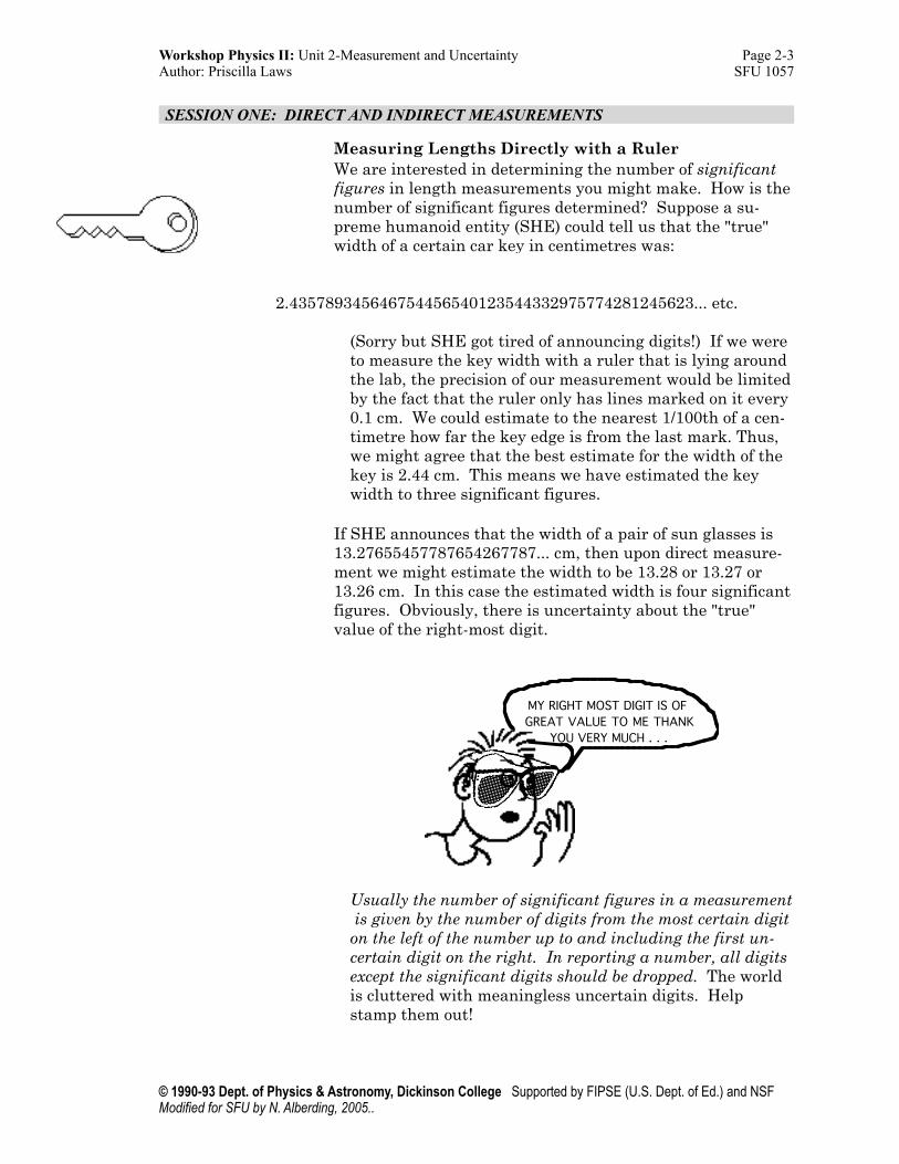
Measuring Lengths Directly with a RulerWe are interested in determining the number of significant figures in length measurements you might make. How is the number of significant figures determined? Suppose a su-preme humanoid entity (SHE) could tell us that the "true" width of a certain car key in centimetres was:

2.435789345646754456540123544332975774281245623... etc.

(Sorry but SHE got tired of announcing digits!) If we were to measure the key width with a ruler that is lying around the lab, the precision of our measurement would be limited by the fact that the ruler only has lines marked on it every 0.1 cm. We could estimate to the nearest 1/100th of a cen-timetre how far the key edge is from the last mark. Thus, we might agree that the best estimate for the width of the key is 2.44 cm. This means we have estimated the key width to three significant figures.

If SHE announces that the width of a pair of sun glasses is 13.27655457787654267787... cm, then upon direct measure-ment we might estimate the width to be 13.28 or 13.27 or 13.26 cm. In this case the estimated width is four significant figures. Obviously, there is uncertainty about the "true" value of the right-most digit.

MY RIGHT MOST DIGIT IS OFGREAT VALUE TO ME THANK

YOU VERY MUCH . . .

Usually the number of significant figures in a measurement is given by the number of digits from the most certain digit on the left of the number up to and including the first un-certain digit on the right. In reporting a number, all digits except the significant digits should be dropped. The world is cluttered with meaningless uncertain digits. Help stamp them out!

Workshop Physics II: Unit 2-Measurement and Uncertainty ! Page 2-3Author: Priscilla Laws SFU 1057

© 1990-93 Dept. of Physics & Astronomy, Dickinson College Supported by FIPSE (U.S. Dept. of Ed.) and NSFModified for SFU by N. Alberding, 2005..

Note: If you have not encountered the idea of significant digits before, you can look up references to this concept in a physics text.

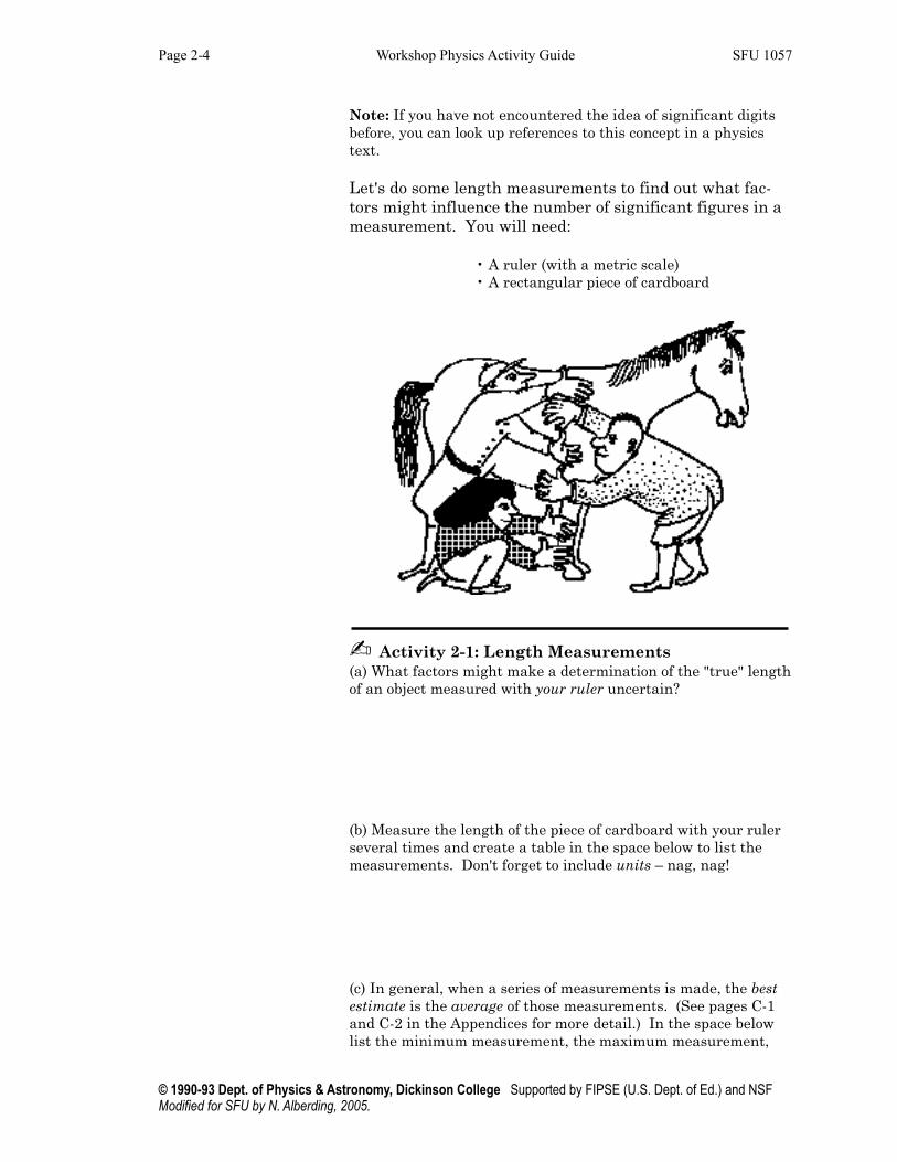
Let's do some length measurements to find out what fac-tors might influence the number of significant figures in a measurement. You will need:

! ! • A ruler (with a metric scale)! ! • A rectangular piece of cardboard

Instructor: Cut the cardboard ends so they are slightly non-parallel.

✍ Activity 2-1: Length Measurements(a) What factors might make a determination of the "true" length of an object measured with your ruler uncertain?

(b) Measure the length of the piece of cardboard with your ruler several times and create a table in the space below to list the measurements. Don't forget to include units – nag, nag!

(c) In general, when a series of measurements is made, the best estimate is the average of those measurements. (See pages C-1 and C-2 in the Appendices for more detail.) In the space below list the minimum measurement, the maximum measurement,

Page 2-4! Workshop Physics Activity Guide! SFU 1057


and the best estimate for the length of your cardboard. Include your units!

l (min) =

l (max) =

l (best est.) =

(d) How many significant figures should you report in your best estimate? Why?

(e) For your piece of cardboard, what limits the number of sig-nificant figures most – variation in the actual length of the card-board or limitations in the accuracy of the ruler? How do you know?

It's clearly impossible to make even the simplest direct dis-tance measurements without some uncertainty. To be able to do so, you would have to have a ruler with an infinite number of lines ruled on it with each line being an impos-sibly short distance from its neighbours!

10 min

Announcing an Indirect Distance Measuring ContestDirect distance measurements are about as straight-forward as measurements can get. Often, however, it's not possible to make a direct measurement, and some ingenuity is needed. Suppose you need to know the height of an object such as a flag pole tip or an interesting feature on a building. How can do it?

You will be assigned a vertical distance to measure on cam-pus with your partners. Prizes will be awarded for the "best" measurements as specified in the Contest Rules listed on the next page.



Contest Rules 1. Students must work in groups, usually three students per group.

2. Each group of students must complete, write up, and submit results jointly for the contest measurement.

3. Only the following equipment can be used for the measurements-

� � • pencil, paper, scotch tape� � • a 15 m long tape rule� � • a digital timer with 1/100th second accuracy� � • a baseball and mitt� � • metre sticks� � • a protractor

4. Measurement write-ups must be received by the deadline date and time announced by the instructor. Each write-up should be placed on an 8.5" by 11" sheet of paper and include:

• the name of all co-operating partners• a description of what distance was being measured with a sketch of the

object being measured etc.• a clear description of the technique used with any necessary equations

and diagrams• a summary of data and calculations• the best estimate of the measurement (usually the average of all the

really "good" measurements)• a discussion of the major sources of uncertainty in the measurement

procedures.

5. Prizes will be awarded in each of the following categories:

a. The smallest relative uncertainty or % discrepancy as determined by comparing your indirectly measured result with an accepted result de-termined by the course instructor(s). The following equation will be used in making the comparison:

€

% discrepancy = | accepted dist. – meas. dist. |accepted dist.

× 100

where the || symbol represents absolute value.

b. The most original method for a measurement that is within at least 10% of the accepted value.

6. No individual can be awarded more than one prize.

10 min Statistics – The Inevitability of UncertaintyIn common terminology there are three kinds of "errors": (1) mistakes or human errors, (2) systematic errors due to



measurement or equipment problems and (3) inherent un-certainties.

✍ Activity 2-3: Error Types(a) Give an example of how a person could make a "mistake" or "human error" while taking a length measurement.

(b) Give an example of how a systematic error could occur be-cause of the condition of the ruler when a set of length measure-ments are being made.

(c) What might cause inherent uncertainties in a length meas-urement?

With care and attention, it is commonly believed that both mistakes and systematic errors can be eliminated com-pletely. However, inherent uncertainties do not result from mistakes or errors. Instead, they can be attributed in part to the impossibility of building measuring equipment that is precise to an infinite number of significant figures. The ruler provides us with an example of this. It can be made better and better, but it always has an ultimate limit of precision.

Another cause of inherent uncertainties is the large num-ber of random variations affecting any phenomenon being studied. For instance, if you repeatedly drop a baseball from the level of the lab table and measure the time of each fall, the measurements will most probably not all be the same. Even if the stop watch was gated electronically so as to be as precise as possible, there would be small fluc-tuations in the flow of currents through the circuits as a result of random thermal motion of atoms and molecules that make up the wires and circuit elements. This could change the stop watch reading from measurement to measurement. The sweaty palm of the experimenter could cause the ball to stick to the hand for an extra fraction of a second, slight air currents in the room could change the



ball's time of fall, vibrations could cause the floor to oscil-late up and down an imperceptible distance, and so on.

20 minRepeated Time-of-Fall DataYou and your partners can take repeated data on the time of fall of a baseball and eventually share it with the rest of the class. In this way, the class can amass a lot of data and study how it varies from some average value for the time-of-fall. For this activity you will need:

! ! • A ball! ! • A stop watch! ! • A 2-metre stick

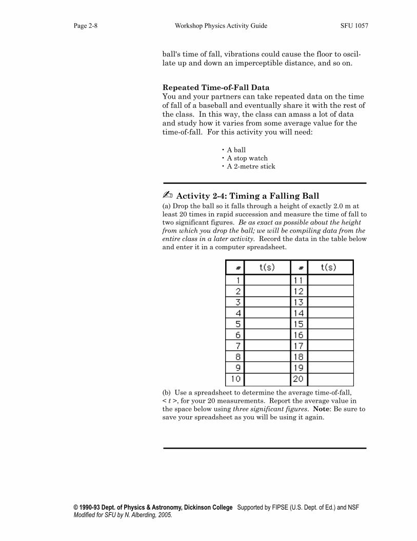
✍ Activity 2-4: Timing a Falling Ball (a) Drop the ball so it falls through a height of exactly 2.0 m at least 20 times in rapid succession and measure the time of fall to two significant figures. Be as exact as possible about the height from which you drop the ball; we will be compiling data from the entire class in a later activity. Record the data in the table below and enter it in a computer spreadsheet.

! ! (b) Use a spreadsheet to determine the average time-of-fall, < t >, for your 20 measurements. Report the average value in the space below using three significant figures. Note: Be sure to save your spreadsheet as you will be using it again.

25 min



The Standard Deviation as a Measure of Uncer-tainty How certain are we that the average fall-time determined in the previous activity is accurate? The average of a number of measurements does not tell the whole story. If all the times you measured were the same, the average would seem to be very precise. If each of the measure-ments varied from the others by a large amount, we would be less certain of the meaning of the average time. We need criteria for determining the certainty of our data. Statisticians often use a quantity called the standard de-viation as a measure of the level of uncertainty in data. In fact, almost all scientific and statistical calculators and spreadsheets have a standard deviation function. The standard deviation is usually represented by the Greek let-ter σ (sigma; since sigma sometimes has other meanings in physics, we will designate the standard deviation by using a subscript: σsd). σsd has a formal mathematical definition which is described in Appendix C. The value of σsd is often used to measure the level of uncertainty in data.

In the next activity you will use the spreadsheet to calcu-late the value of the standard deviation for the repeated fall-time data you just obtained and explore how the stan-dard deviation is related to variation in your data. In par-ticular, you will try to answer this question: What percent-age of your data lies within one standard deviation of the average you calculated?

✍ Activity 2-5: Standard Deviation(a) Open the spreadsheet containing the time-of-fall data you collected in Activity 2-4. Calculate the standard deviation of the set of 20 measurements. (See Appendix C for instructions on how to use spreadsheet functions to calculate quantities such as σsd using a spreadsheet.) Write the calculated value σsd with units in the space below using three significant figures.

� � σsd =

(b) Refer to the average you reported in Activity 2-4(b) and calcu-late the average plus the standard deviation and the average minus the standard deviation. Again report three significant figures and units.

< t > + σsd = ! ! ! < t > – σsd =



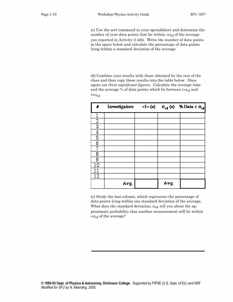
(c) Use the sort command in your spreadsheet and determine the number of your data points that lie within ±σsd of the average you reported in Activity 2-4(b). Write the number of data points in the space below and calculate the percentage of data points lying within a standard deviation of the average.

(d) Combine your results with those obtained by the rest of the class and then copy these results into the table below. Once again use three significant figures. Calculate the average time and the average % of data points which lie between t-σsd and t+σsd.

(e) Study the last column, which represents the percentage of data points lying within one standard deviation of the average. What does the standard deviation, σsd, tell you about the ap-proximate probability that another measurement will lie within ±σsd of the average?

Instructor: Conduct a class discussion. By pooling data, the class should find that there is about a 68% chance of a given data point lying within ± s of the average. THIS GIVES US AN IMPORTANT INTERPRETATION OF THE SIGNIFICANCE OF THIS STRANGE SIGMA OR STANDARD DEVIATION FACTOR. Ask who is the most accurate. The most precise. Why?



SESSION TWO: RANDOM AND SYSTEMATIC VARIATION30 min Go over problems and grading criteria carefully

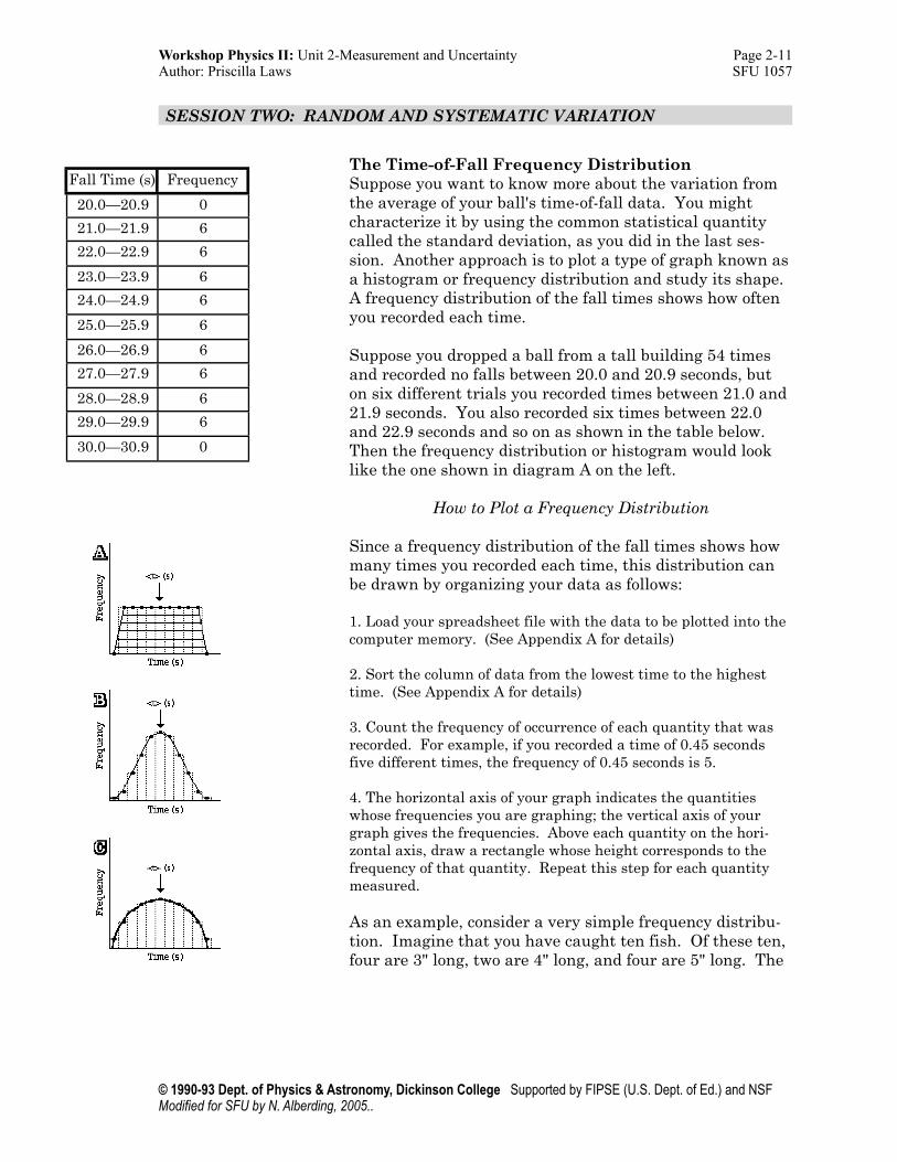
35 minThe Time-of-Fall Frequency DistributionSuppose you want to know more about the variation from the average of your ball's time-of-fall data. You might characterize it by using the common statistical quantity called the standard deviation, as you did in the last ses-sion. Another approach is to plot a type of graph known as a histogram or frequency distribution and study its shape. A frequency distribution of the fall times shows how often you recorded each time.

Suppose you dropped a ball from a tall building 54 times and recorded no falls between 20.0 and 20.9 seconds, but on six different trials you recorded times between 21.0 and 21.9 seconds. You also recorded six times between 22.0 and 22.9 seconds and so on as shown in the table below. Then the frequency distribution or histogram would look like the one shown in diagram A on the left.

How to Plot a Frequency Distribution

Since a frequency distribution of the fall times shows how many times you recorded each time, this distribution can be drawn by organizing your data as follows:

1. Load your spreadsheet file with the data to be plotted into the computer memory. (See Appendix A for details)

2. Sort the column of data from the lowest time to the highest time. (See Appendix A for details)

3. Count the frequency of occurrence of each quantity that was recorded. For example, if you recorded a time of 0.45 seconds five different times, the frequency of 0.45 seconds is 5.

4. The horizontal axis of your graph indicates the quantities whose frequencies you are graphing; the vertical axis of your graph gives the frequencies. Above each quantity on the hori-zontal axis, draw a rectangle whose height corresponds to the frequency of that quantity. Repeat this step for each quantity measured.

As an example, consider a very simple frequency distribu-tion. Imagine that you have caught ten fish. Of these ten, four are 3" long, two are 4" long, and four are 5" long. The



Fall Time (s) Frequency

20.0—20.9 0

21.0—21.9 6

22.0—22.9 6

23.0—23.9 6

24.0—24.9 6

25.0—25.9 6

26.0—26.9 6

27.0—27.9 6

28.0—28.9 6

29.0—29.9 6

30.0—30.9 0

frequency distribution would appear as follows:

4. The horizontal axis of your graph indicates the quantities

whose frequencies you are graphing; the vertical axis of your

graph gives the frequencies. Above each quantity on the

horizontal axis, draw a rectangle whose height corresponds

to the frequency of that quantity. Repeat this step for each

quantity measured.

As an example, consider a very simple frequency

distribution. Imagine that you have caught ten fish.

Of these ten, four are 3" long, two are 4" long, and four

are 5" long. The frequency distribution would appear

as follows:

! Activity 2-7: Frequency Distribution for Your

Time-of-fall Data (a) Draw a frequency diagram (known as a histogram)

representing your time-of-fall data for the ball in the grid

below.

(b) Next, using a different colour

of pen or pencil sketch in the

results of the rest of the class in

the histogram above.

How does the shape of the class

frequency distribution above

compare with the shape shown

in Appendix C on page C-6? !

Does the variation in the time of

fall data seem "normally

distributed"? How does it

compare to your prediction in

Activity 2-6? !Explain.


© 1990-93 Dept. of Physics & Astronomy, Dickinson College Supported by FIPSE (U.S. Dept. of Ed.) and NSF. Modified for SFU by N. Alberding, 2005.

✍ Activity 2-7: Frequency Distribution for Your Time-of-fall Data (a) Draw a frequency diagram (known as a histogram) represent-

ing your time-of-fall data for the ball on the grid.

(b) Next, using a different colour of pen or pencil sketch in the results of the rest of the class in the histogram above.How does the shape of the class frequency distribu-tion above compare with the shape shown in Ap-pendix C on page C-6? Does the variation in the time of fall data seem "normally distributed"? How does it compare to your prediction in Activity 2-6? Explain.

Note: As you will observe later, a normal distribution of varia-tion in a series of measurements can lead to a bell-shaped curve when the variations in measurement are the result of a number of smaller variations which occur randomly from measurement to measurement. Although the underlying events are random, and hence unpredictable, the nature of the variation becomes predictable. Puzzled? Stay tuned, we'll tackle this idea again.

45 min



Systematic Error – How About the Accuracy of Your Timing Device and Timing Methods?As the result of problems with your measuring instrument or the procedures you are using, each of your measure-ments may tend to be consistently too high or too low. If this is the case, you probably have a source of systematic error. There are several types of systematic error.

Most of us have set a watch or clock only to see it gain or lose a certain amount of time each day or week. In ordi-nary language we would say that such a time keeping de-vice is inaccurate. In scientific terms, we would say that it is subject to systematic error. In the case of a stopwatch or digital timer that doesn't run continuously like a clock, we have to ask an additional set of questions. Does it start up immediately? Does it stop exactly when the event is over? Is there some delay in the start and stop time? A delay in starting or stopping a timer could also cause systematic error.

Finally, systematic error can be present as a result of the methods you and your partner are using for making the measurement. For example, are you starting the timer ex-actly at the beginning of the event being measured and stopping it exactly at the end? Are you dropping the ball from a little above the exact starting point each time? A little below?

It is possible to correct for systematic error if you can quantify it. Suppose that God, who is a theoretical physi-cist, said that the distance in metres, y, that a ball falls after a time of t seconds near the earth's surface in most places is given by the equation

! !

€

y =12

gt2

where g is the gravitational strength (equal to 9.8 N/kg). (In this idealized equation the effects of air resistance have been neglected.)

Does the theoretical value for the time-of-fall lie within the standard error of your average measured value? In the activity that follows, you should compare your average time-of-fall with that expected by theory. If you determine that a systematic error probably exists, can you devise a way to determine its cause and magnitude?



✍ Activity 2-8: Is There Systematic Error in the Data?(a) Measure the distance of fall and calculate the theoretical, God given, time-of-fall in the space below.

(b) Does the theoretical value lie in the range of your own aver-age value with its associated uncertainty? If not, you probably have a source of systematic error.

(c) If you seem to have systematic error, explain whether the measured times tend to be too short or too long and list some of the possible causes of it in the space below.

(d) Devise a method to find the causes of your systematic error. Explain what you did in the space below.



SESSION THREE: NORMAL DISTRIBUTIONS AND NUCLEAR DECAY20 min Go over problems that are due.15 min

The Random or Drunkard’s Walk in One DimensionLet's return to the question of how the accumulation of many small random events can lead to a pattern of varia-tions in a series of measurements which is "normally dis-tributed" and thus has a histogram which looks like a bell-shaped curve. To do this we are going to consider a series of measurements on the locations of drunkards in an alley. If the drunkards leave a bar in the centre of the alley and then make many small steps at random where will we find them sleeping in the morning? Assume that during each second of time that passes a drunk has an equal probabil-ity of staggering to the right, standing still, or staggering to the left.

✍ Activity 2-9: The Random Walk — Predictions(a) If a drunk leaves the bar and staggers around taking 30-cm long steps to the right and to the left at random, what will the drunk's average distance in metres from the bar be after he has had a chance to take many steps?

(b) Is it more likely that a drunk will be close to the bar or far away? Why?

(c) Suppose a drunk has had enough time to take 20 steps. Is it possible to find her 20 steps from the bar in either direction? Is it probable? Explain!

Let's simulate the drunkard’s walk scenario and take some data. In this exercise you are to come out of the bar and try to take twenty steps at random. Where are you after at-tempting twenty steps? Each possible step that the drunkard might take is analogous to a source of variation in a measurement in the physics laboratory. For example,



in dropping a ball there might be twenty variables that would effect its rate of fall, e.g., air currents, inconsistent timing, the hand quivering upon release, etc. etc. For the observations that follow you will need:

! • 1 die (six-sided)! • OPTIONAL: a case of beer and an alley

✍ Activity 2-10: The Random Walk – Simulated Ob-servations

(a) Imagine that you have just come out of a bar at the centre of a narrow alley. Roll your die. For 1 or 2 stagger one step to the left. For 3 or 4 just twirl around in the same place. For 5 or 6 take a step to the right. Now where are you? Starting from the new lo-cation roll the die again to take another step. Do this a total of 20 times. Where are you after twenty tries? Eight to the left? Three to the right? etc. Repeat the procedure twice more.

Step ## on

Die

Step (–1,0, or +1)

New

Pos.

1

2

3

4

5

6

7

8

9

10

11

12

13

14

15

16

17

18

19

20

Step ## on

Die

Step (–1,0, or +1)

New

Pos.

1

2

3

4

5

6

7

8

9

10

11

12

13

14

15

16

17

18

19

20

Step ## on

Die

Step (–1,0, or +1)

New

Pos.

1

2

3

4

5

6

7

8

9

10

11

12

13

14

15

16

17

18

19

20

(b) For each "walk" you took in part (a), mark your final position on the histogram below. Also mark the final locations of other drunks in your class. See note below for how to use a spread-sheet to simulate your walk more efficiently.



(c) Does the variation in the data look as if it will be "normally distributed" when each value has an uncertainty that results from the accumulation of many random unpredictable steps?

Simulating the Drunkard’s Walk with a Spreadsheet

Using a spreadsheet to help you take your imaginary walks from the bar is much faster than rolling a die. Most spreadsheets have a built in random function that generates a random number which is greater than or equal to zero and less than 1. By manipulating this function and finding the integer value of the resulting numbers, it is easy to generate an integer with values of -1, 0, and +1. The equations that work for a typical spreadsheet are shown below.

!



By entering these equations into a spreadsheet and recalculating you can simulate multiple 20 second walks. Each simulated walk should take a mere fraction of a second.

5 minNatural Radioactivity and StatisticsWhat happens when the particles coming from radioactive materials are counted during a time interval such as a sec-ond? What variation might we expect in repeated meas-urements? In particular, does the shape of the frequency dis-tribution of the number of counts per second look like that of the repeated measurements of time for a falling ball?

Before exploring these questions, let's briefly review radio-activity. Radioactivity is understood as a phenomenon in which neutrons and protons in a nucleus lose potential en-ergy. Every once in a while, a nucleus in a collection of ra-dioactive atoms ejects either a gamma ray, a beta particle, or an alpha particle. Radioactivity is a statistical process in which a series of slight disturbances of the nucleus lead to a decay.

Heavy elements such as uranium and thorium occur natu-rally in rocks and soil. Even a few tiny grains of such an element can contain hundreds of billions of nuclei that are radioactive. The tiny particles ejected from a sample of radioactive matter can be counted by an electronic device known as a Geiger tube.

5 minPurpose of the Nuclear Counting ExperimentIf a given radioactive nucleus lives on the average for bil-lions of years before undergoing decay, then a collection of many such nuclei will appear, on the average, to give off the same number of particles each second. What will hap-pen if you count the radiation coming into a Geiger tube for one second and then repeat the measurement 20 times, 100 times, ..., 1000 times? Do you expect to see variations?

In this experiment you will count the number of beta parti-cles coming into a Geiger counter during a fixed time in-terval. Then you'll do it again and again and again and again, etc. You can use your measurements to find the av-erage value of your counts per time interval, calculate the standard deviation, and produce a graph of the frequency distribution. The main point of the experiment and its analysis is to compare the shape of the frequency distribu-tion curve for beta particles per time interval to that for fal-ling balls. Are they similar? What happens when you take thousands of "data points?" What does the shape of the fre-quency distribution look like then?



For this experiment you will need a radioactive source, a Geiger tube, and a computer-based laboratory system. The computer system can keep track of particles coming into a Geiger tube automatically. This allows you to take large quantities of data painlessly and thus continue your explo-ration of the characteristics of repeated measurements on quantities subject to random fluctuations.

65 minBecoming Familiar with the Apparatus to Measure Counts per Interval.In the exploration of the statistics of radioactivity, you can use a Computer-Based Laboratory (CBL) set up as a radia-tion counting system. You will need the following equip-ment:

! • Radiation Monitor ! • a computer interface! • a computer! • radiation monitoring software (Logger Pro)! • a small radium, uranium, or thorium source

Note: If you don't have computer radiation monitoring equip-ment the repeated counts can be taken with an old fashioned Geiger Tube and scalar system.

1. Refer to the instructions in Appendix B for details on how to use the computer-based radiation counting system with your computer.

2. Set up the system and play around with the features of the Event Counter software.

3. See what happens when you move the source farther away from the Geiger tube in the RM-4 monitor.

4. Figure out how to change the counting interval and to display counts/interval vs. time in a graph and in a table on the com-puter screen.

Doing the ExperimentFirst you will be determining the counts/interval for twenty intervals and analysing the data statistically in the same way you analysed the time-of-fall data for the ball. Next you will let the computer plot the frequency distribu-tion histogram for you automatically as it collects the data. This will allow you to obtain a frequency distribution for several thousand repeated counts/interval measurements. This in turn will enable you to tell whether or not the bell shaped curve is a reasonable shape for the frequency dis-tribution.



Set up the monitoring system and adjust the distance be-tween the radioactive source and the Geiger Tube and/or the time interval for the counts until the average number of counts/interval is about 20. You can select this time in-terval to be 1/20th of a second, 1/10th of a second, 1/2 of a second, a second, etc. Once the distance from source to de-tector is adjusted to give about 20 counts in the chosen time interval, the source and the Geiger tube should not be bumped or disturbed.

✍ Activity 2-11: Is There Random Variation in the Nuclear Counting Data? (Class Experiment)(a) Count the radiation coming through the Geiger tube for the pre-set time interval you have chosen. Now, repeat the meas-urement 20 times or more using the same time interval. Record how many times you got zero counts per interval, 1 count per interval and so on. Then plot the frequency distribution of your

results on the grid. (b) Determine the aver-age counts/interval and standard deviation from the computer screen or if necessary use a spreadsheet or scientific calculator to determine the standard deviation. (There are many ways to skin a cat!) List the values in the space below.

(c) Determine the per-centage of your data points that lie within ±σsd of the average. Show your calculations below.



We will perform the nuclear counting experiment together as a class experiment so that it will not be necessary to dis-tribute radioactive sources to all the groups.

Figure 2-1: A Radiation Monitoring System

(d) How does this percentage compare with that you found for the falling ball data? What is the "practical meaning" of the standard deviation, σsd, for the nuclear radiation data?

(e) Finally, we take advantage of the power of the computerized radiation monitoring system and set the computer to monitor several thousand repeated counting intervals with an average count of about 20. (Please appreciate the fact that this would take you hours and hours to do manually!) The frequency distri-bution for this large number of data points can be displayed on the computer screen automatically. After you get a graph of the frequency distribution, upload a copy to WebCT assignments. (You can sketch a copy in the space below.)

(f) Study and comment on the shape of the resulting histogram. Does it look like a bell shaped curve? Does nuclear counting seem to have a random variation? Explain

Students should notice that when a large amount of data is taken the average and the standard devia-tion hardly changes but that the frequency distribution looks much "smoother."



Confidence Intervals and Reporting Uncertainty

Standard Deviation of the Mean To get a good estimate of some quantity you need several measurements, and you really want to know how uncertain the average of those several measurements is, since it is the average that you will write down (as a best estimate). This uncertainty in the average is known as the standard deviation of the mean or S.D.M. for short.

It is this quantity that answers the question, "If I repeat the entire series of N measurements and get a second aver-age, when do I have a 68% confidence that this second av-erage to come close to the first one?" The answer is that you should expect a second average (that results from redo-ing the set of measurements) to have a 68% probability of lying within one S.D.M. of the first average you deter-mined. Thus, the S.D.M. is sometimes referred to as a 68% confidence interval.

Once you know the Standard Deviation (S.D.) it is simple to calculate an estimate for the standard deviation of the mean or S.D.M. This is simply the standard deviation of the sample of N measurements divided by the square root of N.

€

S.D.M . =S.D.

N=

σ

N

It is also referred to at times as the standard error. Since the S.D.M. is actually a measure of uncertainty rather than of an error (in the sense of a mistake), we prefer not to use this term.

The 95% Confidence Interval or S(95)Suppose we wanted to be 95% sure rather than 68% sure that another average was in a certain range of an average. In fact, often when you are asked to report data based on measurements, we would like to have you report the mean or average along with a 95% confidence interval with a "±" (plus or minus) sign in front of it. We will use the notation S(95) for this quantity.

If you were to take a several hundred or more of data points, S(95) would be very close to twice the standard de-viation of the mean. For a limited number of measure-



ments, S(95) and twice the S.D.M. are not the same, but they tend to be similar to each other.

✍ Activity 2-12: Calculating the S.D.M. and S(95)(a) In Activity 2-11 (b) we recorded, with the help of the com-puter,

N = _______

measurements of the counts/interval from a long-lived source.

(b) State the average number of counts/interval below.

(c) The computer determined the Standard Deviation, σ, to be

(d) Use the standard deviation obtained for a large number of counting intervals in Activity 2-11 (b) to calculate the Standard Deviation of the Mean ( i.e., the S.D.M.)

(b) Since the number of measurements (i.e., determinations of counts/interval in Activity 2-11 is large, calculate the approxi-mate value of the 95% confidence interval ( i.e., S(95)) for this measurement.

(c) I am confident on the 68% level that if I repeated Activity 2-11 that I would obtain an average that is within

! ! ! _______ ± __________

of the average we obtained.

(d) I am confident on the 95% level that if I repeated Activity 2-11 that I would obtain an average that is within

! ! ! _______ ± __________

of the average we obtained.



UNIT 2 HOMEWORK AFTER SESSION ONE

Before Wednesday September 14 th:

• Start on the Contest Measurement. This year's challenge is shown in the box below. The write-ups are due at the beginning of Session Three on Friday September 16th.• Read Chapter 1 of the textbook with special attention to sections 1-9 and 1-10.

• Read Appendix C of the Activity Guide

• Work Chapter 1 Problems 8, 12, 20, and 26. Be sure to report the correct number of signifi-cant figures.

• Do Problem SP2-1 below, in which you must calculate a standard deviation by hand using the theoretical formula. This is the last time you'll have to do it the hard way in this course. Just in case you get stuck on a desert island with no computer, you'll know how to do it!

SP2-1) Suppose you made the following five length measurements (N=5) of the width of a piece of letter size paper which has been cut carefully by a manufacturer using an unfamiliar centimetre rule: 21.3 cm, 21.5 cm, 21.4. cm, 21.2 cm, 21.4 cm. (a) Use the procedures on pages C-5 through the top of page C-9 of Appendix C find the average and standard deviation of the measurements to four significant figures. Be-ware: N is neither 12 nor 8. (b) Is there any evidence of uncertainty in the measurements or are they pre-cise? Explain. (c) Is there any evidence of systematic error in the measurements? If so, what might cause this? Explain



The Three Guardian Lamps

The plaza in front of the Surrey Central Mall is guarded by three gigantic lamp fixtures. Your job is to measure the vertical distance from the top of the concrete base to the highest point on the reflectors. Remember that direct measurements are forbidden. No fair climbing to the top (even if you could). We assume all three are the same height, but we will use the middle one as reference for the “accepted value”.

Top of concrete

base

UNIT 2 HOMEWORK AFTER SESSION TWO

Before Friday September 16th:

• Complete the Contest Measurements. Write them up according to the specifications in the con-test rules. This write up is worth up to 40 problem credits to each partner (i.e., it is equivalent to solving 4 problems).

• Do Problem SP2-3 below

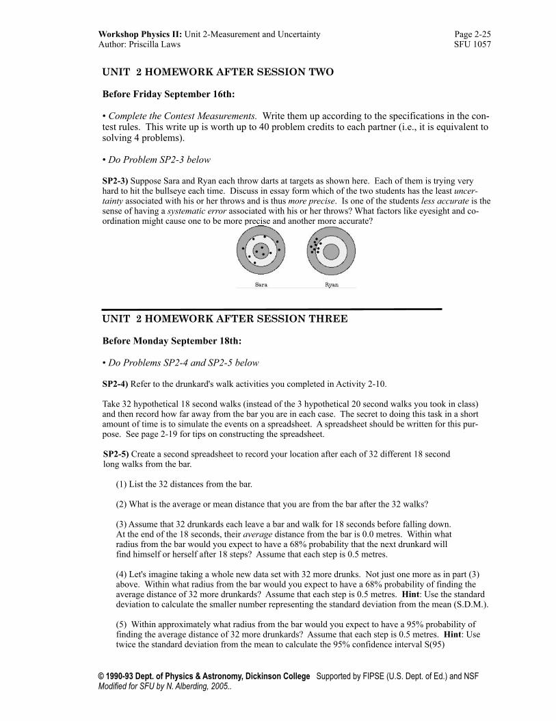
SP2-3) Suppose Sara and Ryan each throw darts at targets as shown here. Each of them is trying very hard to hit the bullseye each time. Discuss in essay form which of the two students has the least uncer-tainty associated with his or her throws and is thus more precise. Is one of the students less accurate is the sense of having a systematic error associated with his or her throws? What factors like eyesight and co-ordination might cause one to be more precise and another more accurate?

UNIT 2 HOMEWORK AFTER SESSION THREE

Before Monday September 18th:

• Do Problems SP2-4 and SP2-5 below

SP2-4) Refer to the drunkard's walk activities you completed in Activity 2-10.

Take 32 hypothetical 18 second walks (instead of the 3 hypothetical 20 second walks you took in class) and then record how far away from the bar you are in each case. The secret to doing this task in a short amount of time is to simulate the events on a spreadsheet. A spreadsheet should be written for this pur-pose. See page 2-19 for tips on constructing the spreadsheet.

SP2-5) Create a second spreadsheet to record your location after each of 32 different 18 second long walks from the bar.

(1) List the 32 distances from the bar.

(2) What is the average or mean distance that you are from the bar after the 32 walks?

(3) Assume that 32 drunkards each leave a bar and walk for 18 seconds before falling down. At the end of the 18 seconds, their average distance from the bar is 0.0 metres. Within what radius from the bar would you expect to have a 68% probability that the next drunkard will find himself or herself after 18 steps? Assume that each step is 0.5 metres.

(4) Let's imagine taking a whole new data set with 32 more drunks. Not just one more as in part (3) above. Within what radius from the bar would you expect to have a 68% probability of finding the average distance of 32 more drunkards? Assume that each step is 0.5 metres. Hint: Use the standard deviation to calculate the smaller number representing the standard deviation from the mean (S.D.M.).

(5) Within approximately what radius from the bar would you expect to have a 95% probability of finding the average distance of 32 more drunkards? Assume that each step is 0.5 metres. Hint: Use twice the standard deviation from the mean to calculate the 95% confidence interval S(95)



UNIT 2: MEASUREMENT AND UNCERTAINTY · the lab, the precision of our ... measurements. Don't forget...

Documents

Transcript of UNIT 2: MEASUREMENT AND UNCERTAINTY · the lab, the precision of our ... measurements. Don't forget...