Stage-Structured Lefkovitch Matrix Population Modeling Learning Objectives: 1. Set up a model of population growth with stage structure. 2. Determine the stable stage distribution of the population. 3. Estimate λ from Lefkovitch matrix calculations. 4. Construct and interpret the stage distribution graphs. 5. Learn more about how to use the remarkable functionality of Excel

2013 to plot and analyze wildlife population data. Introduction The growth rate of the population over discrete time steps is called the geometric growth rate (λ) and describes abundance next year as a proportion of the abundance this year. When λ = 1, a population remains constant in size over time, meaning that it neither increases nor decreases. When λ < 1, a population declines geometrically (i.e., if λ = 0.75 the population will be three-quarters the size than it was last year; that is, the population will decline by 25%). When λ > 1, a population increases geometrically (i.e., if λ = 1.25 the population will be one-quarter larger in size than it was last year; that is, the population will increase by 25%). Mathematically, the abundance of a population (N) at time t+1 is a function of both abundance at time t and the population growth rate: Nt+1 = Nt λ, Equation 1 where N is the number of individuals present in the population, and t is a time interval of interest. This equation says that the size of a population at time t+1 is equal to the size of the population at time t multiplied by a constant, λ. Although geometric growth models have been used to describe population growth, like all models they come with a set of assumptions. What are the assumptions of the geometric growth model? The equation describes a population in which there is no genetic structure, no age structure, and no sex structure (Gotelli 2001), and all individuals are reproductively active when the animals are counted. The model also assumes that resources are virtually unlimited and that growth is unaffected by the size of the population. Can you think of an organism whose life history meets these assumptions? Many

2

natural populations violate at least 1 of these assumptions because wildlife populations are structured—they are composed of individuals whose birth and death rates differ depending on age, size, sex, stage, or genetic make-up. For example, small fish in a population differ in mortality rates from large fish, and larval insects differ in birth rates from adult insects. All else being equal, a population of 1000 individuals that is composed of 350 pre-reproductive-age individuals, 500 reproductive-age individuals, and 150 post-reproductive-age individuals will have a different growth rate than a population where all 1000 individuals are of reproductive age. In this exercise, you will develop a matrix model to explore the growth of populations that have size or stage structure. This approach will enable you to estimate λ in Equation 1 for size- or stage-structured populations. Structured population-projection modeling is discussed in chapter 7 in Mills (2007) and in chapter 6 in Mills (2013). In the “Life Tables, Survivorship Curves, and Population Growth” problem set, you learned that age structure is often a critical variable in determining the size of a population over time. In fact, a primary goal of life table analysis and matrix modeling is to estimate a population’s λ when the population has age structure. For many organisms, however, age is not an accurate predictor of birth or death rates. For example, a small sugar maple in a northeastern forest can be 50 years old and yet have low levels of reproduction. In this species, size is a better predictor of birth rate than age. In other species, birth and death rates are a function of the stage in the life cycle of an organism. For instance, death rates in some insect species may be higher in the larval stages than in the adult stage. Such organisms are best modeled with size- or stage-structured matrix models. Model Notation We begin this exercise with some notation often used when modeling structured populations (Caswell 2001, Gotelli 2001). For modeling purposes, the first decision is whether to develop a stage-structured or a size-structured model for the organism of interest. This in turn depends on whether size or life-history stage is a better state variable. The second step is to assign individuals in the population to either stage or size classes. It is fairly straightforward to categorize individuals with stage structure, such as insects—simply place them in the appropriate stage, such as larva, pupa, or adult. Size, however, is a continuous variable because it is

3

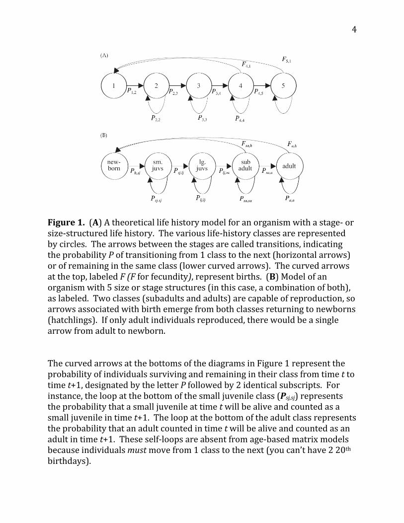
not an either/or situation, but can take on a range of values. In our sugar maple example, size classes might consist of seedlings, small-sized individuals, medium-sized individuals, and large-sized individuals. The number of size classes you select for your model would depend on how different groups “perform” in terms of reproduction and survival. If medium- and large-sized individuals have the same reproductive and survival rates, we might choose to lump them into a single class. Note that the projection interval (the amount of time that elapses between time t and time t+1) and the stage durations can be different. For instance, the larval stage may typically last 4 months, and the pupa stage might typically last only 2 months, and the projection interval may also be different. This is different from age-based matrix models in which the interval of the different classes, as well as the projection interval from time step to time step, must be equal. A typical life cycle model for a species with stage or size structure is shown in Figure 1. The horizontal arrows between each stage (circles) represent survival probabilities, or the probability that an individual in stage/size class i will survive and move into stage/size class i+1, survival probabilities are designated by the letter P followed by 2 different subscripts.

4

Figure 1. (A) A theoretical life history model for an organism with a stage- or size-structured life history. The various life-history classes are represented by circles. The arrows between the stages are called transitions, indicating the probability P of transitioning from 1 class to the next (horizontal arrows) or of remaining in the same class (lower curved arrows). The curved arrows at the top, labeled F (F for fecundity), represent births. (B) Model of an organism with 5 size or stage structures (in this case, a combination of both), as labeled. Two classes (subadults and adults) are capable of reproduction, so arrows associated with birth emerge from both classes returning to newborns (hatchlings). If only adult individuals reproduced, there would be a single arrow from adult to newborn. The curved arrows at the bottoms of the diagrams in Figure 1 represent the probability of individuals surviving and remaining in their class from time t to time t+1, designated by the letter P followed by 2 identical subscripts. For instance, the loop at the bottom of the small juvenile class (Psj,sj) represents the probability that a small juvenile at time t will be alive and counted as a small juvenile in time t+1. The loop at the bottom of the adult class represents the probability that an adult counted in time t will be alive and counted as an adult in time t+1. These self-loops are absent from age-based matrix models because individuals must move from 1 class to the next (you can’t have 2 20th birthdays).

5

The curved arrows at the top of the diagrams represent births, designated by the letter F followed by 2 different subscripts. The arrows all lead to the first class because newborns, by definition, enter the first class upon birth. Note that for both P and F, the subscripts have a definite pattern: the first subscript is the class from which individuals move, and the second subscripts indicate the class to which individuals move (Gotelli 2001). The Lefkovitch Matrix Now let’s discuss the computations of P, F, and λ for a population with stage structure. The major goal of the matrix model is to compute λ, the finite rate of increase, for a population with stage structure (Equation 1). In our matrix model, we can compute the time-specific growth rate, λt, by rearranging terms in Equation 1:

Equation 2

This time-specific growth rate is not necessarily the same λ in Equation 1, but in our spreadsheet model we will compute it in order to arrive at λ (no subscript) in Equation 1. We will discuss this important point later. To determine Nt and Nt+1, we need to count individuals at some standardized time period over time. We’ll assume for this exercise that our population surveys are completed immediately after individuals breed (a postbreeding survey). The number of individuals in the population in a census at time t+1 will depend on how many individuals of each size class were in the population at time t, as well as the movements of individuals into new classes (by birth or transition) or out of the system (by mortality). Thus, in size- or stage-structured models, an individual in any class may move to the next class (i.e., grow larger), remain in their current class, or exit the system (i.e., die). The survival probability, Pi,i+1, is the probability that an individual in size class i will survive and move into size class i+1. In our example, let’s assume that small juveniles survive and become large juveniles with a probability of Psj,lj = 0.3. This means that 30% of the small juveniles in 1 time step will survive to be counted as large juveniles in the next time step. The remaining 70% of the

6

individuals either die or remain small juveniles. Pi,i, is the probability that an individual in size class i will survive to be counted in the next time step, but will remain in size class i. Thus, an individual in size class i may survive and grow to size class i+1 with probability Pi,i+1, or may survive and remain in size class i with probability Pi,i (Caswell 2001). In order to keep track of how many individuals are present in a given class at a given time, we must consider both kinds of survival probabilities to account for those individuals that graduated into the class, plus those individuals that remained in the class (i.e., did not graduate). For example, we can compute the number of individuals in the large juvenile size class at time t+1 as the number of small juveniles at time t multiplied by Psj,lj (this gives the number of small juveniles in year t that graduated to become large juveniles in year t+1), plus the number of large juveniles at time t multiplied by Plj,lj (this gives the number of large juveniles in year t that remained in the large juvenile class in year t+1). More generally speaking, the number of individuals in class i in year t+1 will be

Equation 3 Equation 3 works for calculating the number of individuals at time t+1 for each size class in the population except for the first, because individuals in the first stage class at time t + 1 will include those individuals in class 1 that remain in class 1 in the next time step, plus any new individuals that arise through birth. Accordingly, let’s now consider birth rates. There are many ways to describe the births in a population. Here we will assume a simple birth-pulse model, in which individuals give birth as soon as they enter a new stage class. On this day, not only do births occur, but transitions from one size class to another also occur. When populations are structured, the birth rate is often called the fecundity, or the average number of offspring born per unit time to an individual female of a particular age (Gotelli 2001). In the life table problem set you might recall that fecundity is labeled as b(x), where b is for birth. Individuals that are of pre- or postreproductive age have fecundities of 0. Individuals of reproductive age typically have fecundities greater than 0.

7

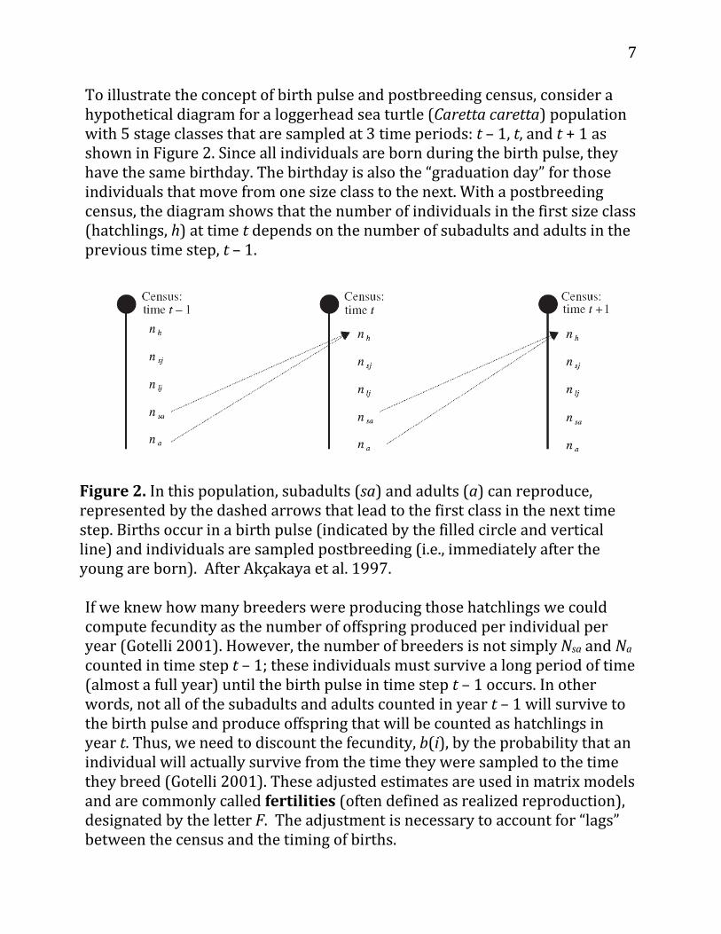
To illustrate the concept of birth pulse and postbreeding census, consider a hypothetical diagram for a loggerhead sea turtle (Caretta caretta) population with 5 stage classes that are sampled at 3 time periods: t – 1, t, and t + 1 as shown in Figure 2. Since all individuals are born during the birth pulse, they have the same birthday. The birthday is also the “graduation day” for those individuals that move from one size class to the next. With a postbreeding census, the diagram shows that the number of individuals in the first size class (hatchlings, h) at time t depends on the number of subadults and adults in the previous time step, t – 1.

Figure 2. In this population, subadults (sa) and adults (a) can reproduce, represented by the dashed arrows that lead to the first class in the next time step. Births occur in a birth pulse (indicated by the filled circle and vertical line) and individuals are sampled postbreeding (i.e., immediately after the young are born). After Akçakaya et al. 1997. If we knew how many breeders were producing those hatchlings we could compute fecundity as the number of offspring produced per individual per year (Gotelli 2001). However, the number of breeders is not simply Nsa and Na counted in time step t – 1; these individuals must survive a long period of time (almost a full year) until the birth pulse in time step t – 1 occurs. In other words, not all of the subadults and adults counted in year t – 1 will survive to the birth pulse and produce offspring that will be counted as hatchlings in year t. Thus, we need to discount the fecundity, b(i), by the probability that an individual will actually survive from the time they were sampled to the time they breed (Gotelli 2001). These adjusted estimates are used in matrix models and are commonly called fertilities (often defined as realized reproduction), designated by the letter F. The adjustment is necessary to account for “lags” between the census and the timing of births.

8

These adjustments are a bit trickier for stage-based than for age-based models because both kinds of survival probabilities (Pi,i+1 and Pi,i) come into play. For example, suppose we want to compute the fertility rate of subadults, Fsa that were sampled in year t. We need to ask, “How many offspring are produced, on average, per subadult sampled in year t?” To answer this question, we need to know how many subadults were counted during the census for year t, how many of those individuals survived to the birth pulse in the same time step, and the total number of young produced by those individuals. Keeping in mind that the graduation day is the same day as the birth pulse, the young produced by the breeding individuals comes from 2 sources: (1) those subadults that survived to the birth pulse and reproduced at the rate of subadults (bi × Pi,i), and (2) those subadults that survived to the birth pulse and graduated to adulthood and reproduced as adults (bi+1 × Pi,i+1). Accordingly, we can compute the fertility rate as

Equation 4

Thus, Fi indicates the number of young that are produced per female of stage i in year t, given the appropriate adjustments (Caswell 2001). The total number of individuals counted in stage 1 (newborns or hatchlings) in year t + 1 is simply the fertility rate of each age class, multiplied by the number of individuals in that size class at time t, plus any individuals that remained in the first size class from one time step to the next. Generally speaking,

Equation 5

Once we know the fertility and survivorship coefficients for each age class, we can calculate the number of individuals in each age at time t + 1, given the number of individuals in each class at time t (Gotelli 2001):

9

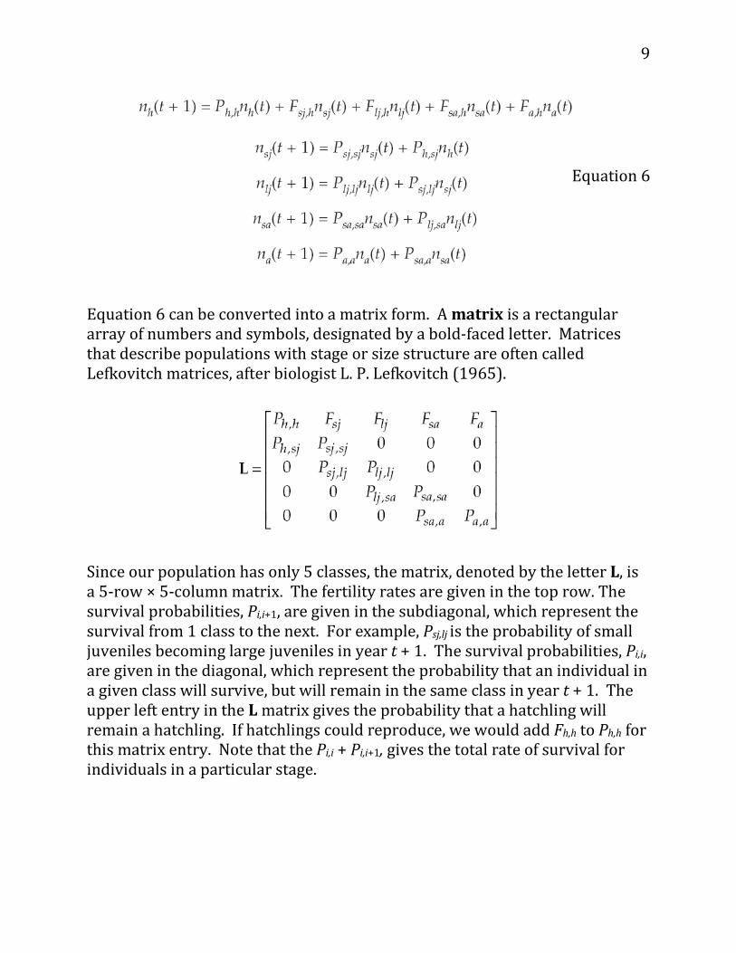
Equation 6 Equation 6 can be converted into a matrix form. A matrix is a rectangular array of numbers and symbols, designated by a bold-faced letter. Matrices that describe populations with stage or size structure are often called Lefkovitch matrices, after biologist L. P. Lefkovitch (1965).

Since our population has only 5 classes, the matrix, denoted by the letter L, is a 5-row × 5-column matrix. The fertility rates are given in the top row. The survival probabilities, Pi,i+1, are given in the subdiagonal, which represent the survival from 1 class to the next. For example, Psj,lj is the probability of small juveniles becoming large juveniles in year t + 1. The survival probabilities, Pi,i, are given in the diagonal, which represent the probability that an individual in a given class will survive, but will remain in the same class in year t + 1. The upper left entry in the L matrix gives the probability that a hatchling will remain a hatchling. If hatchlings could reproduce, we would add Fh,h to Ph,h for this matrix entry. Note that the Pi,i + Pi,i+1, gives the total rate of survival for individuals in a particular stage.

10

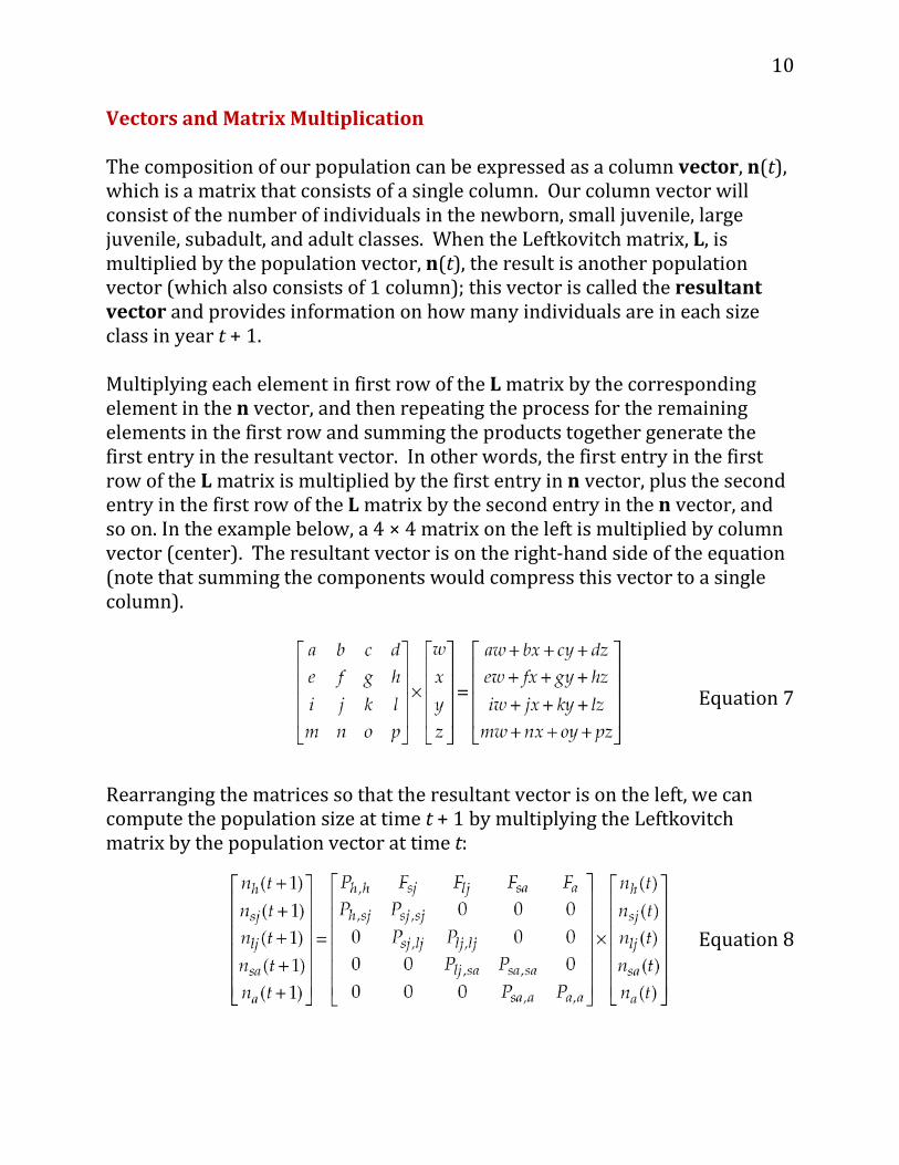
Vectors and Matrix Multiplication The composition of our population can be expressed as a column vector, n(t), which is a matrix that consists of a single column. Our column vector will consist of the number of individuals in the newborn, small juvenile, large juvenile, subadult, and adult classes. When the Leftkovitch matrix, L, is multiplied by the population vector, n(t), the result is another population vector (which also consists of 1 column); this vector is called the resultant vector and provides information on how many individuals are in each size class in year t + 1. Multiplying each element in first row of the L matrix by the corresponding element in the n vector, and then repeating the process for the remaining elements in the first row and summing the products together generate the first entry in the resultant vector. In other words, the first entry in the first row of the L matrix is multiplied by the first entry in n vector, plus the second entry in the first row of the L matrix by the second entry in the n vector, and so on. In the example below, a 4 × 4 matrix on the left is multiplied by column vector (center). The resultant vector is on the right-hand side of the equation (note that summing the components would compress this vector to a single column).

Equation 7 Rearranging the matrices so that the resultant vector is on the left, we can compute the population size at time t + 1 by multiplying the Leftkovitch matrix by the population vector at time t:

Equation 8

11

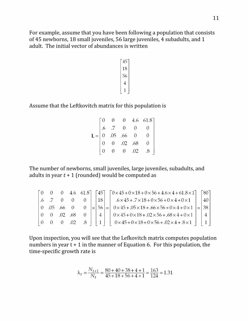
For example, assume that you have been following a population that consists of 45 newborns, 18 small juveniles, 56 large juveniles, 4 subadults, and 1 adult. The initial vector of abundances is written

Assume that the Leftkovitch matrix for this population is

The number of newborns, small juveniles, large juveniles, subadults, and adults in year t + 1 (rounded) would be computed as

Upon inspection, you will see that the Lefkovitch matrix computes population numbers in year t + 1 in the manner of Equation 6. For this population, the time-specific growth rate is

12

The Lefkovitch matrix not only allows you to calculate λ1 but also lets you evaluate how the composition of the population changes from 1 time step to the next. If you continued projecting the population dynamics into the future, you would be able to ascertain how the population “behaves” if the present conditions (P’s and F’s) were to be maintained indefinitely (Caswell 2001). Continued multiplication of a vector of abundance by the Lefkovitch matrix eventually produces a population with a stable size or stable stage distribution, where the proportion of individuals in each stage remains constant over time, and there is a stable (unchanging) finite rate of increase, λ1. When the λ1’s converge to a constant value, this constant is an estimate of λ in Equation 1, and is called the asymptotic growth rate. At this point, if the population is growing or declining, all stage classes grow or decline at the same rate, even if the numbers of individuals in each class are different. You will see how this happens as you work through the exercise. Instructions In this exercise, you will develop a stage-based model for loggerhead sea turtles (Caretta caretta). In this population, the size stages are hatchlings (h), small juveniles (sj), large juveniles (lj), subadults (sa), adults (a). Turtles are counted every year in a post-breeding survey, where the numbers of individuals in each stage class are tallied. A. Set up the model population

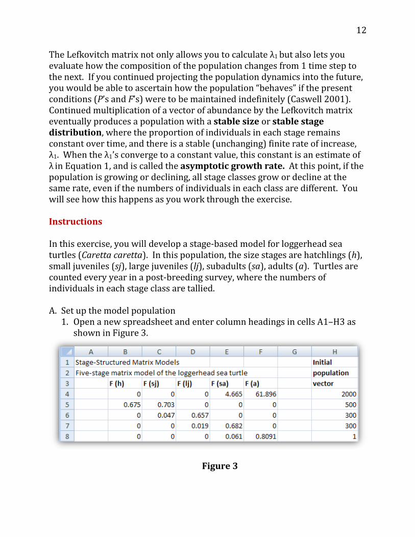
1. Open a new spreadsheet and enter column headings in cells A1–H3 as shown in Figure 3.

Figure 3

13

2. Enter the values shown in Figure 3 for cells B4–F8. Write your interpretation of what each cell value means in the table below. These are the matrix values derived by Crowder et al. (1994). For example, the value in cell B5 is the probability that a hatchling in year t will become a small juvenile in year t + 1.

3. Enter the values for cells H4–H8 as shown in Figure 3. These values

make up the initial population vector, or how many individuals of each stage are currently in the population.

4. Set up new column headings as shown in Figure 4 and set up a linear series in column A that will track abundances of individuals for 100 years. Enter 0 in cell A11. Enter the formula =A11+1 in cell A12. Copy this formula down to cell A111 to simulate 100 years of population growth.

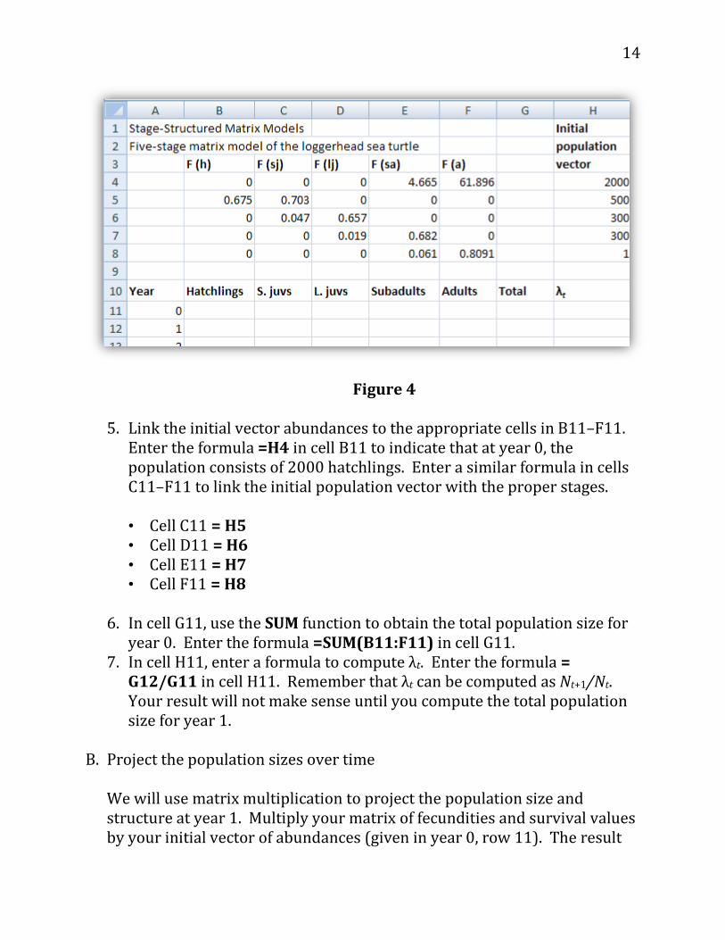
14

Figure 4

5. Link the initial vector abundances to the appropriate cells in B11–F11. Enter the formula =H4 in cell B11 to indicate that at year 0, the population consists of 2000 hatchlings. Enter a similar formula in cells C11–F11 to link the initial population vector with the proper stages.

• Cell C11 = H5 • Cell D11 = H6 • Cell E11 = H7 • Cell F11 = H8

6. In cell G11, use the SUM function to obtain the total population size for

year 0. Enter the formula =SUM(B11:F11) in cell G11. 7. In cell H11, enter a formula to compute λt. Enter the formula =

G12/G11 in cell H11. Remember that λt can be computed as Nt+1/Nt. Your result will not make sense until you compute the total population size for year 1.

B. Project the population sizes over time

We will use matrix multiplication to project the population size and structure at year 1. Multiply your matrix of fecundities and survival values by your initial vector of abundances (given in year 0, row 11). The result

15

will be the number of individuals in the next generation that are hatchlings, small juveniles, large juveniles, subadults, and adults. Recall how matrices are multiplied: The L matrix is located on the left, and is multiplied by the initial vector of abundances (v). The result is a new vector of abundances for the year t + 1. Refer to Equations 7 and 8. (Equation 7 is a 4 × 4 matrix; you will carry out the multiplication for a 5 × 5 matrix.)

1. Enter a formula in cell B12 to obtain the number of hatchlings in year 1.

Enter the formula =$B$4*B11+$C$4*C11+$D$4*D11+$E$4*E11+$F$4*F11 in cell B12. Make sure you refer to the initial abundances listed in row 11 in your formula, rather than the initial abundances listed in column H.

2. Enter formulas in cells C12–F12 to obtain the number of small juveniles, large juveniles, subadults, and adults in year 1. Use the following formulas:

• Cell C12 =$B$5*B11+$C$5*C11+$D$5*D11+$E$5*E11+$F$5*F11 • Cell D12 =$B$6*B11+$C$6*C11+$D$6*D11+$E$6*E11+$F$6*F11 • Cell E12 =$B$7*B11+$C$7*C11+$D$7*D11+$E$7*E11+$F$7*F11 • Cell F12 =$B$8*B11+$C$8*C11+$D$8*D11+$E$8*E11+$F$8*F11

3. In cell G12, use the SUM function to sum the individuals in the different

stages. Enter the formula =SUM(B12:F12) in cell G12. 4. In cell H12, calculate the time-specific growth rate, λt. Copy cell H11

into H12. When λt = 1, the population remained constant in size. When λt < 1, the population declined, and when λt >1, the population increased in numbers.

5. Select cells B12–H12, and copy the formulae down to cells B111–H111. This will complete a 100-year simulation of stage-structured population growth. Click on a few random cells and make sure you can interpret the formulae and how they work.

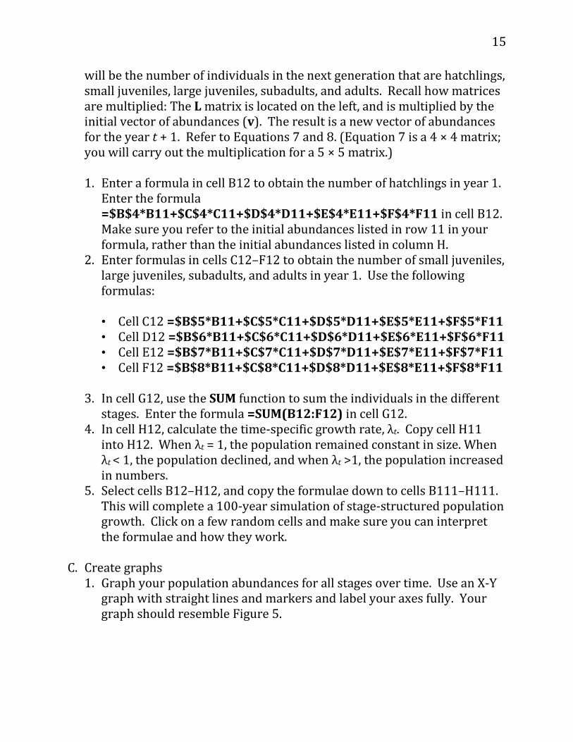
C. Create graphs

1. Graph your population abundances for all stages over time. Use an X-Y graph with straight lines and markers and label your axes fully. Your graph should resemble Figure 5.

16

Figure 5

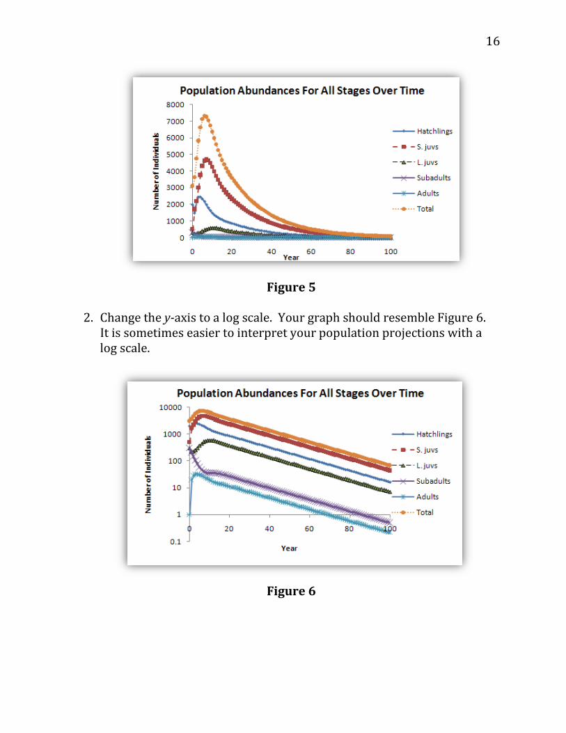
2. Change the y-axis to a log scale. Your graph should resemble Figure 6. It is sometimes easier to interpret your population projections with a log scale.

Figure 6

17

Discussion Questions 1. What are the assumptions of the model you have built? 2. At what point in the 100-year simulation does λt not change (or change

very little) from year to year? This constant is an estimate of the asymptotic growth rate, λ, from Equation 1. What value is λ? Given this value of λ, how would you describe population growth of the sea turtle population?

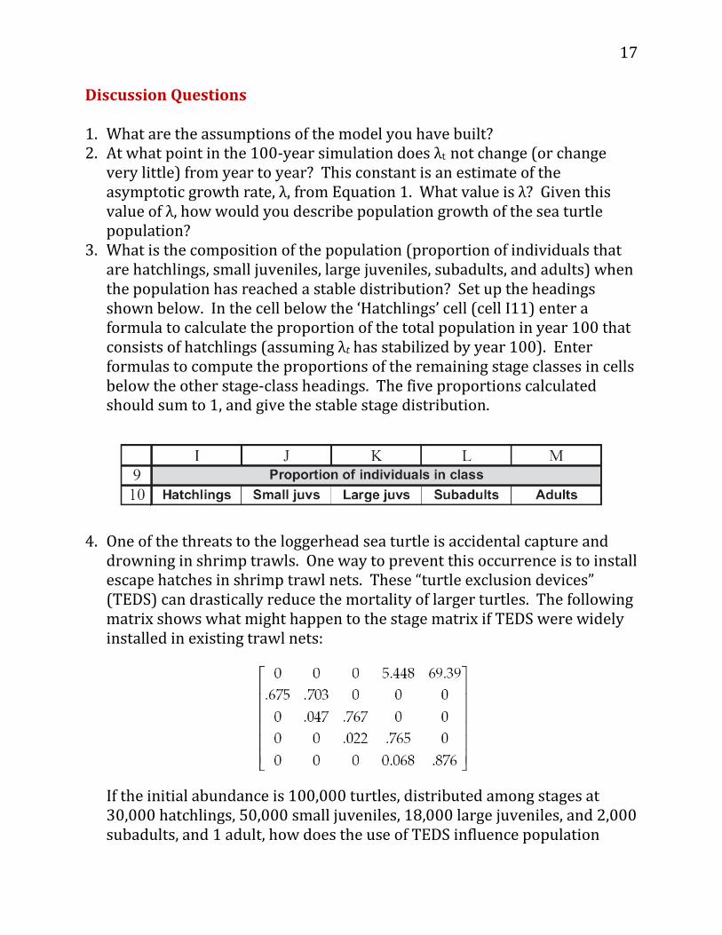
3. What is the composition of the population (proportion of individuals that are hatchlings, small juveniles, large juveniles, subadults, and adults) when the population has reached a stable distribution? Set up the headings shown below. In the cell below the ‘Hatchlings’ cell (cell I11) enter a formula to calculate the proportion of the total population in year 100 that consists of hatchlings (assuming λt has stabilized by year 100). Enter formulas to compute the proportions of the remaining stage classes in cells below the other stage-class headings. The five proportions calculated should sum to 1, and give the stable stage distribution.

4. One of the threats to the loggerhead sea turtle is accidental capture and

drowning in shrimp trawls. One way to prevent this occurrence is to install escape hatches in shrimp trawl nets. These “turtle exclusion devices” (TEDS) can drastically reduce the mortality of larger turtles. The following matrix shows what might happen to the stage matrix if TEDS were widely installed in existing trawl nets:

If the initial abundance is 100,000 turtles, distributed among stages at 30,000 hatchlings, 50,000 small juveniles, 18,000 large juveniles, and 2,000 subadults, and 1 adult, how does the use of TEDS influence population

18

dynamics? Provide a graph and discuss your answer in terms of population size, structure, and growth. Discuss how the use of TEDS affects the F and P parameters in the Lefkovitch matrix.

Literature Cited Akçakaya, H. R., M. A. Burgman, and L. R. Ginzburg. 1997. Applied population

ecology. Applied Biomathematics, Setauket, New York, USA. Caswell, H. 2001. Matrix population models, 2nd Edition. Sinauer Associates,

Sunderland, Massachusetts, USA. Crowder, L. B., D. T. Crouse, S. S. Heppell, and T. H. Martin. 1994. Predicting the

impact of turtle excluder devices on loggerhead turtle populations. Ecological Applications 4: 437–445.

Gotelli, N. 2001. A primer of ecology, 3rd Edition. Sinauer Associates,

Sunderland, Massachusetts, USA. Lefkovitch, L. P. 1965. The study of population growth in organisms grouped

by stages. Biometrika 35: 183–212. Acknowledgement This problem set was adapted from Exercise 14: Stage-structured matrix models, pages 187-199 in Donovan, T. M. and C. Welden. 2002. Spreadsheet exercises in ecology and evolution. Sinauer Associates, Inc. Sunderland, MA, USA. This publication is available at http://www.uvm.edu/rsenr/vtcfwru/spreadsheets/?Page=ecologyevolution/EE24.htm. Your write-up should include the following: (1) a paragraph explaining the objectives of this problem set, and (2) your answers to the 4 discussion questions above. Email me (whited@uamont.edu) your spreadsheet model.