Robust Control - pdfs.semanticscholar.org · Robust Control Ad Damen and Siep Weiland (tekst bij...
206
Robust Control Ad Damen and Siep Weiland (tekst bij het college: Robuuste Regelingen 5P430, najaarstrimester) Measurement and Control Group Department of Electrical Engineering Eindhoven University of Technology P.O.Box 513 5600 MB Eindhoven Draft version of July 17, 2002
Transcript of Robust Control - pdfs.semanticscholar.org · Robust Control Ad Damen and Siep Weiland (tekst bij...

Robust Control
Ad Damen and Siep Weiland
(tekst bij het college:Robuuste Regelingen
5P430, najaarstrimester)
Measurement and Control GroupDepartment of Electrical EngineeringEindhoven University of Technology
P.O.Box 5135600 MB Eindhoven
Draft version of July 17, 2002

2

Preface
Opzet
Dit college heeft het karakter van een werkgroep. Dit betekent dat u geen kant en klareportie ‘wetenschap’ ter bestudering krijgt aangeboden, maar dat van u een actieve partic-ipatie zal worden verwacht in de vorm van bijdragen aan discussies en presentaties. In ditcollege willen we een overzicht aanbieden van moderne, deels nog in ontwikkeling zijnde,technieken voor het ontwerpen van robuuste regelaars voor dynamische systemen.
In de eerste helft van het trimester zal de theorie over robuust regelaarontwerp aande orde komen in reguliere hoorcolleges. Als voorkennis is vereist de basis klassieke regel-techniek en wordt aanbevolen kennis omtrent LQG-control en matrixrekening/functionaalanalyse. In het college zal de nadruk liggen op het toegankelijk maken van robuust rege-laarontwerp voor regeltechnici en niet op een uitputtende analyse van de benodigde math-ematiek. Voor deze periode zijn zes oefenopgaven in het dictaat verwerkt, die bedoeld zijnom u ervaring op te laten doen met zowel theoretische als praktische aspecten m.b.t. ditonderwerp.
De bruikbaarheid en de beperkingen van de theorie zullen vervolgens worden getoetstaan diverse toepassingen die in de tweede helft van het college door u en uw collega-studenten worden gepresenteerd en besproken. De opdrachten zijn deels opgezet voorindividuele oplossing en deels voor uitwerking in koppels. U kunt hierbij een keuze makenuit :
• het kritisch evalueren van een artikel uit de toegepast wetenschappelijke literatuur
• een regelaarontwerp voor een computersimulatie
• een regelaarontwerp voor een laboratoriumproces.
Meer informatie hierover zal op het eerste college worden gegeven alwaar intekenlijstengereed liggen.
Iedere presentatie duurt 45 minuten, inclusief discussietijd. De uren en de verroost-ering van de presentaties zullen nader bekend worden gemaakt. Benodigd materiaal voorde presentaties (sheets, pennen, e.d.) zullen ter beschikking worden gesteld en zijn verkri-jgbaar bij het secretariaat van de vakgroep Meten en Regelen (E-hoog 4.32 ). Er wordtverwacht dat u bij tenminste 13 presentaties aanwezig bent en dat u aktief deelneemt aande discussies. Een presentielijst zal hiervoor worden bijgehouden.
Over uw bevindingen t.a.v. het door u gekozen onderwerp wordt een eindgesprekgehouden, waar uit de discussie moet blijken of U voldoende inzicht en ervaring hebtopgedaan. Bij dit eindgesprek wordt Uw presentatie-materiaal (augmented plant, fil-ters,. . . ) als uitgangspunt genomen.
3

4
Computers
Om praktische ervaring op te doen met het ontwerp van robuuste regelsystemen zal voorenkele opgaven in de eerste helft van het trimester, alsmede voor de te ontwerpen regelaarsgebruik worden gemaakt van diverse Toolboxen in MATLAB. Deze software is door devakgroep Meten en Regelen op commerciele basis aangekocht voor onderzoeksdoeleinden.U kunt deze toolboxen verkrijgen bij hr. Udo Batzke (E-hoog vloer 4) of op PC’s te werkenhiervoor beschikbaar gesteld door de vakgroep CS (ook via Batrzke). Heel nadrukkelijkwordt er op gewezen dat het niet is toegestaan software te kopieren.
Beoordeling
Het eindcijfer een gewogen gemiddelde is van de beoordeling van uw presentatie, uw dis-cussiebijdrage bij andere presentaties en het eindgesprek. Ook de mate van coaching, dieU benodigde, is een factor.
Cursusmateriaal
Naast het collegediktaat is het volgende een beknopt overzicht van aanbevolen literatuur:
• [1]Zeer bruikbaar naslagwerk; voorradig in de TUE boekhandel
• [2]Geeft zeker een goed inzicht in de problematiek met methoden om voor SISO-systemen zelf oplossingen te creeren. Mist evenwel de toestandsruimte aanpak voorMIMO-systemen.
• [3]Zeer praktijk gericht voor procesindustrie. Mist behoorlijk overzicht.
• [4]Dankzij stormachtige ontwikkelingen in het onderzoeksgebied van H∞ regeltheorie,was dit boek reeds verouderd op het moment van publikatie. Desalniettemin eengoed geschreven inleiding over H∞ regelproblemen.
• [5]Goed leesbaar standaardwerk voor vervolgstudie
• [6]Van de uitvinders zelf . . . Aanbevolen referentie voor µ−analyse.
• [7]Een boek vol formules voor de liefhebbers van ‘harde’ bewijzen.
• [8]Een korte introductie, die wellicht zonder al te veel details de hoofdlijnen verduideli-jkt.
• [9]Robuuste regelingen vanuit een wat ander gezichtspunt.

5
• [12]Dit boek omvat een groot deel van het materiaal van deze cursus. Goed geschreven,mathematisch georienteerd, met echter iets te weinig aandacht voor de praktischeaspecten aangaande regelaarontwerp.
• [13]Uitgebreide verhandeling vanuit een wat andere invalshoek: de parametrische be-nadering.
• [14]Doorwrocht boek geschreven door degenen, die aan de mathematische wieg vanrobuust regelen hebben gestaan. Wiskundig georienteerd.
• [15]Dit boek is geschreven in de stijl van het dictaat. Uitstekende voorbeelden, die ookin ons college gebruikt worden.

6

Contents
1 Introduction 9
2 What about LQG? 15
3 Control goals 21
4 Internal model control 31
5 Signal spaces and norms 37
6 Weighting filters 61
7 General problem. 81
8 Performance robustness and µ-analysis/synthesis. 93
9 Filter Selection and Limitations. 111
10 Design example 141
11 Basic solution of the general problem 165
12 Solution to the general H∞ control problem 171
13 Solution to the general H∞ control problem 191
7

8 CONTENTS
Chapter 1
Introduction
1.1 What’s robust control?
In previous courses the processes to be controlled were represented by rather simple trans-fer functions or state space representations. These dynamics were analysed and controllerswere designed such that the closed loop system was at least stable and showed some de-sired performance. In particular, the Nyquist criterion used to be very popular in testingthe closed loop stability and some margins were generally taken into account to stay ‘farenough’ from instability. It was readily observed that as soon as the Nyquist curve passesthe point –1 too close, the closed loop system becomes ‘nervous’. It is then in a kind oftransition phase towards actual instability. And, if the dynamics of the controlled processdeviate somewhat from the nominal model, the shift may cause the encirclement of thepoint –1 resulting in an unstable system. So, with these margins, stability was effectivelymade robust against small perturbations in the process dynamics. The proposed marginswere really rules of thumb: the allowed perturbations in dynamics were not quantised andonly stability of the closed loop is guarded, not the performance. Moreover, the methoddoes not work for multivariable systems. In this course we will try to overcome these fourdeficiencies i.e. provide very strict and well defined criteria, define clear descriptions andbounds for the allowed perturbations and not only guarantee robustness for stability butalso for the total performance of the closed loop system even in the case of multivariablesystems. Consequently a definition of robust control could be stated as:
Design a controller such that some level of performance of the controlled systemis guaranteed irrespective of changes in the plant dynamics within a predefinedclass.
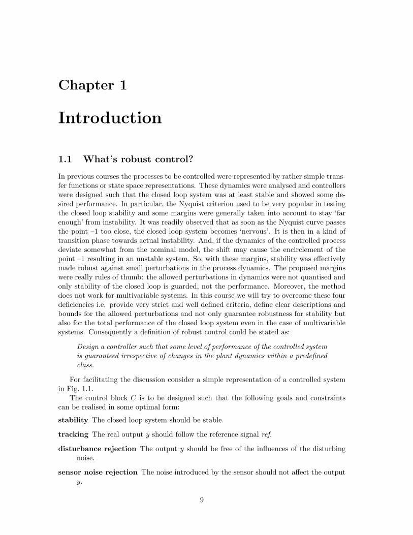
For facilitating the discussion consider a simple representation of a controlled systemin Fig. 1.1.
The control block C is to be designed such that the following goals and constraintscan be realised in some optimal form:
stability The closed loop system should be stable.
tracking The real output y should follow the reference signal ref.
disturbance rejection The output y should be free of the influences of the disturbingnoise.
sensor noise rejection The noise introduced by the sensor should not affect the outputy.
9
10 CHAPTER 1. INTRODUCTION
Figure 1.1: Simple block scheme of a controlled system
avoidence of actuator saturation The actuator, not explicitly drawn here but takenas the first part of process P , should not become saturated but has to operate as alinear transfer.
robustness If the real dynamics of the process change by an amount ∆P , the per-formance of the system, i.e. all previous desiderata, should not deteriorate to anunacceptable level. (In specific cases it may be that only stability is considered.)
It will be clear that all above desiderata can only be fulfilled to some extent. It will beexplained how some constraints put similar demands on the controller C, while othersrequire contradictory actions, and as a result the final controller can only be a kind ofcompromise. To that purpose it is important that we can quantify the various aimsand consequently weight each claim against the others. As an example, emphasis on therobustness requirement weakens the other achievable constraints, because a performanceshould not only hold for a very specific process P , where the control action can be tunedvery specifically, but also for deviating dynamics. The true process dynamics are thengiven by:
Ptrue = P + ∆P (1.1)
where now P takes the role of the nominal model while ∆P represents the additivemodel perturbation. Their is no way to avoid ∆P considering the causes behind it:
unmodelled dynamics The nominal model P will generally be taken linear, time-invariantand of low order. As a consequence the real behaviour is necessarily approximated,since real processes cannot be caught in those simple representations.
time variance Inevitably the real dynamics of physical processes change in time. Theyare susceptable to wear during aging (e.g. steel rollers), will be affected by pollution(e.g. catalysts) or undergo the influence of temperature (or pressure, humidity . . . )changes (e.g. day and night fluctuations in glass furnaces).
varying loads Dynamics can substantially change, if the load is altered: the mass andthe inertial moment of a robot arm is determined considerably by the load unlessyou are willing to pay for a very heavy robot that is very costly in operation.
manufacturing variance A prototype process may be characterised very accurately.This is of no help, if the variance over the production series is high. A low varianceproduction can turn to be immensely costly, if one thinks e.g. of a CD-player.Basically, one can produce a drive with tolerances in the micrometer-domain but,thanks to control, we can be satisfied with less.
1.2. H∞ IN A NUTSHELL 11
limited identification Even if the real process were linear and time-invariant, we stillhave to measure or identify its characteristics and this cannot be done without anerror. Measuring equipment and identification methods, using finite data sets oflimited sample rate, will inevitably be suffering from inaccuracies.
actuators & sensors What has been said about the process can be attributed to actu-ators and sensors as well, that are part of the controlled system. One might requirea minimum level of performance (e.g. stability) of the controlled system in case ofe.g. sensor failure or actuator degradation.
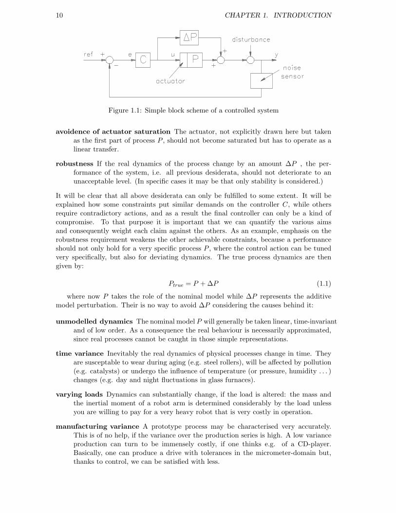
In Fig. 1.2 the effect of the robustness requirement is illustrated.
Figure 1.2: Robust performance
In concedance to the natural inclination to consider something as being ”better” ifit is ”higher”, optimal performance is a maximum here. This is contrary to the criteria,to be introduced later on, where the best performance occurs in the minimum. So herethe vertical axis represents a degree of performance where higher value indicate betterperformance. Positive values are representing improvements by the control action com-pared to the uncontrolled situation and negative values correspond to deteriorations bythe very use of the controller. For extreme values −∞ the system is unstable and +∞ isthe extreme optimist’s performance. In this supersimplified picture we let the horizontalaxis represent all possible plant behaviours centered around the nominal plant P with adeviation ∆P living in the shaded slice. So this slice represents the class of possible plants.If the controller is designed to perform well for just the nominal process, it can really befine-tuned to it, but for a small model error ∆P the performance will soon deterioratedramatically. We can improve this effect by robustifying the control and indeed improvethe performance for greater ∆P but unfortunately and inevitably at the cost of the per-formance for the nominal model P . One will readily recognise this effect in many technicaldesigns (cars,bikes,tools,. . . ), but also e.g. in natural evolution (animals, organs,. . . ).
1.2 H∞ in a nutshell
The techniques, to be presented in this course, are namedH∞-control and µ -analysis/synthesis.They have been developped since the beginning of the eighties and are, as a matter of fact,a well quantised application of the classical control design methods, fully applied in thefrequency domain. It thus took about forty years to evolve a mathematical context strong
12 CHAPTER 1. INTRODUCTION
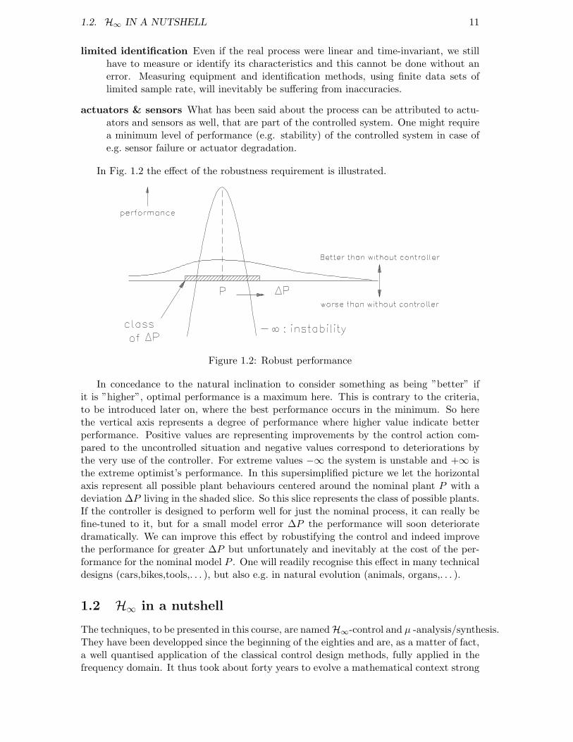
enough to tackle this problem. However, the intermediate popularity and evolution of theLQG-design in time domain was not in vain, as we will elucidate in the next chapter 2 andin the discussion of the final solution in chapters 11 and 13. It will then follow that LQGis just one alternative in a very broad set of possible robust controllers each characterisedby their own signal and system spaces. This may appear very abstract at the moment butthese normed spaces are necessary to quantify signals and transfer functions in order tobe able to compare and weight the various control goals. The definitions of the variousnormed spaces are given in chapter 5 while the translation of the various control goals isdescribed in detail in chapter 3. Here we will shortly outline the whole procedure startingwith a rearrangment in Fig.1.3 of the structure of the problem in Fig.1.1.
C P
∆P
d
r
η
+
+
+
− +
+
+
+
+
−
u
z
e y
inputs
outputs
Figure 1.3: Structure dictated by exogenous inputs and outputs to be minimised
On the left we have gathered all inputs of the final closed loop system that we do notknow beforehand but that will live in certain bounded sets. These so called exogenousinputs consist in this case of the reference signal r,the disturbance d and the measurementnoise η. These signals will be characterised as bounded by a (mathematical) ball of radius 1in a normed space together with filters that represent their frequency contents as discussedin chapter 5. Next, at the right side we have put together those output signals that haveto be minimised according to the control goals in a similar characterisation as the inputsignals. We are not interested in minimising the actual output y (so this is not part ofthe output) but only in the way that y follows the reference signal r. Consequently theerror z = r − y is taken as an output to be minimised. Note also that we have takenthe difference with the actual y and not the measured error e. As an extra output to beminimised is shown the input u of the real process in order to avoid actuator saturation.How strong this constraint is in comparison to the tracking aim depends on the qualityand thus price of the actuator and is going to be translated in forthcoming weightingsand filters. Another goal, i.e. the attenuation of effects of both the disturbance d and themeasurement noise η is automatically represented by the minimisation of output z. In amore complicated way also the effect of perturbation ∆P on the robustness of stabilityand performance should be minimised. As is clearly observed from Fig.1.3 ∆P is an extratransfer between output u and input d . If we can keep the transfer from d to u small by aproper controller, the loop closed by ∆P won’t have much effect. Consequently robustnessis increased implicitely by keeping u small as we will analyse in chapter 3. Therefor we

1.2. H∞ IN A NUTSHELL 13
have to quantify the bounds of ∆P again by a proper ball or norm and filters.At last we have to provide a linear, time-invariant, nominal model P of the dynamics
of the process that may be a multivariable (MIMO Multi Input Multi Input) transfer.In the multivariable case all single lines then represent vectors of signals. Provisionallywe will discuss the matter in s-domain so that P is representing a transfer function ins-domain. In the multivariable case, P is a transfer matrix where each entry is a transferfunction of the corresponding input to the corresponding output. The same holds for thecontroller C and consequently the signals (lines) represent vectors in s-domain so that wecan write e.g. u(s) = C(s)e(s). Having characterised the control goals in terms of outputsto be minimised provided that the inputs remain confined as defined, the principle ideabehind the control design of block C now consists of three phases as presented in chapter11:
1. Compute a controller C0 that stabilises P .
2. Establish around this central controller C0 the set of all controllers that stabilise Paccording to the Youla parametrisation.
3. Search in this last set for that (robust) controller that minimises the outputs in theproper sense.
This design procedure is quite unusual at first instance so that we start to analyse it forstable transfers P where we can apply the internal model approach in chapter 4. After-wards the original concept of a general solution is given in chapter 11. This historicallyfirst method is treated as it shows a clear analysis of the problem. In later times improvedsolution algorithms have been developped by means of Riccati equations or by means ofLinear Matrix Inequalities (LMI) as explained in Chapter 13. In the next chapter 8 therobustness concept will be revisited and improved which will yield the µ-analysis/synthesis.
After the theory, which is treated till here, chapter 9 is devoted to the selection ofappropriate design filters in practice, while in the last chapter 10 an example illustratesthe methods, algorithms and programs. In this chapter you will also get instructions howto use dedicated toolboxes in MATLAB.
14 CHAPTER 1. INTRODUCTION
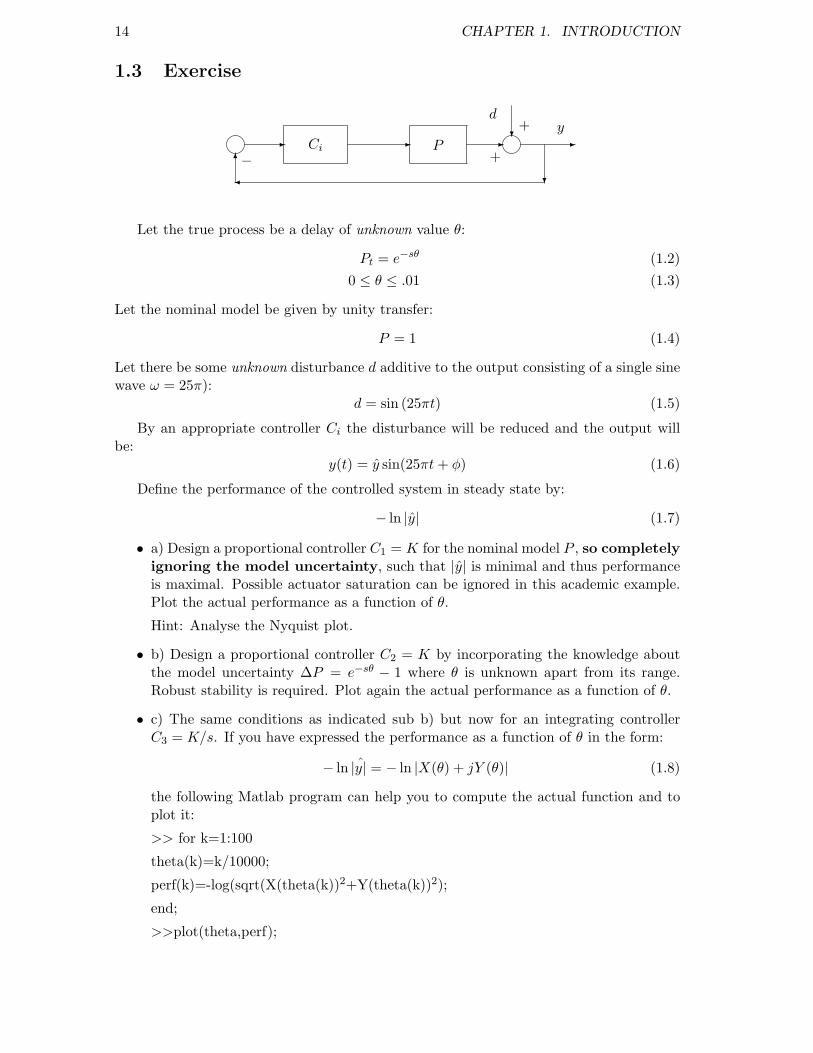
1.3 Exercise
PCi
−
dy+
+
Let the true process be a delay of unknown value θ:
Pt = e−sθ (1.2)0 ≤ θ ≤ .01 (1.3)
Let the nominal model be given by unity transfer:
P = 1 (1.4)
Let there be some unknown disturbance d additive to the output consisting of a single sinewave ω = 25π):
d = sin (25πt) (1.5)
By an appropriate controller Ci the disturbance will be reduced and the output willbe:
y(t) = y sin(25πt+ φ) (1.6)
Define the performance of the controlled system in steady state by:
− ln |y| (1.7)
• a) Design a proportional controller C1 = K for the nominal model P , so completelyignoring the model uncertainty, such that |y| is minimal and thus performanceis maximal. Possible actuator saturation can be ignored in this academic example.Plot the actual performance as a function of θ.
Hint: Analyse the Nyquist plot.
• b) Design a proportional controller C2 = K by incorporating the knowledge aboutthe model uncertainty ∆P = e−sθ − 1 where θ is unknown apart from its range.Robust stability is required. Plot again the actual performance as a function of θ.
• c) The same conditions as indicated sub b) but now for an integrating controllerC3 = K/s. If you have expressed the performance as a function of θ in the form:
− ln |y| = − ln |X(θ) + jY (θ)| (1.8)
the following Matlab program can help you to compute the actual function and toplot it:
>> for k=1:100
theta(k)=k/10000;
perf(k)=-log(sqrt(X(theta(k))2+Y(theta(k))2);
end;
>>plot(theta,perf);
Chapter 2
What about LQG?
K
A
1sI CB
−L
At
1sI CtBt
u
y
v w
x
x
++
+
+
++
+−
++
e
plant
controller
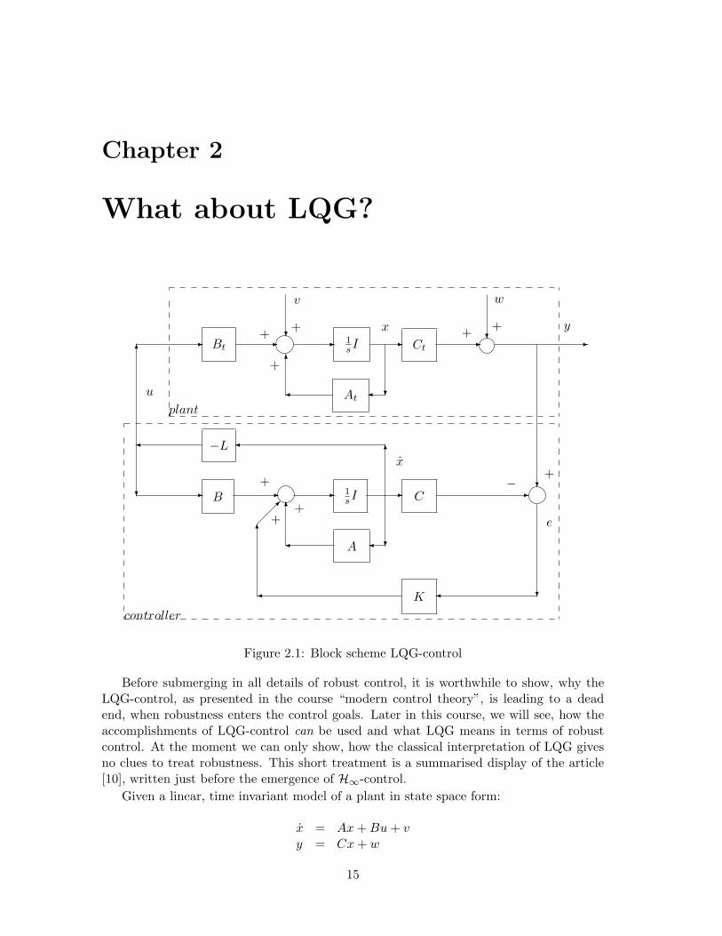
Figure 2.1: Block scheme LQG-control
Before submerging in all details of robust control, it is worthwhile to show, why theLQG-control, as presented in the course “modern control theory”, is leading to a deadend, when robustness enters the control goals. Later in this course, we will see, how theaccomplishments of LQG-control can be used and what LQG means in terms of robustcontrol. At the moment we can only show, how the classical interpretation of LQG givesno clues to treat robustness. This short treatment is a summarised display of the article[10], written just before the emergence of H∞-control.
Given a linear, time invariant model of a plant in state space form:
x = Ax+Bu+ vy = Cx+ w
15
16 CHAPTER 2. WHAT ABOUT LQG?
where u is the control input, y is the measured output, x is the state vector, v is the statedisturbance and w is the measurement noise. This multivariable process is assumed to becompletely detectable and reachable. Fig. 2.1 intends to recapitulate the set-up of theLQG-control, where the state feedback matrix L and the Kalman gain K are obtainedfrom the well known citeria to be minimised:
L = arg minExTQx+ uTRu (2.1)K = arg minE(x− x)T (x− x) (2.2)
for nonnegative Q and positive definite R. Certainly, the closed loop LQG-scheme isnominally stable, but the crucial question is, whether stability is possibly lost, if the realsystem, represented by state space matrices At, Bt, Ct, does no longer correspond to themodel of the form A,B,C. The robust stability, which is then under study, can best beillustrated by a numerical example .
Consider a very ordinary, stable and minimum phase transfer function:
P (s) =s+ 2
(s+ 1)(s+ 3)(2.3)
which admits the following state space representation:
x =(
0 1−3 −4
)x+
(01
)u+ v
y =(
2 1)x+ w
(2.4)
where v and w are independent white noise sources of variances:
Ew2 = 1 , EvvT =(
1225 −2135−2135 3721
)(2.5)
and the control criterion given by:
ExT
(2800 80
√35
80√
35 80
)x+ u2 (2.6)
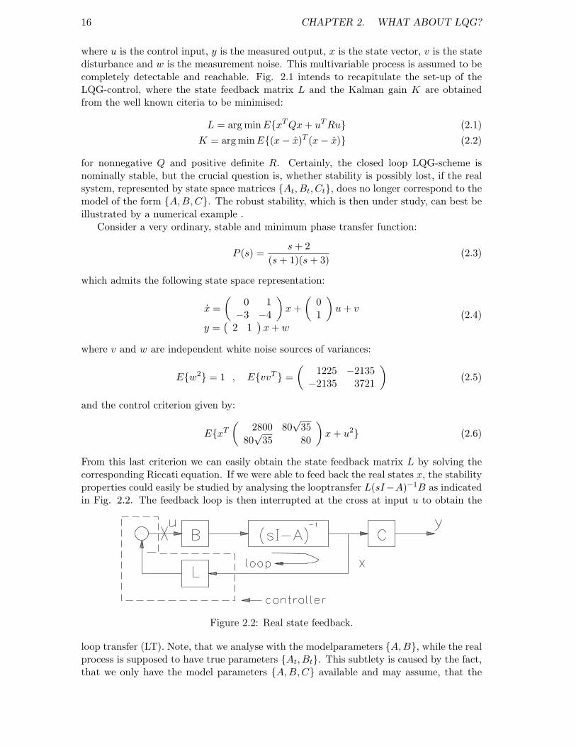
From this last criterion we can easily obtain the state feedback matrix L by solving thecorresponding Riccati equation. If we were able to feed back the real states x, the stabilityproperties could easily be studied by analysing the looptransfer L(sI−A)−1B as indicatedin Fig. 2.2. The feedback loop is then interrupted at the cross at input u to obtain the
Figure 2.2: Real state feedback.
loop transfer (LT). Note, that we analyse with the modelparameters A,B, while the realprocess is supposed to have true parameters At, Bt. This subtlety is caused by the fact,that we only have the model parameters A,B,C available and may assume, that the
17
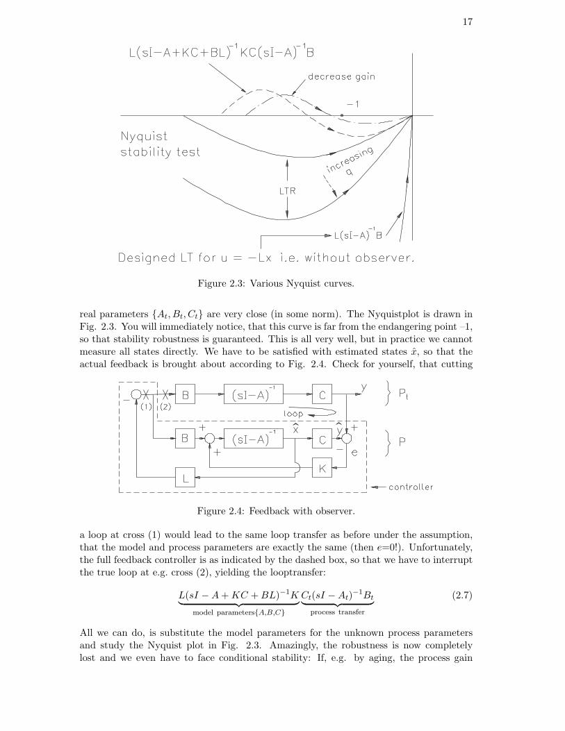
Figure 2.3: Various Nyquist curves.
real parameters At, Bt, Ct are very close (in some norm). The Nyquistplot is drawn inFig. 2.3. You will immediately notice, that this curve is far from the endangering point –1,so that stability robustness is guaranteed. This is all very well, but in practice we cannotmeasure all states directly. We have to be satisfied with estimated states x, so that theactual feedback is brought about according to Fig. 2.4. Check for yourself, that cutting
Figure 2.4: Feedback with observer.
a loop at cross (1) would lead to the same loop transfer as before under the assumption,that the model and process parameters are exactly the same (then e=0!). Unfortunately,the full feedback controller is as indicated by the dashed box, so that we have to interruptthe true loop at e.g. cross (2), yielding the looptransfer:
L(sI −A+KC +BL)−1K︸ ︷︷ ︸model parametersA,B,C
Ct(sI −At)−1Bt︸ ︷︷ ︸process transfer
(2.7)
All we can do, is substitute the model parameters for the unknown process parametersand study the Nyquist plot in Fig. 2.3. Amazingly, the robustness is now completelylost and we even have to face conditional stability: If, e.g. by aging, the process gain
18 CHAPTER 2. WHAT ABOUT LQG?
decreases, the Nyquist curve shrinks to the origin and soon the point –1 is tresspassed,causing instability.
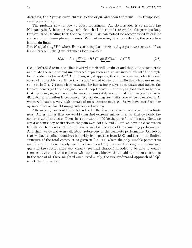
The problem now is, how to effect robustness. An obvious idea is to modify theKalman gain K in some way, such that the loop transfer resembles the previous looptransfer, when feeding back the real states. This can indeed be accomplished in case ofstable and minimum phase processes. Without entering into many details, the procedureis in main lines:Put K equal to qBW , where W is a nonsingular matrix and q a positive constant. If welet q increase in the (thus obtained) loop transfer:
L(sI −A+ qBWC︸ ︷︷ ︸+BL)−1 qBWC︸ ︷︷ ︸(sI −A)−1B (2.8)
the underbraced term in the first inverted matrix will dominate and thus almost completelyannihilate the same second underbraced expression and we are indeed left with the simplelooptransfer ≈ L(sI −A)−1B. In doing so , it appears, that some observer poles (the realcause of the problem) shift to the zeros of P and cancel out, while the others are movedto −∞. In Fig. 2.3 some loop transfers for increasing q have been drawn and indeed thetransfer converges to the original robust loop transfer. However, all that matters here is,that, by doing so, we have implemented a completely nonoptimal Kalman gain as far asdisturbance reduction is concerned. We are dealing now with very extreme entries in Kwhich will cause a very high impact of measurement noise w. So we have sacrificed ouroptimal observer for obtaining sufficient robustness.
Alternatively, we could have taken the feedback matrix L as a means to effect robust-ness. Along similar lines we would then find extreme entries in L, so that certainly theactuator would saturate. Then this saturation would be the price for robustness. Next, wecould of course try to distribute the pain over both K and L, but we have no clear meansto balance the increase of the robustness and the decrease of the remaining performance.And then, we do not even talk about robustness of the complete performance. On top ofthat we have confined ourselves implicitly by departing from LQG and thus to the limitedstructure of the total controller as given in Fig. 2.1, where the only tunable parametersare K and L. Conclusively, we thus have to admit, that we first ought to define andquantify the control aims very clearly (see next chapter) in order to be able to weightthem relatively and then come up with some machinary, that is able to design controllersin the face of all these weighted aims. And surely, the straightforward approach of LQGis not the proper way.

2.1. EXERCISE 19
2.1 Exercise
Above block scheme represents a process P of first order disturbed by white state noisev and independent white measurement noise w. L is the state feedback gain. K is theKalman observer gain based upon the known variances of v and w.
• a) If we do not penalise the control signal u, what would be the optimal L? Couldthis be allowed here?
• b) Suppose that for this L the actuator is not saturated. Is the resultant controllerC robust (in stability)? Is it satisfying the 450 phase margin?
• c) Consider the same questions when P = 1s(s+1) and in particular analyse what you
have to compute and how.(Do not try to actually do the computations.) What canyou do if the resultant solution is not robust?

20 CHAPTER 2. WHAT ABOUT LQG?
Chapter 3
Control goals
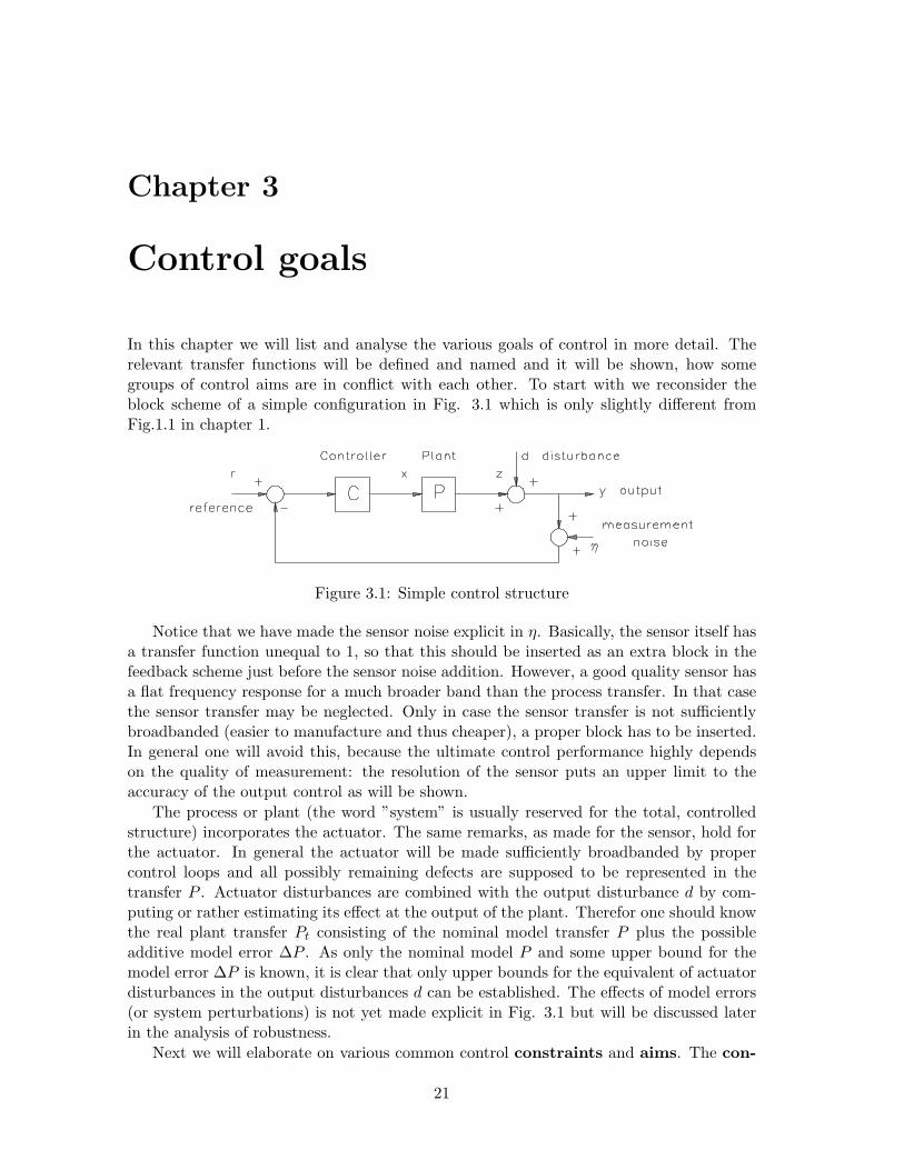
In this chapter we will list and analyse the various goals of control in more detail. Therelevant transfer functions will be defined and named and it will be shown, how somegroups of control aims are in conflict with each other. To start with we reconsider theblock scheme of a simple configuration in Fig. 3.1 which is only slightly different fromFig.1.1 in chapter 1.
Figure 3.1: Simple control structure
Notice that we have made the sensor noise explicit in η. Basically, the sensor itself hasa transfer function unequal to 1, so that this should be inserted as an extra block in thefeedback scheme just before the sensor noise addition. However, a good quality sensor hasa flat frequency response for a much broader band than the process transfer. In that casethe sensor transfer may be neglected. Only in case the sensor transfer is not sufficientlybroadbanded (easier to manufacture and thus cheaper), a proper block has to be inserted.In general one will avoid this, because the ultimate control performance highly dependson the quality of measurement: the resolution of the sensor puts an upper limit to theaccuracy of the output control as will be shown.
The process or plant (the word ”system” is usually reserved for the total, controlledstructure) incorporates the actuator. The same remarks, as made for the sensor, hold forthe actuator. In general the actuator will be made sufficiently broadbanded by propercontrol loops and all possibly remaining defects are supposed to be represented in thetransfer P . Actuator disturbances are combined with the output disturbance d by com-puting or rather estimating its effect at the output of the plant. Therefor one should knowthe real plant transfer Pt consisting of the nominal model transfer P plus the possibleadditive model error ∆P . As only the nominal model P and some upper bound for themodel error ∆P is known, it is clear that only upper bounds for the equivalent of actuatordisturbances in the output disturbances d can be established. The effects of model errors(or system perturbations) is not yet made explicit in Fig. 3.1 but will be discussed laterin the analysis of robustness.
Next we will elaborate on various common control constraints and aims. The con-
21

22 CHAPTER 3. CONTROL GOALS
straints can be listed as stability, robust stability and (avoidance of) actuator saturation.Within the freedom, left by these constraints, one wants to optimise, in a weighted balance,aims like disturbance reduction and good tracking without introducing too much effects ofthe sensor noise and keeping this total performance on a sufficient level in the face of thesystem perturbations i.e. performance robustness against model errors. In detail:
3.1 Stability.
Unless one is designing oscillators or systems in transition, the closed loop system isrequired to be stable. This can be obtained by claiming that, nowhere in the closed loopsystem, some finite disturbance can cause other signals in the loop to grow to infinity: theso-called BIBO-stability from Bounded Input to Bounded Output. Ergo all correspondingtransfers have to be checked on possible unstable poles. So certainly the straight transferbetween the reference input r and the output y, given by :
y = PC(I + PC)−1r (3.1)
But this alone is not sufficient as, in the computation of this transfer, possibly unstablepoles may vanish in a pole-zero cancellation. Another possible input position of straysignals can be found at the actual input of the plant, additive to what is indicated as x(think e.g. of drift of integrators). Let us define it by dx. Then also the transfer of dx tosay y has to be checked for stability which transfer is given by:
y = (I + PC)−1Pdx = P (I + CP )−1dx (3.2)
Consequently for this simple scheme we distinguish four different transfers from r and dx
to y and x, because a closer look soon reveals that inputs d and η are equivalent to r andoutputs z and u are equivalent to y.
3.2 Disturbance reduction.
Without feedback the disturbance d is fully present in the real output y. By means of thefeedback the effect of the disturbance can be influenced and at least be reduced in somefrequency band. The closed loop effect can be easily computed as read from:
y = PC(I + PC)−1(r − η) + (I + PC)−1︸ ︷︷ ︸S
d (3.3)
The underbraced expression represents the Sensitivity S of the output to the disturbancethus defined by:
S = (I + PC)−1 (3.4)
If we want to decrease the effect of the disturbance d on the output y, we thus have tochoose controller C such that the sensitivity S is small in the frequency band where d hasmost of its power or where the disturbance is most “disturbing”.
3.3 Tracking.
Especially for servo controllers, but in fact for all systems where a reference signal isinvolved, there is the aim of letting the output track the reference signal with a small

3.4. SENSOR NOISE AVOIDANCE. 23
error at least in some tracking band. Let us define the tracking error e in our simplesystem by:
edef= r − y = (I + PC)−1︸ ︷︷ ︸
S
(r − d) + PC(I + PC)−1︸ ︷︷ ︸T
η (3.5)
Note that e is the real tracking error and not the measured tracking error observed assignal u in Fig. 3.1, because the last one incorporates the effect of the measurementnoise substantially differently. In equation 3.5 we recognise (underbraced) the sensitivityas relating the tracking error to both the disturbance and the reference signal r. It istherefore also called awkwardly the “inverse return difference operator”. Whatever thename, it is clear that we have to keep S small in both the disturbance and the trackingband.
3.4 Sensor noise avoidance.
Without any feedback it is clear that the sensor noise will not have any influence on the realoutput y. On the other hand the greater the feedback the greater its effect in disruptingthe output. So we have to watch that in our enthousiasm to decrease the sensitivity, we arenot introducing too much sensor noise effects. This actually reminiscences to the optimalKalman gain. As the reference r is a completely independent signal, just compared withy in e, we may as well study the effect of η on the tracking error e in equation 3.5. Thecoefficient (relevant transfer) of η is then given by:
T = PC(I + PC)−1 (3.6)
and denoted as the complementary sensitivity T . This name is induced by the followingsimple relation that can easily be verified:
S + T = I (3.7)
and for SISO (Single Input Single Output) systems this turns into:
S + T = 1 (3.8)
This relation has a crucial and detrimental influence on the ultimate performance of thetotal control system! If we want to choose S very close to zero for reasons of disturbanceand tracking we are necessarily left with a T close to 1 which introduces the full sensornoise in the output and vice versa. Ergo optimality will be some compromise and themore because, as we will see, some aims relate to S and others to T .
3.5 Actuator saturation avoidance.
The input signal of the actuator is indicated by x in Fig. 3.1 because the actuator wasthought to be incorporated into the plant transfer P . This signal x should be restrictedto the input range of the actuator to avoid saturation. Its relation to all exogenous inputsis simply derived as:
x = (I + CP )−1C(r − η − d) = C(I + PC)−1︸ ︷︷ ︸R
(r − η − d) (3.9)

24 CHAPTER 3. CONTROL GOALS
The relevant (underbraced) transfer is named control sensitivity for obvious reasons andsymbolised by R thus:
R = C(I + PC)−1 (3.10)
In order to keep x small enough we have to make sure that the control sensitivity R is smallin the bands of r, η and d. Of course with proper relative weightings and “small” still tobe defined. Notice also that R is very similar to T apart from the extra multiplication byP in T . We will interprete later that this P then functions as an weighting that cannot beinfluenced by C as P is fixed. So R can be seen as a weighted T and as such the actuatorsaturation claim opposes the other aims related to S. Also in LQG-design we have metthis contradiction in a more two-faced disguise:
• Actuator saturation was prevented by proper choice of the weights R and Q in thedesign of the state feedback for disturbance reduction.
• The effect of the measurement noise was properly outweighted in the observer design.
Also the stability was stated in LQG, but its robustness and the robustness of the totalperformance was lacking and hard to introduce. In this H∞- context this comes quitenaturally as follows:
3.6 Robust stability.
Robustness of the stability in the face of model errors will be treated here rather shortlyas more details will follow in chapter 5. The whole concept is based on the so-calledsmall gain theorem which trivially applies to the situation sketched in Fig. 3.2 . The
Figure 3.2: Closed loop with loop transfer H.
stable transfer H represents the total looptransfer in a closed loop. If we require that themodulus (amplitude) of H is less than 1 for all frequencies it is clear from Fig. 3.3 that thepolar curve cannot encompass the point -1 and thus we know from the Nyquist criterionthat the loop will always constitute a stable system. So stability is guaranteed as long as:
Figure 3.3: Small gain stability in Nyquist space
3.6. ROBUST STABILITY. 25
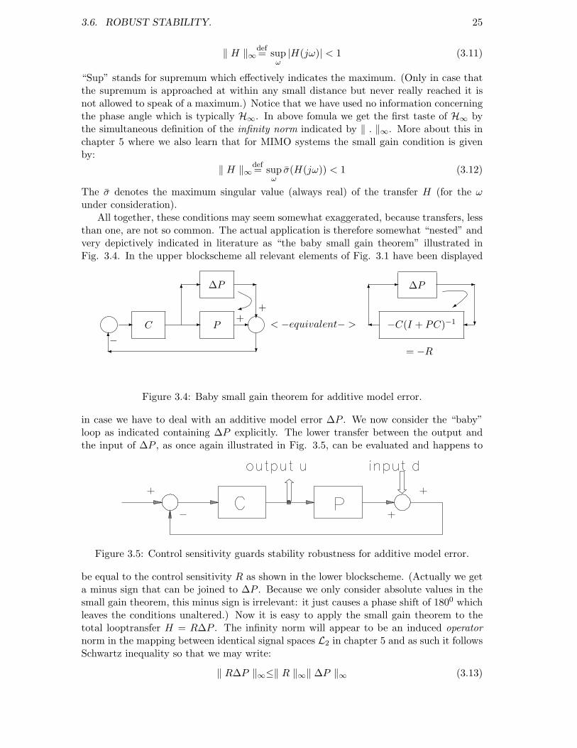
‖ H ‖∞def= supω|H(jω)| < 1 (3.11)
“Sup” stands for supremum which effectively indicates the maximum. (Only in case thatthe supremum is approached at within any small distance but never really reached it isnot allowed to speak of a maximum.) Notice that we have used no information concerningthe phase angle which is typically H∞. In above fomula we get the first taste of H∞ bythe simultaneous definition of the infinity norm indicated by ‖ . ‖∞. More about this inchapter 5 where we also learn that for MIMO systems the small gain condition is givenby:
‖ H ‖∞def= supωσ(H(jω)) < 1 (3.12)
The σ denotes the maximum singular value (always real) of the transfer H (for the ωunder consideration).
All together, these conditions may seem somewhat exaggerated, because transfers, lessthan one, are not so common. The actual application is therefore somewhat “nested” andvery depictively indicated in literature as “the baby small gain theorem” illustrated inFig. 3.4. In the upper blockscheme all relevant elements of Fig. 3.1 have been displayed
C P
∆P
−
++
∆P
= −R
< −equivalent− > −C(I + PC)−1
Figure 3.4: Baby small gain theorem for additive model error.
in case we have to deal with an additive model error ∆P . We now consider the “baby”loop as indicated containing ∆P explicitly. The lower transfer between the output andthe input of ∆P , as once again illustrated in Fig. 3.5, can be evaluated and happens to
Figure 3.5: Control sensitivity guards stability robustness for additive model error.
be equal to the control sensitivity R as shown in the lower blockscheme. (Actually we geta minus sign that can be joined to ∆P . Because we only consider absolute values in thesmall gain theorem, this minus sign is irrelevant: it just causes a phase shift of 1800 whichleaves the conditions unaltered.) Now it is easy to apply the small gain theorem to thetotal looptransfer H = R∆P . The infinity norm will appear to be an induced operatornorm in the mapping between identical signal spaces L2 in chapter 5 and as such it followsSchwartz inequality so that we may write:
‖ R∆P ‖∞≤‖ R ‖∞‖ ∆P ‖∞ (3.13)
26 CHAPTER 3. CONTROL GOALS
Ergo, if we can guarantee that:
‖ ∆P ‖∞≤ 1α
(3.14)
a sufficient condition for stability is:
‖ R ‖∞< α (3.15)
If all we require from ∆P is stated in equation 3.13 then it is easy to prove that thecondition on R is also a necessary condition. Still this is a rather crude condition but itcan be refined by weighting over the frequency axis as will be shown in chapter 5. Onceagain from Fig. 3.5 we recognise that the robustness stability constraint effectively limitsthe feedback from the point, where both the disturbance and the output of the modelerror block ∆P enter, and the input of the plant such that the loop transfer is less thanone. The smaller the error bound 1/α the greater the feedback α can be and vice versa!
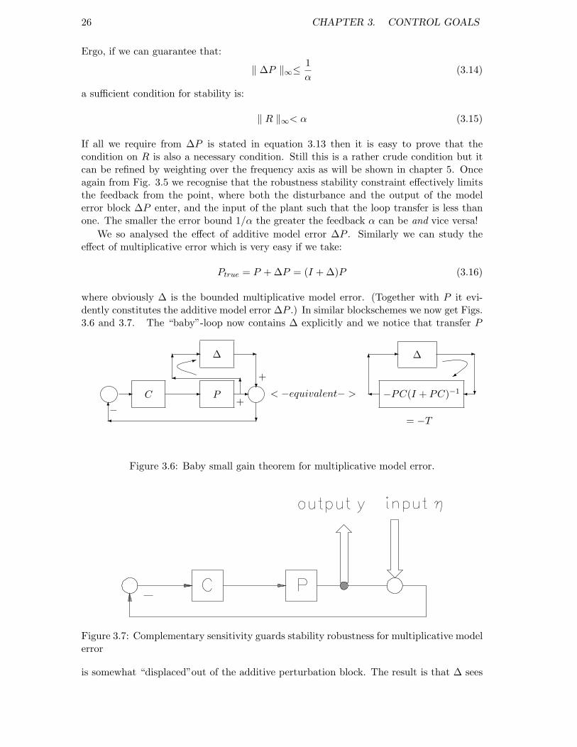
We so analysed the effect of additive model error ∆P . Similarly we can study theeffect of multiplicative error which is very easy if we take:
Ptrue = P + ∆P = (I + ∆)P (3.16)
where obviously ∆ is the bounded multiplicative model error. (Together with P it evi-dently constitutes the additive model error ∆P .) In similar blockschemes we now get Figs.3.6 and 3.7. The “baby”-loop now contains ∆ explicitly and we notice that transfer P
C P
∆
−
+
∆
= −T
< −equivalent− > −PC(I + PC)−1
+
Figure 3.6: Baby small gain theorem for multiplicative model error.
Figure 3.7: Complementary sensitivity guards stability robustness for multiplicative modelerror
is somewhat “displaced”out of the additive perturbation block. The result is that ∆ sees
3.7. PERFORMANCE ROBUSTNESS. 27
itself fed back by (minus) the complementary sensitivity T . (The P has, so to speak,been taken out of ∆P and adjoined to R yielding T .) If we require that:
‖ ∆ ‖∞≤ 1β
(3.17)
the robust stability follows from:
‖ T∆ ‖∞≤‖ T ‖∞‖ ∆ ‖∞≤ 1 (3.18)
yielding as final condition:‖ T ‖∞< β (3.19)
Again proper weighting may refine the condition.
3.7 Performance robustness.
Till now, all aims could be grouped around either the sensitivity S or the complementarysensitivity T . Once we have optimised some balanced criterion in both S and T andthus obtained a nominal performance, we wish that this performance is kept more or less,irrespective of the inevitable model errors. Consequently, performance robustness requiresthat S and T change only slightly, if P is close to the true transfer Pt. We can analysethe relative errors in these quantities for SISO plants:
St − SSt
=(1 + PtC)−1 − (1 + PC)−1
(1 + PtC)−1 = (3.20)
=1 + PC − 1− PtC
1 + PC= −∆P
P
PC
1 + PC= −∆T (3.21)
and:
Tt − TTt
=PtC(1 + PtC)−1 − PC(1 + PC)−1
PtC(1 + PtC)−1 = (3.22)
=PtC − PCPtC(1 + PC)
=∆PP
P
Pt
11 + PC
≈ ∆S (3.23)
As a result we note that in order to keep the relative change in S small we have to takethe product of ∆ and T small. The smaller the error bound is, the greater a T can weafford and vice versa. But what is astonishingly is that the smaller S is and consequentlythe greater the complement T is (see equation 3.7), the less robust is this performancemeasured in S. The same story holds for the performance measured in T where therobustness depends on the complement S. This explains the remark in chapter 1 thatincrease of performance for a particular nominal model P decreases its robustness formodel errors. So also in this respect the controller will have to be a compromise!
SummaryWe can distinguish two competitive groups because S + T = I. One group centered
around the sensitivity that requires the controller C to be such that S is “small” and canbe listed as:
• disturbance rejection
• tracking
• robustness of T

28 CHAPTER 3. CONTROL GOALS
The second group centers around the complementary sensitivity and requires the controllerC to minimise T :
• avoidance of sensor noise
• avoidance of actuator saturation
• stability robustness
• robustness of S
If we were dealing with real numbers only, the choice would be very easy and limited.Remembering that
S = (I + PC)−1 (3.24)T = PC(I + PC)−1 (3.25)
a large C would imply a small S but T ≈ I while a small C would yield a small T andS ≈ I. Besides, for no feedback, i.e. C = 0, , necessarily T → 0 and S → I. Thisis also true for very large ω when all physical processes necessarily have a zero transfer(PC → 0). So ultimately for very high frequencies, the tracking error and the disturbanceeffect is inevitably 100%.
This may give some rough ideas of the effect of C, but the real impact is more difficultas:
• We deal with complex numbers .
• The transfer may be multivariable and thus we encounter matrices.
• The crucial quantities S and T involve matrix inversions (I + PC)−1
• The controller C may only be chosen from the set of stabilising controllers.
It happens that we can circumvent the last two problems, in particular when we are dealingwith a stable transfer P . This can be done by means of the internal model control conceptas shown in the next chapter. We will later generalise this for also unstable nominalprocesses.
3.8. EXERCISES 29
3.8 Exercises
3.1:
C P
r ++
–
u′
++u
d
++ y
• a) Derive by reasoning that in the above scheme internal stability is guaranteed ifall transfers from u′ and d to u and y are stable.
• b) Analyse the stability for
P =1
1− s (3.26)
C =1− s1 + s
(3.27)
3.2:
PC2
C3
C1
r +
–
d
+ + y
Which transfers in the given scheme are relevant for:
• a) disturbance reduction
• b) tracking

30 CHAPTER 3. CONTROL GOALS
Chapter 4
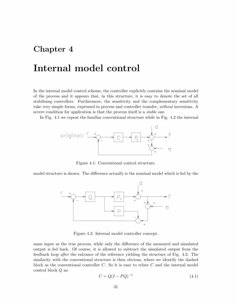
Internal model control
In the internal model control scheme, the controller explicitly contains the nominal modelof the process and it appears that, in this structure, it is easy to denote the set of allstabilising controllers. Furthermore, the sensitivity and the complementary sensitivitytake very simple forms, expressed in process and controller transfer, without inversions. Asevere condition for application is that the process itself is a stable one.
In Fig. 4.1 we repeat the familiar conventional structure while in Fig. 4.2 the internal
Figure 4.1: Conventional control structure.
model structure is shown. The difference actually is the nominal model which is fed by the
Figure 4.2: Internal model controller concept.
same input as the true process, while only the difference of the measured and simulatedoutput is fed back. Of course, it is allowed to subtract the simulated output from thefeedback loop after the entrance of the reference yielding the structure of Fig. 4.3. Thesimilarity with the conventional structure is then obvious, where we identify the dashedblock as the conventional controller C. So it is easy to relate C and the internal modelcontrol block Q as:
C = Q(I − PQ)−1 (4.1)
31
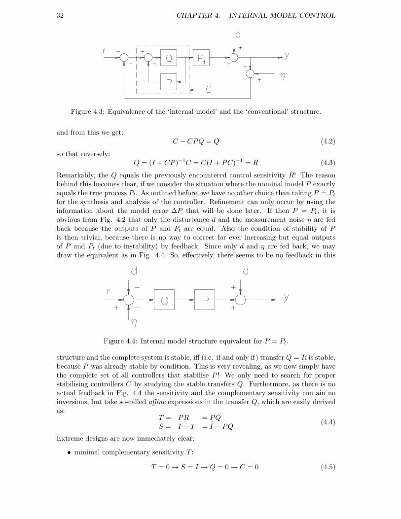
32 CHAPTER 4. INTERNAL MODEL CONTROL
Figure 4.3: Equivalence of the ‘internal model’ and the ‘conventional’ structure.
and from this we get:C − CPQ = Q (4.2)
so that reversely:Q = (I + CP )−1C = C(I + PC)−1 = R (4.3)
Remarkably, the Q equals the previously encountered control sensitivity R! The reasonbehind this becomes clear, if we consider the situation where the nominal model P exactlyequals the true process Pt. As outlined before, we have no other choice than taking P = Pt
for the synthesis and analysis of the controller. Refinement can only occur by using theinformation about the model error ∆P that will be done later. If then P = Pt, it isobvious from Fig. 4.2 that only the disturbance d and the measurement noise η are fedback because the outputs of P and Pt are equal. Also the condition of stability of Pis then trivial, because there is no way to correct for ever increasing but equal outputsof P and Pt (due to instability) by feedback. Since only d and η are fed back, we maydraw the equivalent as in Fig. 4.4. So, effectively, there seems to be no feedback in this
Figure 4.4: Internal model structure equivalent for P = Pt.
structure and the complete system is stable, iff (i.e. if and only if) transfer Q = R is stable,because P was already stable by condition. This is very revealing, as we now simply havethe complete set of all controllers that stabilise P ! We only need to search for properstabilising controllers C by studying the stable transfers Q. Furthermore, as there is noactual feedback in Fig. 4.4 the sensitivity and the complementary sensitivity contain noinversions, but take so-called affine expressions in the transfer Q, which are easily derivedas:
T = PR = PQS = I − T = I − PQ (4.4)
Extreme designs are now immediately clear:
• minimal complementary sensitivity T :
T = 0→ S = I → Q = 0→ C = 0 (4.5)
33
there is obviously neither feedback nor control causing:
– no measurement influence (T=0)
– no actuator saturation (R=Q=0)
– 100% disturbance in output (S=I)
– 100% tracking error (S = I)
– stability (Pt was stable)
– robust stability (R=Q=0 and T=0)
– robust S (T=0), but this “performance” can hardly be worse.
• minimal sensitivity S:
S = 0→ T = I → Q = P−1 → C =∞ (4.6)
if at least P−1 exists and is stable, we get infinite feedback causing:
– all disturbance is eliminated from the output (S = 0)
– y tracks r exactly (S=0)
– y is fully contaminated by measurement noise (T = I)
– stability only in case Q = P−1 is stable
– very likely actuator saturation (Q = R will tend to infinity see later)
– questionable robust stability (Q = R will tend to infinity see later)
– robust T (S = 0), but this “performance” can hardly be worse too.
Once again it is clear that a good control should be a well designed compromise betweenthe indicated extremes. What is left is to analyse the possibility of the above last sketchedextreme where we needed that PQ = I and Q is stable.
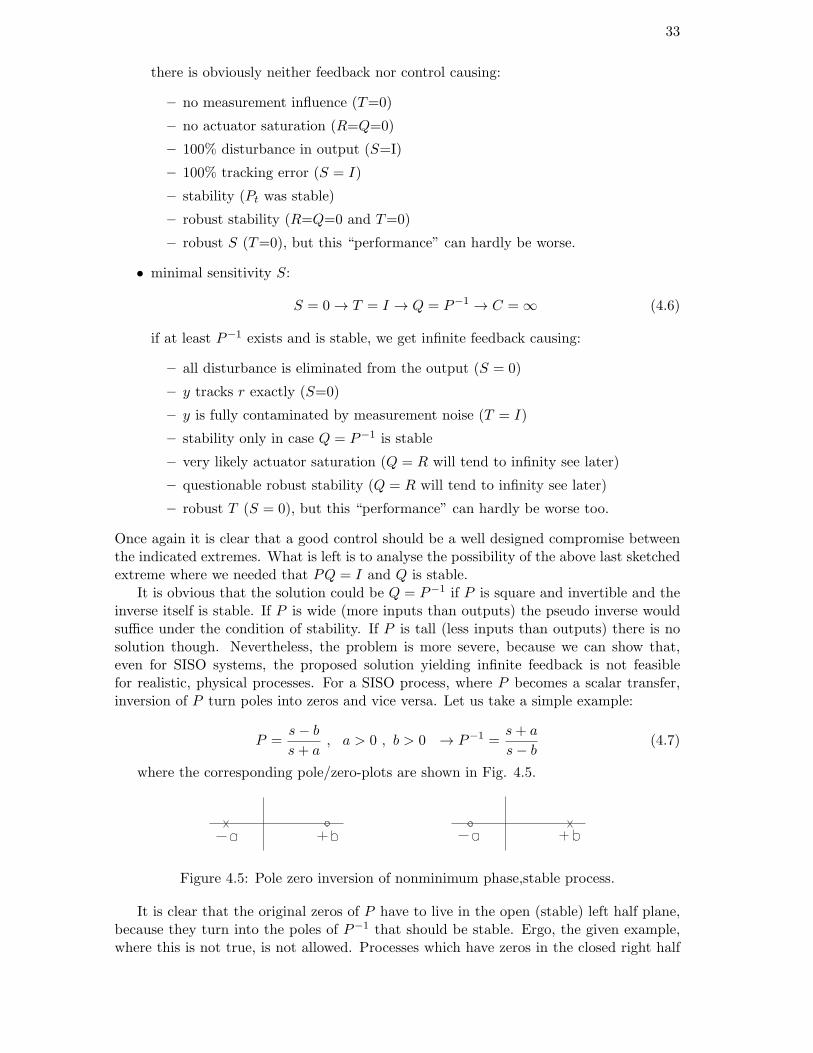
It is obvious that the solution could be Q = P−1 if P is square and invertible and theinverse itself is stable. If P is wide (more inputs than outputs) the pseudo inverse wouldsuffice under the condition of stability. If P is tall (less inputs than outputs) there is nosolution though. Nevertheless, the problem is more severe, because we can show that,even for SISO systems, the proposed solution yielding infinite feedback is not feasiblefor realistic, physical processes. For a SISO process, where P becomes a scalar transfer,inversion of P turn poles into zeros and vice versa. Let us take a simple example:
P =s− bs+ a
, a > 0 , b > 0 → P−1 =s+ a
s− b (4.7)
where the corresponding pole/zero-plots are shown in Fig. 4.5.
Figure 4.5: Pole zero inversion of nonminimum phase,stable process.
It is clear that the original zeros of P have to live in the open (stable) left half plane,because they turn into the poles of P−1 that should be stable. Ergo, the given example,where this is not true, is not allowed. Processes which have zeros in the closed right half
34 CHAPTER 4. INTERNAL MODEL CONTROL
plane, named nonminimum phase, thus cause problems in obtaining a good performancein the sense of a small S.
In fact poles and zeros in the open left half plane can easily be compensated for byQ. Also the poles in the closed right half plane cause no real problems as the rootlocifrom them in a feedback can be “drawn” over to the left plane in a feedback by puttingzeros there in the controller. The real problems are due to the nonminimum phase zerosi.e. the zeros in the closed right half plane, as we will analyse further. But before doingso, we have to state that in fact all physical plants suffer more or less from this negativeproperty.
We need some extra notion about the numbers of poles and zeros, their definition andconsiderations for realistic, physical processes. Let np denote the number of poles andsimilarly nz the number of zeros in a conventional, SISO transfer function where denomi-nator and numerator are factorised. We can then distinguish the following categories bythe attributes:
proper if np ≥ nzbiproper if np = nz
strictly proper if np > nz
nonproper if np < nz
Any physical process should be proper because nonproperness would involve:
limω→∞P (jω) =∞ (4.8)
so that the process would effectively have poles at infinity, would have an infinitelylarge transfer at infinity and would certainly start oscillating at frequency ω = ∞. Onthe other hand a real process can neither be biproper as it then should still have a finitetransfer for ω = ∞ and at that frequency the transfer is necessarily zero. Consequentlyany physical process is by nature strictly proper. But this implies that:
limω→∞P (jω) = 0 (4.9)
and thus P has effectively (at least) one zero at infinity which is in the closed righthalf space! Take for example:
P =K
s+ a, a > 0 → P−1 =
s+ a
K(4.10)
and consequently Q = P−1 cannot be realised as it is nonproper.
4.1 Maximum Modulus Principle.
The disturbing fact about nonminimum phase zeros can now be illustrated with the useof the so-called Maximum Modulus Principle which claims:
∀H ∈ H∞ :‖ H ‖∞≥ |H(s)|s∈C+ (4.11)
It says that for all stable transfers H (i.e. no poles in the right half plane denotedby C+) the maximum modulus on the imaginary axis is always greater than or equal
4.2. SUMMARY. 35
to the maximum modulus in the right half plane. We will not prove this, but facilitateits acceptance by the following concept. Imagine that the modulus of a stable transferfunction of s is represented by a rubber sheet above the s-plane. Zeros will then pinpointthe sheet to the zero, bottom level, while poles will act as infinitely high spikes lifting thesheet. Because of the strictly properness of the transfer, there is a zero at infinity, so that,in whatever direction we travel, ultimately the sheet will come to the bottom. Because ofstability there are no poles and thus spikes in the right half plane. It is obvious that sucha rubber landscape with mountains exclusively in the left half plane will gets its heightsin the right half plane only because of the mountains in the left half plane. If we cut itprecisely at the imaginary axis we will notice only valleys at the right hand side. It isalways going down at the right side and this is exactly what the principle tells.
We are now in the position to apply the maximum modulus principle to the sensitivityfunction S of a nonminimum phase SISO process P :
‖ S ‖∞= supω|S(jω)| ≥ |S(s)|s∈C+ = |1− PQ|s∈C+
s=zn︷︸︸︷= 1 (4.12)
where zn (εC+) is any nonminimum phase zero of P . As a consequence we have to acceptthat for some ω the sensitivity has to be greater than or equal to 1. For that frequencythe disturbance and the tracking errors will thus be minimally 100%! So for some bandwe will get disturbance amplification if we want to decrease it by feedback in some other(mostly lower) band. That seems to be the price. And reminding the rubber landscape,it is clear that this band, where S > 1, is the more low frequent the closer the troublingzero is to the origin of the s-plane!
By proper weighting over the frequency axis we can still optimise a solution. For anappropriate explanation of this weighting procedure we first present the intermezzo of thenext chapter about the necessary norms.
4.2 Summary.
It has been shown that internal model control can greatly facilitate the design procedure ofcontrollers. It only holds, though, for stable processes and the generalisation to unstablesystems has to wait until chapter 11. Limitations of control are recognised in the effectsof nonminimum phase zeros of the plant and in fact all physical plant suffer from these atleast at infinity.
36 CHAPTER 4. INTERNAL MODEL CONTROL
4.3 Exercises
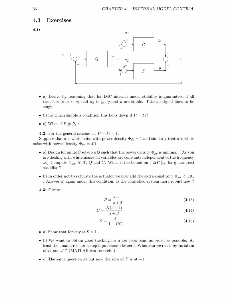
4.1:
P
Pt
Q
r +
–
u1
u2
yt
y
+
–
+
+
+
+
u
• a) Derive by reasoning that for IMC internal model stability is guaranteed if alltransfers from r, u1 and u2 to yt, y and u are stable. Take all signal lines to besingle.
• b) To which simple a condition this boils down if P = Pt?
• c) What if P = Pt ?
4.2: For the general scheme let P = Pt = 1.Suppose that d is white noise with power density Φdd = 1 and similarly that η is white
noise with power density Φηη = .01.
• a) Design for an IMC set-up a Q such that the power density Φyy is minimal. (As youare dealing with white noises all variables are constants independent of the frequencyω.) Compute Φyy, S, T , Q and C. What is the bound on ‖ ∆P ‖∞ for guaranteedstability ?
• b) In order not to saturate the actuator we now add the extra constraint Φuu < .101. Answer a) again under this condition. Is the controlled system more robust now ?
4.3: Given:
P =s− 1s+ 2
(4.13)
C =K(s+ 2)s+ β
(4.14)
S =1
1 + PC(4.15)
• a) Show that for any ω S > 1 .
• b) We want to obtain good tracking for a low pass band as broad as possible. Atleast the ‘final error’ for a step input should be zero. What can we reach by variationof K and β ? (MATLAB can be useful)
• c) The same question a) but now the zero of P is at −1.
Chapter 5
Signal spaces and norms
5.1 Introduction
In the previous chapters we defined the concepts of sensitivity and complementary sen-sitivity and we expressed the desire to keep both of these transfer functions ‘small’ in afrequency band of interest. In this chapter we will quantify in a more precise way what‘small’ means. In this chapter we will quantify the size of a signal and the size of a system.We will be rather formal to combine precise definitions with good intuition. A first sec-tion is dedicated to signals and signal norms. We then consider input-output systems anddefine the induced norm of an input-output mapping. The H∞ norm and the H2 norm ofa system are defined and interpreted both for single input single output systems, as wellas for multivariable systems.
5.2 Signals and signal norms
We will start this chapter with some system theoretic basics which will be needed in thesequel. In order to formalize concepts on the level of systems, we need to first recall somebasics on signal spaces. Many physical quantities (such as voltages, currents, temperatures,pressures) depend on time and can be interpreted as functions of time. Such functionsquantify how information evolves over time and are called signals. It is therefore logicalto specify a time set T , indicating the time instances of interest. We will think of time asa one dimensional entity and we therefore assume that T ⊆ R. We distinguish betweencontinuous time signals (T a possibly infinite interval of R) and discrete time signals (Ta countable set). Typical examples of frequently encountered time sets are finite horizondiscrete time sets T = 0, 1, 2, . . . N, infinite horizon discrete time sets T = Z+ or T = Z
or, for sampled signals, T = kτs | k ∈ Z where τs > 0 is the sampling time. Examplesof continuous time sets include T = R, T = R+ or intervals T = [a, b].
The values which a physically relevant signal assumes are usually real numbers. How-ever, complex valued signals, binary signals, nonnegative signals, angles and quantizedsignals are very common in applications, and assume values in different sets. We thereforeintroduce a signal space W , which is the set in which a signal takes its values.
Definition 5.1 A signal is a function s : T → W where T ⊆ R is the time set and W isa set, called the signal space.
More often than not, it is necessary that at each time instant t ∈ T , a number ofphysical quantities are represented. If we wish a signal s to express at instant t ∈ T a
37

38 CHAPTER 5. SIGNAL SPACES AND NORMS
total of q > 0 real valued quantities, then the signal space W consists of q copies of theset of real numbers, i.e.,
W = R× . . .× R︸ ︷︷ ︸q copies
which is denoted as W = Rq. A signal s : T → Rq thus represents at each time instantt ∈ T a vector
s(t) =
s1(t)s2(t)
...sq(t)
where si(t), the i-the component, is a real number for each time instant t.
The ‘size’ of a signal is measured by norms. Suppose that the signal space is a complexvalued q-dimensional space, i.e. W = Cq for some q > 0. We will attach to each vectorw = (w1, w2, . . . wq)′ ∈W its usual ‘length’
|w| :=√w∗
1w1 + w∗2w2 + . . .+ w∗
qwq
which is the Euclidean norm of w. (Here, w∗ denotes the complex conjugate of the complexnumber w. That is, if w = x + jy with x the real part and y the imaginary part of w,then w∗ = x − jy). If q = 1 this expresses the absolute value of w, which is the reasonfor using this notation. This norm will be attached to the signal space W , and makes ita normed space.
Signals can be classified in many ways. We distinguish between continuous and discretetime signals, deterministic and stochastic signals, periodic and a-periodic signals.
5.2.1 Periodic and a-periodic signals
Definition 5.2 Suppose that the time set T is closed under addition, that is, for any twopoints t1, t2 ∈ T also t1 + t2 ∈ T . A signal s : T →W is said to be periodic with period P(or P -periodic) if
s(t) = s(t+ P ), t ∈ T.A signal that is not P -periodic for any P is a-periodic.
Common time sets such as T = Z or T = R are closed under addition, finite time setssuch as intervals T = [a, b] are not. Well known examples of continuous time periodicsignals are sinusoidal signals s(t) = A sin(ωt+ φ) or harmonic signals s(t) = Aejωt. Here,A, ω and φ are constants referred to as the amplitude, frequency (in rad/sec) and phase,respectively. These signals have frequency ω/2π (in Hertz) and period P = 2π/ω. Weemphasize that the sum of two periodic signals does not need to be periodic. For example,s(t) = sin(t) + sin(πt) is a-periodic. The class of all periodic signals with time set T willbe denoted by P(T ).
5.2.2 Continuous time signals
It is convenient to introduce various signal classifications. First, we consider signals whichhave finite energy and finite power. To introduce these signal classes, suppose that I(t)denotes the current through a resistance R producing a voltage V (t). The instantaneouspower per Ohm is p(t) = V (t)I(t)/R = I2(t). Integrating this quantity over time, leadsto defining the total energy (in Joules). The per Ohm energy of the resistance is therefore∫∞−∞ |I(t)|2dt Joules.
5.2. SIGNALS AND SIGNAL NORMS 39
Definition 5.3 Let s be a signal defined on the time set T = R. The energy content Es
of s is defined asEs :=
∫ ∞
−∞|s(t)|2 dt
If Es <∞ then s is said to be a (finite) energy signal.
Clearly, not all signals have finite energy. Indeed, for harmonic signals s(t) = cejωt wehave that |s(t)|2 = |c|2 so that Es =∞ whenever c = 0. In general, the energy content ofperiodic signals is infinite. We therefore associate with periodic signals their power :
Definition 5.4 Let s be a continuous time periodic signal with period P . The power ofs is defined as
Ps :=1P
∫ t0+P
t0
|s(t)|2 dt (5.1)
where t0 ∈ R. If Ps <∞ then s is said to be a (finite) power signal.
In case of the resistance, the power of a (periodic) current I is measured per period andwill be in Watt. It is easily seen that the power is independent of the initial time instant t0in (5.1). A signal which is periodic with period P is also periodic with period nP , wheren is an integer. However, it is a simple exercise to verify that the right hand side of (5.1)does not change if P is replaced by nP . It is in this sense that the power is independent ofthe period of the signal. We emphasize that all nonzero finite power signals have infiniteenergy.
Example 5.5 The sinusoidal signal s(t) = A sin(ωt+φ) is periodic with period P = 2π/ω,has infinite energy and has power
Ps =ω
2π
∫ π/ω
−π/ωA2 sin2(ωt+ φ) dt =
A2
2π
∫ π
−πsin2(τ + φ) dτ = A2/2.
Let s : T → Rq be a continuous time signal. The most important norms associatedwith s are the infinity-norm, the two-norm and the one-norm defined either over a finiteor an infinite interval T . They are defined as follows
‖ s ‖∞ = maxi
supt∈T|si(t)| (5.2)
‖ s ‖2 =∫
t∈T|s(t)|2dt
1/2(5.3)
‖ s ‖1 =∫
t∈T|s(t)|dt (5.4)
More generally, the p-norm, with 1 ≤ p <∞, for continuous time signals is defined as
‖ s ‖p =∫
t∈T|s(t)|p
1/p.
Note that these quantities are defined for finite or infinite time sets T . In particular, ifT = R, ‖s‖22 = Es, i.e the energy content of a signal is the same as the square of its2-norm.
Remark 5.6 To be precise, one needs to check whether these quantities indeed definenorms. Recall from your very first course of linear algebra that a norm is defined as areal-valued function which assigns to each element s of a vector space a real number ‖ s ‖,called the norm of s, with the properties that
40 CHAPTER 5. SIGNAL SPACES AND NORMS
1. ‖ s ‖ ≥ 0 and ‖ s ‖= 0 if and only if s = 0.
2. ‖ s1 + s2 ‖ ≤ ‖ s1 ‖ + ‖ s2 ‖ for all s1 and s2.
3. ‖ αs ‖= |α| ‖ s ‖ for all α ∈ C.
The quantities defined by ‖ s ‖∞, ‖ s ‖2 and ‖ s ‖1 indeed define (signal) norms and havethe properties 1,2 and 3 of a norm.
Example 5.7 The sinusoidal signal s(t) := A sin(ωt + φ) for t ≥ 0 has finite amplitude‖ s ‖∞= A but its two-norm and one-norm are infinite.
Example 5.8 As another example, consider the signal s(t) which is described by thedifferential equations
dx
dt= Ax(t);
s(t) = Cx(t)(5.5)
where A and C are real matrices of dimension n× n and 1× n, resp. It is clear that s isuniquely defined by these equations once an initial condition x(0) = x0 has been specified.Then s is equal to s(t) = CeAtx0 where we take t ≥ 0. If the eigenvalues of A are in theleft-half complex plane then
‖ s ‖22 =∫ ∞
0xT
0eATtCTCeAtx0dt = xT
0Mx0
with the obvious definition for M . The matrix M has the same dimensions as A, issymmetric and is called the observability gramian of the pair (A,C). The observabilitygramian M is a solution of the equation
ATM +MA+ CTC = 0
which is the Lyapunov equation associated with the pair (A,C).
The sets of signals for which the above quantities are finite will be of special interest.Define
L∞(T ) = s : T →W | ‖ s ‖∞ < ∞L2(T ) = s : T →W | ‖ s ‖2 < ∞L1(T ) = s : T →W | ‖ s ‖1 < ∞P(T ) = s : T →W |
√Ps <∞
Then L∞(T ), L2(T ) and L1(T ) are normed linear signal spaces of continuous time signals.P is not a linear space as the sum of two periodic signals need not be periodic. We willdrop the T in the above signal spaces whenever the time set is clear from the context. Asan example, the sinusoidal signal of Example 5.7 belongs to L∞[0,∞) and P[0,∞), butnot to L2[0,∞) and neither to L1[0,∞).
For either finite or infinite time sets T , the space L2(T ) is a Hilbert space with innerproduct defined by
〈s1, s2〉 =∫
t∈TsT2 (t)s1(t) dt.
Two signals s1 and s2 are orthogonal if 〈s1, s2〉 = 0. This is a natural extension oforthogonality in Rn.
5.2. SIGNALS AND SIGNAL NORMS 41
The Fourier transforms
Let s : R→ R be a periodic signal with period P . The complex numbers
sk :=1P
∫ P/2
−P/2s(t)e−jkωtdt, k ∈ Z.
where ω = 2π/P , are called the Fourier coefficients of s and, whenever the summation∑∞k=−∞ |sk| <∞, the infinite sum
s(t) :=∞∑
k=−∞ske
jkωt (5.6)
converges for all t ∈ R. Moreover, if s is continuous1 then s(t) = s(t) for all t ∈ R.A continuous P -periodic signal can therefore be uniquely reconstructed from its Fouriercoefficients by using (5.6). The sequence sk, k ∈ Z, is called the (line) spectrum of s.Since the line spectrum uniquely determines a continuous periodic signal, properties ofthese signals can be expressed in terms of their line spectrum. Parseval taught us that thepower of a P -periodic signal s satisfies
Ps =∞∑
k=−∞|sk|2.
Similarly, for a-periodic continuous time signals s : R→ R for which the norm ‖s‖1 <∞,
s(ω) :=∫ ∞
−∞s(t)e−jωtdt, ω ∈ R. (5.7)
is a well defined function for all ω ∈ R. The function s is called the Fourier transform, thespectrum or frequency spectrum of s and gives a description of s in the frequency domainor ω-domain. There holds that
s(t) =12π
∫ ∞
−∞s(ω)ejωtdω, t ∈ R. (5.8)
which expresses that the function s can be recovered from its Fourier transform. Equa-tion (5.8) is usually referred to as the inverse Fourier transform of s. Using Parseval, itfollows that if s is an energy signal, then also s is an energy signal, and
Es =∫ ∞
−∞|s(t)|2dt =
12π
∫ ∞
−∞|s(ω)|2dω =
12πEs.
5.2.3 Discrete time signals
For discrete time signals s : T → Rq a similar classification can be set up. The mostimportant norms are defined as follows.
‖ s ‖∞ = maxi
supt∈T|si(t)| (5.9)
‖ s ‖2 =∑
t∈T
|s(t)|21/2
(5.10)
‖ s ‖1 =∑t∈T
|s(t)| (5.11)
1In fact, it suffices to assume that s is piecewise smooth, in which case s(t) = (s(t+) + s(t−))/2.
42 CHAPTER 5. SIGNAL SPACES AND NORMS
More generally, the p-norm, with 1 ≤ p <∞, for discrete time signals is defined as
‖ s ‖p =∑
t∈T
|s(t)|p1/p
.
Note that in all these cases the signal may be defined either on a finite or an infinitediscrete time set.
Example 5.9 A discrete time impulse is a signal s : Z→ R with
s(t) =
1 for t = 00 for t = 0
.
The amplitude of this signal ‖ s ‖∞= 1, its two-norm ‖ s ‖2= 1 and it is immediate thatals its one-norm ‖ s ‖1= 1.
Example 5.10 The signal s(t) := (1/2)t with finite time set T = 0, 1, 2 has amplitude‖ s ‖∞= 1, two-norm ‖ s ‖2= (
∑2t=0 |(1/2)t|2)1/2 = 1 + 1/4 + 1/16 = 21/16 and one-norm
‖ s ‖1= 1 + 1/2 + 1/4 = 7/4.
Example 5.11 The Fibonacci sequence (1, 1, 2, 3, 5, 8, 13, . . .) (got the idea?) can beviewed as a signal s : Z+ → N with s(t) the t-th element of the sequence. Note that‖ s ‖∞=‖ s ‖2=‖ s ‖1=∞ for this signal. Obviously, not all signals have finite norms.
As in the previous subsection, finite norm signals are of special interest and define thefollowing normed signal spaces
∞(T ) = s : T →W | ‖ s ‖∞ < ∞2(T ) = s : T →W | ‖ s ‖2 < ∞1(T ) = s : T →W | ‖ s ‖1 < ∞
for discrete time signals. We emphasize that these are sets of signals. Again, the argumentT will be omitted whenever the time set T is clear from the context. The discrete timeimpulse s defined in Example 5.9 thus belongs to ∞, 2 and 1. It is easily seen that anyof these signal spaces are linear normed spaces. This means that, whenever two signalss1, s2 belong to ∞ (say), then s1 + s2 and αs1 also belong to ∞ for any real number α.
5.2.4 Stochastic signals
Occasionally we consider stocastic signals in this course. We will not give a completetreatise of stochastic system theory at this place but instead recall a few concepts.Astationary stochastic process is a sequence of real random variablesu(t) where t runs oversome time set T . By definition of stationarity,its mean, µ(t) := E [u(t)] is independentof the time instant t, and the second order moment E [u(t1)u(t2)] depends only on thedifference t1 − t2. The covariance of such a process is defined by
Ru(τ) := E[(u(t+ τ)− µ)(u(t)− µ)]
where µ = µ(t) = E [u(t)] is the mean. A stochastic (stationary) process u(t) is called awhite noise process if its mean µ = E [u(t)] = 0 and if u(t1) and u(t2) are uncorrelated forall t1 = t2. Stated otherwise, the covariance of a (continuous time) white noise process
5.3. SYSTEMS AND SYSTEM NORMS 43
is Ru(τ) = σ2δ(τ). The number σ2 is called the variance. The Fourier transform of thecovariance function Ru(τ) is
Φu(ω) :=∫ ∞
−∞Ru(τ)e−jωτdτ
and is usually referred to as the power spectrum, energy spectrum or just the spectrum ofthe stochastic process u.
5.3 Systems and system norms
A system is any set S of signals. In engineering we usually study systems which have quitesome structure. It is common engineering practice to consider systems whose signals arenaturally decomposed in two independent sets: a set of input signals and a set of outputsignals. A system then specifies the relations among the input and output signals. Theserelations may be specified by transfer functions, state space representations, differentialequations or whatever mathematical expression you can think of. We find this themein almost all applications where filter and control design are used for the processing ofsignals. Input signals are typically assumed to be unrestricted. Filters are designed soas to change the frequency characteristics of the input signals. Output signals are theresponses of the system (or filter) after excitation with an input signal. For the purpose ofthis course, we exclusively consider systems in which an input-output partitioning of thesignals has already been made. In engineering applications, it is good tradition to depictinput-output systems as ‘blocks’ as in Figure 5.3, and you probably have a great dealof experience in constructing complex systems by interconnecting various systems usingblock diagrams. The arrows in Figure 5.3 indicate the causality direction.
Remark 5.12 Also a word of warning concerning the use of blocks is in its place. Forexample, many electrical networks do not have a ‘natural’ input-output partition of systemvariables, neither need such a partitioning of variables be unique. Ohm’s law V = RIimposes a simple relation among the signals ‘voltage’ V and ‘current’ I but it is notevident which signal is to be treated as input and which as output.
Hu(t) y(t)
Figure 5.1: Input-output systems: the engineering view
The mathematical analog of such a ‘block’ is a function or an operator H mappinginputs u taken from an input space U to output signals y belonging to an output space Y.We write
H : U −→ Y.
Remark 5.13 Again a philosofical warning is in its place. If an input-output system ismathematically represented as a function H, then to each input u ∈ U , H attaches aunique output y = H(u). However, more often than not, the memory structure of manyphysical systems allows various outputs to correspond to one input signal. A capacitor C
44 CHAPTER 5. SIGNAL SPACES AND NORMS
imposes the relation C ddtV = I on voltage-current pairs V, I. Taking I = 0 as input allows
the output V to be any constant signal V (t) = V0. Hence, there is no obvious mappingI → V modeling this simple relationship!
Of course, there are many ways to represent input-output mappings. We will be partic-ularly interested in (input-output) mappings defined by convolutions and those defined bytransfer functions. Undoubtedly, you have seen various of the following definitions before,but for the purpose of this course, it is of importance to understand (and fully appreciate)the system theoretic nature of the concepts below. In order not to complicate things fromthe outset, we first consider single input single output continuous time systems with timeset T = R and turn to the multivariable case in the next section. This means that we willfocus on analog systems. We will not treat discrete time (or digital) systems explicitly, fortheir definitions will be similar and apparent from the treatment below.
In a (continuous time) convolution system, an input signal u ∈ U is transformed to anoutput signal y = H(u) according to the convolution
y(t) = (Hu)(t) = (h ∗ u)(t) =∫ ∞
−∞h(t− τ)u(τ)dτ (5.12)
where h : R→ R is a function called the convolution kernel. In system theoretic language,h is usually referred to as the impulse response of the system, as the output y is equalto h whenever the input u is taken to be a Dirac impulse u(t) = δ(t). Obviously, Hdefines a linear map (as H(u1 + u2) = H(u1) +H(u2) and H(αu) = αH(u)) and for thisreason the corresponding input-output system is also called linear. Moreover, it defines atime-invariant system in the sense that H maps the time shifted input signal u(t− t0) tothe time shifted output y(t− t0).
No mapping is well defined if we are lead to guess what the domain U of H should be.There are various options:
• One can take bounded signals, i.e., U = L∞.
• One can take harmonic signals, i.e., U = cejωt | c ∈ C, ω ∈ R.• One can take energy signals, i.e., U = L2.
• One can take periodic signals with finite power, i.e., U = P.
• The input class can also exist of one signal only. If we are interested in the impulseresponse only, we take U = δ.
• One can take white noise stochastic processes as inputs. In that case U consists ofall stationary zero mean signals u with finite covariance Ru(τ) = σ2δ(τ).
Example 5.14 For example, the response to a harmonic input signal u(t) = ejωt is givenby
y(t) =∫ ∞
−∞h(τ)ejω(t−τ)dτ = h(ω)ejωt
where h is the Fourier transform of h as defined in (5.7).
Example 5.15 A P -periodic signal with line spectrum uk, k ∈ Z, can be representedas u(t) =
∑∞k=−∞ uke
jkωt where ω = 2π/P and its corresponding output is given by
y(t) =∞∑
k=−∞h(kω)uke
jkωt.
5.3. SYSTEMS AND SYSTEM NORMS 45
Consequently, y is also periodic with period P and the line spectrum of the output is givenby yk = h(kω)uk, k ∈ Z.
Assume that both U and Y are normed linear spaces. Then we call H bounded if thereis a constant M ≥ 0 such that
‖ H(u) ‖ ≤ M ‖ u ‖ .
Note that the norm on the left hand side is the norm defined on signals in the outputspace Y and the norm on the right hand side corresponds to the norm of the input signalsin U . In system theoretic terms, boundednes of H can be interpreted in the sense that His stable with respect to the chosen input class and the corresponding norms. If a linearmap H : U → Y is bounded then its norm ‖ H ‖ can be defined in several alternative(and equivalent) ways:
‖ H ‖ = infMM | ‖ Hu ‖ ≤ M ‖ u ‖, for all u ∈ U
= supu∈U ,u =0
‖ Hu ‖‖ u ‖
= supu∈U ,‖u‖≤1
‖ Hu ‖
= supu∈U ,‖u‖=1
‖ Hu ‖
(5.13)
For linear operators, all these expressions are equal and either one of them serves asdefinition for the norm of an input-output system. The norm ‖ H ‖ is often called theinduced norm or the operator norm of H and it has the interpretation of the maximal‘gain’ of the mapping H : U → Y. A most important observation is that
the norm of the input-output system defined by H depends on the class of inputsU and on the signal norms for elements u ∈ U and y ∈ Y. A different class ofinputs or different norms on the input and output signals results in differentoperator norms of H.
5.3.1 The H∞ norm of a system
Induced norms
Let T be a continuous time set. If we assume that the impulse response h : R → R
satisfies ‖ h ‖1=∫∞−∞ |h(t)|dt < ∞ (in other words, if we assume that h ∈ L1), then H is
a stable system in the sense that bounded inputs produce bounded outputs. Thus, underthis condition,
H : L∞(T ) −→ L∞(T )
and we can define the L∞-induced norm of H as
‖ H ‖(∞,∞) := supu∈L∞
‖ H(u) ‖∞‖ u ‖∞
Interestingly, under the same condition, H also defines a mapping from energy signals toenergy signals, i.e.
H : L2(T ) −→ L2(T )

46 CHAPTER 5. SIGNAL SPACES AND NORMS
with the corresponding L2-induced norm
‖ H ‖(2,2) := supu∈L2
‖ H(u) ‖2‖ u ‖2
In view of our definition of ‘energy’ signals, this norm is also referred to as the inducedenergy norm. The power does not define a norm for the class P of periodic signals.Nevertheless, Example 5.15 shows that
H : P(T )→ P(T )
and we define the power-induced norm
‖H‖pow := supPu =0
√Py√Pu
.
The following result characterizes these system norms
Theorem 5.16 Let T = R or R+ be the time set and let H be defined by (5.12). Supposethat h ∈ L1. Then
1. the L∞-induced norm of H is given by
‖ H ‖(∞,∞)=‖ h ‖1
2. the L2-induced norm of H is given by
‖ H ‖(2,2)= maxω∈R
|h(ω)| (5.14)
3. the power-induced norm of H is given by
‖ H ‖pow= maxω∈R
|h(ω)| (5.15)
We will extensively use the above characterizations of the L2-induced and power-induced norm. The first characterization on the ∞-induced norm is interesting, but willnot be further used in this course. The Fourier transform h of the impulse response h isgenerally referred to as the frequency response of the system (5.12). It has the propertythat whenever h ∈ L1 and u ∈ L2,
y(t) = (h ∗ u)(t) ⇐⇒ y(ω) = h(ω)u(ω) (5.16)
Loosely speaking, this result states that convolution in the time domain is equivalent tomultiplication in the frequency domain.
Remark 5.17 The quantity maxω∈R |h(ω)| satisfies the axioms of a norm, and is preciselyequal to the L∞-norm of the frequency response, i.e, ‖ h ‖∞= maxω∈R |h(ω)|.
Remark 5.18 The frequency response can be written as
h(ω) = |h(ω)|ejφ(ω).
Various graphical representations of frequency responses are illustrative to investigatesystem properties like bandwidth, system gains, etc. A plot of |h(ω)| and φ(ω) as function
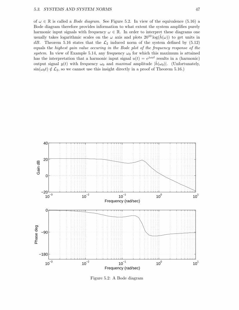
5.3. SYSTEMS AND SYSTEM NORMS 47
of ω ∈ R is called a Bode diagram. See Figure 5.2. In view of the equivalence (5.16) aBode diagram therefore provides information to what extent the system amplifies purelyharmonic input signals with frequency ω ∈ R. In order to interpret these diagrams oneusually takes logarithmic scales on the ω axis and plots 2010 log(h(ω)) to get units indB. Theorem 5.16 states that the L2 induced norm of the system defined by (5.12)equals the highest gain value occuring in the Bode plot of the frequency response of thesystem. In view of Example 5.14, any frequency ω0 for which this maximum is attainedhas the interpretation that a harmonic input signal u(t) = ejω0t results in a (harmonic)output signal y(t) with frequency ω0 and maximal amplitude |h(ω0)|. (Unfortunately,sin(ω0t) /∈ L2, so we cannot use this insight directly in a proof of Theorem 5.16.)
10−3
10−2
10−1
100
101
−20
0
20
40
Frequency (rad/sec)
Gai
n dB
10−3
10−2
10−1
100
101
−90
−180
0
Frequency (rad/sec)
Pha
se d
eg
Figure 5.2: A Bode diagram

48 CHAPTER 5. SIGNAL SPACES AND NORMS
To prove Theorem 5.16, we derive from Parseval’s identity that
‖ H ‖2(2,2) = supu∈L2
‖ h ∗ u ‖22‖ u ‖22
= supu∈L2
1/(2π) ‖ h ∗ u ‖221/(2π) ‖ u ‖22
= supu∈L2
∫ |h(ω)|2|u(ω)|2dω‖ u ‖22
≤ supu∈L2
maxω∈R |h(ω)|2 ‖ u ‖22‖ u ‖22
= maxω∈R
|h(ω)|2
which shows that ‖ H ‖(2,2) ≤ maxω∈R |h(ω)|. Similarly, using Parseval’s identity forperiodic signals
‖ H ‖2pow = supP
supu is P -periodic
Py
Pu
= supP
supu is P -periodic
∑∞k=−∞ |h(2πk/P )uk|2∑∞
k=−∞ |uk|2≤ sup
Pmaxk∈Z
|h(2πk/P )|2
= maxω∈R
|h(ω)|2
showing that ‖ H ‖pow ≤ maxω∈R |h(ω)|. Theorem 5.16 provides equality for the latterinequalities. For periodic signals (statement 3) this can be seen as follows. Suppose thatω0 is such that
|h(ω0)| = maxω∈R
|h(ω)|
Take a harmonic input u(t) = ejω0t and note that this signal has power Pu = 1 and linespectrum u1 = 1, uk = 0 for k = 1. From Example 5.14 it follows that the output y hasline spectrum y1 = h(ω0), and yk = 0 for k = 1, and using Parseval’s identity, the outputhas power Py = |h(ω0)|2. We therefore obtain that
‖ H ‖pow = h(ω0) = maxω∈R
|h(ω)|
as claimed. The proof of statement 2 is more involved and will be skipped here.
The transfer function associated with (5.12) is the Laplace transform of the impulseresponse h. This object will be denoted by H(s) (which the careful reader perceives aspoor and ambiguous notation at this stage2). Formally,
H(s) :=∫ ∞
−∞h(t)e−stdt
2For we defined H already as the mapping that associates with u ∈ U the element H(u). However,from the context it will always be clear what we mean
5.3. SYSTEMS AND SYSTEM NORMS 49
where the complex variable s is assumed to belong to an area of the complex plane wherethe above integral is finite and well defined. The Laplace transforms of signals are definedin a similar way and we have that
y = h ∗ u ⇐⇒ y(ω) = h(ω)u(ω) ⇐⇒ Y (s) = H(s)U(s).
If the Laplace transform exists in an area of the complex plane which includes the imagi-nary axis, then the Fourier transform is simply h(ω) = H(jω).
Remark 5.19 It is common engineering practice (the adjective ‘good’ or ‘bad’ is leftto your discretion) to denote Laplace transforms of signals u ambiguously by u. Thusu(t) means something really different than u(s)! Whereas y(t) = H(u)(t) refers to theconvolution (5.12), the notation y(s) = Hu(s) is to be interpreted as the product of H(s)and the Laplace transform u(s) of u(t). The notation y = Hu can therefore be interpretedin two (equivalent) ways!
We return to our discussion of induced norms. The right-hand side of (5.14) and (5.15)is defined as the H∞ norm of the system (5.12).
Definition 5.20 Let H(s) be the transfer function of a stable single input single outputsystem with frequency response h(ω). The H∞ norm of H, denoted ‖ H ‖∞ is the number
‖ H ‖∞ := maxω∈R
|h(ω)|. (5.17)
The H∞ norm of a SISO transfer function has therefore the interpretation of the maximalpeak in the Bode diagram of the frequency response h of the system and can be directly‘read’ from such a diagram. Theorem 5.16 therefore states that
‖ H(s) ‖∞=‖ H ‖(2,2)=‖ H ‖pow .
In words, this states that
the energy induced norm and the power induced norm of H is equal to the H∞norm of the transfer function H(s).

50 CHAPTER 5. SIGNAL SPACES AND NORMS
A stochastic interpretation of the H∞ norm
We conclude this subsection with a discussion on a stochastic interpretation of the H∞norm of a transfer function. Consider the set ΩT of all stochastic (continuous time)processes s(t) on the finite time interval [0, T ] for which the expectation
E‖s‖22,T := E∫ T
0sT(t)s(t) dt (5.18)
is well defined and bounded. Consider the convolution system (5.12) and assume thath ∈ L1 (i.e. the system is stable) and the input u ∈ ΩT . Then the output y is a stochasticprocess and we can introduce the “induced norm”
‖H‖2stoch,T := supu∈ΩT
E‖y‖22,T
E‖u‖22,T
which depends on the length of the time horizon T . This is closely related to an inducedoperator norm for the convolution system (5.12). We would like to extend this definitionto the infinite horizon case. For this purpose it seems reasonable to define
E‖s‖22 := limT→∞
E 1T‖s‖22,T (5.19)
assuming that the limit exists. This expectation can be interpreted as the average powerof a stochastic signal. However, as motivated in this section, we would also like to workwith input and output spaces U and Y that are linear vector spaces. Unfortunately, theclass of stochastic processes for which the limit in (5.19) exists is not a linear space. Forthis reason, the class of stochastic input signals U is set to
Ω := s | ‖s‖Ω < ∞
where
‖s‖2Ω := lim supT→∞
E 1T‖s‖22,T
In this case, Ω is a linear space of stochastic signals, but ‖ · ‖Ω does not define a normon Ω. This is easily seen as ‖s‖Ω = 0 for any s ∈ L2. However, it is a semi norm as itsatisfies conditions 2 and 3 in Remark 5.6. With this class of input signals, we can extendthe “induced norm” ‖H‖stoch,T to the infinite horizon case
‖H‖2stoch := supu∈Ω
‖y‖Ω‖u‖Ω
which is bounded for stable systems H. The following result is the crux of this discussionand states that ‖H‖stoch is, in fact, equal to the H∞ norm of the transfer function H.
Theorem 5.21 Let h ∈ L1 and let H(s) be the transfer function of the system (5.12).Then
‖H‖stoch = ‖H‖∞.A proof of this result is beyond the scope of these lecture notes. The result can be
found in [18].
5.3. SYSTEMS AND SYSTEM NORMS 51
5.3.2 The H2 norm of a system
The notation H2 is commonly used for the class of functions of a complex variable thatdo not have poles in the open right-half complex plane (they are analytic in the openright-half complex plane) and for which the norm
‖s‖H2 :=
supα>0
12π
∫ ∞
−∞s∗(α+ jω)s(α+ jω)dω
1/2
is finite. The ‘H’ stands for Hardy space. Thus,
H2 = s : C→ C | sanalytic in(s) > 0 and ‖s‖H2 <∞
. This “cold-hearted” definition has, in fact, a very elegant system theoretic interpretation.Before giving this, we first remark that the H2 norm can be evaluated on the imaginaryaxis. That is, for any s ∈ H2 one can construct a boundary function s(ω) = limα↓0 s(α+jω), which exists for almost all ω. Moreover, this boundary function is square integrable,i.e., s ∈ L2 and ‖s‖H2 = ‖s‖2. Stated otherwise,
‖s‖H2 = 1
2πs∗(ω)s(ω)
1/2
Thus, the supremum in the definition of the H2 norm always occurs on the boundaryα = 0. It is for this reason that s is usually identified with the boundary function and thebar in s is usually omitted.
Deterministic interpretation
To interpret the H norm, consider again the convolution system (5.12) and suppose thatwe are interested only in the impulse response of this system. This means, that we take theimpulse δ(t) as the only candidate input forH. The resulting output y(t) = (Hu)(t) = h(t)is an energy function so that Eh <∞. Using Parseval’s identity we obtain
Eh =‖ h ‖22=1√2π‖ h ‖22
= 1
2π
∫ ∞
−∞h∗(ω)h(ω)dω
= ‖H(s)‖2H2
where H(s) is the transfer function associated with the input-output system. The squareof the H2 norm is therefore equal to the energy of the impulse response. To summarize:
Definition 5.22 Let H(s) be the transfer function of a stable single input single outputsystem with frequency response h(ω). The H2 norm of H, denoted ‖ H ‖H2 is the number
‖ H ‖H2 := 1
2π
∫ ∞
−∞H(jω)H(−jω)dω
1/2. (5.20)
Stochastic interpretation
The H2 norm of a transfer function has an elegant equivalent interpretation in terms ofstationary stochastic signals3. The H2 norm is equal to the expected root-mean-square
3The derivations in this subsection are not relevant for the course!
52 CHAPTER 5. SIGNAL SPACES AND NORMS
(RMS) value of the output of the system when the input is a realization of a unit variancewhite noise process. That is, let
u(t) =
a unit variance white noise process t ∈ [0, T ]0 otherwise
and let y = h ∗ u be the corresponding output. Using the definition of a finite horizon2-norm from (5.18), we set
‖H‖2RMS,T := E∫ ∞
−∞yT(t)y(t)dt = E‖y‖22,T
where E denotes expectation. Substitute (5.12) in the latter expression and use thatE(u(t1)u(t2)) = δ(t1 − t2) to obtain that
‖H‖2RMS,T =∫ T
0dt
∫ t
t−Th(τ)h(τ) dτ
= T
∫ T
−Th(τ)h(τ)dτ −
∫ T
0t(h(τ)h(τ) + h(−τ)h(−tau))dτ
If the transfer function is such that the limit
‖H‖2RMS = limT→∞
1T‖H‖2RMS,T
remains bounded we obtain the infinite horizon RMS-value of the transfer function H. Infact, it then follows that
‖H‖2RMS =∫ ∞
−∞h(τ)h(τ) dτ
=12π
∫ ∞
−∞H(jω)H∗(jω) dω
= ‖H‖2H2
Thus, the H2 norm of the transfer function is equal to the infinite horizon RMS value ofthe transfer function.
Another stochastic interpretation of the H2 norm can be given as follows. Let u(t) bea stochastic process with mean 0 and covariance Ru(τ). Taking such a process as input to(5.12) results in the output y(t) which is a random variable for each time instant t ∈ T . Itis easy to see that the output y has also zero mean. The condition that h ∈ L2 guaranteesthat the output y has finite covariances Λy(τ) = E [y(t)y(t − τ)] and easy calculations4
show that the covariances Ry(τ) are given by
Ry(τ) = E [y(t+ τ)y(t)]
=∫ ∞
−∞
∫ ∞
−∞h(s′)Ru(τ + s′′ − s′)h(s′′)ds′ds′′
The latter expression is a double convolution which by taking Fourier transforms resultsin the equivalent expression
Φy(ω) = h(jω)Φu(ω)h(−jω). (5.21)4Details are not important here.
5.4. MULTIVARIABLE GENERALIZATIONS 53
in the frequency domain. We now assume u to be a white noise process with Φu(ω) = 1 forall ω ∈ R. (This implies that Ru(τ) = δ(τ). Indeed the variance of this signal theoreticallyequals ψ(0) = δ(0) = ∞. This is caused by the fact that all freqencies have equal power(density) 1, which in turn is necessary to allow for infinitely fast changes of the signalto make future values independent of momentary values irrespective of the small timedifference. Of course in practice it is sufficient if the “whiteness” is just in broadbandednoise with respect to the frequency band of the plant under study.) Using (5.21), thespectrum of the output is then given by
Φy(ω) = |h(ω)|2 (5.22)
which relates the spectrum of the input and the spectrum of the output of the systemdefined by the convloution (5.12). Integrating the latter expression over ω ∈ R and usingthe definition of the H2 norm yields that
‖ H(s) ‖2H2=
12π‖ h ‖22
=12π
∫ ∞
−∞h(ω)h(−ω)dω
=12π
∫ ∞
−∞Φy(ω)dω
= ‖ Ry(τ) ‖22
(5.23)
Thus the H2 norm of the transfer function H(s) has the interpretation of the L2 norm ofthe covariance function Ry(τ) of the output y of the system when the input u is taken tobe a white noise signal with variance equal to 1. From this it should now be evident thatwhen we define in this stochastic context the norm of a stochastic (stationary) signal swith mean 0 and covariance Rs(τ) to be
‖ s ‖ := ‖ Rs(τ) ‖2=∫ ∞
−∞E [s(t+ τ)s(t)]dτ
1/2
then the H2 norm of the transfer function H(s) is equal to the norm ‖ y ‖ of the output y,when taking white noise as input to the system. Note that above norm is rather a powernorm than an energy norm and that for a white noise input u we get
‖ u ‖=‖ Ru(τ) ‖2=∫ ∞
−∞δ(τ)dτ
1/2= 1.
5.4 Multivariable generalizations
In the previous section we introduced various norms to measure the relative size of a singleinput single output system. In this section we generalize these measures for multivariablesystems. The mathematical background and the main ideas behind the definitions andcharacterizations of norms for multivariable systems is to a large extent identical to theconcepts derived in the previous section. Throughout this section we will consider aninput-output system with m inputs and p outputs as in Figure 5.3.
Again, starting with a convolution representation of such a system, the output y isdetermined from the input u by
y(t) = (Hu)(t) = h ∗ u =∫ ∞
−∞h(t− τ)u(τ)dτ
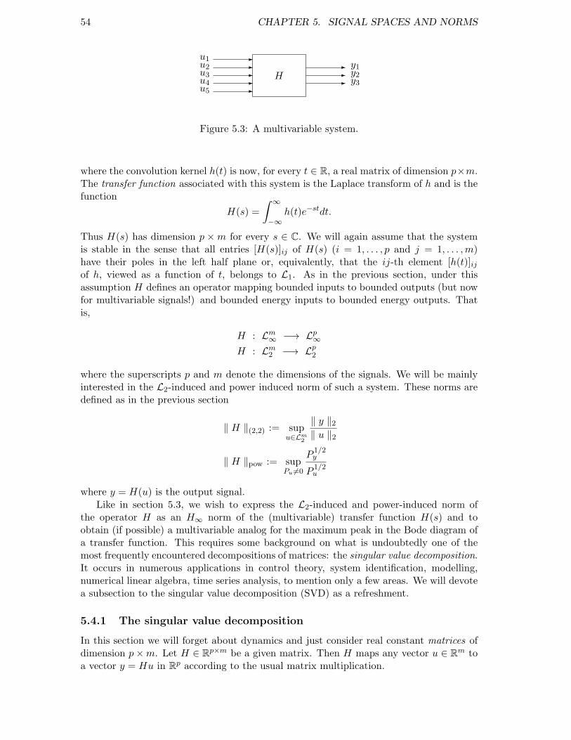
54 CHAPTER 5. SIGNAL SPACES AND NORMS
H
u5u4u3u2u1
y3y2y1
Figure 5.3: A multivariable system.
where the convolution kernel h(t) is now, for every t ∈ R, a real matrix of dimension p×m.The transfer function associated with this system is the Laplace transform of h and is thefunction
H(s) =∫ ∞
−∞h(t)e−stdt.
Thus H(s) has dimension p ×m for every s ∈ C. We will again assume that the systemis stable in the sense that all entries [H(s)]ij of H(s) (i = 1, . . . , p and j = 1, . . . ,m)have their poles in the left half plane or, equivalently, that the ij-th element [h(t)]ijof h, viewed as a function of t, belongs to L1. As in the previous section, under thisassumption H defines an operator mapping bounded inputs to bounded outputs (but nowfor multivariable signals!) and bounded energy inputs to bounded energy outputs. Thatis,
H : Lm∞ −→ Lp
∞H : Lm
2 −→ Lp2
where the superscripts p and m denote the dimensions of the signals. We will be mainlyinterested in the L2-induced and power induced norm of such a system. These norms aredefined as in the previous section
‖ H ‖(2,2) := supu∈Lm
2
‖ y ‖2‖ u ‖2
‖ H ‖pow := supPu =0
P1/2y
P1/2u
where y = H(u) is the output signal.Like in section 5.3, we wish to express the L2-induced and power-induced norm of
the operator H as an H∞ norm of the (multivariable) transfer function H(s) and toobtain (if possible) a multivariable analog for the maximum peak in the Bode diagram ofa transfer function. This requires some background on what is undoubtedly one of themost frequently encountered decompositions of matrices: the singular value decomposition.It occurs in numerous applications in control theory, system identification, modelling,numerical linear algebra, time series analysis, to mention only a few areas. We will devotea subsection to the singular value decomposition (SVD) as a refreshment.
5.4.1 The singular value decomposition
In this section we will forget about dynamics and just consider real constant matrices ofdimension p×m. Let H ∈ Rp×m be a given matrix. Then H maps any vector u ∈ Rm toa vector y = Hu in Rp according to the usual matrix multiplication.
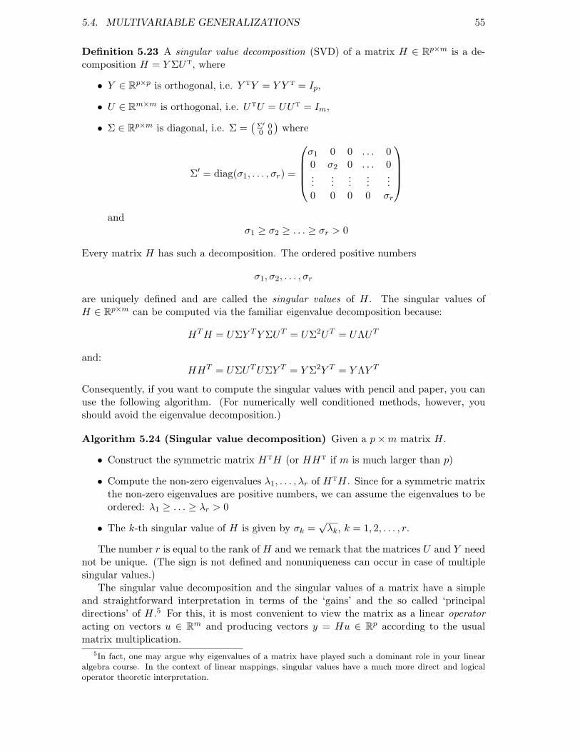
5.4. MULTIVARIABLE GENERALIZATIONS 55
Definition 5.23 A singular value decomposition (SVD) of a matrix H ∈ Rp×m is a de-composition H = Y ΣUT, where
• Y ∈ Rp×p is orthogonal, i.e. Y TY = Y Y T = Ip,
• U ∈ Rm×m is orthogonal, i.e. UTU = UUT = Im,
• Σ ∈ Rp×m is diagonal, i.e. Σ =(
Σ′ 00 0
)where
Σ′ = diag(σ1, . . . , σr) =
σ1 0 0 . . . 00 σ2 0 . . . 0...
......
......
0 0 0 0 σr
and
σ1 ≥ σ2 ≥ . . . ≥ σr > 0
Every matrix H has such a decomposition. The ordered positive numbers
σ1, σ2, . . . , σr
are uniquely defined and are called the singular values of H. The singular values ofH ∈ Rp×m can be computed via the familiar eigenvalue decomposition because:
HTH = UΣY TY ΣUT = UΣ2UT = UΛUT
and:HHT = UΣUTUΣY T = Y Σ2Y T = Y ΛY T
Consequently, if you want to compute the singular values with pencil and paper, you canuse the following algorithm. (For numerically well conditioned methods, however, youshould avoid the eigenvalue decomposition.)
Algorithm 5.24 (Singular value decomposition) Given a p×m matrix H.
• Construct the symmetric matrix HTH (or HHT if m is much larger than p)
• Compute the non-zero eigenvalues λ1, . . . , λr of HTH. Since for a symmetric matrixthe non-zero eigenvalues are positive numbers, we can assume the eigenvalues to beordered: λ1 ≥ . . . ≥ λr > 0
• The k-th singular value of H is given by σk =√λk, k = 1, 2, . . . , r.
The number r is equal to the rank of H and we remark that the matrices U and Y neednot be unique. (The sign is not defined and nonuniqueness can occur in case of multiplesingular values.)
The singular value decomposition and the singular values of a matrix have a simpleand straightforward interpretation in terms of the ‘gains’ and the so called ‘principaldirections’ of H.5 For this, it is most convenient to view the matrix as a linear operatoracting on vectors u ∈ Rm and producing vectors y = Hu ∈ Rp according to the usualmatrix multiplication.
5In fact, one may argue why eigenvalues of a matrix have played such a dominant role in your linearalgebra course. In the context of linear mappings, singular values have a much more direct and logicaloperator theoretic interpretation.
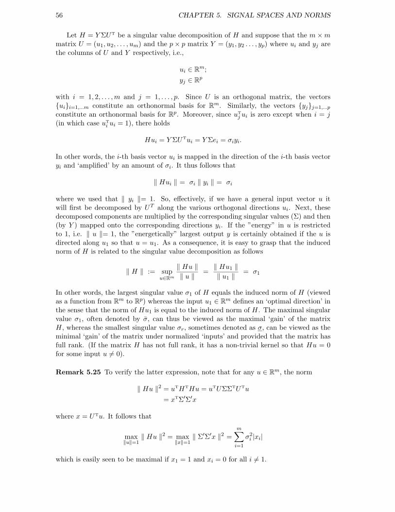
56 CHAPTER 5. SIGNAL SPACES AND NORMS
Let H = Y ΣUT be a singular value decomposition of H and suppose that the m×mmatrix U = (u1, u2, . . . , um) and the p× p matrix Y = (y1, y2 . . . , yp) where ui and yj arethe columns of U and Y respectively, i.e.,
ui ∈ Rm;yj ∈ Rp
with i = 1, 2, . . . ,m and j = 1, . . . , p. Since U is an orthogonal matrix, the vectorsuii=1,...m constitute an orthonormal basis for Rm. Similarly, the vectors yjj=1,...p
constitute an orthonormal basis for Rp. Moreover, since uTj ui is zero except when i = j
(in which case uTi ui = 1), there holds
Hui = Y ΣUTui = Y Σei = σiyi.
In other words, the i-th basis vector ui is mapped in the direction of the i-th basis vectoryi and ‘amplified’ by an amount of σi. It thus follows that
‖ Hui ‖ = σi ‖ yi ‖ = σi
where we used that ‖ yi ‖= 1. So, effectively, if we have a general input vector u itwill first be decomposed by UT along the various orthogonal directions ui. Next, thesedecomposed components are multiplied by the corresponding singular values (Σ) and then(by Y ) mapped onto the corresponding directions yi. If the ”energy” in u is restrictedto 1, i.e. ‖ u ‖= 1, the ”energetically” largest output y is certainly obtained if the u isdirected along u1 so that u = u1. As a consequence, it is easy to grasp that the inducednorm of H is related to the singular value decomposition as follows
‖ H ‖ := supu∈Rm
‖ Hu ‖‖ u ‖ =
‖ Hu1 ‖‖ u1 ‖ = σ1
In other words, the largest singular value σ1 of H equals the induced norm of H (viewedas a function from Rm to Rp) whereas the input u1 ∈ Rm defines an ‘optimal direction’ inthe sense that the norm of Hu1 is equal to the induced norm of H. The maximal singularvalue σ1, often denoted by σ, can thus be viewed as the maximal ‘gain’ of the matrixH, whereas the smallest singular value σr, sometimes denoted as σ, can be viewed as theminimal ‘gain’ of the matrix under normalized ‘inputs’ and provided that the matrix hasfull rank. (If the matrix H has not full rank, it has a non-trivial kernel so that Hu = 0for some input u = 0).
Remark 5.25 To verify the latter expression, note that for any u ∈ Rm, the norm
‖ Hu ‖2 = uTHTHu = uTUΣΣTUTu
= xTΣ′Σ′x
where x = UTu. It follows that
max‖u‖=1
‖ Hu ‖2 = max‖x‖=1
‖ Σ′Σ′x ‖2 =m∑
i=1
σ2i |xi|
which is easily seen to be maximal if x1 = 1 and xi = 0 for all i = 1.

5.4. MULTIVARIABLE GENERALIZATIONS 57
5.4.2 The H∞ norm for multivariable systems
Consider the p×m stable transfer function H(s) and let
H(jω) = Y (jω)Σ(jω)U∗(jω)
be a singular value decomposition of H(jω) for a fixed value of ω ∈ R. Since H(jω) isin general complex valued, we have that H(jω) ∈ Cp×m and the singular vectors storedin Y (jω) and U(jω) are complex valued. For each such ω, the singular values, still beingreal valued (i.e. σi ∈ R), are ordered according to
σ1(ω) ≥ σ2(ω) ≥ . . . ≥ σr(ω) > 0
where r is equal to the rank of H(s) and in general equal to the minimum of p and m.Thus the singular values become frequency dependent! From the previous section we inferthat for each ω ∈ R
0 ≤ ‖ H(jω)u(ω) ‖‖ u(ω) ‖ ≤ σ1(ω)
or, stated otherwise,‖ H(jω)u(ω) ‖ ≤ σ1(ω) ‖ u(ω) ‖
so that σ(ω) := σ1(ω) viewed as a function of ω has the interpretation of a maximal gainof the system at frequency ω. It is for this reason that a plot of σ(ω) with ω ∈ R can beviewed as a multivariable generalization of the Bode diagram!
Definition 5.26 Let H(s) be a stable multivariable transfer function. The H∞ norm ofH(s) is defined as
‖ H(s) ‖∞:= supω∈R
σ(H(jω)).
With this definition we obtain the natural generalization of the results of section 5.3 formultivariable systems. Indeed, we have the following multivariable analog of theorem 5.16:
Theorem 5.27 Let T = R+ or T = R be the time set. For a stable multivariable transferfunction H(s) the L2 induced norm and the power induced norm is equal to the H∞ normof H(s). That is,
‖ H ‖(2,2)=‖ H ‖pow=‖ H(s) ‖∞The derivation of this result is to a large extent similar to the one given in (5.23). An
example of a “multivariable Bode diagram”’ is depicted in Figure 5.4.The bottom line of this subsection is therefore that the L2-induced operator norm and
the power-induced norm of a system is equal to the H∞ norm of its tranfer function.
5.4.3 The H2 norm for multivariable systems
The H2 norm of a p×m transfer function H(s) is defined as follows.
Definition 5.28 Let H(s) be a stable multivariable transfer function of dimension p×m.The H2 norm of H(s) is defined as
‖ H(s) ‖H2=1
2
∫ ∞
−∞trace [H∗(−jω)H(jω)]dω
1/2.
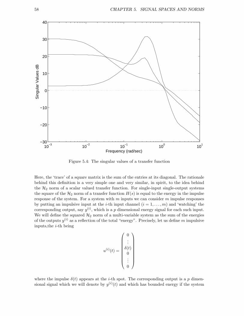
58 CHAPTER 5. SIGNAL SPACES AND NORMS
10−3
10−2
10−1
100
101
−30
−20
−10
0
10
20
30
40
Frequency (rad/sec)
Sin
gula
r V
alue
s dB
Figure 5.4: The singular values of a transfer function
Here, the ‘trace’ of a square matrix is the sum of the entries at its diagonal. The rationalebehind this definition is a very simple one and very similar, in spirit, to the idea behindthe H2 norm of a scalar valued transfer function. For single-input single-output systemsthe square of the H2 norm of a transfer function H(s) is equal to the energy in the impulseresponse of the system. For a system with m inputs we can consider m impulse responsesby putting an impulsive input at the i-th input channel (i = 1, . . . ,m) and ‘watching’ thecorresponding output, say y(i), which is a p dimensional energy signal for each such input.We will define the squared H2 norm of a multi-variable system as the sum of the energiesof the outputs y(i) as a reflection of the total “energy”. Precisely, let us define m impulsiveinputs,the i-th being
u(i)(t) =
0...
δ(t)0...0
where the impulse δ(t) appears at the i-th spot. The corresponding output is a p dimen-sional signal which we will denote by y(i)(t) and which has bounded energy if the system

5.4. MULTIVARIABLE GENERALIZATIONS 59
is assumed to be stable. The square of its two norm is given by
‖ y(i) ‖22 :=∫ ∞
−∞
p∑j=1
|y(i)j (t)|2dt
where y(i)j denotes the j-th component of the output due to an impulsive input at the i-th
input channel.The H2 norm of the transfer function H(s) is nothing else than the square root of the
sum of the two-norms of these outputs. That is:
‖ H(s) ‖2H2=
m∑i=1
‖ y(i) ‖22 .
In a stochastic setting, an m dimensional (stationary) stochastic process admits anm-dimensional mean µ = E [u(t)] which is is independent of t, whereas its second ordermoments E [u(t1)u(t2)T] now define m ×m matrices which only depend on the time dif-ference t1 − t2. As in the previous section, we derive that the infinite horizon RMS valueequals the H2 norm of the system, i.e.,
‖H‖2RMS =∫ ∞
−∞trace[h(t)hT(t)] dt = ‖H‖2H2
.
60 CHAPTER 5. SIGNAL SPACES AND NORMS
5.5 Exercises
1. Consider the following continuous time signals and determine their amplitude (‖· ‖∞), their energy (‖ · ‖2) and their L1 norm (‖ · ‖1).
(a) x(t) =
0 for t < 01
1+t for t ≥ 0
(b) x(t) = cos(2πft) for fixed real frequency f > 0.
(c) x(t) = exp(α|t|) for fixed α. Distinguish the cases where α > 0, α < 0 andα = 0.
2. This exercise is mainly meant to familiarize you with various routines and proceduresin MATLAB. This exercise involves a single input single output control scheme andshould be viewed as a ‘prelude’ for the multivariable control scheme of an exercisebelow.
Consider a single input single output system described by the transfer function
P (s) =−s
(s+ 1)(s+ 2).
The system P is controlled by the constant controller C(s) = 1. We consider theusual feedback interconnection of P and C as described earlier.
(a) Determine the H∞ norm of the system P .Hint: You can represent the plant P in MATLAB by introducing the numerator(‘teller’) and the denominator (‘noemer’) polynomial coefficients separately. Since(s + 1)(s + 2) = s2 + 3s + 2 the denominator polynomial is represented by a vari-able den=[1 3 2] (coefficients always in descending order). Similarly, the numeratorpolynomial of P is represented by num=[0 -1 0]. The H∞ norm of P can now beread from the Bode plot of P by invoking the procedure bode(num,den).
(b) Determine the H∞ norm of the sensitivity S, the complementary sensitivity Tand the control sensitivity R of the closed loop system.Hint: The feedback interconnection of P and C can be obtained by the MATLAB pro-cedures feedbk or feedback. After reading the help information about this procedure(help feedbk) we learn that the procedure requires state space representations of Pand C and produces a state space representation of the closed loop system. Make surethat you use the right ‘type’ option to obtain S, T and R, respectively. A state spacerepresentation of P can be obtained, e.g., by invoking the routine tf2ss (‘transfer-to-state-space’). Thus, [a,b,c,d]= tf2ss(num,den) gives a state space description of P .If you prefer a transfer function description of the closed loop to determine the H∞norms, then try the conversion routine ss2tf. See the corresponding help information.
Chapter 6
Weighting filters
6.1 The use of weighting filters
6.1.1 Introduction
The H∞ norm of an input-output system has been shown to be equal to
‖ H(s) ‖∞ = supω∈R
σ(H(jω)) = supu∈L2
‖ H(u) ‖2‖ u ‖2
The H∞ norm therefore indicates the maximal gain of the system if the inputs are al-lowed to vary over the class of signals with bounded two-norm. The frequency dependentmaximal singular value σ(ω), viewed as a function of ω, provides obviously more detailedinformation about the gain characteristics of the system than the H∞ norm only.
For example, if a system is known to be all pass, meaning that the two-norm of theoutput is equal to the two-norm of the input for all possible inputs u, then at everyfrequency ω the maximal gain σ(H(jω)) of the system is constant and equal to the H∞norm ‖ H(s) ‖∞. The system is then said to have a flat spectrum. This in contrast tolow-pass or high-pass systems in which the function σ(ω) vanishes(or is attenuated) athigh frequencies and low frequencies, respectively.
It is this function, σ(jω), that is extensively manipulated in H∞ control system designto meet desired performance objectives. These manipulations are carried out by choosingappropriate weights on the signals entering and leaving a control configuration like forexample the one of Figure 6.1. The specification of these weights is of crucial importancefor the overall control design and is one of the few aspects inH∞ robust control design thatcan not be automated. The choice of appropriate weighting filters is a typical ‘engineeringskill’ which is based on a few simple mathematical observations, and a good insight in theperformance specifications one wishes to achieve.
6.1.2 Singular value loop shaping
Consider the multivariable feedback control system of Figure 6.1 As mentioned before,the multivariable stability margins and performance specifications can be quantified byconsidering the frequency dependent singular values of the various closed-loop systemswhich we can distinguish in Figure 6.1
In this configuration we distinguish various ‘closed-loop’ transfer functions:
• The sensitivityS = (I + PC)−1
61
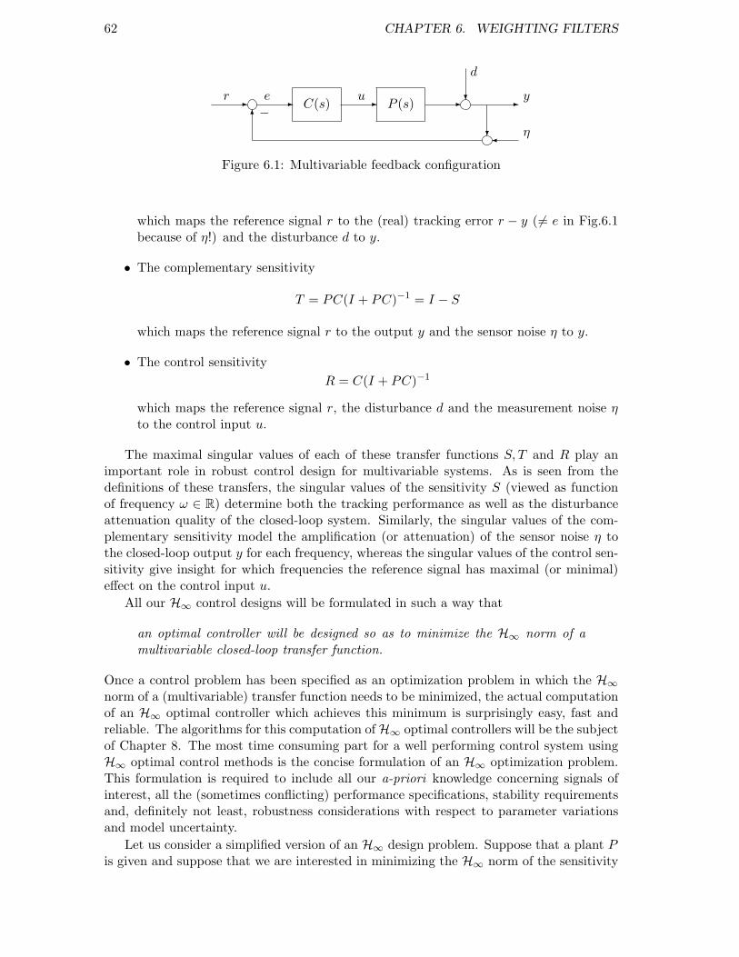
62 CHAPTER 6. WEIGHTING FILTERS
r
e
− C(s) u P (s)
d
y
η
Figure 6.1: Multivariable feedback configuration
which maps the reference signal r to the (real) tracking error r − y (= e in Fig.6.1because of η!) and the disturbance d to y.
• The complementary sensitivity
T = PC(I + PC)−1 = I − S
which maps the reference signal r to the output y and the sensor noise η to y.
• The control sensitivityR = C(I + PC)−1
which maps the reference signal r, the disturbance d and the measurement noise ηto the control input u.
The maximal singular values of each of these transfer functions S, T and R play animportant role in robust control design for multivariable systems. As is seen from thedefinitions of these transfers, the singular values of the sensitivity S (viewed as functionof frequency ω ∈ R) determine both the tracking performance as well as the disturbanceattenuation quality of the closed-loop system. Similarly, the singular values of the com-plementary sensitivity model the amplification (or attenuation) of the sensor noise η tothe closed-loop output y for each frequency, whereas the singular values of the control sen-sitivity give insight for which frequencies the reference signal has maximal (or minimal)effect on the control input u.
All our H∞ control designs will be formulated in such a way that
an optimal controller will be designed so as to minimize the H∞ norm of amultivariable closed-loop transfer function.
Once a control problem has been specified as an optimization problem in which the H∞norm of a (multivariable) transfer function needs to be minimized, the actual computationof an H∞ optimal controller which achieves this minimum is surprisingly easy, fast andreliable. The algorithms for this computation ofH∞ optimal controllers will be the subjectof Chapter 8. The most time consuming part for a well performing control system usingH∞ optimal control methods is the concise formulation of an H∞ optimization problem.This formulation is required to include all our a-priori knowledge concerning signals ofinterest, all the (sometimes conflicting) performance specifications, stability requirementsand, definitely not least, robustness considerations with respect to parameter variationsand model uncertainty.
Let us consider a simplified version of an H∞ design problem. Suppose that a plant Pis given and suppose that we are interested in minimizing the H∞ norm of the sensitivity
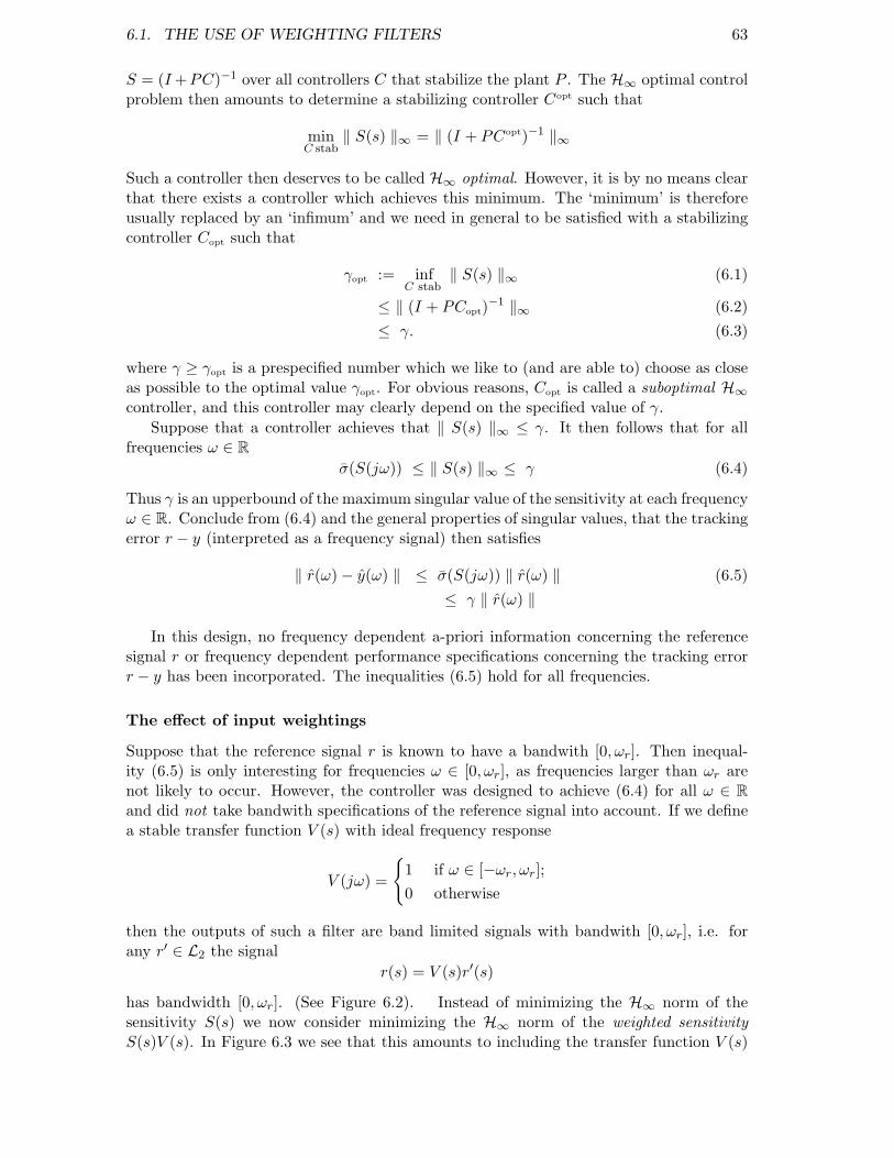
6.1. THE USE OF WEIGHTING FILTERS 63
S = (I+PC)−1 over all controllers C that stabilize the plant P . The H∞ optimal controlproblem then amounts to determine a stabilizing controller Copt such that
minC stab
‖ S(s) ‖∞ = ‖ (I + PCopt)−1 ‖∞
Such a controller then deserves to be called H∞ optimal. However, it is by no means clearthat there exists a controller which achieves this minimum. The ‘minimum’ is thereforeusually replaced by an ‘infimum’ and we need in general to be satisfied with a stabilizingcontroller Copt such that
γopt := infC stab
‖ S(s) ‖∞ (6.1)
≤ ‖ (I + PCopt)−1 ‖∞ (6.2)≤ γ. (6.3)
where γ ≥ γopt is a prespecified number which we like to (and are able to) choose as closeas possible to the optimal value γopt. For obvious reasons, Copt is called a suboptimal H∞controller, and this controller may clearly depend on the specified value of γ.
Suppose that a controller achieves that ‖ S(s) ‖∞ ≤ γ. It then follows that for allfrequencies ω ∈ R
σ(S(jω)) ≤ ‖ S(s) ‖∞ ≤ γ (6.4)
Thus γ is an upperbound of the maximum singular value of the sensitivity at each frequencyω ∈ R. Conclude from (6.4) and the general properties of singular values, that the trackingerror r − y (interpreted as a frequency signal) then satisfies
‖ r(ω)− y(ω) ‖ ≤ σ(S(jω)) ‖ r(ω) ‖ (6.5)≤ γ ‖ r(ω) ‖
In this design, no frequency dependent a-priori information concerning the referencesignal r or frequency dependent performance specifications concerning the tracking errorr − y has been incorporated. The inequalities (6.5) hold for all frequencies.
The effect of input weightings
Suppose that the reference signal r is known to have a bandwith [0, ωr]. Then inequal-ity (6.5) is only interesting for frequencies ω ∈ [0, ωr], as frequencies larger than ωr arenot likely to occur. However, the controller was designed to achieve (6.4) for all ω ∈ R
and did not take bandwith specifications of the reference signal into account. If we definea stable transfer function V (s) with ideal frequency response
V (jω) =
1 if ω ∈ [−ωr, ωr];0 otherwise
then the outputs of such a filter are band limited signals with bandwith [0, ωr], i.e. forany r′ ∈ L2 the signal
r(s) = V (s)r′(s)
has bandwidth [0, ωr]. (See Figure 6.2). Instead of minimizing the H∞ norm of thesensitivity S(s) we now consider minimizing the H∞ norm of the weighted sensitivityS(s)V (s). In Figure 6.3 we see that this amounts to including the transfer function V (s)
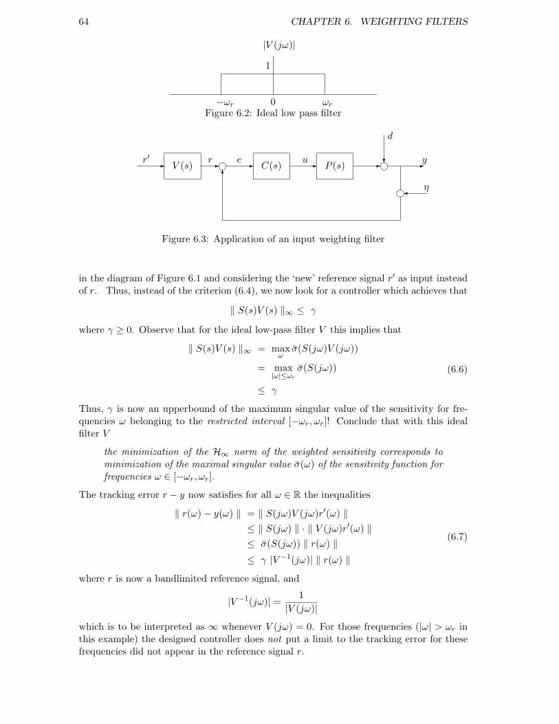
64 CHAPTER 6. WEIGHTING FILTERS
|V (jω)|1
0−ωr ωr
Figure 6.2: Ideal low pass filter
V (s)r′r
e C(s) u P (s)
d
y
η
Figure 6.3: Application of an input weighting filter
in the diagram of Figure 6.1 and considering the ‘new’ reference signal r′ as input insteadof r. Thus, instead of the criterion (6.4), we now look for a controller which achieves that
‖ S(s)V (s) ‖∞ ≤ γ
where γ ≥ 0. Observe that for the ideal low-pass filter V this implies that
‖ S(s)V (s) ‖∞ = maxω
σ(S(jω)V (jω))
= max|ω|≤ωr
σ(S(jω))
≤ γ
(6.6)
Thus, γ is now an upperbound of the maximum singular value of the sensitivity for fre-quencies ω belonging to the restricted interval [−ωr, ωr]! Conclude that with this idealfilter V
the minimization of the H∞ norm of the weighted sensitivity corresponds tominimization of the maximal singular value σ(ω) of the sensitivity function forfrequencies ω ∈ [−ωr, ωr].
The tracking error r − y now satisfies for all ω ∈ R the inequalities
‖ r(ω)− y(ω) ‖ = ‖ S(jω)V (jω)r′(ω) ‖≤ ‖ S(jω) ‖ · ‖ V (jω)r′(ω) ‖≤ σ(S(jω)) ‖ r(ω) ‖≤ γ |V −1(jω)| ‖ r(ω) ‖
(6.7)
where r is now a bandlimited reference signal, and
|V −1(jω)| = 1|V (jω)|
which is to be interpreted as ∞ whenever V (jω) = 0. For those frequencies (|ω| > ωr inthis example) the designed controller does not put a limit to the tracking error for thesefrequencies did not appear in the reference signal r.
6.1. THE USE OF WEIGHTING FILTERS 65
The last inequality in (6.7) is the most useful one and it follows from the more generalobservation that, whenever ‖ S(s)V (s) ‖∞≤ γ with V a square stable transfer functionwhose inverse V −1 is again stable, then for all ω ∈ R there holds
σ[S(jω)] = σ[S(jω)V (jω)V −1(jω)]
≤ σ[S(jω)V (jω)]σ[V −1(jω)]
≤ γσ[V −1(jω)]
We thus come to the important conclusion that
a controller C which achieves that the weighted sensitivity
‖ S(s)V (s) ‖∞ ≤ γ
results in a closed loop system in which
σ(S(jω)) ≤ γσ[V −1(jω)] (6.8)
Remark 6.1 This conclusion holds for any stable weighting filter V (s) whose inverseV −1(s) is again a stable transfer function. This is questionable for the ideal filter V weused here to illustrate the effect, because for ω > ωr the inverse filter V (jω)−1 can bequalified as unstable. In practice we will therefore choose filters which have a rationaltransfer function being stable, minimum phase and biproper. An alternative first orderfilter for this example could thus have been e.g. V (s) = (s+100ωr)
100(s+ωr) .
Remark 6.2 It is a standard property of the singular value decomposition that,wheneverV −1(jω) exists,
σ[V −1(jω)] =1
σ[V (jω)]
where σ denotes the smallest singular value.
The effect of output weightings
In the previous subsection we considered the effect of applying a weighting filter for aninput signal. Likewise, we can also define weighting filters on the output signals whichoccur in a closed-loop configuration as in Figure 6.1.
We consider again (as an example) the sensitivity S(s) viewed as a mapping fromthe reference input r to the tracking error r − y = e, when we fully disregard for themoment the measurement noise η. A straightforward H∞ design would minimize the H∞norm of the sensitivity S(s) and result in the upperbound (6.5) for the tracking error.We could, however, be interested in minimizing the spectrum of the tracking error atspecific frequencies only. Let us suppose that we are interested in the tracking error e atfrequencies ω ≤ ω ≤ ω only, where ω > 0 and ω > 0 define a lower and upperbound. Asin the previous subsection, we introduce a new signal
e′(s) = W (s)e(s)
where W is a (stable) transfer function whose frequency response is ideally defined by theband pass filter
W (jω) =
1 if ω ≤ |ω| ≤ ω;0 otherwise
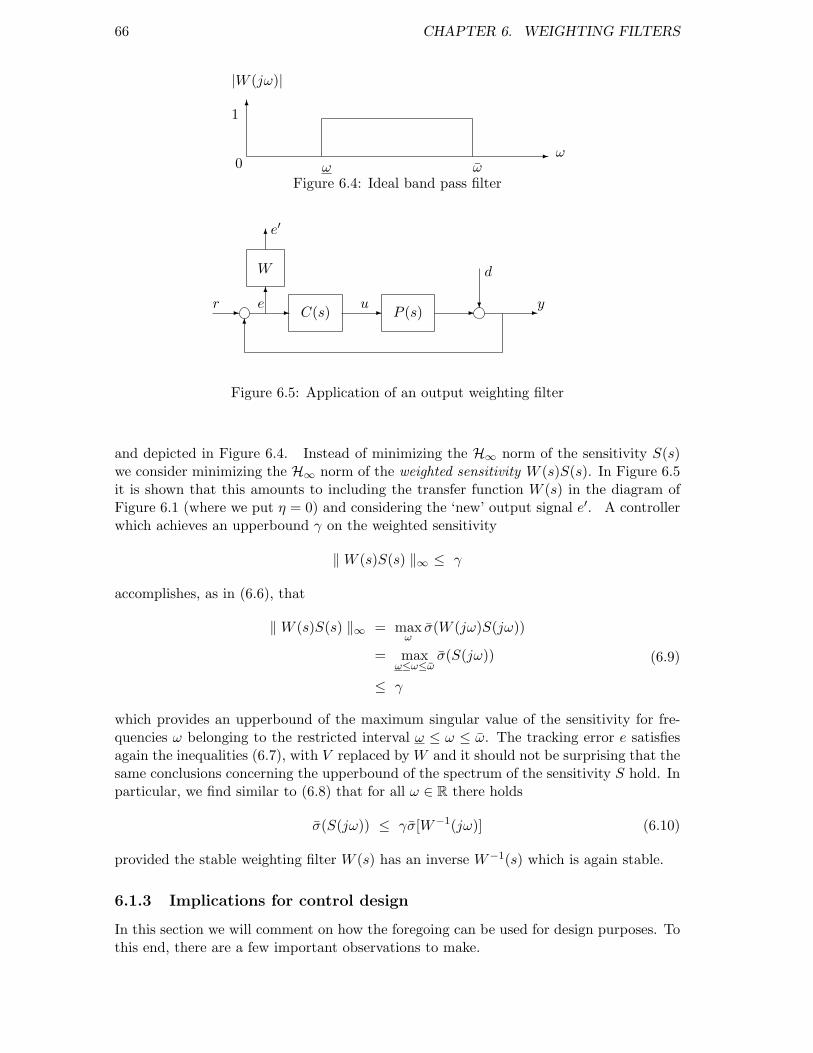
66 CHAPTER 6. WEIGHTING FILTERS
|W (jω)|
ω0 ω ω
1
Figure 6.4: Ideal band pass filter
r
e
W
e′
C(s) u P (s)
d
y
Figure 6.5: Application of an output weighting filter
and depicted in Figure 6.4. Instead of minimizing the H∞ norm of the sensitivity S(s)we consider minimizing the H∞ norm of the weighted sensitivity W (s)S(s). In Figure 6.5it is shown that this amounts to including the transfer function W (s) in the diagram ofFigure 6.1 (where we put η = 0) and considering the ‘new’ output signal e′. A controllerwhich achieves an upperbound γ on the weighted sensitivity
‖W (s)S(s) ‖∞ ≤ γ
accomplishes, as in (6.6), that
‖W (s)S(s) ‖∞ = maxω
σ(W (jω)S(jω))
= maxω≤ω≤ω
σ(S(jω))
≤ γ
(6.9)
which provides an upperbound of the maximum singular value of the sensitivity for fre-quencies ω belonging to the restricted interval ω ≤ ω ≤ ω. The tracking error e satisfiesagain the inequalities (6.7), with V replaced by W and it should not be surprising that thesame conclusions concerning the upperbound of the spectrum of the sensitivity S hold. Inparticular, we find similar to (6.8) that for all ω ∈ R there holds
σ(S(jω)) ≤ γσ[W−1(jω)] (6.10)
provided the stable weighting filter W (s) has an inverse W−1(s) which is again stable.
6.1.3 Implications for control design
In this section we will comment on how the foregoing can be used for design purposes. Tothis end, there are a few important observations to make.
6.1. THE USE OF WEIGHTING FILTERS 67
• For one thing, we showed in subsection 6.1.2 that by choosing the frequency responseof an input weighting filter V (s) so as to ‘model’ the frequency characteristic of theinput signal r, the a-priori information of this reference signal has been incorporatedin the controller design. By doing so, the minimization of the maximum singularvalue of the sensitivity S(s) has been refined (like in (6.6)) to the frequency intervalof interest. Clearly, we can do this for any input signal.
• Secondly, we obtained in (6.8) and in (6.10) frequency dependent upperbounds forthe maximum gain of the sensitivity. Choosing V (jω) (or W (jω)) appropriately,enables one to specify the frequency attenuation of the closed-loop transfer function(the sensitivity in this case). Indeed, choosing, for example, V (jω) a low pass transferfunction implies that V −1(jω) is a high pass upper-bound on the frequency spectrumof the closed-loop transfer function. Using (6.8) this implies that low frequencies ofthe sensitivity are attenuated and that the frequency characteristic of V has ‘shaped’the frequency characteristic of S. The same kind of ‘loop-shaping’ can be achievedby either choosing input or output weightings.
• Thirdly, by applying weighting factors to both input signals and output signalswe can minimize (for example) the H∞ norm of the two-sided weighted sensitivityW (s)S(s)V (s), i.e., a controller could be designed so as to achieve that
‖W (s)S(s)V (s) ‖∞ ≤ γ
for some γ > 0. Provided the transfer functions V (s) and W (s) have stable inverses,this leads to a frequency dependent upperbound for the original sensitivity. Precisely,in this case
σ(S(jω)) ≤ γσ[V −1(jω)]σ[W−1(jω)] (6.11)
from which we see that the frequency characteristic of the sensitivity is shapedby both V as well as W . It is precisely this formula that provides you with awealth of design possibilities! Once a performance requirement for a closed-looptransfer function (let’s say the sensitivity S(s)) is specified in terms of its frequencycharacteristic, this characteristic needs to be ‘modeled’ by the frequency responseof the product V −1(jω)W−1(jω) by choosing the input and output filters V andW appropriately. A controller C(s) that bounds the H∞ norm of the weightedsensitivity W (s)S(s)V (s) then achieves the desired characteristic by equation (6.11).
The weighting filters V and W on input and output signals of a closed-loop transferfunction give therefore the possibility to shape the spectrum of that specific closed-looptransfer. Once these filters are specified, a controller is computed to minimize the H∞norm of the weighted transfer and results in a closed-loop transfer whose spectrum hasbeen shaped according to (6.11).
In the example of a weighted sensitivity, the controller C is thus computed to establishthat
γfilt := infC stab
‖W (s)S(s)V (s) ‖∞ (6.12)
≤ ‖W (s)(I + PC)−1V (s) ‖∞ (6.13)≤ γ. (6.14)
for some γ > 0 which is as close as possible to γfilt (which depends on the plant P andthe choice of the weigthing filters V and W ). To find such a γ larger than or equal to the
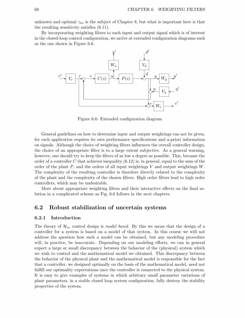
68 CHAPTER 6. WEIGHTING FILTERS
unknown and optimal γfilt is the subject of Chapter 8, but what is important here is thatthe resulting sensitivity satisfies (6.11).
By incorporating weighting filters to each input and output signal which is of interestin the closed-loop control configuration, we arrive at extended configuration diagrams suchas the one shown in Figure 6.6.
r′
Vrr
e We e′
v C(s) u
Wu
u′
P (s) d
Vd
d′
y Wy y′
Vη η′η
Figure 6.6: Extended configuration diagram
General guidelines on how to determine input and output weightings can not be given,for each application requires its own performance specifications and a-priori informationon signals. Although the choice of weighting filters influences the overall controller design,the choice of an appropriate filter is to a large extent subjective. As a general warning,however, one should try to keep the filters of as low a degree as possible. This, because theorder of a controller C that achieves inequality (6.12) is, in general, equal to the sum of theorder of the plant P , and the orders of all input weightings V and output weightings W .The complexity of the resulting controller is therefore directly related to the complexityof the plant and the complexity of the chosen filters. High order filters lead to high ordercontrollers, which may be undesirable.
More about appropriate weighting filters and their interactive effects on the final so-lution in a complicated scheme as Fig. 6.6 follows in the next chapters.
6.2 Robust stabilization of uncertain systems
6.2.1 Introduction
The theory of H∞ control design is model based. By this we mean that the design of acontroller for a system is based on a model of that system. In this course we will notaddress the question how such a model can be obtained, but any modeling procedurewill, in practice, be inaccurate. Depending on our modeling efforts, we can in generalexpect a large or small discrepancy between the behavior of the (physical) system whichwe wish to control and the mathematical model we obtained. This discrepancy betweenthe behavior of the physical plant and the mathematical model is responsible for the factthat a controller, we designed optimally on the basis of the mathematical model, need notfulfill our optimality expectations once the controller is connected to the physical system.It is easy to give examples of systems in which arbitrary small parameter variations ofplant parameters, in a stable closed loop system configuration, fully destroy the stabilityproperties of the system.

6.2. ROBUST STABILIZATION OF UNCERTAIN SYSTEMS 69
Robust stability refers to the ability of a closed loop stable system to remain stable inthe presence of modeling errors. For this, one needs to have some insight in the accuracyof a mathematical model which represents the physical system we wish to control. Thereare many ways to do this:
• One can take a stochastic approach and attach a certain likelihood or probabilityto the elements of a class of models which are assumed to represent the unknown,(often called ‘true’) system.
• One can define a class of models each of which is equally acceptable to model theunknown physical system
• One can select one nominal model together with a description of its uncertainty interms of its parameters, in terms of its frequency response, in terms of its impulseresponse, etc. In this case, the uncertain part of a process is modeled separatelyfrom the known (nominal) part.
For each of these possibilities a quantification of model uncertainty is necessary and es-sential for the design of controllers which are robust against those uncertainties.
In practice, the design of controllers is often based on various iterations of the loop
data collection −→ modeling −→ controller design −→ validation
in which improvement of performance of the previous iteration is the main aim.In this chapter we analyze robust stability of a control system. We introduce various
ways to represent model uncertainty and we will study to what extent these uncertaintydescriptions can be taken into account to design robustly stabilizing controllers.
6.2.2 Modeling model errors
It may sound somewhat paradoxial to model dynamics of a system which one deliberatelydecided not to take into account in the modeling phase. Our purpose here will be to onlyprovide upperbounds on modeling errors. Various approaches are possible
• model errors can be quantified in the time domain. Typical examples include de-scriptions of variations in the physical parameters in a state space model.
• alternatively, model errors can be quantified in the frequency domain by analyzingperturbations of transfer functions or frequency responses.
We will basically concentrate on the latter in this chapter. For frequency domain modeluncertainty descriptions one usually distinguishes two approaches, which lead to differentresearch directions:
• Unstructured uncertainty: model uncertainty is expressed only in terms of upper-bounds on errors of frequency responses. No more information on the origin of themodeling errors is used.
• Structured uncertainty: apart from an upperbound on the modeling errors, also thespecific structure in uncertainty of parameters is taken into account.
For the analysis of unstructured model uncertainty in the frequency domain there arefour main uncertainty models which we briefly review.
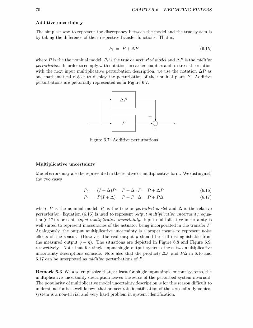
70 CHAPTER 6. WEIGHTING FILTERS
Additive uncertainty
The simplest way to represent the discrepancy between the model and the true system isby taking the difference of their respective transfer functions. That is,
Pt = P + ∆P (6.15)
where P is the the nominal model, Pt is the true or perturbed model and ∆P is the additiveperturbation. In order to comply with notations in earlier chapters and to stress the relationwith the next input multiplicative perturbation description, we use the notation ∆P asone mathematical object to display the perturbation of the nominal plant P . Additiveperturbations are pictorially represented as in Figure 6.7.
P +
∆P
+
Figure 6.7: Additive perturbations
Multiplicative uncertainty
Model errors may also be represented in the relative or multiplicative form. We distinguishthe two cases
Pt = (I + ∆)P = P + ∆ · P = P + ∆P (6.16)Pt = P (I + ∆) = P + P ·∆ = P + P∆ (6.17)
where P is the nominal model, Pt is the true or perturbed model and ∆ is the relativeperturbation. Equation (6.16) is used to represent output multiplicative uncertainty, equa-tion(6.17) represents input multiplicative uncertainty. Input multiplicative uncertainty iswell suited to represent inaccuracies of the actuator being incorporated in the transfer P .Analogously, the output multiplicative uncertainty is a proper means to represent noiseeffects of the sensor. (However, the real output y should be still distinguishable fromthe measured output y + η). The situations are depicted in Figure 6.8 and Figure 6.9,respectively. Note that for single input single output systems these two multiplicativeuncertainty descriptions coincide. Note also that the products ∆P and P∆ in 6.16 and6.17 can be interpreted as additive perturbations of P .
Remark 6.3 We also emphasize that, at least for single input single output systems, themultiplicative uncertainty description leaves the zeros of the perturbed system invariant.The popularity of multiplicative model uncertainty description is for this reason difficult tounderstand for it is well known that an accurate identification of the zeros of a dynamicalsystem is a non-trivial and very hard problem in system identification.
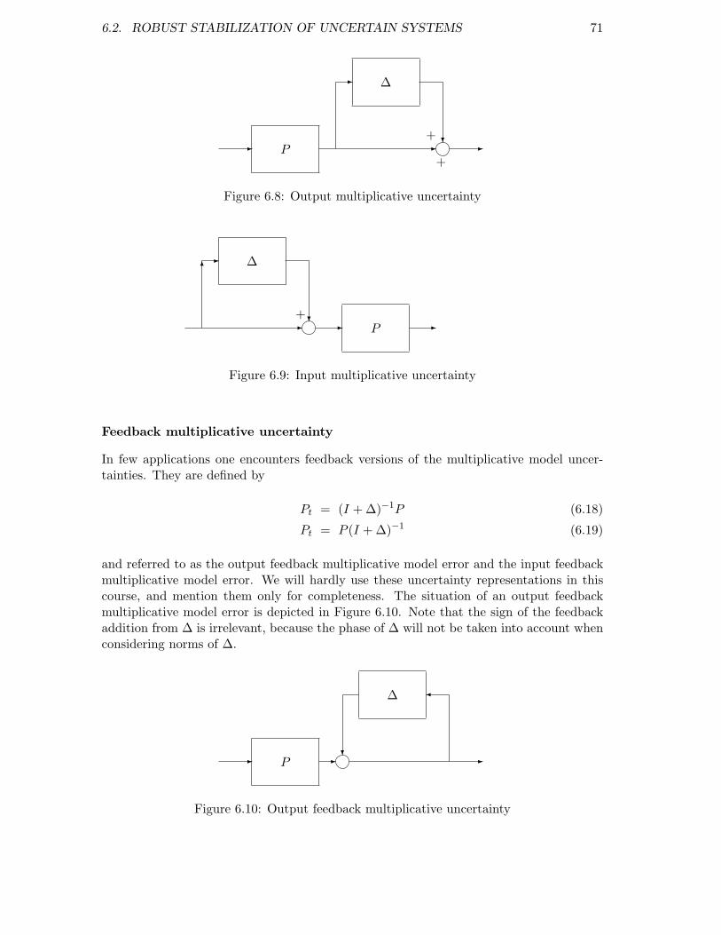
6.2. ROBUST STABILIZATION OF UNCERTAIN SYSTEMS 71
P +
∆
+
Figure 6.8: Output multiplicative uncertainty
+
∆
P
Figure 6.9: Input multiplicative uncertainty
Feedback multiplicative uncertainty
In few applications one encounters feedback versions of the multiplicative model uncer-tainties. They are defined by
Pt = (I + ∆)−1P (6.18)
Pt = P (I + ∆)−1 (6.19)
and referred to as the output feedback multiplicative model error and the input feedbackmultiplicative model error. We will hardly use these uncertainty representations in thiscourse, and mention them only for completeness. The situation of an output feedbackmultiplicative model error is depicted in Figure 6.10. Note that the sign of the feedbackaddition from ∆ is irrelevant, because the phase of ∆ will not be taken into account whenconsidering norms of ∆.
P
∆
Figure 6.10: Output feedback multiplicative uncertainty
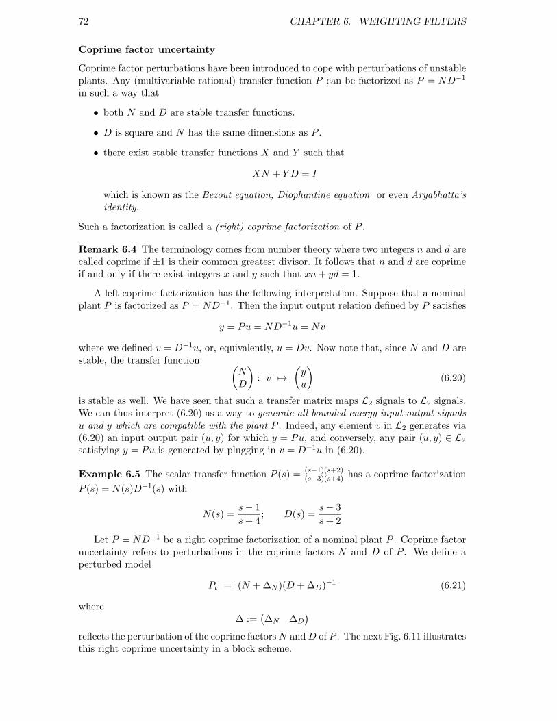
72 CHAPTER 6. WEIGHTING FILTERS
Coprime factor uncertainty
Coprime factor perturbations have been introduced to cope with perturbations of unstableplants. Any (multivariable rational) transfer function P can be factorized as P = ND−1
in such a way that
• both N and D are stable transfer functions.
• D is square and N has the same dimensions as P .
• there exist stable transfer functions X and Y such that
XN + Y D = I
which is known as the Bezout equation, Diophantine equation or even Aryabhatta’sidentity.
Such a factorization is called a (right) coprime factorization of P .
Remark 6.4 The terminology comes from number theory where two integers n and d arecalled coprime if ±1 is their common greatest divisor. It follows that n and d are coprimeif and only if there exist integers x and y such that xn+ yd = 1.
A left coprime factorization has the following interpretation. Suppose that a nominalplant P is factorized as P = ND−1. Then the input output relation defined by P satisfies
y = Pu = ND−1u = Nv
where we defined v = D−1u, or, equivalently, u = Dv. Now note that, since N and D arestable, the transfer function (
ND
): v →
(yu
)(6.20)
is stable as well. We have seen that such a transfer matrix maps L2 signals to L2 signals.We can thus interpret (6.20) as a way to generate all bounded energy input-output signalsu and y which are compatible with the plant P . Indeed, any element v in L2 generates via(6.20) an input output pair (u, y) for which y = Pu, and conversely, any pair (u, y) ∈ L2satisfying y = Pu is generated by plugging in v = D−1u in (6.20).
Example 6.5 The scalar transfer function P (s) = (s−1)(s+2)(s−3)(s+4) has a coprime factorization
P (s) = N(s)D−1(s) with
N(s) =s− 1s+ 4
; D(s) =s− 3s+ 2
Let P = ND−1 be a right coprime factorization of a nominal plant P . Coprime factoruncertainty refers to perturbations in the coprime factors N and D of P . We define aperturbed model
Pt = (N + ∆N )(D + ∆D)−1 (6.21)
where∆ :=
(∆N ∆D
)reflects the perturbation of the coprime factorsN andD of P . The next Fig. 6.11 illustratesthis right coprime uncertainty in a block scheme.
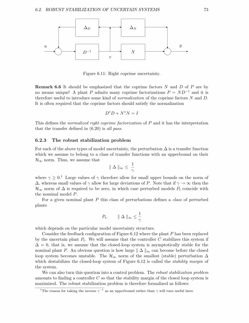
6.2. ROBUST STABILIZATION OF UNCERTAIN SYSTEMS 73
D−1 N
∆D ∆N
u y
v
Figure 6.11: Right coprime uncertainty.
Remark 6.6 It should be emphasized that the coprime factors N and D of P are byno means unique! A plant P admits many coprime factorizations P = ND−1 and it istherefore useful to introduce some kind of normalization of the coprime factors N and D.It is often required that the coprime factors should satisfy the normalization
D∗D +N∗N = I
This defines the normalized right coprime factorization of P and it has the interpretationthat the transfer defined in (6.20) is all pass.
6.2.3 The robust stabilization problem
For each of the above types of model uncertainty, the perturbation ∆ is a transfer functionwhich we assume to belong to a class of transfer functions with an upperbound on theirH∞ norm. Thus, we assume that
‖ ∆ ‖∞ ≤ 1γ
where γ ≥ 0.1 Large values of γ therefore allow for small upper bounds on the norm of∆, whereas small values of γ allow for large deviations of P . Note that if γ →∞ then theH∞ norm of ∆ is required to be zero, in which case perturbed models Pt coincide withthe nominal model P .
For a given nominal plant P this class of perturbations defines a class of perturbedplants
Pt, ‖ ∆ ‖∞ ≤ 1γ
which depends on the particular model uncertainty structure.Consider the feedback configuration of Figure 6.12 where the plant P has been replaced
by the uncertain plant Pt. We will assume that the controller C stabilizes this system if∆ = 0, that is, we assume that the closed-loop system is asymptotically stable for thenominal plant P . An obvious question is how large ‖ ∆ ‖∞ can become before the closedloop system becomes unstable. The H∞ norm of the smallest (stable) perturbation ∆which destabilizes the closed-loop system of Figure 6.12 is called the stability margin ofthe system.
We can also turn this question into a control problem. The robust stabilization problemamounts to finding a controller C so that the stability margin of the closed loop system ismaximized. The robust stabilization problem is therefore formalized as follows:
1The reason for taking the inverse γ−1 as an upperbound rather than γ will turn useful later.
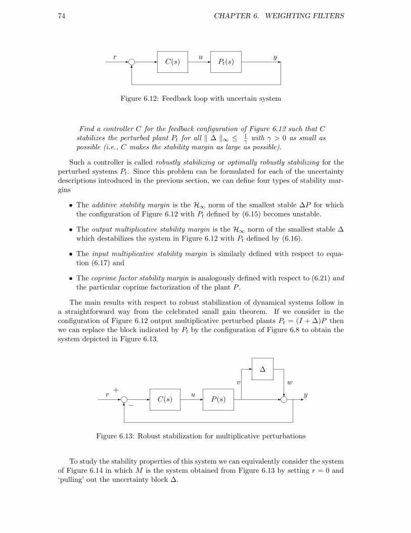
74 CHAPTER 6. WEIGHTING FILTERS
r
C(s) u Pt(s) y
Figure 6.12: Feedback loop with uncertain system
Find a controller C for the feedback configuration of Figure 6.12 such that Cstabilizes the perturbed plant Pt for all ‖ ∆ ‖∞ ≤ 1
γ with γ > 0 as small aspossible (i.e., C makes the stability margin as large as possible).
Such a controller is called robustly stabilizing or optimally robustly stabilizing for theperturbed systems Pt. Since this problem can be formulated for each of the uncertaintydescriptions introduced in the previous section, we can define four types of stability mar-gins
• The additive stability margin is the H∞ norm of the smallest stable ∆P for whichthe configuration of Figure 6.12 with Pt defined by (6.15) becomes unstable.
• The output multiplicative stability margin is the H∞ norm of the smallest stable ∆which destabilizes the system in Figure 6.12 with Pt defined by (6.16).
• The input multiplicative stability margin is similarly defined with respect to equa-tion (6.17) and
• The coprime factor stability margin is analogously defined with respect to (6.21) andthe particular coprime factorization of the plant P .
The main results with respect to robust stabilization of dynamical systems follow ina straightforward way from the celebrated small gain theorem. If we consider in theconfiguration of Figure 6.12 output multiplicative perturbed plants Pt = (I + ∆)P thenwe can replace the block indicated by Pt by the configuration of Figure 6.8 to obtain thesystem depicted in Figure 6.13.
r+
− C(s) u P (s)
v w
∆
y
Figure 6.13: Robust stabilization for multiplicative perturbations
To study the stability properties of this system we can equivalently consider the systemof Figure 6.14 in which M is the system obtained from Figure 6.13 by setting r = 0 and‘pulling’ out the uncertainty block ∆.

6.2. ROBUST STABILIZATION OF UNCERTAIN SYSTEMS 75
M
∆
Figure 6.14: Small gain configuration
For the case of output multiplicative perturbations M maps the signal w to v and thecorresponding transfer function is easily seen to be
M = T = PC(I + PC)−1
i.e., M is precisely the complementary sensitivity transfer function2. Since we assumedthat the controller C stabilizes the nominal plant P it follows that M is a stable transferfunction, independent of the perturbation ∆ but dependent on the choice of the controllerC.
The stability properties of the configuration of Figure 6.13 are determined by the smallgain theorem (Zames, 1966):
Theorem 6.7 (Small gain theorem) Suppose that the systems M and ∆ are both sta-ble. Then the autonomous system determined by the feedback interconnection of Fig-ure 6.14 is asymptotically stable if
‖M∆ ‖∞< 1
For a given controller C the small gain theorem therefore guarantees the stability ofthe closed loop system of Figure 6.14 (and thus also the system of Figure 6.13) provided∆ is stable and satisfies for all ω ∈ R
σ(M(jω)∆(jω)) < 1.
For SISO systems this translates in a condition on the absolute values of the frequencyresponses of M and ∆. Precisely, for all ω ∈ R we should have that
σ(M∆) = |M∆| = |M ||∆| = σ(M)σ(∆)
(where we omitted the argument jω in each transfer) to guarantee the stability of the closedloop system. For MIMO systems we obtain, by using the singular value decomposition,that for all ω ∈ R
σ(M∆) = σ(YMΣMU∗MY∆Σ∆U
∗∆) ≤ σ(M)σ(∆)
(where again every transfer is supposed to be evaluated at jω) and the maximum isreached for Y∆ = UM that can always be accomplished without affecting the constraint‖ ∆ ‖∞< 1
γ . Hence, to obtain robust stability we have to guarantee for both SISO andMIMO systems that
σ[M(jω)]σ[∆(jω)] < 12Like in chapter 3 actually M = −T , but the sign is irrelevant as it can be incorporated in ∆.

76 CHAPTER 6. WEIGHTING FILTERS
for all ω ∈ R. Stated otherwise
σ[∆(jω)] <1
σ[M(jω)]. (6.22)
for all ω ∈ R.
6.2.4 Robust stabilization: main results
Robust stabilization under additive perturbations
Carrying out the above analysis for the case of additive perturbations leads to the followingmain result on robust stabilization in the presence of additive uncertainty.
Theorem 6.8 (Robust stabilization with additive uncertainty) A controller C sta-bilizes Pt = P + ∆P for all ‖ ∆P ‖∞< 1
γ if and only if
• C stabilizes the nominal plant P
• ‖ C(I + PC)−1 ‖∞ ≤ γ.
Remark 6.9 Note that the transfer function R = C(I + PC)−1 is the control sensitivityof the closed-loop system. The control sensitivity of a closed-loop system therefore reflectsthe robustness properties of that system under additive perturbations of the plant!
The interpretation of this result is as follows
• The smaller the norm of the control sensitivity, the greater will be the norm of thesmallest destabilizing additive perturbation. The additive stability margin of theclosed loop system is therefore precisely the inverse of the H∞ norm of the controlsensitivity
1‖ C(I + PC)−1 ‖∞
• If we like to maximize the additive stability margin for the closed loop system, thenwe need to minimize the H∞ norm of the control sensitivity R(s)!
Theorem 6.8 can be refined by considering for each frequency ω ∈ R the maximalallowable perturbation ∆P which makes the system of Figure 6.12 unstable. If we assumethat C stabilizes the nominal plant P then the small gain theorem and (6.22) yields thatfor all additive stable perturbations ∆P for which
σ[∆P (jω)] <1
σ[R(jω)]
the closed-loop system is stable. Furthermore, there exists a perturbation ∆P right onthe boundary (and certainly beyond) with
σ[∆P (jω)] =1
σ[R(jω)]
which destabilizes the system of Figure 6.12.

6.2. ROBUST STABILIZATION OF UNCERTAIN SYSTEMS 77
Robust stabilization under multiplicative perturbations
For multiplicative perturbations, the main result on robust stabilization also follows as adirect consequence of the small gain theorem, and reads as follows for the class of outputmultiplicative perturbations.
Theorem 6.10 (Robust stabilization with multiplicative uncertainty) A controllerC stabilizes Pt = (I + ∆)P for all ‖ ∆ ‖∞< 1
γ if and only if
• C stabilizes the nominal plant P
• ‖ PC(I + PC)−1 ‖∞ ≤ γ.
Remark 6.11 We recognize the transfer function T = PC(I + PC)−1 = I − S to bethe complementary sensitivity of the closed-loop system. The complementary sensitivityof a closed-loop system therefore reflects the robustness properties of that system undermultiplicative perturbations of the plant!
The interpretation of this result is similar to the foregoing robustness theorem:
• The smaller the norm of the complementary sensitivity T (s), the greater will be thenorm of the smallest destabilizing output multiplicative perturbation. The outputmultiplicative stability margin of the closed loop system is therefore the inverse ofthe H∞ norm of the complementary sensitivity
1‖ PC(I + PC)−1 ‖∞
• By minimizing the H∞ norm of the complementary sensitivity T (s) we achieve aclosed loop system which is maximally robust against output multiplicative pertur-bations.
Theorem 6.10 can also be refined by considering for each frequency ω ∈ R the maximalallowable perturbation ∆ which makes the system of Figure 6.12 unstable. If we assumethat C stabilizes the nominal plant P then all stable output multiplicative perturbations∆ for which
σ[∆(jω)] <1
σ[T (jω)]
leave the closed-loop system stable. Moreover, there exists a perturbation ∆ right on theboundary, so:
σ[∆(jω)] ≤ 1σ[T (jω)]
which destabilizes the system of Figure 6.12.
Robust stabilization under feedback multiplicative perturbations
For feedback multiplicative perturbations, the main results are as follows
Theorem 6.12 (Robust stabilization with feedback multiplicative uncertainty)A controller C stabilizes Pt = (I + ∆)−1P for all ‖ ∆ ‖∞< 1
γ if and only if
• C stabilizes the nominal plant P
• ‖ (I + PC)−1 ‖∞ ≤ γ.
78 CHAPTER 6. WEIGHTING FILTERS
Remark 6.13 We recognize the transfer function S = (I + PC)−1 = I − T to be thesensitivity of the closed-loop system.
The interpretation of this result is similar to the foregoing robustness theorem and notincluded here.
6.2.5 Robust stabilization in practice
The robust stabilization theorems of the previous section can be used in various ways.
• If there is no a-priori information on model uncertainty then the frequency responsesof the control sensitivity (σ[R(jω)]), the complementary sensitivity (σ[T (jω)]) andthe sensitivity (σ[S(jω)]) provide precise information about the maximal allowableperturbations σ[∆(jω)] for which the controlled system remains asymptotically sta-ble under (respectively) additive, multiplicative and feedback multiplicative pertur-bations of the plant P . Graphically, we can get insight in the magnitude of theseadmissable perturbations by plotting the curves
δadd(ω) =1
σ[R(jω)]
δmult(ω) =1
σ[T (jω)]
δfeed(ω) =1
σ[S(jω)]
for all frequency ω ∈ R. (which corresponds to ‘mirroring’ the frequency responses ofσ[R(jω)], σ[T (jω)], and σ[S(jω)] around the 0dB axis). The curves δadd(ω), δmult(ω)and δfeed(ω) then provide an upperbound on the allowable additive, multplicativeand feedback multiplicative perturbations per frequency ω ∈ R.
• If, on the other hand, the information about the maximal allowable uncertainty ofthe plant P has been specified in terms of one or more of the curves δadd(ω), δmult(ω)or δfeed(ω) then we can use these specifications to shape the frequency response ofeither R(jω), T (jω) or S(jω) using the filtering techniques described in the previouschapter. Specifically, let us suppose that a nominal plant P is available togetherwith information of the maximal multiplicative model error δmult(ω) for ω ∈ R.We can then interpret δmult as the frequency response of a weighting filter withtransfer function V (s), i.e. V (jω) = δmult(ω). The set of all allowable multiplicativeperturbations of the nominal plant P is then given by
V∆
where V is the chosen weighting filter with frequency response δmult and where ∆is any stable transfer function with ‖∆‖∞ < 1. Pulling out the transfer matrix ∆from the closed-loop configuration (as in the previous section) now yields a slightmodification of the formulas in Theorem 6.10. A controller C now achieves robuststability against this class of perturbations if and only if it stabilizes P (of course)and
‖PC(I + PC)−1V ‖∞ = ‖TV ‖∞ ≤ 1.
The latter expression is a constraint on the H∞ norm of the weighted complementarysensitivity ! We therefore need to consider the H∞ optimal control design problem
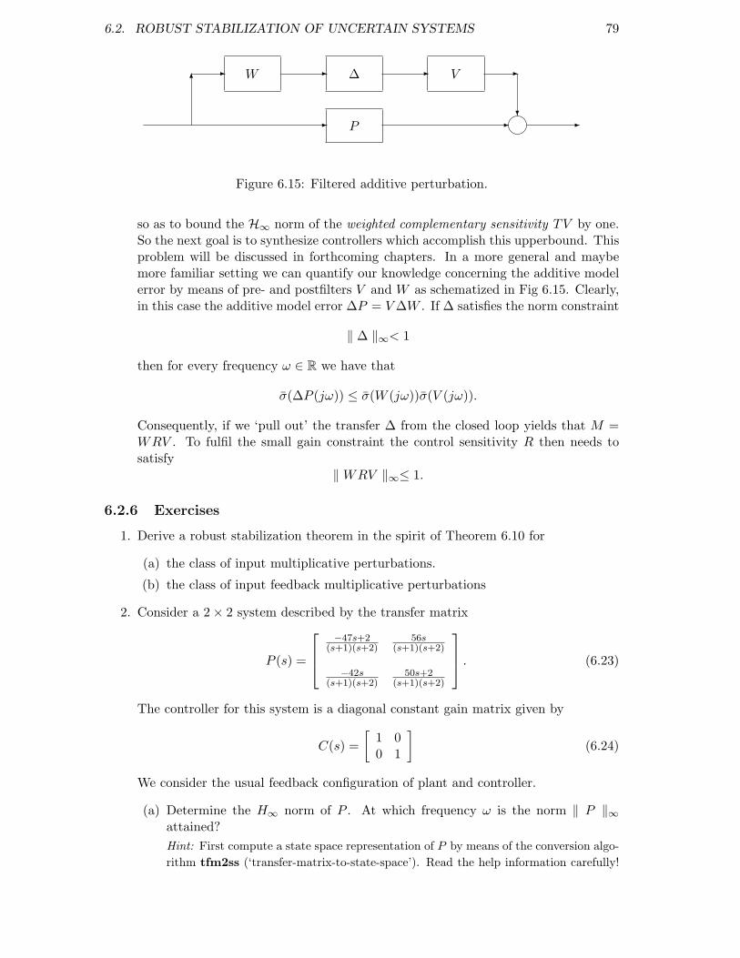
6.2. ROBUST STABILIZATION OF UNCERTAIN SYSTEMS 79
W ∆ V
P
Figure 6.15: Filtered additive perturbation.
so as to bound the H∞ norm of the weighted complementary sensitivity TV by one.So the next goal is to synthesize controllers which accomplish this upperbound. Thisproblem will be discussed in forthcoming chapters. In a more general and maybemore familiar setting we can quantify our knowledge concerning the additive modelerror by means of pre- and postfilters V and W as schematized in Fig 6.15. Clearly,in this case the additive model error ∆P = V∆W . If ∆ satisfies the norm constraint
‖ ∆ ‖∞< 1
then for every frequency ω ∈ R we have that
σ(∆P (jω)) ≤ σ(W (jω))σ(V (jω)).
Consequently, if we ‘pull out’ the transfer ∆ from the closed loop yields that M =WRV . To fulfil the small gain constraint the control sensitivity R then needs tosatisfy
‖WRV ‖∞≤ 1.
6.2.6 Exercises
1. Derive a robust stabilization theorem in the spirit of Theorem 6.10 for
(a) the class of input multiplicative perturbations.
(b) the class of input feedback multiplicative perturbations
2. Consider a 2× 2 system described by the transfer matrix
P (s) =
−47s+2
(s+1)(s+2)56s
(s+1)(s+2)
−42s(s+1)(s+2)
50s+2(s+1)(s+2)
. (6.23)
The controller for this system is a diagonal constant gain matrix given by
C(s) =[
1 00 1
](6.24)
We consider the usual feedback configuration of plant and controller.
(a) Determine the H∞ norm of P . At which frequency ω is the norm ‖ P ‖∞attained?Hint: First compute a state space representation of P by means of the conversion algo-rithm tfm2ss (‘transfer-matrix-to-state-space’). Read the help information carefully!
80 CHAPTER 6. WEIGHTING FILTERS
(The denominator polynomial is the same as in Exercise 2, the numerator polynomialsare represented in one matrix: the first row being [0 -47 2], the second [0 -42 0], etc.Once you have a state space representation of P you can read its H∞ norm from a plotof the singular values of P . Use the routine sigma.
(b) Use (6.24) as a controller for the plant P and plot the singular values of theclosed loop control-sensitivity C(I + PC)−1 to investigate robust stability ofthis system. Determine the robust stability margin of the closed loop systemunder additive perturbations of the plant.Hint: Use the MATLAB routine feedbk with the right ‘type’ option as in exercise 6.1to construct a state space representation of the control-sensitivity and use sigma toread H∞ norms of multivariable systems.
(c) Consider the perturbed controller
C(s) =[
1.13 00 .88
]and compute the closed-loop poles of this system. Conclusion?Hint: Use again the procedure feedbk to obtain a state space representation of theclosed loop system. Recall that the closed loop poles are the eigenvalues of the ‘A’matrix in any minimal representation of the closed loop system. See also the routineminreal.
3. Consider the linearized system of an unstable batch reactor described by the statespace model
x =
1.38 −0.2077 6.715 −5.676−0.5814 −4.29 0 0.6751.067 4.273 −6.654 5.8930.048 4.273 1.343 −2.104
x+
0 0
5.679 01.136 −3.1461.136 0
u
y =(
1 0 1 −10 1 0 0
)(a) Verify (using MATLAB!) that the input output system defined by this model
is unstable.
(b) Consider the controller with transfer function
C(s) =(
0 −25 0
)+
1s
(0 −28 0
)Using Matlab, interconnect the controller with the given plant and show thatthe corresponding closed loop system is stable.
(c) Make a plot of the singular values (as function of frequency) of the complemen-tary sensitivity PC(I + PC)−1 of the closed loop system.
(d) What are your conclusions concerning robust stability of the closed loop system?
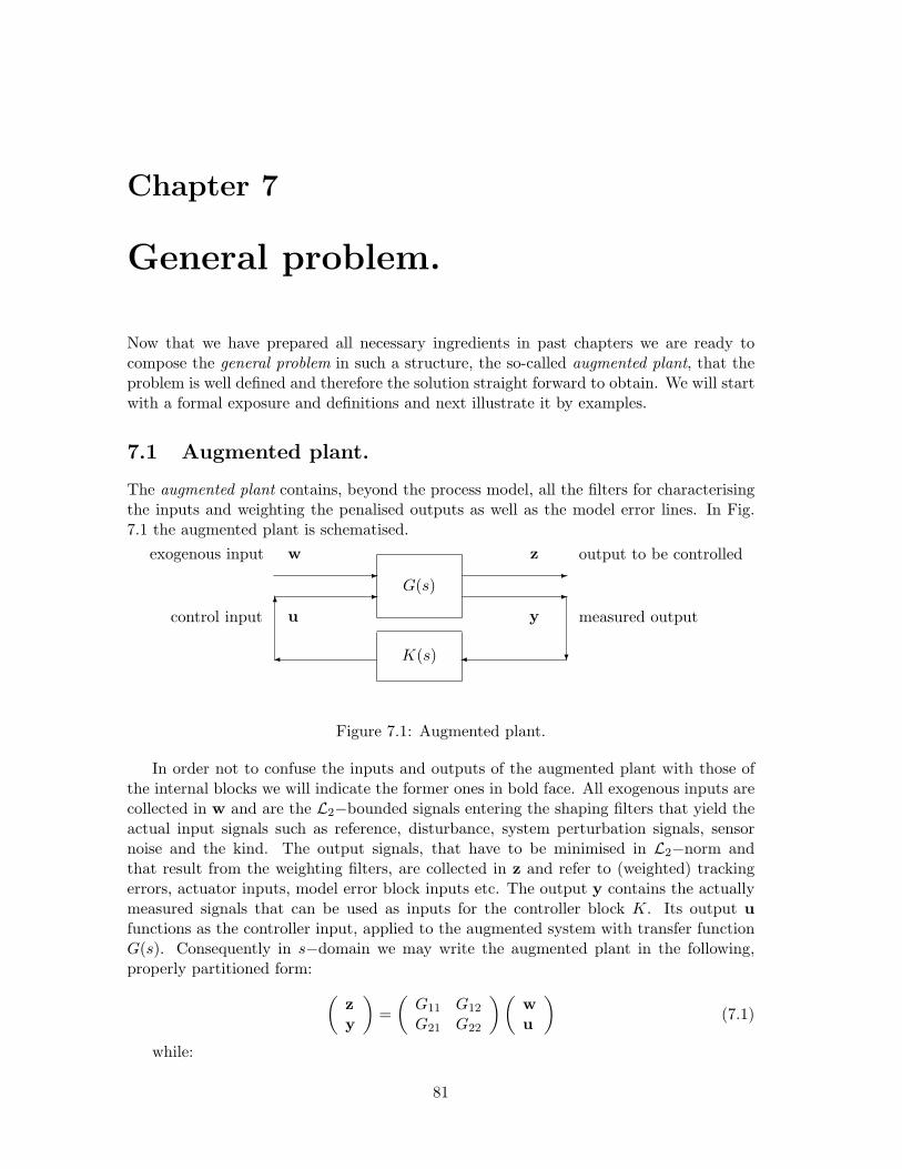
Chapter 7
General problem.
Now that we have prepared all necessary ingredients in past chapters we are ready tocompose the general problem in such a structure, the so-called augmented plant, that theproblem is well defined and therefore the solution straight forward to obtain. We will startwith a formal exposure and definitions and next illustrate it by examples.
7.1 Augmented plant.
The augmented plant contains, beyond the process model, all the filters for characterisingthe inputs and weighting the penalised outputs as well as the model error lines. In Fig.7.1 the augmented plant is schematised.
G(s)
K(s)
w z
u y
exogenous input
control input
output to be controlled
measured output
Figure 7.1: Augmented plant.
In order not to confuse the inputs and outputs of the augmented plant with those ofthe internal blocks we will indicate the former ones in bold face. All exogenous inputs arecollected in w and are the L2−bounded signals entering the shaping filters that yield theactual input signals such as reference, disturbance, system perturbation signals, sensornoise and the kind. The output signals, that have to be minimised in L2−norm andthat result from the weighting filters, are collected in z and refer to (weighted) trackingerrors, actuator inputs, model error block inputs etc. The output y contains the actuallymeasured signals that can be used as inputs for the controller block K. Its output ufunctions as the controller input, applied to the augmented system with transfer functionG(s). Consequently in s−domain we may write the augmented plant in the following,properly partitioned form: (
zy
)=(G11 G12G21 G22
)(wu
)(7.1)
while:
81
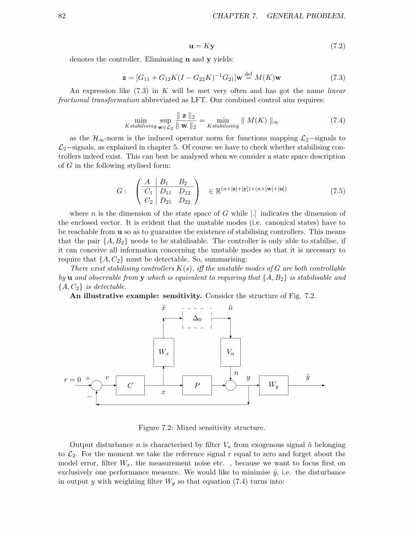
82 CHAPTER 7. GENERAL PROBLEM.
u = Ky (7.2)
denotes the controller. Eliminating u and y yields:
z = [G11 +G12K(I −G22K)−1G21]wdef= M(K)w (7.3)
An expression like (7.3) in K will be met very often and has got the name linearfractional transformation abbreviated as LFT. Our combined control aim requires:
minKstabilising
supw∈L2
‖ z ‖2‖ w ‖2 = min
Kstabilising‖M(K) ‖∞ (7.4)
as the H∞-norm is the induced operator norm for functions mapping L2−signals toL2−signals, as explained in chapter 5. Of course we have to check whether stabilising con-trollers indeed exist. This can best be analysed when we consider a state space descriptionof G in the following stylised form:
G :
A B1 B2
C1 D11 D12C2 D21 D22
∈ R(n+[z]+[y])×(n+[w]+[u]) (7.5)
where n is the dimension of the state space of G while [.] indicates the dimension ofthe enclosed vector. It is evident that the unstable modes (i.e. canonical states) have tobe reachable from u so as to guarantee the existence of stabilising controllers. This meansthat the pair A,B2 needs to be stabilisable. The controller is only able to stabilise, ifit can conceive all information concerning the unstable modes so that it is necessary torequire that A,C2 must be detectable. So, summarising:
There exist stabilising controllers K(s), iff the unstable modes of G are both controllableby u and observable from y which is equivalent to requiring that A,B2 is stabilisable andA,C2 is detectable.
An illustrative example: sensitivity. Consider the structure of Fig. 7.2.
C P Wy
Wx Vn
∆0
r = 0 +
−
e
x
y y
x n
n
Figure 7.2: Mixed sensitivity structure.
Output disturbance n is characterised by filter Vn from exogenous signal n belongingto L2. For the moment we take the reference signal r equal to zero and forget about themodel error, filter Wx, the measurement noise etc. , because we want to focus first onexclusively one performance measure. We would like to minimise y, i.e. the disturbancein output y with weighting filter Wy so that equation (7.4) turns into:
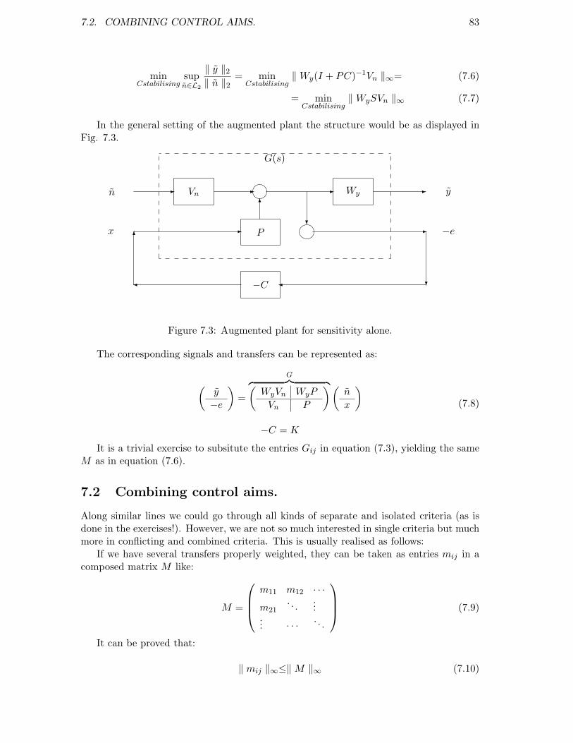
7.2. COMBINING CONTROL AIMS. 83
minCstabilising
supn∈L2
‖ y ‖2‖ n ‖2 = min
Cstabilising‖Wy(I + PC)−1Vn ‖∞= (7.6)
= minCstabilising
‖WySVn ‖∞ (7.7)
In the general setting of the augmented plant the structure would be as displayed inFig. 7.3.
−C
P
Vn Wy
G(s)
n
x
y
−e
Figure 7.3: Augmented plant for sensitivity alone.
The corresponding signals and transfers can be represented as:
(y
−e)
=
G︷ ︸︸ ︷(WyVn WyP
Vn P
)(n
x
)−C = K
(7.8)
It is a trivial exercise to subsitute the entries Gij in equation (7.3), yielding the sameM as in equation (7.6).
7.2 Combining control aims.
Along similar lines we could go through all kinds of separate and isolated criteria (as isdone in the exercises!). However, we are not so much interested in single criteria but muchmore in conflicting and combined criteria. This is usually realised as follows:
If we have several transfers properly weighted, they can be taken as entries mij in acomposed matrix M like:
M =
m11 m12 · · ·m21
. . ....
... · · · . . .
(7.9)
It can be proved that:
‖ mij ‖∞≤‖M ‖∞ (7.10)
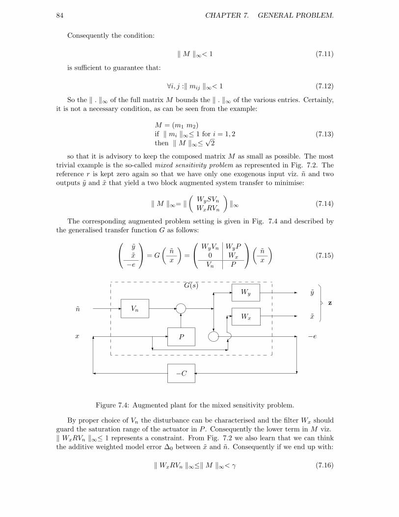
84 CHAPTER 7. GENERAL PROBLEM.
Consequently the condition:
‖M ‖∞< 1 (7.11)
is sufficient to guarantee that:
∀i, j :‖ mij ‖∞< 1 (7.12)
So the ‖ . ‖∞ of the full matrix M bounds the ‖ . ‖∞ of the various entries. Certainly,it is not a necessary condition, as can be seen from the example:
M = (m1 m2)if ‖ mi ‖∞≤ 1 for i = 1, 2then ‖M ‖∞≤
√2
(7.13)
so that it is advisory to keep the composed matrix M as small as possible. The mosttrivial example is the so-called mixed sensitivity problem as represented in Fig. 7.2. Thereference r is kept zero again so that we have only one exogenous input viz. n and twooutputs y and x that yield a two block augmented system transfer to minimise:
‖M ‖∞= ‖(WySVn
WxRVn
)‖∞ (7.14)
The corresponding augmented problem setting is given in Fig. 7.4 and described bythe generalised transfer function G as follows: y
x
−e
= G
(n
x
)=
WyVn WyP0 Wx
Vn P
(n
x
)(7.15)
−C
P
Vn
G(s)
n
x −e
Wy
Wx
y
x
z
Figure 7.4: Augmented plant for the mixed sensitivity problem.
By proper choice of Vn the disturbance can be characterised and the filter Wx shouldguard the saturation range of the actuator in P . Consequently the lower term in M viz.‖ WxRVn ‖∞≤ 1 represents a constraint. From Fig. 7.2 we also learn that we can thinkthe additive weighted model error ∆0 between x and n. Consequently if we end up with:
‖WxRVn ‖∞≤‖M ‖∞< γ (7.16)
7.3. MIXED SENSITIVITY PROBLEM. 85
we can guarantee robust stability for:
‖ V −1n ∆PWx
−1 ‖∞=‖ ∆0 ‖∞< 1/γ (7.17)
or equivalently:
∀ω ∈ R : |∆P (jω)| < |Vn(jω)||Wx(jω)|/γ (7.18)
So by proper choice of Vn and Wx we can combine saturation and robust stability.Finally, by the filter Wy we put our requirements on the band, for which the disturbanceshould be removed, leading to the first term WySVn. So here we have a mixed sensitivitycriterion in M , where the lower term puts a constraint in terms of the control sensitivity,while the upper term aims for a high performance in terms of the sensitivity.
7.3 Mixed sensitivity problem.
In general, such a mixed sensitivity can be described as:∣∣∣∣∣∣∣∣ W1SV1W2NV2
∣∣∣∣∣∣∣∣∞
←←
performancerobustness
(7.19)
In the lower term robustness is guarded by N which is either T or R. It can in factalways supposed to be T , as the difference with R is only inthe weighting by P that canbe brought into the weighting filters W2 and V2. As the lower term puts a hard constraintwhile the upper term is a control aim that should be optimised under the lower constraint,the general way, to solve this, runs along the following lines:
1. Choose weights W2 and V2 such that robustness is obtained for:
‖W2NV2 ‖∞< 1. (7.20)
2. Choose W1 and V1 for the expected, obtainable performance.
3. Compute a stabilising controller C (see chapter 13) such that:∣∣∣∣∣∣∣∣ W1SV1W2NV2
∣∣∣∣∣∣∣∣∞< γ (7.21)
where γ is as small as possible.
4. If γ > 1, decrease W1 and/or V1 in gain and/or frequency band in order to relax theperformance aim and thereby giving more room to satisfy the robustness constraint.Go back to step 3.
5. If γ < 1−ε, where ε is some small number, based on desired and obtainable numericalaccuracy, there is obviously some room left for improving the performance so that wemay tighten the weights W1 and V1 by increasing gains and/or bands. Next repeatstep 3.
6. If 1− ε < γ < 1 stop the above iteration process and evaluate the result by studyingthe Bode plots of S and N , step responses, simulations and watching possible actu-ator saturation. If the result is not satisfactory, repeat above iteration process afterhaving adjusted the weighting filters.
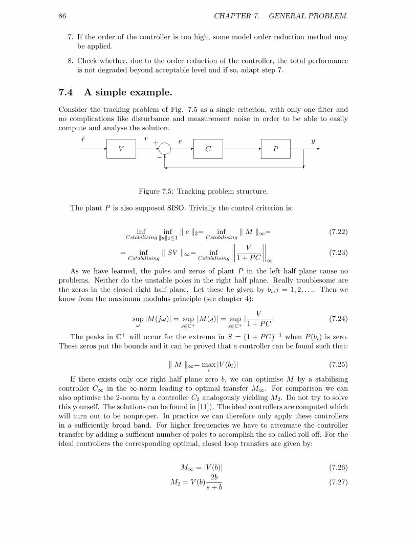
86 CHAPTER 7. GENERAL PROBLEM.
7. If the order of the controller is too high, some model order reduction method maybe applied.
8. Check whether, due to the order reduction of the controller, the total performanceis not degraded beyond acceptable level and if so, adapt step 7.
7.4 A simple example.
Consider the tracking problem of Fig. 7.5 as a single criterion, with only one filter andno complications like disturbance and measurement noise in order to be able to easilycompute and analyse the solution.
V C P
r r +
−
e y
Figure 7.5: Tracking problem structure.
The plant P is also supposed SISO. Trivially the control criterion is:
infCstabilising
inf‖u‖2≤1
‖ e ‖2= infCstabilising
‖M ‖∞= (7.22)
= infCstabilising
‖ SV ‖∞= infCstabilising
∣∣∣∣∣∣∣∣ V
1 + PC
∣∣∣∣∣∣∣∣∞
(7.23)
As we have learned, the poles and zeros of plant P in the left half plane cause noproblems. Neither do the unstable poles in the right half plane. Really troublesome arethe zeros in the closed right half plane. Let these be given by bi, i = 1, 2, . . .. Then weknow from the maximum modulus principle (see chapter 4):
supω|M(jω)| = sup
s∈C+|M(s)| = sup
s∈C+| V
1 + PC| (7.24)
The peaks in C+ will occur for the extrema in S = (1 + PC)−1 when P (bi) is zero.These zeros put the bounds and it can be proved that a controller can be found such that:
‖M ‖∞= maxi|V (bi)| (7.25)
If there exists only one right half plane zero b, we can optimise M by a stabilisingcontroller C∞ in the ∞-norm leading to optimal transfer M∞. For comparison we canalso optimise the 2-norm by a controller C2 analogously yielding M2. Do not try to solvethis yourself. The solutions can be found in [11]). The ideal controllers are computed whichwill turn out to be nonproper. In practice we can therefore only apply these controllersin a sufficiently broad band. For higher frequencies we have to attenuate the controllertransfer by adding a sufficient number of poles to accomplish the so-called roll-off. For theideal controllers the corresponding optimal, closed loop transfers are given by:
M∞ = |V (b)| (7.26)
M2 = V (b)2bs+ b
(7.27)
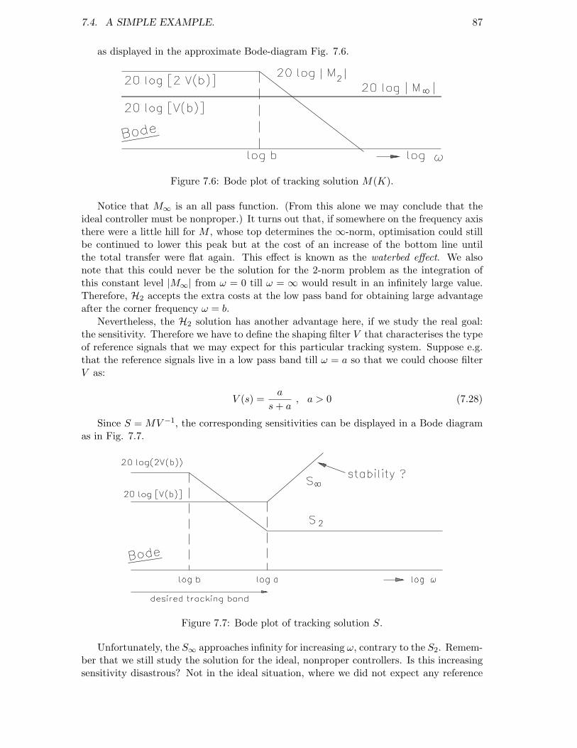
7.4. A SIMPLE EXAMPLE. 87
as displayed in the approximate Bode-diagram Fig. 7.6.
Figure 7.6: Bode plot of tracking solution M(K).
Notice that M∞ is an all pass function. (From this alone we may conclude that theideal controller must be nonproper.) It turns out that, if somewhere on the frequency axisthere were a little hill for M , whose top determines the ∞-norm, optimisation could stillbe continued to lower this peak but at the cost of an increase of the bottom line untilthe total transfer were flat again. This effect is known as the waterbed effect. We alsonote that this could never be the solution for the 2-norm problem as the integration ofthis constant level |M∞| from ω = 0 till ω = ∞ would result in an infinitely large value.Therefore, H2 accepts the extra costs at the low pass band for obtaining large advantageafter the corner frequency ω = b.
Nevertheless, the H2 solution has another advantage here, if we study the real goal:the sensitivity. Therefore we have to define the shaping filter V that characterises the typeof reference signals that we may expect for this particular tracking system. Suppose e.g.that the reference signals live in a low pass band till ω = a so that we could choose filterV as:
V (s) =a
s+ a, a > 0 (7.28)
Since S = MV −1, the corresponding sensitivities can be displayed in a Bode diagramas in Fig. 7.7.
Figure 7.7: Bode plot of tracking solution S.
Unfortunately, the S∞ approaches infinity for increasing ω, contrary to the S2. Remem-ber that we still study the solution for the ideal, nonproper controllers. Is this increasingsensitivity disastrous? Not in the ideal situation, where we did not expect any reference
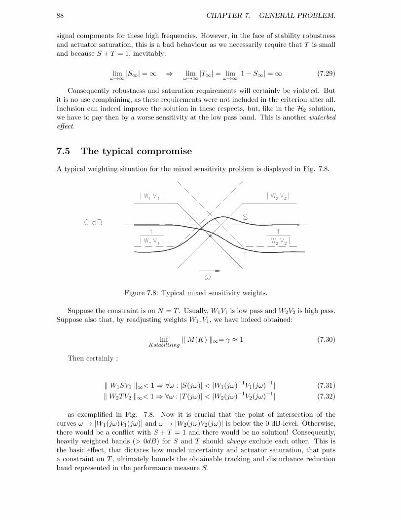
88 CHAPTER 7. GENERAL PROBLEM.
signal components for these high frequencies. However, in the face of stability robustnessand actuator saturation, this is a bad behaviour as we necessarily require that T is smalland because S + T = 1, inevitably:
limω→∞ |S∞| =∞ ⇒ lim
ω→∞ |T∞| = limω→∞ |1− S∞| =∞ (7.29)
Consequently robustness and saturation requirements will certainly be violated. Butit is no use complaining, as these requirements were not included in the criterion after all.Inclusion can indeed improve the solution in these respects, but, like in the H2 solution,we have to pay then by a worse sensitivity at the low pass band. This is another waterbedeffect.
7.5 The typical compromise
A typical weighting situation for the mixed sensitivity problem is displayed in Fig. 7.8.
Figure 7.8: Typical mixed sensitivity weights.
Suppose the constraint is on N = T . Usually, W1V1 is low pass and W2V2 is high pass.Suppose also that, by readjusting weights W1, V1, we have indeed obtained:
infKstabilising
‖M(K) ‖∞= γ ≈ 1 (7.30)
Then certainly :
‖W1SV1 ‖∞< 1⇒ ∀ω : |S(jω)| < |W1(jω)−1V1(jω)−1| (7.31)‖W2TV2 ‖∞< 1⇒ ∀ω : |T (jω)| < |W2(jω)−1V2(jω)−1| (7.32)
as exemplified in Fig. 7.8. Now it is crucial that the point of intersection of thecurves ω → |W1(jω)V1(jω)| and ω → |W2(jω)V2(jω)| is below the 0 dB-level. Otherwise,there would be a conflict with S + T = 1 and there would be no solution! Consequently,heavily weighted bands (> 0dB) for S and T should always exclude each other. This isthe basic effect, that dictates how model uncertainty and actuator saturation, that putsa constraint on T , ultimately bounds the obtainable tracking and disturbance reductionband represented in the performance measure S.
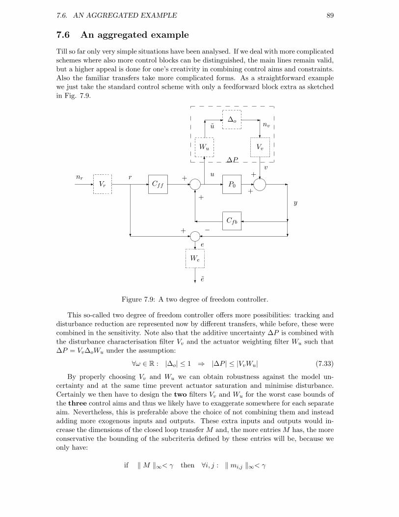
7.6. AN AGGREGATED EXAMPLE 89
7.6 An aggregated example
Till so far only very simple situations have been analysed. If we deal with more complicatedschemes where also more control blocks can be distinguished, the main lines remain valid,but a higher appeal is done for one’s creativity in combining control aims and constraints.Also the familiar transfers take more complicated forms. As a straightforward examplewe just take the standard control scheme with only a feedforward block extra as sketchedin Fig. 7.9.
Cfb
P0CffVr
Wu Vv
We
nr r u
u nv
v
y
e
e
+
++
+
+ −
∆o
∆P
Figure 7.9: A two degree of freedom controller.
This so-called two degree of freedom controller offers more possibilities: tracking anddisturbance reduction are represented now by different transfers, while before, these werecombined in the sensitivity. Note also that the additive uncertainty ∆P is combined withthe disturbance characterisation filter Vv and the actuator weighting filter Wu such that∆P = Vv∆oWu under the assumption:
∀ω ∈ R : |∆o| ≤ 1 ⇒ |∆P | ≤ |VvWu| (7.33)
By properly choosing Vv and Wu we can obtain robustness against the model un-certainty and at the same time prevent actuator saturation and minimise disturbance.Certainly we then have to design the two filters Vv and Wu for the worst case bounds ofthe three control aims and thus we likely have to exaggerate somewhere for each separateaim. Nevertheless, this is preferable above the choice of not combining them and insteadadding more exogenous inputs and outputs. These extra inputs and outputs would in-crease the dimensions of the closed loop transfer M and, the more entries M has, the moreconservative the bounding of the subcriteria defined by these entries will be, because weonly have:
if ‖M ‖∞< γ then ∀i, j : ‖ mi,j ‖∞< γ
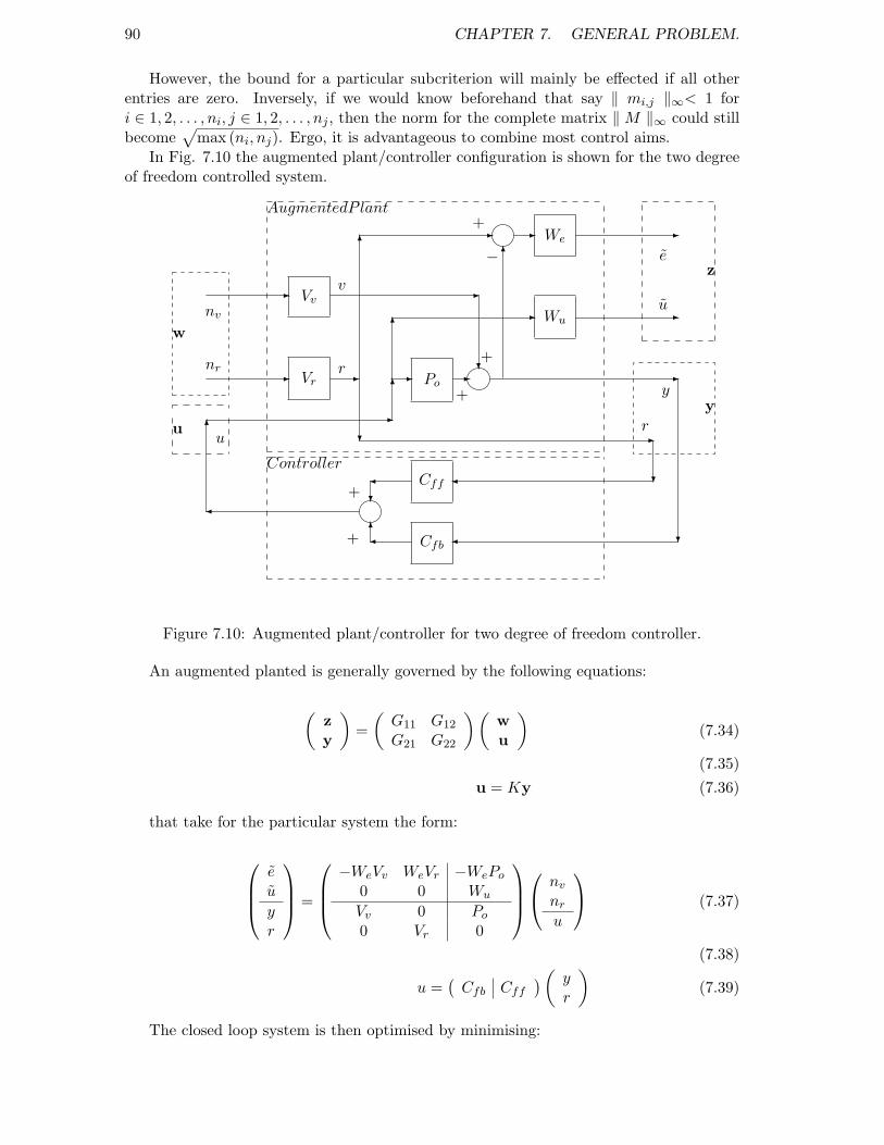
90 CHAPTER 7. GENERAL PROBLEM.
However, the bound for a particular subcriterion will mainly be effected if all otherentries are zero. Inversely, if we would know beforehand that say ‖ mi,j ‖∞< 1 fori ∈ 1, 2, . . . , ni, j ∈ 1, 2, . . . , nj , then the norm for the complete matrix ‖M ‖∞ could stillbecome
√max (ni, nj). Ergo, it is advantageous to combine most control aims.
In Fig. 7.10 the augmented plant/controller configuration is shown for the two degreeof freedom controlled system.
Cfb
Cff
PoVr
Vv
Wu
We
AugmentedP lant
Controller
nv
nr
u
w
ze
uv
r
+
−
+
+
+
+
y
r
yu
Figure 7.10: Augmented plant/controller for two degree of freedom controller.
An augmented planted is generally governed by the following equations:
(zy
)=(G11 G12G21 G22
)(wu
)(7.34)
(7.35)u = Ky (7.36)
that take for the particular system the form:
eu
yr
=
−WeVv WeVr −WePo
0 0 Wu
Vv 0 Po
0 Vr 0
nv
nr
u
(7.37)
(7.38)
u =(Cfb Cff
)( yr
)(7.39)
The closed loop system is then optimised by minimising:
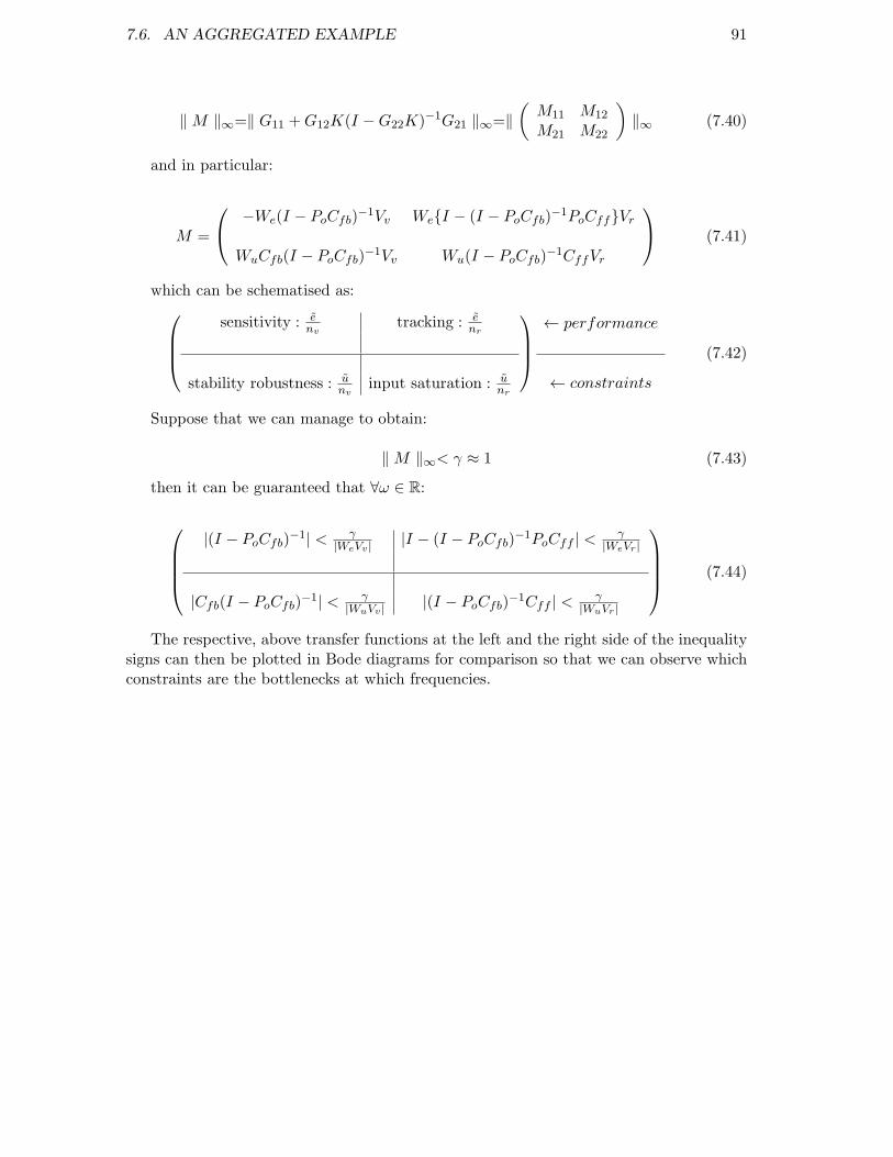
7.6. AN AGGREGATED EXAMPLE 91
‖M ‖∞=‖ G11 +G12K(I −G22K)−1G21 ‖∞=‖(M11 M12M21 M22
)‖∞ (7.40)
and in particular:
M =
−We(I − PoCfb)−1Vv WeI − (I − PoCfb)−1PoCffVr
WuCfb(I − PoCfb)−1Vv Wu(I − PoCfb)−1CffVr
(7.41)
which can be schematised as:sensitivity : e
nvtracking : e
nr
stability robustness : unv
input saturation : unr
← performance
← constraints
(7.42)
Suppose that we can manage to obtain:
‖M ‖∞< γ ≈ 1 (7.43)
then it can be guaranteed that ∀ω ∈ R:
|(I − PoCfb)−1| < γ
|WeVv | |I − (I − PoCfb)−1PoCff | < γ|WeVr|
|Cfb(I − PoCfb)−1| < γ|WuVv | |(I − PoCfb)−1Cff | < γ
|WuVr|
(7.44)
The respective, above transfer functions at the left and the right side of the inequalitysigns can then be plotted in Bode diagrams for comparison so that we can observe whichconstraints are the bottlenecks at which frequencies.

92 CHAPTER 7. GENERAL PROBLEM.
7.7 Exercise
Vr C P Wy
We Wx Wz Vξ
r
e x z ξ
y
y
r e x zn
+ –
+
+
For the given blockscheme we consider first SISO-transfers from a certain input to acertain output. It is asked to compute the linear fractional transfer, to explain the use ofthe particular transfer, to name it (if possible) and finally to give the augmented plant inblockscheme and express the matrix transfer G. Train yourself for the following transfers:
a) from ξ to y (see example ‘sensitivity’ in lecture notes)
b) from r to e
c) from ξ to z (two goals!)
d) from ξ to x (two goals!)
The same for the following MIMO-transfers:
e) from ξ to y and z (three goals!)
We now split the previously combined inputs in ξ into two inputs ξ1 and ξ2 with respectiveshaping filters V1 and V2:
f) from ξ1 and ξ2 to y and z.
Also for the next scheme:
Vr C1 P
C2
We
Wx
r r +
+
x y –
+
e
x
e
g) from r to x and e.
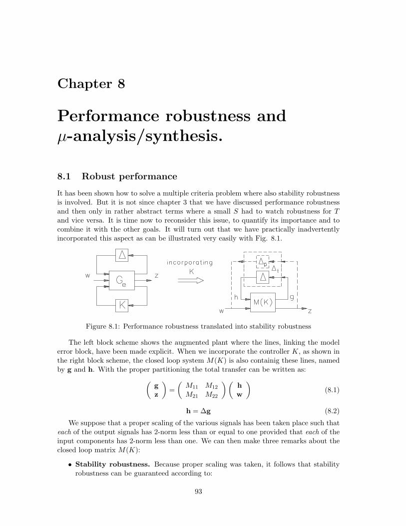
Chapter 8
Performance robustness andµ-analysis/synthesis.
8.1 Robust performance
It has been shown how to solve a multiple criteria problem where also stability robustnessis involved. But it is not since chapter 3 that we have discussed performance robustnessand then only in rather abstract terms where a small S had to watch robustness for Tand vice versa. It is time now to reconsider this issue, to quantify its importance and tocombine it with the other goals. It will turn out that we have practically inadvertentlyincorporated this aspect as can be illustrated very easily with Fig. 8.1.
Figure 8.1: Performance robustness translated into stability robustness
The left block scheme shows the augmented plant where the lines, linking the modelerror block, have been made explicit. When we incorporate the controller K, as shown inthe right block scheme, the closed loop system M(K) is also containig these lines, namedby g and h. With the proper partitioning the total transfer can be written as:(
gz
)=(M11 M12M21 M22
)(hw
)(8.1)
h = ∆g (8.2)
We suppose that a proper scaling of the various signals has been taken place such thateach of the output signals has 2-norm less than or equal to one provided that each of theinput components has 2-norm less than one. We can then make three remarks about theclosed loop matrix M(K):
• Stability robustness. Because proper scaling was taken, it follows that stabilityrobustness can be guaranteed according to:
93

94CHAPTER 8. PERFORMANCE ROBUSTNESS AND µ-ANALYSIS/SYNTHESIS.
‖ ∆ ‖∞≤ 1 ∩ ‖M11(K) ‖∞< 1 (8.3)
So the ∞-norm of M11 determines robust stability.
• Nominal performance. Without model errors taken into account (i.e. ∆=0 andthus h=0) ‖ z ‖2 can be kept less than 1 provided that:
‖M22(K) ‖∞< 1 (8.4)
So the ∞-norm of M22 determines nominal performance.
This condition can be unambiguously translated into a stability condition, like forstability robustness, by introducing a fancy feedback over a fancy block ∆p as:
w = ∆pz : ‖ ∆p ‖∞≤ 1 ∩ ‖M22(K) ‖∞< 1 (8.5)
There is now a complete symmetry and similarity in the two separate loops over ∆and ∆p.
• Robust performance. For robust performance we have to guarantee that z staysbelow 1 irrespective of the model errors. That is, in the face of a signal h unequalto zero and ‖ h ‖2≤ 1, we require ‖ z ‖2< 1. If we now require that:
‖M(K) ‖∞< 1 (8.6)
we have a sufficient condition to guarantee that the performance is robust.
proof: From equation 8.6 we have:∣∣∣∣∣∣∣∣ gz
∣∣∣∣∣∣∣∣2<
∣∣∣∣∣∣∣∣ hw
∣∣∣∣∣∣∣∣2
(8.7)
From ‖ ∆ ‖∞≤ 1 we may state:
‖ h ‖2≤‖ g ‖2 (8.8)
Combination with the first inequality yields:∣∣∣∣∣∣∣∣ gz
∣∣∣∣∣∣∣∣2<
∣∣∣∣∣∣∣∣ gw
∣∣∣∣∣∣∣∣2
(8.9)
so that indeed:
‖ z ‖2<‖ w ‖2≤ 1 (8.10)
which ends the proof.
Of course robust stability and nominal performance is implied as:
‖M ‖∞< 1 ⇒ ‖M11 ‖∞< 1 and ‖M22 ‖∞< 1 (8.11)
8.2. NO PERFORMANCE ROBUSTNESS FOR THE MIXED SENSITIVITY STRUCTURE.95
But we also obtain that ‖ z ‖2< 1 for all allowed ‖ ∆ ‖∞≤ 1. Thus performancerobustness is guaranteed. Ergo, inadvertently, we combined stability robustness andnominal performance in the above structure and we automatically receive perfor-mance robustness almost as a spin off!
8.2 No performance robustness for the mixed sensitivitystructure.
Unfortunately, the performance robustness, as derived in the previous section, only holdsfor the so called four block problem, where:
M =(M11 M12M21 M22
)(8.12)
If M12 and M21 do not exist in two block problems:
M =(M11 M22
)or M =
(M11M22
)(8.13)
the robust performance property is lost (see for yourself if you try to proof it along thelines of the previous section).
Consequently the earlier proposed mixed sensitivity problem:
M =(
WS(I + PC)−1VWRC(I + PC)−1V
)(8.14)
lacks robust performance. It turns out that the resulting controller simply com-pensates the stable poles and zeros of the plant (model) P. (see Smit [19]) It can easily beunderstood, that this will be a bad solution if the plant has poles and zeros close to theinstability border: the imaginary axis. Small deviations of the real plant from its modelwill soon deteriorate the performance: the intended pole-zero cancellations will not beperfect and the rootlocus will show small excursions close to the imaginary axis causingsharp resonance peaks in the closed loop Bode-plots.
8.3 µ-analysis
We could be very satisfied with the general result of section 8.1, but there is an annoyingaspect in the sufficiency of the condition (8.6). This condition asks more than is strictlynecessary. This can be understood, if we translate this condition into a stability condition,as we did for the nominal performance. Then condition (8.6) provides robust stability evenif ∆t is a full block, i.e. all its entries may be nonzero. It means that h may also dependon z and that w may also depend on g. As there are no such relations, we required toomuch. We know that ∆t is not a full block but:
∆t =(
∆ 00 ∆p
)(8.15)
So we passed over the diagonal structure of the total ∆t-block. The off-diagonal zerosindicate that the performance output z has no influence whatsoever onto the model erroroutput h and reciprocally the model error input line g won’t affect the exogenous inputsw . Ergo, condition (8.6) is too strong and introduces conservatism.
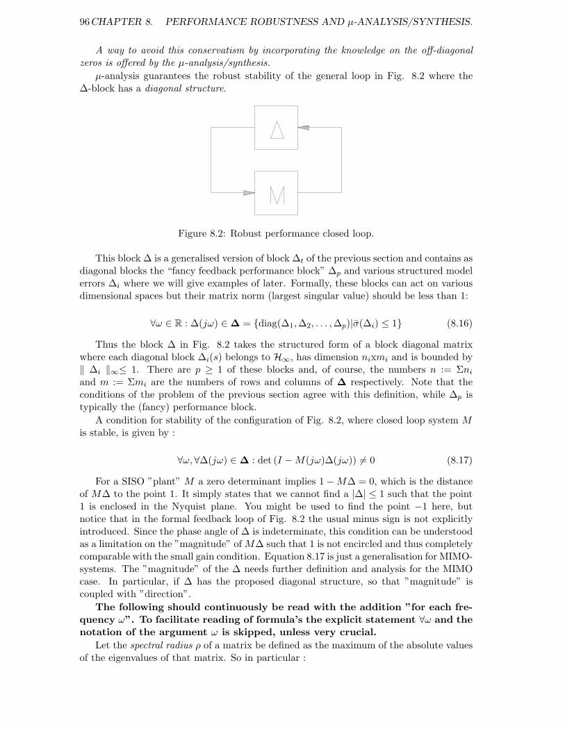
96CHAPTER 8. PERFORMANCE ROBUSTNESS AND µ-ANALYSIS/SYNTHESIS.
A way to avoid this conservatism by incorporating the knowledge on the off-diagonalzeros is offered by the µ-analysis/synthesis.
µ-analysis guarantees the robust stability of the general loop in Fig. 8.2 where the∆-block has a diagonal structure.
Figure 8.2: Robust performance closed loop.
This block ∆ is a generalised version of block ∆t of the previous section and contains asdiagonal blocks the “fancy feedback performance block” ∆p and various structured modelerrors ∆i where we will give examples of later. Formally, these blocks can act on variousdimensional spaces but their matrix norm (largest singular value) should be less than 1:
∀ω ∈ R : ∆(jω) ∈∆ = diag(∆1,∆2, . . . ,∆p)|σ(∆i) ≤ 1 (8.16)
Thus the block ∆ in Fig. 8.2 takes the structured form of a block diagonal matrixwhere each diagonal block ∆i(s) belongs to H∞, has dimension nixmi and is bounded by‖ ∆i ‖∞≤ 1. There are p ≥ 1 of these blocks and, of course, the numbers n := Σni
and m := Σmi are the numbers of rows and columns of ∆ respectively. Note that theconditions of the problem of the previous section agree with this definition, while ∆p istypically the (fancy) performance block.
A condition for stability of the configuration of Fig. 8.2, where closed loop system Mis stable, is given by :
∀ω, ∀∆(jω) ∈∆ : det (I −M(jω)∆(jω)) = 0 (8.17)
For a SISO ”plant” M a zero determinant implies 1−M∆ = 0, which is the distanceof M∆ to the point 1. It simply states that we cannot find a |∆| ≤ 1 such that the point1 is enclosed in the Nyquist plane. You might be used to find the point −1 here, butnotice that in the formal feedback loop of Fig. 8.2 the usual minus sign is not explicitlyintroduced. Since the phase angle of ∆ is indeterminate, this condition can be understoodas a limitation on the ”magnitude” of M∆ such that 1 is not encircled and thus completelycomparable with the small gain condition. Equation 8.17 is just a generalisation for MIMO-systems. The ”magnitude” of the ∆ needs further definition and analysis for the MIMOcase. In particular, if ∆ has the proposed diagonal structure, so that ”magnitude” iscoupled with ”direction”.
The following should continuously be read with the addition ”for each fre-quency ω”. To facilitate reading of formula’s the explicit statement ∀ω and thenotation of the argument ω is skipped, unless very crucial.
Let the spectral radius ρ of a matrix be defined as the maximum of the absolute valuesof the eigenvalues of that matrix. So in particular :
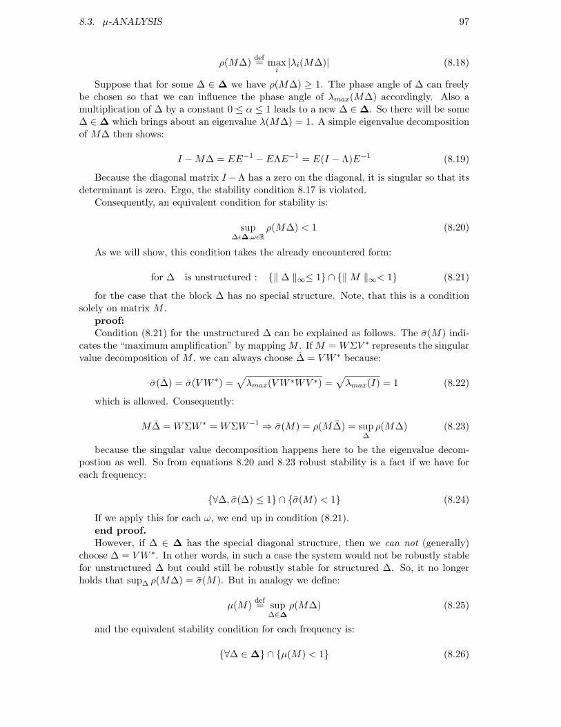
8.3. µ-ANALYSIS 97
ρ(M∆) def= maxi|λi(M∆)| (8.18)
Suppose that for some ∆ ∈ ∆ we have ρ(M∆) ≥ 1. The phase angle of ∆ can freelybe chosen so that we can influence the phase angle of λmax(M∆) accordingly. Also amultiplication of ∆ by a constant 0 ≤ α ≤ 1 leads to a new ∆ ∈∆. So there will be some∆ ∈∆ which brings about an eigenvalue λ(M∆) = 1. A simple eigenvalue decompositionof M∆ then shows:
I −M∆ = EE−1 − EΛE−1 = E(I − Λ)E−1 (8.19)
Because the diagonal matrix I −Λ has a zero on the diagonal, it is singular so that itsdeterminant is zero. Ergo, the stability condition 8.17 is violated.
Consequently, an equivalent condition for stability is:
sup∆ε∆,ωεR
ρ(M∆) < 1 (8.20)
As we will show, this condition takes the already encountered form:
for ∆ is unstructured : ‖ ∆ ‖∞≤ 1 ∩ ‖M ‖∞< 1 (8.21)
for the case that the block ∆ has no special structure. Note, that this is a conditionsolely on matrix M .
proof:Condition (8.21) for the unstructured ∆ can be explained as follows. The σ(M) indi-
cates the “maximum amplification” by mappingM . If M = WΣV ∗ represents the singularvalue decomposition of M , we can always choose ∆ = VW ∗ because:
σ(∆) = σ(VW ∗) =√λmax(VW ∗WV ∗) =
√λmax(I) = 1 (8.22)
which is allowed. Consequently:
M∆ = WΣW ∗ = WΣW−1 ⇒ σ(M) = ρ(M∆) = sup∆ρ(M∆) (8.23)
because the singular value decomposition happens here to be the eigenvalue decom-postion as well. So from equations 8.20 and 8.23 robust stability is a fact if we have foreach frequency:
∀∆, σ(∆) ≤ 1 ∩ σ(M) < 1 (8.24)
If we apply this for each ω, we end up in condition (8.21).end proof.However, if ∆ ∈ ∆ has the special diagonal structure, then we can not (generally)
choose ∆ = VW ∗. In other words, in such a case the system would not be robustly stablefor unstructured ∆ but could still be robustly stable for structured ∆. So, it no longerholds that sup∆ ρ(M∆) = σ(M). But in analogy we define:
µ(M) def= sup∆∈∆
ρ(M∆) (8.25)
and the equivalent stability condition for each frequency is:
∀∆ ∈∆ ∩ µ(M) < 1 (8.26)
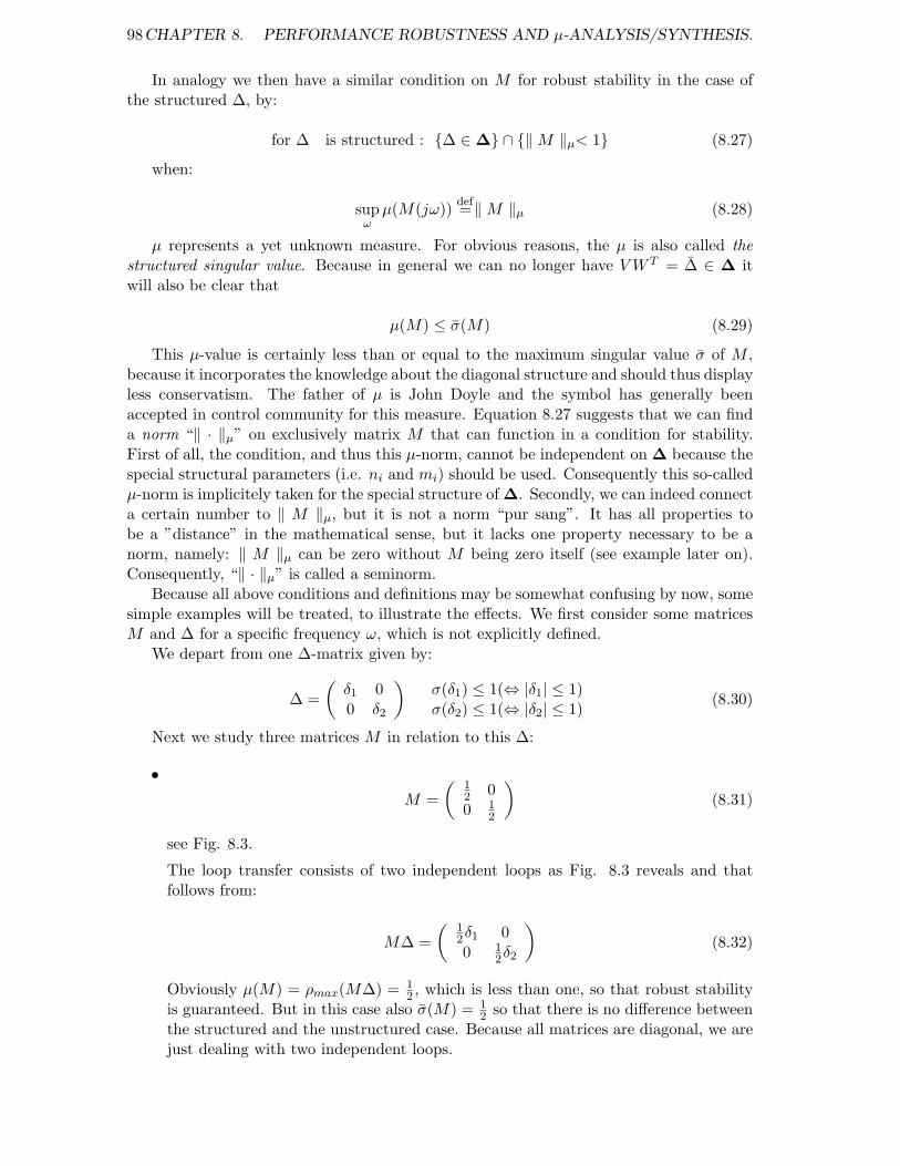
98CHAPTER 8. PERFORMANCE ROBUSTNESS AND µ-ANALYSIS/SYNTHESIS.
In analogy we then have a similar condition on M for robust stability in the case ofthe structured ∆, by:
for ∆ is structured : ∆ ∈∆ ∩ ‖M ‖µ< 1 (8.27)
when:
supωµ(M(jω)) def=‖M ‖µ (8.28)
µ represents a yet unknown measure. For obvious reasons, the µ is also called thestructured singular value. Because in general we can no longer have VW T = ∆ ∈ ∆ itwill also be clear that
µ(M) ≤ σ(M) (8.29)
This µ-value is certainly less than or equal to the maximum singular value σ of M ,because it incorporates the knowledge about the diagonal structure and should thus displayless conservatism. The father of µ is John Doyle and the symbol has generally beenaccepted in control community for this measure. Equation 8.27 suggests that we can finda norm “‖ · ‖µ” on exclusively matrix M that can function in a condition for stability.First of all, the condition, and thus this µ-norm, cannot be independent on ∆ because thespecial structural parameters (i.e. ni and mi) should be used. Consequently this so-calledµ-norm is implicitely taken for the special structure of ∆. Secondly, we can indeed connecta certain number to ‖ M ‖µ, but it is not a norm “pur sang”. It has all properties tobe a ”distance” in the mathematical sense, but it lacks one property necessary to be anorm, namely: ‖ M ‖µ can be zero without M being zero itself (see example later on).Consequently, “‖ · ‖µ” is called a seminorm.
Because all above conditions and definitions may be somewhat confusing by now, somesimple examples will be treated, to illustrate the effects. We first consider some matricesM and ∆ for a specific frequency ω, which is not explicitly defined.
We depart from one ∆-matrix given by:
∆ =(δ1 00 δ2
)σ(δ1) ≤ 1(⇔ |δ1| ≤ 1)σ(δ2) ≤ 1(⇔ |δ2| ≤ 1)
(8.30)
Next we study three matrices M in relation to this ∆:
•M =
( 12 00 1
2
)(8.31)
see Fig. 8.3.
The loop transfer consists of two independent loops as Fig. 8.3 reveals and thatfollows from:
M∆ =( 1
2δ1 00 1
2δ2
)(8.32)
Obviously µ(M) = ρmax(M∆) = 12 , which is less than one, so that robust stability
is guaranteed. But in this case also σ(M) = 12 so that there is no difference between
the structured and the unstructured case. Because all matrices are diagonal, we arejust dealing with two independent loops.
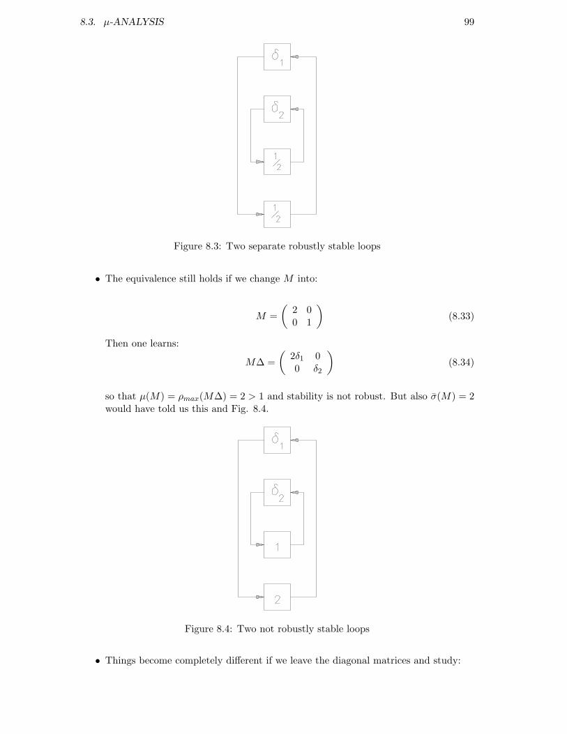
8.3. µ-ANALYSIS 99
Figure 8.3: Two separate robustly stable loops
• The equivalence still holds if we change M into:
M =(
2 00 1
)(8.33)
Then one learns:
M∆ =(
2δ1 00 δ2
)(8.34)
so that µ(M) = ρmax(M∆) = 2 > 1 and stability is not robust. But also σ(M) = 2would have told us this and Fig. 8.4.
Figure 8.4: Two not robustly stable loops
• Things become completely different if we leave the diagonal matrices and study:
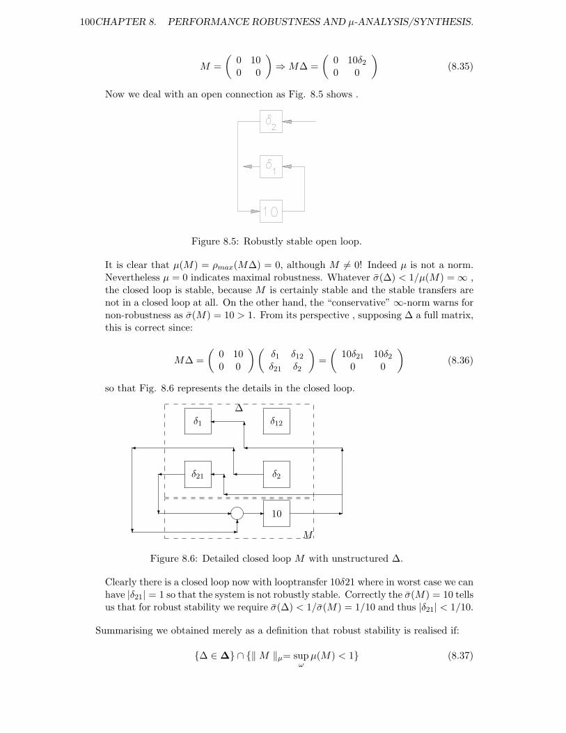
100CHAPTER 8. PERFORMANCE ROBUSTNESS AND µ-ANALYSIS/SYNTHESIS.
M =(
0 100 0
)⇒M∆ =
(0 10δ20 0
)(8.35)
Now we deal with an open connection as Fig. 8.5 shows .
Figure 8.5: Robustly stable open loop.
It is clear that µ(M) = ρmax(M∆) = 0, although M = 0! Indeed µ is not a norm.Nevertheless µ = 0 indicates maximal robustness. Whatever σ(∆) < 1/µ(M) =∞ ,the closed loop is stable, because M is certainly stable and the stable transfers arenot in a closed loop at all. On the other hand, the “conservative”∞-norm warns fornon-robustness as σ(M) = 10 > 1. From its perspective , supposing ∆ a full matrix,this is correct since:
M∆ =(
0 100 0
)(δ1 δ12δ21 δ2
)=(
10δ21 10δ20 0
)(8.36)
so that Fig. 8.6 represents the details in the closed loop.
δ21 δ2
δ1 δ12
10
∆
M
Figure 8.6: Detailed closed loop M with unstructured ∆.
Clearly there is a closed loop now with looptransfer 10δ21 where in worst case we canhave |δ21| = 1 so that the system is not robustly stable. Correctly the σ(M) = 10 tellsus that for robust stability we require σ(∆) < 1/σ(M) = 1/10 and thus |δ21| < 1/10.
Summarising we obtained merely as a definition that robust stability is realised if:
∆ ∈∆ ∩ ‖M ‖µ= supωµ(M) < 1 (8.37)
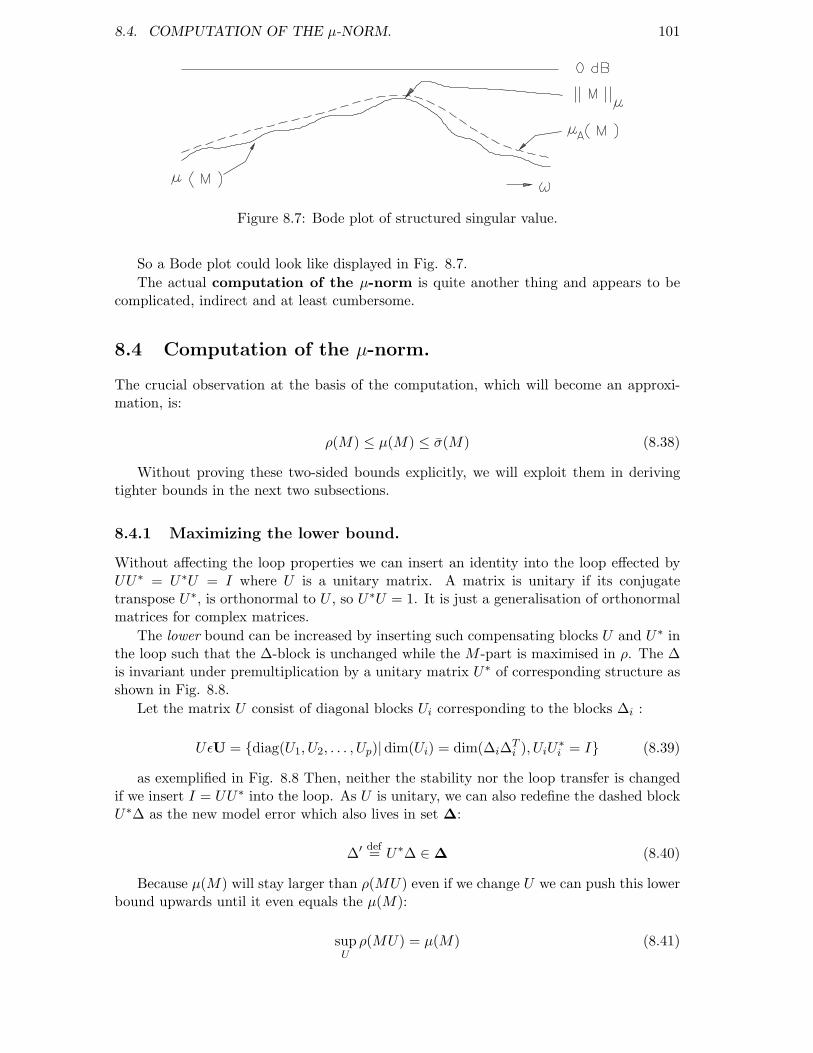
8.4. COMPUTATION OF THE µ-NORM. 101
Figure 8.7: Bode plot of structured singular value.
So a Bode plot could look like displayed in Fig. 8.7.The actual computation of the µ-norm is quite another thing and appears to be
complicated, indirect and at least cumbersome.
8.4 Computation of the µ-norm.
The crucial observation at the basis of the computation, which will become an approxi-mation, is:
ρ(M) ≤ µ(M) ≤ σ(M) (8.38)
Without proving these two-sided bounds explicitly, we will exploit them in derivingtighter bounds in the next two subsections.
8.4.1 Maximizing the lower bound.
Without affecting the loop properties we can insert an identity into the loop effected byUU∗ = U∗U = I where U is a unitary matrix. A matrix is unitary if its conjugatetranspose U∗, is orthonormal to U , so U∗U = 1. It is just a generalisation of orthonormalmatrices for complex matrices.
The lower bound can be increased by inserting such compensating blocks U and U∗ inthe loop such that the ∆-block is unchanged while the M -part is maximised in ρ. The ∆is invariant under premultiplication by a unitary matrix U∗ of corresponding structure asshown in Fig. 8.8.
Let the matrix U consist of diagonal blocks Ui corresponding to the blocks ∆i :
UεU = diag(U1, U2, . . . , Up)|dim(Ui) = dim(∆i∆Ti ), UiU
∗i = I (8.39)
as exemplified in Fig. 8.8 Then, neither the stability nor the loop transfer is changedif we insert I = UU∗ into the loop. As U is unitary, we can also redefine the dashed blockU∗∆ as the new model error which also lives in set ∆:
∆′ def= U∗∆ ∈∆ (8.40)
Because µ(M) will stay larger than ρ(MU) even if we change U we can push this lowerbound upwards until it even equals the µ(M):
supUρ(MU) = µ(M) (8.41)
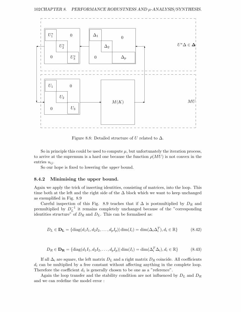
102CHAPTER 8. PERFORMANCE ROBUSTNESS AND µ-ANALYSIS/SYNTHESIS.
M(K)
∆1
∆2
∆p
0
0
U∗1
U∗2
U∗3
U1
U2
U3
U∗∆ ∈∆
MU
0
0
0
0
Figure 8.8: Detailed structure of U related to ∆.
So in principle this could be used to compute µ, but unfortunately the iteration process,to arrive at the supremum is a hard one because the function ρ(MU) is not convex in theentries uij .
So our hope is fixed to lowering the upper bound.
8.4.2 Minimising the upper bound.
Again we apply the trick of inserting identities, consisting of matrices, into the loop. Thistime both at the left and the right side of the ∆ block which we want to keep unchangedas exemplified in Fig. 8.9
Careful inspection of this Fig. 8.9 teaches that if ∆ is postmultiplied by DR andpremultiplied by D−1
L it remains completely unchanged because of the ”correspondingidentities structure” of DR and DL. This can be formalised as:
DL ∈ DL = diag(d1I1, d2I2, . . . , dpIp)|dim(Ii) = dim(∆i∆Ti ), di ∈ R (8.42)
DR ∈ DR = diag(d1I1, d2I2, . . . , dpIp)|dim(Ii) = dim(∆Ti ∆i), di ∈ R (8.43)
If all ∆i are square, the left matrix DL and a right matrix DR coincide. All coefficientsdi can be multiplied by a free constant without affecting anything in the complete loop.Therefore the coefficient d1 is generally chosen to be one as a ”reference”.
Again the loop transfer and the stability condition are not influenced by DL and DR
and we can redefine the model error :
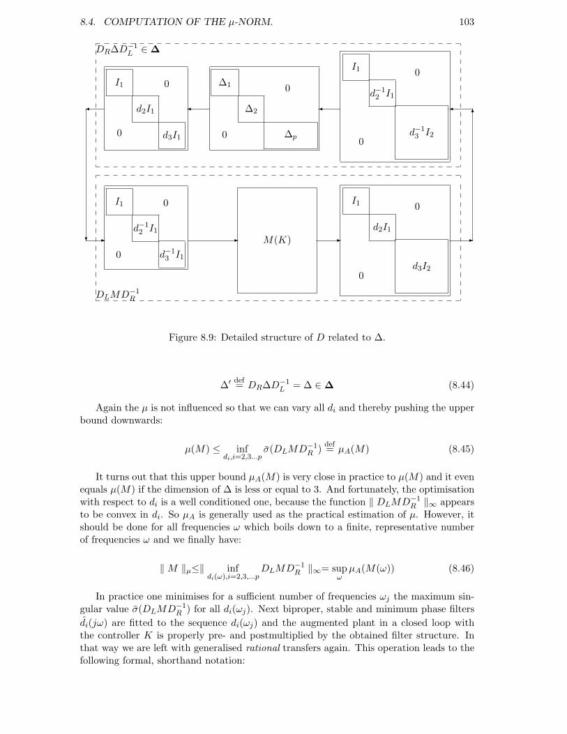
8.4. COMPUTATION OF THE µ-NORM. 103
M(K)
I1
d2I1
d3I2
0
0
I1
d−12 I1
d−13 I2
0
0
∆1
∆2
∆p
0
0
I1
d2I1
d3I1
I1
d−12 I1
d−13 I1
DR∆D−1L ∈∆
DLMD−1R
0
0
0
0
Figure 8.9: Detailed structure of D related to ∆.
∆′ def= DR∆D−1L = ∆ ∈∆ (8.44)
Again the µ is not influenced so that we can vary all di and thereby pushing the upperbound downwards:
µ(M) ≤ infdi,i=2,3...p
σ(DLMD−1R ) def= µA(M) (8.45)
It turns out that this upper bound µA(M) is very close in practice to µ(M) and it evenequals µ(M) if the dimension of ∆ is less or equal to 3. And fortunately, the optimisationwith respect to di is a well conditioned one, because the function ‖ DLMD−1
R ‖∞ appearsto be convex in di. So µA is generally used as the practical estimation of µ. However, itshould be done for all frequencies ω which boils down to a finite, representative numberof frequencies ω and we finally have:
‖M ‖µ≤‖ infdi(ω),i=2,3,...p
DLMD−1R ‖∞= sup
ωµA(M(ω)) (8.46)
In practice one minimises for a sufficient number of frequencies ωj the maximum sin-gular value σ(DLMD−1
R ) for all di(ωj). Next biproper, stable and minimum phase filtersdi(jω) are fitted to the sequence di(ωj) and the augmented plant in a closed loop withthe controller K is properly pre- and postmultiplied by the obtained filter structure. Inthat way we are left with generalised rational transfers again. This operation leads to thefollowing formal, shorthand notation:
104CHAPTER 8. PERFORMANCE ROBUSTNESS AND µ-ANALYSIS/SYNTHESIS.
‖ infdi(ω),i=2,3,...p
DLMD−1R ‖∞≈‖ DLM(K)D−1
R ‖∞ −→ infD‖ DM(K)D−1 ‖∞ (8.47)
where the distinction between DL and DR is left out of the notation as they arelinked in di anyhow. Also their rational filter structure is not explicitly indicated. As aconsequence we can write:
‖M ‖µ≈ infD‖ DMD−1 ‖∞≈ sup
ωµA(M(ω)) (8.48)
Consequently, if µA remains below 1 for all frequencies, robust stability is guaranteedand the smaller it is, the more robustly stable the closed loop system is. This finishes theµ-analysis part: given a particular controller K the µ-analysis tells you about robustnessin stability and performance.
8.5 µ-analysis/synthesis
By equation (8.46) we have a tool to verify robustness of the total augmented plant ina closed loop with controller K. The augmented plant includes both the model error-block and the artificial, fancy performance block. Consequently robust stability shouldbe understood here as concerning the generalised stability which implies that also theperformance is robust against the plant perturbations. But this is only the analysis, givena particular controlled block M which is still a function (LFT) of the controller K. Forthe synthesis of the controller we were used to minimise the H∞-norm:
infKstabilising
‖M(K) ‖∞ (8.49)
but we have just found that this is conservative and that we should minimise:
infKstabilising
‖ DM(K)D−1 ‖∞ (8.50)
However, for each new K the subsequently altered M(K) involves a new minimisation forD so that we have to solve:
infKstabilising
infD‖ DM(K)D−1 ‖∞ (8.51)
In practice this is tried to be solved by the following iteration procedure under the nameD-K-iteration process:
1. Put D = I
2. K-iteration. Compute optimal K for the last D.
3. D-iteration. Compute optimal D for the last K.
4. Has the criterion ‖ DM(K)D−1 ‖∞ changed significantly during the last two steps?If yes: goto K-iteration, if no: stop.
In practice this iteration process appears to converge usually in not too many steps. Butthere can be exceptions and in principle there is a possibility that it does not converge atall.
This formally completes the very brief introduction into µ-analysis/synthesis. A fewextra remarks will be added before a simple example will illustrate the theory.
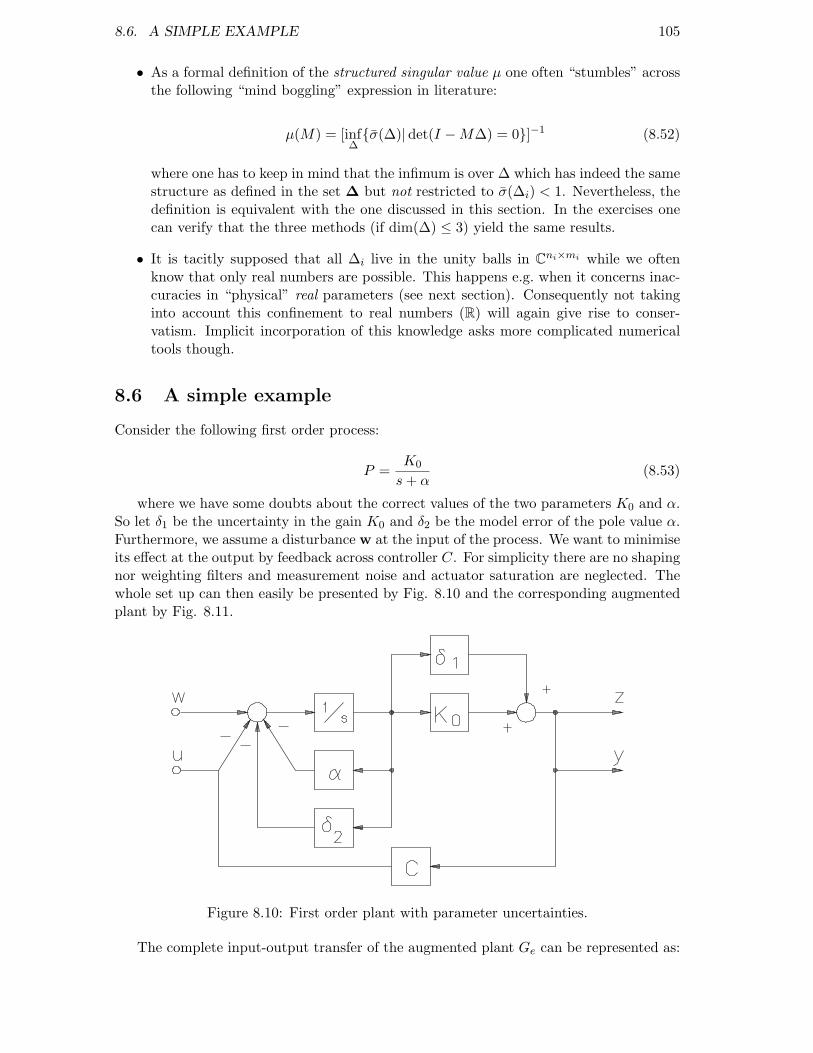
8.6. A SIMPLE EXAMPLE 105
• As a formal definition of the structured singular value µ one often “stumbles” acrossthe following “mind boggling” expression in literature:
µ(M) = [inf∆σ(∆)|det(I −M∆) = 0]−1 (8.52)
where one has to keep in mind that the infimum is over ∆ which has indeed the samestructure as defined in the set ∆ but not restricted to σ(∆i) < 1. Nevertheless, thedefinition is equivalent with the one discussed in this section. In the exercises onecan verify that the three methods (if dim(∆) ≤ 3) yield the same results.
• It is tacitly supposed that all ∆i live in the unity balls in Cni×mi while we oftenknow that only real numbers are possible. This happens e.g. when it concerns inac-curacies in “physical” real parameters (see next section). Consequently not takinginto account this confinement to real numbers (R) will again give rise to conser-vatism. Implicit incorporation of this knowledge asks more complicated numericaltools though.
8.6 A simple example
Consider the following first order process:
P =K0
s+ α(8.53)
where we have some doubts about the correct values of the two parameters K0 and α.So let δ1 be the uncertainty in the gain K0 and δ2 be the model error of the pole value α.Furthermore, we assume a disturbance w at the input of the process. We want to minimiseits effect at the output by feedback across controller C. For simplicity there are no shapingnor weighting filters and measurement noise and actuator saturation are neglected. Thewhole set up can then easily be presented by Fig. 8.10 and the corresponding augmentedplant by Fig. 8.11.
Figure 8.10: First order plant with parameter uncertainties.
The complete input-output transfer of the augmented plant Ge can be represented as:
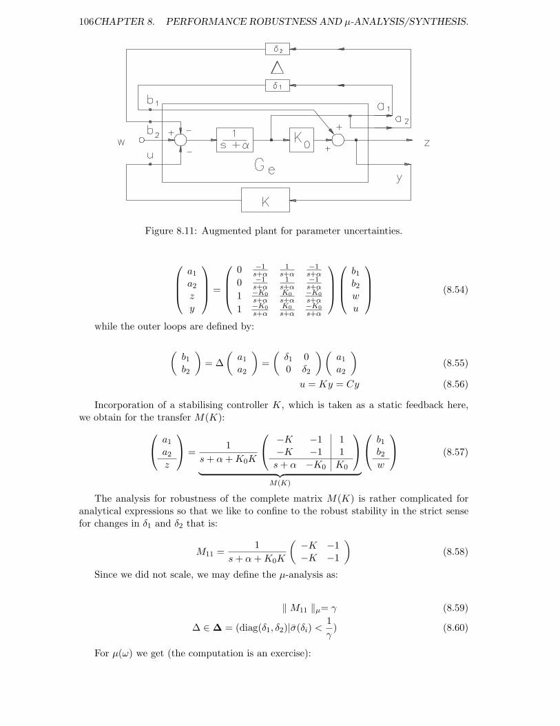
106CHAPTER 8. PERFORMANCE ROBUSTNESS AND µ-ANALYSIS/SYNTHESIS.
Figure 8.11: Augmented plant for parameter uncertainties.
a1a2zy
=
0 −1
s+α1
s+α−1s+α
0 −1s+α
1s+α
−1s+α
1 −K0s+α
K0s+α
−K0s+α
1 −K0s+α
K0s+α
−K0s+α
b1b2wu
(8.54)
while the outer loops are defined by:
(b1b2
)= ∆
(a1a2
)=(δ1 00 δ2
)(a1a2
)(8.55)
u = Ky = Cy (8.56)
Incorporation of a stabilising controller K, which is taken as a static feedback here,we obtain for the transfer M(K): a1
a2
z
=1
s+ α+K0K
−K −1 1−K −1 1s+ α −K0 K0
︸ ︷︷ ︸
M(K)
b1b2w
(8.57)
The analysis for robustness of the complete matrix M(K) is rather complicated foranalytical expressions so that we like to confine to the robust stability in the strict sensefor changes in δ1 and δ2 that is:
M11 =1
s+ α+K0K
( −K −1−K −1
)(8.58)
Since we did not scale, we may define the µ-analysis as:
‖M11 ‖µ= γ (8.59)
∆ ∈∆ = (diag(δ1, δ2)|σ(δi) <1γ
) (8.60)
For µ(ω) we get (the computation is an exercise):
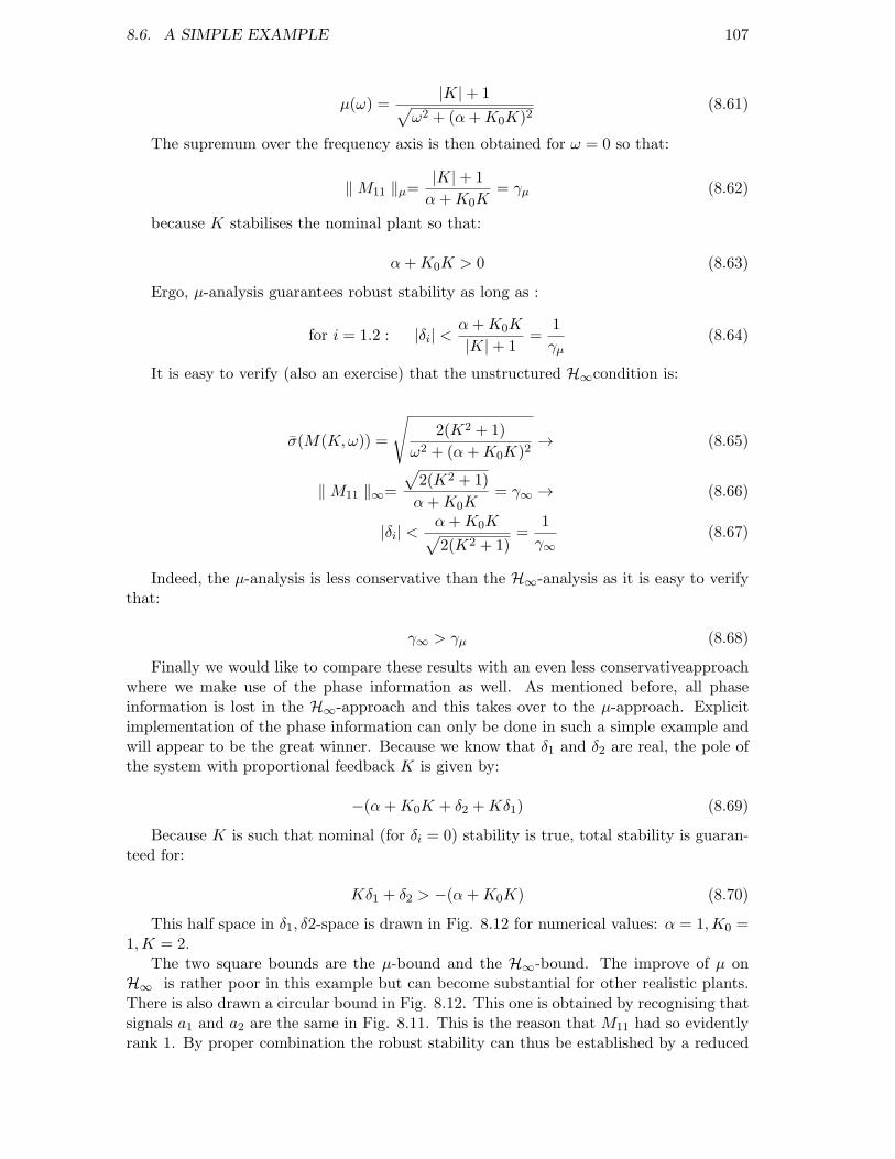
8.6. A SIMPLE EXAMPLE 107
µ(ω) =|K|+ 1√
ω2 + (α+K0K)2(8.61)
The supremum over the frequency axis is then obtained for ω = 0 so that:
‖M11 ‖µ=|K|+ 1α+K0K
= γµ (8.62)
because K stabilises the nominal plant so that:
α+K0K > 0 (8.63)
Ergo, µ-analysis guarantees robust stability as long as :
for i = 1.2 : |δi| < α+K0K
|K|+ 1=
1γµ
(8.64)
It is easy to verify (also an exercise) that the unstructured H∞condition is:
σ(M(K,ω)) =
√2(K2 + 1)
ω2 + (α+K0K)2→ (8.65)
‖M11 ‖∞=
√2(K2 + 1)α+K0K
= γ∞ → (8.66)
|δi| < α+K0K√2(K2 + 1)
=1γ∞
(8.67)
Indeed, the µ-analysis is less conservative than the H∞-analysis as it is easy to verifythat:
γ∞ > γµ (8.68)
Finally we would like to compare these results with an even less conservativeapproachwhere we make use of the phase information as well. As mentioned before, all phaseinformation is lost in the H∞-approach and this takes over to the µ-approach. Explicitimplementation of the phase information can only be done in such a simple example andwill appear to be the great winner. Because we know that δ1 and δ2 are real, the pole ofthe system with proportional feedback K is given by:
−(α+K0K + δ2 +Kδ1) (8.69)
Because K is such that nominal (for δi = 0) stability is true, total stability is guaran-teed for:
Kδ1 + δ2 > −(α+K0K) (8.70)
This half space in δ1, δ2-space is drawn in Fig. 8.12 for numerical values: α = 1,K0 =1,K = 2.
The two square bounds are the µ-bound and the H∞-bound. The improve of µ onH∞ is rather poor in this example but can become substantial for other realistic plants.There is also drawn a circular bound in Fig. 8.12. This one is obtained by recognising thatsignals a1 and a2 are the same in Fig. 8.11. This is the reason that M11 had so evidentlyrank 1. By proper combination the robust stability can thus be established by a reduced
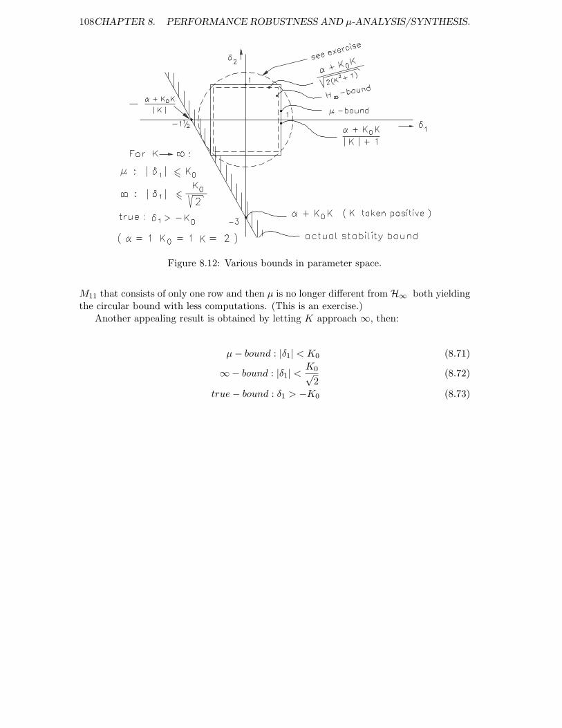
108CHAPTER 8. PERFORMANCE ROBUSTNESS AND µ-ANALYSIS/SYNTHESIS.
Figure 8.12: Various bounds in parameter space.
M11 that consists of only one row and then µ is no longer different from H∞ both yieldingthe circular bound with less computations. (This is an exercise.)
Another appealing result is obtained by letting K approach ∞, then:
µ− bound : |δ1| < K0 (8.71)
∞− bound : |δ1| < K0√2
(8.72)
true− bound : δ1 > −K0 (8.73)
8.7. EXERCISES 109
8.7 Exercises
9.1: Show that, in case M12 = 0 or M21 = 0, the robust performance condition is fulfilledif both the robust stability and the performance for the nominal model are guaranteed.Does this case, off-diagonal terms of M zero, make sense ?
9.2: Given the three examples in this chapter:
M =(
1/2 00 1/2
) (2 00 1
) (0 100 0
)(8.74)
Compute the µ-norm if ∆ =(δ1 00 δ2
)according to the second definition :
µ = [inf∆σ(∆)|det (I −M∆) = 0]−1 (8.75)
9.3: Given:
M =( −1/2 1/2−1/2 1/2
)∆ =
(δ1 00 δ2
)(8.76)
a) Compute ρ and σ of M . Are these good bounds for µ ?
b) Compute µ in three ways.
9.4: Compute explicitly ‖M11 ‖∞ and ‖M11 ‖µ for the example in this chapter where:
M11 =1
s+ α+K0K
(K −1K −1
)(8.77)
What happens if we use the fact that the the error block output signals a1 and a2 arethe same , so that ∆ can be defined as ∆ = [ δ1 δ2 ]T ? Show that the circular boundof the last Fig. 8.12 results.

110CHAPTER 8. PERFORMANCE ROBUSTNESS AND µ-ANALYSIS/SYNTHESIS.
Chapter 9
Filter Selection and Limitations.
In this chapter we will discuss several aspects of filter selection in practice. First wewill show how signal characteristics and model errors can be measured and how thesemeasurements together with performance aims can lead to effective filters. Effective inthe sense, that solutions with ‖ M ‖∞< γ ≈ 1 are feasible without contradicting e.g.”S+T=I” and other fundamental bounds.
Apart from the chosen filters there are also characteristics of the process itself, whichultimately bound the performance, for instance RHP (=Right Half Plane) zeros and/orpoles, actuator and output ranges, less inputs than outputs etc. We will shortly indicatetheir effects such that one is able to detect the reason, why γ ≈ 1 could not be obtainedand what the best remedy or compromise can be.
9.1 A zero frequency set-up.
9.1.1 Scaling
The numerical values of the various signals in a controlled system are usually expressedin their physical dimensions like m, N , V , A, o, . . . . Next, depending on the size of thesignals, we also have a rough scaling possibility in the choice of the units. For instancea distance will basically be expressed in meters, but in order to avoid very large or verysmall numbers we can choose among km, mm, µm, A or lightyears. Still this is toorough a scaling to compare signals of different physical dimensions. As a matter of factthe complete concept of mapping normed input signals onto normed output signals, asdiscussed in chapter 5, incorporates the basic idea of appropriate comparison of physicallydifferent signals by means of the input characterising filters V∗ and output weightingfilters W∗. The filter choice is actually a scaling problem for each frequency. So let usstart in a simplified context and analyse the scaling first for one particular frequency,say ω = 0. Scaling on physical, numerically comparable units as indicated above is notaccurate enough and a trivial solution is simply the familiar technique of eliminatingphysical dimensions by dividing by the maximum amplitude. So each signal s can thenbe expressed in dimensionless units as s according to:
s = 1smax
s = Wss s = smaxs = Vss smax = sup(|s|) (9.1)
where supremum should be read as the extreme value it can take given the corre-sponding (expected) range. For a typical SISO-plant configuration such scaling leads tothe blockscheme of Fig. 9.1.
111
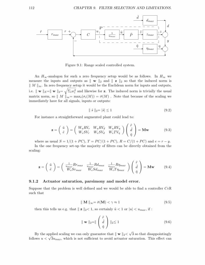
112 CHAPTER 9. FILTER SELECTION AND LIMITATIONS.
rmax C1
umax P zmax
dmax
ηmax
P
r r +
−
u u z z
d
η
y
d
η
Figure 9.1: Range scaled controlled system.
An H∞-analogon for such a zero frequency setup would be as follows. In H∞ wemeasure the inputs and outputs as ‖ w ‖2 and ‖ z ‖2 so that the induced norm is‖M ‖∞. In zero frequency setup it would be the Euclidean norm for inputs and outputs,
i.e. ‖ w ‖E=‖ w ‖2=√
Σiw2i and likewise for z. The induced norm is trivially the usual
matrix norm, so ‖ M ‖∞= maxi(σi(M)) = σ(M) . Note that because of the scaling weimmediately have for all signals, inputs or outputs:
‖ s ‖2= |s| ≤ 1 (9.2)
For instance a straightforward augmented plant could lead to:
z =(ue
)=(WuRVr WuRVd WuRVη
WeSVr WeSVd WeTVη
) r
dη
= Mw (9.3)
where as usual S = 1/(1 + PC), T = PC/(1 + PC), R = C/(1 + PC) and e = r − y.In the one frequency set-up the majority of filters can be directly obtained from the
scaling:
z =(ue
)=( 1
umaxRrmax
1umax
Rdmax1
umaxRηmax
WeSrmax WeSdmax WeTηmax
) r
dη
= Mw (9.4)
9.1.2 Actuator saturation, parsimony and model error.
Suppose that the problem is well defined and we would be able to find a controller CεRsuch that
‖M ‖∞= σ(M) < γ ≈ 1 (9.5)
then this tells us e.g. that ‖ z ‖2< 1, so certainly u < 1 or |u| < umax, if :
‖ w ‖2=‖ r
dη
‖2≤ 1 (9.6)
By the applied scaling we can only guarantee that ‖ w ‖2<√
3 so that disappointinglyfollows u <
√3umax, which is not sufficient to avoid actuator saturation. This effect can
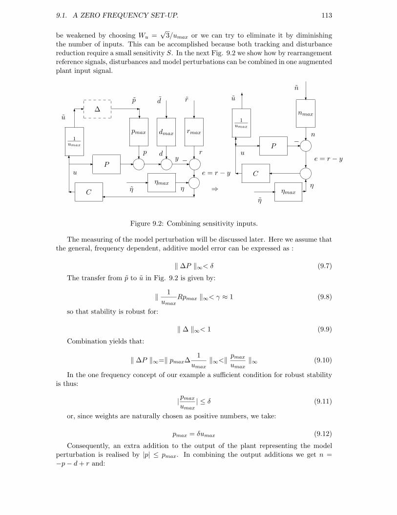
9.1. A ZERO FREQUENCY SET-UP. 113
be weakened by choosing Wu =√
3/umax or we can try to eliminate it by diminishingthe number of inputs. This can be accomplished because both tracking and disturbancereduction require a small sensitivity S. In the next Fig. 9.2 we show how by rearrangementreference signals, disturbances and model perturbations can be combined in one augmentedplant input signal.
C
1umax
P
pmax dmax rmax
C
1umax
P
nmax
ηmax
∆
ηmax
−
u
u
p d r
η η
y
e = r − y
⇒
p d r
u
n
n
e = r − y
η
η
u
−
Figure 9.2: Combining sensitivity inputs.
The measuring of the model perturbation will be discussed later. Here we assume thatthe general, frequency dependent, additive model error can be expressed as :
‖ ∆P ‖∞< δ (9.7)
The transfer from p to u in Fig. 9.2 is given by:
‖ 1umax
Rpmax ‖∞< γ ≈ 1 (9.8)
so that stability is robust for:
‖ ∆ ‖∞< 1 (9.9)
Combination yields that:
‖ ∆P ‖∞=‖ pmax∆1
umax‖∞<‖ pmax
umax‖∞ (9.10)
In the one frequency concept of our example a sufficient condition for robust stabilityis thus:
|pmax
umax| ≤ δ (9.11)
or, since weights are naturally chosen as positive numbers, we take:
pmax = δumax (9.12)
Consequently, an extra addition to the output of the plant representing the modelperturbation is realised by |p| ≤ pmax. In combining the output additions we get n =−p− d+ r and:
114 CHAPTER 9. FILTER SELECTION AND LIMITATIONS.
nmax = pmax + dmax + rmax (9.13)
Note that the sign of p and d, actually being a phase angle, does not influence theweighting. Also convince yourself of the substantial difference of diminishing the numberof inputs compared with increasing the Wu with a factor
√3. We have |n| ≤ 1 contrary
to the original three inputs |p| ≤ 1, |d| ≤ 1 and |r| ≤ 1, implying a reduction of a factor3 in stead of
√3. The 2-norm applied to w in the two blockschemes of Fig. 9.2 would
indeed yield the factor√
3 as√‖ p ‖2 + ‖ d ‖2 + ‖ r ‖2 ≤ √3 contrary to
√‖ n ‖2 ≤ 1.By reducing the number of inputs we have done so taking care that the maximum valuewas retained. If several 2-normed signals are placed in a vector, the total 2-norm takesthe average of the energy or power. Consequently we are confronted again with the factthat not H∞ is suited for protection against actuator saturation, but l1-control is.
Note, that for the proper quantisation of the actuator input signal we had to actuallyadd the reference signal, the disturbance and the model error output. For robust stabilityalone it is now sufficient that:
nmax = δumax (9.14)
whatever the derivation of nmax might be. In the next section we will see that in thefrequency dependent case, a real prevention of actuator saturation can never be guaranteedin H∞-control. Actual practice will then be to combine Vd and Vr into Vn, heuristicallydefine a Wu and verify whether for robust stability the condition:
∀ω : |VnWu| ≤ δ(ω) (9.15)
is fulfilled. If not, either Vn or Wu should be corrected.
9.1.3 Bounds for tracking and disturbance reduction.
Till sofar we have discussed all weights except for the error weight We. Certainly wewould like to choose We as big and broad as possible in order to keep the error e as smallas possible. If we forget about the measurement noise η for the moment and apply thesimplified right scheme of Fig. 9.2, we obtain a simple mixed sensitivity problem:(
ue
)=( 1
umax
C1+PCnmax
We1
1+PCnmax
)(n) =
(m11m21
)(n) (9.16)
Because σ(M) =√m2
11 +m221 we can easily compute the optimal controller, that
minimises σ(M), as:
C = W 2e Pu
2max (9.17)
In order to keep σ(M) ≈ 1 to prevent actuator saturation we can put σ(M) = 1 forthe computed controller C yielding:
We = 1/√n2
max − P 2u2max (9.18)
A special case occurs for |Pumax| = |nmax| which simply states that the range ofthe actuator is exactly sufficient to cause the output z of plant P to compensate for the”disturbance” n. So if actuator range and plant gain is sufficiently large we can chooseWe =∞ and thus C =∞ so that M becomes:
9.1. A ZERO FREQUENCY SET-UP. 115
M =( nmax
Pumax
0
)(9.19)
and no error results while σ(M) = |m11| = 1.If |Pumax| > |nmax|, their is plenty of choice for the controller and the H∞ criterion is
minimised by decreasing |m11| more at the cost of a small increase of |m21|. Note that thiscontrol design is different from minimising |m21| under the constraint of |m11| ≤ 1. Forthis simple example the last problem can be solved, but the reader is invited to do thisand by doing so to obtain an impression of the tremendous task for a realistically sizedproblem.
If |Pumax| < |nmax|, it is principally impossible to compensate all ”possible distur-bance” n. This is reflected in the maximal weight We we can choose that allows for aσ(M) ≈ 1. Some algebra shows that:
1Wenmax
=
√1− P 2u2
max
n2max
(9.20)
If e.g. only half the n can be compensated, i.e. |Pumax| = 12 |nmax|, we have |S| ≈
1Wenmax
=√
34 which is very poor. This represents the impossibility to track better than
50% or reduce the disturbance more than 50%. If one increases the weight We one isconfronted with a similar increase of γ and no solution ‖M ‖∞≈ 1 can be obtained. Onecan test this beforehand by analysing the scaled plant as indicated in Fig. 9.1. The plantP has been normalised internally according to:
P = zmaxP1
umax(9.21)
so that P is the transfer from u, maximally excited actuator normalised on 1, tomaximal, undisturbed, scaled output z. Suppose now that |P | < 1. It tells you that notall outputs in the intended output range can be obtained due to the actual actuator. Themaximal input umax can only yield:
|z| = |zmaxP1
umaxumax| = |zmaxP | < zmax (9.22)
Consequently, if we have obviously rmax ≈ zmax for a tracking system, the trackingerror e = r − y can never become small.
For SISO plants this effect is quite obvious, but for MIMO systems the same internalscaling of plant P can be very revealing in detecting these kind of internal insufficienciesas we will show later.
On the other hand, if the gain of the scaled plant P is larger than 1, one should notthink that the way is free to zero sensitivity S. For real systems, where the full frequencydependence plays a role, we will see plenty of limiting effects. Only for ω = 0 we are usedto claim zero sensitivity in case of integrator(s) in the loop. In that case we have indeedinfinite gain (1/(jω)) similar to the previous example by taking C = ∞. Nevertheless inpractice we always have to deal with the sensor and inevitable sensor noise η. If we indeedhave S = 0, inevitably T = 1 and e = Tη = η. So in its full extent the measurementnoise is present in the error, which simply reflects the trivial fact that you can never trackbetter than the accuracy of the sensor. So sensor noise bounds both traking error anddisturbance rejection and should be brought in properly by the weight ηmax in our examplein order to minimise its effect in balance with the other bounds and claims.
116 CHAPTER 9. FILTER SELECTION AND LIMITATIONS.
9.2 Frequency dependent weights.
9.2.1 Weight selection by scaling per frequency.
In the previous section the single frequency case served as a very simple concept to illus-trate some fundamental limitations, that certainly exist in the full, frequency dependentsituation. All effects take over, where we have to consider a similar kind of scaling butactually for each frequency. Usually the H∞-norm is presented as the induced norm ofthe mapping from the L2 space to the L2 space. In engineering terms we then talk aboutthe (square-root of) the energy of inputs ‖ w ‖2 towards the (square-root of) the energy ofoutputs ‖ z ‖2. Mathematically, this is fine, but in practice we seldomly deal with finite en-ergy signals. Fortunately, the H∞-norm is also the induced norm for mapping powers ontopowers or even expected powers onto expected powers as explained in chapter 5. If oneconsiders a signal to be deterministic, where certain characteristics may vary, the powercan simply be obtained by describing that signal by a Fourier series, where the Fouriercoefficients directly represent the maximal amplitude per frequency. This maximum canthus be used as a scaling for each frequency analogous to the one frequency example ofthe previous section. On the other hand if one considers the signal to be stochastic (sta-tionary, one sample from an ergodic ensemble), one can determine the power density Φs
and use the square-root of it as the scaling. One can even combine the two approaches,for instance stochastic disturbances and deterministic reference signals. In that case oneshould bear in mind that the dimensions are fundamentally different and a proper con-stant should be brought in for appropriate weighting. Only if one sticks to one kind ofapproach, any scaling constant c is irrelevant as it disappears by the fundamental divisionin the definition:
‖M ‖∞= supw
‖Mw ‖power
‖ w ‖power= sup
w
‖ cMw ‖power
‖ cw ‖power(9.23)
Furthermore, as we have learned from the ω = 0 scaling, the maxima (=range) ofthe inputs scale and thus define the input characterising filters directly, while the outputfilters are determined by the inverse so that we obtain e.g. for input v to output x:
WxMxvVv =1
xmaxMxvvmax =
1cxmax
Mxvcvmax (9.24)
So again the constant is irrelevant, unless input- and outputfilters are defined withdifferent constants. In chapter 5 it has been illustrated how the constant relating thedeterministic power contents to a power density value can be obtained. It has been doneby explicitely computing the norms in both concepts for an example signal set that canserve for both interpretations. From here on we suppose that one has chosen the oneor other convention and that we can continue with a scaling per frequency similar tothe scaling in the previous section. So smax(ω) represents the square-root of any power-definition for signal s(jω), e.g. smax(ω) =
√Φss(jω). Remember that the phase of filters
and thus of smax(ω) is irrelevant. Straightforward implementation of scaling would thenlead to:
s(ω) = 1smax(ω)s(ω)→Ws(jω)s(ω) s(ω) = smax(ω)s(ω)→ Vs(jω)s(ω) (9.25)
Arrows have been used in above equations because immediate choice of e.g.Vs(jω) =smax(ω) =
√Φss(jω) would unfortunately rarely yield a rational transferfunction Vs(jω)

9.2. FREQUENCY DEPENDENT WEIGHTS. 117
and all available techniques and algorithms in H∞ design are only applicable for rationalweights. Therefore one has to come up with not too complicated rational weights Vs orWs satisfying:
|Vs(jω)| ≥ |smax(ω)| e.g.= |
√Φss(jω)| |Ws(jω)| ≥ | 1
smax(ω)| e.g.
= |√
Φss(jω)| (9.26)
The routine ”magshape” in Matlab-toolbox LMI can help you with this task. Thereyou can define a number of points in the Bode amplitude plot where the routine providesyou with a low order rational weight function passing through these points. When youhave a series of measured or computed weights in frequency domain, you can easily comeup with a rational weight sufficiently close (from above) to them.
Whether you use these routines or you do it by hand, you have watch the followingside conditions:
1. The weighting filter should be stable and minimum phase. Be sure that there are noRHP (=Right Half Plane) poles or zeros. Unstable poles would disrupt the conditionof stability for the total design, also for the augmented plant. Nonminimum phasezeros would prohibit implicit inversion of the filters in the controller design.
2. Poles or zeros on the imaginary axis cause numerical problems for virtually the samereason and should thus be avoided. If one wants an integral weighting, i.e. a polein the origin, in order to obtain an infinite weight at frequency zero and to forcethe design to place an integrator in the controller, one should approximate this inthe filter. In practice it means that one positions a pole in the weight very closeto the origin in the LHP (Left Half Plane). The distance to the origin should bevery small compared to the distances of other poles and zeros in plant and filters.Alternatively, one could properly include an integrator to the plant and separate itout to the controller lateron, when the design is finished. In that case be thoughtfulabout how the integrator is included in the plant (not just concatenation!).
3. The filters should be preferably be biproper. Any pole zero excess would in fact causezeros at infinity, that make the filter uninvertable and inversion happens implicitlyin the controller design.
4. The dynamics of the generalised plant should not exceed about 5 decades on thefrequency scale for numerical reasons dependent on the length of the mantissa inyour computer. So double precision can increase the number of decades. In singleprecision it thus means that the smallest radius (=distance to the origin) divided bythe largest radius of all poles and zeros of plant and filters should not be less than10−5.
5. The filters are preferably of low order. Not only the controller will be simpler asit will have the total order of the augmented plant. Also filters very steep at theborder of the aimed tracking band will cause problems for the robustness as smalldeviations will easily let the fast loops in Nyquist plot tresspass the hazardous point-1.
9.2.2 Actuator saturation: Wu
The characterisation or weighting filters of most signals can sufficiently well be obtainedas described in the previous subsection. A characterisation per frequency is well in line
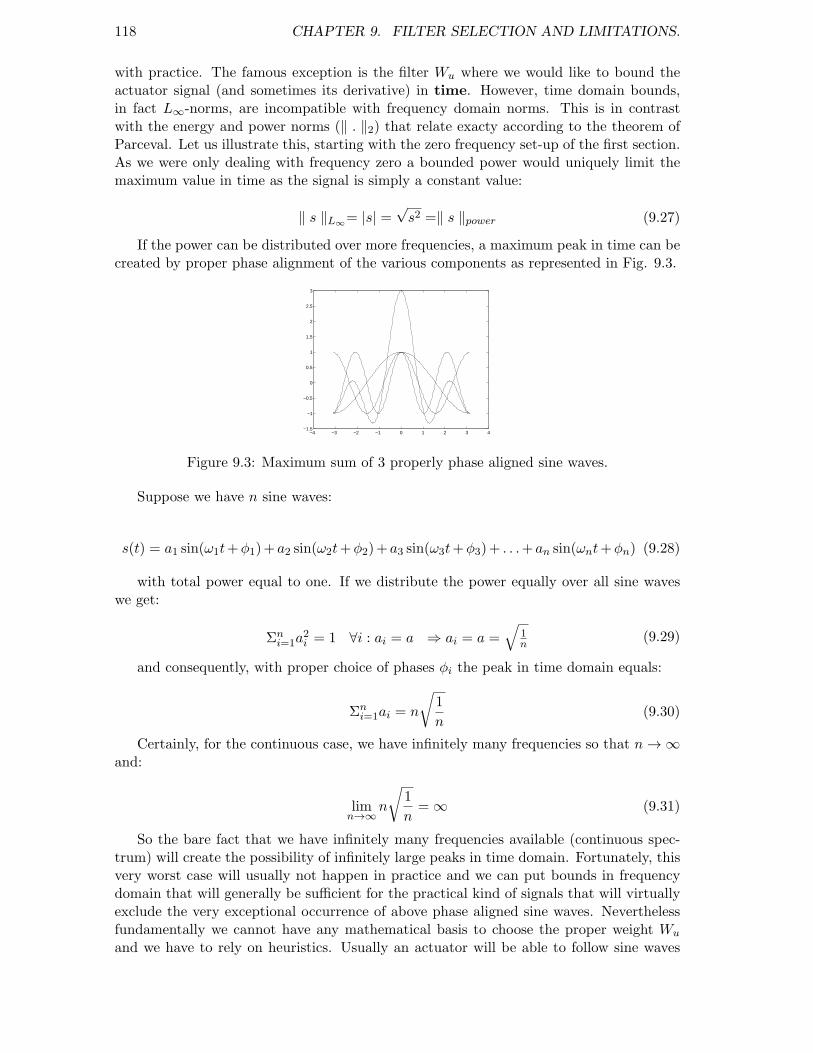
118 CHAPTER 9. FILTER SELECTION AND LIMITATIONS.
with practice. The famous exception is the filter Wu where we would like to bound theactuator signal (and sometimes its derivative) in time. However, time domain bounds,in fact L∞-norms, are incompatible with frequency domain norms. This is in contrastwith the energy and power norms (‖ . ‖2) that relate exacty according to the theorem ofParceval. Let us illustrate this, starting with the zero frequency set-up of the first section.As we were only dealing with frequency zero a bounded power would uniquely limit themaximum value in time as the signal is simply a constant value:
‖ s ‖L∞= |s| =√s2 =‖ s ‖power (9.27)
If the power can be distributed over more frequencies, a maximum peak in time can becreated by proper phase alignment of the various components as represented in Fig. 9.3.
−4 −3 −2 −1 0 1 2 3 4−1.5
−1
−0.5
0
0.5
1
1.5
2
2.5
3
Figure 9.3: Maximum sum of 3 properly phase aligned sine waves.
Suppose we have n sine waves:
s(t) = a1 sin(ω1t+φ1)+a2 sin(ω2t+φ2)+a3 sin(ω3t+φ3)+ . . .+an sin(ωnt+φn) (9.28)
with total power equal to one. If we distribute the power equally over all sine waveswe get:
Σni=1a
2i = 1 ∀i : ai = a ⇒ ai = a =
√1n
(9.29)
and consequently, with proper choice of phases φi the peak in time domain equals:
Σni=1ai = n
√1n
(9.30)
Certainly, for the continuous case, we have infinitely many frequencies so that n→∞and:
limn→∞n
√1n
=∞ (9.31)
So the bare fact that we have infinitely many frequencies available (continuous spec-trum) will create the possibility of infinitely large peaks in time domain. Fortunately, thisvery worst case will usually not happen in practice and we can put bounds in frequencydomain that will generally be sufficient for the practical kind of signals that will virtuallyexclude the very exceptional occurrence of above phase aligned sine waves. Neverthelessfundamentally we cannot have any mathematical basis to choose the proper weight Wu
and we have to rely on heuristics. Usually an actuator will be able to follow sine waves
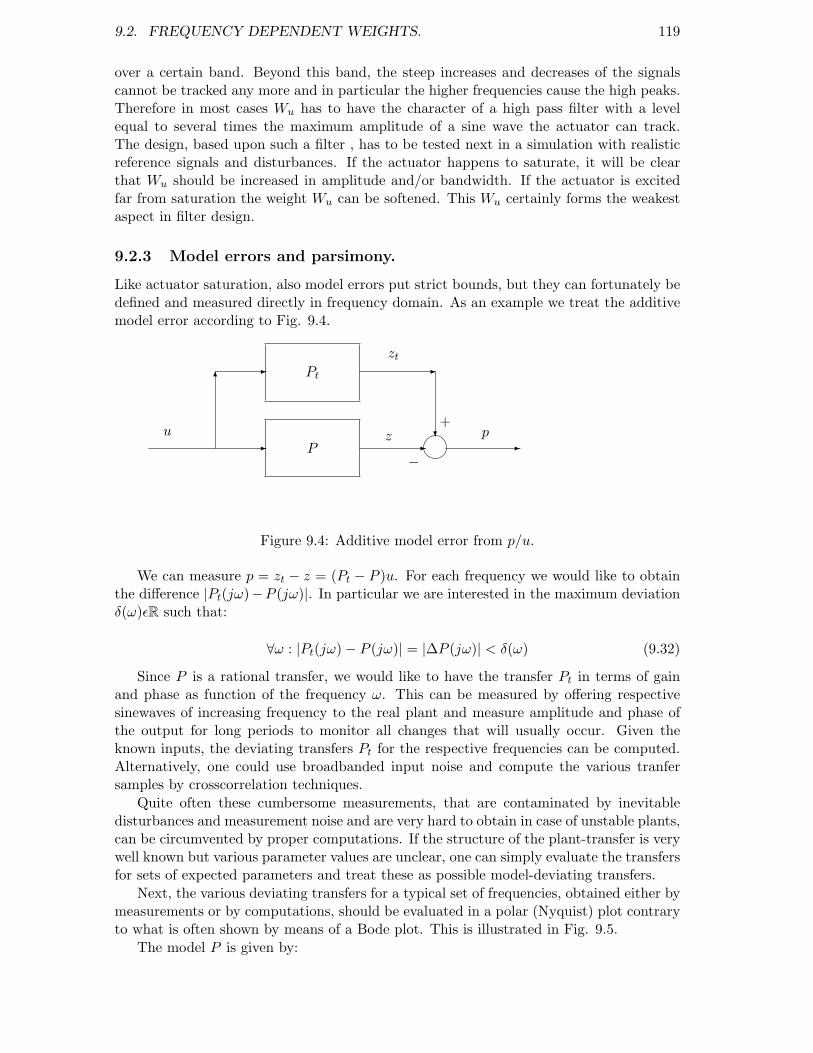
9.2. FREQUENCY DEPENDENT WEIGHTS. 119
over a certain band. Beyond this band, the steep increases and decreases of the signalscannot be tracked any more and in particular the higher frequencies cause the high peaks.Therefore in most cases Wu has to have the character of a high pass filter with a levelequal to several times the maximum amplitude of a sine wave the actuator can track.The design, based upon such a filter , has to be tested next in a simulation with realisticreference signals and disturbances. If the actuator happens to saturate, it will be clearthat Wu should be increased in amplitude and/or bandwidth. If the actuator is excitedfar from saturation the weight Wu can be softened. This Wu certainly forms the weakestaspect in filter design.
9.2.3 Model errors and parsimony.
Like actuator saturation, also model errors put strict bounds, but they can fortunately bedefined and measured directly in frequency domain. As an example we treat the additivemodel error according to Fig. 9.4.
P
Pt
u
zt
z p+
−
Figure 9.4: Additive model error from p/u.
We can measure p = zt − z = (Pt − P )u. For each frequency we would like to obtainthe difference |Pt(jω)−P (jω)|. In particular we are interested in the maximum deviationδ(ω)εR such that:
∀ω : |Pt(jω)− P (jω)| = |∆P (jω)| < δ(ω) (9.32)
Since P is a rational transfer, we would like to have the transfer Pt in terms of gainand phase as function of the frequency ω. This can be measured by offering respectivesinewaves of increasing frequency to the real plant and measure amplitude and phase ofthe output for long periods to monitor all changes that will usually occur. Given theknown inputs, the deviating transfers Pt for the respective frequencies can be computed.Alternatively, one could use broadbanded input noise and compute the various tranfersamples by crosscorrelation techniques.
Quite often these cumbersome measurements, that are contaminated by inevitabledisturbances and measurement noise and are very hard to obtain in case of unstable plants,can be circumvented by proper computations. If the structure of the plant-transfer is verywell known but various parameter values are unclear, one can simply evaluate the transfersfor sets of expected parameters and treat these as possible model-deviating transfers.
Next, the various deviating transfers for a typical set of frequencies, obtained either bymeasurements or by computations, should be evaluated in a polar (Nyquist) plot contraryto what is often shown by means of a Bode plot. This is illustrated in Fig. 9.5.
The model P is given by:
120 CHAPTER 9. FILTER SELECTION AND LIMITATIONS.
10−1
100
101
−30
−20
−10
0
10
Frequency (rad/sec)
Gai
n dB
10−1
100
101
−30
−60
−90
0
Frequency (rad/sec)
Pha
se d
eg
0 0.5 1 1.5
−0.6
−0.4
−0.2
0
0.2
0.4
0.6
Real Axis
Imag
Axi
s
MX
X
X
X
Figure 9.5: Additive model errors in Bode and Nyquist plots.
P =1
s+ 1(9.33)
while deviating transfers Pt are taken as:
Pt = .8s+.8 or 1.2
s+1.2 or .8s+1.2 or 1.2
s+.8 (9.34)
Given the Bode plot one is tended to take the width of the band in the gain plot as ameasure for the additive model error for each frequency. This would lead to:
maxPt
||Pt| − |P || (9.35)
which is certainly wrong. In the Nyquist plot we have indicated for ω = 1 the modeltransfer by ’M’ and the several deviating transfers by ’X’. The maximum model error isclearly given by the radius of the smallest circle around ’M’ that encompasses all plants’X’. Then we really obtain the vectorial differences for each ω:
δ(ω) = maxPt
|Pt(jω)− P (jω)| (9.36)
The reader is invited to analyse how the wrong measure of equation 9.35 can bedistinguished in the Nyquistplot.
Finally we have the following bounds for each frequency:
|∆P (jω)| < δ(ω) (9.37)
The signal p in Fig. 9.4 is that component in the disturbance free output of thetrue proces Pt due to input u, that is not accounted for by the model output Pu. Thiscomponent can be represented by an extra disturbance at the output in the generalisedplant like in Fig. 9.2, but now with a weighting filter p = Vp(jω)p. If the goal ‖M ‖∞<γ ≈ 1 we have:
‖WuRVp ‖∞< 1⇐⇒ ∀ω : |WuRVp| < 1 (9.38)
For robust stability, based on the small gain theorem, we have as condition:
9.2. FREQUENCY DEPENDENT WEIGHTS. 121
‖ R∆P ‖∞< 1⇐⇒ ∀ω : |R∆P | < 1⇐⇒ (9.39)
∀ω : |WuRVp| |∆P ||WuVp| < 1 (9.40)
Given the bounded transfer of equation 9.38, a sufficient condition is:
∀ω : |∆P | < |WuVp| (9.41)
and this can be guaranteed if the weights are sufficiently large such that the boundedmodel perturbations of equation 9.37 can be brought in as:
∀ω : |∆P | < δ(ω) < |WuVp| (9.42)
Of course, for stability also the other input weight filters Vd, Vr or even Vη in stead ofVp could have been used, because they all combined with Wu limit the control sensitivityR. Consequently, for robust stability it is sufficient to have:
∀ω : δ(ω) < sup|WuVd|, |WuVr|, |WuVη| (9.43)
If this condition is fullfilled, we don’t have to introduce an extra filter Vp for stability.The extra exogenous input p can be prefered for proper quantisation of the control signalu, but this can also be done by increasing Wu properly.
The best is to combine the exogeneous inputs d, r and p into a signal n, like we did insection 9.1.2, but now with appropriate combination for each frequency. This boils downto finding a rational filter transfer Vn(jω) such that:
∀ω : |Vn(jω)| ≥ |Vd(jω)|+ |Vr(jω)|+ |Vp(jω)| (9.44)
Again the routine ”magshape” in the LMI-toolbox can help here.Pragmatically, one usually combines only Vd and Vr into Vn and cheques whether:
∀ω : δ(ω) < |Wu(jω)Vn(jω)| (9.45)
is satisfied. If not, the weighting filter Wu is adapted until the condition is satisfied.
9.2.4 We bounded by fundamental constraint: S + T = I
For a typical low-sized H∞ problem like:
z =(ue
)=(WuRVn WuRVη
WeSVn WeTVη
)(nη
)= Mw (9.46)
all weights have been discussed except for the performance weight We. The charac-terising filters of the exogenous inputs n and η left little choice as these were determinedby the actual signals to be expected for the closed loop system. The control weightingfilter Wu was defined by rigorous bounds derived from actuator limitations and modelperturbations. Now it is to be seen how good a final performance can be obtained byoptimum choice of the errorfilter We. We would like to see that the final closed loop sys-tem shows good tracking behaviour and disturbance rejection for a broad frequency band.Unfortunately, the We will appear to be restricted by many bounds, induced by limita-tions in actuators, sensors, model accuracy and the dynamic properties of the plant to becontrolled. The influence of the plant dynamics will be discussed in the next section. Here
122 CHAPTER 9. FILTER SELECTION AND LIMITATIONS.
we will show how the influences of actuator, sensor and model accuracy put restrictionson the performance via respectively Wu, Vη and the combination of Wu, Vn and Vη.
Mentioned filters all bound the complementarity sensitivity T as a contraint:
‖WuRVn ‖∞< 1 ⇔ ∀ω : |WuRVn| = |WuP−1TVn| < 1 (9.47)
‖WuRVη ‖∞< 1 ⇔ ∀ω : |WuRVη| = |WuP−1TVη| < 1 (9.48)
‖WeTVη ‖∞< 1 ⇔ ∀ω : |WeTVη| < 1 (9.49)
In above inequalities the plant transfer P , that is not optional contrary to the controllerC, functions as part of the weights on T . Because the T is bounded accordingly thefreedom in the performance represented by the sensitivity S is bounded on the basis ofthe fundamental constraint S + T = I.
The constraints on T can be represented as ‖W2TV2 ‖∞< 1 whereW2 and V2 representthe various weight combinations of inequalities 9.47-9.49. Renaming the performance aimas:
‖WeSVn ‖∞def= ‖W1SV1 ‖∞< 1 (9.50)
Now we can repeat the comments made in section 7.5.The H∞ design problem requires:
‖W1SV1 ‖∞< 1⇔ ∀ω : |S(jω)| < |W1(jω)−1V1(jω)−1| (9.51)‖W2TV2 ‖∞< 1⇔ ∀ω : |T (jω)| < |W2(jω)−1V2(jω)−1| (9.52)
A typical weighting situation for the mixed sensitivity problem is displayed in Fig. 9.6.
Figure 9.6: Typical mixed sensitivity weights.
It is clear that not both |S| < 1/2 and |T | < 1/2 can be obtained, because S + T = 1for the SISO-case. Consequently the intersection point of the inverse weights should begreater than 1:
∃ω :1
|W1V1| =1
|W2V2| > 1/2 (9.53)
This is still too restrictive, because it is not to be expected that equal phase 0 can beaccomplished by any controller at the intersection point. To allow for sufficient freedomin phase it is usually required to take at least:

9.2. FREQUENCY DEPENDENT WEIGHTS. 123
∃ω :1
|W1V1| =1
|W2V2| > 1⇔ (9.54)
∃ω : |W1V1| = |W2V2| < 1 (9.55)
It can easily be understood that the S and T vectors for frequencies in the neighbour-hood of the intersection point can then only be taken in the intersection area of the twocircles in Fig. 9.7.
10
S
S
S
T
T
T
Figure 9.7: Possibilities for |S| < 1, |T | < 1 and S + T = 1.
Consequently, it is crucial that the point of intersection of the curves |W1(jω)V1(jω)|and |W2(jω)V2(jω)| is below the 0 dB-level, otherwise there would be a conflict withS + T = 1 and there would be no solution γ ≈ 1! Consequently, heavily weighted bands(> 0dB) for S and T should always exclude each other.
Further away from the intersection point the condition S + T requires that for smallS the T should effectively be greater than 1 and vice versa. If we want:
|S| < 1|W1V1| ∩ |T | <
1|W2V2| (9.56)
then necessarily:
1− S = T ⇒ 1− 1|W1V1| < |T | <
1|W2V2| (9.57)
which essentially tells us that for aimed small S, enforced by |W1V1|, the weight |W2V2|should be chosen less than 1 and vice versa.
Generally, this can be accomplished but an extra complication occurs when W1 = W2and V1 and V2 have fixed values as they characterise real signals. This happens in theexample under study where we have WeSVn and WeTVη. This leads to an upper boundfor the filter We according to:
1|We| > |Vη(1− 1
|WeVn|)| ≈ |Vη| ⇒ |We| < 1|Vη| (9.58)
The better the sensor, the smaller the measurement filter |Vη| can be, the larger thefilter |We| can be chosen and the better the ultimate performance will be. Again thisreflects the fact that we can never control better than the accuracy of the sensor allows
124 CHAPTER 9. FILTER SELECTION AND LIMITATIONS.
us. We encountered this very same effect before in the one frequency example. Indeed,this effect particularly poses a significant limiting effect on the aim to accomplish zerotracking error at ω = 0. A final zero error in the step-response for a control loop includingan integrator should therefore be understood within this measurement noise effect.
9.3 Limitations due to plant characteristics.
In the previous subsections the weights V∗ have been based on the exogenous input char-acteristics. The weight Wu was determined by the actuator limits and the model pertur-bations. Finally, limits on the weight We were derived based on the relation S + T = I.Never, the characteristics of the plant itself were considered. It appears that these verydynamical properties put bounds on the final performance. This is clear if one acceptsthat some effort is to be made to stabilise the plant, which inevitably will be at the cost ofthe performance. We will see that not so much instability, but in particular nonminimumphase zeros and limited gain can have detrimental effects on the final performance.
9.3.1 Plant gain.
Let us forget about the low measurement noise for the moment and concentrate on theremaining mixed sensitivity problem:
z =(ue
)=(WuRVn
WeSVn
)(n) = Mw (9.59)
From chapter 4 we know that for stable plants P we may use the internal modelimplementation of the controller where Q = R and S = 1 − PQ. Very high weights |We|for good tracking necessarily require:
∀ω : |WeSVn| = |We(1− PQ)Vn| < 1 ⇔ (9.60)
|(1− PQ)Vn| < 1|We| ≈ 0 ⇒ (9.61)
Q = P−1 (9.62)
Even in the case that P is invertable, it needs to have sufficient gain, since the firstterm in the mixed sensitivity problem yields:
∀ω : |WuRVn| = |WuP−1Vn| < 1 ⇔ (9.63)
|P (jω)| > |Wu(jω)Vn(jω)| ⇔ (9.64)
|P (jω)| 1|Wu(jω)| > |Vn(jω)| (9.65)
The last constraint simply states that, given the bound on the actuator input by|1/Wu|, the maximum effect of an input u at the output, viz. |P/Wu| should potentiallycompensate the maximum disturbance |Vn|. That is, the gain of the plant P for eachfrequency in the tracking band should be large enough to compensate for the disturbancen as a reaction of the input u. In frequency domain, this is the same constraint as wefound in subsection 9.1.3
Typically, if we compare the lower bound on the plant with the robustness constrainton the additive model perturbation, we get:
9.3. LIMITATIONS DUE TO PLANT CHARACTERISTICS. 125
∀ω : |P | > |WuVn| > |∆P | (9.66)
which says that modelling error larger than 100% will certainly prevent tracking anddisturbance rejection, as can easily be grasped.
All is well, but what should be done if the gain of P is insufficient, at least at certainfrequencies? Simply adapt your performance aim by decreasing the weight We as follows.Starting from the constraint we have:
∀ω : |WuQVn| < 1 ⇔ |Q| < 1|WuVn| (9.67)
Above bound on |Q| prohibits to takeQ = P−1 as |P | is too small for certain frequenciesωεΩ, so that we will always have:
∀ωεΩ : |PQ| < 1 ⇒ |1− PQ| > 1− |PQ| > 1− |P ||WuVn| > 0 (9.68)
Consequently, we learn from the condition |We(1− PQ)Vn| < 1:
∀ωεΩ : |We| < 1|Vn(1− PQ)| <
1
|Vn|(1− |P ||WuVn|)
=1
|Vn| − |P ||Wu|)
(9.69)
and the best sensivity we can expect for such a weight We is necessarily close to itsupper bound given by:
∀ωεΩ : |S| < 1|WeVn| =
|Vn| − |P ||Wu|
|Vn| = 1− |P ||WuVn| (9.70)
9.3.2 RHP-zeros.
For perfect tracking and disturbance rejection one should be able to choose Q = P−1.In the previous section this was thwarted by the range of the actuator or by the modeluncertainty via mainly Wu. Another condition on Q is stability and here the nonminimumphase or RHP (Right Half Plane) zeros are the spoil-sport. The crux is that no controllerC may compensate these zeros by RHP-poles as the closed loop system would becomeinternally unstable. So necessarily from the maximum modulus principle, introduced inchapter 4, we get:
supω|We(jω)S(jω)Vn(jω)| ≥ |We(z)(1− P (z)Q(z))Vn(z)| = |We(z)Vn(z)| (9.71)
where z is any RHP-zero where necessarily P (z) = 0 and |Q(z)| <∞. Unfortunately,this puts an underbound on the weighted sensitivity. Because we want the weightedsensitivity to be less than one, we should at least require that the weights satisfy:
|We(z)Vn(z)| < 1 (9.72)
This puts a strong constraint on the choice of the weight We because heavy weightsat the imaginary axis band, where we like to have a small S, will have to be arrangedby poles and zeros of We and Vn in the LHP and the ”mountain peaks” caused by thepoles will certainly have their ” mountain ridges” passed on to the RHP where at theposition of the zero z their height is limited according to above formula. This is quite an
126 CHAPTER 9. FILTER SELECTION AND LIMITATIONS.
abstract explanation. Let us therefore turn to the background of the RHP-zeros and asimple example.
Nonminimum phase zeros, as the engineering name indicates, originate from somestrange internal phase characteristics, usually by contradictory signs of behaviour in cer-tain frequency bands. As an example may function:
P (s) = P1(s) + P2(s) =1
s+ 1− 2s+ 10
= − s− 8(s+ 1)(s+ 10)
(9.73)
The two transfer components show competing effects because of the sign. The sign ofthe transfer with the slowest pole at -1 is positive. The sign of the other transfer withthe faster dynamics pole at -10 is negative. Brought into one rational transfer this effectcauses the RHP-zero at z = 8. Note that the zero is right between the two poles inabsolute value. The zero could also have been occured in the LHP, e.g. by different gainsof the two first order transfers (try for yourself). In that case a controller could easilycope with the phase characteristic by putting a pole on this LHP-zero. In the RHP thisis not allowed because of internal stability requirement. So, let us take a straightforwardPI-controller that compensates the slowest pole:
P (s)C(s) = − s− 8(s+ 1)(s+ 10)
Ks+ 1s
(9.74)
and take controller gain K such that we obtain equal real and imaginary parts for theclosed loop poles as shown in Fig. 9.8.
−20 −15 −10 −5 0 5 10 15 20−20
−15
−10
−5
0
5
10
15
20
Real Axis
Imag
Axi
s
Figure 9.8: Rootlocus for PI-controlled nonminimumphase plant.
which leads to K = 3. In Fig. 9.9 the step response and the bode plot for the closedloop system is showed.
Also the results for the same controller applied to the one component P1(s) = 1/(s+1)or the other component P2(s) = −2/(s + 10) is shown. The bodeplot shows a total gainenclosed by the two separate components and the component −2/(s + 10) is even morebroadbanded. Alas, if we would have only this component, the chosen controller wouldmake the plant unstable as seen in the step response. For the higher frequencies the phaseof the controller is incorrect. For the lower frequencies ωε(0, 3.5) the phase of the controlleris appropriate and the plant is well controlled. The effect of the higher frequencies is stillseen at the initial time of the response where the direction (sign) is wrong.
9.3. LIMITATIONS DUE TO PLANT CHARACTERISTICS. 127
Time (sec.)
Am
plitu
de
Step Response
0 0.5 1 1.5−1
−0.5
0
0.5
1
1.5From: U(1)
To:
Y(1
)
PC/s(PC+1)
P1C/s(P1C+1)
P2C/s(P2C+1)
10−1
100
101
102
10−2
10−1
100
101
PC/(PC+1)
P1C/(P1C+1)
P2C/(P2C+1)
Figure 9.9: Closed loop of nonminimum phase plant and its components.
As a consequence for the choice of We for such a system we cannot aim at a broaderfrequency band than, as a rule of the thumb, ωε(0, |z|/2) and also the gain of We is limited.This limit is reflected in the above found limitation:
|We(z)Vn(z)| < 1 (9.75)
If, on the other hand, we would like to obtain a good tracking for a band ωε(2|z|, 100|z|)the controller can indeed well be chosen to control the component −2/(s+ 10), while nowthe other component 1/(s + 1) is the nasty one. In a band ωε(|z|/2, 2|z|) we can nevertrack well, because the opposite effects of both components of the plant are apparent intheir full extent.
If we have more RHP-zeros zi, we have as many forbidden tracking bands ωε(|zi|/2, 2∗|zi|). Even zeros at infinity play a role as explained in the next subsection.
9.3.3 Bode integral.
For strictly proper plants combined with strictly proper controllers we will have zerosat infinity. It is irrelevant whether infinity is in the RHP. Zeros at infinity should betreated like all RHP-zeros, simply because they cannot be compensated by poles. Becausein practice each system is strictly proper, we have that the combination of plant andcontroller L(s) = P (s)C(s) has at least a pole zero excess (#poles − #zeros) of two.Consequently it is required:
|We(∞)Vn(∞)| < 1 (9.76)
and we necessarily have:
lims→∞ |S| = lim
s→∞ |1
1 + L(s)| = 1 (9.77)
Any tracking band will necessarily be bounded. However, how can we see the influ-ence of zeros at infinity at a finite band? Here the Bode Sensitivity Integral gives us animpression (the proof can be found in e.g. Doyle [2]). If the pole zero excess is at least 2and we have no RHP poles, the following holds:∫ ∞
0ln |S(jω)|dω = 0 (9.78)
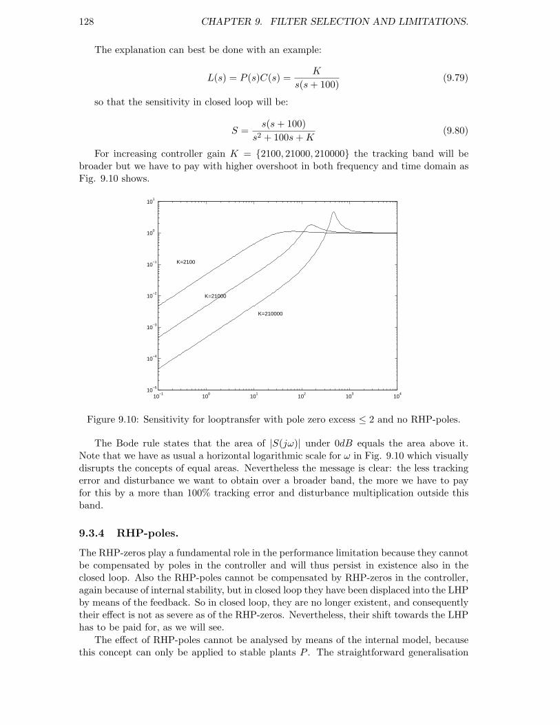
128 CHAPTER 9. FILTER SELECTION AND LIMITATIONS.
The explanation can best be done with an example:
L(s) = P (s)C(s) =K
s(s+ 100)(9.79)
so that the sensitivity in closed loop will be:
S =s(s+ 100)
s2 + 100s+K(9.80)
For increasing controller gain K = 2100, 21000, 210000 the tracking band will bebroader but we have to pay with higher overshoot in both frequency and time domain asFig. 9.10 shows.
10−1
100
101
102
103
104
10−5
10−4
10−3
10−2
10−1
100
101
K=2100
K=21000
K=210000
Figure 9.10: Sensitivity for looptransfer with pole zero excess ≤ 2 and no RHP-poles.
The Bode rule states that the area of |S(jω)| under 0dB equals the area above it.Note that we have as usual a horizontal logarithmic scale for ω in Fig. 9.10 which visuallydisrupts the concepts of equal areas. Nevertheless the message is clear: the less trackingerror and disturbance we want to obtain over a broader band, the more we have to payfor this by a more than 100% tracking error and disturbance multiplication outside thisband.
9.3.4 RHP-poles.
The RHP-zeros play a fundamental role in the performance limitation because they cannotbe compensated by poles in the controller and will thus persist in existence also in theclosed loop. Also the RHP-poles cannot be compensated by RHP-zeros in the controller,again because of internal stability, but in closed loop they have been displaced into the LHPby means of the feedback. So in closed loop, they are no longer existent, and consequentlytheir effect is not as severe as of the RHP-zeros. Nevertheless, their shift towards the LHPhas to be paid for, as we will see.
The effect of RHP-poles cannot be analysed by means of the internal model, becausethis concept can only be applied to stable plants P . The straightforward generalisation

9.3. LIMITATIONS DUE TO PLANT CHARACTERISTICS. 129
of the internal model for unstable plants has been explained in chapter 11. Essentially,the plant is first fed back for stabilisation and next an extra external loop with a stablecontroller Q is applied for optimisation. So the idea is first stabilisation and on top of thatoptimisation of the stable closed loop. It will be clear that the extra effort of stabilisationhas to be paid for. The currency is the use of the actuator range. Part of the actuator rangewill be occupied for the stabilisation task so that less is left for the optimisation comparedwith a stable plant, where we can use the whole range of the actuator for optimisation.This can be illustrated by a simple example represented in Fig. 9.11.
K1
s± a
r u+
−
Figure 9.11: Example for stabilisation effort.
The plant has either a pole in RHP at a > 0 or a pole in LHP at −a < 0. Theproportional controller K is bounded by the range of |u| < umax, while the closed loopshould be able to track a unit step. The control sensitivity is given by:
R =r
u=
K
1 + Ks±a
=K(s± a)s± a+K
(9.81)
For stability we certainly need K > a. The maximum |u| for a unit step occurs att = 0 so:
maxt
(u) = u(0) = lims→∞R(s) = K = umax (9.82)
So it is immediately clear that, limited by the actuator saturation, the pole in closedloop can maximally be shifted umax to the left. Consequently, for the unstable plant, apart a is used for stabilisation of the plant and only the remainder K − a can be used fora bandwidth K − a as illustrated in Fig. 9.12.
XXa−a
∗∗
K = umax
K = umax
<<−K − a −K + a
Figure 9.12: Rootloci for both plants 1/(s± a).
Note that the actuator range should be large enough, i.e. umax > a. Otherwisestabilisation is not possible. It defines a lower bound on K > a. With the same effortwe obtain a tracking band of K + a for the stable plant. Also the final error for the stepresponse is smaller:
e = Sr ⇒ e(∞) = lims→0
s± as± a+K
=±a
K ± a (9.83)
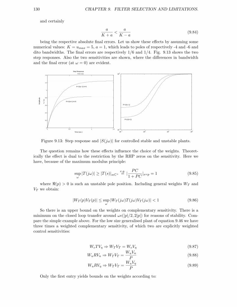
130 CHAPTER 9. FILTER SELECTION AND LIMITATIONS.
and certainly
a
K + a<
a
K − a (9.84)
being the respective absolute final errors. Let us show these effects by assuming somenumerical values: K = umax = 5, a = 1, which leads to poles of respectively -4 and -6 anddito bandwidths. The final errors are respectively 1/6 and 1/4. Fig. 9.13 shows the twostep responses. Also the two sensitivities are shown, where the differences in bandwidthand the final error (at ω = 0) are evident.
Time (sec.)
Am
plitu
de
Step Response
0 0.5 1 1.50
0.2
0.4
0.6
0.8
1
1.2
1.4From: U(1)
To:
Y(1
)
P=1/(s+1) K=5
P=1/(s−1) K=5
10−1
100
101
102
10−1
100
P=1/(s−1)
P=1/(s+1)
Figure 9.13: Step response and |S(jω)| for controlled stable and unstable plants.
The question remains how these effects influence the choice of the weights. Theoret-ically the effect is dual to the restriction by the RHP zeros on the sensitivity. Here wehave, because of the maximum modulus principle:
supω|T (jω)| ≥ |T (s)|sεC+
e.g.= | PC
1 + PC|s=p = 1 (9.85)
where (p) > 0 is such an unstable pole position. Including general weights WT andVT we obtain:
|WT (p)VT (p)| ≤ supω|WT (jω)T (jω)VT (jω)| < 1 (9.86)
So there is an upper bound on the weights on complementary sensitivity. There is aminimum on the closed loop transfer around ωε(|p|/2, 2|p|) for reasons of stability. Com-pare the simple example above. For the low size generalised plant of equation 9.46 we havethree times a weighted complementary sensitivity, of which two are explicitly weightedcontrol sensitivities:
WeTVη ⇒WTVT = WeVη (9.87)
WuRVn ⇒WTVT =WuVn
P(9.88)
WuRVη ⇒WTVT =WuVη
P(9.89)
Only the first entry yields bounds on the weights according to:
9.3. LIMITATIONS DUE TO PLANT CHARACTERISTICS. 131
|We(p)Vη((p)| < 1 (9.90)
because for the other two holds:
|Wu(p)Vn∪η(p)P (p)
| = 0 < 1 (9.91)
as |P (p)| =∞.The condition of inequality 9.90 is only a poor condition, because measurement noise
is usually very small. This is not the effect we are looking for, but alas I have not beenable to find it explicitly. You are invited to express the stabilisation effort explicitly in theweights.
In the Bode integral the effect of RHP-poles is evident, because if we have Np unstablepoles pi the Bode integral changes into:∫ ∞
0ln |S(jω)|dω = πΣNp
i=1(pi) (9.92)
which says that there is an extra positive area for ln |S| given by the sum of the realparts of the unstable poles multiplied by π. This is exactly the cost of the stabilisationand increases the further away the poles are from the imaginary axis. It implicitly statesthat we have to choose We such that there is left room for S in the nontracking band tobuild up this extra positive area where tracking and disturbance rejection are worse than100%.
Also in time domain we have a restriction on the step response, resembling the Bodeintegral in frequency domain (see Engell [16]). Let the open loop transfer have an unstablepole at p, so that we may write:
1 = T (p) =∫ ∞
0g(t)e−ptdt (9.93)
according to the Laplace transform of the closed loop impulse response g(t). Let thestep response be h(t) so that g(t) = dh(t)/dt. Then integration by parts yields:
1 =∫ ∞
0g(t)e−ptdt =
∫ ∞
0e−ptdh(t) = (9.94)
= h(t)e−pt|∞0 −∫ ∞
0h(t)de−pt = (9.95)
= p
∫ ∞
0h(t)e−ptdt (9.96)
where we used that h(0) = 0 when the closed loop system is strictly proper and thath(∞) is finite. Because it is straightforward that∫ ∞
0e−ptdt = −1
p
∫ ∞
0de−pt = −e
−pt
p|∞0 =
1p
(9.97)
the combination yields the restrictive time integral:∫ ∞
01− h(t)e−ptdt = 0 (9.98)
Equation 9.98 restricts the attainable step responses: the integral of the step responseerror, weighted by e−pt must vanish. As h(t) is below 1 for small values of t, this area must
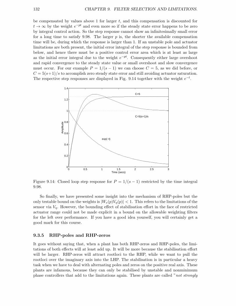
132 CHAPTER 9. FILTER SELECTION AND LIMITATIONS.
be compensated by values above 1 for larger t, and this compensation is discounted fort → ∞ by the weight e−pt and even more so if the steady state error happens to be zeroby integral control action. So the step response cannot show an infinitesimally small errorfor a long time to satisfy 9.98. The larger p is, the shorter the available compensationtime will be, during which the response is larger than 1. If an unstable pole and actuatorlimitations are both present, the initial error integral of the step response is bounded frombelow, and hence there must be a positive control error area which is at least as largeas the initial error integral due to the weight e−pt. Consequently either large overshootand rapid convergence to the steady state value or small overshoot and slow convergencemust occur. For our example P = 1/(s − 1) we can choose C = 5, as we did before, orC = 5(s+1)/s to accomplish zero steady state error and still avoiding actuator saturation.The respective step responses are displayed in Fig. 9.14 together with the weight e−t.
0 0.5 1 1.5 2 2.5 30
0.2
0.4
0.6
0.8
1
1.2
1.4
Time (secs)
Am
plitu
de
exp(−t)
C=5(s+1)/s
C=5
Figure 9.14: Closed loop step response for P = 1/(s − 1) restricted by the time integral9.98.
So finally, we have presented some insight into the mechanism of RHP-poles but theonly testable bound on the weights is |We(p)Vη(p)| < 1. This refers to the limitations of thesensor via Vη. However, the bounding effect of stabilisation effort in the face of restrictedactuator range could not be made explicit in a bound on the allowable weighting filtersfor the left over performance. If you have a good idea yourself, you will certainly get agood mark for this course.
9.3.5 RHP-poles and RHP-zeros
It goes without saying that, when a plant has both RHP-zeros and RHP-poles, the limi-tations of both effects will at least add up. It will be more because the stabilisation effortwill be larger. RHP-zeros will attract rootloci to the RHP, while we want to pull therootloci over the imaginary axis into the LHP. The stabilisation is in particular a heavytask when we have to deal with alternating poles and zeros on the positive real axis. Theseplants are infamous, because they can only be stabilised by unstable and nonminimumphase controllers that add to the limitations again. These plants are called ”not strongly

9.3. LIMITATIONS DUE TO PLANT CHARACTERISTICS. 133
stabilisable”. Take for instance a plant with a zero z > 0, p > 0 and an integrator pole at0. If z < p we have alternatingly poles and zeros at 0, z, p and ∞. Depending on the signof the controller gain K, and no poles or zeros of the controller on the positive real axis,the rootloci will always remain in the RHP as displayed in Fig. 9.15.
X XO ><><K > 0 K < 0 K > 0 K < 0
z p0
Figure 9.15: Rootloci for a plant, which is not strongly stabilisable.
Only if we add RHP-zeros and RHP-poles in the controller such that we alternatinglyhave pairs of zeros and poles on the real positive axis we can accomplish that the rootlocileave the real positive axis and can be drawn to the LHP as illustrated in Fig. 9.16.
X XO ><><K > 0 K < 0 K < 0 K < 0
z p0O X
K > 0K > 0
Figure 9.16: Rootloci for a plant, which is not strongly stabilisable, with an unstablenonminimum phase controller.
It will be clear that this stabilisation effort is considerable and the more if the RHP-poles and RHP-zeros are close to each other so that without precautions the open ends ofthe rootloci leaving and approaching the real positive axis in Fig. 9.16 will close withoutpassing through the LHP first. In Skogestadt & Postlethwaite [15] this is formalised inthe following bounding theorem:
Theorem: Combined RHP-poles and RHP-zeros. Suppose that P (s) has Nz
RHP-zeros zj and has Np RHP-poles pi. Then for closed-loop stability the weighted sensi-tivity function must satisfy for each RHP-zero zj:
‖WSSVS ‖∞≥ c1j |WS(zj)VS(zj)|, c1j = ΠNp
i=1|zj + pi||zj − pi| ≥ 1 (9.99)
and the weighted complementary sensitivity function must satisfy for each RHP-polepi:
‖WTTVT ‖∞≥ c2j |WT (pi)VT (pi)|, c2j = ΠNzj=1|zj + pi||zj − pi| ≥ 1 (9.100)

134 CHAPTER 9. FILTER SELECTION AND LIMITATIONS.
where WS and VS are sensitivity weighting filters like the pair We, Vn. Similarly,WT and VT are complementary sensitivity weighting filters like the pair We, Vη. If wewant the infinity norms to be less than γ ≈ 1, above inequalities put upper bounds on theweight filters. On the other hand if we apply the theorem without weights we get:
‖ S ‖∞≥ maxjc1j ‖ T ‖∞≥ max
ic2i (9.101)
This shows that large peaks for S and T are unavoidable if we have a RHP-pole andRHP-zero located close to each other.
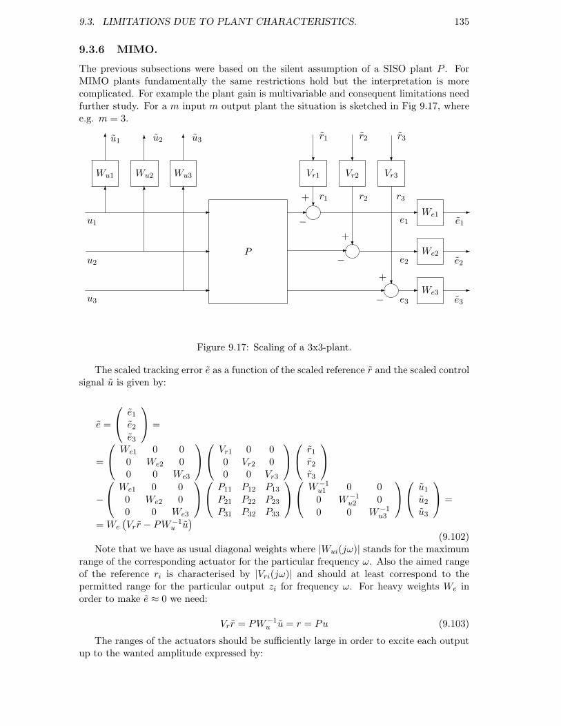
9.3. LIMITATIONS DUE TO PLANT CHARACTERISTICS. 135
9.3.6 MIMO.
The previous subsections were based on the silent assumption of a SISO plant P . ForMIMO plants fundamentally the same restrictions hold but the interpretation is morecomplicated. For example the plant gain is multivariable and consequent limitations needfurther study. For a m input m output plant the situation is sketched in Fig 9.17, wheree.g. m = 3.
We3
We2
We1
Vr3Vr2Vr1
P
Wu3Wu2Wu1
u1 u2 u3
u1
u2
u3
r1 r2 r3
e1
e2
e3
e1
e2
e3
r1 r2 r3+
+
+
−
−
−
Figure 9.17: Scaling of a 3x3-plant.
The scaled tracking error e as a function of the scaled reference r and the scaled controlsignal u is given by:
e =
e1e2e3
=
=
We1 0 00 We2 00 0 We3
Vr1 0 00 Vr2 00 0 Vr3
r1r2r3
− We1 0 0
0 We2 00 0 We3
P11 P12 P13P21 P22 P23P31 P32 P33
W−1u1 0 00 W−1
u2 00 0 W−1
u3
u1u2u3
=
= We
(Vrr − PW−1
u u)
(9.102)Note that we have as usual diagonal weights where |Wui(jω)| stands for the maximum
range of the corresponding actuator for the particular frequency ω. Also the aimed rangeof the reference ri is characterised by |Vri(jω)| and should at least correspond to thepermitted range for the particular output zi for frequency ω. For heavy weights We inorder to make e ≈ 0 we need:
Vrr = PW−1u u = r = Pu (9.103)
The ranges of the actuators should be sufficiently large in order to excite each outputup to the wanted amplitude expressed by:
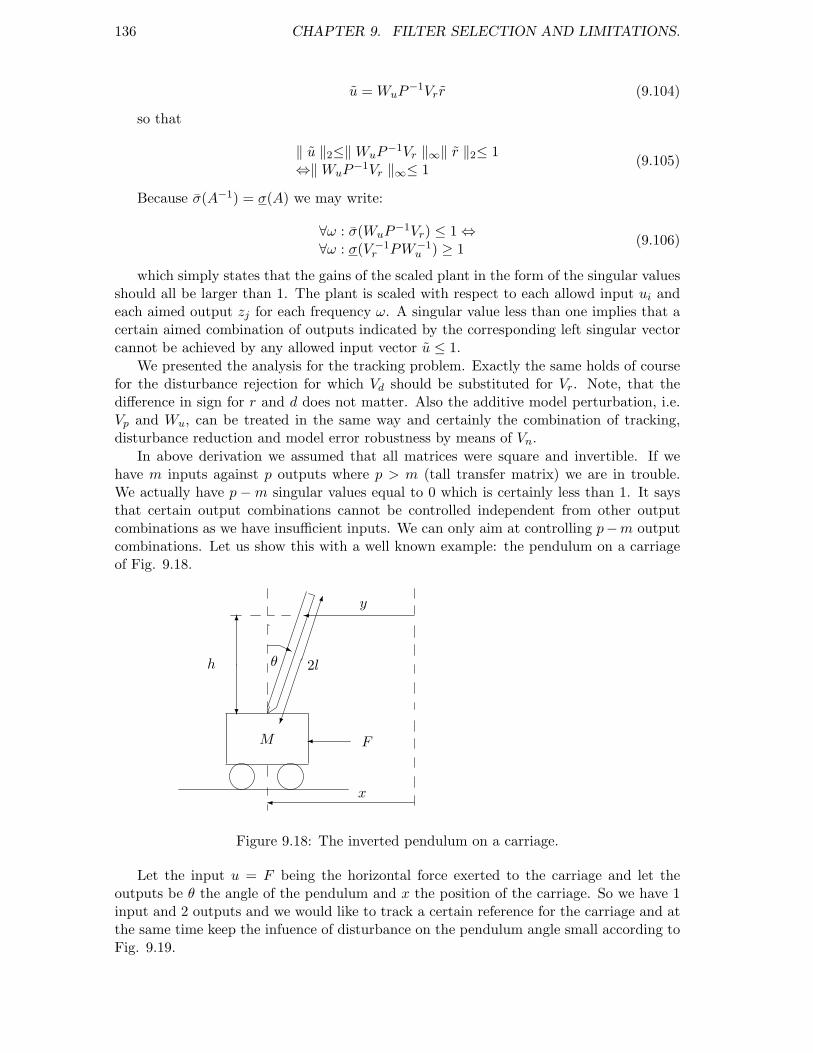
136 CHAPTER 9. FILTER SELECTION AND LIMITATIONS.
u = WuP−1Vrr (9.104)
so that
‖ u ‖2≤‖WuP−1Vr ‖∞‖ r ‖2≤ 1
⇔‖WuP−1Vr ‖∞≤ 1
(9.105)
Because σ(A−1) = σ(A) we may write:
∀ω : σ(WuP−1Vr) ≤ 1⇔
∀ω : σ(V −1r PW−1
u ) ≥ 1(9.106)
which simply states that the gains of the scaled plant in the form of the singular valuesshould all be larger than 1. The plant is scaled with respect to each allowd input ui andeach aimed output zj for each frequency ω. A singular value less than one implies that acertain aimed combination of outputs indicated by the corresponding left singular vectorcannot be achieved by any allowed input vector u ≤ 1.
We presented the analysis for the tracking problem. Exactly the same holds of coursefor the disturbance rejection for which Vd should be substituted for Vr. Note, that thedifference in sign for r and d does not matter. Also the additive model perturbation, i.e.Vp and Wu, can be treated in the same way and certainly the combination of tracking,disturbance reduction and model error robustness by means of Vn.
In above derivation we assumed that all matrices were square and invertible. If wehave m inputs against p outputs where p > m (tall transfer matrix) we are in trouble.We actually have p −m singular values equal to 0 which is certainly less than 1. It saysthat certain output combinations cannot be controlled independent from other outputcombinations as we have insufficient inputs. We can only aim at controlling p−m outputcombinations. Let us show this with a well known example: the pendulum on a carriageof Fig. 9.18.
M
θh
y
F
x
2l
Figure 9.18: The inverted pendulum on a carriage.
Let the input u = F being the horizontal force exerted to the carriage and let theoutputs be θ the angle of the pendulum and x the position of the carriage. So we have 1input and 2 outputs and we would like to track a certain reference for the carriage and atthe same time keep the infuence of disturbance on the pendulum angle small according toFig. 9.19.
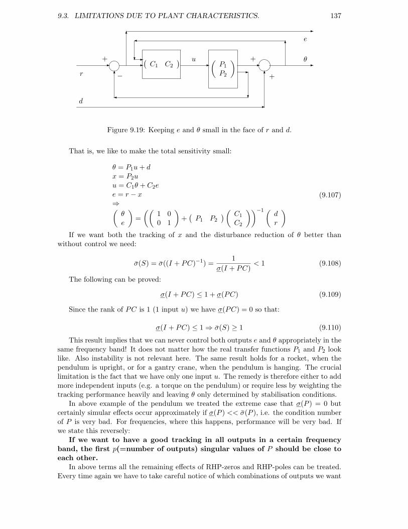
9.3. LIMITATIONS DUE TO PLANT CHARACTERISTICS. 137
(P1P2
)(C1 C2
)
r
d
+
−
u +
+
θ
e
Figure 9.19: Keeping e and θ small in the face of r and d.
That is, we like to make the total sensitivity small:
θ = P1u+ dx = P2uu = C1θ + C2ee = r − x⇒(θe
)=((
1 00 1
)+(P1 P2
)( C1C2
))−1(dr
) (9.107)
If we want both the tracking of x and the disturbance reduction of θ better thanwithout control we need:
σ(S) = σ((I + PC)−1) =1
σ(I + PC)< 1 (9.108)
The following can be proved:
σ(I + PC) ≤ 1 + σ(PC) (9.109)
Since the rank of PC is 1 (1 input u) we have σ(PC) = 0 so that:
σ(I + PC) ≤ 1⇒ σ(S) ≥ 1 (9.110)
This result implies that we can never control both outputs e and θ appropriately in thesame frequency band! It does not matter how the real transfer functions P1 and P2 looklike. Also instability is not relevant here. The same result holds for a rocket, when thependulum is upright, or for a gantry crane, when the pendulum is hanging. The cruciallimitation is the fact that we have only one input u. The remedy is therefore either to addmore independent inputs (e.g. a torque on the pendulum) or require less by weighting thetracking performance heavily and leaving θ only determined by stabilisation conditions.
In above example of the pendulum we treated the extreme case that σ(P ) = 0 butcertainly simular effects occur approximately if σ(P ) << σ(P ), i.e. the condition numberof P is very bad. For frequencies, where this happens, performance will be very bad. Ifwe state this reversely:
If we want to have a good tracking in all outputs in a certain frequencyband, the first p(=number of outputs) singular values of P should be close toeach other.
In above terms all the remaining effects of RHP-zeros and RHP-poles can be treated.Every time again we have to take careful notice of which combinations of outputs we want

138 CHAPTER 9. FILTER SELECTION AND LIMITATIONS.
to control and what combinations of inputs we can use therefore. These combinationsfind their representation in characteristic vectors like singular vectors and eigenvectors.Sometimes this relieves the control task as certain ”difficult” vectors are irrelevant for thecontrol job, sometimes it is just the opposite as a ”difficult” vector appears to be crucialfor the control task. This makes the complete analysis a rather extensive task, too big forthe limited course we are involved in. Therefore we refer to e.g. Skogestadt [15] for moredetails.
9.4 Summary
Before passing on to an example where we apply above rules together with the program-ming instructions, it seems worthwhile to summarise the features here.
A procedure for the set up can be described as:
1. Define the proposed control structure. Try to combine as many inputs as possiblein an augmented plant.
2. Analyse the exogenous signals such that the characterising filters V∗ can be givennumerical values.
3. Analyse the actuator bounds for each frequency, yielding the Wu.
4. Analyse the model perturbations and try to ”catch” them with input filters V∗ andWu. If not possible, enlarge some weights or add others e.g. Wz for multiplicativeerrors.
5. Propose a filter We for performance.
6. Test whether S + T = I is not violated by the set of weights and adapt We ifnecessary.
7. Program the problem and try to find ‖M ‖∞< γ ≈ 1.
At this stage one often meets difficulties as the programs cannot even find any gammaat all, as their are problems before. The following anomalies are often encountered, oncethe augmented plant (see chapter 13) has been obtained:
x = Ax+B1w +B2u
z = C1x+D11w +D12u
y = C2x+D21w +D22u
(9.111)
1. (A,B2) is not stabilisable. Unstable modes cannot be controlled. Usually not welldefined plant. Be sure that all your weights are stable and minimum phase.
2. (A,C2) is not detectable. Unstable modes cannot be observed. Usually not welldefined plant. Again, all your weights should be stable and minimum phase.
3. D12 does not have full rank equal to the number of inputs ui. This means that notall inputs ui are penalised in the outputs z by means of the weights Wui. Theyshould be penalised for all frequencies so that biproper weights Wui are required. Ifnot all ui are weighted for all frequencies, the effect is the same as when we have inLQG-control a weight matrix R which is singular and needs to be inverted in thesolution algorithm. In chapter 13 we saw that for the LQG-problem D12 = R
12 .
9.4. SUMMARY 139
4. D21 does not have full rank equal to the number of measured outputs yj . This is dualto the previous item. It means that not all measurements are polluted by ”noise”,i.e. the exogenous inputs w. Noise-free measurements cannot exist as they wouldbe infinitely reliable. So, for each frequency there should be some disturbance, i.e.direct feedthrough from w. Usually the problem is solved by making all exogenousinput filters V∗ biproper. Next, one should investigate whether the problem definitionis realistic and some measurement noise should be added. If one does not want toincrease the number of inputs wi, one can search for a proper entry in D21 and giveit a very small value, thereby fooling the algorithm without influencing the resultseriously. The lack of full rank is comparable again with LQG-control, when thecovariance matrix of the measurement noise is singular. In chapter 13 we saw that
for the LQG-problem D21 = R12w.
5. Numerical problems occur, the accuracy appears to be insufficient. Quite often thisis due to too broad a frequency band where all dynamics should be considered. Besure that all poles and zeros in absolute value do not cover more than 5 decades.In particular the biproperness requirement induced by the two previous items mayhave set you to trespass the 5 decades or the integration pole, which you have wiselyshifted somewhat in the LHP is still too small compared to the largest pole or zero.
Supposing, that, based on above hints, you have indeed obtained a γ which is farexceeding one, however, the following tests in the proposed order can be done for findingthe underlying reason:
1. Test for the fundamental equality S + T = I again, whether the respective weightsintersect below 0dB.
2. Test for sufficient plant gain(s) by ∀ω : σ(V −1∗ PW−1u ) ≥ 1 with V∗ = Vr or Vd or Vn.
3. In case of RHP-zeros z test |We(z)V∗(z)| < 1 withV∗ = Vr or Vd or Vn.
4. In case of RHP-poles p test |We(p)Vη(p)| < 1
5. Test whether sufficient room is left for the sensitivity by its weights to satisfy thebode integral, in particular in case of RHP-poles pj :∫ ∞
0ln |S(jω)|dω = πΣNp
i=1(pi) (9.112)
6. In case of both RHP-poles and RHP-zeros test on basis of theorem equations 9.99and 9.100.
Still no solution? Find an expert.

140 CHAPTER 9. FILTER SELECTION AND LIMITATIONS.
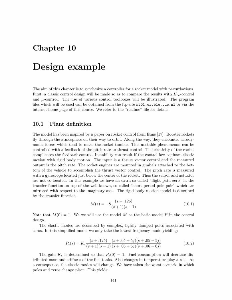
Chapter 10
Design example
The aim of this chapter is to synthesize a controller for a rocket model with perturbations.First, a classic control design will be made so as to compare the results with H∞-controland µ-control. The use of various control toolboxes will be illustrated. The programfiles which will be used can be obtained from the ftp-site nt01.er.ele.tue.nl or via theinternet home page of this course. We refer to the “readme” file for details.
10.1 Plant definition
The model has been inspired by a paper on rocket control from Enns [17]. Booster rocketsfly through the atmosphere on their way to orbit. Along the way, they encounter aerody-namic forces which tend to make the rocket tumble. This unstable phenomenon can becontrolled with a feedback of the pitch rate to thrust control. The elasticity of the rocketcomplicates the feedback control. Instability can result if the control law confuses elasticmotion with rigid body motion. The input is a thrust vector control and the measuredoutput is the pitch rate. The rocket engines are mounted in gimbals attached to the bot-tom of the vehicle to accomplish the thrust vector control. The pitch rate is measuredwith a gyroscope located just below the center of the rocket. Thus the sensor and actuatorare not co-located. In this example we have an extra so called “flight path zero” in thetransfer function on top of the well known, so called “short period pole pair” which aremirrored with respect to the imaginary axis. The rigid body motion model is describedby the transfer function
M(s) = −8(s+ .125)
(s+ 1)(s− 1)(10.1)
Note that M(0) = 1. We we will use the model M as the basic model P in the controldesign.
The elastic modes are described by complex, lightly damped poles associated withzeros. In this simplified model we only take the lowest frequency mode yielding:
Ps(s) = Ks(s+ .125)
(s+ 1)(s− 1)(s+ .05 + 5j)(s+ .05− 5j)(s+ .06 + 6j)(s+ .06− 6j)
(10.2)
The gain Ks is determined so that Ps(0) = 1. Fuel consumption will decrease dis-tributed mass and stiffness of the fuel tanks. Also changes in temperature play a role. Asa consequence, the elastic modes will change. We have taken the worst scenario in whichpoles and zeros change place. This yields:
141
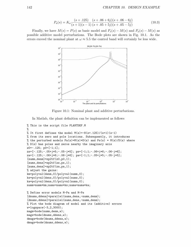
142 CHAPTER 10. DESIGN EXAMPLE
Pa(s) = Ka(s+ .125)
(s+ 1)(s− 1)(s+ .06 + 6j)(s+ .06− 6j)(s+ .05 + 5j)(s+ .05− 5j)
(10.3)
Finally, we have M(s) = P (s) as basic model and Ps(s)−M(s) and Pa(s)−M(s) aspossible additive model perturbations. The Bode plots are shown in Fig. 10.1. As theerrors exceed the nominal plant at ω ≈ 5.5 the control band will certainly be less wide.
10−3
10−2
10−1
100
101
102
10−7
10−6
10−5
10−4
10−3
10−2
10−1
100
101
102
|M|,|M−Ps|,|M−Pa|
The plant and its perturbations
Figure 10.1: Nominal plant and additive perturbations.
In Matlab, the plant definition can be implemented as follows
% This is the script file PLANTDEF.M%% It first defines the model M(s)=-8(s+.125)/(s+1)(s-1)% from its zero and pole locations. Subsequently, it introduces% the perturbed models Pa(s)=M(s)*D(s) and Ps(s) = M(s)/D(s) where% D(s) has poles and zeros nearby the imaginary axisz0=-.125; p0=[-1;1];zs=[-.125;-.05+j*5;-.05-j*5]; ps=[-1;1;-.06+j*6;-.06-j*6];za=[-.125;-.06+j*6;-.06-j*6]; pa=[-1;1;-.05+j*5;-.05-j*5];[numm,denm]=zp2tf(z0,p0,1);[nums,dens]=zp2tf(zs,ps,1);[numa,dena]=zp2tf(za,pa,1);% adjust the gains:km=polyval(denm,0)/polyval(numm,0);ks=polyval(dens,0)/polyval(nums,0);ka=polyval(dena,0)/polyval(numa,0);numm=numm*km;nums=nums*ks;numa=numa*ka;
% Define error models M-Pa and M-Ps[dnuma,ddena]=parallel(numa,dena,-numm,denm);[dnums,ddens]=parallel(nums,dens,-numm,denm);% Plot the bode diagram of model and its (additive) errorsw=logspace(-3,2,3000);magm=bode(numm,denm,w);mags=bode(dnums,ddens,w);dmaga=bode(dnuma,ddena,w);dmags=bode(dnums,ddens,w);
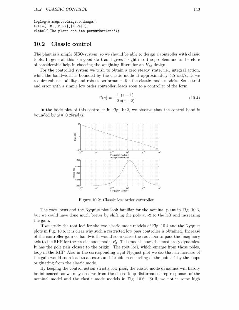
10.2. CLASSIC CONTROL 143
loglog(w,magm,w,dmags,w,dmaga);title(’|M|,|M-Ps|,|M-Pa|’);xlabel(’The plant and its perturbations’);
10.2 Classic control
The plant is a simple SISO-system, so we should be able to design a controller with classictools. In general, this is a good start as it gives insight into the problem and is thereforeof considerable help in choosing the weighting filters for an H∞-design.
For the controlled system we wish to obtain a zero steady state, i.e., integral action,while the bandwidth is bounded by the elastic mode at approximately 5.5 rad/s, as werequire robust stability and robust performance for the elastic mode models. Some trialand error with a simple low order controller, leads soon to a controller of the form
C(s) = −12
(s+ 1)s(s+ 2)
(10.4)
In the bode plot of this controller in Fig. 10.2, we observe that the control band isbounded by ω ≈ 0.25rad/s.
10−3
10−2
10−1
100
101
102
−50
0
50
Frequency (rad/sec)
Gai
n dB
10−3
10−2
10−1
100
101
102
−270
−265
−260
−255
−250
Frequency (rad/sec)
Pha
se d
eg
bodeplots controller
Figure 10.2: Classic low order controller.
The root locus and the Nyquist plot look familiar for the nominal plant in Fig. 10.3,but we could have done much better by shifting the pole at -2 to the left and increasingthe gain.
If we study the root loci for the two elastic mode models of Fig. 10.4 and the Nyquistplots in Fig. 10.5, it is clear why such a restricted low pass controller is obtained. Increaseof the controller gain or bandwidth would soon cause the root loci to pass the imaginaryaxis to the RHP for the elastic mode model Pa. This model shows the most nasty dynamics.It has the pole pair closest to the origin. The root loci, which emerge from those poles,loop in the RHP. Also in the corresponding right Nyquist plot we see that an increase ofthe gain would soon lead to an extra and forbidden encircling of the point -1 by the loopsoriginating from the elastic mode.
By keeping the control action strictly low pass, the elastic mode dynamics will hardlybe influenced, as we may observe from the closed loop disturbance step responses of thenominal model and the elastic mode models in Fig. 10.6. Still, we notice some high
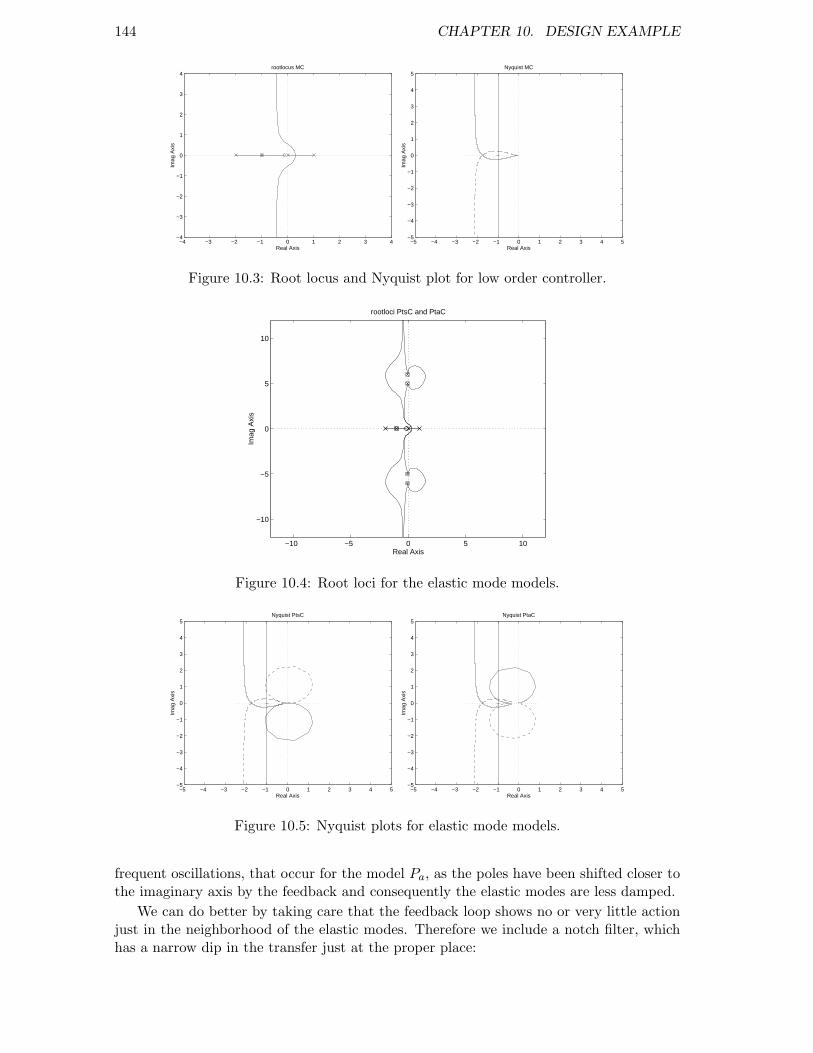
144 CHAPTER 10. DESIGN EXAMPLE
−4 −3 −2 −1 0 1 2 3 4−4
−3
−2
−1
0
1
2
3
4
Real Axis
Imag
Axi
s
rootlocus MC
−5 −4 −3 −2 −1 0 1 2 3 4 5−5
−4
−3
−2
−1
0
1
2
3
4
5
Real Axis
Imag
Axi
s
Nyquist MC
Figure 10.3: Root locus and Nyquist plot for low order controller.
−10 −5 0 5 10
−10
−5
0
5
10
Real Axis
Imag
Axi
s
rootloci PtsC and PtaC
Figure 10.4: Root loci for the elastic mode models.
−5 −4 −3 −2 −1 0 1 2 3 4 5−5
−4
−3
−2
−1
0
1
2
3
4
5
Real Axis
Imag
Axi
s
Nyquist PtsC
−5 −4 −3 −2 −1 0 1 2 3 4 5−5
−4
−3
−2
−1
0
1
2
3
4
5
Real Axis
Imag
Axi
s
Nyquist PtaC
Figure 10.5: Nyquist plots for elastic mode models.
frequent oscillations, that occur for the model Pa, as the poles have been shifted closer tothe imaginary axis by the feedback and consequently the elastic modes are less damped.
We can do better by taking care that the feedback loop shows no or very little actionjust in the neighborhood of the elastic modes. Therefore we include a notch filter, whichhas a narrow dip in the transfer just at the proper place:
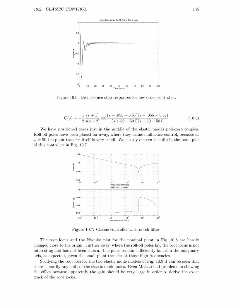
10.2. CLASSIC CONTROL 145
0 10 20 30 40 50 60 70 80 90 100−2
−1.5
−1
−0.5
0
0.5
1
Time (secs)
Am
plitu
de
step disturbance for M, Pts or Pta in loop
Figure 10.6: Disturbance step responses for low order controller.
C(s) = −12
(s+ 1)s(s+ 2)
150(s+ .055 + 5.5j)(s+ .055− 5.5j)
(s+ 50 + 50j)(s+ 50− 50j)(10.5)
We have positioned zeros just in the middle of the elastic modes pole-zero couples.Roll off poles have been placed far away, where they cannot influence control, because atω = 50 the plant transfer itself is very small. We clearly discern this dip in the bode plotof this controller in Fig. 10.7.
10−3
10−2
10−1
100
101
102
−100
−50
0
50
Frequency (rad/sec)
Gai
n dB
10−3
10−2
10−1
100
101
102
−90
−180
−270
0
Frequency (rad/sec)
Pha
se d
eg
bodeplots controller
Figure 10.7: Classic controller with notch filter.
The root locus and the Nyquist plot for the nominal plant in Fig. 10.8 are hardlychanged close to the origin. Further away, where the roll-off poles lay, the root locus is notinteresting and has not been shown. The poles remain sufficiently far from the imaginaryaxis, as expected, given the small plant transfer at those high frequencies.
Studying the root loci for the two elastic mode models of Fig. 10.9 it can be seen thatthere is hardly any shift of the elastic mode poles. Even Matlab had problems in showingthe effect because apparently the gain should be very large in order to derive the exacttrack of the root locus.
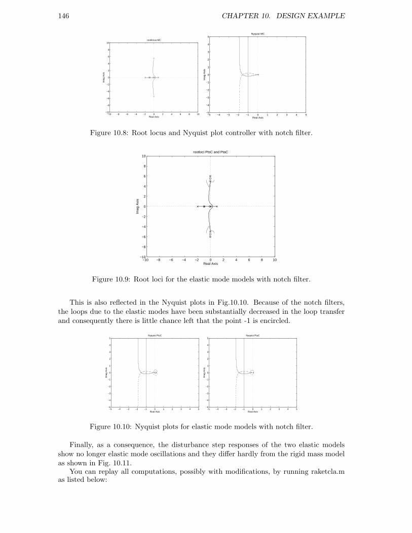
146 CHAPTER 10. DESIGN EXAMPLE
−10 −8 −6 −4 −2 0 2 4 6 8 10−10
−8
−6
−4
−2
0
2
4
6
8
10
Real Axis
Imag
Axi
s
rootlocus MC
−5 −4 −3 −2 −1 0 1 2 3 4 5−5
−4
−3
−2
−1
0
1
2
3
4
5
Real Axis
Imag
Axi
s
Nyquist MC
Figure 10.8: Root locus and Nyquist plot controller with notch filter.
−10 −8 −6 −4 −2 0 2 4 6 8 10−10
−8
−6
−4
−2
0
2
4
6
8
10
Real Axis
Imag
Axi
s
rootloci PtsC and PtaC
Figure 10.9: Root loci for the elastic mode models with notch filter.
This is also reflected in the Nyquist plots in Fig.10.10. Because of the notch filters,the loops due to the elastic modes have been substantially decreased in the loop transferand consequently there is little chance left that the point -1 is encircled.
−5 −4 −3 −2 −1 0 1 2 3 4 5−5
−4
−3
−2
−1
0
1
2
3
4
5
Real Axis
Imag
Axi
s
Nyquist PtsC
−5 −4 −3 −2 −1 0 1 2 3 4 5−5
−4
−3
−2
−1
0
1
2
3
4
5
Real Axis
Imag
Axi
s
Nyquist PtaC
Figure 10.10: Nyquist plots for elastic mode models with notch filter.
Finally, as a consequence, the disturbance step responses of the two elastic modelsshow no longer elastic mode oscillations and they differ hardly from the rigid mass modelas shown in Fig. 10.11.
You can replay all computations, possibly with modifications, by running raketcla.mas listed below:
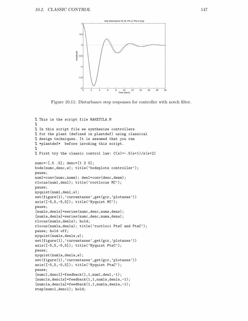
10.2. CLASSIC CONTROL 147
0 2 4 6 8 10 12 14 16 18 20−2
−1.5
−1
−0.5
0
0.5
1
Time (secs)
Am
plitu
de
step disturbance for M, Pts or Pta in loop
Figure 10.11: Disturbance step responses for controller with notch filter.
% This is the script file RAKETCLA.M%% In this script file we synthesize controllers% for the plant (defined in plantdef) using classical% design techniques. It is assumed that you ran% *plantdef* before invoking this script.%% First try the classic control law: C(s)=-.5(s+1)/s(s+2)
numc=-[.5 .5]; denc=[1 2 0];bode(numc,denc,w); title(’bodeplots controller’);pause;numl=conv(numc,numm); denl=conv(denc,denm);rlocus(numl,denl); title(’rootlocus MC’);pause;nyquist(numl,denl,w);set(figure(1),’currentaxes’,get(gcr,’plotaxes’))axis([-5,5,-5,5]); title(’Nyquist MC’);pause;[numls,denls]=series(numc,denc,nums,dens);[numla,denla]=series(numc,denc,numa,dena);rlocus(numls,denls); hold;rlocus(numla,denla); title(’rootloci PtsC and PtaC’);pause; hold off;nyquist(numls,denls,w);set(figure(1),’currentaxes’,get(gcr,’plotaxes’))axis([-5,5,-5,5]); title(’Nyquist PtsC’);pause;nyquist(numla,denla,w);set(figure(1),’currentaxes’,get(gcr,’plotaxes’))axis([-5,5,-5,5]); title(’Nyquist PtaC’);pause;[numcl,dencl]=feedback(1,1,numl,denl,-1);[numcls,dencls]=feedback(1,1,numls,denls,-1);[numcla,dencla]=feedback(1,1,numla,denla,-1);step(numcl,dencl); hold;

148 CHAPTER 10. DESIGN EXAMPLE
step(numcls,dencls); step(numcla,dencla);title(’step disturbance for M, Pts or Pta in loop’);pause; hold off;
% Improved classic controller C(s)=[.5(s+1)/s(s+2)]*% 150(s+.055+j*5.5)(s+.055-j*5.5)/(s+50-j*50)(s+50-j*50)
numc=conv(-[.5 .5],[1 .1 30.2525]*150);denc=conv([1 2 0],[1 100 5000]);bode(numc,denc,w); title(’bodeplots controller’);pause;numl=conv(numc,numm); denl=conv(denc,denm);rlocus(numl,denl);axis([-10,10,-10,10]); title(’rootlocus MC’);pause;nyquist(numl,denl,w);set(figure(1),’currentaxes’,get(gcr,’plotaxes’))axis([-5,5,-5,5]); title(’Nyquist MC’);pause;[numls,denls]=series(numc,denc,nums,dens);[numla,denla]=series(numc,denc,numa,dena);rlocus(numls,denls); hold; rlocus(numla,denla);axis([-10,10,-10,10]); title(’rootloci PtsC and PtaC’);pause; hold off;nyquist(numls,denls,w);set(figure(1),’currentaxes’,get(gcr,’plotaxes’))axis([-5,5,-5,5]); title(’Nyquist PtsC’);pause;nyquist(numla,denla,w);set(figure(1),’currentaxes’,get(gcr,’plotaxes’))axis([-5,5,-5,5]); title(’Nyquist PtaC’);pause;[numcl,dencl]=feedback(1,1,numl,denl,-1);[numcls,dencls]=feedback(1,1,numls,denls,-1);[numcla,dencla]=feedback(1,1,numla,denla,-1);step(numcl,dencl);hold;step(numcls,dencls);step(numcla,dencla);title(’step disturbance for M, Pts or Pta in loop’);pause; hold off;
10.3 Augmented plant and weight filter selection
Being an example we want to keep the control design simple so that we propose a simplemixed sensitivity set-up as depicted in Fig. 10.12.
The exogenous input w = d stands in principle for the aerodynamic forces acting onthe rocket in flight for a nominal speed. It will also represent the model perturbationstogether with the weight on the actuator input u = u. The disturbed output of the rocket,the pitch rate, should be kept to zero as close as possible. Because we can see it as anerror, we incorporate it, in a weighted form e, as a component of the output z = (u, e)T .At the same time, the error e is used as the measurement y = e for the controller. Notethat we did not pay attention to measurement errors. The mixed sensitivity is thus definedby:
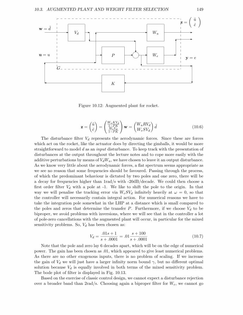
10.3. AUGMENTED PLANT AND WEIGHT FILTER SELECTION 149
K
P We
WuVd
G
w = d
u = u
z =(ue
)
y = e
Figure 10.12: Augmented plant for rocket.
z =(ue
)=
(WuKVd1−PKWeVd1−PK
)w =
(WuRVd
WeSVd
)d (10.6)
The disturbance filter Vd represents the aerodynamic forces. Since these are forceswhich act on the rocket, like the actuator does by directing the gimballs, it would be morestraightforward to model d as an input disturbance. To keep track with the presentation ofdisturbances at the output throughout the lecture notes and to cope more easily with theadditive perturbations by means of VdWu, we have chosen to leave it an output disturbance.As we know very little about the aerodynamic forces, a flat spectrum seems appropriate aswe see no reason that some frequencies should be favoured. Passing through the process,of which the predominant behaviour is dictated by two poles and one zero, there will bea decay for frequencies higher than 1rad/s with -20dB/decade. We could then choose afirst order filter Vd with a pole at -1. We like to shift the pole to the origin. In thatway we will penalise the tracking error via WeSVd infinitely heavily at ω = 0, so thatthe controller will necessarily contain integral action. For numerical reasons we have totake the integration pole somewhat in the LHP at a distance which is small compared tothe poles and zeros that determine the transfer P . Furthermore, if we choose Vd to bebiproper, we avoid problems with inversions, where we will see that in the controller a lotof pole-zero cancellations with the augmented plant will occur, in particular for the mixedsensitivity problems. So, Vd has been chosen as:
Vd =.01s+ 1s+ .0001
= .01s+ 100s+ .0001
(10.7)
Note that the pole and zero lay 6 decades apart, which will be on the edge of numericalpower. The gain has been chosen as .01, which appeared to give least numerical problems.As there are no other exogenous inputs, there is no problem of scaling. If we increasethe gain of Vd we will just have a larger infinity norm bound γ, but no different optimalsolution because Vd is equally involved in both terms of the mixed sensitivity problem.The bode plot of filter is displayed in Fig. 10.13.
Based on the exercise of classic control design, we cannot expect a disturbance rejectionover a broader band than 2rad/s. Choosing again a biproper filter for We, we cannot go
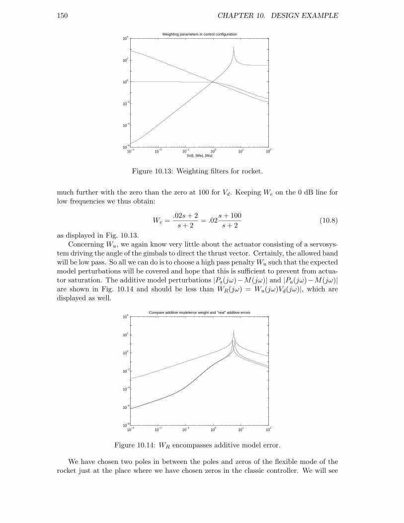
150 CHAPTER 10. DESIGN EXAMPLE
10−3
10−2
10−1
100
101
102
10−6
10−4
10−2
100
102
104
|Vd|, |We|, |Wu|
Weighting parameters in control configuration
Figure 10.13: Weighting filters for rocket.
much further with the zero than the zero at 100 for Vd. Keeping We on the 0 dB line forlow frequencies we thus obtain:
We =.02s+ 2s+ 2
= .02s+ 100s+ 2
(10.8)
as displayed in Fig. 10.13.Concerning Wu, we again know very little about the actuator consisting of a servosys-
tem driving the angle of the gimbals to direct the thrust vector. Certainly, the allowed bandwill be low pass. So all we can do is to choose a high pass penaltyWu such that the expectedmodel perturbations will be covered and hope that this is sufficient to prevent from actua-tor saturation. The additive model perturbations |Ps(jω)−M(jω)| and |Pa(jω)−M(jω)|are shown in Fig. 10.14 and should be less than WR(jω) = Wu(jω)Vd(jω)|, which aredisplayed as well.
10−3
10−2
10−1
100
101
102
10−8
10−6
10−4
10−2
100
102
104
Compare additive modelerror weight and "real" additive errors
Figure 10.14: WR encompasses additive model error.
We have chosen two poles in between the poles and zeros of the flexible mode of therocket just at the place where we have chosen zeros in the classic controller. We will see
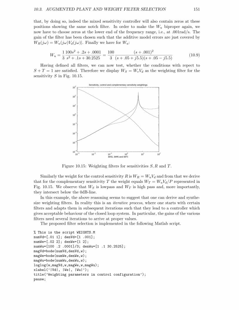
10.3. AUGMENTED PLANT AND WEIGHT FILTER SELECTION 151
that, by doing so, indeed the mixed sensitivity controller will also contain zeros at thesepositions showing the same notch filter. In order to make the Wu biproper again, wenow have to choose zeros at the lower end of the frequency range, i.e., at .001rad/s. Thegain of the filter has been chosen such that the additive model errors are just covered byWR(jω) = Wu(jω)Vd(jω)|. Finally we have for Wu:
Wu =13
100s2 + .2s+ .0001s2 + .1s+ 30.2525
=1003
(s+ .001)2
(s+ .05 + j5.5)(s+ .05− j5.5)(10.9)
Having defined all filters, we can now test, whether the conditions with repect toS + T = 1 are satisfied. Therefore we display WS = WeVd as the weighting filter for thesensitivity S in Fig. 10.15.
10−3
10−2
10−1
100
101
102
10−4
10−3
10−2
10−1
100
101
102
103
|WS|, |WR| and |WT|
Sensitivity, control and complementary sensitivity weightings
Figure 10.15: Weighting filters for sensitivities S,R and T .
Similarly the weight for the control sensitivityR isWR = WuVd and from that we derivethat for the complementary sensitivity T the weight equals WT = WuVd/P represented inFig. 10.15. We observe that WS is lowpass and WT is high pass and, more importantly,they intersect below the 0dB-line.
In this example, the above reasoning seems to suggest that one can derive and synthe-size weighting filters. In reality this is an iterative process, where one starts with certainfilters and adapts them in subsequent iterations such that they lead to a controller whichgives acceptable behaviour of the closed loop system. In particular, the gains of the variousfilters need several iterations to arrive at proper values.
The proposed filter selection is implemented in the following Matlab script.
% This is the script WEIGHTS.MnumVd=[.01 1]; denVd=[1 .001];numWe=[.02 2]; denWe=[1 2];numWu=[100 .2 .0001]/3; denWu=[1 .1 30.2525];magVd=bode(numVd,denVd,w);magWe=bode(numWe,denWe,w);magWu=bode(numWu,denWu,w);loglog(w,magVd,w,magWe,w,magWu);xlabel(’|Vd|, |We|, |Wu|’);title(’Weighting parameters in control configuration’);pause;
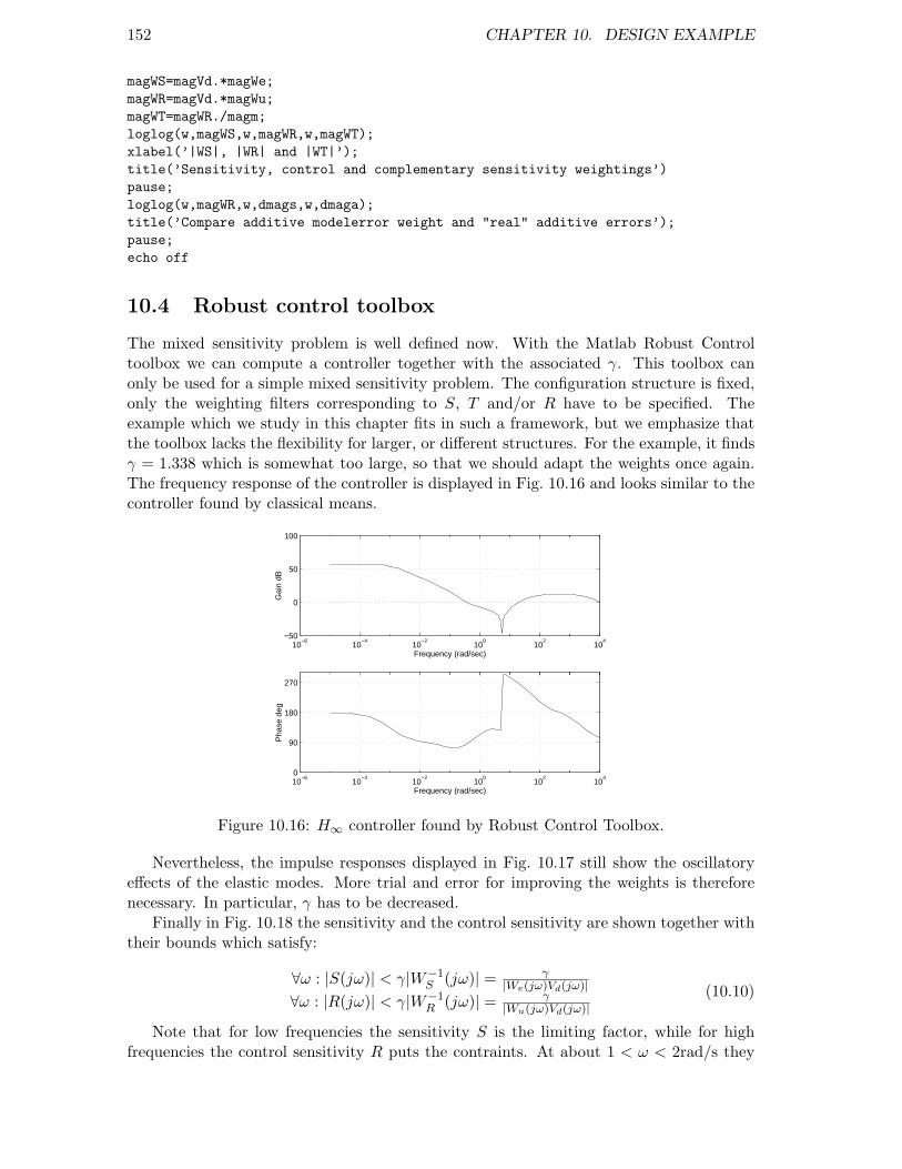
152 CHAPTER 10. DESIGN EXAMPLE
magWS=magVd.*magWe;magWR=magVd.*magWu;magWT=magWR./magm;loglog(w,magWS,w,magWR,w,magWT);xlabel(’|WS|, |WR| and |WT|’);title(’Sensitivity, control and complementary sensitivity weightings’)pause;loglog(w,magWR,w,dmags,w,dmaga);title(’Compare additive modelerror weight and "real" additive errors’);pause;echo off
10.4 Robust control toolbox
The mixed sensitivity problem is well defined now. With the Matlab Robust Controltoolbox we can compute a controller together with the associated γ. This toolbox canonly be used for a simple mixed sensitivity problem. The configuration structure is fixed,only the weighting filters corresponding to S, T and/or R have to be specified. Theexample which we study in this chapter fits in such a framework, but we emphasize thatthe toolbox lacks the flexibility for larger, or different structures. For the example, it findsγ = 1.338 which is somewhat too large, so that we should adapt the weights once again.The frequency response of the controller is displayed in Fig. 10.16 and looks similar to thecontroller found by classical means.
10−6
10−4
10−2
100
102
104
−50
0
50
100
Frequency (rad/sec)
Gai
n dB
10−6
10−4
10−2
100
102
104
0
90
180
270
Frequency (rad/sec)
Pha
se d
eg
Figure 10.16: H∞ controller found by Robust Control Toolbox.
Nevertheless, the impulse responses displayed in Fig. 10.17 still show the oscillatoryeffects of the elastic modes. More trial and error for improving the weights is thereforenecessary. In particular, γ has to be decreased.
Finally in Fig. 10.18 the sensitivity and the control sensitivity are shown together withtheir bounds which satisfy:
∀ω : |S(jω)| < γ|W−1S (jω)| = γ
|We(jω)Vd(jω)|∀ω : |R(jω)| < γ|W−1
R (jω)| = γ|Wu(jω)Vd(jω)|
(10.10)
Note that for low frequencies the sensitivity S is the limiting factor, while for highfrequencies the control sensitivity R puts the contraints. At about 1 < ω < 2rad/s they
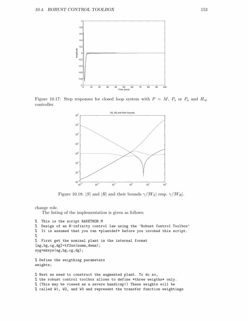
10.4. ROBUST CONTROL TOOLBOX 153
0 10 20 30 40 50 60 70 80 90 100−1
−0.8
−0.6
−0.4
−0.2
0
0.2
0.4
0.6
0.8
1
Time (secs)
Am
plitu
de
Figure 10.17: Step responses for closed loop system with P = M , Ps or Pa and H∞controller.
10−3
10−2
10−1
100
101
102
10−3
10−2
10−1
100
101
102
103
104
|S|, |R| and their bounds
Figure 10.18: |S| and |R| and their bounds γ/|WS | resp. γ/|WR|.
change role.The listing of the implementation is given as follows:
% This is the script RAKETROB.M% Design of an H-infinity control law using the ’Robust Control Toolbox’% It is assumed that you ran *plantdef* before you invoked this script.%% First get the nominal plant in the internal format[ag,bg,cg,dg]=tf2ss(numm,denm);syg=mksys(ag,bg,cg,dg);
% Define the weigthing parametersweights;
% Next we need to construct the augmented plant. To do so,% the robust control toolbox allows to define *three weigths* only.% (This may be viewed as a severe handicap!) These weights will be% called W1, W2, and W3 and represent the transfer function weightings

154 CHAPTER 10. DESIGN EXAMPLE
% on the controlled system sensitivity (S), control sensitivity (R)% and complementary sensitivity (T), respectively. From our configuration% we find that W1 = Vd*We, W2=Vd*Wu and W3 is not in use. We specify% this in state space form as follows.[aw1,bw1,cw1,dw1]=tf2ss(conv(numVd,numWe),conv(denVd,denWe));ssw1=mksys(aw1,bw1,cw1,dw1);[aw2,bw2,cw2,dw2]=tf2ss(conv(numVd,numWu),conv(denVd,denWu));ssw2=mksys(aw2,bw2,cw2,dw2);ssw3=mksys([],[],[],[]);
% the augmented system is now generated with the command *augss*% (sorry, it is the only command for this purpose in this toolbox...)[tss]=augss(syg,ssw1,ssw2,ssw3);
% Controller synthesis in this toolbox is done with the routine% *hinfopt*. Check out the help information on this routine and% find out that we actually compute 1/gamma where gamma is% the ‘usual’ gamma that we use throughout the lecture notes.[gamma,ssf,sscl]=hinfopt(tss,[1:2],[.001,1,0]);gamma=1/gamma;disp(’Optimal H-infinity norm is approximately ’);disp(num2str(gamma));
% Next we evaluate the robust performance of this controller[af,bf,cf,df]=branch(ssf); % returns the controller in state space formbode(af,bf,cf,df); pause;[as,bs,cs,ds]=tf2ss(nums,dens); % returns Ps in state space form[aa,ba,ca,da]=tf2ss(numa,dena); % returns Pa in state space form[alm,blm,clm,dlm]=series(af,bf,cf,df,ag,bg,cg,dg);[als,bls,cls,dls]=series(af,bf,cf,df,as,bs,cs,ds);[ala,bla,cla,dla]=series(af,bf,cf,df,aa,ba,ca,da);[acle,bcle,ccle,dcle]=feedback([],[],[],1,alm,blm,clm,dlm,-1);[aclu,bclu,cclu,dclu]=feedback(af,bf,cf,df,ag,bg,cg,dg,-1);[acls,bcls,ccls,dcls]=feedback([],[],[],1,als,bls,cls,dls,-1);[acla,bcla,ccla,dcla]=feedback([],[],[],1,ala,bla,cla,dla,-1);step(acle,bcle,ccle,dcle);hold;step(acls,bcls,ccls,dcls);step(acla,bcla,ccla,dcla);pause;hold off;boundR=gamma./magWR; boundS=gamma./magWS;magcle=bode(acle,bcle,ccle,dcle,1,w);magclu=bode(aclu,bclu,cclu,dclu,1,w);loglog(w,magcle,w,magclu,w,boundR,w,boundS);title(’|S|, |R| and their bounds’);
10.5 H∞ design in mutools.
In the “µ-analysis and synthesis toolbox”, simply indicated by “Mutools”, we have plentyof freedom to define the structure of the augmented plant ourselves. The listing for theexample under study raketmut.m is given as:
%% SCRIPT FILE FOR THE CALCULATION AND EVALUATION

10.5. H∞ DESIGN IN MUTOOLS. 155
% OF CONTROLLERS USING THE MU-TOOLBOX%% This script assumes that you ran the files plantdef and weights%
% REPRESENT SYSTEM BLOCKS IN INTERNAL FORMATPlant=nd2sys(numm,denm);Vd=nd2sys(numVd,denVd);We=nd2sys(numWe,denWe);Wu=nd2sys(numWu,denWu);
% MAKE GENERALIZED PLANT USING *sysic*systemnames=’Plant Vd We Wu’;inputvar=’[dw;u]’;outputvar=’[We;Wu;-Plant-Vd]’;input_to_Plant=’[u]’;input_to_Vd=’[dw]’;input_to_We=’[-Plant-Vd]’;input_to_Wu=’[u]’;sysoutname=’G’;cleanupsysic=’yes’;sysic;
% CALCULATE CONTROLLER[Contr,fclp,gamma]=hinfsyn(G,1,1,0,10,1e-4);
% MAKE CLOSED LOOP INTERCONNECTION FOR MODELsystemnames=’Contr Plant’;inputvar=’[d]’;outputvar=’[-Plant-d;Contr]’;input_to_Plant=’[Contr]’;input_to_Contr=’[-Plant-d]’;sysoutname=’realclp’;cleanupsysic=’yes’;sysic;
% MAKE CLOSED LOOP INTERCONNECTION FOR PsPlants=nd2sys(nums,dens);systemnames=’Contr Plants’;inputvar=’[d]’;outputvar=’[-Plants-d;Contr]’;input_to_Plants=’[Contr]’;input_to_Contr=’[-Plants-d]’;sysoutname=’realclps’;cleanupsysic=’yes’;sysic;
% MAKE CLOSED LOOP INTERCONNECTION FOR PaPlanta=nd2sys(numa,dena);systemnames=’Contr Planta’;inputvar=’[d]’;outputvar=’[-Planta-d;Contr]’;input_to_Planta=’[Contr]’;input_to_Contr=’[-Planta-d]’;sysoutname=’realclpa’;cleanupsysic=’yes’;
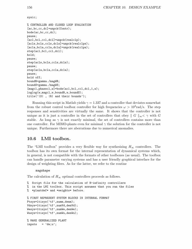
156 CHAPTER 10. DESIGN EXAMPLE
sysic;
% CONTROLLER AND CLOSED LOOP EVALUATION[ac,bc,cc,dc]=unpck(Contr);bode(ac,bc,cc,dc);pause;[acl,bcl,ccl,dcl]=unpck(realclp);[acls,bcls,ccls,dcls]=unpck(realclps);[acla,bcla,ccla,dcla]=unpck(realclpa);step(acl,bcl,ccl,dcl);hold;pause;step(acls,bcls,ccls,dcls);pause;step(acla,bcla,ccla,dcla);pause;hold off;boundR=gamma./magWR;boundS=gamma./magWS;[magcl,phasecl,w]=bode(acl,bcl,ccl,dcl,1,w);loglog(w,magcl,w,boundR,w,boundS);title(’|S| , |R| and their bounds’);
Running this script in Matlab yields γ = 1.337 and a controller that deviates somewhatfrom the robust control toolbox controller for high frequencies ω > 103rad/s. The stepresponses and sensitivities are virtually the same. It shows that the controller is notunique as it is just a controller in the set of controllers that obey ‖ G ‖∞< γ with Gstable. As long as γ is not exactly minimal, the set of controllers contains more thanone controller. For MIMO-plants even for minimal γ the solution for the controller is notunique. Furthermore there are aberrations due to numerical anomalies.
10.6 LMI toolbox.
The “LMI toolbox” provides a very flexible way for synthesizing H∞ controllers. Thetoolbox has its own format for the internal representation of dynamical systems which,in general, is not compatible with the formats of other toolboxes (as usual). The toolboxcan handle parameter varying systems and has a user friendly graphical interface for thedesign of weighting filers. As for the latter, we refer to the routine
magshape
The calculation of H∞ optimal controllers proceeds as follows.
% Script file for the calculation of H-infinity controllers% in the LMI toolbox. This script assumes that you ran the files% *plantdef* and *weights* before.
% FIRST REPRESENT SYSTEM BLOCKS IN INTERNAL FORMATPtsys=ltisys(’tf’,numm,denm);Vdsys=ltisys(’tf’,numVd,denVd);Wesys=ltisys(’tf’,numWe,denWe);Wusys=ltisys(’tf’,numWu,denWu);
% MAKE GENERALIZED PLANTinputs = ’dw;u’;

10.7. µ DESIGN IN MUTOOLS 157
outputs = ’We;Wu;-Pt-Vd’;Ptin=’Pt : u’;Vdin=’Vd : dw’;Wein=’We : -Pt-Vd’;Wuin=’Wu : u’;G=sconnect(inputs,outputs,[],Ptin,Ptsys,Vdin,Vdsys,...Wein,Wesys,Wuin,Wusys);
% CALCULATE H-INFTY CONTROLLER USING LMI SOLUTION[gamma,Ksys]=hinflmi(G,[1 1],0,1e-4);
% MAKE CLOSED-LOOP INTERCONNECTION FOR MODELSsys = sinv(sadd(1,smult(Ptsys,Ksys)));Rsys = smult(Ksys,Ssys);
% EVALUATE CONTROLLED SYSTEMsplot(Ksys,’bo’,w); title(’Bodeplot of controller’);pausesplot(Ssys,’sv’); title(’Maximal singular value of Sensitivity’);pausesplot(Ssys,’ny’); title(’Nyquist plot of Sensitivity’)pausesplot(Ssys,’st’); title(’Step response of Sensitivity’);pausesplot(Rsys,’sv’); title(’Maximal sv of Control Sensitivity’);pausesplot(Rsys,’ny’); title(’Nyquist plot of Control Sensitivity’);pausesplot(Rsys,’st’); title(’Step response of Control Sensitivity’);pause
10.7 µ design in mutools
In µ-design we pretend to model the variability of the flexible mode very tightly by meansof specific parameters in stead of the rough modelling by an additive perturbation boundby WuVd. In that way we hope to obtain a less conservative controller. We suppose thatthe poles and zeros of the flexible mode shift along a straight line in complex plane betweenthe extreme positions of Ps and Pa as illustrated in Fig. 10.19.
6j
5j
−.06 −.05
Figure 10.19: Variability of elastic mode.

158 CHAPTER 10. DESIGN EXAMPLE
Algebraically this variation can then be represented by one parameter δ according to:
∀ δεR,−1 ≤ δ ≤ 1poles : −.055− .005δ ± j(5.5 + .5δ)zeros : −.055 + .005δ ± j(5.5− .5δ)
(10.11)
So that the total transfer of the plant including the perturbation is given by:
Pt(s) =−8(s+ .125)(s− 1)(s+ 1)
∗ (10.12)
K0(s+ .055− .005δ − j(5.5− .5δ))(s+ .055− .005δ + j(5.5− .5δ))(s+ .055 + .005δ − j(5.5 + .5δ))(s+ .055 + .005δ + j(5.5 + .5δ))
(10.13)
where the extra constant K0 is determined by Pt(0) = 1: the DC-gain is kept on 1.If we define the nominal position of the poles and zeros by a0 = .055 and b0 = 5.5
rearrangement yields:
Pt(s) = −8s+ .125s2 − 1
∗ 1 + ∆mult (10.14)
∆mult = k0−δ(.02s+ .02a0 + 2b0)
s2 + (2a0 + .01δ)s+ a20 + b20 + δ(.01a0 + b0) + .250025δ2
(10.15)
k0 =a2
0 + b20 + .250025δ2 + δ(.01a0 + b0)a2
0 + b20 + .250025δ2 − δ(.01a0 + b0)(10.16)
The factor F = 1 + ∆mult can easily be brought into a state space description withA,B,C,D:
A = A1 + dA =(
0 1−a2
0 − b20 −2a0
)+(
0 0−γδ − εδ2 .01δ
)C = C1 + dC =
(0 0
)+ a2
0+b20+γδ+εδ2
a20+b20−γδ+εδ2
( −αδ −.02δ)
B = B1 + dB =(
01
)+(
00
)D = D1 + dD = 1 + 0 α = 11.0011; γ = 5.50055; ε = .250025
(10.17)
Note that for δ = 0 we simply have F = 1 + ∆mult = 1.If we let δ = δ(s) with |δ(jω)| ≤ 1 we have given the parameter delta much more
freedom, but the whole description then fits with the µ-analysis. We have for the dynamictransfer F (s):
sx = A1x+B1u1 + dA(s)x+ dB(s)u1 dB(s) = 0y1 = C1x+D1u1 + dC(s)x+ dD(s)u1 dD(s) = 0
(10.18)
With β = a20 + b20 = 30.2502 we rewrite:
dA =(
0 0−γδ − εδ2 −.02δ
)dC =
(−αδ
(1 + α
β−γδ+εδ2
)0)
(10.19)
Next we can define 5 extra input lines in a vector u2 and correspondingly 5 extraoutput lines in a vector y2 that are linked in a closed loop via u2 = ∆y2 with:
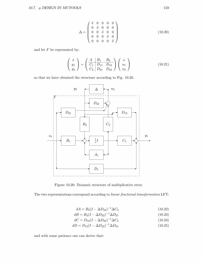
10.7. µ DESIGN IN MUTOOLS 159
∆ =
δ 0 0 0 00 δ 0 0 00 0 δ 0 00 0 0 δ 00 0 0 0 δ
(10.20)
and let F be represented by:
xy1y2
=
A B1 B2
C1 D11 D12C2 D21 D22
xu1u2
(10.21)
so that we have obtained the structure according to Fig. 10.20.
D1
A1
1sI
C2B2
D22
D12D21
B1 C1
∆
u1 y1
u2y2
F
Figure 10.20: Dynamic structure of multiplicative error.
The two representations correspond according to linear fractional transformation LFT:
dA = B2(I −∆D22)−1∆C2 (10.22)dB = B2(I −∆D22)−1∆D21 (10.23)dC = D12(I −∆D22)−1∆C2 (10.24)dD = D12(I −∆D22)−1∆D21 (10.25)
and with some patience one can derive that:
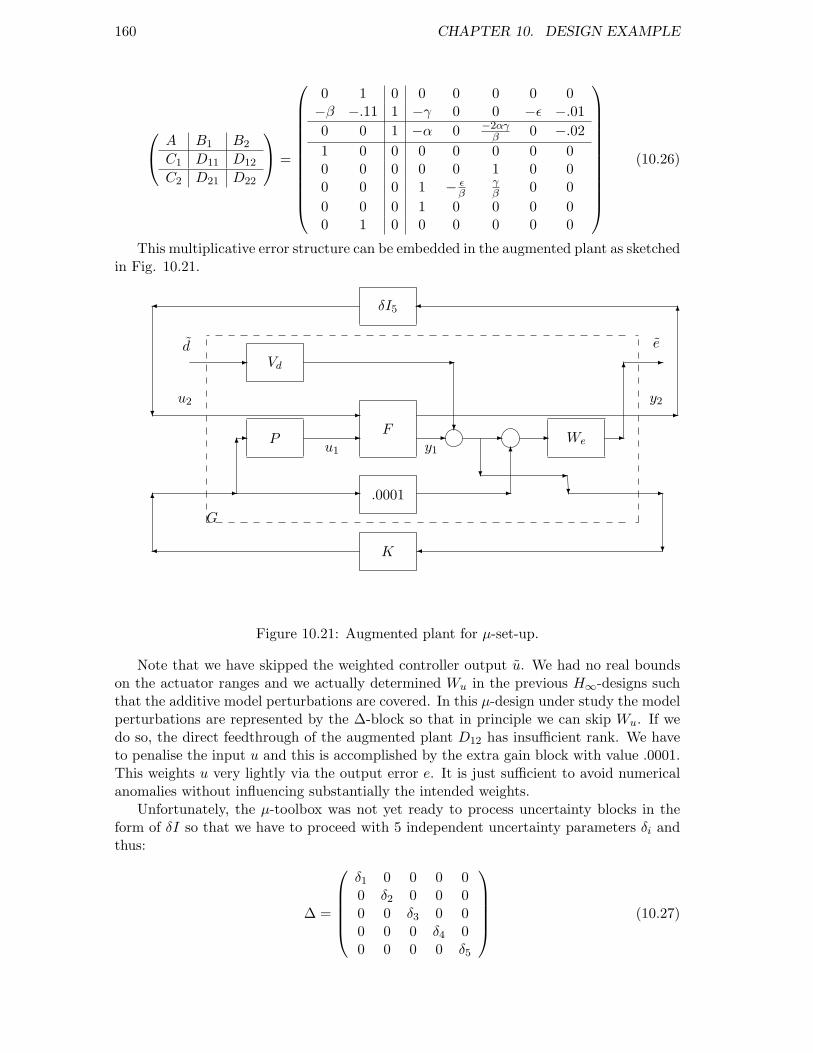
160 CHAPTER 10. DESIGN EXAMPLE
A B1 B2
C1 D11 D12
C2 D21 D22
=
0 1 0 0 0 0 0 0−β −.11 1 −γ 0 0 −ε −.010 0 1 −α 0 −2αγ
β 0 −.021 0 0 0 0 0 0 00 0 0 0 0 1 0 00 0 0 1 − ε
βγβ 0 0
0 0 0 1 0 0 0 00 1 0 0 0 0 0 0
(10.26)
This multiplicative error structure can be embedded in the augmented plant as sketchedin Fig. 10.21.
K
.0001
FP
Vd
We
G
δI5
d
u2
e
y2
u1 y1
Figure 10.21: Augmented plant for µ-set-up.
Note that we have skipped the weighted controller output u. We had no real boundson the actuator ranges and we actually determined Wu in the previous H∞-designs suchthat the additive model perturbations are covered. In this µ-design under study the modelperturbations are represented by the ∆-block so that in principle we can skip Wu. If wedo so, the direct feedthrough of the augmented plant D12 has insufficient rank. We haveto penalise the input u and this is accomplished by the extra gain block with value .0001.This weights u very lightly via the output error e. It is just sufficient to avoid numericalanomalies without influencing substantially the intended weights.
Unfortunately, the µ-toolbox was not yet ready to process uncertainty blocks in theform of δI so that we have to proceed with 5 independent uncertainty parameters δi andthus:
∆ =
δ1 0 0 0 00 δ2 0 0 00 0 δ3 0 00 0 0 δ4 00 0 0 0 δ5
(10.27)

10.7. µ DESIGN IN MUTOOLS 161
As a consequence the design will be more conservative, but the controller will becomemore robust. The commands for solving this design in the µ-toolbox are given in the nextscript:
% Let’s make the system DMULT firstalpha=11.0011; beta=30.25302;gamma=5.50055; epsilon=.250025;ADMULT=[0,1;-beta,-.11];BDMULT=[0,0,0,0,0,0;1,-gamma,0,0,-epsilon,-.01];CDMULT=[0,0,;1,0;0,0;0,0;0,0;0,1];DDMULT=[1,-alpha,0,-2*alpha*gamma/beta,0,-.02; ...
0,0,0,0,0,0; ...0,0,0,1,0,0; ...0,1,-epsilon/beta,gamma/beta,0,0,; ...0,1,0,0,0,0; ...0,0,0,0,0,0];
mat=[ADMULT BDMULT;CDMULT DDMULT];DMULT=pss2sys(mat,2);
% MAKE GENERALIZED MUPLANTsystemnames=’Plant Vd We DMULT’;inputvar=’[u2(5);dw;x]’;outputvar=’[DMULT(2:6);We+.0001*x;-DMULT(1)-Vd]’;input_to_Plant=’[x]’;input_to_Vd=’[dw]’;input_to_We=’[-DMULT(1)-Vd]’;input_to_DMULT=’[Plant;u2(1:5)]’;sysoutname=’GMU’;cleanupsysic=’yes’;sysic;
% CALCULATE HINF CONTROLLER
[k1,clp1]=hinfsyn(GMU,1,1,0,100,1e-4);
% PROPERTIES OF CONTROLLER
omega=logspace(-2,3,100);spoles(k1)k1_g=frsp(k1,omega);vplot(’bode’,k1_g);pause;clp1_g=frsp(clp1,omega);blk=[1 1;1 1; 1 1;1 1;1 1];blkp=[1 1;1 1;1 1;1 1;1 1;1 1];[bnds1,dvec1,sens1,pvec1]=mu(clp1_g,blkp);vplot(’liv,m’,vnorm(clp1_g),bnds1);pause;
% FIRST mu-CONTROLLER
[dsysL1,dsysR1]=musynfit(’first’,dvec1,sens1,blkp,1,1);mu_inc1=mmult(dsysL1,GMU,minv(dsysR1));[k2,clp2]=hinfsyn(mu_inc1,1,1,0,100,1e-4);clp2_g=frsp(clp2,omega);[bnds2,dvec2,sens2,pvec2]=mu(clp2_g,blkp);

162 CHAPTER 10. DESIGN EXAMPLE
vplot(’liv,m’,vnorm(clp2_g),bnds2);pause[ac,bc,cc,dc]=unpck(k2);bode(ac,bc,cc,dc);pause;
% MAKE CLOSED LOOP INTERCONNECTION FOR MODELsystemnames=’k2 Plant’;inputvar=’[d]’;outputvar=’[-Plant-d;k2]’;input_to_Plant=’[k2]’;input_to_k2=’[-Plant-d]’;sysoutname=’realclp’;cleanupsysic=’yes’;sysic;
% MAKE CLOSED LOOP INTERCONNECTION FOR PsPlants=nd2sys(nums,dens);systemnames=’k2 Plants’;inputvar=’[d]’;outputvar=’[-Plants-d;k2]’;input_to_Plants=’[k2]’;input_to_k2=’[-Plants-d]’;sysoutname=’realclps’;cleanupsysic=’yes’;sysic;
% MAKE CLOSED LOOP INTERCONNECTION FOR PaPlanta=nd2sys(numa,dena);systemnames=’k2 Planta’;inputvar=’[d]’;outputvar=’[-Planta-d;k2]’;input_to_Planta=’[k2]’;input_to_k2=’[-Planta-d]’;sysoutname=’realclpa’;cleanupsysic=’yes’;sysic;
% Controller and closed loop evaluation
[acl,bcl,ccl,dcl]=unpck(realclp);[acls,bcls,ccls,dcls]=unpck(realclps);[acla,bcla,ccla,dcla]=unpck(realclpa);step(acl,bcl,ccl,dcl);hold;pause;step(acls,bcls,ccls,dcls);pause;step(acla,bcla,ccla,dcla);pause;hold off;
% SECOND mu-CONTROLLERspoles(k2)k2_g=frsp(k2,omega);vplot(’bode’,k2_g);

10.7. µ DESIGN IN MUTOOLS 163
pause;
[dsysL2,dsysR2]=musynfit(dsysL1,dvec2,sens2,blkp,1,1);mu_inc2=mmult(dsysL2,mu_inc1,minv(dsysR2));[k3,clp3]=hinfsyn(mu_inc2,1,1,0,100,1e-4);clp3_g=frsp(clp3,omega);[bnds3,dvec3,sens3,pvec3]=mu(clp3_g,blkp);vplot(’liv,m’,vnorm(clp3_g),bnds3);pause[ac,bc,cc,dc]=unpck(k3);bode(ac,bc,cc,dc);pause;
% MAKE CLOSED LOOP INTERCONNECTION FOR MODELsystemnames=’k3 Plant’;inputvar=’[d]’;outputvar=’[-Plant-d;k3]’;input_to_Plant=’[k3]’;input_to_k3=’[-Plant-d]’;sysoutname=’realclp’;cleanupsysic=’yes’;sysic;
% MAKE CLOSED LOOP INTERCONNECTION FOR PsPlants=nd2sys(nums,dens);systemnames=’k3 Plants’;inputvar=’[d]’;outputvar=’[-Plants-d;k3]’;input_to_Plants=’[k3]’;input_to_k3=’[-Plants-d]’;sysoutname=’realclps’;cleanupsysic=’yes’;sysic;
% MAKE CLOSED LOOP INTERCONNECTION FOR PaPlanta=nd2sys(numa,dena);systemnames=’k3 Planta’;inputvar=’[d]’;outputvar=’[-Planta-d;k3]’;input_to_Planta=’[k3]’;input_to_k3=’[-Planta-d]’;sysoutname=’realclpa’;cleanupsysic=’yes’;sysic;
% Controller and closed loop evaluation
[acl,bcl,ccl,dcl]=unpck(realclp);[acls,bcls,ccls,dcls]=unpck(realclps);[acla,bcla,ccla,dcla]=unpck(realclpa);step(acl,bcl,ccl,dcl);hold;pause;step(acls,bcls,ccls,dcls);pause;step(acla,bcla,ccla,dcla);

164 CHAPTER 10. DESIGN EXAMPLE
pause;hold off;
First the H∞-controller for the augmented plant is computed. The γ = 33.0406,much too high. Next one is invited to choose the respective orders of the filters thatapproximate the D-scalings for a number of frequencies. If one chooses a zero order, thefirst approximate µ = γ = 19.9840 and yields un Pa unstable at closed loop. A seconditeration with second order approximate filters even increases µ = γ = 29.4670 and Pa
remains unstable.A second try with second order filters in the first iteration brings µ = γ down to 5.4538
but still leads to an unstable Pa. In second iteration with second order filters the programfails altogether.
Stimulated nevertheless by the last attempt we increase the first iteration order to 3which produces a µ = γ = 4.9184 and a Pa that just oscillates in feedback. A seconditeration with first order filters increases the µ = γ to 21.2902, but the resulting closedloops are all stable.
Going still higher we take both iterations with 4-th order filters and the µ = γ take therespective values 4.4876 and 10.8217. In the first iteration the Pa still shows a ill dampedoscillation, but the second iteration results in very stable closed loops for all P , Ps andPa. The cost is a very complicated controller of the order 4+10*4+10*4=44!
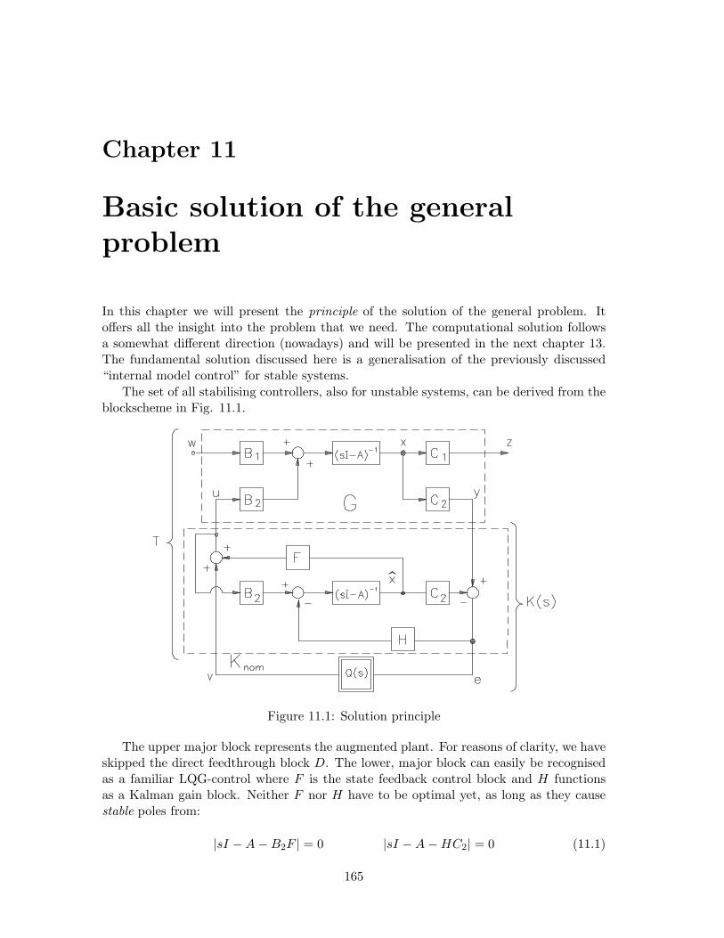
Chapter 11
Basic solution of the generalproblem
In this chapter we will present the principle of the solution of the general problem. Itoffers all the insight into the problem that we need. The computational solution followsa somewhat different direction (nowadays) and will be presented in the next chapter 13.The fundamental solution discussed here is a generalisation of the previously discussed“internal model control” for stable systems.
The set of all stabilising controllers, also for unstable systems, can be derived from theblockscheme in Fig. 11.1.
Figure 11.1: Solution principle
The upper major block represents the augmented plant. For reasons of clarity, we haveskipped the direct feedthrough block D. The lower, major block can easily be recognisedas a familiar LQG-control where F is the state feedback control block and H functionsas a Kalman gain block. Neither F nor H have to be optimal yet, as long as they causestable poles from:
|sI −A−B2F | = 0 |sI −A−HC2| = 0 (11.1)
165
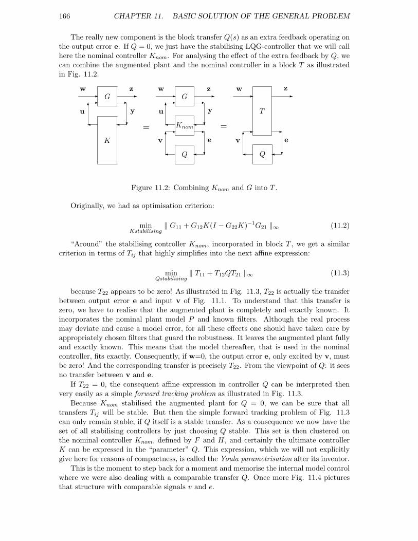
166 CHAPTER 11. BASIC SOLUTION OF THE GENERAL PROBLEM
The really new component is the block transfer Q(s) as an extra feedback operating onthe output error e. If Q = 0, we just have the stabilising LQG-controller that we will callhere the nominal controller Knom. For analysing the effect of the extra feedback by Q, wecan combine the augmented plant and the nominal controller in a block T as illustratedin Fig. 11.2.
Q Q
Knom
K
GG
T
w z w z w z
u y u y
v e v e
= =
Figure 11.2: Combining Knom and G into T .
Originally, we had as optimisation criterion:
minKstabilising
‖ G11 +G12K(I −G22K)−1G21 ‖∞ (11.2)
“Around” the stabilising controller Knom, incorporated in block T , we get a similarcriterion in terms of Tij that highly simplifies into the next affine expression:
minQstabilising
‖ T11 + T12QT21 ‖∞ (11.3)
because T22 appears to be zero! As illustrated in Fig. 11.3, T22 is actually the transferbetween output error e and input v of Fig. 11.1. To understand that this transfer iszero, we have to realise that the augmented plant is completely and exactly known. Itincorporates the nominal plant model P and known filters. Although the real processmay deviate and cause a model error, for all these effects one should have taken care byappropriately chosen filters that guard the robustness. It leaves the augmented plant fullyand exactly known. This means that the model thereafter, that is used in the nominalcontroller, fits exactly. Consequently, if w=0, the output error e, only excited by v, mustbe zero! And the corresponding transfer is precisely T22. From the viewpoint of Q: it seesno transfer between v and e.
If T22 = 0, the consequent affine expression in controller Q can be interpreted thenvery easily as a simple forward tracking problem as illustrated in Fig. 11.3.
Because Knom stabilised the augmented plant for Q = 0, we can be sure that alltransfers Tij will be stable. But then the simple forward tracking problem of Fig. 11.3can only remain stable, if Q itself is a stable transfer. As a consequence we now have theset of all stabilising controllers by just choosing Q stable. This set is then clustered onthe nominal controller Knom, defined by F and H, and certainly the ultimate controllerK can be expressed in the “parameter” Q. This expression, which we will not explicitlygive here for reasons of compactness, is called the Youla parametrisation after its inventor.
This is the moment to step back for a moment and memorise the internal model controlwhere we were also dealing with a comparable transfer Q. Once more Fig. 11.4 picturesthat structure with comparable signals v and e.
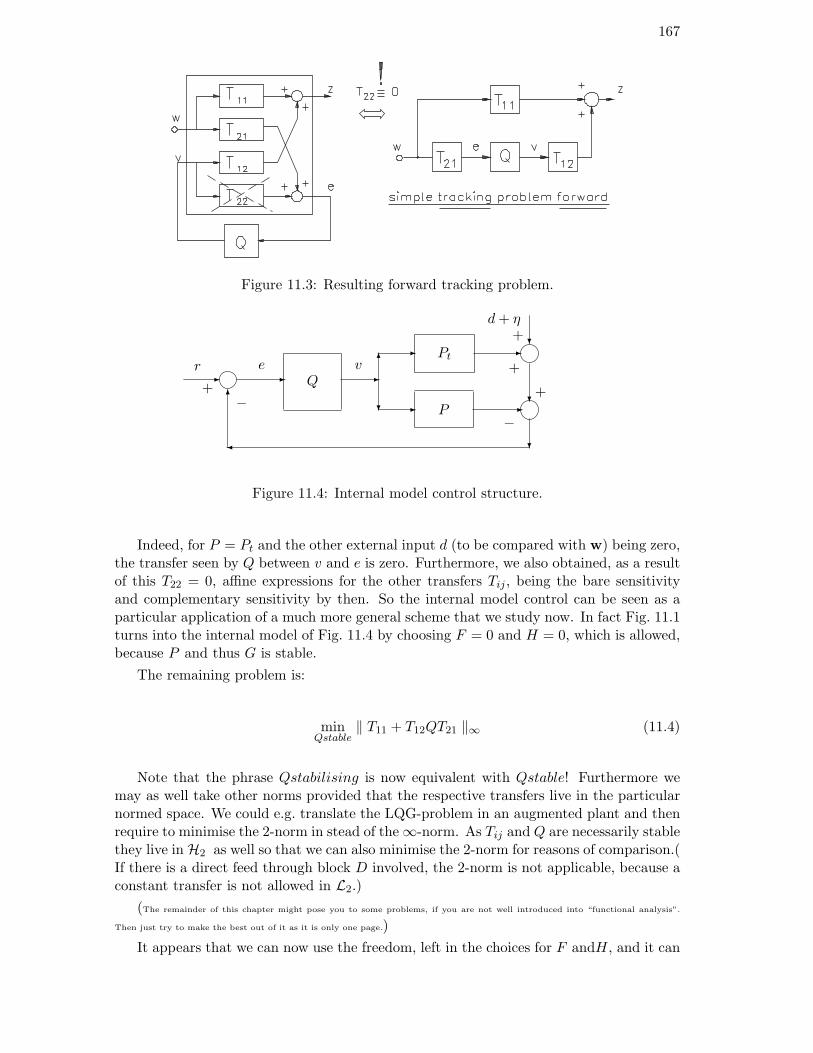
167
Figure 11.3: Resulting forward tracking problem.
P
Pt
Q
r
+−
e v
+
+
+
−
d+ η
Figure 11.4: Internal model control structure.
Indeed, for P = Pt and the other external input d (to be compared with w) being zero,the transfer seen by Q between v and e is zero. Furthermore, we also obtained, as a resultof this T22 = 0, affine expressions for the other transfers Tij , being the bare sensitivityand complementary sensitivity by then. So the internal model control can be seen as aparticular application of a much more general scheme that we study now. In fact Fig. 11.1turns into the internal model of Fig. 11.4 by choosing F = 0 and H = 0, which is allowed,because P and thus G is stable.
The remaining problem is:
minQstable
‖ T11 + T12QT21 ‖∞ (11.4)
Note that the phrase Qstabilising is now equivalent with Qstable! Furthermore wemay as well take other norms provided that the respective transfers live in the particularnormed space. We could e.g. translate the LQG-problem in an augmented plant and thenrequire to minimise the 2-norm in stead of the∞-norm. As Tij and Q are necessarily stablethey live in H2 as well so that we can also minimise the 2-norm for reasons of comparison.(If there is a direct feed through block D involved, the 2-norm is not applicable, because aconstant transfer is not allowed in L2.)
(The remainder of this chapter might pose you to some problems, if you are not well introduced into “functional analysis”.
Then just try to make the best out of it as it is only one page.)It appears that we can now use the freedom, left in the choices for F andH, and it can
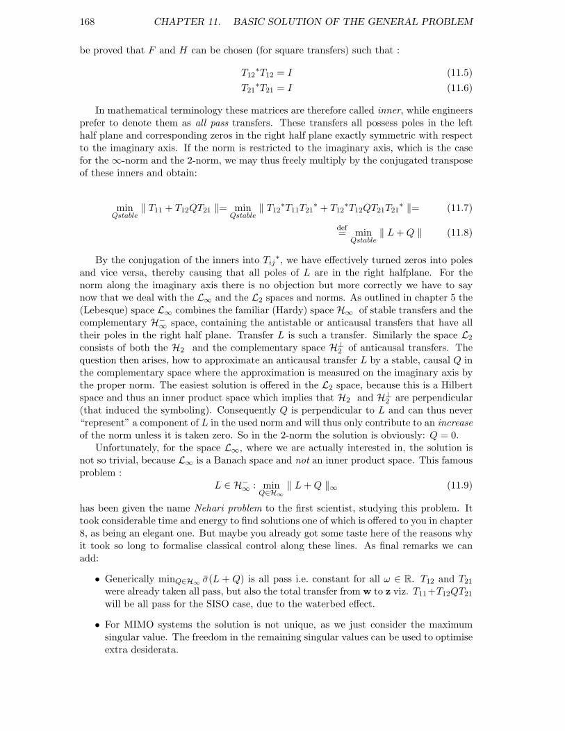
168 CHAPTER 11. BASIC SOLUTION OF THE GENERAL PROBLEM
be proved that F and H can be chosen (for square transfers) such that :
T12∗T12 = I (11.5)
T21∗T21 = I (11.6)
In mathematical terminology these matrices are therefore called inner, while engineersprefer to denote them as all pass transfers. These transfers all possess poles in the lefthalf plane and corresponding zeros in the right half plane exactly symmetric with respectto the imaginary axis. If the norm is restricted to the imaginary axis, which is the casefor the∞-norm and the 2-norm, we may thus freely multiply by the conjugated transposeof these inners and obtain:
minQstable
‖ T11 + T12QT21 ‖= minQstable
‖ T12∗T11T21
∗ + T12∗T12QT21T21
∗ ‖= (11.7)
def= minQstable
‖ L+Q ‖ (11.8)
By the conjugation of the inners into Tij∗, we have effectively turned zeros into poles
and vice versa, thereby causing that all poles of L are in the right halfplane. For thenorm along the imaginary axis there is no objection but more correctly we have to saynow that we deal with the L∞ and the L2 spaces and norms. As outlined in chapter 5 the(Lebesque) space L∞ combines the familiar (Hardy) space H∞ of stable transfers and thecomplementary H−∞ space, containing the antistable or anticausal transfers that have alltheir poles in the right half plane. Transfer L is such a transfer. Similarly the space L2consists of both the H2 and the complementary space H⊥
2 of anticausal transfers. Thequestion then arises, how to approximate an anticausal transfer L by a stable, causal Q inthe complementary space where the approximation is measured on the imaginary axis bythe proper norm. The easiest solution is offered in the L2 space, because this is a Hilbertspace and thus an inner product space which implies that H2 and H⊥
2 are perpendicular(that induced the symboling). Consequently Q is perpendicular to L and can thus never“represent” a component of L in the used norm and will thus only contribute to an increaseof the norm unless it is taken zero. So in the 2-norm the solution is obviously: Q = 0.
Unfortunately, for the space L∞, where we are actually interested in, the solution isnot so trivial, because L∞ is a Banach space and not an inner product space. This famousproblem :
L ∈ H−∞ : min
Q∈H∞‖ L+Q ‖∞ (11.9)
has been given the name Nehari problem to the first scientist, studying this problem. Ittook considerable time and energy to find solutions one of which is offered to you in chapter8, as being an elegant one. But maybe you already got some taste here of the reasons whyit took so long to formalise classical control along these lines. As final remarks we canadd:
• Generically minQ∈H∞ σ(L + Q) is all pass i.e. constant for all ω ∈ R. T12 and T21were already taken all pass, but also the total transfer from w to z viz. T11+T12QT21will be all pass for the SISO case, due to the waterbed effect.
• For MIMO systems the solution is not unique, as we just consider the maximumsingular value. The freedom in the remaining singular values can be used to optimiseextra desiderata.

11.1. EXERCISES 169
11.1 Exercises
7.1:Consider the following feedback system:
• Plant: y = P (u+ d)
• Controller: u = K(r − y)• Errors: e1 = W1u and e2 = W2(r − y)
It is known that ‖ r ‖2≤ 1 and ‖ d ‖2≤ 1, and it is desired to design K so as to minimise:
‖ e1e2‖2
a) Show that this can be formulated as a standard H∞problem and compute G.
b) If P is stable, redefine the problem affine in Q.
7.2: Take the first blockscheme of the exercise of chapter 6. To facilitate the computa-tions we just consider a SISO-plant and DC-signals (i.e. only for ω = 0!) so that we avoidcomplex computations due to frequency dependence. If there is given that ‖ ξ ‖2< 1 andP = 1/2 then it is asked to minimise ‖ y ‖2 under the condition ‖ x ‖2< 1 while ξ is theonly input.
a) Solve this problem by means of a mixed sensitivity problem iteratively adapting Wy
renamed as β. Hint: First define V andWx. Sketch the solution in terms of controllerC and compute the solution directly as a function of β.
b) Solve the problem exactly: minimise ‖ y ‖2 while ‖ x ‖2< 1. Why is there a differencewith the solution sub a) ? Hint: For this question it is easier to define the problemaffine in Q.

170 CHAPTER 11. BASIC SOLUTION OF THE GENERAL PROBLEM
Chapter 12
Solution to the general H∞ controlproblem
12.1 Introduction
In previous chapters we have been mainly concerned with properties of control configura-tions in which a controller is designed so as to minimize the H∞ norm of a closed looptransfer function. So far, we did not address the question how such a controller is actuallycomputed. This has been a problem of main concern in the early 80-s. Various mathemat-ical techniques have been developed to compute ‘H∞-optimal controllers’, i.e., feedbackcontrollers which stabilize a closed loop system and at the same time minimize the H∞norm of a closed loop transfer function. In this chapter we treat a solution to a mostgeneral version of the H∞ optimal control problem which is now generally accepted tobe the fastest, simplest, and computationally most reliable and efficient way to synthesizeH∞ optimal controllers.
The solution which we present here is the result of almost a decenium of impressiveresearch effort in the area of H∞ optimal control and has received widespread attentionin the control community. An amazing number of scientific papers have appeared (andstill appear!) in this area of research. In this chapter we will treat a solution of thegeneral H∞ control problem which popularly is referred to as the ‘DGKF-solution’, theacronym standing for Doyle, Glover, Khargonekar and Francis, four authors of a famousand prize winning paper in the IEEE Transactions on Automatic Control1. From a math-ematical and system theoretic point of view, this so called ‘state space solution’ to theH∞ control problem is extremely elegant and worth a thorough treatment. However, forpractical applications it is sufficient to know the precise conditions under which the statespace solution ‘works’ so as to have a computationally reliable way to obtain and to de-sign H∞ optimal controllers. The solution presented in this chapter admits a relativelystraightforward implementation in a software environment like Matlab. The Robust Con-trol Toolbox has various routines for the synthesis of H∞ optimal controllers and we willdevote a section in this chapter on how to use these routines.
This chapter is organized as follows. In the next section we first treat the problemof how to compute the H2 norm and the H∞ norm of a transfer function. These resultswill be used in subsequent sections, where we present the main results concerning H∞controller synthesis in Theorem 12.7. We will make a comparison to the H2 optimal
1“State Space Solutions to the Standard H2 and H∞ Control Problems”, by J. Doyle, K. Glover, P.Khargonekar and B. Francis, IEEE Transactions on Automatic Control, August 1989.
171
172 CHAPTER 12. SOLUTION TO THE GENERAL H∞ CONTROL PROBLEM
control algorithms, which we briefly describe in a separate section and which you areprobably familiar with.
12.2 The computation of system norms
We start this chapter by considering the problem of characterizing the H2 and H∞ normsof a given (multivariable) transfer function H(s) in terms of a state space description ofthe system. We will consider the continuous time case only for the discrete time versionsof the results below are less insightfull and more involved.
Let H(s) be a stable transfer function of dimension p×m and suppose that
H(s) = C(Is−A)−1B +D
where A,B,C and D are real matrices defining the state space equations
x(t) = Ax(t) +Bw(t)z(t) = Cx(t) +Dw(t).
(12.1)
Since H(s) is stable, all eigenvalues of A are assumed to be in the left half complex plane.We suppose that the state space has dimension n and, to avoid redundancy, we moreoverassume that (12.1) defines a minimal state space representation of H(s) in the sense thatn is as small as possible among all state space representations of H(s).
Let us recall the definitions of the H2 and H∞ norms of H(s):
‖ H(s) ‖22 := 1/2π∫ ∞
−∞trace(H(jω)H∗(jω))dω
‖ H(s) ‖∞ := supω∈R
σ(H(jω))
where σ denotes the maximal singular value.
12.2.1 The computation of the H2 norm
We have seen in Chapter 5 that the (squared) H2 norm of a system has the simple inter-pretation as the sum of the (squared) L2 norms of the impulse responses which we canextract from (12.1). If we assume that D = 0 in (12.1) (otherwise the H2 norm is infiniteso H /∈ H2) and if bi denotes the i-th column of B, then the i-th impulse response is givenby
zi(t) = CeAtbi.
Since H(s) has m inputs, we have m of such responses, and for i = 1, . . . ,m, their L2norms satisfy
‖ zi ‖22 =∫ ∞
0bTi e
ATtCTCeAtbidt
= bTi
∫ ∞
0eA
TtCTCeAtdtbi
= bTi Mbi.
Here, we defined
M :=∫ ∞
0eA
TtCTCeAtdt
12.2. THE COMPUTATION OF SYSTEM NORMS 173
which is a square symmetric matrix of dimension n × n which is called the observabilitygramian of the system (12.1). Since xTMx ≥ 0 for all x ∈ Rn we have that M is non-negative definite2. In fact, the observability gramian M satisfies the equation
MA+ATM + CTC = 0 (12.2)
which is called a Lyapunov equation in the unknown M . Since we assumed that the statespace parameters (A,B,C,D) define a minimal representation of the transfer functionH(s), the pair (A,C) is observable3, and the matrix M is the only symmetric non-negativedefinite solution of (12.2). Thus, M can be computed from an algebraic equation, theLyapunov equation (12.2), which is a much simpler task than solving the infinite integralexpression for M .
The observability gramian M completely determines the H2 norm of the system H(s)as is seen from the following characterization.
Theorem 12.1 Let H(s) be a stable transfer function of the system described by thestate space equations (12.1). Suppose that (A,B,C,D) is a minimal representation ofH(s). Then
1. ‖ H(s) ‖2 < ∞ if and only if D = 0.
2. If M is the observability gramian of (12.1) then
‖ H(s) ‖22= trace(BTMB) =m∑
i=1
bTi Mbi.
Thus the H2 norm of H(s) is given by a trace formula involving the state space matricesA,B,C, from which the observability gramian M is computed. The main issue here isthat Theorem 12.1 provides an algebraic characterization of the H2 norm which provesextremely useful for computational purposes.
There is a ‘dual’ version of theorem 12.1 which is obtained from the fact that ‖H(s) ‖2=‖ H∗(s) ‖2. We state it for completeness
Theorem 12.2 Under the same conditions as in theorem 12.1,
‖ H(s) ‖22= trace(CWCT)
where W is the unique symmetric non-negative definite solution of the Lyapunov equation
AW +WAT +BBT = 0. (12.3)
The square symmetric matrix W is called the controllability gramian of the system (12.1).Theorem 12.2 therefore states that theH2 norm ofH(s) can also be obtained by computingthe controllability gramian associated with the system (12.1).
2which is not the same as saying that all elements of M are non-negative!!!3that is, CeAtx0 = 0 for all t ≥ 0 only if the initial condition x0 = 0.
174 CHAPTER 12. SOLUTION TO THE GENERAL H∞ CONTROL PROBLEM
12.2.2 The computation of the H∞ norm
The computation of the H∞ norm of a transfer function H(s) is slightly more involved.We will again present an algebraic algorithm, but instead of finding an exact expressionfor ‖ H(s) ‖∞, we will find an algebraic condition whether or not
‖ H(s) ‖∞ < γ (12.4)
for some real number γ ≥ 0. Thus, we will set up a test so as to determine whether (12.4)holds for certain value of γ ≥ 0. By performing this test for various values of γ we mayget arbitrarily close to the norm ‖ H(s) ‖∞.
We will briefly outline the main ideas behind this test. Recall from Chapter 5, thatthe H∞ norm is equal to the L2 induced norm of the transfer function, i.e.,
‖ H(s) ‖∞ = supw∈L2
‖ Hw ‖2‖ w ‖2 .
This means that ‖ H(s) ‖∞≤ γ if and only if
‖ Hw ‖22 −γ2 ‖ w ‖22=‖ z ‖22 −γ2 ‖ w ‖2 ≤ 0. (12.5)
for all w ∈ L2. (Indeed, dividing (12.5) by ‖ w ‖22 gives you the equivalence). Here,z = Hw is the output of the system (12.1) when the input w is applied and when theinitial state x(0) is set to 0.
Now, suppose that γ ≥ 0 and the system (12.1) is given. Motivated by the middleexpression of (12.5) we introduce for arbitrary initial conditions x(0) = x0 and any w ∈ L2,the criterion
J(x0, w) :=‖ z ‖22 −γ2 ‖ w ‖22=∫ ∞
0
(|z(t)|2 − γ2|w(t)|2
)dt,
(12.6)
where z is the output of the system (12.1) when the input w is applied and the initialstate x(0) is taken to be x0.
For fixed initial condition x0 we will be interested in maximizing this criterion over allpossible inputs w. Precisely, for fixed x0, we look for an optimal input w∗ ∈ L2 such that
J(x0, w) ≤ J(x0, w∗) (12.7)
for all w ∈ L2. We will moreover require that the state trajectory x(t) generated by thisso called worst case input is stable in the sense that the solution x(t) of the state equationx = Ax+Bw∗ with x(0) = x0 satisfies limt→0 x(t) = 0.
The solution to this problem is simpler than it looks. Let us take γ > 0 such thatγ2I − DTD is positive definite (and thus invertible) and introduce the following Riccatiequation
ATK +KA+ (BTK −DTC)T[γ2I −DTD]−1(BTK −DTC) + CTC = 0. (12.8)
It is then a straightforward exercise in linear algebra4 to verify that for any real symmetricsolution K of (12.8) there holds
J(x0, w) = xT0Kx0− ‖ w + [γ2I −DTD]−1(BTK −DTC)x ‖2(γ2I−DTD) (12.9)
4A ‘completion of the squares’ argument. If you are interested, work out the derivative ddt
xT(t)Kx(t)using (12.1), substitute (12.8) and integrate over [0, ∞) to obtain the desired expression (12.9).
12.2. THE COMPUTATION OF SYSTEM NORMS 175
for all w ∈ L2 which drive the state trajectory to zero for t → ∞. Here, ‖ f ‖2Q withQ = QT > 0 denotes the ‘weighted’ L2 norm
‖ f ‖2Q :=∫ ∞
0fT(t)Qf(t)dt. (12.10)
Now, have a look at the expression (12.9). It shows that for all w ∈ L2, (for whichlimt→∞ x(t) = 0) the criterion J(x0, w) is at most equal to xT
0Kx0, and equality is obtainedby substituting for w the state feedback
w∗(t) = −[γ2I −DTD]−1(BTK −DTC)x(t) (12.11)
which then maximizes J(x0, w) over all w ∈ L2. This worst case input achieves theinequality (12.7) (again, provided the feedback (12.11) stabilizes the system (12.1)). Theonly extra requirement for the solution K to (12.8) is therefore that the eigenvalues
λA+ [γ2I −DTD]−1(BTK −DTC) ⊂ C−
all lie in the left half complex plane. The latter is precisely the case when the solution K to(12.8) is non-negative definite and for obvious reasons we call such a solution a stabilizingsolution of (12.8). One can show that whenever a stabilizing solution K of (12.8) exists,it is unique. So there exists at most one stabilizing solution to (12.8).
For a stabilizing solution K, we thus obtain that
J(x0, w) ≤ J(x0, w∗) = xT
0Kx0
for all w ∈ L2. Now, taking x0 = 0 yields that
J(0, w) =‖ z ‖22 −γ2 ‖ w ‖22 ≤ 0
for all w ∈ L2. This is precisely (12.5) and it follows that ‖ H(s) ‖∞ ≤ γ. Theseobservations provide the main idea behind the proof of the following result.
Theorem 12.3 Let H(s) be represented by the (minimal) state space model (12.1). Then
1. ‖ H(s) ‖∞ < ∞ if and only if eigenvalues λ(A) ⊂ C−
2. ‖ H(s) ‖∞ < γ if and only if there exists a stabilizing solution K of the Riccatiequation (12.8).
How does this result convert into an algorithm to compute the H∞ norm of a transferfunction? The following bisection type of algorithm works in general extremely fast:
Algorithm 12.4 INPUT: stopping criterion ε > 0 and two numbers γl, γh satisfyingγl < ‖ H(s) ‖∞ < γh.
Step 1. Set γ = (γl + γh)/2.
Step 2. Verify whether (12.8) admits a stabilizing solution.
Step 3. If so, set γh = γ. If not, set γl = γ.
Step 4. Put ε = γh − γl
Step 5. If ε ≤ ε then STOP, elso go to Step 1.
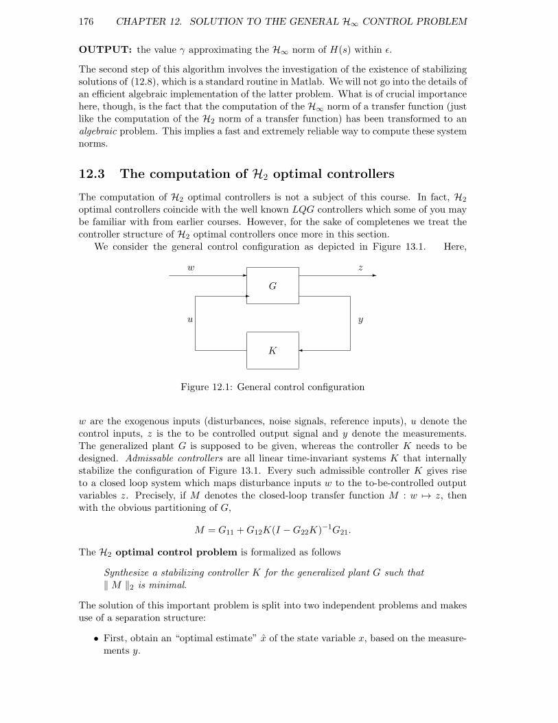
176 CHAPTER 12. SOLUTION TO THE GENERAL H∞ CONTROL PROBLEM
OUTPUT: the value γ approximating the H∞ norm of H(s) within ε.
The second step of this algorithm involves the investigation of the existence of stabilizingsolutions of (12.8), which is a standard routine in Matlab. We will not go into the details ofan efficient algebraic implementation of the latter problem. What is of crucial importancehere, though, is the fact that the computation of the H∞ norm of a transfer function (justlike the computation of the H2 norm of a transfer function) has been transformed to analgebraic problem. This implies a fast and extremely reliable way to compute these systemnorms.
12.3 The computation of H2 optimal controllers
The computation of H2 optimal controllers is not a subject of this course. In fact, H2optimal controllers coincide with the well known LQG controllers which some of you maybe familiar with from earlier courses. However, for the sake of completenes we treat thecontroller structure of H2 optimal controllers once more in this section.
We consider the general control configuration as depicted in Figure 13.1. Here,
G
K
w z
u y
Figure 12.1: General control configuration
w are the exogenous inputs (disturbances, noise signals, reference inputs), u denote thecontrol inputs, z is the to be controlled output signal and y denote the measurements.The generalized plant G is supposed to be given, whereas the controller K needs to bedesigned. Admissable controllers are all linear time-invariant systems K that internallystabilize the configuration of Figure 13.1. Every such admissible controller K gives riseto a closed loop system which maps disturbance inputs w to the to-be-controlled outputvariables z. Precisely, if M denotes the closed-loop transfer function M : w → z, thenwith the obvious partitioning of G,
M = G11 +G12K(I −G22K)−1G21.
The H2 optimal control problem is formalized as follows
Synthesize a stabilizing controller K for the generalized plant G such that‖M ‖2 is minimal.
The solution of this important problem is split into two independent problems and makesuse of a separation structure:
• First, obtain an “optimal estimate” x of the state variable x, based on the measure-ments y.
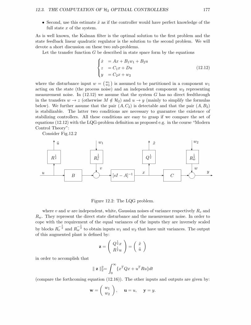
12.3. THE COMPUTATION OF H2 OPTIMAL CONTROLLERS 177
• Second, use this estimate x as if the controller would have perfect knowledge of thefull state x of the system.
As is well known, the Kalman filter is the optimal solution to the first problem and thestate feedback linear quadratic regulator is the solution to the second problem. We willdevote a short discussion on these two sub-problems.
Let the transfer function G be described in state space form by the equationsx = Ax+B1w1 +B2u
z = C1x+Du
y = C2x+ w2
(12.12)
where the disturbance input w =(
w1w2
)is assumed to be partitioned in a component w1
acting on the state (the process noise) and an independent component w2 representingmeasurement noise. In (12.12) we assume that the system G has no direct feedthroughin the transfers w → z (otherwise M /∈ H2) and u → y (mainly to simplify the formulasbelow). We further assume that the pair (A,C2) is detectable and that the pair (A,B2)is stabilizable. The latter two conditions are necessary to guarantee the existence ofstabilizing controllers. All these conditions are easy to grasp if we compare the set ofequations (12.12) with the LQG-problem definition as proposed e.g. in the course “ModernControl Theory”:
Consider Fig.12.2
B [sI −A]−1 C
R12v Q
12 R
12wR
12
u
u
v
w1
x
x
w
w2
y
Figure 12.2: The LQG problem.
where v and w are independent, white, Gaussian noises of variance respectively Rv andRw. They represent the direct state disturbance and the measurement noise. In order tocope with the requirement of the equal variances of the inputs they are inversely scaled
by blocks R− 1
2v and R
− 12
w to obtain inputs w1 and w2 that have unit variances. The outputof this augmented plant is defined by:
z =
(Q
12x
R12u
)=(xu
)in order to accomplish that
‖ z ‖22=∫ ∞
0xTQx+ uTRudt
(compare the forthcoming equation (12.16)). The other inputs and outputs are given by:
w =(w1w2
), u = u, y = y.
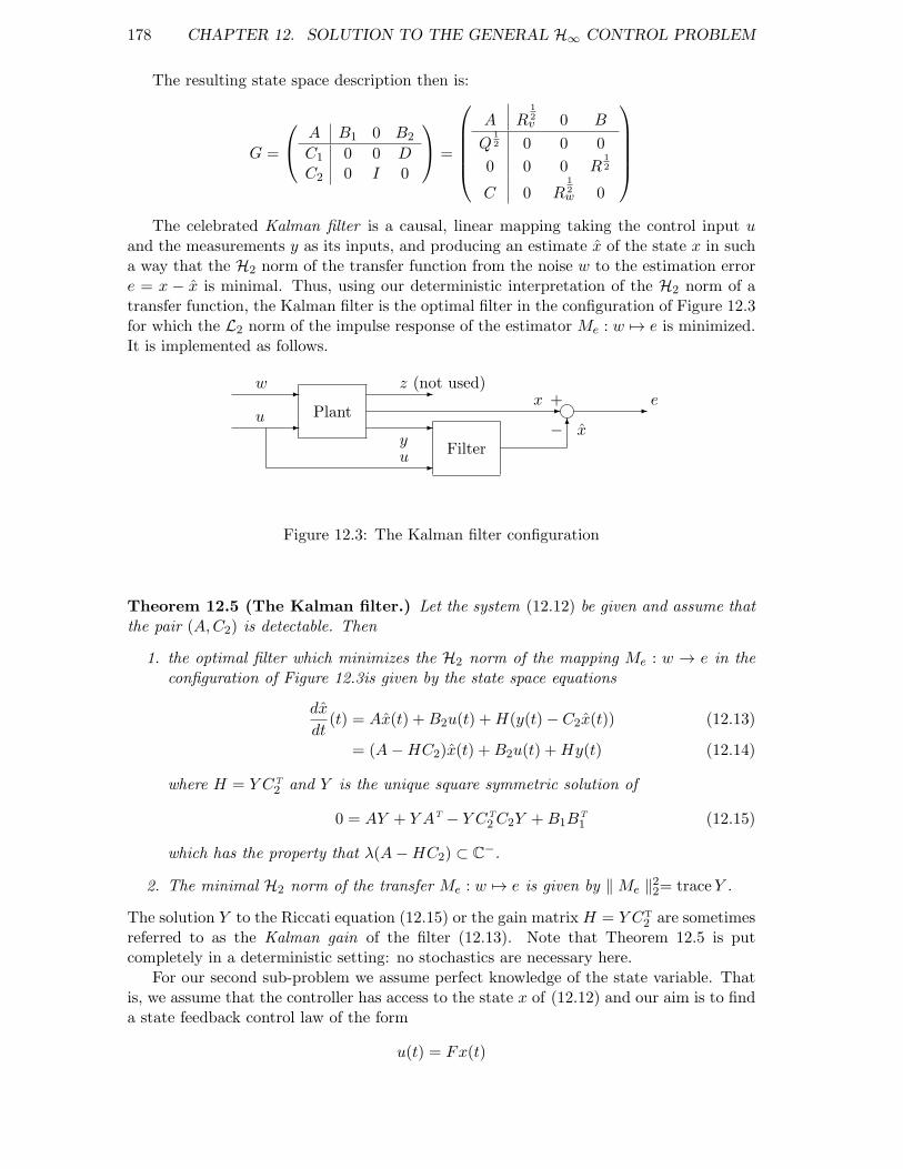
178 CHAPTER 12. SOLUTION TO THE GENERAL H∞ CONTROL PROBLEM
The resulting state space description then is:
G =
A B1 0 B2
C1 0 0 DC2 0 I 0
=
A R
12v 0 B
Q12 0 0 0
0 0 0 R12
C 0 R12w 0
The celebrated Kalman filter is a causal, linear mapping taking the control input u
and the measurements y as its inputs, and producing an estimate x of the state x in sucha way that the H2 norm of the transfer function from the noise w to the estimation errore = x − x is minimal. Thus, using our deterministic interpretation of the H2 norm of atransfer function, the Kalman filter is the optimal filter in the configuration of Figure 12.3for which the L2 norm of the impulse response of the estimator Me : w → e is minimized.It is implemented as follows.
Plant
Filter
w
u
u
y
x +z (not used)
x− e
Figure 12.3: The Kalman filter configuration
Theorem 12.5 (The Kalman filter.) Let the system (12.12) be given and assume thatthe pair (A,C2) is detectable. Then
1. the optimal filter which minimizes the H2 norm of the mapping Me : w → e in theconfiguration of Figure 12.3is given by the state space equations
dx
dt(t) = Ax(t) +B2u(t) +H(y(t)− C2x(t)) (12.13)
= (A−HC2)x(t) +B2u(t) +Hy(t) (12.14)
where H = Y CT2 and Y is the unique square symmetric solution of
0 = AY + Y AT − Y CT2C2Y +B1B
T1 (12.15)
which has the property that λ(A−HC2) ⊂ C−.
2. The minimal H2 norm of the transfer Me : w → e is given by ‖Me ‖22= traceY .
The solution Y to the Riccati equation (12.15) or the gain matrix H = Y CT2 are sometimes
referred to as the Kalman gain of the filter (12.13). Note that Theorem 12.5 is putcompletely in a deterministic setting: no stochastics are necessary here.
For our second sub-problem we assume perfect knowledge of the state variable. Thatis, we assume that the controller has access to the state x of (12.12) and our aim is to finda state feedback control law of the form
u(t) = Fx(t)
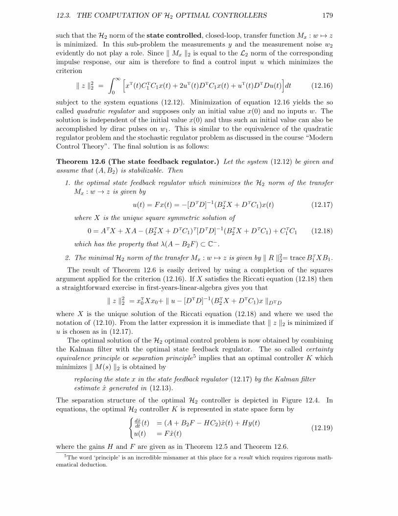
12.3. THE COMPUTATION OF H2 OPTIMAL CONTROLLERS 179
such that the H2 norm of the state controlled, closed-loop, transfer function Mx : w → zis minimized. In this sub-problem the measurements y and the measurement noise w2evidently do not play a role. Since ‖Mx ‖2 is equal to the L2 norm of the correspondingimpulse response, our aim is therefore to find a control input u which minimizes thecriterion
‖ z ‖22 =∫ ∞
0
[xT(t)CT
1C1x(t) + 2uT(t)DTC1x(t) + uT(t)DTDu(t)]dt (12.16)
subject to the system equations (12.12). Minimization of equation 12.16 yields the socalled quadratic regulator and supposes only an initial value x(0) and no inputs w. Thesolution is independent of the initial value x(0) and thus such an initial value can also beaccomplished by dirac pulses on w1. This is similar to the equivalence of the quadraticregulator problem and the stochastic regulator problem as discussed in the course “ModernControl Theory”. The final solution is as follows:
Theorem 12.6 (The state feedback regulator.) Let the system (12.12) be given andassume that (A,B2) is stabilizable. Then
1. the optimal state feedback regulator which minimizes the H2 norm of the transferMx : w → z is given by
u(t) = Fx(t) = −[DTD]−1(BT2X +DTC1)x(t) (12.17)
where X is the unique square symmetric solution of
0 = ATX +XA− (BT2X +DTC1)T[DTD]−1(BT
2X +DTC1) + CT1C1 (12.18)
which has the property that λ(A−B2F ) ⊂ C−.
2. The minimal H2 norm of the transfer Mx : w → z is given by ‖ R ‖22= traceBT1XB1.
The result of Theorem 12.6 is easily derived by using a completion of the squaresargument applied for the criterion (12.16). If X satisfies the Riccati equation (12.18) thena straightforward exercise in first-years-linear-algebra gives you that
‖ z ‖22 = xT0Xx0+ ‖ u− [DTD]−1(BT
2X +DTC1)x ‖DTD
where X is the unique solution of the Riccati equation (12.18) and where we used thenotation of (12.10). From the latter expression it is immediate that ‖ z ‖2 is minimized ifu is chosen as in (12.17).
The optimal solution of the H2 optimal control problem is now obtained by combiningthe Kalman filter with the optimal state feedback regulator. The so called certaintyequivalence principle or separation principle5 implies that an optimal controller K whichminimizes ‖M(s) ‖2 is obtained by
replacing the state x in the state feedback regulator (12.17) by the Kalman filterestimate x generated in (12.13).
The separation structure of the optimal H2 controller is depicted in Figure 12.4. Inequations, the optimal H2 controller K is represented in state space form by
dxdt (t) = (A+B2F −HC2)x(t) +Hy(t)u(t) = Fx(t)
(12.19)
where the gains H and F are given as in Theorem 12.5 and Theorem 12.6.5The word ‘principle’ is an incredible misnamer at this place for a result which requires rigorous math-
ematical deduction.
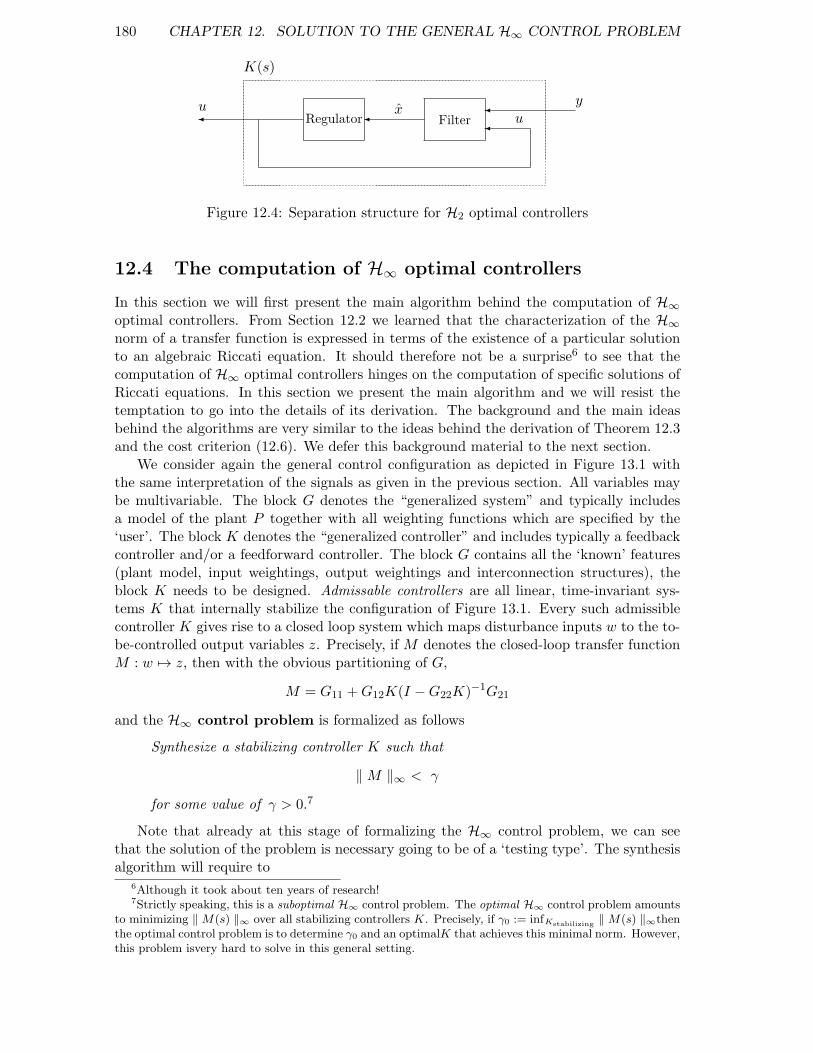
180 CHAPTER 12. SOLUTION TO THE GENERAL H∞ CONTROL PROBLEM
K(s)
Regulator Filter x y
uu
Figure 12.4: Separation structure for H2 optimal controllers
12.4 The computation of H∞ optimal controllers
In this section we will first present the main algorithm behind the computation of H∞optimal controllers. From Section 12.2 we learned that the characterization of the H∞norm of a transfer function is expressed in terms of the existence of a particular solutionto an algebraic Riccati equation. It should therefore not be a surprise6 to see that thecomputation of H∞ optimal controllers hinges on the computation of specific solutions ofRiccati equations. In this section we present the main algorithm and we will resist thetemptation to go into the details of its derivation. The background and the main ideasbehind the algorithms are very similar to the ideas behind the derivation of Theorem 12.3and the cost criterion (12.6). We defer this background material to the next section.
We consider again the general control configuration as depicted in Figure 13.1 withthe same interpretation of the signals as given in the previous section. All variables maybe multivariable. The block G denotes the “generalized system” and typically includesa model of the plant P together with all weighting functions which are specified by the‘user’. The block K denotes the “generalized controller” and includes typically a feedbackcontroller and/or a feedforward controller. The block G contains all the ‘known’ features(plant model, input weightings, output weightings and interconnection structures), theblock K needs to be designed. Admissable controllers are all linear, time-invariant sys-tems K that internally stabilize the configuration of Figure 13.1. Every such admissiblecontroller K gives rise to a closed loop system which maps disturbance inputs w to the to-be-controlled output variables z. Precisely, if M denotes the closed-loop transfer functionM : w → z, then with the obvious partitioning of G,
M = G11 +G12K(I −G22K)−1G21
and the H∞ control problem is formalized as follows
Synthesize a stabilizing controller K such that
‖M ‖∞ < γ
for some value of γ > 0.7
Note that already at this stage of formalizing the H∞ control problem, we can seethat the solution of the problem is necessary going to be of a ‘testing type’. The synthesisalgorithm will require to
6Although it took about ten years of research!7Strictly speaking, this is a suboptimal H∞ control problem. The optimal H∞ control problem amounts
to minimizing ‖ M(s) ‖∞ over all stabilizing controllers K. Precisely, if γ0 := infKstabilizing ‖ M(s) ‖∞thenthe optimal control problem is to determine γ0 and an optimalK that achieves this minimal norm. However,this problem isvery hard to solve in this general setting.
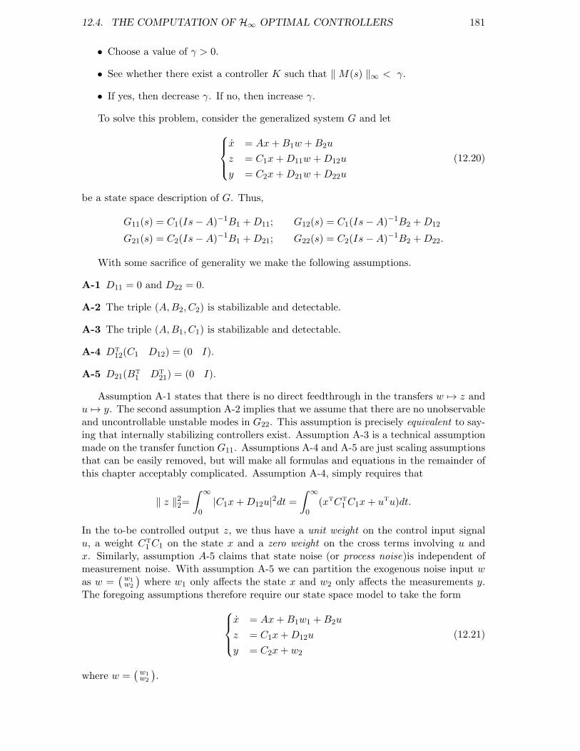
12.4. THE COMPUTATION OF H∞ OPTIMAL CONTROLLERS 181
• Choose a value of γ > 0.
• See whether there exist a controller K such that ‖M(s) ‖∞ < γ.
• If yes, then decrease γ. If no, then increase γ.
To solve this problem, consider the generalized system G and letx = Ax+B1w +B2u
z = C1x+D11w +D12u
y = C2x+D21w +D22u
(12.20)
be a state space description of G. Thus,
G11(s) = C1(Is−A)−1B1 +D11; G12(s) = C1(Is−A)−1B2 +D12
G21(s) = C2(Is−A)−1B1 +D21; G22(s) = C2(Is−A)−1B2 +D22.
With some sacrifice of generality we make the following assumptions.
A-1 D11 = 0 and D22 = 0.
A-2 The triple (A,B2, C2) is stabilizable and detectable.
A-3 The triple (A,B1, C1) is stabilizable and detectable.
A-4 DT12(C1 D12) = (0 I).
A-5 D21(BT1 DT
21) = (0 I).
Assumption A-1 states that there is no direct feedthrough in the transfers w → z andu → y. The second assumption A-2 implies that we assume that there are no unobservableand uncontrollable unstable modes in G22. This assumption is precisely equivalent to say-ing that internally stabilizing controllers exist. Assumption A-3 is a technical assumptionmade on the transfer function G11. Assumptions A-4 and A-5 are just scaling assumptionsthat can be easily removed, but will make all formulas and equations in the remainder ofthis chapter acceptably complicated. Assumption A-4, simply requires that
‖ z ‖22=∫ ∞
0|C1x+D12u|2dt =
∫ ∞
0(xTCT
1C1x+ uTu)dt.
In the to-be controlled output z, we thus have a unit weight on the control input signalu, a weight CT
1C1 on the state x and a zero weight on the cross terms involving u andx. Similarly, assumption A-5 claims that state noise (or process noise)is independent ofmeasurement noise. With assumption A-5 we can partition the exogenous noise input was w =
(w1w2
)where w1 only affects the state x and w2 only affects the measurements y.
The foregoing assumptions therefore require our state space model to take the formx = Ax+B1w1 +B2u
z = C1x+D12u
y = C2x+ w2
(12.21)
where w =(
w1w2
).
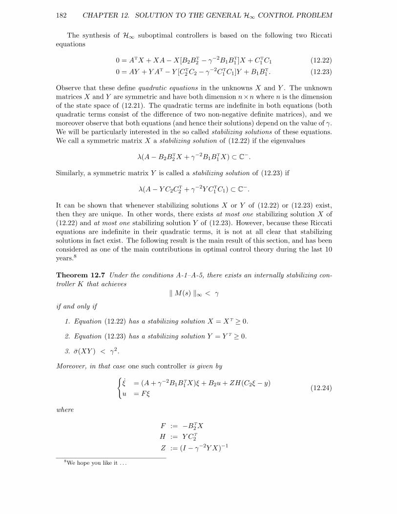
182 CHAPTER 12. SOLUTION TO THE GENERAL H∞ CONTROL PROBLEM
The synthesis of H∞ suboptimal controllers is based on the following two Riccatiequations
0 = ATX +XA−X[B2BT2 − γ−2B1B
T1 ]X + CT
1C1 (12.22)
0 = AY + Y AT − Y [CT2C2 − γ−2CT
1C1]Y +B1BT1 . (12.23)
Observe that these define quadratic equations in the unknowns X and Y . The unknownmatrices X and Y are symmetric and have both dimension n×n where n is the dimensionof the state space of (12.21). The quadratic terms are indefinite in both equations (bothquadratic terms consist of the difference of two non-negative definite matrices), and wemoreover observe that both equations (and hence their solutions) depend on the value of γ.We will be particularly interested in the so called stabilizing solutions of these equations.We call a symmetric matrix X a stabilizing solution of (12.22) if the eigenvalues
λ(A−B2BT2X + γ−2B1B
T1X) ⊂ C−.
Similarly, a symmetric matrix Y is called a stabilizing solution of (12.23) if
λ(A− Y C2CT2 + γ−2Y CT
1C1) ⊂ C−.
It can be shown that whenever stabilizing solutions X or Y of (12.22) or (12.23) exist,then they are unique. In other words, there exists at most one stabilizing solution X of(12.22) and at most one stabilizing solution Y of (12.23). However, because these Riccatiequations are indefinite in their quadratic terms, it is not at all clear that stabilizingsolutions in fact exist. The following result is the main result of this section, and has beenconsidered as one of the main contributions in optimal control theory during the last 10years.8
Theorem 12.7 Under the conditions A-1–A-5, there exists an internally stabilizing con-troller K that achieves
‖M(s) ‖∞ < γ
if and only if
1. Equation (12.22) has a stabilizing solution X = XT ≥ 0.
2. Equation (12.23) has a stabilizing solution Y = Y T ≥ 0.
3. σ(XY ) < γ2.
Moreover, in that case one such controller is given byξ = (A+ γ−2B1B
T1X)ξ +B2u+ ZH(C2ξ − y)
u = Fξ(12.24)
where
F := −BT2X
H := Y CT2
Z := (I − γ−2Y X)−1
8We hope you like it . . .
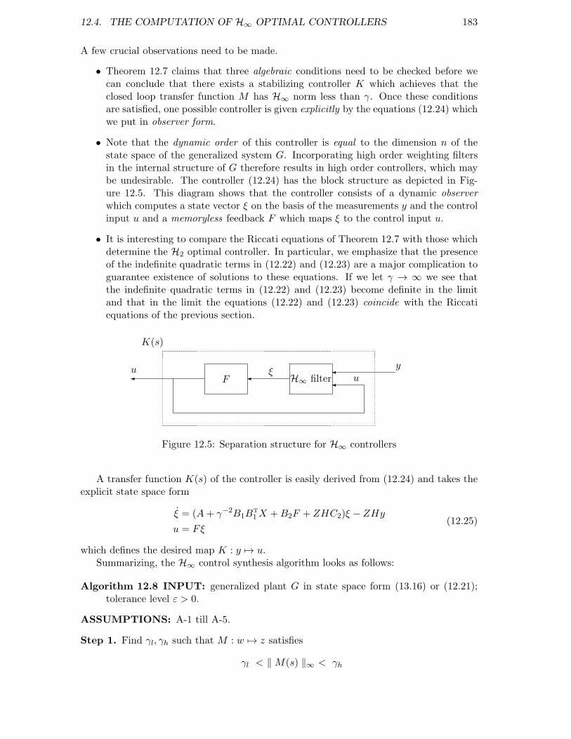
12.4. THE COMPUTATION OF H∞ OPTIMAL CONTROLLERS 183
A few crucial observations need to be made.
• Theorem 12.7 claims that three algebraic conditions need to be checked before wecan conclude that there exists a stabilizing controller K which achieves that theclosed loop transfer function M has H∞ norm less than γ. Once these conditionsare satisfied, one possible controller is given explicitly by the equations (12.24) whichwe put in observer form.
• Note that the dynamic order of this controller is equal to the dimension n of thestate space of the generalized system G. Incorporating high order weighting filtersin the internal structure of G therefore results in high order controllers, which maybe undesirable. The controller (12.24) has the block structure as depicted in Fig-ure 12.5. This diagram shows that the controller consists of a dynamic observerwhich computes a state vector ξ on the basis of the measurements y and the controlinput u and a memoryless feedback F which maps ξ to the control input u.
• It is interesting to compare the Riccati equations of Theorem 12.7 with those whichdetermine the H2 optimal controller. In particular, we emphasize that the presenceof the indefinite quadratic terms in (12.22) and (12.23) are a major complication toguarantee existence of solutions to these equations. If we let γ → ∞ we see thatthe indefinite quadratic terms in (12.22) and (12.23) become definite in the limitand that in the limit the equations (12.22) and (12.23) coincide with the Riccatiequations of the previous section.
K(s)
F H∞ filter ξ y
uu
Figure 12.5: Separation structure for H∞ controllers
A transfer function K(s) of the controller is easily derived from (12.24) and takes theexplicit state space form
ξ = (A+ γ−2B1BT1X +B2F + ZHC2)ξ − ZHy
u = Fξ(12.25)
which defines the desired map K : y → u.Summarizing, the H∞ control synthesis algorithm looks as follows:
Algorithm 12.8 INPUT: generalized plant G in state space form (13.16) or (12.21);tolerance level ε > 0.
ASSUMPTIONS: A-1 till A-5.
Step 1. Find γl, γh such that M : w → z satisfies
γl < ‖M(s) ‖∞ < γh
184 CHAPTER 12. SOLUTION TO THE GENERAL H∞ CONTROL PROBLEM
Step 2. Let γ := (γl + γh)/2 and verify whether there exists matrices X = XT andY = Y T satisfying the conditions 1–3 of Theorem 12.7.
Step 3. If so, then set γh = γ. If not, then set γl = γ.
Step 4. Put ε = γh − γl.
Step 5. If ε > ε then go to Step 2.
Step 6. Put γ = γh and letξ = (A+ γ−2B1B
T1X +B2F + ZHC2)ξ − ZHy
u = Fξ
define the state space equations of a controller K(s).
OUTPUT: K(s) defines a stabilizing controller which achieves ‖M(s) ‖∞ < γ.
12.5 The state feedback H∞ control problem
The results of the previous section can not fully be appreciated if no further systemtheoretic insight is given in the main results. In this section we will treat the statefeedback H∞ optimal control problem, which is a special case of Theorem 12.7 and whichprovides quite some insight in the structure of optimal H∞ control laws.
In this section we will therefore assume that the controller K(s) has access to the fullstate x, i.e., we assume that the measurements y = x and we wish to design a controllerK(s) for which the closed loop transfer function, alternatively indicated here by Mx :w → z satisfies‖ Mx ‖∞ < γ. The procedure to obtain such a controller is basically aninteresting extension of thearguments we put forward in section 12.2.
The criterion (12.6) defined in section 12.2 only depends on the initial condition x0of the state and the input w of the system (12.1). Since we are now dealing with thesystem (12.21) with state measurements (y = x) and two inputs u and w, we should treatthe criterion
J(x0, u, w) := ‖ z ‖22 −γ2 ‖ w ‖2=∫ ∞
0
(|z(t)|2 − γ2|w(t)|2
)dt,
(12.26)
as a function of the initial state x0 and both the control inputs u as well as the disturbanceinputs w. Here z is of course the output of the system (12.21) when the inputs u and ware applied and the initial state x(0) is taken to be x0.
We will view the criterion (12.26) as a game between two players. One player, u, aimsto minimize the criterion J , while the other player, w, aims to maximize it.9 We call apair of strategies (u∗, w∗) optimal with respect to the criterion J(x0, u, w) if for all u ∈ L2and w ∈ L2 the inequalities
J(x0, u∗, w) ≤ J(x0, u
∗, w∗) ≤ J(x0, u, w∗) (12.27)
9Just like a soccer match where instead of administrating the number of goals of each team, thedifference between the number of goals is taken as the relevant performance criterion. After all, this is theonly relevant criterion which counts at the end of a soccer game . . . .
12.6. THE H∞ FILTERING PROBLEM 185
are satisfied. Such a pair (u∗, w∗) defines a saddle point for the criterion J . We may thinkof u∗ as a best control strategy, while w∗ is the worst exogenous input. The existenceof such a saddle point is guaranteed by the solutions X of the Riccati equation (12.22).Specifically, under the assumptions made in the previous section, for any solution Xof (12.22) a completion of the squares argument will give you that for all pairs (u,w) of(square integrable) inputs of the system (12.21) for which limt→∞ x(t) = 0 there holds
J(x0, u, w) = xT0Xx0+ ‖ w − γ−2BT
1Xx ‖22 − ‖ u+BT2Xx ‖22 . (12.28)
Thus, if both ‘players’ u and w have access to the state x of (12.21) then (12.28) gives usimmediately a saddle point
u∗(t) := −BT2Xx(t)
w∗(t) := γ−2B1Xx(t)
which satisfies the inequalities (12.27). We see that in that case the saddle point
J(x0, u∗, w∗) = xT
0Xx0
which gives a nice interpretation of the solution X of the Riccati equation (12.22). Now,taking the initial state x0 = 0 gives that the saddle point J(0, u∗, w∗) = 0 which, by (12.27)gives that for all w ∈ L2
J(0, u∗, w) ≤ J(0, u∗, w∗) = 0
As in section 12.2 it thus follows that the closed loop system Mx : w → z obtained byapplying the static state feedback controller
u∗(t) = −BT2Xx(t)
results in ‖ Mx(s) ‖∞ ≤ γ. We moreover see from this analysis that the worst casedisturbance is generated by w∗.
12.6 The H∞ filtering problem
Just like we splitted the optimal H2 control problem into a state feedback problem and afiltering problem, the H∞ control problem admits a similar separation. The H∞ filteringproblem is the subject of this section and can be formalized as follows.
We reconsider the state space equations (12.21):x = Ax+B1w1 +B2u
z = C1x+D12u
y = C2x+ w2
(12.29)
under the same conditions as in the previous section.Just like the Kalman filter, the H∞ filter is a causal, linear mapping taking the control
input u and the measurements y as its inputs, and producing an estimate z of the signal zin such a way that theH∞ norm of the transfer function from the noise w to the estimationerror e = z − z is minimal. Thus, in the configuration of Figure 12.6, we wish to designa filter mapping (u, y) → z such that the for overall configuration with transfer functionMe : w → e the H∞ norm
‖Me(s) ‖2∞ = supw1,w2∈L2
‖ e ‖22‖ w1 ‖22 + ‖ w2 ‖22
(12.30)
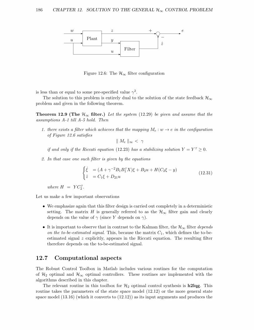
186 CHAPTER 12. SOLUTION TO THE GENERAL H∞ CONTROL PROBLEM
Plant
Filter
w
u
u
y
z +
z
− e
Figure 12.6: The H∞ filter configuration
is less than or equal to some pre-specified value γ2.The solution to this problem is entirely dual to the solution of the state feedback H∞
problem and given in the following theorem.
Theorem 12.9 (The H∞ filter.) Let the system (12.29) be given and assume that theassumptions A-1 till A-5 hold. Then
1. there exists a filter which achieves that the mapping Me : w → e in the configurationof Figure 12.6 satisfies
‖Me ‖∞ < γ
if and only if the Riccati equation (12.23) has a stabilizing solution Y = Y T ≥ 0.
2. In that case one such filter is given by the equationsξ = (A+ γ−2B1B
T1X)ξ +B2u+H(C2ξ − y)
z = C1ξ +D21u(12.31)
where H = Y CT2 .
Let us make a few important observations
• We emphasize again that this filter design is carried out completely in a deterministicsetting. The matrix H is generally referred to as the H∞ filter gain and clearlydepends on the value of γ (since Y depends on γ).
• It is important to observe that in contrast to the Kalman filter, theH∞ filter dependson the to-be-estimated signal. This, because the matrix C1, which defines the to-be-estimated signal z explicitly, appears in the Riccati equation. The resulting filtertherefore depends on the to-be-estimated signal.
12.7 Computational aspects
The Robust Control Toolbox in Matlab includes various routines for the computationof H2 optimal and H∞ optimal controllers. These routines are implemented with thealgorithms described in this chapter.
The relevant routine in this toolbox for H2 optimal control synthesis is h2lqg. Thisroutine takes the parameters of the state space model (12.12) or the more general statespace model (13.16) (which it converts to (12.12)) as its input arguments and produces the

12.8. EXERCISES 187
state space matrices (Ac,Bc,Cc,Dc) of the optimal H2 controller as defined in (12.19)as its outputs. If desired, this routine also produces the state space description of thecorresponding closed-loop transfer function M as its output. (See the corresponding helpfile).
ForH∞ optimal control synthesis, the Robust Control Toolbox includes an efficient im-plementation of the result mentioned in Theorem 12.7. The Matlab routine hinf takes thestate space parameters of the model (13.16) as its input arguments and produces the statespace parameters of the so called central controller as specified by the formulae (12.24) inTheorem 12.7. The routine makes use of the two Riccati solution as presented above. Alsothe state space parameters of the corresponding closed loop system can be obtained asan optional output argument. The Robust Control Toolbox provides features to quicklygenerate augmented plants which incorporate suitable weighting filters. An efficient use ofthese routines, however, requires quite some programming effort in Matlab. Although weconsider this an excellent exercise it is not really the purpose of this course. The packageMHC (Multivariable H∞ Control Design) has been written as part of a PhD study byone of the students of the Measurement and Control Group at TUE, and has been cus-tomized to easily experiment with filter design. During this course we will give a softwaredemonstration of this package.
12.8 Exercises
Exercise 0. Take the first blockscheme of the exercise of chapter 6. Define a mixedsensitivity problem where the performance is represented by good tracking. FilterWe is low pass and has to be chosen. The robustness term is defined by a boundedadditive model error: ‖Wx
−1∆P ‖∞< 1.
Furthermore,‖ r ‖2< 1, P = (s− 1)/(s+ 1) and Wx = s/(s+ 3). What bandwidthcan you obtain for the sensitivity being less than .01 ? Use the tool MHC!
Exercise 1. Write a routine h2comp in MATLAB which computes the H2 norm of atransfer function H(s). Let the state space parameters (A,B,C,D) be the input tothis routine, and the H2 norm
‖ C(Is−A)−1B +D ‖2its output. Build in sufficient checks on the matrices (A,B,C,D) to guarantee a‘fool-proof’ behavior of the routine.
Hint: Use the Theorem 12.1. See the help files of the routines lyap in the control systemtoolbox to solve the Lyapunov equation (12.2). The procedures abcdchk, minreal, eig, orobsv may prove helpful.
Exercise 2. Write a block diagram for the optimal H2 controller and for the optimal H∞controller.
Exercise 3. Suppose that a stable transfer function H(s) admits the state space repre-sentation
x = Ax+Bw
z = Cx+Dw.
Show that ‖ H(s) ‖∞ < γ implies that γ2I − DTD is positive definite. Give anexample of a system for which the converse is not true, i.e., give an example forwhich γ2I −DTD is positive definite and ‖ H(s) ‖∞ > γ.
188 CHAPTER 12. SOLUTION TO THE GENERAL H∞ CONTROL PROBLEM
Exercise 4. This exercise is a more extensive simulation exercise. Using MATLAB andthe installed package MHC (Multivariable H∞ Controller design) you should be ableto design a robust controller for the following problem. You may also like to use theMHC package that has been demonstrated and for which a manual is available uponrequest.
The system considered in this design is a satellite with two highly flexible solar arraysattached. The model for control analysis represents the transfer function from thetorque applied to the roll axis of the satellite to the corresponding satellite roll angle.In order to keep the model simple, only a rigid body mode and a single flexible modeare included, resulting in a four state model. The state space system is described by
x = Ax+Bu+Bw
y = Cx
where u is the control torque (in units Nm), w is a constant disturbance torque(Nm), and y is the roll angle measurement (in rad). The state space matrices aregiven by
A =
0 1 0 00 0 0 00 0 0 10 0 −ω2 −2ζω
; B =
0
1.7319× 10⁻⁵
03.7859× 10⁻⁴
;
C =(1 0 1 0
); D = 0.
where ω = 1.539rad/sec is the frequency of the flexible mode and ζ = 0.003 is theflexural damping ratio. The nominal open loop poles are at
−0.0046 + 1.5390j, −0.0046− 1.5390j, 0
and the finite zeros at
−0.0002 + 0.3219j, −0.0002− 0.3219j.
Because of the highly flexible nature of this system, the use of control torque forattitude control can lead to excitation of the lightly damped flexural modes andhence loss of control. It is therefore desired to design a feedback controller whichincreases the system damping and maintains a specified pointing accuracy. Thatis, variations in the roll angle are to be limited in the face of torque disturbances.In addition the stiffness of the structure is uncertain, and the natural frequency, ω,can only be approximately estimated. Hence, it is desirable that the closed loop berobustly stable to variations in this parameter.
The design objectives are as follows.
1. Performance: required pointing accuracy due to 0.3Nm step torque distur-bance should be y(t) < 0.0007 rad for all t > 0. Additionally, the responsetime is required to be less than 1 minute (60sec).
2. Robust stability: stable response for about 10% variations in the naturalfrequency ω.
3. Control level: control effort due to 0.3Nm step torque disturbances u(t) <0.5 Nm.
12.8. EXERCISES 189
We will start the design by making a few simple observations
• Verify that with a feedback control law u = −Cy the resulting closed-looptransfer U := (I + PC)−1P maps the torque disturbance w to the roll angle y.
• Note that, to achieve a pointing accuracy of 0.0007rad in the face of 0.3Nmtorque input disturbances, we require that U satisfies the condition
σ(U) = σ(I + PC)−1P <0.0007
0.3= 0.0021 rad/Nm (12.32)
at least at low frequencies.
• Recall that, for a suitable weighting function W we can achieve that |U(jω)| ≤γ
|W (jω)| for all ω, where γ is the usual parameter in the ‘γ–iteration’ of the H∞optimization procedure.
Consider the weighting filter
Wk(s) = ks+ 0.4s+ 0.001
(12.33)
where k is a positive constant.
1. Determine a value of k so as to achieve the required level of pointing accuracyin the H∞ design. Try to obtain a value of γ which is more or less equal to 1.Hint: Set up a scheme for H∞ controller design in which the output y+10−5w is usedas a measurement variable and in which the to be controlled variables are
z =(
Wky10−5u
)(the extra output is necessary to regularize the design). Use the MHC package tocompute a suboptimal H∞ controller C which minimizes the H∞ norm of the closedloop transfer w → z for various values of k > 0. Construct a 0.3Nm step torqueinput disturbance w to verify whether your closed-loop system meets the pointingspecification. See the MHC help facility to get more details.
2. Let Wk be given by the filter (12.33) with k as determined in 2. Let V (s) bea second weighting filter and consider the weighted control sensitivity M :=WkUV = Wk(I +PC)−1PV . Choose V in such a way that an H∞ suboptimalcontroller C which minimizes ‖M ‖∞ meets the design specifications.Hint: Use the same configuration as in part 2 and compute controllers C by using thepackage MHC and by varying the weighting filter V .
3. After you complete the design phase, make Bode plots of the closed-loop re-sponse of the system and verify whether the specifications are met by perturbingthe parameter ω and by plotting the closed–loop system responses of the signalsu and y under step torque disturbances of 0.3Nm.

190 CHAPTER 12. SOLUTION TO THE GENERAL H∞ CONTROL PROBLEM
Chapter 13
Solution to the general H∞ controlproblem
In previous chapters we have been mainly concerned with properties of control config-urations in which a controller is designed so as to minimize the H∞ norm of a closedloop transfer function. So far, we did not address the question how such a controller isactually computed. This has been a problem of main concern in the early 80-s. Variousmathematical techniques have been developed to compute H∞-optimal controllers, i.e.,feedback controllers which stabilize a closed loop system and at the same time minimizethe H∞ norm of a closed loop transfer function. In this chapter we treat a solution to amost general version of the H∞ optimal control problem. We will make use of a techniquewhich is based on Linear Matrix Inequalities (LMI’s). This technique is fast, simple, andat the same time a most reliable and efficient way to synthesize H∞ optimal controllers.This chapter is organized as follows. In the next section we first treat the concept ofa dissipative dynamical system. We will see that linear dissipative systems are closepyrelated to Linear Matrix Inequalities (LMI’s) and we will subsequently show how the H∞norm of a transfer function can be computed by means of LMI’s. Finally, we consider thesynthesis question of how to obtain a controller which stabilizes a given dynamical systemso as to minimize the H∞ norm of the closed loop system. Proofs of theorems are includedfor completeness only. They are not part of the material of the course and can be skippedupon first reading of the chapter.
13.1 Dissipative dynamical systems
13.1.1 Introduction
The notion of dissipativity (or passivity) is motivated by the idea of energy dissipation inmany physical dynamical systems. It is a most important concept in system theory anddissipativity plays a crucial role in many modeling questions. Especially in the physicalsciences, dissipativity is closely related to the notion of energy. Roughly speaking, adissipative system is characterized by the property that at any time the amount of energywhich the system can conceivably supply to its environment can not exceed the amountof energy that has been supplied to it. Stated otherwise, when time evolves a dissipativesystem absorbs a fraction of its supplied energy and transforms it for example into heat,an increase of entropy, mass, electromagnetic radiation, or other kinds of energy ‘losses’.In many applications, the question whether a system is dissipative or not can be answeredfrom physical considerations on the way the system interacts with its environment. For
191
192 CHAPTER 13. SOLUTION TO THE GENERAL H∞ CONTROL PROBLEM
example, by observing that the system is an interconnection of dissipative components, orby considering systems in which a loss of energy is inherent to the behavior of the system(due to friction, optical dispersion, evaporation losses, etc.).
In this chapter we will formalize the notion of a dissipative dynamical system for theclass of linear time-invariant systems. It will be shown that linear matrix inequalities(LMI’s) occur in a very natural way in the study of linear dissipative systems. Solutionsof these inequalities have a natural interpretation as storage functions associated with adissipative dyamical system. This interpretation will play a key role in understandingthe relation between LMI’s and questions related to stability, robustness, and H∞ con-troller design. In recent years, linear matrix inequalities have emerged as a powerful toolto approach control problems that appear hard if not impossible to solve in an analyticfashion. Although the history of LMI’s goes back to the fourties with a major emphasis oftheir role in control in the sixties (Kalman, Yakubovich, Popov, Willems), only recentlypowerful numerical interior point techniques have been developed to solve LMI’s in a prac-tically efficient manner (Nesterov, Nemirovskii 1994). Several Matlab software packagesare available that allow a simple coding of general LMI problems and of those that arisein typical control problems (LMI Control Toolbox, LMI-tool).
13.1.2 Dissipativity
Consider a continuous time, time-invariant dynamical system Σ described by the equa-tions1
Σ :
x = Ax+Bu
y = Cx+Du(13.1)
As usual, x is the state which takes its values in a state space X = Rn, u is the inputtaking its values in an input space U = Rm and y denotes the output of the system whichassumes its values in the output space Y = Rp. Let
s : U × Y → R
be a mapping and assume that for all time instances t0, t1 ∈ R and for all input-outputpairs u, y satisfying (13.1) the function
s(t) := s(u(t), y(t))
is locally integrable, i.e.,∫ t1t0|s(t)|dt <∞. The mapping s will be referred to as the supply
function.
Definition 13.1 (Dissipativity) The system Σ with supply rate s is said to be dissipa-tive if there exists a non-negative function V : X → R such that
V (x(t0)) +∫ t1
t0
s(t)dt ≥ V (x(t1)) (13.2)
for all t0 ≤ t1 and all trajectories (u, x, y) which satisfy (13.1).
1Much of what is said in this chapter can be applied for (much) more general systems of the formx = f(x, u), y = g(x, u).
13.1. DISSIPATIVE DYNAMICAL SYSTEMS 193
Interpretation 13.2 The supply function (or supply rate) s should be interpreted as thesupply delivered to the system. This means that in a time interval [0, t] work has beendone on the system whenever
∫ t0 s(τ)dτ is positive, while work is done by the system
if this integral is negative. The non-negative function V is called a storage functionand generalizes the notion of an energy function for a dissipative system. With thisinterpretation, inequality (13.2) formalizes the intuitive idea that a dissipative system ischaracterized by the property that the change of internal storage (V (x(t1)) − V (x(t0)))in any time interval [t0, t1] will never exceed the amount of supply that flows into thesystem (or the ‘work done on the system). This means that part of what is supplied tothe system is stored, while the remaining part is dissipated. Inequality (13.2) is known asthe dissipation inequality.
Remark 13.3 If the function V (x(·)) with V a storage function and x : R → X a statetrajectory of (13.1) is differentiable as a function of time, then (13.2) can be equivalentlywritten as
V (t) ≤ s(u(t), y(t)). (13.3)
Remark 13.4 (this remark may be skipped) There is a refinement of Definition 13.1which is worth mentioning. The system Σ is said to be conservative (or lossless) if thereexists a non-negative function V : X → R such that equality holds in (13.2) for all t0 ≤ t1and all (u, x, y) which satisfy (13.1). .
Example 13.5 Consider an electrical network with n external ports. Denote the externalvoltages and currents of the i-th port by (Vi, Ii) and let V and I denote the vectors of lengthn whose i-th component is Vi and Ii, respectively. Assume that the network contains (afinite number of) resistors, capacitors, inductors and lossless elements such as transformersand gyrators. Let nC and nL denote the number of capacitors and inductors in the networkand denote by VC and IL the vectors of voltage drops accrioss the capacitors and currentsthrough the inductors of the network. An impedance description of the system then takesthe form (13.1), where u = I, y = V and x =
(V T
C ITL
)T. For such a circuit, a naturalsupply function is
s(V (t), I(t)) = V T(t)I(t).
This system is dissipative and
V (x) :=nC∑i=1
CiV2Ci
+nL∑i=1
LiI2Li
is a storage function of the system that represents the total electrical energy in the capac-itors and inductors.
Example 13.6 Consider a thermodynamic system at uniform temperature T on whichmechanical work is being done at rate W and which is being heated at rate Q. Let(T,Q,W ) be the external variables of such a system and assume that –either by physicalor chemical principles or through experimentation– the mathematical model of the ther-modynamic system has been decided upon and is given by the time invariant system (13.1).The first and second law of thermodynamics may then be formulated in the sense of Defi-nition 13.1 by saying that the system Σ is conservative with respect to the supply functions1 := (W +Q) and dissipative with respect to the supply function s2 := −Q/T . Indeed,
194 CHAPTER 13. SOLUTION TO THE GENERAL H∞ CONTROL PROBLEM
the two basic laws of thermodynamics state that for all system trajectories (T,Q,W ) andall time instants t0 ≤ t1
E(x(t0)) +∫ t1
t0
Q(t) +W (t) dt = E(x(t1))
(which is conservation of thermodynamical energy) and the second law of thermodynamicsstates that the system trajectories satisfy
S(x(t0)) +∫ t1
t0
−Q(t)T (t)
dt ≥ S(x(t1))
for a storage function S. Here, E is called the internal energy and S the entropy. Thefirst law promises that the change of internal energy is equal to the heat absorbed by thesystem and the mechanical work which is done on the system. The second law states thatthe entropy decreases at a higher rate than the quotient of absorbed heat and temperature.Note that thermodynamical systems are dissipative with respect to more than one supplyfunction!
Example 13.7 As another example, the product of forces and velocities is a candidatesupply function in mechanical systems. For those familiar with the theory of bond-graphswe remark that every bond-graph can be viewed as a representation of a dissipative dy-namical system where input and output variables are taken to be effort and flow variablesand the supply function s is invariably taken to be the product of these two variables.A bond-graph is therefore a special case of a dissipative system (and not the other wayaround!).
Example 13.8 Typical examples of supply functions s : U × Y → R are
s(u, y) = uTy, (13.4)
s(u, y) = ‖y‖2 − ‖u‖2 (13.5)
s(u, y) = ‖y‖2 + ‖u‖2 (13.6)
s(u, y) = ‖y‖2 (13.7)
which arise in network theory, bondgraph theory, scattering theory, H∞ theory, gametheory, LQ-optimal control and H2-optimal control theory.
If Σ is dissipative with storage function V , then we will assume that there exists areference point x∗ ∈ X of minimal storage, i.e. there exists x∗ ∈ X such that V (x∗) =minx∈X V (x). You can think of x∗ as the state in which the system is ‘at rest’, an‘equilibrium state’ for which no energy is stored in the system. Given a storage functionV , its normalization (with respect to x∗) is defined as V (x) := V (x)− V (x∗). Obviously,V (x∗) = 0 and V is a storage function of Σ whenever V is. For linear systems of the form(13.1) we usually take x∗ = 0.
13.1.3 A first characterization of dissipativity
Instead of considering the set of all possible storage functions associated with a dynamicalsystem Σ, we will restrict attention to the set of normalized storage functions. Formally,the set of normalized storage functions (associated with (Σ, s)) is defined by
V(x∗) := V : X → R+ | V (x∗) = 0 and (13.2) holds.
13.1. DISSIPATIVE DYNAMICAL SYSTEMS 195
The existence of a reference point x∗ of minimal storage implies that for a dissipativesystem ∫ t1
0s(u(t), y(t)) dt ≥ 0
for any t1 ≥ 0 and any (u, x, y) satisfying (13.1) with x(0) = x∗. Stated otherwise, anytrajectory of the system which emanates from x∗ has the property that the net flow ofsupply is into the system. In many treatments of dissipativity this property is often takenas definition of passivity.
We introduce two mappings Vav : X → R+ ∪∞ and Vreq : X → R ∪ −∞ which willplay a crucial role in the sequel. They are defined by
Vav(x0) := sup−∫ t1
0s(t) dt | t1 ≥ 0; (u, x, y) satisfy (13.1) with x(0) = x0
(13.8a)
Vreq(x0) := inf
∫ 0
t−1
s(t) dt | t−1 ≤ 0; (u, x, y) satisfy (13.1) with (13.8b)
x(0) = x0 and x(t−1) = x∗
Interpretation 13.9 Vav(x) denotes the maximal amount of internal storage that maybe recovered from the system over all state trajectories starting from x. Similarly, Vreq(x)reflects the minimal supply the environment has to deliver to the system in order to excitethe state x via any trajectory in the state space originating in x∗.
We refer to Vav and Vreq as the available storage and the required supply, respectively. Notethat in (13.8b) it is assumed that the point x0 ∈ X is reachable from the reference pontx∗, i.e. it is assumed that there exist a control input u which brings the state trajectoryx from x∗ at time t = t−1 to x0 at time t = 0. This is possible when the system Σ iscontrollable.
Theorem 13.10 Let the system Σ be described by (13.1) and let s be a supply function.Then
1. Σ is dissipative if and only if Vav(x) is finite for all x ∈ X.
2. If Σ is dissipative and controllable then
(a) Vav, Vreq ∈ V(x∗).(b) V ∈ V(x∗) ⇒ For all x ∈ X there holds 0 ≤ Vav(x) ≤ V (x) ≤ Vreq(x).
Interpretation 13.11 Theorem 13.10 gives a necessary and sufficient condition for asystem to be dissipative. It shows that both the available storage and the required supplyare possible storage functions. Moreover, statement (b) shows that the available storageand the required supply are the extremal storage functions in V(x∗). In particular, for anystate of a dissipative system, the available storage is at most equal to the required supply.
Proof. 1. Let Σ be dissipative, V a storage function and x0 ∈ X. From (13.2) it then followsthat for all t1 ≥ 0 and all (u, x, y) satisfing (13.1) with x(0) = x0,
−∫ t1
0s(u(t), y(t))dt ≤ V (x0) <∞.
Taking the supremum over all t1 ≥ 0 and all such trajectories (u, x, y) (with x(0) = x0) yields thatVav(x0) ≤ V (x0) < ∞. To prove the converse implication it suffices to show that Vav is a storage
196 CHAPTER 13. SOLUTION TO THE GENERAL H∞ CONTROL PROBLEM
function. To see this, first note that Vav(x) ≥ 0 for all x ∈ X (take t1 = 0 in (13.8a)). To provethat Vav satisfies (13.2), let t0 ≤ t1 ≤ t2 and (u, x, y) satisfy (13.1). Then
Vav(x(t0)) ≥ −∫ t1
t0
s(u(t), y(t))dt−∫ t2
t1
s(u(t), y(t))dt.
Since the second term in the right hand side of this inequality holds for arbitrary t2 ≥ t1 andarbitrary (u, x, y)|[t1,t2] (with x(t1) fixed), we can take the supremum over all such trajectories toconclude that
Vav(x(t0)) ≥ −∫ t1
t0
s(u(t), y(t))dt− Vav(x(t1)).
which shows that Vav satisfies (13.2).2a. Suppose that Σ is dissipative and let V be a storage function. Then V (x) := V (x)−V (x∗) ∈
V(x∗) so that V(x∗) = ∅. Observe that Vav(x∗) ≥ 0 and Vreq(x∗) ≤ 0 (take t1 = t−1 = 0 in(13.8)). Suppose that the latter inequalities are strict. Then, using controllability of the system,there exists t−1 ≤ 0 ≤ t1 and a state trajectory x with x(t−1) = x(0) = x(t1) = x∗ suchthat − ∫ t1
0 s(t)dt > 0 and∫ 0
t−1s(t)dt < 0. But this yields a contradiction with (13.2) as both∫ t1
0 s(t)dt ≥ 0 and∫ 0
t−1s(t)dt ≥ 0. Thus, Vav(x∗) = Vreq(x∗) = 0. We already proved that Vav is a
storage function so that Vav ∈ V(x∗). Along the same lines one shows that also Vreq ∈ V(x∗).2b. If V ∈ V(x∗) then
−∫ t1
0s(u(t), y(t))dt ≤ V (x0) ≤
∫ 0
t−1
s(u(t), y(t))dt
for all t−1 ≤ 0 ≤ t1 and (u, x, y) satisfying (13.1) with x(t−1) = x∗ and x(0) = x0. Now take thesupremum and infimum over all such trajectories to obtain that Vav ≤ V ≤ Vreq.
13.2 Dissipative systems with quadratic supply functions
13.2.1 Quadratic supply functions
In this section we will apply the above theory by considering systems of the form (13.1)with quadratic supply functions s : U × Y → R, defined by
s(u, y) =(yu
)T(Qyy Qyu
Quy Quu
)(yu
)(13.9)
Here,
Q :=(Qyy Qyu
Quy Quu
)is a real symmetric matrix (i.e. Q = QT) which is partitioned conformally with u andy. Note that the supply functions given in Example 13.8 can all be written in the form(13.9).
Remark 13.12 Substituting the output equation y = Cx + Du in the supply function(13.9) shows that (13.9) can equivalently be viewed as a quadratic function in the variablesu and x. Indeed,
s(u, y) = s(u,Cx+Du) =(xu
)T(Qxx Qxu
Qux Quu
)(xu
)where (
Qxx Qxu
Qux Quu
)=(C D0 I
)T(Qyy Qyu
Quy Quu
)(C D0 I
).

13.2. DISSIPATIVE SYSTEMS WITH QUADRATIC SUPPLY FUNCTIONS 197
13.2.2 Complete characterizations of dissipativity
The following theorem is the main result of this section. It provides necessary and sufficientconditions for dissipativeness.
Theorem 13.13 Suppose that the system Σ described by (13.1) is controllable and letG(s) = C(Is−A)−1B+D be the corresponding transfer function. Let the supply functions be defined by (13.9). Then the following statements are equivalent.
1. (Σ, s) is dissipative.
2. (Σ, s) admits a quadratic storage function V (x) := xTKx with K = KT ≥ 0.
3. There exists K = KT ≥ 0 such that
F (K) := −(ATK +KA KB
BTK 0
)+(C D0 I
)T(Qyy Qyu
Quy Quu
)(C D0 I
)≥ 0. (13.10)
4. There exists K− = KT− ≥ 0 such that Vav(x) = xTK−x.
5. There exists K+ = KT+ ≥ 0 such that Vreq(x) = xTK+x.
6. For all ω ∈ R with det(jωI −A) = 0, there holds(G(jω)I
)∗(Qyy Qyu
Quy Quu
)(G(jω)I
)≥ 0 (13.11)
Moreover, if one of the above equivalent statements holds, then V (x) := xTKx is aquadratic storage function in V(0) if and only if K ≥ 0 and F (K) ≥ 0.
Proof. (1⇒2,4). If (Σ, s) is dissipative then we infer from Theorem 13.10 that the availablestorage Vav(x) is finite for any x ∈ Rn. We claim that Vav(x) is a quadratic function of x. This isa standard result from LQ optimization. Indeed, s is quadratic and
Vav(x) = sup−∫ t1
0s(t)dt = − inf
∫ t1
0s(t)dt
denotes the optimal cost of a linear quadratic optimization problem. It is well known that thisinfimum is a quadratic form in x.
(4⇒1). Obvious from Theorem (13.10).(2⇒3). If V (x) = xTKx with K ≥ 0 is a storage function then the dissipation inequality can
be rewritten as ∫ t1
t0
(− d
dtx(t)TKx(t) + s(u(t), y(t))
)dt ≥ 0.
Substituting the system equations (13.1), this is equivalent to∫ t1
t0
(x(t)u(t)
)T (−ATK −KA −KB−BTK 0
)+(C D0 I
)T(Qyy Qyu
Quy Quu
)(C D0 I
)︸ ︷︷ ︸
F (K)
(x(t)u(t)
)dt ≥ 0.
(13.12)Since (13.12) holds for all t0 ≤ t1 and all inputs u this reduces to the requirement that K ≥ 0satisfies the LMI F (K) ≥ 0.
(3⇒2). Conversely, if there exist K ≥ 0 such that F (K) ≥ 0 then (13.12) holds and it followsthat V (x) = xTKx is a storage function which satisfies the dissipation inequality.
(1⇔5). If (Σ, s) is dissipative then by Theorem (13.10), Vreq is a storage function. Since Vreqis defined as an optimal cost corresponding to a linear quadratic optimization problem, Vreq is
198 CHAPTER 13. SOLUTION TO THE GENERAL H∞ CONTROL PROBLEM
quadratic. Hence, if the reference point x∗ = 0, Vreq(x) is of the form xTK+x for some K+ ≥ 0.Conversely, if Vreq = xTK+x, K+ ≥ 0, then it is easily seen that Vreq satisfies the dissipationinequality (13.2) which implies that (Σ, s) is dissipative.
(1⇔6). Let ω ∈ R be such that det(jωI − A) = 0 and consider the harmonic input u(t) =exp(jωt)u0 with u0 ∈ Rm. Define x(t) := exp(jωt)(jωI − A)−1Bu0 and y(t) := Cx(t) + Du(t).Then y(t) = exp(jωt)G(jω)u0 and the triple (u, x, y) satisfies (13.1). Moreover,
s(u(t), y(t)) = u∗0
(G(jω)I
)∗(Qyy Qyu
Quy Quu
)(G(jω)I
)u0
which is a constant for all time t ∈ R. Now suppose that (Σ, s) is dissipative. For non-zerofrequencies ω the triple (u, x, y) is periodic with period P = 2π/ω. In particular, there must exista time instant t0 such that x(t0) = x(t0 + kP ) = 0, k ∈ Z. Since V (0) = 0, the dissipationinequality (13.2) reads∫ t1
t0
s(u(t), y(t)) dt =∫ t1
t0
u∗0
(G(jω)I
)∗(Qyy Qyu
Quy Quu
)(G(jω)I
)u0
= (t1 − t0)u∗0
(G(jω)I
)∗(Qyy Qyu
Quy Quu
)(G(jω)I
)u0 ≥ 0
for all t1 > t0. Since u0 and t1 > t0 are arbitrary this yields that statement 6 holds.The implication 6 ⇔1 is much more involved and will be omitted here.
Interpretation 13.14 The matrix F (K) is usually called the dissipation matrix. Theinequality F (K) ≥ 0 is an example of a Linear Matrix Inequality (LMI) in the (unknown)matrix K. The crux of the above theorem is that the set of quadratic storage functionsin V(0) is completely characterized by the inequalities K ≥ 0 and F (K) ≥ 0. In otherwords, the set of normalized quadratic storage functions associated with (Σ, s) coincideswith those matrices K for which K = KT ≥ 0 and F (K) ≥ 0. In particular, the availablestorage and the required supply are quadratic storage functions and hence K− and K+also satisfy F (K−) ≥ 0 and F (K+) ≥ 0. Using Theorem 13.10, it moreover follows thatany solution K = KT ≥ 0 of F (K) ≥ 0 has the property that
0 ≤ K− ≤ K ≤ K+.
In other words, among the set of positive semi-definite solutions K of the LMI F (K) ≥ 0there exists a smallest and a largest element. Statement 6 provides a frequency domaincharacterization of dissipativity. For physical systems, this means that whenever thesystem is dissipative with respect to a quadratic supply function (and quite some physicalsystems are), then there is at least one energy function which is a quadratic function ofthe state variable, this function is in general non-unique and squeezed in between theavailable storage and the required supply. Any physically relevant energy function whichhappens to be of the form V (x) = xTKx will satisfy the linear matrix inequalities K > 0and F (K) ≥ 0.
For conservative systems with quadratic supply functions a similar characterizationcan be given. The precize formulation is evident from Theorem 13.13 and is left to thereader.
13.2.3 The positive real lemma
We apply the above results to two quadratic supply functions which play an importantrole in a wide variety of applications. First, consider the system (13.1) together with the
13.2. DISSIPATIVE SYSTEMS WITH QUADRATIC SUPPLY FUNCTIONS 199
quadratic supply function s(u, y) = yTu. This function satisfies (13.9) with Quu = 0,Qyy = 0 and Quy = QT
yu = 1/2I. With these parameters, the following is an immediateconsequence of Theorem 13.13.
Corollary 13.15 Suppose that the system Σ described by (13.1) is controllable and hastransfer function G. Let s(u, y) = yTu be a supply function. Then equivalent statementsare
1. (Σ, s) is dissipative.
2. the LMI’s
K = KT ≥ 0(−ATK −KA −KB + CT
−BTK + C D +DT
)≥ 0
have a solution.
3. For all ω ∈ R with det(jωI −A) = 0 G(jω)∗ +G(jω) ≥ 0.
Moreover, V (x) = xTKx defines a quadratic storage function if and only if K satisfies theabove LMI’s.
Remark 13.16 Corollary 13.15 is known as the Kalman-Yacubovich-Popov or the posi-tive real lemma and has played a crucial role in questions related to the stability of controlsystems and synthesis of passive electrical networks. Transfer functions which satisfy thethird statement are generally called positive real.
13.2.4 The bounded real lemma
Second, consider the quadratic supply function
s(u, y) = γ2uTu− yTy (13.13)
where γ ≥ 0. In a similar fashion we obtain the following result as an immediate conse-quence of Theorem 13.13.
Corollary 13.17 Suppose that the system Σ described by (13.1) is controllable and hastransfer function G. Let s(u, y) = γ2uTu − yTy be a supply function. Then equivalentstatements are
1. (Σ, s) is dissipative.
2. The LMI’s
K = KT ≥ 0(ATK +KA+ CTC KB + CTD
BTK +DTC DTD − γ2I
)≤ 0
have a solution.
3. For all ω ∈ R with det(jωI −A) = 0 G(jω)∗G(jω) ≤ γ2I.
Moreover, V (x) = xTKx defines a quadratic storage function if and only if K satisfies theabove LMI’s.
200 CHAPTER 13. SOLUTION TO THE GENERAL H∞ CONTROL PROBLEM
13.3 Dissipativity and H∞ performance
Let us analyze the importance of the last result, Corollary 13.17, forH∞ optimal control. IfΣ is dissipative with respect to the supply function (13.13), then we infer from Remark 13.3that for any quadratic storage function V (x) = xTKx,
V ≤ γ2uTu− yTy. (13.14)
Suppose that x(0) = 0, A has all its eigenvalues in the open left-half complex plane (i.e. thesystem Σ is stable) and the input u is taken from the set L2 of square integrable functions.Then both the state x and the output y of (13.1) are square integrable functions andlimt→∞ x(t) = 0. We can therefore integrate (13.14) from t = 0 till ∞ to obtain that forall u ∈ L2
γ2‖u‖22 − ‖y‖22 ≥ 0
where the norms are the usual L2 norms. Equivalently,
supu∈L2
‖y‖2‖u‖2 ≤ γ. (13.15)
Now recall from Chapter 5, that the left-hand side of (13.15) is the L2-induced norm orL2-gain of the system (13.1). In particular, from Chapter 5 we infer that the H∞ normof the transfer function G is equal to the L2-induced norm. We thus derived the followingresult.
Theorem 13.18 Suppose that the system Σ described by (13.1) is controllable, stable andhas transfer function G. Let s(u, y) = γ2uTu− yTy be a supply function. Then equivalentstatements are
1. (Σ, s) is dissipative.
2. ‖G‖H∞ ≤ γ.
3. The LMI’s
K = KT ≥ 0(ATK +KA+ CTC KB + CTD
BTK +DTC DTD − γ2I
)≤ 0
have a solution.
Moreover, V (x) = xTKx defines a quadratic storage function if and only if K satisfies theabove LMI’s.
Interpretation 13.19 Statement 3 of Theorem 13.18 therefore provides a test whetheror not the H∞-norm of the transfer function G is smaller than a predefined number γ > 0.We can compute the L2-induced gain of the system (which is the H∞ norm of the transferfunction) by minimizing γ > 0 over all variables γ and K > 0 that satisfy the LMI’sof statement 3. The issue here is that such a test and minimization can be efficientlyperformed in the LMI-toolbox as implemented in MATLAB.
13.4. SYNTHESIS OF H∞ CONTROLLERS 201
G
K
w z
u y
Figure 13.1: General control configuration
13.4 Synthesis of H∞ controllers
In this section we present the main algorithm for the synthesis of H∞ optimal controllers.Consider the general control configuration as depicted in Figure 13.1. Here, w are the ex-ogenous inputs (disturbances, noise signals, reference inputs), u denote the control inputs,z is the to be controlled output signal and y denote the measurements. All variables maybe multivariable. The block G denotes the “generalized system” and typically includes amodel of the plant together with all weighting functions which are specified by the user.The block K denotes the “generalized controller” and includes typically a feedback con-troller and/or a feedforward controller. The block G contains all the known features (plantmodel, input weightings, output weightings and interconnection structures), the block Kneeds to be designed. Admissable controllers are all linear time-invariant systems K thatinternally stabilize the configuration of Figure 13.1. Every such admissible controller Kgives rise to a closed loop system which maps disturbance inputs w to the to-be-controlledoutput variables z. Precisely, if M denotes the closed-loop transfer function M : w → z,then with the obvious partitioning of G,
M = G11 +G12K(I −G22K)−1G21.
The H∞ control problem is formalized as follows
Synthesize a stabilizing controller K such that
‖ M ‖H∞ < γ
for some value of γ > 0.
Since our ultimate aim is to minimize the H∞ norm of the closed-loop transfer functionM, we wish to synthesize an admissible K for γ as small as possible.
To solve this problem, consider the generalized system G and letx = Ax+B1w +Bu
z = C1x+Dw + Eu
y = Cx+ Fw
(13.16)
be a state space description of G. An admissible controller is a finite dimensional lineartime invariant system described as
xc = Acxc +Bcy
u = Ccxc +Dcy(13.17)
202 CHAPTER 13. SOLUTION TO THE GENERAL H∞ CONTROL PROBLEM
Controllers are therefore simply parameterized by the matrices Ac, Bc, Cc, Dc. Thecontrolled or closed-loop system then admits the description
ξ = Aξ + Bwz = Cξ +Dw (13.18)
where ( A BC D
)=
A+BDcC BCc B1 +BDcFBcC Ac BcF
C1 + EDcC ECc D + EDcF
. (13.19)
The closed-loop transfer matrixM can therefore be represented asM(s) = C(Is−A)−1B+D.
The optimal value of the H∞ controller synthesis problem is defined as
γ∗ = inf(Ac,Bc,Cc,Dc) such that σ(A)⊂C−
‖M‖∞.
Clearly, the number γ is larger than γ∗ if and only if there exists a controller such that
σ(A) ⊂ C− and ‖M‖∞ < γ.
The optimal H∞ value γ∗ is then given by the minimal γ for which a controller can stillbe found.
By Theorem 13.182, the controller (Ac, Bc, Cc, Dc) achieves that σ(A) ⊂ C− and theH∞ norm ‖M‖H∞ < γ if and only if there exists a symmetric matrix X satisfying
X = X T > 0,(ATX + XA+ CTC XB + CTD
BTX +DTC DTD − γ2I
)< 0 (13.20)
The corresponding synthesis problem therefore reads as follows: Search controller param-eters (Ac, Bc, Cc, Dc) and an X > 0 such that (13.20) holds.
Recall that A depends on the controller parameters; since X is also a variable, weobserve that XA depends non-linearly on the variables to be found. There exist a clevertransformation so that the blocks in (13.20) which depend non-linearly on the decisionvariables X and (Ac, Bc, C − c,Dc), is transformed to an affine dependence of a new setof decision variables
v :=(X, Y,
(K LM N
) )For this purpose, define
X(v) :=(Y II X
)(A(v) B(v)C(v) D(v)
):=
AY +BM A+BNC B1 +BNFK AX + LC XB1 + LF
C1Y + EM C1 + ENC D + ENF
With these definitions, the inequalities (13.20) can be replaced by the inequalities
X(v) > 0,
A(v)T + A(v) B(v) C(v)T
B(v)T −γI D(v)T
C(v) D(v) −γI
< 0. (13.21)
2With a slight variation.
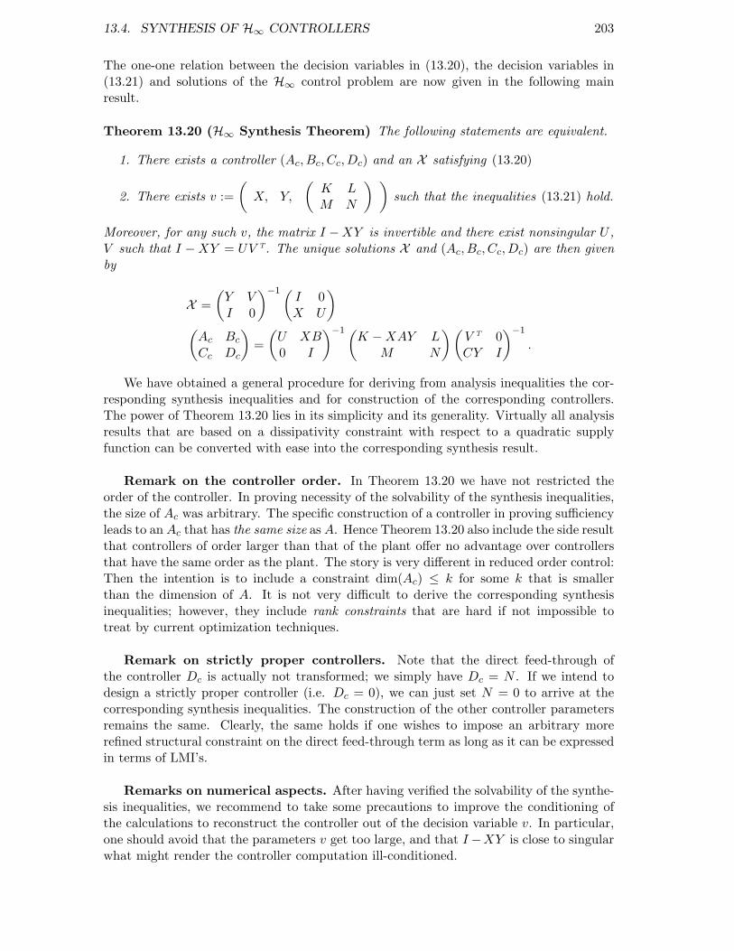
13.4. SYNTHESIS OF H∞ CONTROLLERS 203
The one-one relation between the decision variables in (13.20), the decision variables in(13.21) and solutions of the H∞ control problem are now given in the following mainresult.
Theorem 13.20 (H∞ Synthesis Theorem) The following statements are equivalent.
1. There exists a controller (Ac, Bc, Cc, Dc) and an X satisfying (13.20)
2. There exists v :=(X, Y,
(K LM N
) )such that the inequalities (13.21) hold.
Moreover, for any such v, the matrix I −XY is invertible and there exist nonsingular U ,V such that I −XY = UV T. The unique solutions X and (Ac, Bc, Cc, Dc) are then givenby
X =(Y VI 0
)−1(I 0X U
)(Ac Bc
Cc Dc
)=(U XB0 I
)−1(K −XAY L
M N
)(V T 0CY I
)−1
.
We have obtained a general procedure for deriving from analysis inequalities the cor-responding synthesis inequalities and for construction of the corresponding controllers.The power of Theorem 13.20 lies in its simplicity and its generality. Virtually all analysisresults that are based on a dissipativity constraint with respect to a quadratic supplyfunction can be converted with ease into the corresponding synthesis result.
Remark on the controller order. In Theorem 13.20 we have not restricted theorder of the controller. In proving necessity of the solvability of the synthesis inequalities,the size of Ac was arbitrary. The specific construction of a controller in proving sufficiencyleads to an Ac that has the same size as A. Hence Theorem 13.20 also include the side resultthat controllers of order larger than that of the plant offer no advantage over controllersthat have the same order as the plant. The story is very different in reduced order control:Then the intention is to include a constraint dim(Ac) ≤ k for some k that is smallerthan the dimension of A. It is not very difficult to derive the corresponding synthesisinequalities; however, they include rank constraints that are hard if not impossible totreat by current optimization techniques.
Remark on strictly proper controllers. Note that the direct feed-through ofthe controller Dc is actually not transformed; we simply have Dc = N . If we intend todesign a strictly proper controller (i.e. Dc = 0), we can just set N = 0 to arrive at thecorresponding synthesis inequalities. The construction of the other controller parametersremains the same. Clearly, the same holds if one wishes to impose an arbitrary morerefined structural constraint on the direct feed-through term as long as it can be expressedin terms of LMI’s.
Remarks on numerical aspects. After having verified the solvability of the synthe-sis inequalities, we recommend to take some precautions to improve the conditioning ofthe calculations to reconstruct the controller out of the decision variable v. In particular,one should avoid that the parameters v get too large, and that I−XY is close to singularwhat might render the controller computation ill-conditioned.
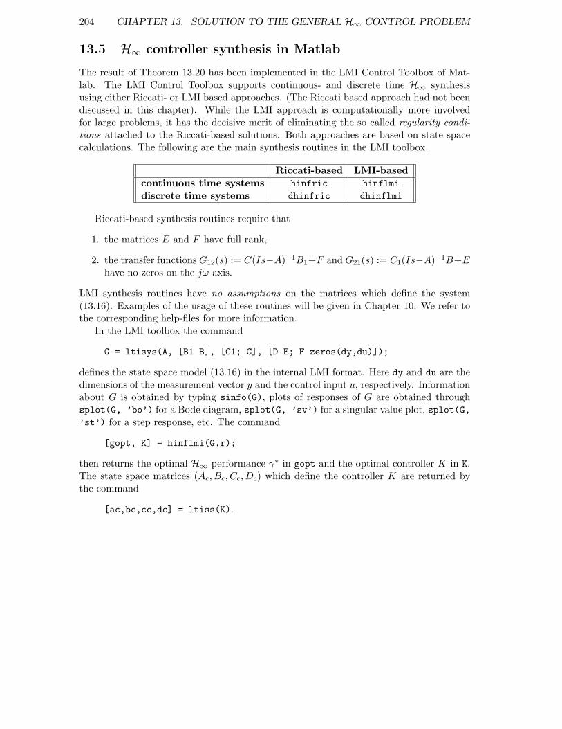
204 CHAPTER 13. SOLUTION TO THE GENERAL H∞ CONTROL PROBLEM
13.5 H∞ controller synthesis in Matlab
The result of Theorem 13.20 has been implemented in the LMI Control Toolbox of Mat-lab. The LMI Control Toolbox supports continuous- and discrete time H∞ synthesisusing either Riccati- or LMI based approaches. (The Riccati based approach had not beendiscussed in this chapter). While the LMI approach is computationally more involvedfor large problems, it has the decisive merit of eliminating the so called regularity condi-tions attached to the Riccati-based solutions. Both approaches are based on state spacecalculations. The following are the main synthesis routines in the LMI toolbox.
Riccati-based LMI-basedcontinuous time systems hinfric hinflmidiscrete time systems dhinfric dhinflmi
Riccati-based synthesis routines require that
1. the matrices E and F have full rank,
2. the transfer functions G12(s) := C(Is−A)−1B1+F and G21(s) := C1(Is−A)−1B+Ehave no zeros on the jω axis.
LMI synthesis routines have no assumptions on the matrices which define the system(13.16). Examples of the usage of these routines will be given in Chapter 10. We refer tothe corresponding help-files for more information.
In the LMI toolbox the command
G = ltisys(A, [B1 B], [C1; C], [D E; F zeros(dy,du)]);
defines the state space model (13.16) in the internal LMI format. Here dy and du are thedimensions of the measurement vector y and the control input u, respectively. Informationabout G is obtained by typing sinfo(G), plots of responses of G are obtained throughsplot(G, ’bo’) for a Bode diagram, splot(G, ’sv’) for a singular value plot, splot(G,’st’) for a step response, etc. The command
[gopt, K] = hinflmi(G,r);
then returns the optimal H∞ performance γ∗ in gopt and the optimal controller K in K.The state space matrices (Ac, Bc, Cc, Dc) which define the controller K are returned bythe command
[ac,bc,cc,dc] = ltiss(K).

Bibliography
[1] J.M. Maciejowski, “Multivariable Feedback Design,” Addison Wesley, 1989.
[2] J. Doyle, B. Francis, A. Tannenbaum, “Feedback Control Theory,” McMillan Publish-ing Co., 1990.
[3] M. Morari, E. Zafiriou, “Robust Process Control,” Prentice Hall Inc., 1989.
[4] B.A. Francis, “A Course in H∞ Control Theory,” Lecture Notes in Control and Infor-mation Sciences, Vol. 88, Springer, 1987.
[5] D.C. Mc.Farlane and K. Glover, “Robust Controller Design using Normalized CoprimePlant Descriptions,” Lecture Notes in Control and Information Sciences, Vol. 138,Springer, 1990.
[6] A. Packard and J. Doyle, “The Complex Structured Singular Value,” Automatica, Vol.29, pp.71–109, January 1993.
[7] A. Weinmann, “Uncertain Models and Robust Control,” Springer, 1991.
[8] I. Postlethwaite, “Robust Control of Multivariable Systems using H∞ Optimization,”Journal A, Vol 32, No. 4, pp 8–19, 1991.
[9] B.Ross Barmish, “New Tools fo Robustness of Linear Systems”, Macmillan PublishingCompany,1994.
[10] Doyle and Stein,“Robustness with Observers”, IEEE AC-24, no.4, August 1997.
[11] G.Zames and B.A.Francis,“Feedback ,Minimax Sensitivity and Optimal Robust-ness”,IEEE AC-28,no.5,May 1983.
[12] M. Green and D.J.N. Limebeer, “Linear Robust Control”, Prentice Hall Informationand System Science Series, New Yersey, 1995.
[13] S.P. Bhattacharyya, H. Chapellat and L.H. Keel, “Robust Control: The ParametricApproach ”,Prentice Hall Information and Science Series, New Yersey, 1995.
[14] K. Zhou, with J.C. Doyle and K. Glover,“Robust and Optimal Control,” PrenticeHall Information and Science Series, New Yersey,1996.
[15] S. Skogestad and I. Postlethwaite,“Multivariable Feedback Control,” John Whileyand Sons, Chichester, 1996.
[16] S. Engell, “Design of Robust Control Systems with Time-Domain Specifications”,Control Eng. Practice, Vol.3, No.3, pp.365-372, 1995.
205

206 BIBLIOGRAPHY
[17] D.F. Enns, “Structured Singular Value Synthesis Design Example: Rocket Stabilisa-tion”, American Control Conf., Vol.3, pp.2514-2520, 1990.
[18] M.A. Peters and A.A. Stoorvogel, “Mixed H2/H∞ Control in a Stochastic Frame-work,” Linear Algebra and its Applications, Vol. 205-206, pp. 971-996, 1984.
[19] S.G. Smit, “Pole-zero cancellations in the multivariable mixed sensitivity problem.”,Selected Topics in Modelling, Identification and Control, Delft University, 1990.


![Robust Control - 東京工業大学CS98] R. Y. Chiang and M. G. Safonov, Robust Control Toolbox User’s Guide, The MathWorks, 1998. 2 HiMAT: Attitude and flight path control 6.86m](https://static.fdocument.pub/doc/165x107/5ad104947f8b9a4e7a8e9aa1/robust-control-cs98-r-y-chiang-and-m-g-safonov-robust.jpg)