
Ostwald Ripening of Droplets: The Role of Migration...
60
Ostwald Ripening of Droplets: The Role of Migration Karl Glasner, Felix Otto, Tobias Rump, Dejan Slepčev no. 339 Diese Arbeit ist mit Unterstützung des von der Deutschen Forschungs- gemeinschaft getragenen Sonderforschungsbereichs 611 an der Universität Bonn entstanden und als Manuskript vervielfältigt worden. Bonn, Mai 2007
Transcript of Ostwald Ripening of Droplets: The Role of Migration...
Ostwald Ripening of Droplets: The Role of Migration
Karl Glasner, Felix Otto, Tobias Rump, Dejan Slepčev
no. 339
Diese Arbeit ist mit Unterstützung des von der Deutschen Forschungs-
gemeinschaft getragenen Sonderforschungsbereichs 611 an der Universität
Bonn entstanden und als Manuskript vervielfältigt worden.
Bonn, Mai 2007
OSTWALD RIPENING OF DROPLETS: THE ROLE OF MIGRATION
KARL GLASNER, FELIX OTTO, TOBIAS RUMP AND DEJAN SLEPCEV
Abstract. A configuration of near-equilibrium liquid droplets sitting on a precursor filmwhich wets the entire substrate can coarsen in time by two different mechanisms: collapseor collision of droplets. The collapse mechanism, i.e., a larger droplet grows at the expenseof a smaller one by mass exchange through the precursor film, is also known as Ostwaldripening.
As was shown by Glasner and Witelski [6] in case of a one-dimensional substrate, themigration of droplets may interfere with Ostwald ripening: The configuration can coarsenby “accidental” collision rather than by collapse. We study the role of migration in caseof a two-dimensional substrate for a whole range of mobilities.
In this paper, we characterize the sign and the scaling of the velocity of a single dropletimmersed into an environment with constant flux field far away. These results allow us –at least for the physically relevant choices for the mobility – to describe the dynamics of adroplet configuration on a two-dimensional substrate by a system of ODEs. In particular,we find by heuristic arguments that collision can be a relevant coarsening mechanism.
1. Introduction
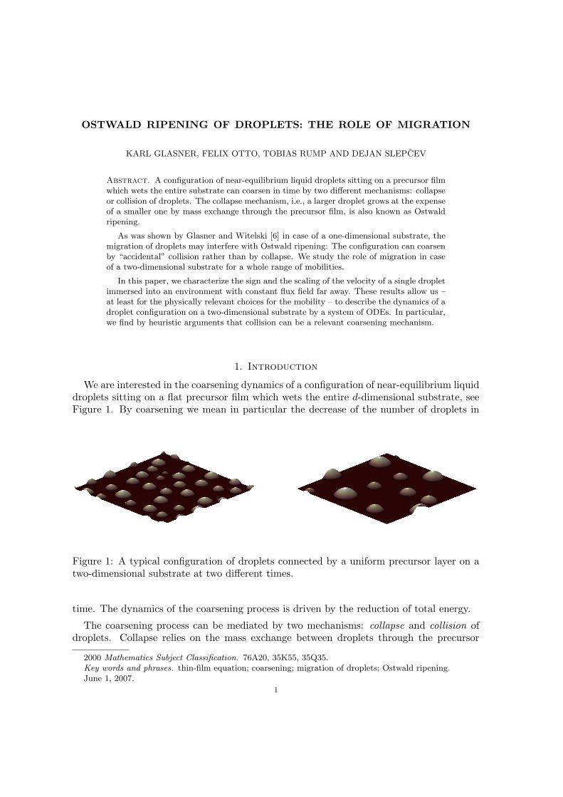
We are interested in the coarsening dynamics of a configuration of near-equilibrium liquiddroplets sitting on a flat precursor film which wets the entire d-dimensional substrate, seeFigure 1. By coarsening we mean in particular the decrease of the number of droplets in
Figure 1: A typical configuration of droplets connected by a uniform precursor layer on atwo-dimensional substrate at two different times.
time. The dynamics of the coarsening process is driven by the reduction of total energy.
The coarsening process can be mediated by two mechanisms: collapse and collision ofdroplets. Collapse relies on the mass exchange between droplets through the precursor
2000 Mathematics Subject Classification. 76A20, 35K55, 35Q35.Key words and phrases. thin-film equation; coarsening; migration of droplets; Ostwald ripening.June 1, 2007.
1
2 KARL GLASNER, FELIX OTTO, TOBIAS RUMP AND DEJAN SLEPCEV
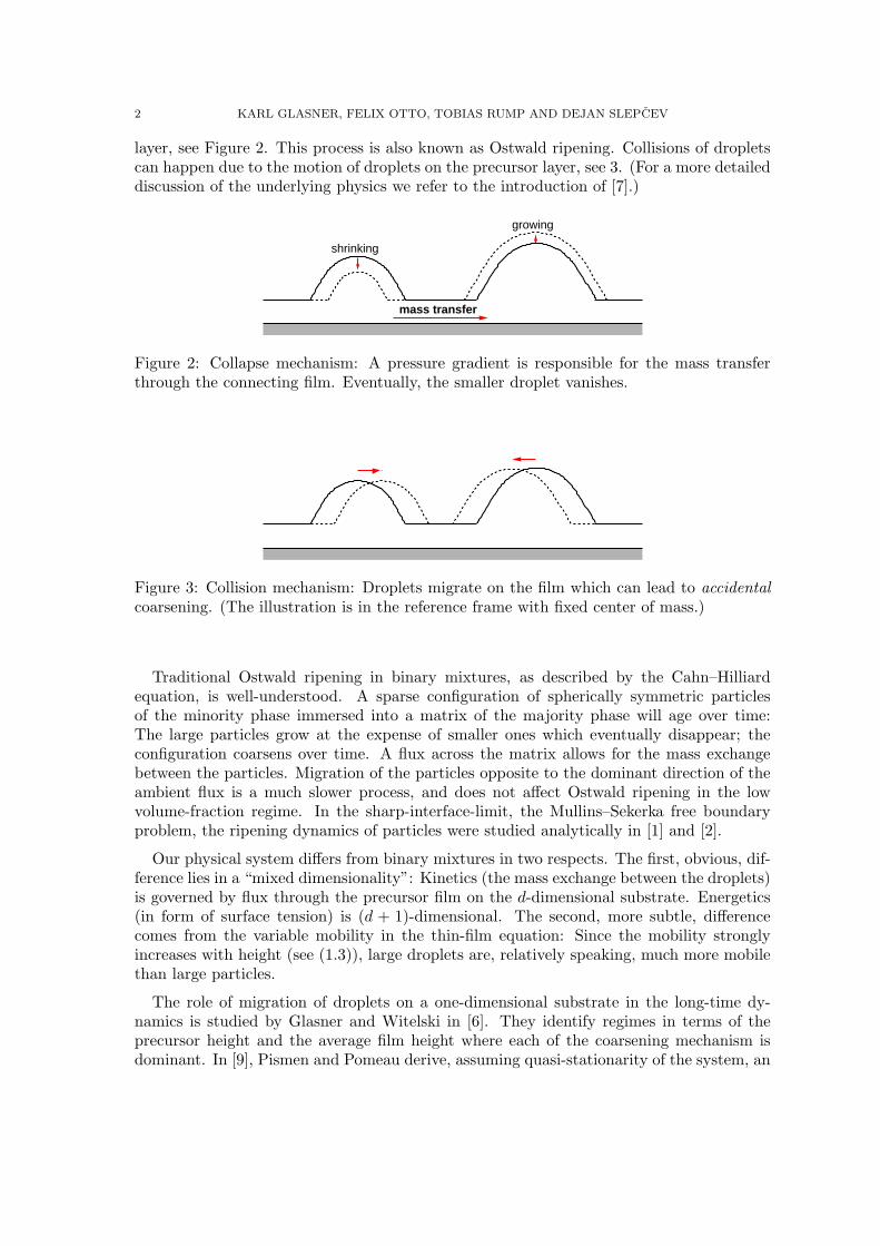
layer, see Figure 2. This process is also known as Ostwald ripening. Collisions of dropletscan happen due to the motion of droplets on the precursor layer, see 3. (For a more detaileddiscussion of the underlying physics we refer to the introduction of [7].)
shrinking
growing
mass transfer
Figure 2: Collapse mechanism: A pressure gradient is responsible for the mass transferthrough the connecting film. Eventually, the smaller droplet vanishes.
Figure 3: Collision mechanism: Droplets migrate on the film which can lead to accidental
coarsening. (The illustration is in the reference frame with fixed center of mass.)
Traditional Ostwald ripening in binary mixtures, as described by the Cahn–Hilliardequation, is well-understood. A sparse configuration of spherically symmetric particlesof the minority phase immersed into a matrix of the majority phase will age over time:The large particles grow at the expense of smaller ones which eventually disappear; theconfiguration coarsens over time. A flux across the matrix allows for the mass exchangebetween the particles. Migration of the particles opposite to the dominant direction of theambient flux is a much slower process, and does not affect Ostwald ripening in the lowvolume-fraction regime. In the sharp-interface-limit, the Mullins–Sekerka free boundaryproblem, the ripening dynamics of particles were studied analytically in [1] and [2].
Our physical system differs from binary mixtures in two respects. The first, obvious, dif-ference lies in a “mixed dimensionality”: Kinetics (the mass exchange between the droplets)is governed by flux through the precursor film on the d-dimensional substrate. Energetics(in form of surface tension) is (d + 1)-dimensional. The second, more subtle, differencecomes from the variable mobility in the thin-film equation: Since the mobility stronglyincreases with height (see (1.3)), large droplets are, relatively speaking, much more mobilethan large particles.
The role of migration of droplets on a one-dimensional substrate in the long-time dy-namics is studied by Glasner and Witelski in [6]. They identify regimes in terms of theprecursor height and the average film height where each of the coarsening mechanism isdominant. In [9], Pismen and Pomeau derive, assuming quasi-stationarity of the system, an
OSTWALD RIPENING OF DROPLETS 3
equation for the droplet motion in an interacting system. We obtain qualitatively differentresults, see Appendix A.
In [7], we studied the statistical behavior of the dynamics characterized by a singlecoarsening exponent and established an upper bound on the coarsening rate. Let us statethat our rigorous result was independent of the question whether migration or Ostwaldripening is the dominant mechanism.
The purpose of this paper is to study the role of migration for the coarsening process interms of the variable mobility in the thin-film equation. We gain the following insights:
• A single droplet in an ambient flux field migrates in the direction of the flux source,i.e. the migration velocity is antiparallel to the flux field, see Figure 6.• The interplay between Ostwald ripening and migration in a many-droplet system
is as follows: The ripening generates an ambient flux field which affects the dropletmigration as in the single-droplet case. Vice versa, migration changes the locationsof the droplets from which the flux stems.• The migration velocity and the volume change can be quantified in terms of scaling
in the droplet size and distance which yield heuristically the typical time scales formigration and Ostwald ripening. The scaling laws depend on the mobility.
The outline of this paper is as follows: The remainder of this section is devoted to thederivation of the thin-film equation. In Section 2, we review the derivation of the equilibriumdroplet profile. The “model problem”, that is, a single near-equilibrium droplet in anambient flux field, is studied in Section 3 where we characterize the migration velocity. Thedetailed analysis related to this section is presented in Section 5 and 6. The interaction ofdroplets in a reduced configuration space is analyzed in Section 4 by means of the Rayleighprinciple. The results (both for one and two dimensions) rely on the analysis of the modelproblem.
1.1. Kinematics, kinetics and energetics.
1.1.1. Kinematics. In the thin-film approximation, the state of the system at time t isdescribed by the film height h = h(x, t) > 0 over a point x ∈ R
d on the substrate. Conser-vation of mass assumes the form of a continuity equation for h:
∂th+∇ · J = 0, (1.1)
where the volume flux J = J(x, t) ∈ Rd is a vector field of the substrate dimension d.
1.1.2. Kinetics. In the thin-film approximation, the flux is generated by the gradient of thepressure µ
J = −m(h)∇µ, (1.2)
where the mobility m is a function of h. The form of the mobility-height relation dependson the underlying (d+ 1)-dimensional fluid model which specifies in particular the bound-ary condition for the fluid velocity at the substrate. For the Stokes equation with no-slipboundary condition, one obtains in the thin-film approximation after suitable nondimen-sionalization
m(h) = h3.
For the Stokes equation endowed with a Navier slip-condition, the mobility is less degener-ate:
m(h) = h2 as long as h � slippage length.
4 KARL GLASNER, FELIX OTTO, TOBIAS RUMP AND DEJAN SLEPCEV
In case of Darcy’s equation with mere no-flux boundary conditions, one ends up with
m(h) = h.
In order to capture the effect of different kinetics, it is convenient to study all homogeneousmobility functions at once:
m(h) = hq for some fixed q ≥ 0. (1.3)
1.1.3. Energetics. We envision a thermodynamically driven situation, where the pressurecomes in form of the functional derivative of a free energy E in the film height:
µ =δE
δh. (1.4)
In our case, the energy is the sum of the surface energy between liquid and vapor and ashort-range interaction potential between substrate, liquid film and vapor (which is onlyeffective where h is sufficiently small):
E(h) =
∫1
2|∇h|2 + U(h) dx, (1.5)
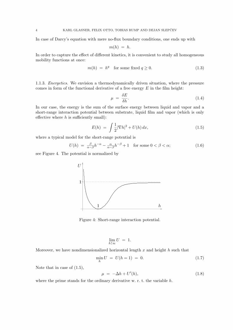
where a typical model for the short-range potential is
U(h) = βα−βh
−α − αα−βh
−β + 1 for some 0 < β < α; (1.6)
see Figure 4. The potential is normalized by
1
1
U
h
Figure 4: Short-range interaction potential.
limh↑∞
U = 1.
Moreover, we have nondimensionalized horizontal length x and height h such that
minhU = U(h = 1) = 0. (1.7)
Note that in case of (1.5),
µ = −∆h+ U ′(h), (1.8)
where the prime stands for the ordinary derivative w. r. t. the variable h.
OSTWALD RIPENING OF DROPLETS 5
1.2. Gradient flow structure and Rayleigh principle. Combining (1.1), (1.2), (1.4),and (1.8), one obtains a nonlinear fourth-order parabolic equation for h:
∂th−∇ ·(m(h)∇(−∆h+ U ′(h))
)= 0. (1.9)
Mathematically speaking, (1.9) is a variant of the Cahn–Hilliard equation if one interprets has the conserved order parameter. The difference to the standard Cahn–Hilliard equation isboth in energetics and kinetics. The difference in energetics is that the nonconvex potentialU is not a “double-well potential” of the universal Ginzburg–Landau type: It only hasa single finite minimum (even when shifted by a linear function). However, the otherminimum can be thought of as h = +∞. The difference in kinetics lies in the fact that themobility m strongly depends on the order parameter. Of course, solution-dependent andeven degenerate mobilities have been considered in the context of the Cahn–Hilliard, see[3] for a mathematical treatment. But the power-law dependence (1.3) together with thefact that the range of h-values is infinite gives rise to new phenomena.
Not surprisingly in view of its derivation, the evolution defined through (1.9) has themathematical structure of a gradient flow – irrespective of the particular form (1.3) of themobility function or the energy (1.5). From a more traditional point of view this meansthat there is a Rayleigh principle: At any time the flux J minimizes
1
2× dissipation rate D + infinitesimal change in energy E.
We note that the viscous dissipation rate is given by
D =
∫1
m(h)|J |2 dx
and according to (1.1) and (1.4), a flux J entails the infinitesimal change in energy
E =
∫δE
δh∂th dx =
∫
µ (−∇ · J) dx =
∫
∇µ · J dx.
Thus at any time, the flux is determined as the minimizer of the Rayleigh functional
1
2
∫1
m(h)|J |2 dx+
∫
J · ∇µdx
=1
2
∫1
m(h)|J |2 dx+
∫
J · ∇(−∆h+ U ′(h)) dx.
One advantage of this formulation is that it separates kinetics (as highlighted by the mo-bility function m(h)) from energetics (as exemplified by the short-range potential U(h)).It uncovers the competition between driving thermodynamics and limiting viscous friction.An immediate consequence of this variational principle is that the minimizer adjusts itselfso that energy balance holds:
E +D = 0.
6 KARL GLASNER, FELIX OTTO, TOBIAS RUMP AND DEJAN SLEPCEV
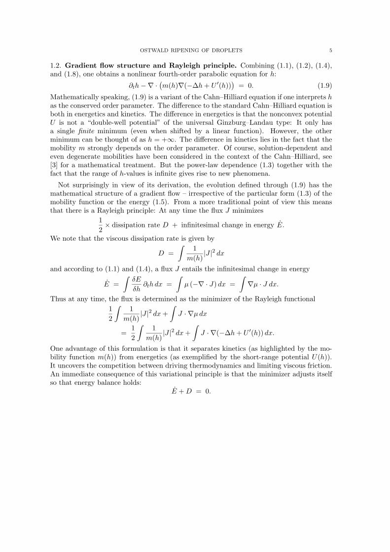
2. Equilibrium droplet
An equilibrium droplet is a stationary point of the energy functional (1.5) subject tothe constraint of constant volume
∫h dx. In view of (1.4) and (1.8), this means that the
pressure is constant:
µ = −∆h+ U ′(h) = const =: P.
droplet center0
1
precursor capfoot
Figure 5: Cross-section of an equilibrium droplet.
We are interested in radially symmetric equilibrium droplets h of asymptotically constantheight h∞ for r = |x−X| ↑ ∞. We focus on the case of a two-dimensional substrate – theone-dimensional substrate is easier. In this case, equilibrium droplets are characterized assolutions of the ODE
−∂2r h− r−1∂rh+ U ′(h) = P,
∂rh(r = 0) = 0 and limr↑∞ h = h∞.(2.1)
Then necessarily U ′(h∞) = P .
We are interested in the regime where 0 < P � 1 and h∞ ≈ 1. We note that to leadingorder,
h∞ − 1 ≈ 1
U ′′(1)P � 1 (2.2)
and thus in particular
U ′′(h∞) ≈ U ′′(1) > 0. (2.3)
We now argue that the droplet profile satisfies
h > h∞ and ∂rh < 0 for r > 0. (2.4)
Indeed, the ODE (2.1) can be interpreted as describing the “position” h as function of“time” r of a particle in the potential V (h) := −(U(h)− Ph) with inertia and friction:
∂2r h+ V ′(h) = −r−1∂rh.
Initially, the particle is at rest: ∂rh(r = 0) = 0. Asymptotically, it reaches h∞, which is alocal maximum of the potential V , cf. (2.3). In view of (1.6), the potential satisfies:
h∞ is the only local maximum of V ,
limh↓0 V = −∞, and limh↑∞ V = +∞.
OSTWALD RIPENING OF DROPLETS 7
Hence the particle can only be to the right of its asymptotic position, which proves thefirst item in (2.4). Furthermore, the particle can only come to rest in finite time on anuphill slope. But then it would be trapped below this V -value and could not reach thelocal maximum h∞. This shows that the particle moves monotonically, the second item in(2.4).
2.1. Precursor, foot and cap region of a droplet. For the convenience of the reader,we reproduce the asymptotic analysis of the solution to (2.1) in the regime P � 1. Thiswill also allow us to refer to some of the arguments and intermediate results later on. Inview of (2.4), there exists a unique radius R > 0 such that
h(r = R) = 2, (2.5)
which we think of as the droplet radius.Precursor region. We first consider the precursor region r ≥ R. Let us neglect the
first order term in (2.1):
−∂2r h+ U ′(h)− U ′(h∞) = 0 for r ≥ R,
and check later that this is to leading order consistent. Because of the boundary conditionin (2.1), we conclude from the above
−1
2(∂rh)
2 +W (h) = 0 for r ≥ R, (2.6)
where
W (h) := U(h)−(U(h∞) + U ′(h∞)(h− h∞)
). (2.7)
From (2.4), (2.5) and (2.6) we obtain∫ 2
h(r)
1√
2W (h)dh = r −R. (2.8)
Since
W (h) ≈ 1
2U ′′(h∞)(h− h∞)2 ≈ 1
2U ′′(1)(h− h∞)2, (2.9)
the integral in (2.8) diverges logarithmically near h = h∞. Hence we have to leading order
ln(h(r)− h∞) =√
U ′′(1) (R− r) for r −R� 1. (2.10)
Thus the droplet height converges exponentially (at order-one rate) to its limiting value asthe distance to the droplet perimeter increases.
The first order term 1r∂rh is indeed negligible with respect to U ′(h)− U ′(h∞) = W ′(h).
In view of (2.6), this follows from
1
R
√
2W (h) � W ′(h) for all h∞ ≤ h ≤ 2. (2.11)
For h close to h∞, both terms scale as h − h∞, cf. (2.9). Thus (2.11) is satisfied providedR� 1. In the end, we shall see that R ∼ P−1 so that this is satisfied.
Foot region. It is convenient to introduce the change of variable
r
R= exp
( s
R
)
(2.12)
for which (2.1) turns into
−∂2s h+ exp(2
s
R)(U ′(h)− U ′(h∞)) = 0 for s ∈ R.
8 KARL GLASNER, FELIX OTTO, TOBIAS RUMP AND DEJAN SLEPCEV
For
| sR| � 1 ⇐⇒ | r
R− 1| � 1, (2.13)
this equation is to leading order approximated by the autonomous equation
−∂2s h+ (U ′(h)− U ′(h∞)) = 0 for | s
R| � 1.
This implies in original variables to leading order
−1
2(∂rh)
2 +W (h) = const for | rR− 1| � 1. (2.14)
Matching function and derivative of (2.6) and (2.14) in the overlap region 0 < r −R� R,we gather that to leading order, the constant in (2.14) must vanish so that in view of (2.5)we have
∫ 2
h(r)
1√
2W (h)dh = r −R for | r
R− 1| � 1. (2.15)
From
W (h) ≈ 1 for 1� h� P−1,
and (2.15) we deduce that to leading order
h(r) =√
2(R− r) for 1� R− r � min{R,P−1}. (2.16)
Cap region. We preliminarily define the cap region as the region where
h � 1 and U ′(h) � P. (2.17)
Based on the form (1.6) of U , (2.17) is equivalent to
h � (P−1)1
β+1 . (2.18)
Because of (2.17), (2.1) is well-approximated by
−∂2r h−
1
r∂rh = P.
Taking into account the left boundary condition in (2.1), all solutions are of the form
h = h(r = 0)− P
4r2. (2.19)
Matching function and derivative of (2.16) and (2.19) yields to leading order
P ≈ 2√
2
Rand h(r = 0) =
R√2. (2.20)
Hence in view of (2.18) the cap region is characterized by
h =R√2
(
1−( r
R
)2)
for R− r � (P−1)1
β+1 . (2.21)
Notice that in the overlap region (P−1)1
β+1 � R − r � P−1, which is nontrivial becauseof β > 0, the functions (2.16) and (2.21) including their derivatives indeed agree to leadingorder.
OSTWALD RIPENING OF DROPLETS 9
Mesoscopic droplet profile. From the above analysis, we learn that there exists anR such that to leading order
R ≈ 2√
2P−1, (2.22)
h =R√2
(
1−( r
R
)2)
for R− r � 1, (2.23)
h = 1 for r −R� 1. (2.24)
Indeed, (2.22) is a reformulation of the first item in (2.20), (2.23) follows from the combi-nation of (2.16) and (2.21), whereas (2.24) is a weakening of (2.10). Thus on a mesoscopiclevel, h is well-described by what we call the mesoscopic droplet profile
hmeso =
R√2
(
1−( r
R
)2)
+ 1 for r ≤ R,1 for r ≥ R
where R = 2
√2P−1. (2.25)
This is not surprising, since hmeso is the radially symmetric minimizer of the mesoscopicenergy functional
Emeso(h) =
∫1
2|∇h|2 + Umeso(h) dx (2.26)
where
Umeso(h) =
{
1 for h > 1,
0 for h ≤ 1.(2.27)
In particular, the apparent contact angle corresponds to a slope of√
2 in our nondimen-sionalization (1.7).
10 KARL GLASNER, FELIX OTTO, TOBIAS RUMP AND DEJAN SLEPCEV
3. Droplet migration
In this section, we analyze the migration of an equilibrium droplet “in vitro”. Thatis, we characterize the migration of a single near-equilibrium droplet in an ambient fluxfield; see Figure 6. Our analysis is motivated by the findings of Glasner in Witelski [5, 6]for one-dimensional substrates. Our goal is to characterize how the “response” of thedroplet depends on its radius R. Our main effort is targeted towards a two-dimensionalsubstrate. For comparison, we treat the much easier case of a one-dimensional substratein the Appendix. It turns out that, at least in terms of scaling in R, the two-dimensionalcase does not differ from the one-dimensional case.
As we shall see, the scaling of the response in R depends on the exponent q in the mobilityfunction, cf. (1.3). The values of q = 3 (not surprisingly) and q = 2 (more surprisingly)play a special role. For q < 2, the variable mobility does not affect the propensity of thedroplet to migrate. On the other hand, starting from q > 3, the effect of variable mobilitysaturates.
We give now a summary of this section. In Subsection 3.1, we introduce the setup of anear-equilibrium droplet immersed into an ambient flux field. We implicitly characterize themigration velocity by the Rayleigh principle and by a solvability condition. In Subsection3.2, we derive a semi-explicit formula for the migration velocity. It involves the solutionof two auxiliary problems for pressures ψ0 and ψ1. We also argue that the droplet alwaysmigrates opposite to the flux imposed far away. In Subsection 3.3, we state our results onthe scaling of the migration speed in the droplet radius R � 1. The detailed analysis ispresented in Sections 5 and 6, where we characterize the solutions ψ1 and ψ0, respectively,of the two auxiliary problem introduced in Subsection 3.2. For ψ1, we use arguments whichcould be made rigorous in the framework of Γ-convergence. For ψ0, we use conventionalasymptotic analysis.
In Appendix A, we compare the migration of a droplet in a flux field to the sliding of adroplet in an external potential. The latter situation was analyzed by Pismen and Pomeau[9], but we obtain different results.
3.1. Set-up for migration. We want to characterize the migration speed of a near-equilibrium droplet immersed into an environment with prescribed constant flux J∞ faraway from the droplet. We let X denote the center of mass of the droplet and write
r = |x−X| and ν =x−Xr
.
We claim that the migration speed X of the droplet, together with the flux field J , ischaracterized by the following problem:
−X · ∇h−∇ · (m∇µ) = 0, (3.1)
J · ν → J∞ · ν as r ↑ ∞ where J := −m∇µ, (3.2)∫
µ∇h dx = 0. (3.3)
We think of (3.1) as an elliptic equation for the pressure µ endowed with the flux boundaryconditions (3.2). Here and in the sequel, m := m(h) denotes the space-dependent mobilityfunction for the equilibrium droplet shape h.
We shall give two arguments in favor of (3.1), (3.2) and (3.3). The first is based on theRayleigh principle, cf. Subsection 1.2, the second one on a solvability argument. By the
OSTWALD RIPENING OF DROPLETS 11
Rayleigh principle, the flux J and the migration speed X minimize as a couple the totaldissipation rate D
1
2D =
1
2
∫1
m|J |2 dx, (3.4)
subject to the continuity equation
−X · ∇h+∇ · J = 0 (3.5)
endowed with the boundary condition
J · ν → J∞ · ν as r ↑ ∞.Hence the droplet migrates in order to minimize the overall dissipation rate under the fluxboundary condition, which is a purely kinetic effect.
The variation in J yields that J is of the form
J = −m∇µ, (3.6)
so that (3.5) turns into (3.1). Since (3.5) can be formulated as
∇ · (−X (h− h∞) + J) = 0, (3.7)
the variation of (3.4) w. r. t. X yields (3.3):
0 =
∫1
m(h− h∞) J dx
(3.6)= −
∫
(h− h∞)∇µdx =
∫
µ∇h dx. (3.8)
We now argue that (3.3) can also be interpreted in a more traditional way as solvabilitycondition. We are interested in a solution of the thin-film equation, which we rewrite as
∂th−∇ · (m(h)∇µ) = 0, (3.9)
µ = −∆h+ U ′(h), (3.10)
endowed with the flux boundary conditions
J := −m(h)∇µ → J∞ as |x−X| ↑ ∞.We seek a solution of the form
h = h(x−X(t)) + h1(t, x), (3.11)
where we think of h1 as a perturbation of the equilibrium droplet profile h. The latter ischaracterized by
−∆h+ U ′(h) = U ′(h∞), (3.12)
cf. Section 2. Notice that (3.12) implies (a consequence of translational invariance)
−∆∇h+ U ′′(h)∇h = 0. (3.13)
In view of (3.12), up to the order of the perturbation (3.10) is
µ = U ′(h∞)−∆h1 + U ′′(h)h1. (3.14)
Testing (3.14) with the exponentially decaying ∇h yields (3.3):∫
µ∇h dx (3.14)=
∫
(−∆h1 + U ′′(h)h1)∇h dx
=
∫
h1 (−∆∇h+ U ′′(h)∇h) dx (3.13)= 0. (3.15)
On the other hand, (3.11) inserted into (3.9) yields (3.1) to leading order. Indeed, wemay replace m(h) by its leading order m(h) = m since µ = U ′(h∞) = const to leading
12 KARL GLASNER, FELIX OTTO, TOBIAS RUMP AND DEJAN SLEPCEV
order, cf. (3.14). A broader analogy to systematic asymptotic expansions is described inthe Appendix.
3.2. Characterization and sign of the migration velocity. The problem (3.1), (3.2)and (3.3) defines a linear relationship between the flux at infinity, J∞, and the droplet
migration speed X, which we want to characterize more explicitly.
We consider the 1-d substrate in the Appendix B.1. For a 2-d substrate, we introducetwo auxiliary problems: Let ψ0 denote the solution of the homogeneous equation withinhomogeneous boundary conditions, that is,
−∇ · (m∇ψ0) = 0,
J0 · ν →(10
)· ν as |x| ↑ ∞ where J0 := m∇ψ0
(3.16)
(note the change of sign in the definition of J0, which is convenient for later purposes) andψ1 the solution of the inhomogeneous equation with homogeneous boundary conditions, i.e.
−∂1h−∇ · (m∇ψ1) = 0,
J1 · ν → 0 as |x| ↑ ∞ where J1 := −m∇ψ1,(3.17)
Notice that both auxiliary problems allow for a physical interpretation: Problem (3.16)determines the pressure −ψ0 which arises from a nonzero flux-boundary condition at infinityin a locally perturbed environment described by a variable mobility m. Problem (3.17)determines the pressure ψ1 which is necessary to make the equilibrium droplet migrate atunit speed. From (3.1) and (3.2) we read off that µ must be of the form
µ = −J∞ ψ0 + X ψ1.
Here and in the sequel, we invoke isotropy to identify the vectors J∞ and X with the scalars
in(J∞0
)and
(X0
)respectively. Hence (3.3) turns into
X =
∫ψ0 ∂1h dx
∫ψ1 ∂1h dx
J∞. (3.18)
Let us argue how the 2-d formula (3.18) relates to the 1-d formula (B.1). Substituting∂1h in (3.18) according to (3.17) and formally integrating by parts yields
X =
∫m∇ψ0 · ∇ψ1 dx∫m∇ψ1 · ∇ψ1dx
J∞ = −∫
1mJ0 · J1 dx∫
1m |J1|2 dx
J∞. (3.19)
On a 1-d substrate, (3.19) coincides with (B.1) since then, the solution of (3.16) is J0 ≡ 1and that of (3.17) is J1 = h− h∞.
However, the integration by parts is only allowed in the denominator of (3.19). Indeed,since h depends only on r = |x−X|, it is convenient to introduce polar coordinates
x−X =
(r cosϕ
r sinϕ
)
.
In this notation, both ψ0 and ψ1 are of the form
ψi(x) = ψi(r) cosϕ, (3.20)
OSTWALD RIPENING OF DROPLETS 13
(it will always be clear from the context whether we mean ψi(x) or ψi(r)) where thefunctions ψi(r) are determined by
−∂r(m∂rψ0)− mr ∂rψ0 + m
r2ψ0 = 0,
ψ0(r = 0) = 0, limr↑∞ ∂rψ0 = 1,(3.21)
and−∂r(h− h∞)− ∂r(m∂rψ1)− m
r ∂rψ1 + mr2ψ1 = 0,
ψ1(r = 0) = 0, limr↑∞ ∂rψ1 = 0,(3.22)
respectively. We also recall that up to exponentially small terms, the film height is constantin the precursor film:
h = h∞ for r −R � 1,
where R denotes the mesoscopic droplet radius, cf. Section 2. Hence in particular thecoefficient m is constant there:
m∞ = const for r −R � 1.
Since {r, r−1} is a fundamental system of the constant coefficient ODE −∂2− r−1∂r + r−2,we infer the following form of the solutions of (3.21) and (3.22) in the precursor film
ψ0 = r + const
r
ψ1 = const
r
}
for r −R� 1. (3.23)
This asymptotic behavior justifies the integration by parts of the denominator in (3.18):∫
ψ1 ∂1(h− h∞) dx = −∫
ψ1∇ · (m∇ψ1) dx =
∫
m|∇ψ1|2 dx,
but shows that the numerator in (3.18) has to be kept as is:
X =
∫ψ0 ∂1h dx
∫m |∇ψ1|2 dx
J∞, (3.24)
or in polar coordinates
X =
∫∞0 ψ0 ∂rh r dr
∫∞0 m ((∂rψ1)2 + r−2ψ2
1) r drJ∞.
The factor which relates X to J∞ has the same sign as for 1-d substrates:∫∞0 ψ0 ∂rh r dr
∫∞0 m ((∂rψ1)2 + r−2ψ2
1) r dr< 0.
In particular, the droplet in the ambient flux field J∞ migrates in opposite direction; seeFigure 6.
Indeed, we have on the one hand
∂rh ≤ 0 for r > 0,
and on the other hand
ψ0 > 0 for all r > 0. (3.25)
The latter can be obtained as follows: Notice that (3.23) yields in particular that ψ0 ≥ 0for sufficiently large r. Together with ψ0(r = 0) = 0 we infer from the maximum principlefor −∂rm∂r − r−1m∂r + r−2m that
ψ0 ≥ 0 for all r ≥ 0. (3.26)
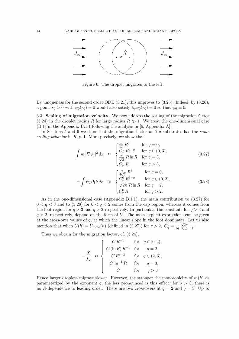
14 KARL GLASNER, FELIX OTTO, TOBIAS RUMP AND DEJAN SLEPCEV
XJ∞ J∞
Figure 6: The droplet migrates to the left.
By uniqueness for the second order ODE (3.21), this improves to (3.25). Indeed, by (3.26),a point r0 > 0 with ψ0(r0) = 0 would also satisfy ∂rψ0(r0) = 0 so that ψ0 ≡ 0.
3.3. Scaling of migration velocity. We now address the scaling of the migration factor(3.24) in the droplet radius R for large radius R � 1. We treat the one-dimensional case(B.1) in the Appendix B.1.1 following the analysis in [6, Appendix A].
In Sections 5 and 6 we show that the migration factor on 2-d substrates has the same
scaling behavior in R� 1. More precisely, we show that
∫
m |∇ψ1|2 dx ≈
π12 R
4 for q = 0,
C1q R
4−q for q ∈ (0, 3),π√2R lnR for q = 3,
C1q R for q > 3,
(3.27)
−∫
ψ0 ∂1h dx ≈
π4√
2R3 for q = 0,
C0q R
3−q for q ∈ (0, 2),√2π R lnR for q = 2,
C0q R for q > 2.
(3.28)
As in the one-dimensional case (Appendix B.1.1), the main contribution to (3.27) for0 < q < 3 and to (3.28) for 0 < q < 2 comes from the cap region, whereas it comes fromthe foot region for q > 3 and q > 2 respectively. In particular, the constants for q > 3 andq > 2, respectively, depend on the form of U . The most explicit expressions can be givenat the cross-over values of q, at which the linear slope in the foot dominates. Let us also
mention that when U(h) = Umeso(h) (defined in (2.27)) for q > 2, C0q =
√2π
(q−2)(q−1) .
Thus we obtain for the migration factor, cf. (3.24),
− X
J∞≈
C R−1 for q ∈ [0, 2),
C (lnR)R−1 for q = 2,
C Rq−3 for q ∈ (2, 3),
C ln−1R for q = 3,
C for q > 3
Hence larger droplets migrate slower. However, the stronger the monotonicity of m(h) asparameterized by the exponent q, the less pronounced is this effect; for q > 3, there isno R-dependence to leading order. There are two cross-overs at q = 2 and q = 3: Up to
OSTWALD RIPENING OF DROPLETS 15
q = 2, the scaling of the response is independent of q, and starting from q = 3, the scalingexponent saturates.
Let us also remark here that the quantity in (3.28) and the asymptotic behavior of ψ1
are related: We claim that
limr→∞
rψ1(r) =1
2π
∫
R2
ψ0 ∂1h dx. (3.29)
To show that consider r � L. Integrating by parts twice yields∫
B(0,r)∇ · (m∇ψ1)ψ0 dx−
∫
B(0,r)ψ1∇ · (m∇ψ0) dx
=
∫
∂B(0,r)m ψ0∇ψ1 ·
x
|x| dx−∫
∂B(0,r)m ψ1∇ψ0 ·
x
|x| dx.
Using (3.16) and (3.17) we obtain
−∫
B(0,r)∂1hψ0 dx =
∫ 2π
0ψ0(r)∂rψ1(r) cos2 θ r dθ −
∫ 2π
0ψ1(r)∂rψ0(r) cos2 θ r dθ.
Using the asymptotic behavior of ψ0(r) and ψ1 obtained in (3.23)
ψ0(r) ≈ r, ∂rψ0(r) ≈ 1 ∂rψ1(r) ≈ −1
rψ1(r) as r →∞.
by taking the limit r →∞ we obtain
−∫
R2
ψ0 ∂1h dx = −2π limr→∞
rψ1(r). (3.30)
16 KARL GLASNER, FELIX OTTO, TOBIAS RUMP AND DEJAN SLEPCEV
4. Interacting mesoscopic droplets
While in the previous section we considered how a single droplet interacts with an am-bient flux field, here we are interested how droplets interact with each other. In particularwe are interested in the regime of large, quasi-stationary, well-separated droplets. That is,
1 � R ∼ V 1
d+1 � L, (4.1)
where R is the typical radius, V the typical volume of a droplet, and L is the typicaldistance between droplets (defined as (number density of droplets)−1/d).
We impose the quasi-stationarity of the system by reducing the configuration space tocollections of stationary droplets. The stationary droplets have slightly different heights inthe tail region; the discrepancy is comparable to 1/R. In the case that the excess mass inthe precursor is small compared to the droplet mass, that is when R2 � L, the variationof the height in the precursor layer does not have an effect on the leading order dynamics.In our setup one could deal with discrepancies in the tail region by smoothly replacing thetails by constant height 1 beyond some intermediate distance, d, (R� d� L).
However, we choose to deal with the tails by introducing a further reduction. Thatis, we study the system on the mesoscopic level. We reduce the configuration space tothe mesoscopic shape of the droplets (2.23), that is to parabolic droplets of fixed contactangle on the precursor layer. Hence the configuration is fully described by the centers andvolumes of the droplets.
The dynamics of the interacting droplets is determined by the Rayleigh principle, de-scribed in Subsection 1.2. That is, at any time the flux J (subject to the continuityequation) minimizes
12D + E.
On the reduced configuration space we consider the mesoscopic energy (2.26)
E(h) = Emeso(h) =
∫
12 |∇h|2 + Umeso(h) dx, (4.2)
for which the parabolic droplets are exact steady states, see (2.25). We choose this reductionas it enables us to make the presentation simple and transparent.
The analysis of the previous section and that of ψ0 and ψ1 in Sections 5 and 6 shows thatfor q ≤ 2 the interaction of large droplets with their environment depends to leading orderonly on the mesoscopic profile, and not on the details of the potential U . In particular, theasymptotic values of the quantities in (3.27) and (3.28) rely only on the mesoscopic shapeof the droplet. For q > 2 the dependence on the particular form of U is only through aU -dependent constant factor. Thus even though our reduced system neglects the preciseshape of the droplet, the reduced dynamics differs from the actual limiting dynamics in thecase of q > 2 only by a constant factor in the migration terms; see (4.25) and (4.26).
We present the analysis only for the 2-d systems in detail. The analysis is not fullyrigorous as it depends on conclusions of asymptotic analysis of Sections 5 and 6. We dohowever validate the smallness of the lower order terms in the approximations we carryout. Results of the 1-d analysis are given in Appendix B. They are in agreement with theconclusions of Glasner and Witelski [5, 6], who already studied the 1-d case with (different)asymptotic tools.
4.1. Reduced structure. In the following, we will introduce the reduced configurationspace and the dynamical structure for both one and two dimensions.
OSTWALD RIPENING OF DROPLETS 17
Configuration space. The parabolic droplets, which are steady states of the mesoscopicenergy (4.2), are parameterized by their volume V (above the precursor height) and centerof mass X:
hV,X(x) := max{
0,− 1√2ωV − 1
d+1 |x−X|2 + 1√2ω V
1
d+1
}
, (4.3)
where
ω :=
(3
2√
2
) 1
2
for d = 1,√
2π−1
3 for d = 2.
The constant ω is chosen such that the radius R and the volume V are related by
R = ω V1
d+1 .
A configuration of n droplets is fully described by the position vector (XT1 , . . . , X
Tn )T with
Xi ∈ Rd and the volume vector (V1, . . . , Vn)
T . We define
hi(x) := hVi,Xi(x),
hΘ(x) := 1 +n∑
i=1
hi(x), Θ := (V1, . . . , Vn, XT1 , . . . , X
Tn )T
and the droplet distances Lij := |Xi −Xj |.An infinitesimal change of a configuration Θ is described by the infinitesimal change of
the droplet volumes and their centers, denoted by Θ:
Θ := (V1, . . . , Vn, XT1 , . . . , X
Tn )T ∈ R
(d+1)n.
Due to the conservation of mass the change vector Θ is admissible, if∑n
i=1 Vi = 0, or in
other words, if Θ is orthogonal to
p = 1√n(1n, 0dn)
T .
(Here we use the notation zk := (z, . . . , z) ∈ Rk, for z ∈ {0, 1}.) The infinitesimal change
of the height profile hΘ of the configuration corresponding to the change vector Θ is givenby
4hΘ :=d
ds
∣∣∣∣s=0
hΘ+sΘ =n∑
i=1
∂hi∂Vi
Vi −∇hi · Xi,
where∂hi∂Vi
:=∂hV,Xi
∂V
∣∣∣∣V=Vi
= 1√2(d+1)ω
V− d+2
d+1
i |x−Xi|2 + 1√2(d+1)
ω V− d
d+1
i (4.4)
for x ∈ B(Xi, Ri).
Energy. On the restricted configuration space the energy has a simple form:
E(hΘ) =√
2(d+1)ω
n∑
i=1
Vd
d+1
i . (4.5)
Note that we skip the subscript “meso” for convenience. The infinitesimal change of energygenerated by the infinitesimal change of the configuration in the direction of Θ is
E[Θ] = ∇E · Θ =√
2dω
n∑
i=1
V− 1
d+1
i Vi.
18 KARL GLASNER, FELIX OTTO, TOBIAS RUMP AND DEJAN SLEPCEV
4.1.1. Reduced Rayleigh dynamics. Analogous to the simpler model problem in the previoussection, see equations (3.4) and (3.5) in 3.1, the trajectory Θ(t) of the system is determined
by the fact that the change vector Θ along with the flux J minimize as a pair the quantity
12D +∇E · Θ
subject to
4hΘ +∇ · J = 0.
The viscous dissipation rate is, as before, quadratic in J : D =∫
1m |J |2 dx.
We already know that the minimizing flux is a gradient of a pressure, that is
J = −m∇ϕΘ,
subject to
4hΘ −∇ · (m∇ϕΘ) = 0.
Consequently to determine Θ one needs to minimize
12
∫
m|∇ϕΘ|2dx+∇E · Θ. (4.6)
Approximately (at least in the sense, that the associated quadratic form of minimaldissipation, i.e. D =
∫m |∇ϕΘ|2 dx, is well-approximated in terms of the following model
pressures as we will see later), the pressure ϕΘ is a linear combination of the following“decoupled” ones:
• Pressure relevant to droplet motion: We recall the two auxiliary problems (3.16)and (3.17) in a slightly modified form. We introduce the pressures Ψ0,V (generatedby a nonzero flux-boundary condition far from droplet) by
−∇ · (m∇Ψ0,V ) = 0,
J0,V · ν →(10
)· ν as |x| ↑ ∞, where J0,V := m∇Ψ0,V ,
(4.7)
and Ψ1,V , which makes the droplet move with unit speed, by
−∂1hV,0 −∇ · (m∇Ψ1,V ) = 0,
J1,V · ν → 0 as |x| ↑ ∞, where J1,V := −m∇Ψ1,V .(4.8)
As before, m = m(1+hV,0). The subscript V highlights the dependence of m and hon the volume. Note that both Ψ0,V and Ψ1,V are centered in the origin in contrastto the pressures determined by (3.16) and (3.17). Furthermore we use explicitly themesoscopic droplet profile for the characterization.
Using the isotropy of the mobility in (4.8) we can determine the pressure corre-
sponding to arbitrary droplet velocity vector X ∈ R2 instead of (1, 0)T . We denote
this pressure by ΨX1,V . It has a dipolar form:
ΨX1,V (x) = Ψ1,V (|x|) |X| cos θ (4.9)
in the polar coordinates determined by
x
|x| ·X
|X|= cos θ.
OSTWALD RIPENING OF DROPLETS 19
• Pressure relevant to droplet mass change: We introduce the pressure needed tomove the mass from a single mesoscopic droplet into the surrounding precursorfilm: ΨV is a radially symmetric solution of
∇ · (m∇ΨV ) = −∂hV,0∂V
. (4.10)
Note that outside of the droplet ΨV satisfies the Laplace equation. For r > R,where R = ωV 1/3 is the radius of the droplet, we have
1 =
∫
B(0,r)
∂hV,0∂V
dx = −∫
∂B(0,r)m∇ΨV · ν = −2πr(∂rΨV ).
Therefore we can determine the pressure outside of the droplet up to an additiveconstant
ΨV (x) = − 1
2πln |x|+ const. for |x| > R. (4.11)
Since ϕΘ depends linearly on the change Θ, the first term in (4.6) defines a quadratic
form in Θ. The associated bilinear form is
D(Θ, Ξ) :=
∫1
mJΘ · JΞ dx =
∫
m∇ϕΘ · ∇ϕΞ dx (4.12)
for admissible change vectors Θ and Ξ. Since the space of admissible change vectors isfinite-dimensional, there is a symmetric matrix G representing the bilinear form:
ΘTG Ξ = D(Θ, Ξ).
Such matrix G is not unique. The canonical choice is the matrix G which also satisfiesGp = 0. A symmetric matrix G represents the same bilinear form on the set of admissiblechange vectors if and only if ΠGΠ = G, where Π = I − ppT is the orthogonal projection tothe orthogonal complement of p.
Minimizing (4.6) in the form ΘTGΘ +∇E · Θ in Θ with the constraint Θ · p = 0 gives
that Θ is uniquely determined by
Π(GΘ +∇E) = 0
Θ · p = 0.(4.13)
In the following subsections, we will give asymptotic expressions for the entries of G interms of the auxiliary pressures ΨV and Ψi,V and solve the problem explicitly for a two-droplet-configuration.
4.2. Coefficients of G in the two-dimensional case. As indicated above, the coef-ficients of G describe the dissipation generated by the fluxes that correspond to volumechanges and motion of droplets. For clarity, we subdivide the matrix G ∈ R
3n×3n into threesub-matrices: the volume change matrix Gv ∈ R
n×n, the migration matrix Gm ∈ R2n×2n
and the coupling matrix C ∈ R2n×n:
G =
[Gv CT
C Gm
]
. (4.14)
20 KARL GLASNER, FELIX OTTO, TOBIAS RUMP AND DEJAN SLEPCEV
4.2.1. Approximate coefficients of G . We show in Subsection 4.3 that
Gvij =
{
−12
(∫
B(0,L)m|∇ΨVi|2 +
∫
B(0,L)m|∇ΨVj|2)
+O(1) if i 6= j,
0 if i = j,(4.15)
Gmij =
{
diag(gi, gi) + o(gi)2×2 if i = j,
o(√gigj)2×2 else,
(4.16)
where o(f)2×2 =
[o(f) o(f)o(f) o(f)
]
and
gi =
∫
mi(x) |∇Ψ1,Vi(x)|2 dx, (4.17)
where mi(x) := m(1 + hi(x +Xi)) and Ψ1,Viis defined in (4.8). The coupling coefficients
are given by
Cij =
{Xi−Xj
|Xi−Xj | cij + o(cij)2×1 if i 6= j,
0 else,(4.18)
where, using (3.30)
cij =1
2π
1
|Xi −Xj |
∫
∂1hi(x+Xi) Ψ0,Vi(x)dx =
1
|Xi −Xj |limr→∞
r Ψ1,Vi(r) (4.19)
and Ψ0,Viis defined in (4.7).
Asymptotic values of relevant quantities. Let Lij = |Xi − Xj |. We consider the regimemini6=j Lij � maxiRi. In Subsection 4.3 we show that for i 6= j
Gvij = − 1
4π
(
ln(Lij/V1
3
i ) + ln(Lij/V1
3
j )
)
+O(1).
The asymptotic values of gi and cij for i, j = 1, 2 and i 6= j follow from (3.27) and (3.28):
gi =
C V4−q3
i for q ∈ [0, 3),
π23
3 V1
3
i lnVi for q = 3,
C V1
3
i for q > 3,
(4.20)
cij = − 1
Lij
C V3−q3
i for q ∈ [0, 2),
1
3π43
V1
3
i lnVi for q = 2,
C V1
3
i for q > 2.
(4.21)
OSTWALD RIPENING OF DROPLETS 21
Rayleigh dynamics of two droplets. As an insightful illustration we consider the particularcase of two droplets in detail. Let us compute the equations for Θ in the natural coordinatesfor the two-droplet configuration [e1, e2]:
e1 =X2 −X1
|X2 −X1|, e2⊥e1, |e2| = 1 (4.22)
The characterization of G given in (4.15)-(4.19) yields
G =
0 Gv12 0 0 c21 0Gv12 0 −c12 0 0 00 −c12 g1 0 0 00 0 0 g1 0 0c21 0 0 0 g2 00 0 0 0 0 g2
.
We obtain that the dynamics according to (4.13) is given by the following system of ODEs:
V1 + V2 = 0,
−Gv12V1 +Gv21V2 + c12X11 + c21X
12 = −2
√2
ω(V
− 1
3
1 − V − 1
3
2 ),
g1X11 − c12V2 = 0,
X21 = 0,
g2X12 + c21V1 = 0,
X22 = 0.
Solving the system yields in particular
V1 =2√
2
ω
(
2Gv12 +c212g1
+c221g2
)−1
(V− 1
3
1 − V − 1
3
2 ). (4.23)
Using (4.20) and (4.21), the assumption L12 � V1
3
i for i = 1, 2 yields
−Gv12 � 1� c212gi. (4.24)
Therefore the system of ODEs in the limit reduces to
V1 = − 4π4
3
ln(L/V1
3
1 ) + ln(L/V1
3
2 )(V
− 1
3
1 − V − 1
3
2 ), (4.25)
X11 = −c12
g1V1, X1
2 = −c21g2V1. (4.26)
The equations (4.26) for the motion of the droplets provide a nice way of interpreting theconnection between J∞ in the model problem in Section 3 and the case of a configurationof droplets with at least two droplets. For this purpose, consider the equation of motion
22 KARL GLASNER, FELIX OTTO, TOBIAS RUMP AND DEJAN SLEPCEV
(4.13) that is
X1 = − V2
g1C12 =
∫∂1h1 Ψ0,V1
(x−X1) dx∫m1|∇Ψ1,V1
(x−X1)|2 dx
(
− V2
2π
X1 −X2
|X1 −X2|2
)
=
∫∂1h1 Ψ0,V1
(x−X1) dx∫m1|∇Ψ1,V1
(x−X1)|2 dx
(
−∇(
V2
2πln |X1 −X2|
))
,
and compare it to (3.24) in Section 3. It reveals that in the context of a two-dropletsystem, J∞ can be interpreted as the flux at X1 generated by the harmonic potential whichtransports mass V2 out of the droplet centered in X2.
4.2.2. Time scales in the dynamics. To deduce heuristically the typical time scale of Ost-wald ripening and migration from the reduced structure we assume that the typical lengthscales (like the typical droplet radius) exhibit scaling in time. In addition to scaling inV , we consider how the scaling depends on the average film height H, up to logarithmiccorrections. Note that the mass conservation dictates that
HLd = V. (4.27)
Heuristically, these time scales allow us to identify the dominant coarsening mechanism indifferent regimes.
The equation (4.25) describes the mass transfer rate between two droplets. It follows
V ∼ 1
lnVV − 1
3 ,
where we use (4.27). Hence the time scale for ripening is
τrip =V
V= V
4
3 lnV. (4.28)
We expect that L ∼ |X| and thus
L ∼ |Xi| ∼1
lnLV − 1
31
L
V − 1
3 for q ∈ [0, 2),
V − 1
3 lnV for q = 2,
Vq−3
3 for q ∈ (2, 3),1
lnV for q = 3,
1 for q > 3.
(4.29)
Therefore the time scale for migration of droplets,
τmig =L
L∼ 1
HV
4
3 lnV
V1
3 for q ∈ [0, 2),
V13
lnV for q = 2,
V3−q3 for q ∈ (2, 3),
lnV for q = 3,
1 for q > 3.
(4.30)
Note that τmig � τrip if q < 3 and V � 1 which indicates that droplets are nearlystationary. When q = 3 the difference between time scales is only logarithmic in V , whilewhen q > 3 they are comparable. It is also worth noting the scaling in the average filmheight: The importance of motion of droplets grows if the average film thickness is increased.
OSTWALD RIPENING OF DROPLETS 23
4.3. Derivation of the coefficients of G. We present the details of the derivation ofcoefficients of G only for a configuration of two droplets. It contains all the essentialingredients of the derivation with n droplets present, but is significantly easier to present.Accordingly, we consider a configuration of two droplets, Θ = (V1, V2, X
T1 , X
T2 )T . Let
L = |X2 −X1|.
4.3.1. Computing Gv. Consider the general mass exchange given by the change vector v =(V1, V2, 04)
T with V1 + V2 = 0. Then
4hv(x) =∂h1
∂V1(x)V1 +
∂h2
∂V2(x)V2. (4.31)
By the definition of the dissipation rate (4.12) it follows that
Gv11(V1)2 +Gv22(V2)
2 + 2Gv12V1 V2 = vTGv =
∫
R2
m|∇ϕv(x)|2 dx,
where
∇ · (m∇ϕv) = 4hv. (4.32)
The above condition fully determines the volume exchange part of the bilinear form, D, but,as we discussed before, the matrix G is not unique. Since we have in mind the dissipationdue to mass exchange it is natural to choose G for which Gv
11 = Gv22 = 0, which implies
2Gv12 V1V2 =
∫
R2
m|∇ϕv(x)|2 dx.
To determine the value on the right hand side, we will show that ϕv is, in a sense, well ap-proximated by −V1ΨV1
( · −X1)− V2ΨV2( · −X2). We start by observing that an elementary
computation based on (4.11) shows that for i = 1, 2∫
B(0,L)\B(0,Ri)m|∇ΨVi
|2dx =1
2πln(L/V
1
3
i ) +O(1). (4.33)
Let us now show that the integral over B(0, Ri) is of size O(1). Consider Ji(x) :=
−m(x)∇ΨVi(x). Then ∇·Ji = ∂h
∂V
∣∣V=Vi
. Let y = x/Ri. Let J(y) be the radially symmetric
solution of ∇y · J(y) = ∂h∂V
∣∣V=1
. The scaling property of the family of steady states yields
that J(y) = Ri Ji(x). Therefore∫
B(0,Ri)m|∇ΨVi
|2 ≤∫
B(0,Ri)|Ji(x)|2dx =
∫
B(0,1)|J(y)|2dy, (4.34)
which proves the claim.
Thus we need to show that −2Gv12 = 1
2π (ln(L/V1/31 ) + ln(L/V
1/32 )) + O(1). Note that
there are two representations of∫m|∇ϕv(x)|2 dx:
∫
m|∇ϕv(x)|2 dx = maxζ
{∫
−m|∇ζ(x)|2 + 24hv(x)ζ(x)dx}
(4.35)
= minJ
{∫1
m|J |2dx
∣∣∣ ∇ · J = 4hv
}
. (4.36)
In the following, we provide lower and upper bounds on∫m|∇ϕv(x)|2 dx that differ by an
amount of O(1).
24 KARL GLASNER, FELIX OTTO, TOBIAS RUMP AND DEJAN SLEPCEV
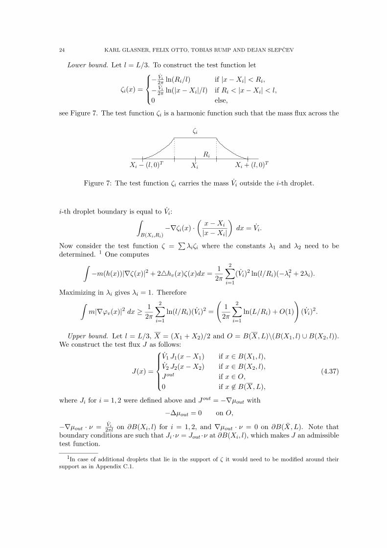
Lower bound. Let l = L/3. To construct the test function let
ζi(x) =
− Vi
2π ln(Ri/l) if |x−Xi| < Ri,
− Vi
2π ln(|x−Xi|/l) if Ri < |x−Xi| < l,
0 else,
see Figure 7. The test function ζi is a harmonic function such that the mass flux across the
ζi
Xi
Ri
Xi − (l, 0)T Xi + (l, 0)T
Figure 7: The test function ζi carries the mass Vi outside the i-th droplet.
i-th droplet boundary is equal to Vi:∫
B(Xi,Ri)−∇ζi(x) ·
(x−Xi
|x−Xi|
)
dx = Vi.
Now consider the test function ζ =∑λiζi where the constants λ1 and λ2 need to be
determined. 1 One computes
∫
−m(h(x))|∇ζ(x)|2 + 24hv(x)ζ(x)dx =1
2π
2∑
i=1
(Vi)2 ln(l/Ri)(−λ2
i + 2λi).
Maximizing in λi gives λi = 1. Therefore
∫
m|∇ϕv(x)|2 dx ≥1
2π
2∑
i=1
ln(l/Ri)(Vi)2 =
(
1
2π
2∑
i=1
ln(L/Ri) +O(1)
)
(Vi)2.
Upper bound. Let l = L/3, X = (X1 +X2)/2 and O = B(X,L)\(B(X1, l) ∪ B(X2, l)).We construct the test flux J as follows:
J(x) =
V1 J1(x−X1) if x ∈ B(X1, l),
V2 J2(x−X2) if x ∈ B(X2, l),
Jout if x ∈ O,0 if x 6∈ B(X,L),
(4.37)
where Ji for i = 1, 2 were defined above and Jout = −∇µout with
−∆µout = 0 on O,
−∇µout · ν = Vi
2πl on ∂B(Xi, l) for i = 1, 2, and ∇µout · ν = 0 on ∂B(X, L). Note thatboundary conditions are such that Ji ·ν = Jout ·ν at ∂B(Xi, l), which makes J an admissibletest function.
1In case of additional droplets that lie in the support of ζ it would need to be modified around theirsupport as in Appendix C.1.
OSTWALD RIPENING OF DROPLETS 25
Scaling of the domain and changing variables shows that∫
O|∇µout|2dx
is independent of L, which is the only length scale in the problem. Therefore for some C,independent of L and Vi for i = 1, 2,
∫
O
1
m(h)|Jout|2 ≤ C.
Combining this bound with the ones in (4.33) and (4.34) yields the desired upper bound.
4.3.2. Computing Gm. Let X, Y ∈ R2. Consider the change vectors v1 := (02, X
T , 02)T
and v2 := (02, YT , 02)
T that perturb the location of X1. By the definition of the dissipationrate (4.12)
XTGm11Y =
∫
R2
m∇ϕv1 · ∇ϕv2 dx,where ϕvi
solve
∇(m∇ϕv1) = −∇h1 · X,∇(m∇ϕv2) = −∇h1 · Y ,
(4.38)
and ∇ϕvi· ν → 0 as |x| ↑ ∞.
The difference between ϕv1 and ΨX1,V1
(defined in (4.8)) – beside the shift to the origin
– stems from different mobilities: ΨX1,V1
solves the same problem, but with m = m(hΘ)replaced bym1. Nevertheless, we will justify in Appendix C.1 that ϕv1 can be approximated
by ΨX1,V1
, so that we can replace ϕv1(x +X1) by Ψ1,V1(|x|) x
|x| · X. Analogous claim holds
for ϕv2 .
Let ξ ∈ C([0,∞), [0,∞)) and∫∞0 ξ(r)r3dr <∞. Elementary calculation verifies that
∫
R2
ξ(|x|)(X · x)(Y · x)dx =X · Y
2
∫
R2
ξ(|x|) |x|2dx.
In the following we use that hV,0 is a radially symmetric function, and denote the functionof the radial distance by the same symbol. Assuming the validity of the approximation ofϕvi
by Ψ1,V1, after integration by parts one obtains:
XTGm11Y ≈∫
R2
(
Ψ1,V1(|x|) x|x| · X
)(
∇hV1,0(x) · Y)
dx
=X · Y
2
∫
R2
Ψ1,V1(|x|) x|x| · ∂rhV1,0(|x|)
x
|x|dx
= X · Y∫
R2
Ψ1,V1(|x|) x1
|x| ∂rhV1,0(|x|)x1
|x|dx
= X · Y∫
R2
Ψ1,V1(|x|) x1
|x| ∂1hV1,0(x)dx
= X · Y∫
R2
m1|∇Ψ1,V1(x)|2dx.
(4.39)
Thus Gm11 ≈ diag(g1, g1) with
g1 =
∫
R2
m1|∇Ψ1,V1(x)|2dx.
26 KARL GLASNER, FELIX OTTO, TOBIAS RUMP AND DEJAN SLEPCEV
Gm22 is computed analogously.
To determine Gm12 consider the change vectors v1 := (02, XT , 02)
T and v2 := (04, YT )T .
Then
XTGm12Y =
∫
R2
m∇ϕv1 · ∇ϕv2dx.
In (C.5) we justify that
|XTGm12Y | =∣∣∣∣∣
∫
B(X2,R2)ϕv1(x)∇hV2,0(x) · Y dx
∣∣∣∣∣= |X||Y | o(√g1g2). (4.40)
4.3.3. Computing C. Consider the change vectors
v1 := (02, XT , 02)
T and v2 := (1,−1, 04)T .
Then
XT [C11, C12]
(1
−1
)
=
∫
R2
m(h)∇ϕv1(x) · ∇ϕv2(x)dx
= −∫
ϕv1
(∂h1
∂V1(x)− ∂h2
∂V2(x)
)
dx
using (C.6)≈ −
∫
ϕv1
(∂h1
∂V1(x)− ∂h2
∂V2(x)
)
dx
=
∫
B(X2,R2)Ψ1,V1
(|X2 −X1|)X2 −X1
|X2 −X1|· X ∂h2
∂V2dx
= Ψ1,V1(|X2 −X1|)
X2 −X1
|X2 −X1|· X.
Thus
C11 − C12 ≈ Ψ1,V1(|X2 −X1|)
X2 −X1
|X2 −X1|≈ lim
r→∞rΨ1,V1
(r)X2 −X1
|X2 −X1|2.
As above, this is the only requirement on C11 and C12. We set C11 = 0 and thus
C12 ≈ − limr→∞
rΨ1,V1(r)
X2 −X1
|X2 −X1|2.
OSTWALD RIPENING OF DROPLETS 27
5. Analysis of ψ1
We start with the asymptotics in (3.27) which are easier to establish because of thevariational characterization and its dual:
1
2
∫
m|∇ψ1|2 dx
= maxψ1
{
−1
2
∫
m|∇ψ1|2 dx+
∫
∂1h ψ1 dx
}
= minJ
{1
2
∫1
m|J |2 dx
∣∣∣ − ∂1h+∇ · J = 0
}
. (5.1)
5.1. Case q = 0. The case of q = 0 and thus m ≡ 1 however can be treated explicitly.For this purpose we turn to the formulation (3.22) which for the mesoscopic droplet profile(2.25) assumes the form
√2 rR − ∂2
rψ1 − 1r∂rψ1 + 1
r2ψ1 = 0 for r < R,
−∂2rψ1 − 1
r∂rψ1 + 1r2ψ1 = 0 for r > R,
ψ1(r = 0) = 0, limr↑∞ ∂rψ1 = 0.
The solution of this ODE is easily checked to be
ψ1 =R2
4√
2
{
−2 rR +
(rR
)3for r ≤ R,
−Rr for r ≥ R
}
. (5.2)
Hence we obtain as claimed∫
m|∇ψ1|2 dx =
∫
∂1h ψ1 dx = π
∫ ∞
0∂rh ψ1 r dr =
π
12R4.
5.2. Case 0 < q < 3. For the range of q ∈ (0, 3), we introduce the rescaling (which isconsistent with (5.2) for q = 0)
x = Rx, h = R h, m = Rq m,
ψ1 = R2−q ψ1, J = R J.(5.3)
Notice that with this rescaling, (5.1) turns into
Rq−4 1
2
∫
m|∇ψ1|2 dx
= maxψ1
{
−1
2
∫
m|∇ψ1|2 dx+
∫
∂1h ψ1 dx
}
= minJ
{1
2
∫1
m|J |2 dx
∣∣∣ − ∂1h+ ∇ · J = 0
}
. (5.4)
Recall the outcome of the analysis in Section 2 in form of (2.23) and (2.24). It implies thatin the rescaling of (5.3), h− 1 converges to the mesoscopic profile hmeso− 1 given in (2.25):
h →{
1√2(1− r2) for r < 1,
0 for r > 1
}
:= hlim.
28 KARL GLASNER, FELIX OTTO, TOBIAS RUMP AND DEJAN SLEPCEV
Because of q > 0, this entails
m →{ (
1√2(1− r2)
)qfor r ≤ 1,
0 for r ≥ 1
}
:= mlim.
Hence we infer from (5.4)
lim infR↑∞
Rq−4 1
2
∫
m|∇ψ1|2 dx
≥ maxψ1
{
−1
2
∫
mlim|∇ψ1|2 dx+
∫
∂1hlim ψ1 dx
}
(5.5)
and
lim supR↑∞
Rq−4 1
2
∫
m|∇ψ1|2 dx
≤ minJ
{1
2
∫1
mlim|J |2 dx
∣∣∣ − ∂1hlim + ∇ · J = 0
}
, (5.6)
with the understanding that∫
1mlim|J |2 dx = +∞ if the support of J is not contained in
the support of mlim, i. e. the closed unit disk. It remains to argue that
∃J s. t. − ∂1hlim + ∇ · J = 0 and
∫1
mlim|J |2 dx < ∞. (5.7)
Indeed, if this is the case, the variational problem on r. h. s. of (5.6) has a (unique) solution
J . The first variation shows that J is of the form J = −mlim∇ψ1 and that ψ1 solves thevariational problem in (5.5). Hence (5.7) implies that (5.5) and (5.6) contract to
limR↑∞
Rq−4 1
2
∫
m|∇ψ1|2 dx
= maxψ1
{
−1
2
∫
mlim|∇ψ1|2 dx+
∫
∂1hlim ψ1 dx
}
= minJ
{1
2
∫1
mlim|J |2 dx
∣∣∣ − ∂1hlim + ∇ · J = 0
}
.
We now remark that (5.7) is true for q < 3: Consider J =(hlim−1
0
)which automatically
satisfies the first condition in (5.7) and for which
∫1
mlim|J |2 dx =
∫(hlim − 1)2
mlimdx = 2π
∫ 1
0
(1√2(1− r2)
)2−qr dr < ∞,
provided q < 3. But since 1mlim
J = 1mlim
(hlim−1
0
)is not a gradient, we obtain the strict
inequality
limR↑∞
Rq−4
∫
m|∇ψ1|2 dx <
∫
{|x|<1}
(1√2(1− |x|2)
)2−qdx,
as opposed to the analogous equality in the one-dimensional case. Notice that as in theone-dimensional case, the leading order behavior depends only on the mesoscopic dropletprofile.
OSTWALD RIPENING OF DROPLETS 29
5.3. Case q > 3. We reformulate (5.1) as
1
2
∫
m|∇ψ1|2 dx
=
maxψ1
{
−1
2
∫
m|∇ψ1|2 dx−∫
(h− 1) ∂1ψ1 dx
}
minJ
{1
2
∫1
m|J + (h− 1)
(1
0
)
|2 dx∣∣∣∇ · J = 0
}
. (5.8)
Furthermore, we write (5.8) in polar coordinates, using the fact that ψ1 is of the form (3.20)
so that J = −m∇ψ1 − (h− 1)(10
)can be written as
J(x) = Jr(r) cosϕ
(cosϕ
sinϕ
)
− Jϕ(r) sinϕ
(− sinϕ
cosϕ
)
.
Hence from (5.8) we obtain on the one hand
1
2π
∫ ∞
0m|∇ψ1|2 dx
= maxψ1(r)
{
−1
2
∫ ∞
0m
(
(∂rψ1)2 + (
ψ1
r)2)
r dr −∫ ∞
0(h− 1) ∂rψ1 r dr
}
(5.9)
and on the other hand
1
2π
∫ ∞
0m|∇ψ1|2 dx
= minJr(r),Jϕ(r)
{1
2
∫ ∞
0
1
m
((Jr + (h− 1)
)2+(Jϕ + (h− 1)
)2)
r dr∣∣∣
∂rJr +1
rJr −
1
rJϕ = 0
}
= minJr(r)
{1
2
∫ ∞
0
1
m
((Jr + (h− 1)
)2+(r∂rJr + Jr + (h− 1)
)2)
r dr
}
. (5.10)
We employ the nonlinear rescaling (2.12) used for the foot region in Section 2
r = R exp( s
R
)
, Jr = R−1 Jr,
(5.9) and (5.10) turn into
1
2π R
∫
m|∇ψ1|2 dx
= maxψ1(s)
{
−1
2
∫ +∞
−∞m((∂sψ1)
2 +R−2ψ21
)ds−
∫ +∞
−∞(h− 1) ∂sψ1 exp(
s
R) ds
}
= minJr(s)
{1
2
∫ +∞
−∞
1
m
((
R−1Jr + (h− 1))2
+(
∂sJr +R−1Jr + (h− 1))2 )
exp(2s
R) ds}. (5.11)
We recall from (2.15) that to leading order, h is characterized by∫ 2
h(s)
1√
2W (h)dh = s for |s| � R.
30 KARL GLASNER, FELIX OTTO, TOBIAS RUMP AND DEJAN SLEPCEV
Hence the (pointwise) limits hlim(s) and mlim of h(s) and m(s), respectively, for R ↑ ∞are characterized by
∫ 2
hlim(s)
1√
2U(h)dh = s and mlim(s) = hlim(s)p for all s.
This entails the differential characterization
∂shlim = −√
2U(hlim) and lims↑−∞
hlim = +∞, lims↑∞
hlim = 1. (5.12)
Thus we obtain from (5.11)
maxψ1(s)
{
−1
2
∫ +∞
−∞mlim(∂sψ1)
2 ds−∫ +∞
−∞(hlim − 1) ∂sψ1 ds
}
≤ lim infR↑∞
1
2π R
∫
m|∇ψ1|2 dx
≤ lim supR↑∞
1
2π R
∫
m|∇ψ1|2 dx
≤ minJr(s)
{1
2
∫ +∞
−∞
1
mlim
(
(hlim − 1)2 +(
∂sJr + (hlim − 1))2)
ds
}
. (5.13)
Elementary optimization shows that the l.h.s. and r.h.s. coincide:
maxψ1(s)
{
−1
2
∫ +∞
−∞mlim(∂sψ1)
2 ds−∫ +∞
−∞(hlim − 1) ∂sψ1 ds
}
=1
2
∫ ∞
−∞
(hlim − 1)2
mlimds
= minJr(r)
{1
2
∫ +∞
−∞
1
mlim
(
(hlim − 1)2 +(
∂sJr + (hlim − 1))2)
ds
}
. (5.14)
From (5.13) and (5.14) we thus obtain
limR↑∞
1
R
∫
m|∇ψ1|2 dx = π
∫ ∞
−∞
(hlim − 1)2
mlimds, (5.15)
which implies the scaling claimed in (3.27) for q > 3. Notice that this deviates by a factor12 from the local expression
limR↑∞
1
R
∫(h− h∞)2
mdx = 2π
∫ ∞
−∞
(hlim − 1)2
mlimds. (5.16)
As in the one-dimensional case, the actual value depends on the details of the potential U ,as can be seen from (5.12):
π
∫ ∞
−∞
(hlim − 1)2
mlimds = π
∫ ∞
1
h− 1
hq1
√
2U(h)dh.
5.4. Case q = 3. Guided by the prior analysis, we construct test functions for (5.9) and(5.1) which give identical bounds in terms of scaling in R � 1. For (5.9) we make theAnsatz
ψ1 =
− 1√2rR
1√2(R−r)+1
for r ≤ R,− 1√
2Rr for r ≥ R
.
OSTWALD RIPENING OF DROPLETS 31
This function is constructed such that its derivative
∂rψ1 =
−(1 + 1√2R
) 1
(√
2(R−r)+1)2 for r ≤ R,
1√2Rr2
for r ≥ R
satisfies m∂rψ1 ≈ −h in the foot region. As in the one-dimensional case for q = 3, the maincontribution comes from a logarithmic divergence in the foot region. Hence we right awayuse the mesoscopic droplet profile (2.25). We obtain for the various contributions to (5.9)in the regime R� 1
∫ R
0m(∂rψ1)
2 r dr ≈ R√2
lnR,
−∫ R
0(h− 1) ∂rψ1 r dr ≈
R√2
lnR,
∫ R
0m(
ψ1
r)2 r dr ∼ R � R lnR,
and outside the droplet∫ ∞
R
(
(∂rψ1)2 + (
ψ1
r)2)
r dr =1
4� R lnR.
From (5.9) and this asymptotic behavior of the test function ψ1 we conclude
1
2π
∫
m|∇ψ1|2 dx 'R
2√
2lnR. (5.17)
For the upper bound corresponding to (5.17), we make the Ansatz
Jr =
{R√2
(rR
)2(1− r
R)2 for r ≤ R,0 for r ≥ R
}
.
This radial flux component is constructed such that
∂rJr =
{ √2 rR (1− r
R) (1− 2 rR) for r ≤ R,
0 for r ≥ R
}
has the behavior r∂rJr ≈ −√
2(R− r) ≈ −(h− 1) in the foot region r ≈ R. We turn to theindividual terms in (5.10). In the regime R� 1 we have
∫ ∞
0
1
m(h− 1)2 r dr ≈ R√
2lnR,
∫ ∞
0
1
m
(r∂rJr + (h− 1)
)2r dr ≤
∫ R
0
1
(h− 1)3(r∂rJr + (h− 1)
)2r dr
∼ R � R lnR,∫ ∞
0
1
mJ2r r dr ≤
∫ R
0
1
(h− 1)3J2r r dr
∼ R � R lnR.
32 KARL GLASNER, FELIX OTTO, TOBIAS RUMP AND DEJAN SLEPCEV
Combining these estimates with help of the triangle inequality, we obtain
1
2
∫1
m
((Jr + (h− 1))2 + (r∂rJr + Jr + (h− 1))2
)r dr /
R
2√
2lnR,
so that (5.10) yields1
2π
∫
m|∇ψ1|2 dx /R
2√
2lnR.
This concludes the proof of (3.27).
OSTWALD RIPENING OF DROPLETS 33
6. Analysis of ψ0
We now turn to showing the scaling of∫ψ0∂1hdx claimed in (3.28). Although problem
(3.16) for ψ0 is variational, the expression (3.28) does not have an easy variational charac-terization as (5.1). This means that we have to get an understanding of the solution ψ0(x)of (3.16), or in its radial version (3.21) for ψ0(r), itself.
Let us clearly state that we do not find universal functions Cq(R) and ψ0(rR), such
that ψ0(r) = Cq(R)ψ0(rR) on the whole domain. Depending on the mobility exponent q,
equations (6.18), (6.26) and (6.22) give asymptotic expressions for ψ0 in the precursor, footand cap region.
6.1. Case q = 0. When q = 0 (3.16) turns into
−∆ψ0 = 0, ∇ψ0 →(
1
0
)
as |x−X| ↑ ∞,
so that (up to irrelevant additive constants):
ψ0 = (x−X) ·(
1
0
)
. (6.1)
We therefore obtain as claimed
−∫
ψ0 ∂1h dx =
∫
∂1ψ0 (h− 1) dx(6.1)=
∫
(h− 1) dx(2.25)=
π
4√
2R3.
6.2. Reduced order equation: The u problem. In the general case, we start by ana-lyzing
u :=d lnψ0
d ln r=
r
ψ0
dψ0
dr, r ∈ (0,∞), (6.2)
which is well-defined according to (3.25). The merit of u is that it satisfies a first order butnonlinear ODE (a Ricatti equation):
du
ds= −u2 + q a u+ 1, (6.3)
where the new variable s and the coefficient a are defined by
s := lnr
R= ln r − lnR and a := −d ln h
ds. (6.4)
Notice that
lims→−∞
u(6.2),(6.4)
= limr↓0
r
ψ0
dψ0
dr= 1, (6.5)
since dψ0
dr (r = 0) 6= 0 because of uniqueness for the ODE (3.21). Together with a = − d ln hds =
− rhdhdr ≥ 0, it follows in particular from (6.3) & (6.5) that
u ≥ 1 for all s. (6.6)
Based on the mesoscopic droplet profile (2.25), we find for the coefficient a that
a =
2exp(2s)
1− exp(2s) +√
2R
for s < 0,
0 for s > 0
.
34 KARL GLASNER, FELIX OTTO, TOBIAS RUMP AND DEJAN SLEPCEV
To leading order in R� 1, this implies the following asymptotic behavior in the cap region,the foot region, and the precursor, respectively:
a =
2 exp(2s) for − s� 1,
1
−s+ 1√2R
for 0 < −s� 1,
0 for s > 0
. (6.7)
6.2.1. Cap region −s � 1: In view of (6.7), we notice that for −s � 1, (6.3) behaves asduds = −u2 + 1 for which u = 1 is unstable at s → −∞. Hence we can extract informationfrom the boundary condition (6.5). To this purpose, we approximate (6.3) for u ≈ 1 and−s� 1. We obtain in view of (6.7)
d(u− 1)
ds= −2(u− 1) + 2q exp(2s) for − s� 1.
All solutions of the linear ODE are given by
u = 1 +1
2q exp(2s) + const exp(−2s) for − s� 1,
and because of (6.5), the only relevant one is
u = 1 +1
2q exp(2s) for − s� 1. (6.8)
This expression approximates the solution of (6.3) in the cap region −s� 1. In particular,it is independent of R to leading order. Since a is independent of R to leading order for−s� 1
R , cf. (6.7), we obtain
u is to leading order independent of R for −s� 1R . (6.9)
6.2.2. Foot region 0 < −s� 1: We now turn to the foot region 0 < −s� 1. Since a� 1in this region, we also expect u� 1 in view of (6.3) and (6.6) (we use q > 0 here). In viewof (6.7), (6.3) is then well-approximated by
du
ds= −u2 + q
1
−s+ 1√2R
u for 0 < −s� 1.
All solutions are given by
u =
q − 1
(−s+ 1√2R
)(1 + const(−s+ 1√2R
)q−1)for q 6= 1,
1
(−s+ 1√2R
)(const − ln(−s+ 1√2R
))for q = 1
. (6.10)
We notice that for 1R � −s� 1, u asymptotically simplifies to
u =
q − 1
(−s)(1 + const(−s)q−1)for q 6= 1,
1
(−s)(const − ln(−s)) for q = 1
for1
R� −s� 1.
Thus we infer from (6.9):
const in (6.10) is to leading order independent of R.
OSTWALD RIPENING OF DROPLETS 35
Therefore we may conclude from (6.10) the following asymptotic behavior:
u =
q − 1
(−s+ 1√2R
)for q > 1,
1
(−s+ 1√2R
) ln 1−s+ 1√
2R
for q = 1,
C
(−s+ 1√2R
)qfor q ∈ (0, 1),
for 0 < −s� 1, (6.11)
where C > 0 denotes a generic constant independent of R. Notice that these expressionsare consistent with our initial assumption that u� 1 in the foot region.
6.2.3. Precursor region s > 0: We finally address the precursor region s > 0, where in viewof (6.7), u satisfies the autonomous equation
du
ds= −u2 + 1 for s > 0.
All solutions u > 1, cf. (6.6), are of the form
u =1
tanh(s+ const)for s > 0.
In order to connect to (6.11) we must have to leading order in R� 1:
u =
1
tanh(s+ 1(q−1)
√2R
)for q > 1,
1
tanh(s+ ln(√
2R)√2R
)for q = 1,
1
tanh(s+ 1C(
√2R)q
)for q ∈ (0, 1)
for s > 0. (6.12)
The asymptotic expressions (6.8), (6.11) and (6.12)for u allow us to reconstruct ψ0
according to (6.2).
6.3. Case q > 1: Recovering ψ0 from u. We recall that we just found that to leadingorder in R� 1:
u(s) =
1
tanh(s+ 1(q−1)
√2R
)for s > 0
q − 1
−s+ 1√2R
for 1� −s > 0,
1 + 12q exp(2s) for − s� 1,
. (6.13)
6.3.1. Precursor region s > 0: In order to pass from u = d lnψ0
ds to lnψ0, we use the boundarycondition on ψ0 for r ↑ ∞ and then work backwards. We recall (3.23) in form of
ψ0 = r − constR2
rfor r ≥ R, (6.14)
which translates into
lnψ0 = s+ lnR+ ln(1− const exp(−2s)).
36 KARL GLASNER, FELIX OTTO, TOBIAS RUMP AND DEJAN SLEPCEV
This impliesd lnψ0
ds=
1 + const exp(−2s)
1− const exp(−2s),
whereas (6.13) can be rewritten as (to leading order in R� 1)
d lnψ0
ds=
1 + (1−√
2(q−1)R) exp(−2s)
1− (1−√
2(q−1)R) exp(−2s)
,
from which we read off that const = 1−√
2(q−1)R . Therefore, (6.14) can be specified to
ψ0 = r −(
1−√
2
(q − 1)R
)
R2
rfor r ≥ R. (6.15)
6.3.2. Foot region 0 < −s� 1: We now turn to the foot region. From (6.13) we infer thatlnψ0 must be of the form
lnψ0 = (q − 1) ln1
−s+ 1√2R
+ const for 1� −s > 0,
or
ψ0 =const
(−s+ 1√2R
)q−1for 1� −s > 0.
Since for |s| � 1, rR = exp(s) ≈ 1 + s, we obtain to leading order
ψ0 =const
(1− rR + 1√
2R)q−1
for r ≈ R with r ≤ R.
The matching with (6.15) determines the constant in the above
ψ0 =
√2
q − 1
1
(√
2(R− r) + 1)q−1for r ≈ R with r ≤ R. (6.16)
6.3.3. Cap region −s� 1: We finally turn to the cap region. From (6.13) we gather that
lnψ0 = s+1
4q exp(2s) + const
= lnr
R+
1
4q( r
R
)2+ const for − s� 1,
or
ψ0 = const
(
1 +1
4q( r
R
)2)r
Rfor 0 < r � R.
Matching with (6.16), which we reformulate as
ψ0 =
√2
q − 1
1(√
2(1− rR))q−1
1
Rq−1for
r
R≈ 1 with 1− r
R� 1
R.
we deduce that
ψ0 = C
(
1 +1
4q( r
R
)2)
r
Rqfor 0 < r � R, (6.17)
with C independent of R to leading order.
OSTWALD RIPENING OF DROPLETS 37
6.3.4. Scaling of (3.28): In order to deduce the scaling (3.28), we collect the results (6.15),(6.16) and (6.17) just obtained in the case of q > 1:
ψ0 =
r −(
1−√
2
(q − 1)R
)
R2
rfor r ≥ R,
√2
q − 1
1
(√
2(R− r) + 1)q−1for r ≈ R with r ≤ R,
C
(
1 +1
4q( r
R
)2)
r
Rqfor 0 < r � R
. (6.18)
We now see that for the integral under consideration, i. e.
−∫
ψ0 ∂1h dx = −π∫ ∞
0ψ0 ∂rh r dr
(2.25)=
√2π
R
∫ R
0ψ0 r
2 dr,
there is a cross-over at q = 2: For q < 2, the cap region dominates, for q > 2, the foot
region does. For q < 2 we infer the scaling√
2πR
∫ R0 ψ0 r
2 dr ≈ CR3−q from the cap regionbehavior in (6.18). In case of q ≥ 2, we conclude from the foot region behavior in (6.18):
√2π
R
∫ R
0ψ0 r
2 dr ≈ 2πR
q − 1
∫ R
0
1
(√
2(R− r) + 1)q−1
( r
R
)2dr
≈
√2πR lnR for q = 2,√
2πR
(q − 2)(q − 1)for q > 2
.
This concludes showing (3.28) for q > 1.
6.4. Case q = 1: Recovering ψ0 from u. We found in (6.8), (6.11) & (6.12) that toleading order in R� 1:
u =
1
tanh(s+ ln(√
2R)√2R
)for s > 0
1
(−s+ 1√2R
) ln 1−s+ 1√
2R
for 1� −s > 0,
1 + 12 exp(2s) for − s� 1,
. (6.19)
6.4.1. Precursor region s > 0: As before, (3.23) translates into
d lnψ0
ds=
1 + const exp(−2s)
1− const exp(−2s).
To leading order in R� 1, (6.19) behaves like
u ≈1− (1− 2 ln(
√2R)√
2R) exp(−2s)
1 + (1− 2 ln(√
2R)√2R
) exp(−2s),
from which we obtain that const = (1− 2 ln(√
2R)√2R
) and therefore
ψ0 = r −(
1− 2ln(√
2R)√2R
)
R2
rfor r ≥ R. (6.20)
38 KARL GLASNER, FELIX OTTO, TOBIAS RUMP AND DEJAN SLEPCEV
6.4.2. Foot region 0 < −s� 1: From (6.19) we infer that
lnψ0 = ln
(
ln
(
−s+1√2R
))
+ const
and thus
ψ0 = const ln
(
1− r
R+
1√2R
)
for r ≈ R with r ≤ R.
The matching with (6.20) yields
ψ0 = −√
2 ln
(
1− r
R+
1√2R
)
for r ≈ R with r ≤ R. (6.21)
6.4.3. Cap region −s� 1: In the cap region we obtain as before
ψ0 = const
(
1 +1
4
( r
R
)2)r
Rfor 0 < r � R.
The constant is determined by matching with (6.21): Near the cap region, the term 1− rR
dominates 1√2R
to leading order in R � 1, so that ψ0 ≈ −√
2 ln(1 − rR). The matching
yields a constant const = C2 which is independent of R. Hence
ψ0 = C2
(
1 +1
4
( r
R
)2)r
Rfor 0 < r � R.
Collecting the asymptotic expressions for ψ0 in the different regions, we finally obtain:
ψ0 =
r −(
1− 2ln(√
2R)√2R
)
R2
rfor r ≥ R,
−√
2 ln
(
1− r
R+
1√2R
)
for r ≈ R with r ≤ R,
C2
(
1 +1
4
( r
R
)2)
r
Rfor 0 < r � R
. (6.22)
6.4.4. Scaling of (3.28). As shown for q < 1, the contribution from the cap region to (3.28)is ≈ CR2 to leading order. The same holds for the foot region:
√2π
R
∫
footψ0r
2 dr(6.22)= −2π
R
∫
footln
(
1− r
R+
1√2R
)
r2 dr ≈ CR2.
This proves (3.28) for q = 1.
6.5. Case q < 1: Recovering ψ0 from u. We now turn to the case of q < 1 and recallthat we argued that to leading order in R� 1:
u =
1
tanh(s+ 1C(
√2R)q
)for s > 0
C
(−s+ 1√2R
)qfor 1� −s > 0,
1 + 12q exp(2s) for − s� 1,
, (6.23)
where C > 0 denotes a constant independent of R.
OSTWALD RIPENING OF DROPLETS 39
6.5.1. Precursor region s > 0: With the same reasoning as before, this yields for the pre-cursor region
ψ0 = r −(
1− 2
C(√
2R)q
)R2
rfor r ≥ R. (6.24)
6.5.2. Foot region 0 < −s � 1: Now for the foot region. From (6.23) we infer that lnψ0
must be of the form
lnψ0 = − C
q − 1
(
−s+1√2R
)1−q+ const for 1� −s > 0
and thus
ψ0 = const
(
1− C
1− q
(
1− r
R+
1√2R
)1−q)
for r ≈ R with r ≤ R.
The matching with (6.24) determines the multiplicative constant to leading order in R� 1:
ψ0 =
√22−q
R1−q
C−√
22−q
R1−q
1− q
(
1− r
R+
1√2R
)1−qfor r ≈ R with r ≤ R. (6.25)
6.5.3. Cap region −s� 1: In the cap region we must have as before
ψ0 = const
(
1 +1
4q( r
R
)2)
r
Rfor 0 < r � R.
Matching with (6.25), we gather that
ψ0 = C1
(
1 +1
4q( r
R
)2)
r
Rq
with a constant C1 independent of R to leading order.
Collecting the asymptotic expressions for ψ0 in the different regions, we finally obtain
ψ0 =
r −(
1− 2
C(√
2R)q
)R2
rfor r ≥ R,
√22−q
R1−q(
1
C− 1
1− q
(
1− r
R+
1√2R
)1−q)
for r ≈ R with r ≤ R,
C1
(
1 +1
4q( r
R
)2)
r
Rqfor 0 < r � R
.
(6.26)
6.5.4. Scaling of (3.28). We infer the scaling of
−∫
ψ0 ∂1h dx(2.25)=
√2π
R
∫ R
0ψ0 r
2 dr
from (6.26). Both the cap and the foot region reveal the scaling CR3−q:√
2π
R
∫
capψ0 r
2 dr(6.26)=
√2π
R
∫
capC1
(
1 +1
4q( r
R
)2)
r
Rqr2 dr ≈ CR3−q
40 KARL GLASNER, FELIX OTTO, TOBIAS RUMP AND DEJAN SLEPCEV
and√2π
R
∫
footψ0 r
2 dr(6.26)=
√22−q
πR−q∫
foot
(
1
C− 1
1− q
(
1− r
R+
1√2R
)1−q)
r2 dr
≈ C(R3−q +R).
R3−q dominates R, since 3− q > 2 for q < 1. This concludes the proof of (3.28) for q < 1.
OSTWALD RIPENING OF DROPLETS 41
Appendix A. Migration vs. sliding
It is enlightening to compare the problem of a near-equilibrium droplet migrating in aflux field prescribed at infinity to that of a near-equilibrium droplet sliding in an externalpotential field. The latter is the situation envisioned in [9, III.C]. However, as we shalldiscuss towards the end of this subsection, our findings deviate from theirs. In analogy to aconstant flux field f∞ at infinity we consider an external potential with constant gradient:
µext = −f∞ · (x−X). (A.1)
We argue that the drift velocity X of the droplet is determined by the following problem:
−X · ∇h−∇ · (m∇µ) = 0, (A.2)
J · ν → 0 as r ↑ ∞ where J := −m∇µ, (A.3)∫
µ∇h dx = f∞
∫
(h− h∞) dx. (A.4)
Analogous to subsection 3.1, we can give two argument in favor of this, either based on theRayleigh principle or based on a solvability argument. For shortness, we skip this part.
As before, we seek a better characterization of the X-f∞-relationship implicitly definedby (A.2), (A.3) and (A.4). Again, in the case of a 1-d substrate, we obtain a fairly explicit
expression: From (3.7) and the no-flux boundary condition of J we infer J = X(h − h∞)
and thus obtain from the variation w.r.t. X in the Rayleigh principle argument
0 =
∫
(h− h∞) (1
mX (h− h∞)− f∞) dx
or
X =
∫(h− h∞) dx
∫1m(h− h∞)2 dx
f∞. (A.5)
Notice that formula (A.5) differs from (B.1) not just by the sign (droplets drift in directionof the force f∞ coming from the external potential) but in structure. Since m � 1 in thedroplets, the reaction to J∞ is much weaker than to f∞.
The formula for a 2-d substrate relates to (A.5) as (3.18) does to (B.1):
X =
∫(h− h∞) dx∫ψ1 ∂1h dx
f∞.
Indeed, this identity follows from (A.4) since µ = X ψ1. As before, (3.17) and integrationby parts of the denominator yield
X =
∫(h− h∞) dx∫m|∇ψ1|2 dx
f∞. (A.6)
Notice that (3.24) and (A.6) have the same denominator. The authors of [9] call thisquantity, which we shall analyze more closely in Section 5 “dissipative integral” – rightfullyso, since in view of (3.16) it is the rate of energy dissipation when an equilibrium dropletmoves with unit speed in an environment quiescent far away from the droplet. However,our formula
I :=
∫
m|∇ψ1|2 dx (A.7)
is not quite the same as theirs:
I :=
∫1
mh (h− h∞) dx, (A.8)
42 KARL GLASNER, FELIX OTTO, TOBIAS RUMP AND DEJAN SLEPCEV
cf. [9, formula (14)]. Formula (A.8) has the same flavor as the one-dimensional expression∫
1m (h − h∞)2 dx, cf. (A.5). This difference is due to the fact that the authors of [9]
neglect divergence-free fields when passing from the “equation of motion”, i.e., the thin-film equation with external potential µext, to [9, formula (9)] (which in the one-dimensionalcase would be an equation for a traveling wave Ansatz). However, we see in Subsection 5.3(in particular in (5.15) and (5.16)) that for sufficiently monotone mobilities in the sense ofq ≥ 3, the two expressions (A.7) and (A.8) differ only by a factor of 2 in the regime of largeequilibrium droplets.
Appendix B. Analysis in one-dimensional setting
B.1. Characterization and sign of the migration velocity. The continuity equation(3.7) combined with the flux boundary conditions (3.2) implies
J = J∞ + X (h− h∞).
Inserting this identity into (3.8) yields
0 = J∞
∫1
m(h− h∞) dx+ X
∫1
m(h− h∞)2 dx,
or
X = −∫
1m (h− h∞) dx
∫1m (h− h∞)2 dx
J∞, (B.1)
which is identical with the formula derived in [5, formula (4.10)] by the above solvabilityargument. In particular, the droplet migrates in the direction opposite to the prescribedflux. If the flux goes from left to right, one should think of the droplet gaining mass at itsleft end while loosing mass at its right end, thus drifting to the left.
B.1.1. Scaling of migration velocity. One has to investigate integrals of the form
Iγ :=
∫1
m(h− h∞)γ dx =
∫(h− h∞)γ
hqdx.
Obviously, there is a cross-over at q = γ + 1: For q < γ + 1, the contribution from the capregion dominates Iγ , while for q > γ + 1, the contribution from the foot region dominates.
We appeal to the first integral of −∂2xh+ U ′(h) = P , that is,
−1
2(∂xh)
2 +W (h) = 0, (B.2)
where W is defined in (2.7). Because of (2.4) (which a-fortiori holds in the one-dimensionalcase), (B.2) turns into
∂xh = −√
2W (h) for x > 0,
so that
Iγ = 2
∫ h(x=0)
h∞
(h− h∞)γ
hq1
√
2W (h)dh. (B.3)
Recall that h∞ → 1 as P ↓ 0, cf. (2.2), so that to leading order, (B.3) turns into
Iγ ≈ 2
∫ hmeso(0)
1
(h− 1)γ
hq1
√
2U(h)dh
(2.25)= 2
∫ 1+R/√
2
1
(h− 1)γ
hq1
√
2U(h)dh, (B.4)
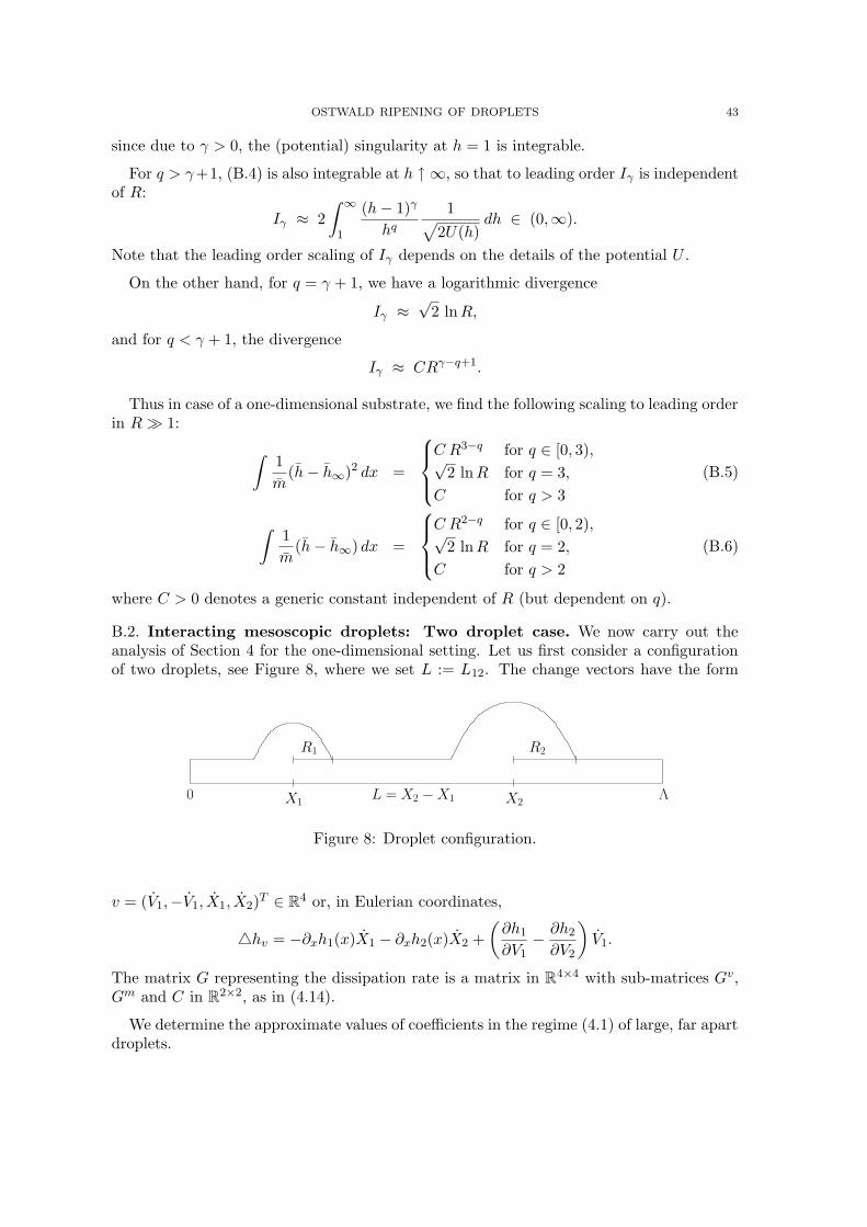
OSTWALD RIPENING OF DROPLETS 43
since due to γ > 0, the (potential) singularity at h = 1 is integrable.
For q > γ+1, (B.4) is also integrable at h ↑ ∞, so that to leading order Iγ is independentof R:
Iγ ≈ 2
∫ ∞
1
(h− 1)γ
hq1
√
2U(h)dh ∈ (0,∞).
Note that the leading order scaling of Iγ depends on the details of the potential U .
On the other hand, for q = γ + 1, we have a logarithmic divergence
Iγ ≈√
2 lnR,
and for q < γ + 1, the divergence
Iγ ≈ CRγ−q+1.
Thus in case of a one-dimensional substrate, we find the following scaling to leading orderin R� 1:
∫1
m(h− h∞)2 dx =
C R3−q for q ∈ [0, 3),√2 lnR for q = 3,
C for q > 3
(B.5)
∫1
m(h− h∞) dx =
C R2−q for q ∈ [0, 2),√2 lnR for q = 2,
C for q > 2
(B.6)
where C > 0 denotes a generic constant independent of R (but dependent on q).
B.2. Interacting mesoscopic droplets: Two droplet case. We now carry out theanalysis of Section 4 for the one-dimensional setting. Let us first consider a configurationof two droplets, see Figure 8, where we set L := L12. The change vectors have the form
X1 X2
R1 R2
L = X2 −X10 Λ
Figure 8: Droplet configuration.
v = (V1,−V1, X1, X2)T ∈ R
4 or, in Eulerian coordinates,
4hv = −∂xh1(x)X1 − ∂xh2(x)X2 +
(∂h1
∂V1− ∂h2
∂V2
)
V1.
The matrix G representing the dissipation rate is a matrix in R4×4 with sub-matrices Gv,
Gm and C in R2×2, as in (4.14).
We determine the approximate values of coefficients in the regime (4.1) of large, far apartdroplets.
44 KARL GLASNER, FELIX OTTO, TOBIAS RUMP AND DEJAN SLEPCEV
Computing Gv. Let w := (1,−1, 0, 0)T . Then −∂xJw = 4hw = ∂h1
∂V1− ∂h2
∂V2. Hence
wTGw = Gv11 −Gv12 −Gv21 +Gv22
=
∫1
m(h(x))|Jw(x)|2 dx
The above is the only requirement on coefficients of Gv, which allows us to define
Gv11 = Gv22 := 0
Gv12 = Gv21 := −12
∫1
m(h(x))|Jw|2 dx.
Elementary integration yields
Jw(x) =
0 outside,
− 16√
2ωV
− 3
2
1 (x−X1)3 − 1
4√
2ωV
− 1
2
1 (x−X1)− 12 in B(X1, R1),
−1 in between,
16√
2ωV
− 3
2
2 (x−X2)3 + 1
4√
2ωV
− 1
2
2 (x−X2)− 12 in B(X2, R2),
0 outside.
In the regime L� Ri, the dissipation tensor is to the leading order
∫1
m|Jw|2 dx =
∫
B(X1,R1)
1
m|Jw|2 dx+
∫ X2−R2
X1+R1
1 dx
︸ ︷︷ ︸
≈L
+
∫
B(X2,R2)
1
m|Jw|2 dx ≈ L,
since the two integrals over B(Xi, Ri) scale like Ri. In conclusion
Gvii = 0 (B.7a)
Gv12 = Gv21 ≈ −12L. (B.7b)
Computing Gm. Let w1 := (0, 0, 1, 0)T and w2 := (0, 0, 0, 1)T . Then −∂xJwi= 4hwi
=−∂xhi, for i = 1, 2. Hence
Gmii = wTi Gwi =
∫1
m(h(x))|Jwi
(x)|2 dx.
Elementary integration yields Jwi(x) = hi(x) and thus
Gmii =
∫1
m(h(x))(hi(x))
2 dx =: gi. (B.8a)
Since Jwihas support in B(Xi, Ri), it follows that
Gm12 = Gm21 =
∫1
m(h(x))Jw1
(x) · Jw2(x) dx = 0. (B.8b)
OSTWALD RIPENING OF DROPLETS 45
Computing C. For i = 1, 2
wTi Gw = Ci1 − Ci2
=
∫1
m(h(x))Jwi
(x) · Jw(x) dx, where−∂xJwi
= −∂xhi−∂xJw = ∂h1
∂V1− ∂h2
∂V2
=
∫
B(Xi,Ri)
1
m(h(x))hi(x)(c(x−Xi)
3 + c(x−Xi)− 12) dx
= −12
∫
B(Xi,Ri)
1
m(h(x))hi(x) dx.
This allows us to define
C11 = C22 = 0, (B.9a)
C12 = c1 := 12
∫
B(X1,R1)
1
m(h(x))h1(x) dx, (B.9b)
C21 = −c2 := −12
∫
B(X2,R2)
1
m(h(x))h2(x) dx. (B.9c)
Collecting the results of (B.8), (B.7) and (B.9), the full matrix G is given by
G =
0 −12L 0 −1
2
∫1mh2 dx
−12L 0 1
2
∫1mh1 dx 0
0 12
∫1mh1 dx
∫1mh
21 dx 0
−12
∫1mh2 dx 0 0
∫1mh
22 dx
(B.10)
to the leading order.
Rayleigh dynamics. Note that ∇E =√
2ω (V
− 1
2
1 , V− 1
2
2 , 0, 0)T . According to (4.13), coordi-
nates of Θ = (V1, V2, X1, X2)T are the solutions of the following system of linear ODEs:
V1 + V2 = 0,
Gv12(V2 − V1)− c2X2 − c1X1 = −√
2
ω(V
− 1
2
1 − V − 1
2
2 ),
c1V2 + g1X1 = 0,
−c2V1 + g2X2 = 0.
Solving the system yields for the volume change
V1 =
√2
ω
(c21g1
+c22g2
+ 2Gv12
)−1
(V− 1
2
1 − V − 1
2
2 ),
and for the migration
X1 =
√2
ω
c1g1
(c21g1
+c22g2
+ 2Gv12
)−1
(V− 1
2
1 − V − 1
2
2 ).
Note that in the regime L � V1
2
i , using the estimates on the coefficients from (B.5) and
(B.6) we obtain Gv12 �c21
g1+
c22
g2, so that
(c21g1
+c22g2
+ 2Gv12
)
≈ 2Gv12 ≈ −L.
46 KARL GLASNER, FELIX OTTO, TOBIAS RUMP AND DEJAN SLEPCEV
Therefore
V1 =
√2
ω
1
L(V
− 1
2
2 − V − 1
2
1 ), (B.11)
X1 =
√2
ω
1
L
∫1
m(h) h1dx∫
1m(h) h
21dx
(V− 1
2
2 − V − 1
2
1 ). (B.12)
B.3. Interacting mesoscopic droplets: n-droplet case. The computation of the ma-trix G in R
2n×2n is analogous to the two-droplet case. In particular,
Gvij = −12Lij ,
C = diag(c1, . . . , cn)T, where Tij :=
1 if i < j,0 if i = j,−1 if i > j,
Gm = diag(g1, . . . , gn).
(B.13)
It is easy to check that the choice Gvij = −1
2Lij is consistent with (B.7).
To determine the dynamics in a transparent form, assume that Xi < Xi+1 for all i =1, . . . , n − 1. Let us use the notation V = (V1, . . . , Vn)
T and X = (X1, . . . , Xn)T . The
equations of the dynamics are then
(I − ppT )(GvV + CT X) = −(I − ppT )∇VECV +GmX = 0.
Here, p has been restricted to its first n coordinates. It follows that
X = − diag
(c1g1, . . . ,
cngn
)
T V . (B.14)
Substituting in the first equation and observing that, as for two droplets,
C(Gm)−1CT � Gv
gives the following approximation when Lij � V1
2
k � 1 for i, j, k = 1, . . . , n, i 6= j:
(I − ppT )GvV = −(I − ppT )∇VE. (B.15)
The remainder of this subsection is devoted to finding a solution of this equation with∑
i V = 0. For this purpose, note that the submatrix Gv has the form of a Green’s function
in one dimension: The i-th entry of the product Gv V , i.e.
−12
∑
j 6=i|Xi −Xj | Vj ,
realizes the superposition of potentials inXi generated by “mass sources” atXj with masses
Vj . Thus, it is reasonable that equation (B.15) can be solved by applying a discrete Laplaceoperator D, that has the form of a tridiagonal matrix:
Dij :=
1Li−1 i
if j = i− 1
−(
1Li−1 i
+ 1Li i+1
)
if j = i1
Li i+1if j = i+ 1
0 else,
OSTWALD RIPENING OF DROPLETS 47
with no-flux condition at the boundary. We used the convention L0 1 = ∞ Lnn+1 = ∞.Note that D(I − ppT ) = D.
Indeed, a direct calculation of −DGv based on the relation Li j+1 = Li j + Lj j+1 yields
−DGv = 12
1 −1 . . . . . . −12
. . .
2−1 . . . . . . −1 1
,
and finally, using the conservation of volume∑
i Vi = 0, the identity
−DGvV = V .
Applying the same transformation to the right hand side gives for i = 1, . . . , n
(∇E)i+1 − (∇E)iLi i+1
− (∇E)i − (∇E)i−1
Li−1 i=
√2
ω
V
− 1
2
i+1 − V− 1
2
i
Li i+1− V
− 1
2
i − V − 1
2
i−1
Li−1 i
,
where we let L01 = Lnn+1 = ∞. Hence, we obtain the equation for the volume changegiven by (B.15):
Vi =
√2
ω
V
− 1
2
i+1 − V− 1
2
i
Li i+1− V
− 1
2
i − V − 1
2
i−1
Li−1 i
. (B.16)
To determine X, we use (B.14). It follows from (B.16) that
Xi =
√2
ω
∫1
m(h) hidx∫
1m(h) h
2i dx
V
− 1
2
i − V − 1
2
i−1
Li−1 i+V
− 1
2
i+1 − V− 1
2
i
Li i+1
. (B.17)
Now it is easy to check that equations (B.16) and (B.17) indeed coincide with the equa-tions of motion and pressure change proposed by Glasner and Witelski in [5]. To switch
between the volume and the pressure one applies the relation Pi =√
2ω V
− 1
2
i .
B.4. Time scales in the dynamics. From (B.11) and (B.12), we can deduce heuristicallythe typical time scale for Ostwald ripening and migration for a configuration of many
droplets. We recall the assumption L� V1
2 .
Ostwald ripening. From (B.11) we obtain
V ∼ 1
LV − 1
2 .
Hence the time scale for ripening is
τrip ∼V
V∼ LV 3
2 ∼ V 5
2 /H. (B.18)
Here we used mass conservation (4.27).
48 KARL GLASNER, FELIX OTTO, TOBIAS RUMP AND DEJAN SLEPCEV
Migration. Equation (B.12) implies the scaling
L ∼ |X| ∼ c
g
1
LV − 1
2
and therefore
τmig ∼L
L∼ g
cL2V − 1
2 ∼ g
cV
3
2 /H2.
Here, g and c denote the coefficients of the migration and the coupling matrix, resp., for atypical droplet. From (B.5) and (B.6) we deduce the scaling
c
g= 1
2
∫
B(X,R)1mh dx
∫
B(X,R)1m(h)2 dx
∼
V − 1
2 q ∈ [0, 2),
V − 1
2 lnV q = 2,
Vq−3
2 q ∈ (2, 3),
ln−1 V q = 3,
1 q > 3.
(B.19)
Hence the time scale for the droplet migration is
τmig ∼V
5
2
H2
V1
2 q ∈ [0, 2),
V1
2 ln−1 V q = 2,
V3−q2 q ∈ (2, 3),
lnV q = 3,
1 q > 3.
(B.20)
The relative importance of migration depending on V and H can be deduced from thequotient of the time scales:
τripτmig
∼ H
V − 1
2 q ∈ [0, 2),
V − 1
2 lnV q = 2,
Vq−3
2 q ∈ (2, 3),
ln−1 V q = 3,
1 q > 3.
Appendix C. Approximations
C.1. Approximating pressures relevant to Gm and C. To validate approximations ofSubsection 4.3.2 it suffices to consider v1 = (02, X, 02)
T with X 6= 0 and associated pressureϕv1 , the solution of
∇ · (m∇ϕv1) = −∇h1 · X.We introduce the following, intermediate, approximation of ϕv1 : Let l =
√R2L. Let
ξ ∈ C∞([0,∞), [0, 1]) be a cut-off function supported on [0, 2] and equal to 1 on [0, 1]. Letξl(x) := ξ(|x|/l). Then define
ϕv1 := (1− ξl(x−X2))ΨX1,V1
(x−X1) + ξl(x−X2)ΨX1,V1
(X2 −X1). (C.1)
Let us denote the error term by ϕe := ϕv1 − ϕv1 . Let A be the annulus B(X2, 2l)\B(X2, l).Note that −∇ · (m∇ϕe) = 0 on R
2\A, and that on A
−∇·(m∇ϕe) = −∆ξl(x−X2)(Ψ1,V1(x−X1)−Ψ1,V1
(X2−X1))−2∇ξl(x−X2)·∇Ψ1,V1(x−X1).
OSTWALD RIPENING OF DROPLETS 49
Therefore on A, the dipolar form (4.9) of Ψ1,V1implies the estimate
|∇ · (m∇ϕe)| .1
l2|X|max
x∈A|∇Ψ1,V1
(|x−X1|)| l +1
l|X|max
x∈A|∇Ψ1,V1
(|x−X1|)|.
Estimates (3.28) imply, via (3.29) that for |x| > R1
|Ψ1,V1(x)| . |X| 1
|x|Vγ1 β(V1). (C.2)
Here γ = max{3 − q, 1}/3, β(V ) = lnV if q = 2 and β ≡ 1 otherwise. Via (3.23) it thenfollows: For x > |R1|
|∇Ψ1,V1(x)| . |X| 1
|x|2Vγ1 β(V1). (C.3)
Using this estimate we obtain that on A
|∇ · (m∇ϕe)| .|X|lV γ
1 β(V1)1
L2.
Since m ≥ 1 the standard a-priori elliptic estimates imply that
‖ϕe‖2L2 . ‖∇(m∇ϕe)‖2L2 .|X|2l2 L4
V 2γ1 β2(V1) l
2 ≤ |X|2
L4V 2γ
1 β2(V1).
In conclusion, 2
‖ϕv1 − ϕv1‖L2 .|X|L2
V γ1 β(V1)� |X|V γ−2/3
1 β(V1). (C.4)
The error made in replacing ϕv1 by Ψ1,V1in (4.39) can now be estimated as follows. Note
that on the support of ∇hV1,0, Ψ1,V1is equal to ϕv1 . The Cauchy–Schwarz inequality and
estimate (C.4) yield∫
R2
(ϕv1(x)−Ψ1,V1(x−X1))(∇hV1,0(x) · Y )dx . ‖ϕv1 − ϕv1‖L2 |Y |V 1/3
1
. |X||Y |V γ−1/31 β(V1)
� |X||Y |g1.The last estimate uses the estimates on g1 as stated in (4.20) (originally stated in (3.27)).
We now justify the estimate used in (4.40). Using that ϕv1 is constant on B(X2, R2) andthe symmetry of hV2,0, the estimates (C.2), (C.3), and (C.4), and boundedness of |∇hV2,0|we obtain via the Cauchy-Schwarz inequality
∣∣∣∣∣
∫
B(X2,R2)ϕv1 ∇hV2,0 · Y dx
∣∣∣∣∣≤∣∣∣∣∣
∫
B(X2,R2)(ϕv1 − ϕv1)∇hV2,0 · Y dx
∣∣∣∣∣+ 0
. ‖ϕv1 − ϕv1‖L2
(∫
B(X2,R2)|∇hV2
· Y |2dx) 1
2
. |X||Y | 1
L2V γ
1 β(V1)V1/32
= |X||Y | o(√g1g2).
(C.5)
2Note that the estimate does not depend on either l or V2, which is what allows this construction to becarried out in the case of n droplets.
50 KARL GLASNER, FELIX OTTO, TOBIAS RUMP AND DEJAN SLEPCEV
We now validate the approximations used in computing the matrix C, in Subsection4.3.3. Using estimates (C.2),(C.3), and (C.4), the form of ∂h
∂V computed in (4.4), and theCauchy–Schwarz inequality we obtain:
∫
|ϕv1 − ϕv1 |(∣∣∣∣
∂h1
∂V1
∣∣∣∣+
∣∣∣∣
∂h2
∂V2
∣∣∣∣
)
. ‖ϕv1 − ϕv1‖L2
(∥∥∥∥
∂hV1,0
∂V1
∥∥∥∥L2
+
∥∥∥∥
∂hV2,0
∂V2
∥∥∥∥L2
)
.|X|L2
V γ1 β(V1)(V
−1/31 + V
−1/32 ) (C.6)
� |X|Ψ1,V1(|X2 −X1|).
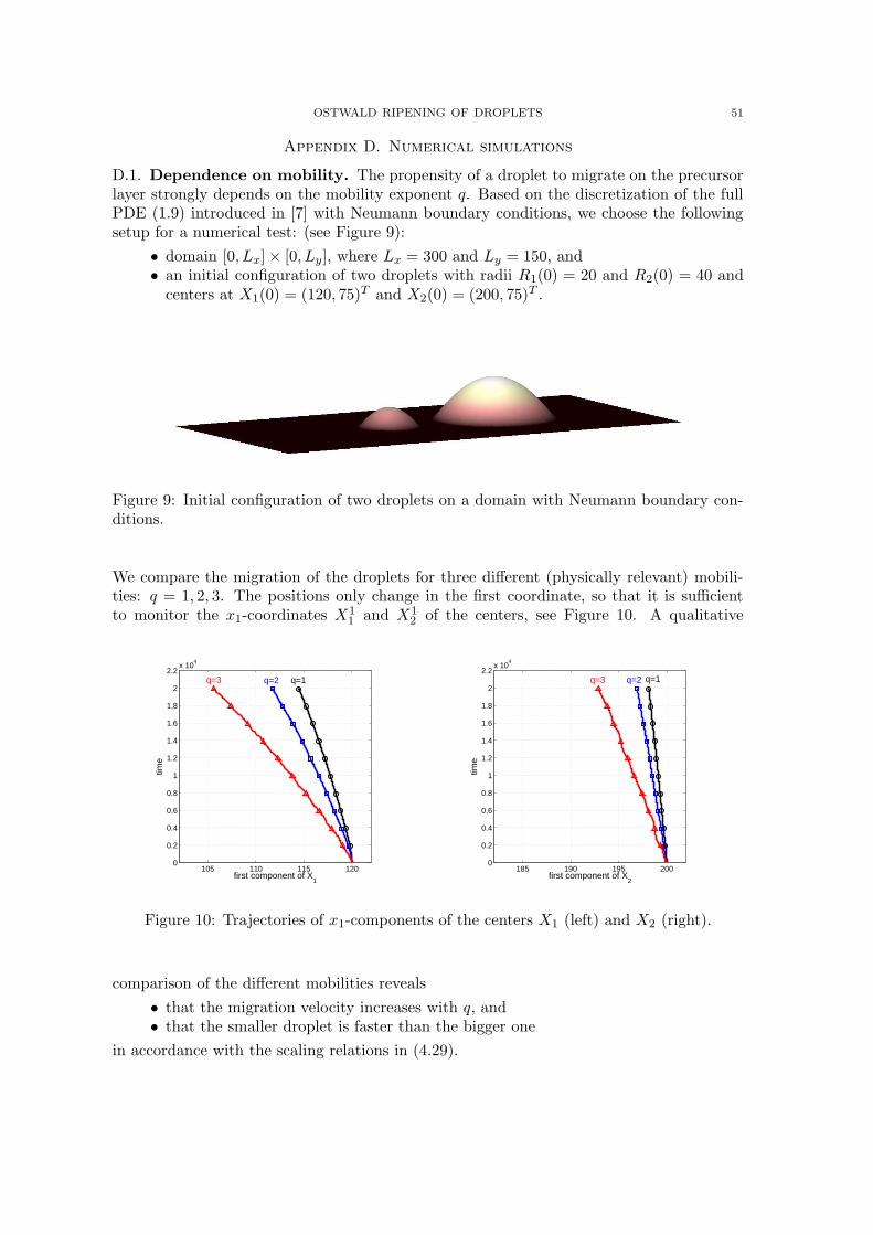
OSTWALD RIPENING OF DROPLETS 51
Appendix D. Numerical simulations
D.1. Dependence on mobility. The propensity of a droplet to migrate on the precursorlayer strongly depends on the mobility exponent q. Based on the discretization of the fullPDE (1.9) introduced in [7] with Neumann boundary conditions, we choose the followingsetup for a numerical test: (see Figure 9):
• domain [0, Lx]× [0, Ly], where Lx = 300 and Ly = 150, and• an initial configuration of two droplets with radii R1(0) = 20 and R2(0) = 40 and
centers at X1(0) = (120, 75)T and X2(0) = (200, 75)T .
Figure 9: Initial configuration of two droplets on a domain with Neumann boundary con-ditions.
We compare the migration of the droplets for three different (physically relevant) mobili-ties: q = 1, 2, 3. The positions only change in the first coordinate, so that it is sufficientto monitor the x1-coordinates X1
1 and X12 of the centers, see Figure 10. A qualitative
105 110 115 1200
0.2
0.4
0.6
0.8
1
1.2
1.4
1.6
1.8
2
2.2x 10
4
first component of X1
time
q=3 q=2 q=1
185 190 195 2000
0.2
0.4
0.6
0.8
1
1.2
1.4
1.6
1.8
2
2.2x 10
4
first component of X2
time
q=3 q=2 q=1
Figure 10: Trajectories of x1-components of the centers X1 (left) and X2 (right).
comparison of the different mobilities reveals
• that the migration velocity increases with q, and• that the smaller droplet is faster than the bigger one
in accordance with the scaling relations in (4.29).
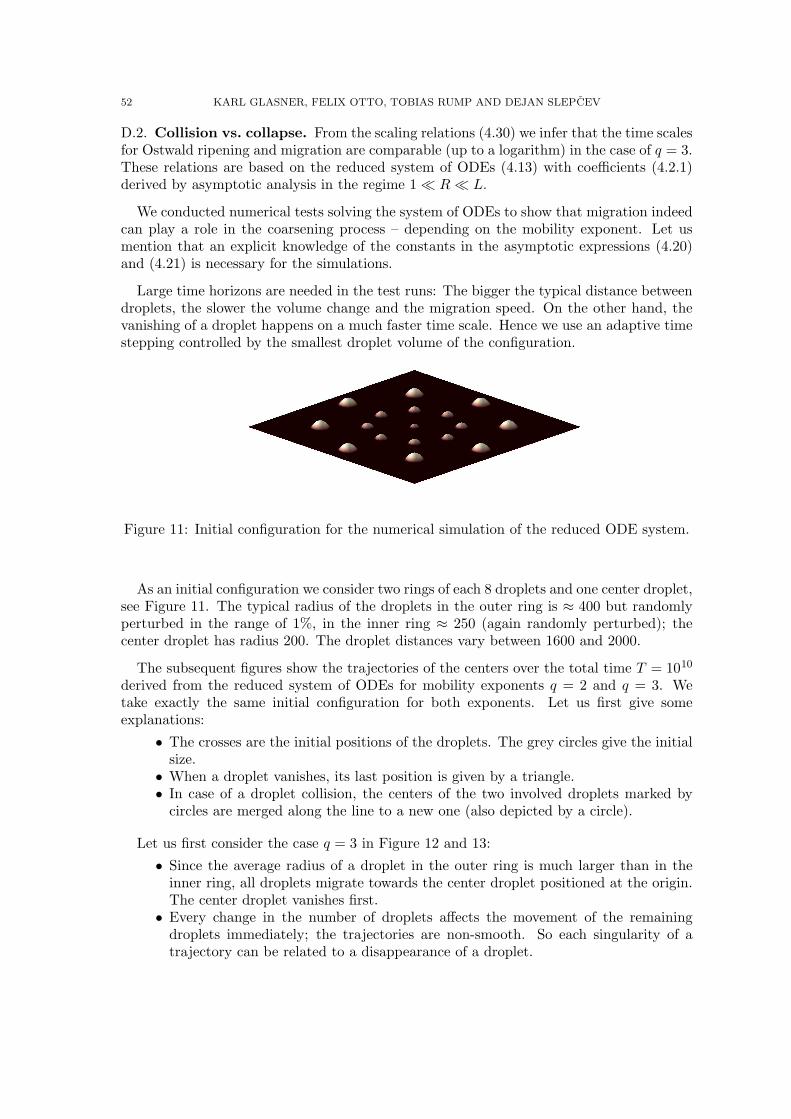
52 KARL GLASNER, FELIX OTTO, TOBIAS RUMP AND DEJAN SLEPCEV
D.2. Collision vs. collapse. From the scaling relations (4.30) we infer that the time scalesfor Ostwald ripening and migration are comparable (up to a logarithm) in the case of q = 3.These relations are based on the reduced system of ODEs (4.13) with coefficients (4.2.1)derived by asymptotic analysis in the regime 1� R� L.
We conducted numerical tests solving the system of ODEs to show that migration indeedcan play a role in the coarsening process – depending on the mobility exponent. Let usmention that an explicit knowledge of the constants in the asymptotic expressions (4.20)and (4.21) is necessary for the simulations.
Large time horizons are needed in the test runs: The bigger the typical distance betweendroplets, the slower the volume change and the migration speed. On the other hand, thevanishing of a droplet happens on a much faster time scale. Hence we use an adaptive timestepping controlled by the smallest droplet volume of the configuration.
Figure 11: Initial configuration for the numerical simulation of the reduced ODE system.
As an initial configuration we consider two rings of each 8 droplets and one center droplet,see Figure 11. The typical radius of the droplets in the outer ring is ≈ 400 but randomlyperturbed in the range of 1%, in the inner ring ≈ 250 (again randomly perturbed); thecenter droplet has radius 200. The droplet distances vary between 1600 and 2000.
The subsequent figures show the trajectories of the centers over the total time T = 1010
derived from the reduced system of ODEs for mobility exponents q = 2 and q = 3. Wetake exactly the same initial configuration for both exponents. Let us first give someexplanations:
• The crosses are the initial positions of the droplets. The grey circles give the initialsize.• When a droplet vanishes, its last position is given by a triangle.• In case of a droplet collision, the centers of the two involved droplets marked by
circles are merged along the line to a new one (also depicted by a circle).
Let us first consider the case q = 3 in Figure 12 and 13:
• Since the average radius of a droplet in the outer ring is much larger than in theinner ring, all droplets migrate towards the center droplet positioned at the origin.The center droplet vanishes first.• Every change in the number of droplets affects the movement of the remaining
droplets immediately; the trajectories are non-smooth. So each singularity of atrajectory can be related to a disappearance of a droplet.
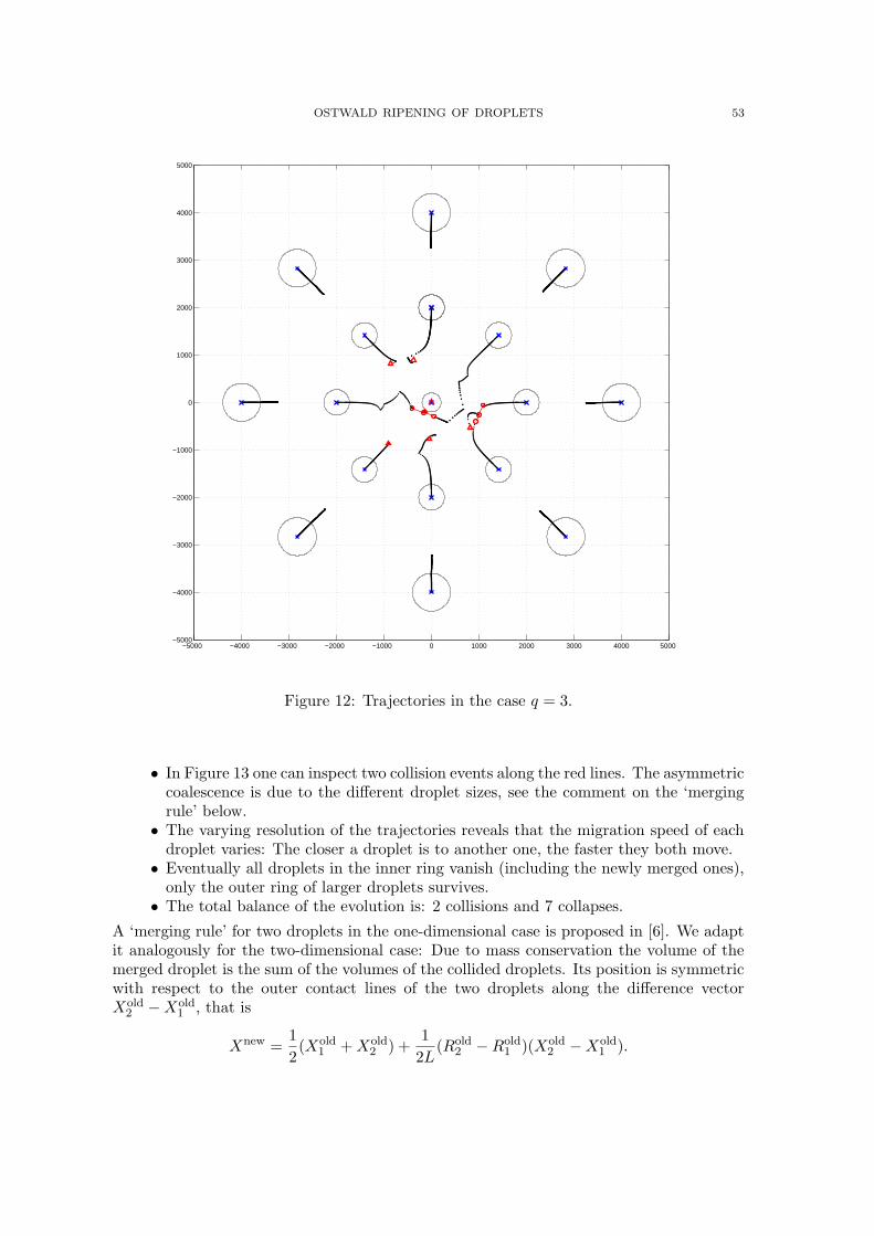
OSTWALD RIPENING OF DROPLETS 53
−5000 −4000 −3000 −2000 −1000 0 1000 2000 3000 4000 5000 −5000
−4000
−3000
−2000
−1000
0
1000
2000
3000
4000
5000
Figure 12: Trajectories in the case q = 3.
• In Figure 13 one can inspect two collision events along the red lines. The asymmetriccoalescence is due to the different droplet sizes, see the comment on the ‘mergingrule’ below.• The varying resolution of the trajectories reveals that the migration speed of each
droplet varies: The closer a droplet is to another one, the faster they both move.• Eventually all droplets in the inner ring vanish (including the newly merged ones),
only the outer ring of larger droplets survives.• The total balance of the evolution is: 2 collisions and 7 collapses.
A ‘merging rule’ for two droplets in the one-dimensional case is proposed in [6]. We adaptit analogously for the two-dimensional case: Due to mass conservation the volume of themerged droplet is the sum of the volumes of the collided droplets. Its position is symmetricwith respect to the outer contact lines of the two droplets along the difference vectorXold
2 −Xold1 , that is
Xnew =1
2(Xold
1 +Xold2 ) +
1
2L(Rold
2 −Rold1 )(Xold
2 −Xold1 ).
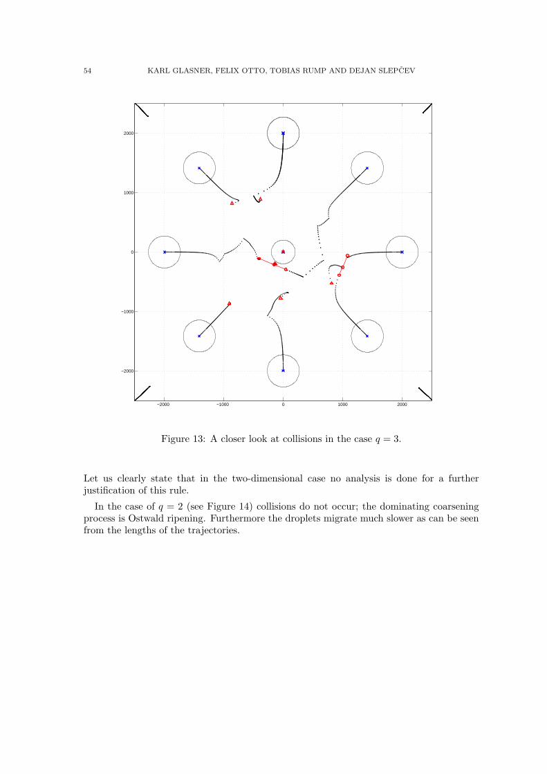
54 KARL GLASNER, FELIX OTTO, TOBIAS RUMP AND DEJAN SLEPCEV
−2000 −1000 0 1000 2000
−2000
−1000
0
1000
2000
Figure 13: A closer look at collisions in the case q = 3.
Let us clearly state that in the two-dimensional case no analysis is done for a furtherjustification of this rule.
In the case of q = 2 (see Figure 14) collisions do not occur; the dominating coarseningprocess is Ostwald ripening. Furthermore the droplets migrate much slower as can be seenfrom the lengths of the trajectories.
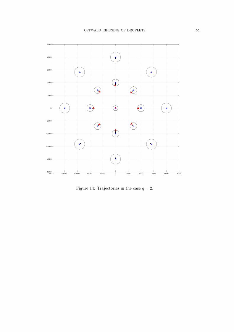
OSTWALD RIPENING OF DROPLETS 55
−5000 −4000 −3000 −2000 −1000 0 1000 2000 3000 4000 5000−5000
−4000
−3000
−2000
−1000
0
1000
2000
3000
4000
5000
Figure 14: Trajectories in the case q = 2.
56 KARL GLASNER, FELIX OTTO, TOBIAS RUMP AND DEJAN SLEPCEV
Appendix E. Relationship to matched asymptotic expansions
Much of the foregoing analysis can also be phrased in the language of matched asymptoticexpansions [4]. Here we briefly summarize the connections between the current presentationand this alternative approach.
The asymptotic droplet profiles (2.22-2.24) and other approximations were derived underthe assumption of large droplet height compared to a fixed precursor thickness. This iseffectively the same regime as rescaling all lengths so the droplets have size of order unityand the precursor film layer has thickness ε� 1. The width of the foot region under sucha rescaling is of order ε, which prompts the use of different asymptotic expansions in threeregions:
• Precursor region: The solution is expanded as h = εh1 + ε2h2 + . . .. The correc-tion term h2 satisfies the exterior Laplace equation that describes quasistationarydiffusion, whose boundary conditions are given by matching across the foot layersof each droplet. The flux which the droplets experience arises at this level in thesame fashion as flux arises in the Mullins-Sekerka reduction of the Cahn-Hilliardequation [8].• Foot region: The solution has the expansion h = εH1(z) + ε2H2(z) + . . . wherez = (R(t)−r)/ε is a stretched radial coordinate. The leading order solution recoversthe foot region solution given implicitly in equation (2.15).• Cap region: The solution has the expansion h = h0 + εαh1 + . . .. At leading order
one recovers the parabolic cap solution (2.22-2.24). The exponent α depends on qand is determined by matching requirements.
The expansions in the foot and cap region are carried to further orders whose scaling inε is prescribed by the mobility exponent q. These choices ultimately lead to matching con-ditions between the foot and cap layers, and a scaling relations for the dynamics. The casesq = 2, 3 are somewhat special because they lead to logarithmic terms in the expansions.
In the cap and foot regions, the correction terms (call them h′) satisfy a linear equationof the form
MLh′ = f, where Mµ = −∇ · (m∇µ) and Lh′ = −∆h′ + U ′′(h0)h′. (E.1)
Fredholm-type solvability conditions are derived from (null) eigenfunctions ψ of the adjointproblem, which can be written
Lh′0 = 0, Mψ = h′0. (E.2)
The relevant solution for migration is h′0 = ∂1h, from which we see that ψ solves the sameproblem as ψ1 in equation (3.17). The difference is that (3.17) is determined using thedetailed droplet profile rather than the leading order terms in the asymptotic expansions.The conclusion (3.19) is therefore a type of solvability condition as explained in section 3.1.Not surprisingly, the matched asymptotic analysis produces formulas for the migrationdynamics which have the same structure.
There is another solvability condition that gives the dynamics of the droplet radii interms of the flux transmitted across the foot region. This results in mass exchange be-tween droplets as in conventional Ostwald ripening. The net result of all this is to specifythe droplet dynamics in terms of flux which arises from quasistationary diffusion in theprecursor region.
Finally, the matched asymptotic approximation can be further reconnected to the re-duced gradient flow approximation of Section 4. This arises as follows. The exteriorLaplace equation (for quasistationary diffusion) satisfied in the precursor region can be
OSTWALD RIPENING OF DROPLETS 57
further approximated by use of Green’s functions. This approximation scheme turns out togive a reduced dynamical system essentially equivalent to the reduced gradient flow (e.g.(4.25-4.26)).
Acknowledgements. Felix Otto acknowledges partial support by the Sonderforschungs-bereich 611 Singular phenomena and scaling in mathematical models at Bonn University.Tobias Rump acknowledges support by the Sonderforschungsbereich 611. Dejan Slepcevwould like to thank University of Bonn for hospitality and acknowledge the support fromNSF through the grant DMS-0638481. Karl Glasner acknowledges support under NSFaward DMS-0405596, and thanks the University of Bonn for their hospitality.
References
[1] N. D. Alikakos and G. Fusco. Ostwald ripening for dilute systems under quasistationary dynamics.Comm. Math. Phys., 238(3):429–479, 2003.
[2] N. D. Alikakos, G. Fusco, and G. Karali. The effect of the geometry of the particle distribution inOstwald ripening. Comm. Math. Phys., 238(3):481–488, 2003.
[3] C. M. Elliott and H. Garcke. On the Cahn-Hilliard equation with degenerate mobility. SIAM J. Math.
Anal., 27(2):404–423, 1996.[4] K. B. Glasner. Ostwald ripening in thin film equations. in preparation, 2007.[5] K. B. Glasner and T. P. Witelski. Coarsening dynamics of dewetting films. Phys. Rev. E, 67(1):016302,
2003.[6] K. B. Glasner and T. P. Witelski. Collision versus collapse of droplets in coarsening of dewetting thin
films. Phys. D, 209(1-4):80–104, 2005.[7] F. Otto, T. Rump, and D. Slepcev. Coarsening rates for a droplet model: Rigorous upper bounds. SIAM
J. Math. Anal., 38(2):503–529 (electronic), 2006.[8] R. L. Pego. Front migration in the nonlinear Cahn-Hilliard equation. Proc. Roy. Soc. London Ser. A,
422(1863):261–278, 1989.[9] L. M. Pismen and Y. Pomeau. Mobility and interactions of weakly nonwetting droplets. Phys. Fluids,
16(7):2604–2612, 2004.
Karl Glasner, Department of Mathematics, University of Arizona, 617 N. Santa Rita,
Tucson, AZ 85721, U.S.A.
E-mail address: [email protected]
Felix Otto, Institute for Applied Mathematics, University of Bonn, Wegelerstraße 10,
D–53115 Bonn, Germany
E-mail address: [email protected]
Tobias Rump, Institute for Applied Mathematics, University of Bonn, Wegelerstraße 10,
D–53115 Bonn, Germany
E-mail address: [email protected]
Dejan Slepcev, Department of Mathematical Sciences, Carnegie Mellon University, Pitts-
burgh, PA 15213, U.S.A.
E-mail address: [email protected]
Bestellungen nimmt entgegen: Institut für Angewandte Mathematik der Universität Bonn Sonderforschungsbereich 611 Wegelerstr. 6 D - 53115 Bonn Telefon: 0228/73 4882 Telefax: 0228/73 7864 E-mail: [email protected] http://www.iam.uni-bonn.de/sfb611/
Verzeichnis der erschienenen Preprints ab No. 310
310. Eberle, Andreas; Marinelli, Carlo: Stability of Sequential Markov Chain Monte Carlo Methods 311. Eberle, Andreas; Marinelli, Carlo: Convergence of Sequential Markov Chain Monte Carlo Methods: I. Nonlinear Flow of Probability Measures 312. Albeverio, Sergio; Hryniv, Rostyslav; Mykytyuk, Yaroslav: Reconstruction of Radial Dirac and Schrödinger Operators from Two Spectra 313. Eppler, Karsten; Harbrecht, Helmut: Tracking Neumann Data for Stationary Free Boundary Problems 314. Albeverio, Sergio; Mandrekar, Vidyadhar; Rüdiger, Barbara: Existence of Mild Solutions for Stochastic Differential Equations and Semilinear Equations with Non-Gaussian Lévy Noise 315. Albeverio, Sergio; Baranovskyi, Oleksandr; Pratsiovytyi, Mykola; Torbin, Grygoriy: The Set of Incomplete Sums of the First Ostrogradsky Series and Anomalously Fractal Probability Distributions on it 316. Gottschalk, Hanno; Smii, Boubaker: How to Determine the Law of the Noise Driving a SPDE 317. Gottschalk, Hanno; Thaler, Horst: AdS/CFT Correspondence in the Euclidean Context 318. Gottschalk, Hanno; Hack, Thomas: On a Third S-Matrix in the Theory of Quantized Fields on Curved Spacetimes 319. Müller, Werner; Salomonsen, Gorm: Scattering Theory for the Laplacian on Manifolds with Bounded Curvature 320. Ignat, Radu; Otto, Felix: 2-d Compactness of the Néel Wall 321. Harbrecht, Helmut: A Newton Method for Bernoulli’s Free Boundary Problem in Three Dimensions 322. Albeverio, Sergio; Mitoma, Itaru: Asymptotic Expansion of Perturbative Chern-Simons Theory via Wiener Space 323. Marinelli, Carlo: Well-Posedness and Invariant Measures for HJM Models with Deterministic Volatility and Lévy Noise
324. Albeverio, Sergio; Ayupov, Sh. A.; Kudaybergenov, K. K.: Derivations on the Algebra of τ-Compact Operators Affiliated with a Type I von Neumann Algebra 325. Castaño Díez, Daniel; Gunzburger, Max; Kunoth, Angela: An Adaptive Wavelet Viscosity Method for Hyperbolic Conservation Laws 326. Albeverio, Sergio; Ayupov, Sh. A.; Omirov, B. A.; Khudoyberdiyev, A. Kh: n-Dimensional Filiform Leibniz Algebras of Length (n-1) and Their Derivations 327. Albeverio, Sergio; Rabanovich, Slavik: On a Class of Unitary Representations of the Braid Groups B3 and B4
328. Husseini, Ryad; Kassmann, Moritz: Markov Chain Approximations for Symmetric Jump Processes 329. Marinelli, Carlo: Local Well-Posedness of Musiela's SPDE with Lévy Noise 330. Frehse, Jens; Steinhauer, Mark; Weigant, Wladimir: On Stationary Solutions for 2 - D Viscous Compressible Isothermal Navier-Stokes Equations; erscheint in: Journal of Mathematical Fluid Mechanics 331. Müller, Werner: A Spectral Interpretation of the Zeros of the Constant Term of Certain Eisenstein Series 332. Albeverio, Sergio; Mazzucchi, Sonia: The Trace Formula for the Heat Semigroup with Polynomial Potential 333. Málek, Josef; Pražák, Dalibor; Steinhauer, Mark: On the Existence and Regularity of Solutions for Degenerate Power-Law Fluids; erscheint in: Differential and Integral Equations 334. Gwiazda, Piotr; Málek, Josef; Świerczewska, Agnieszka: On Flows of an Incompressible Fluid with Discontinuous Power-Law-Like Rheology; erscheint in: Control, Optimization and Calculus of Variations 335. Diening, Lars; Málek, Josef; Steinhauer, Mark: On Lipschitz Truncations of Sobolev Functions (with Variable Exponent) and Their Selected Applications; erscheint in: Control, Optimization and Calculus of Variations 336. Frehse, Jens; Weigant, Wladimir: On Quasi-Stationary Models of Mixtures of Compressible Fluids 337. Frehse, Jens; Steinhauer, Mark; Weigant, Wladimir: The Dirichlet Problem for Viscous Compressible Isothermal Navier-Stokes Equations in Two-Dimensions 338. Capella, Antonio; Melcher, Christof; Otto, Felix: Wave-Type Dynamics in Ferromagnetic Thin Film and the Motion of Néel Walls 339. Glasner, Karl; Otto, Felix; Rump, Tobias; Slepčev, Dejan: Ostwald Ripening of Droplets: The Role of Migration


![Single Molecule Microscopy and Hole-Burning Spectroscopy ...€¦ · droplets [xvi,xvii] using confocal microscopes and sensitive optical detection schemes. Direct imaging of single](https://static.fdocument.pub/doc/165x107/5ed9264f6714ca7f47693d21/single-molecule-microscopy-and-hole-burning-spectroscopy-droplets-xvixvii.jpg)


