Operation of Holographic Elements with Broadband Light

Sources

Thesis by

Hung-Te Hsieh

In Partial Fulfillment of the Requirements

for the Degree of

Doctor of Philosophy

California Institute of Technology

Pasadena, California

2005

(Defended February 11, 2005)

ii

Material in chaper 4 is reprinted with permission from H. T. Hsieh, G. Panotopoulos, M. Liger,

Y. C. Tai and D. Psaltis, “Athermal holographic filters.” IEEE publication: Photonics Technology

Letters, 16(1), January 2004, pp. 177-179 c©2004 IEEE.

c© 2005

Hung-Te Hsieh

All Rights Reserved

iii

Acknowledgements

I would like to start by expressing tremendous gratitude for Professor Demetri Psaltis, my academic

advisor during the five years I spent at Caltech. His unwavering enthusiasm for science and the

remarkable professionalism he demonstrated deeply inspired me. I am greatly indebted to the

wonderful chance he granted me to come to Caltech and work on exciting projects with several

extraordinarily brilliant students. I would also like to thank Professor Karsten Buse dearly. I

enjoyed working productively in his marvelous laboratories. I was also impressed by his fruitful

devotion not only to science but also to his group as a caring big brother. The eight months I spent

in his group at the University of Bonn are very special in my life. Wonderful memories abound:

hiking through the snowy Goethe’s trail in Brocken, strolling around in the Christmas market in

wide-eyed curiosity, cycling along the Rhein river... etc.

One precious privilege of studying at Caltech is the pleasure of getting to know some of the

brightest souls in the world. I am glad I have the chance to show my appreciation here. Wenhai Liu,

who took me to my first dinner in America. Greg Steckman, Chris Moser, Greg Bollock. Zhiwen

Liu, my intellectual idol, who warmly shared his brilliant physical insights and made them feel like

a breeze! George Panotopoulos, my best mentor, who taught me almost everything I know working

in an optics lab and then a lot more about life. I had the best time working with him on the

holographic filter project. Jose Mumbru, my Star Wars hero, who is blessed with such a sense of

humor you need to invent a new word for humorous. The tapas in Barcelona and paella in Alicante

I had with him are among the most enjoyable meals I remember. Yunping Yang, who was always

generous with his valuable advice. Irena Maravic, for some most enlightening conversations. Martın

and his most lovely wife Lucıa, who offer me the warmest friendship and the fantastic chance to

experience first-hand the way Spaniards wed and party! Emmanouil-Panagiotis Fitrakis, thanks to

whom my strenuous first year and the following intensive lab work did not turn my life anemic in

fun. Todd Meyrath; Zhenyu Li, whose kind heart and sense of responsibility will definitely get him

far. Hua Long, George Maltezos, Vijay Gupta and Dirk Walther. Dr. Ye Pu, for his help with my

femtosecond experiments. Dr. David Erickson, who impressed me with his dedication to work. I

also admire the tenacity and exceptional capability of the “new generation”: James Adleman, Eric

Ostby, Troy Rockwood and Mankei Tsang. And Baiyang Li, for the eye-opening and life-changing

iv

conversations on cross-strait relationship.

I want to thank Yayun Liu for meeting some of my most uncanny needs in experiments and the

gift of useful advice to a 24-year-old who was going through culture shock. Lucinda Acosta, for her

competence in administrative affairs and most importantly, the passion we share for some of the most

life-enriching music and of course, Julienne. Linda Dozsa, for hailing me as a great photographer

and the best Champagne I ever drank! Teresita Legaspi, for her kind help in the Registrar’s Office.

My special thanks also go to Divina Bautista and Alice Sogomonian in the Health Center, who took

the best care of me after my horrible car accident.

Across the Atlantic Ocean, I have to deliver my most sincere appreciation to all the members

of Dr. Buse’s group for their soothing friendship during my sojourn. Especially to Oliver Beyer,

for the excellent collaboration we had in the femtosecond holography project and for welcoming

me into his great family in Osnabruck. Dr. Konrad Peithmann, who remains my favorite office

mate. Clemens von Korff Schmising and Dominik Maxein, for their indispensable help in the lab

and some crash courses in German. Dr. Boris Sturman, for his mathematical genius and valuable

suggestions. Ms. Raja Bernard, for preventing me from becoming an illegal immigrant in Germany.

Mark Wengler, Ulrich Hartwig and Helge Eggert, who took me out to a live jazz bar for a most

memorable adventure. Ingo Breunig, for the enjoyable barbecue party. Michael Kosters, for helping

me with the apartment and the successful collaboration. Drs. Elisabeth Soergel and Akos Hoffmann,

for the delicious Mexican-style dinner and a fun-filled night. Last but not least, I send my special

thanks to Ms. Elli Luhmer, my landlord, whose motherly care kept me warm at heart even on those

snowy days in Bonn.

My days as a graduate student would have been so lonely without my dearest friends, both in

Taiwan and America. Special thanks go to William Chang and Bartz Huang, who have always been

there for me through the years. Eric Cheng, with whom I enjoy exchanging banter. And of course

all the TGSA members at Caltech. Todd, who rescued me from the wrecked car. I would also like

to thank Russ for the incredible tolerance of my worst side and for being a constant in my life.

Finally, I would like to dedicate my thesis to my family, especially to my parents, whose immea-

surable and unconditional love and support make me want to be a more generous and better person.

Words cannot describe how much I love them.

v

Abstract

This thesis presents the theoretical and experimental investigation of volume holography operated

with broadband/polychromatic light sources, i.e., in both continuous-wave (linear) and femtosecond-

pulse (nonlinear) regimes.

The first chapter reviews the concept of volume holography and provides a tacit introduction to

some basic properties of volume holograms and compares the operation of holograms in the spatial

and temporal domains, preparing the readers for later chapters.

The second chapter introduces a powerful theoretical tool for the analysis of volume holograms

in the reflection geometry: the matrix formulation, laying the foundation for the application of

holographic gratings utilized as WDM filters.

The third chapter takes into consideration the effects of the practically inevitable finite beam-

widths. By means of Fourier decomposition, the deviation of the filtering properties of volume

holographic gratings from the ideal plane-wave case can be satisfactorily explained and predicted.

Experiments and simulations are performed and compared to confirm the validity of the theory.

Volume holographic gratings in the reflection geometry serve as excellent WDM filters for telecom-

munication purposes thanks to their low cross-talk and readily engineered filtering properties. The

theoretical design and experimental realization of athermal holographic filters are presented in the

fourth chapter. By incorporating a passive, thermally actuated MEMS mirror, the temperature

dependence of the Bragg wavelength of a holographic filter can be compensated.

The analysis of holographic gratings in the 90 degree geometry requires a two dimensional theory.

The relevant boundary conditions give rise to some peculiar behaviors in this configuration. Theory,

simulations and some experimental results of the 90-degree holography are presented in chapter five.

The sixth chapter delves into the subject of instantaneous Kerr index grating established by

two intense, interfering femtosecond (pump) pulses at 388 nm owing to the omnipresent third-order

nonlinearity. The coupled-mode equations describing the incident and diffracted (probe) pulses at

776 nm are written down; the solution is experimentally corroborated. It is further demonstrated

that the temporal resolution in such a holographic pump-probe configuration does not degrade

appreciably as the angular separation between pump pulses increases.

Chapter seven investigates the nonlinear absorption processes in lithium niobate crystals with

vi

femtosecond pulses. The model of two-photon absorption well explains and anticipates the transmis-

sion coefficients of single pulses over a wide range of intensity. Collinear pump-probe transmission

experiments are then carried out to look into the nonlinear absorption suffered by the probe pulse

at 776 nm owing to the pump pulse at 388 nm; the dependence of the probe pulse transmission

coefficient on the time delay between pump and probe pulses is characterized by a dip and a long-

lasting plateau, which are attributed, respectively, to direct two-photon transitions involving pump

and probe photons and the existence of free carriers.

Building on the experimental experience and theoretical understanding of the previous two chap-

ters, the results of holographic pump-probe experiments in lithium niobate crystals are presented in

the final chapter. The behavior is much more complicated because it encompasses all phenomena

explored in the two preceding chapters, i.e., both the real and imaginary parts of the third-order

susceptibility come into play in the instantaneous material response; furthermore, another mixed

grating due to excited charge carriers exists long after the pump pulses pass through. Valuable

information on the grating formation process is obtained thanks to the sub-picosecond temporal

resolution of such configurations.

vii

Contents

Acknowledgements iii

Abstract v

1 Introduction 1

1.1 Volume holographic gratings and their filtering properties . . . . . . . . . . . . . . . 1

1.2 Spatial-domain perspective . . . . . . . . . . . . . . . . . . . . . . . . . . . . . . . . 2

1.3 Temporal-domain perspective . . . . . . . . . . . . . . . . . . . . . . . . . . . . . . . 3

1.4 Recording and readout of holographic gratings with polychromatic light sources . . . 4

Bibliography 6

2 Matrix formulation for holographic filters in the reflection geometry 7

2.1 Matrix formulation for optical layered media . . . . . . . . . . . . . . . . . . . . . . 7

2.1.1 TE case . . . . . . . . . . . . . . . . . . . . . . . . . . . . . . . . . . . . . . . 8

2.1.2 TM case . . . . . . . . . . . . . . . . . . . . . . . . . . . . . . . . . . . . . . . 10

2.1.3 Diffraction efficiency of a multilayer medium . . . . . . . . . . . . . . . . . . 11

2.2 Matrix formulation for sinusoidal gratings . . . . . . . . . . . . . . . . . . . . . . . . 11

2.3 Experimental results . . . . . . . . . . . . . . . . . . . . . . . . . . . . . . . . . . . . 15

2.3.1 Recording holographic WDM filters in reflection geometry in LiNbO3 . . . . 15

2.3.2 Measured filter response . . . . . . . . . . . . . . . . . . . . . . . . . . . . . . 16

Bibliography 18

3 Beam-width dependent filtering properties of volume holographic gratings 19

3.1 Introduction . . . . . . . . . . . . . . . . . . . . . . . . . . . . . . . . . . . . . . . . . 19

3.2 Theoretical consideration . . . . . . . . . . . . . . . . . . . . . . . . . . . . . . . . . 20

3.3 Numerical simulations and experimental results . . . . . . . . . . . . . . . . . . . . . 22

3.3.1 Reflection geometry . . . . . . . . . . . . . . . . . . . . . . . . . . . . . . . . 22

3.3.1.1 Experimental setup . . . . . . . . . . . . . . . . . . . . . . . . . . . 23

viii

3.3.1.2 Wavelength selectivity . . . . . . . . . . . . . . . . . . . . . . . . . . 23

3.3.1.3 Angular selectivity . . . . . . . . . . . . . . . . . . . . . . . . . . . . 24

3.3.1.4 Diffracted beam profiles . . . . . . . . . . . . . . . . . . . . . . . . . 27

3.3.2 Transmission geometry . . . . . . . . . . . . . . . . . . . . . . . . . . . . . . . 27

3.3.2.1 Experimental setup . . . . . . . . . . . . . . . . . . . . . . . . . . . 27

3.3.2.2 Wavelength selectivity . . . . . . . . . . . . . . . . . . . . . . . . . . 28

3.3.2.3 Angular selectivity . . . . . . . . . . . . . . . . . . . . . . . . . . . . 28

3.3.2.4 Diffracted beam profiles . . . . . . . . . . . . . . . . . . . . . . . . . 29

3.4 Conclusion . . . . . . . . . . . . . . . . . . . . . . . . . . . . . . . . . . . . . . . . . 29

Bibliography 31

4 Athermal holographic filters 32

4.1 Introduction . . . . . . . . . . . . . . . . . . . . . . . . . . . . . . . . . . . . . . . . . 32

4.2 Theory . . . . . . . . . . . . . . . . . . . . . . . . . . . . . . . . . . . . . . . . . . . . 32

4.3 Experiment and results . . . . . . . . . . . . . . . . . . . . . . . . . . . . . . . . . . 34

4.4 Conclusions . . . . . . . . . . . . . . . . . . . . . . . . . . . . . . . . . . . . . . . . . 38

Bibliography 39

5 Holographic filters in the 90 degree geometry 40

5.1 Introduction . . . . . . . . . . . . . . . . . . . . . . . . . . . . . . . . . . . . . . . . . 40

5.2 Beam propagation in the 90 degree geometry holograms . . . . . . . . . . . . . . . . 41

5.3 Wavelength selectivity . . . . . . . . . . . . . . . . . . . . . . . . . . . . . . . . . . . 43

5.4 Numerical simulations . . . . . . . . . . . . . . . . . . . . . . . . . . . . . . . . . . . 44

5.5 Experimental results . . . . . . . . . . . . . . . . . . . . . . . . . . . . . . . . . . . . 48

5.5.1 Beam profile experiment . . . . . . . . . . . . . . . . . . . . . . . . . . . . . . 48

5.5.2 Filtering properties of the 90 degree geometry holograms . . . . . . . . . . . 53

5.6 Conclusion . . . . . . . . . . . . . . . . . . . . . . . . . . . . . . . . . . . . . . . . . 55

Bibliography 56

6 Femtosecond holography in Kerr media 57

6.1 Introduction . . . . . . . . . . . . . . . . . . . . . . . . . . . . . . . . . . . . . . . . . 57

6.2 Theory . . . . . . . . . . . . . . . . . . . . . . . . . . . . . . . . . . . . . . . . . . . . 59

6.2.1 Coupled mode equations for pulse holography . . . . . . . . . . . . . . . . . . 60

6.2.2 Solution of the diffracted pulse: undepleted incident probe . . . . . . . . . . . 62

6.3 Experimental results and discussion . . . . . . . . . . . . . . . . . . . . . . . . . . . 64

6.4 Conclusion . . . . . . . . . . . . . . . . . . . . . . . . . . . . . . . . . . . . . . . . . 68

ix

Bibliography 69

7 Nonlinear absorption processes in lithium niobate crystals investigated with fem-

tosecond light pulses 71

7.1 Introduction . . . . . . . . . . . . . . . . . . . . . . . . . . . . . . . . . . . . . . . . . 71

7.2 Collinear pump-and-probe experimental setup . . . . . . . . . . . . . . . . . . . . . . 72

7.3 Two-photon absorption process for a single femtosecond pulse . . . . . . . . . . . . . 74

7.3.1 Motivation . . . . . . . . . . . . . . . . . . . . . . . . . . . . . . . . . . . . . 74

7.3.2 Theory of two-photon absorption . . . . . . . . . . . . . . . . . . . . . . . . . 75

7.3.3 Experimental results . . . . . . . . . . . . . . . . . . . . . . . . . . . . . . . . 76

7.4 Collinear pump-and-probe experiment and modeling . . . . . . . . . . . . . . . . . . 79

7.4.1 Experimental results . . . . . . . . . . . . . . . . . . . . . . . . . . . . . . . . 79

7.4.2 Modeling of collinear pump-and-probe experiment . . . . . . . . . . . . . . . 80

7.4.2.1 Modeling the dip of Tr(∆t) . . . . . . . . . . . . . . . . . . . . . . . 80

7.4.2.2 Modeling the plateau of Tr(∆t) . . . . . . . . . . . . . . . . . . . . 81

7.4.3 Comparison between theory and experiments: the determination of parameters

βr and σr . . . . . . . . . . . . . . . . . . . . . . . . . . . . . . . . . . . . . . 84

7.5 Conclusion . . . . . . . . . . . . . . . . . . . . . . . . . . . . . . . . . . . . . . . . . 84

Bibliography 85

8 Femtosecond recording of spatial gratings and time-resolved readout in lithium

niobate 87

8.1 Introduction . . . . . . . . . . . . . . . . . . . . . . . . . . . . . . . . . . . . . . . . . 87

8.2 Experimental observation . . . . . . . . . . . . . . . . . . . . . . . . . . . . . . . . . 89

8.2.1 Experimental setup . . . . . . . . . . . . . . . . . . . . . . . . . . . . . . . . . 89

8.2.2 Polarization dependence . . . . . . . . . . . . . . . . . . . . . . . . . . . . . . 91

8.2.3 Dependence on dopants . . . . . . . . . . . . . . . . . . . . . . . . . . . . . . 93

8.3 Theoretical justification and comparison with experimental data . . . . . . . . . . . 94

8.3.1 Decoupling of pump pulses when qp = 2βpIp0d ≤ 1 . . . . . . . . . . . . . . . 95

8.3.2 Curve-fitting and the extracted Kerr coefficient of LiNbO3 . . . . . . . . . . . 96

8.3.3 Mixed grating due to the excited carriers . . . . . . . . . . . . . . . . . . . . 98

8.3.4 Intensity dependence of ηpeak and ηpl. . . . . . . . . . . . . . . . . . . . . . . 99

8.4 Conclusion . . . . . . . . . . . . . . . . . . . . . . . . . . . . . . . . . . . . . . . . . 100

Bibliography 101

x

List of Figures

1.1 A schematic illustration of the Bragg condition: the wavevectors of the optical fields

and the grating vector K constitute the sides of a triangle. . . . . . . . . . . . . . . . 1

1.2 Angular selectivity of a volume hologram. . . . . . . . . . . . . . . . . . . . . . . . . . 2

1.3 Wavelength selectivity of a volume hologram. . . . . . . . . . . . . . . . . . . . . . . . 3

1.4 Schematic illustrations of the recording and readout of holograms with monochromatic

and polychromatic light sources. . . . . . . . . . . . . . . . . . . . . . . . . . . . . . . 4

2.1 A sinusoidal grating structure. . . . . . . . . . . . . . . . . . . . . . . . . . . . . . . . 7

2.2 A stratified dielectric structure. The layers are homogeneous in the x and y dimensions.

The layer i has a thickness hi with a refractive index ni, where i = F, 1, 2 · · ·N, L. . . 8

2.3 The “slicing” of a single period of a sinusoidal grating structure. . . . . . . . . . . . . 12

2.4 Convergence of the effective matrix C of a single grating period Λ. . . . . . . . . . . . 12

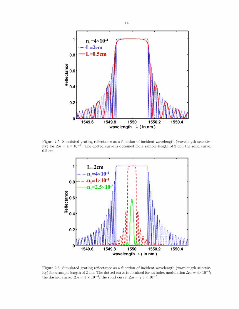
2.5 Simulated grating reflectance as a function of incident wavelength (wavelength selec-

tivity) for ∆n = 4 × 10−4. The dotted curve is obtained for a sample length of 2 cm;

the solid curve, 0.5 cm. . . . . . . . . . . . . . . . . . . . . . . . . . . . . . . . . . . . 14

2.6 Simulated grating reflectance as a function of incident wavelength (wavelength selectiv-

ity) for a sample length of 2 cm. The dotted curve is obtained for an index modulation

∆n = 4 × 10−4; the dashed curve, ∆n = 1 × 10−4; the solid curve, ∆n = 2.5 × 10−5. . 14

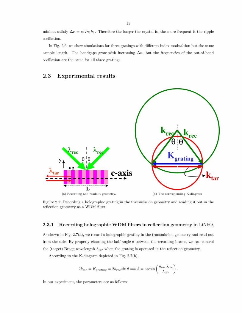
2.7 Recording a holographic grating in the transmission geometry and reading it out in the

reflection geometry as a WDM filter. . . . . . . . . . . . . . . . . . . . . . . . . . . . . 15

2.8 A recording curve of the holographic grating. (A stabilization system is incorporated

into the recording setup for optimal stability.) . . . . . . . . . . . . . . . . . . . . . . 16

2.9 Measured filter transmittance in the through channel. . . . . . . . . . . . . . . . . . . 17

3.1 Theoretical configuration. The volume holographic grating has a transfer function

H(ki;kd). VHGR/T is a volume holographic grating in the reflection/transmission

geometry. . . . . . . . . . . . . . . . . . . . . . . . . . . . . . . . . . . . . . . . . . . . 20

xi

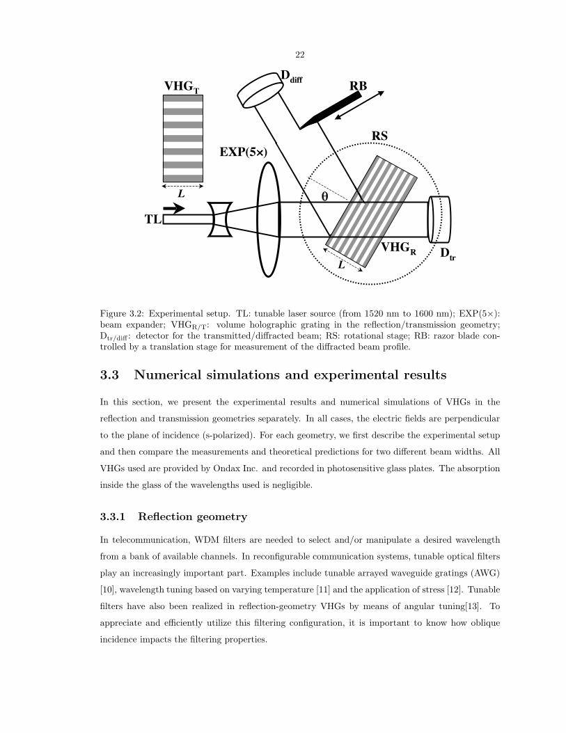
3.2 Experimental setup. TL: tunable laser source (from 1520 nm to 1600 nm); EXP(5×):

beam expander; VHGR/T: volume holographic grating in the reflection/transmission

geometry; Dtr/diff : detector for the transmitted/diffracted beam; RS: rotational stage;

RB: razor blade controlled by a translation stage for measurement of the diffracted

beam profile. . . . . . . . . . . . . . . . . . . . . . . . . . . . . . . . . . . . . . . . . . 22

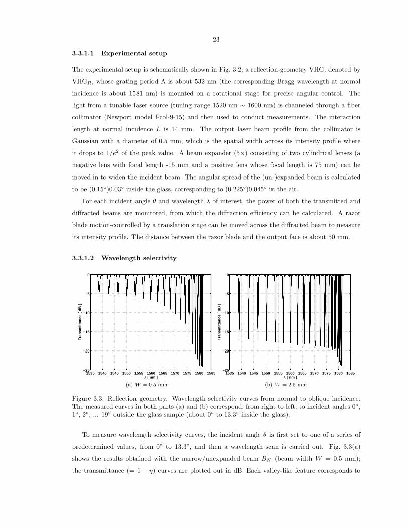
3.3 Reflection geometry. Wavelength selectivity curves from normal to oblique incidence.

The measured curves in both parts (a) and (b) correspond, from right to left, to incident

angles 0◦, 1◦, 2◦, ... 19◦ outside the glass sample (about 0◦ to 13.3◦ inside the glass). 23

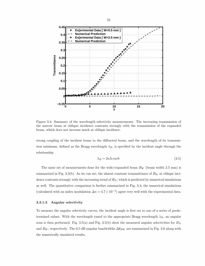
3.4 Summary of the wavelength selectivity measurements. The increasing transmission of

the narrow beam at oblique incidence contrasts strongly with the transmission of the

expanded beam, which does not increase much at oblique incidence. . . . . . . . . . . 24

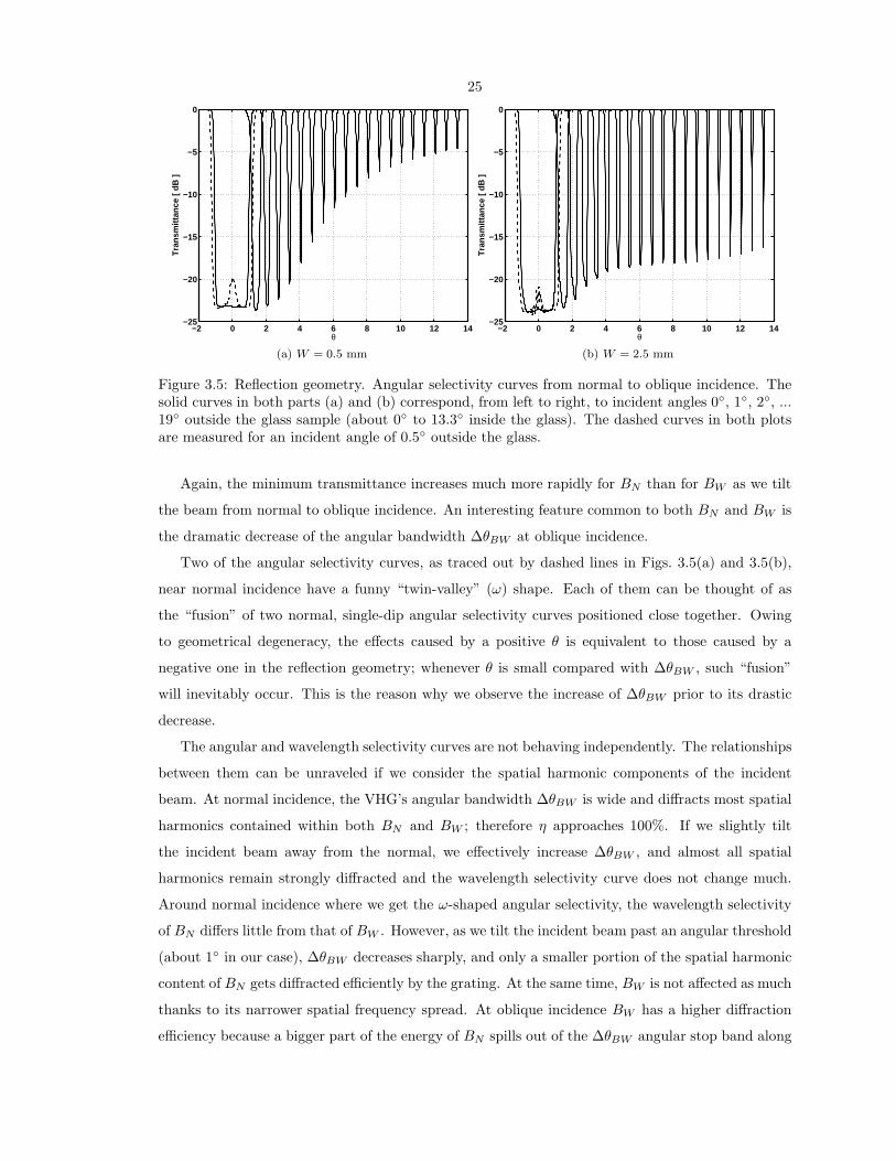
3.5 Reflection geometry. Angular selectivity curves from normal to oblique incidence. The

solid curves in both parts (a) and (b) correspond, from left to right, to incident angles

0◦, 1◦, 2◦, ... 19◦ outside the glass sample (about 0◦ to 13.3◦ inside the glass). The

dashed curves in both plots are measured for an incident angle of 0.5◦ outside the glass. 25

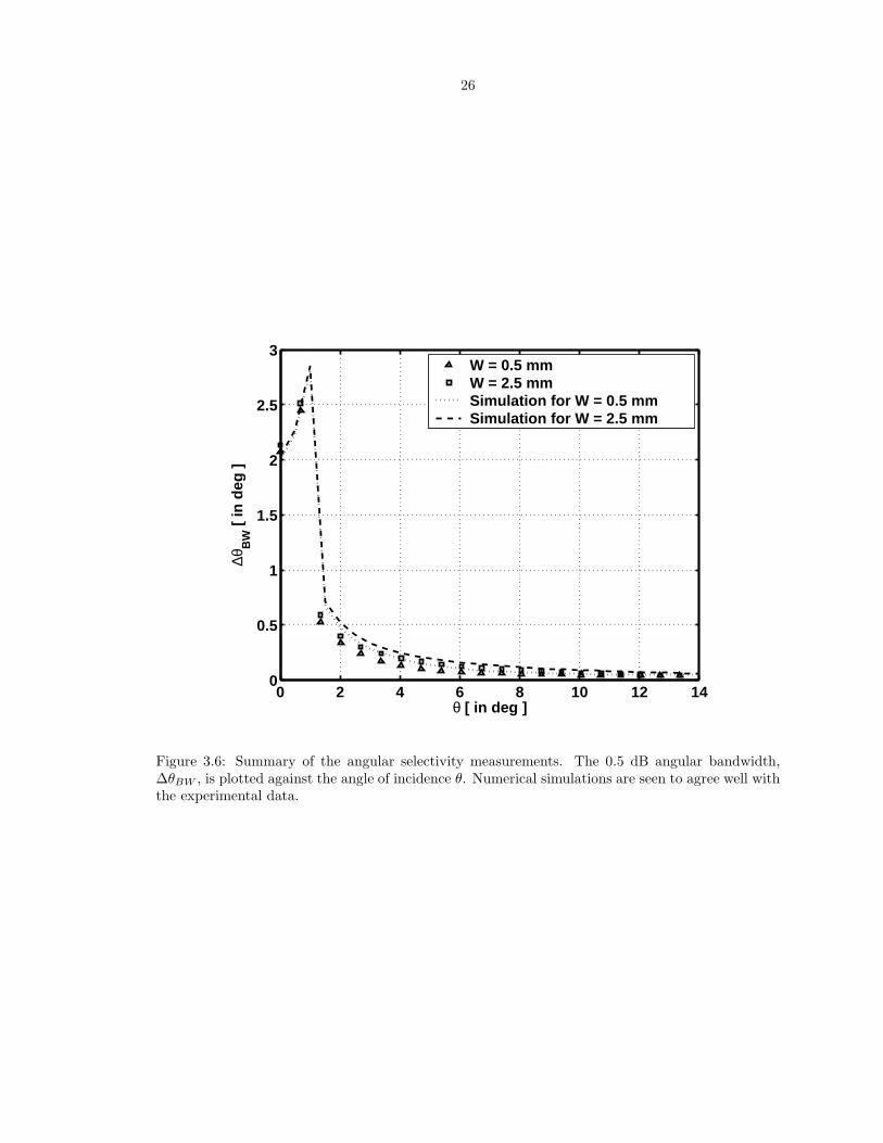
3.6 Summary of the angular selectivity measurements. The 0.5 dB angular bandwidth,

∆θBW , is plotted against the angle of incidence θ. Numerical simulations are seen to

agree well with the experimental data. . . . . . . . . . . . . . . . . . . . . . . . . . . . 26

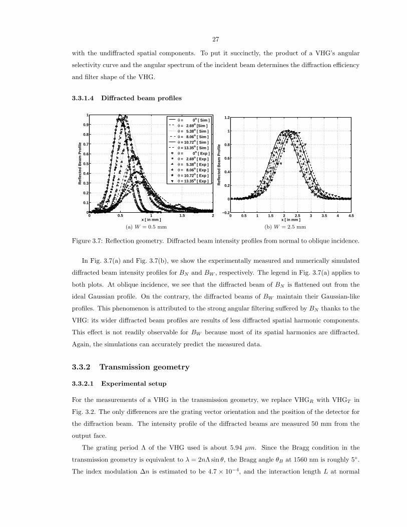
3.7 Reflection geometry. Diffracted beam intensity profiles from normal to oblique incidence. 27

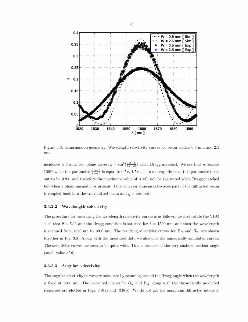
3.8 Transmission geometry. Wavelength selectivity curves for beam widths 0.5 mm and 2.5

mm. . . . . . . . . . . . . . . . . . . . . . . . . . . . . . . . . . . . . . . . . . . . . . . 28

3.9 Transmission geometry. Angular selectivity curves around Bragg angle θB ≈ 5◦. . . . 29

3.10 Normalized diffracted intensity beam profiles in the transmission geometry around

Bragg angle θB ≈ 5◦; ∆θ = θ − θB. All beam profiles are measured 50 mm from the

output face. The circles represent experimental measurements and the dashed lines are

the numerical simulations. . . . . . . . . . . . . . . . . . . . . . . . . . . . . . . . . . . 30

4.1 Recording a holographic grating inside a LiNbO3 crystal at λrec= 488 nm in the trans-

mission geometry and then operating it as a WDM filter in the reflection geometry. . 32

4.2 The athermal design of a holographic filter utilizing an Al-Si composite beam microac-

tuator whose tip deflects as the temperature changes. . . . . . . . . . . . . . . . . . . 34

4.3 Filter response measured in the through channel at θ′B = 5◦ for three different temper-

atures (a) without and (b) with the compensating MEMS mirror. . . . . . . . . . . . 34

4.4 The solid curve represents the calculated optimal compensation angle θ′B as a function

of temperature change ∆T . The dash-dot curve is the measured angular deflection of

the MEMS mirror subject to ∆T . . . . . . . . . . . . . . . . . . . . . . . . . . . . . . 35

xii

4.5 Experimental setup combining the thermally driven MEMS mirror with the recorded

holographic filter to realize the athermal filter design. A picture of the MEMS mirror

is also shown. . . . . . . . . . . . . . . . . . . . . . . . . . . . . . . . . . . . . . . . . . 36

4.6 The Bragg wavelengths measured with the athermal design for three different incident

angles versus temperature. . . . . . . . . . . . . . . . . . . . . . . . . . . . . . . . . . 37

5.1 A schematic graph of a grating in the 90 degree geometry. . . . . . . . . . . . . . . . . 41

5.2 The grating region has been divided into tiny rectangular regions to facilitate numerical

simulation. . . . . . . . . . . . . . . . . . . . . . . . . . . . . . . . . . . . . . . . . . . 43

5.3 Working principle of the numerical simulation. The inherent causality of gratings in

the 90 degree geometry facilitates the algorithm. . . . . . . . . . . . . . . . . . . . . . 44

5.4 Simulated incident (a) and diffracted (b) beam profiles for the Bragg-matched case. . 45

5.5 Simulated incident (a) and diffracted (b) beam profiles for the Bragg mismatch case. . 46

5.6 Normalized diffracted beam intensity profiles for the Bragg-matched (traced out by

crosses) and Bragg-mismatch cases (denoted by squares). The solid curve is plotted

according to the analytical solution of the Bragg-matched case Eq. (5.6), which fits

excellently with our numerical prediction. . . . . . . . . . . . . . . . . . . . . . . . . . 47

5.7 Simulated magnitude response of 90 degree geometry gratings for various index mod-

ulation ∆n. . . . . . . . . . . . . . . . . . . . . . . . . . . . . . . . . . . . . . . . . . . 47

5.8 Experimental setup for monitoring the diffracted beam profile. . . . . . . . . . . . . . 48

5.9 Temporal evolution of the diffracted beam profile formed on the CCD camera. . . . . 49

5.10 The variable x is used in Eq. (5.11) for the calculation of diffracted beam profiles. . . 49

5.11 Theoretical plot of the normalized beam profile for different values of index modulation. 50

5.12 Averaged diffracted beam profile at different temporal points. (Experimental) . . . . . 51

5.13 Temporal evolution of index modulation ∆n derived by fitting the diffracted beam

profile to Eq. (5.12). . . . . . . . . . . . . . . . . . . . . . . . . . . . . . . . . . . . . . 52

5.14 Implementation of a holographic add-drop filter in the 90 degree geometry. . . . . . . 53

5.15 Experimental setup for testing the 90 degree holographic filter. . . . . . . . . . . . . . 54

5.16 Experimental filter response measured in the filter through (transmission) channel.

(This corresponds to an index modulation of ∆n = 6 × 10−5.) . . . . . . . . . . . . . 55

6.1 The temporal resolution in two-pulse pump-and-probe experiments is strongly affected

by the transverse pulse widths and the angle θ between the pulses involved. Optimal

resolution is obtained when the pulses propagate collinearly, as in case (a); deviation

from collinearity causes the resolution to deteriorate due to the transverse dimensions

of the pulses, as in case (b). . . . . . . . . . . . . . . . . . . . . . . . . . . . . . . . . . 58

xiii

6.2 Configuration of a femtosecond holographic experiment in the transmission geometry;

1 and 2 are the pump (recording) pulses, while 3 and 4 are the probe and diffracted

pulses. The ζ- and ξ- axes are parallel and perpendicular to the direction of propagation

of the diffracted probe pulse. . . . . . . . . . . . . . . . . . . . . . . . . . . . . . . . . 59

6.3 Schematic illustration of the holographic pump-and-probe setup. (BC: Berek compen-

sator, serving as half-wave plate for the probe pulse; BS: beam splitter; D: photodetec-

tor; DS: probe delay stage; L: lens; M: mirror; P: polarizer) . . . . . . . . . . . . . . . 64

6.4 Comparison between theory and experiment (θp = 2.77o). Polarization dependence of

the measured diffracted probe trace η(∆t) is shown. The dashed lines are obtained

from the theory. The solid lines are scaled probe pulse intensity profiles. Λ stands for

the grating period. . . . . . . . . . . . . . . . . . . . . . . . . . . . . . . . . . . . . . . 65

6.5 Temporal resolution of the holographic pump-and-probe setup. The dashed curve is

calculated numerically according to the theory; the solid curve is plotted under paraxial

approximation, using Eq. (6.12). The dash-dot curve, drawn here for comparison, is

the temporal resolution for the single-pump-single-probe configuration. . . . . . . . . 66

6.6 The concept of the composite pump. The limited longitudinal dimension of femtosecond

pulses gives rise to a strip-like region of actual overlap whose width is determined by

the pulse temporal duration as well as the angle of intersection, as shown in the lower

part. . . . . . . . . . . . . . . . . . . . . . . . . . . . . . . . . . . . . . . . . . . . . . . 67

7.1 Schematic diagram of a collinear pump-probe experiment; M is a dielectric dichroic

mirror, L is a long-focus (500 mm) lens, F is a band edge filter for the pump light, D

is a photodiode, DS is the probe delay stage. . . . . . . . . . . . . . . . . . . . . . . . 72

7.2 Transmission coeffcient Tp versus peak pump pulse intensity Ip0. The squares, circles

and crosses correspond to the samples 1, 2 and 3, respectively. . . . . . . . . . . . . . 73

7.3 Transverse beam profile (normalized intensities) for different values of the nonlinear

absorption parameter qp = βpIp0d. . . . . . . . . . . . . . . . . . . . . . . . . . . . . . 74

7.4 Dependence of the transmission coefficient Tp on qp = βpIp0d. The dashed curve is

plotted from Eq. (7.3). The squares, circles, and crosses represent the experimental

data for samples 1, 2 and 3, respectively. . . . . . . . . . . . . . . . . . . . . . . . . . 76

7.5 The quadratic absorption coefficient βp of LiNbO3 as function of photon energy. . . . 77

7.6 Transmission coefficient Tr of the probe pulse versus the time delay ∆t for sample 4 and

four different values of the pump intensity. The circles, squares, crosses, and triangles

correspond to Ip0 ∼ 52, 83, 114 and 170 GW/cm2, respectively. . . . . . . . . . . . . . 78

xiv

7.7 Transmission coefficient Tr versus ∆t for different combinations of pump and probe po-

larizations; the first and second characters of each pair in the legend (e.g., “X”) specify

the orientation of the polarization vector of the pump and probe pulses, respectively. . 79

7.8 The pump pulse is passing through a short segment of nonlinear-absorptive medium. . 82

7.9 Dependence of the dip and plateau amplitudes on the product qp = βpIp0d for sample

3 and two different pump-probe polarization states. The points are experimental data,

and the solid lines are theoretical fits. . . . . . . . . . . . . . . . . . . . . . . . . . . . 83

8.1 Schematic illustration of the holographic pump-and-probe setup in LiNbO3. The pump

pulses are polarized perpendicular to the surface of the optical table. The Berek com-

pensator serves as a half-wave plate for the probe pulse; the retro-reflector is mounted

on a translation stage (resolution 1 µm); BS: beam splitter; DS: probe delay stage; L:

lens. . . . . . . . . . . . . . . . . . . . . . . . . . . . . . . . . . . . . . . . . . . . . . . 89

8.2 The measured diffraction efficiency η as a function of the probe delay ∆t in an un-

doped LiNbO3 sample.. The pump pulses are polarized along the c-axis and η‖(η⊥) is

measured when the probe pulses are polarized parallel (perpendicular) to those of the

pump pulses. . . . . . . . . . . . . . . . . . . . . . . . . . . . . . . . . . . . . . . . . . 90

8.3 The measured diffraction efficiency η as a function of the probe delay ∆t in undoped

(circles), iron-doped (triangles) and manganese-doped (squares) LiNbO3 samples. The

pump pulses are polarized along the c-axis, and all measurements are carried out in

the η⊥) configuration. . . . . . . . . . . . . . . . . . . . . . . . . . . . . . . . . . . . . 93

8.4 Configuration of the femtosecond holographic experiment in lithium niobate; 1 and 2

are the pump (recording) pulses, while 3 and 4 are the probe and diffracted pulses. . . 94

8.5 Pump-and-probe data acquired for qp ≈ 1 in a LiNbO3 : Fe sample with thickness 70

µm. The circles denote the experimental data, and the dashed curve is the theoretical

diffraction efficiency plotted according to Eq. (8.6) for n2 = 1.79 × 10−5 cm2/GW. . . 96

8.6 The summary of measured values of ηpeak (in squares) and ηpl. (in triangles) for different

pump intensities in the 70-µm LiNbO3 sample. The pump pulses are polarized along

the c-axis, and all measurements are carried out in the η‖) configuration. . . . . . . . 99

1

Chapter 1

Introduction

In this thesis we investigate the operation of holographic gratings with broadband light sources.

We begin this chapter by introducing some of the important definitions and properties of volume

holographic gratings (VHGs) and then review several interesting properties and applications of

volume holograms in the context of spatial and temporal domains, which are the manifestations of

the selectivity inherent in volume holograms.

For the rest of the thesis, we will devote our attention to the investigation of temporal and

spectral properties of volume holograms by means of polychromatic operations.

1.1 Volume holographic gratings and their filtering proper-

ties

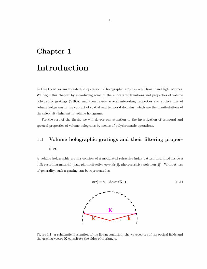
A volume holographic grating consists of a modulated refractive index pattern imprinted inside a

bulk recording material (e.g., photorefractive crystals[1], photosensitive polymers[2]). Without loss

of generality, such a grating can be represented as

n(r) = n + ∆n cosK · r, (1.1)

k k

K

Figure 1.1: A schematic illustration of the Bragg condition: the wavevectors of the optical fields andthe grating vector K constitute the sides of a triangle.

2

where n is the average refractive index of the material and K is the grating vector and is related to

the grating period Λ by |K| = K = 2π/Λ. Once recorded, the grating can act as an efficient coupler

between plane waves. The coupling property is largely specified by two important parameters. The

first is the grating period Λ, which determines the Bragg condition and therefore the appropriate

interacting optical wavelength λ. As shown in Fig. 1.1, if the wavevectors of two optical fields and

the grating vector K constitute the sides of a triangle, the optical fields can be coupled through

the holographic grating when the conservation of momentum and energy is satisfied. The relevant

Bragg condition in this case is

λ = 2nΛ cos θ, (1.2)

where θ is the angle of incidence. Plane wave components that meet the Bragg condition will be

diffracted by the grating and those that do not will be transmitted instead. Therefore the holographic

grating can act as a filter, discriminating between various plane wave components based on the Bragg

condition.

k1

k2

K

k

k1

k2

K

k

(a) Bragg-matched case. (b) Bragg-mismatch case

Figure 1.2: Angular selectivity of a volume hologram.

1.2 Spatial-domain perspective

The angular selectivity of volume holograms is responsible for their various applications in the

spatial domain. The principle can be explained with the help of Fig. 1.2. In Fig. 1.2(a) we show the

Bragg-matched case where the conservation of momentum is satisfied and most of the incident light

(with wavevector k1) is coupled into the diffracted light (with wavevector k2). Also shown is the

k-diagram of this particular configuration and the selectivity curve of the grating, which represents

3

the diffraction efficiency η of the VHG as a function of the phase mismatch ∆k defined as

∆k = k2 − k1 − K. (1.3)

In the Bragg-matched case, ∆k = 0 and we achieve maximum, in this case 100%, energy coupling.

If now we change the incident angle, as shown in Fig. 1.2(b), a corresponding change (tilting)

of k2 comes about as a result, giving rise to a nonzero phase mismatch denoted by the horizontal

double-headed arrow. The diffraction efficiency will therefore decrease; in this case η happens to be

0, and no beam coupling will be observed. In general, the longer the interaction length between the

grating and the light field is, the more selective the VHG will be.

Various spatial-domain properties and applications of holograms are attributed to their angular

selectivity; for instance, angle multiplexing[3], shift multiplexing[4], holographic storage[5], image

processing[6] and pattern recognition, to name just a few.

k1

k2

K

k

K

kk1

k2

(a) Bragg-matched case. (b) Bragg-mismatch case

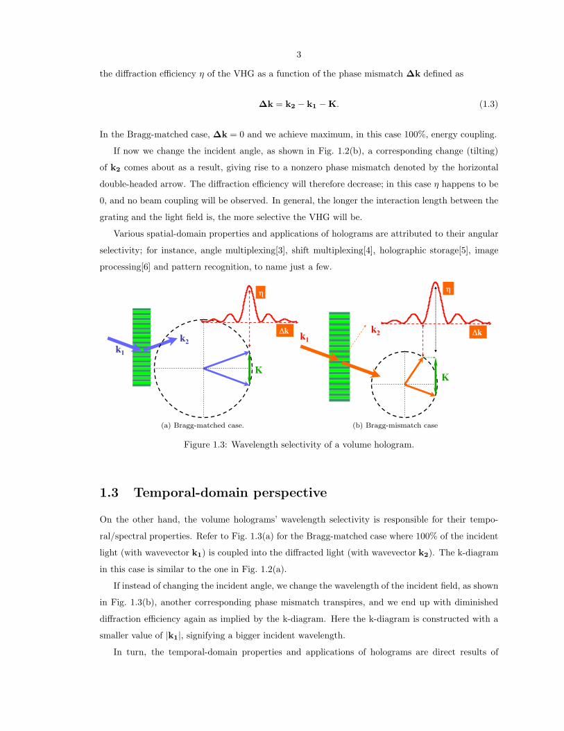
Figure 1.3: Wavelength selectivity of a volume hologram.

1.3 Temporal-domain perspective

On the other hand, the volume holograms’ wavelength selectivity is responsible for their tempo-

ral/spectral properties. Refer to Fig. 1.3(a) for the Bragg-matched case where 100% of the incident

light (with wavevector k1) is coupled into the diffracted light (with wavevector k2). The k-diagram

in this case is similar to the one in Fig. 1.2(a).

If instead of changing the incident angle, we change the wavelength of the incident field, as shown

in Fig. 1.3(b), another corresponding phase mismatch transpires, and we end up with diminished

diffraction efficiency again as implied by the k-diagram. Here the k-diagram is constructed with a

smaller value of |k1|, signifying a bigger incident wavelength.

In turn, the temporal-domain properties and applications of holograms are direct results of

4

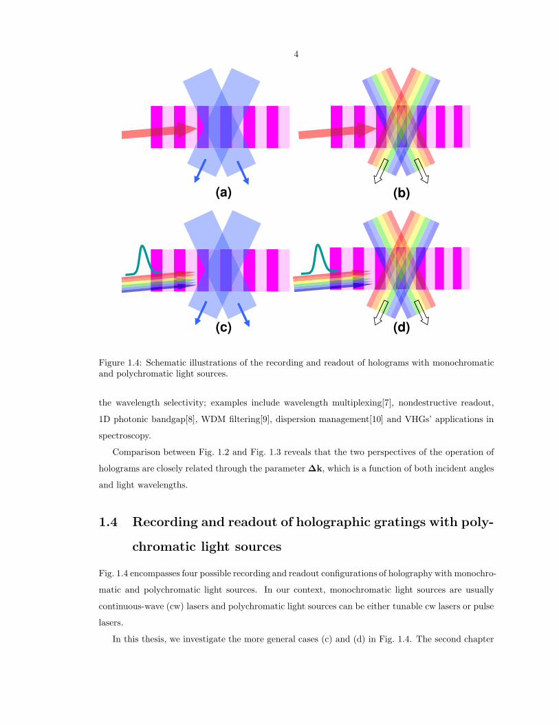
(a) (b)

(c) (d)

Figure 1.4: Schematic illustrations of the recording and readout of holograms with monochromaticand polychromatic light sources.

the wavelength selectivity; examples include wavelength multiplexing[7], nondestructive readout,

1D photonic bandgap[8], WDM filtering[9], dispersion management[10] and VHGs’ applications in

spectroscopy.

Comparison between Fig. 1.2 and Fig. 1.3 reveals that the two perspectives of the operation of

holograms are closely related through the parameter ∆k, which is a function of both incident angles

and light wavelengths.

1.4 Recording and readout of holographic gratings with poly-

chromatic light sources

Fig. 1.4 encompasses four possible recording and readout configurations of holography with monochro-

matic and polychromatic light sources. In our context, monochromatic light sources are usually

continuous-wave (cw) lasers and polychromatic light sources can be either tunable cw lasers or pulse

lasers.

In this thesis, we investigate the more general cases (c) and (d) in Fig. 1.4. The second chapter

5

introduces the matrix formulation for the analysis of VHGs in the reflection geometry, which will

be used in the next three chapters. Chapters 3, 4 and 5 are then devoted to the case (c) where a

uniform holographic grating is recorded by two interfering monochromatic fields and then read out

with a continuously tunable laser source. Photosensitive glass and lithium niobate (LiNbO3) will be

our materials of choice.

In the last three chapters we will concern ourselves with case (d), where gratings are recorded

and read out by femtosecond pulse sources; we will discuss several observed nonlinear phenomena in

the regime of femtosecond holography. Experiments are conducted in calcium fluoride (CaF2) and

lithium niobate samples.

6

Bibliography

[1] G. C. Valley, M. B. Klein, R. A. Mullen, D. Rytz, and B. Wechsler. Photorefractive materials.

Annual Review of Materials Science, 18:165–188, 1988.

[2] J. E. Ludman, J. R. Riccobono, N. O. Reinhand, I. V. Semenova, Y. L. Korzinin, S. M. Shahriar,

H. J. Caulfield, J. M. Fournier, and P. Hemmer. Very thick holographic nonspatial filtering of

laser beams. Optical Engineering, 36(6):1700–1705, June 1997.

[3] F. H. Mok. Angle-multiplexed storage of 5000 holograms in lithium niobate. Optics Letters,

18(11):915–917, June 1993.

[4] D. Psaltis, M. Levene, A. Pu, and G. Barbastathis. Holographic storage using shift multiplexing.

Optics Letters, 20(7):782–784, April 1995.

[5] D. Psaltis and F. Mok. Holographic memories. Scientific America, 273:70–76, November 1995.

[6] W. Liu, G. Barbastathis, and D. Psaltis. Volume holographic hyperspectral imaging. Applied

Optics, 43(18):3581–3599, June 2004.

[7] G. A. Rakuljic, V. Leyva, and A. Yariv. Optical data storage by using orthogonal wavelength-

multiplexed volume holograms. Optics Letters, 17(20):1471–1473, October 1992.

[8] J. D. Joannopoulos, P. R. Villenueve, and S. Fan. Photonic crystals: putting a new twist on

light. Nature, 386:143–149, March 1997.

[9] G. A. Rakuljic and V. Leyva. Volume holographic narrow-band optical filter. Optics Letters,

18:459–461, March 1993.

[10] K. O. Hill and G. Meltz. Fiber bragg grating technology fundamentals and overview. Journal

of Lightwave Technology, 15(8):1263–1276, August 1997.

7

Chapter 2

Matrix formulation for holographic

filters in the reflection geometry

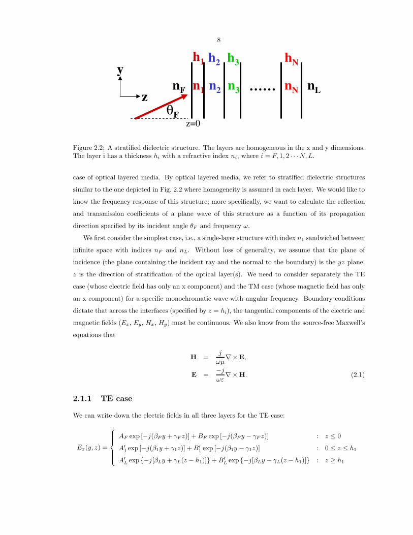
In this chapter, we will introduce a powerful analytical tool, matrix formulation, for volume holo-

grams in the reflection geometry. We will then apply the matrix formulation to the sinusoidal grating

structure as illustrated in Fig. 2.1. Sinusoidal index modulation has a fundamental importance be-

cause any profile of index modulation can be represented as the linear combination thereof by means

of Fourier transform. The ability to analyze such structures will play an important part in the next

two chapters.

2.1 Matrix formulation for optical layered media

The well-established coupled mode analysis[1, 2] gives an accurate description of volume holographic

gratings in the vicinity of the Bragg condition and is highly useful for the characterization of one

dimensional photonic bandgap; however, it is not applicable away from Bragg condition; moreover,

it can not deal with the cases of chirped gratings due to an implicit assumption in the analysis that

only a number of propagating modes are strongly coupled by the grating structure. A more flexible

method will be investigated here.

Before dealing with the sinusoidal grating structure, we first consider the more straightforward

y

z

nL

nF

n(z)=n+ ncosKz

Figure 2.1: A sinusoidal grating structure.

8

……n1 n2 n3 nN nLnF

h1 h2 h3 hN

F

z

y

z=0

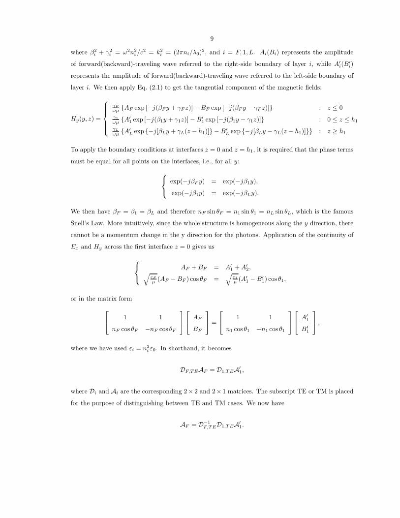
Figure 2.2: A stratified dielectric structure. The layers are homogeneous in the x and y dimensions.The layer i has a thickness hi with a refractive index ni, where i = F, 1, 2 · · ·N, L.

case of optical layered media. By optical layered media, we refer to stratified dielectric structures

similar to the one depicted in Fig. 2.2 where homogeneity is assumed in each layer. We would like to

know the frequency response of this structure; more specifically, we want to calculate the reflection

and transmission coefficients of a plane wave of this structure as a function of its propagation

direction specified by its incident angle θF and frequency ω.

We first consider the simplest case, i.e., a single-layer structure with index n1 sandwiched between

infinite space with indices nF and nL. Without loss of generality, we assume that the plane of

incidence (the plane containing the incident ray and the normal to the boundary) is the yz plane;

z is the direction of stratification of the optical layer(s). We need to consider separately the TE

case (whose electric field has only an x component) and the TM case (whose magnetic field has only

an x component) for a specific monochromatic wave with angular frequency. Boundary conditions

dictate that across the interfaces (specified by z = hi), the tangential components of the electric and

magnetic fields (Ex, Ey, Hx, Hy) must be continuous. We also know from the source-free Maxwell’s

equations that

H =j

ωµ∇× E,

E =−j

ωε∇× H. (2.1)

2.1.1 TE case

We can write down the electric fields in all three layers for the TE case:

Ex(y, z) =

AF exp [−j(βF y + γF z)] + BF exp [−j(βF y − γF z)] : z ≤ 0

A′1 exp [−j(β1y + γ1z)] + B′

1 exp [−j(β1y − γ1z)] : 0 ≤ z ≤ h1

A′L exp {−j[βLy + γL(z − h1)]} + B′

L exp {−j[βLy − γL(z − h1)]} : z ≥ h1

9

where β2i + γ2

i = ω2n2i /c2 = k2

i = (2πni/λ0)2, and i = F, 1, L. Ai(Bi) represents the amplitude

of forward(backward)-traveling wave referred to the right-side boundary of layer i, while A′i(B

′i)

represents the amplitude of forward(backward)-traveling wave referred to the left-side boundary of

layer i. We then apply Eq. (2.1) to get the tangential component of the magnetic fields:

Hy(y, z) =

γF

ωµ {AF exp [−j(βF y + γF z)] − BF exp [−j(βF y − γF z)]} : z ≤ 0

γ1

ωµ {A′1 exp [−j(β1y + γ1z)] − B′

1 exp [−j(β1y − γ1z)]} : 0 ≤ z ≤ h1

γL

ωµ {A′L exp {−j[βLy + γL(z − h1)]} − B′

L exp {−j[βLy − γL(z − h1)]}} : z ≥ h1

To apply the boundary conditions at interfaces z = 0 and z = h1, it is required that the phase terms

must be equal for all points on the interfaces, i.e., for all y:

exp(−jβF y) = exp(−jβ1y),

exp(−jβ1y) = exp(−jβLy).

We then have βF = β1 = βL and therefore nF sin θF = n1 sin θ1 = nL sin θL, which is the famous

Snell’s Law. More intuitively, since the whole structure is homogeneous along the y direction, there

cannot be a momentum change in the y direction for the photons. Application of the continuity of

Ex and Hy across the first interface z = 0 gives us

AF + BF = A′1 + A′

2,√

εF

µ (AF − BF ) cos θF =√

ε1

µ (A′1 − B′

1) cos θ1,

or in the matrix form

1 1

nF cos θF −nF cos θF

AF

BF

=

1 1

n1 cos θ1 −n1 cos θ1

A′1

B′1

,

where we have used εi = n2i ε0. In shorthand, it becomes

DF,TEAF = D1,TEA′1,

where Di and Ai are the corresponding 2× 2 and 2× 1 matrices. The subscript TE or TM is placed

for the purpose of distinguishing between TE and TM cases. We now have

AF = D−1F,TED1,TEA′

1.

10

Obviously, the same relationship will transpire at the interface z = h1 as well:

A1 = D−11,TEDL,TEA′

L.

We therefore reach the conclusion that the matrix D−1i,TEDi+1,TE takes care of the interface effect

between layers i and i+1.

Now let us account for the relationship between A′i and Ai. Since

A′1 exp [−j(β1y + γ1z)] + B′

1 exp [−j(β1y − γ1z)]

and

A1 exp {−j[β1y + γ1(z − h1)]} + B1 exp {−j[β1y − γ1(z − h1)]}

are just two expressions of the same electric field in layer i, they must be equal. By equating the

two expressions we get

A′1 =

A′1

B′1

=

exp(jφ1) 0

0 exp(−jφ1)

A1

B1

= P1A1,

where φ1 = γ1h1 = k1 cos θ1h1. It is conspicuous that the matrix Pi takes care of the propagation

effect inside layer i with thickness hi. Now, rather straightforwardly, we may write down

AF = D−1F,TED1,TEP1D−1

1,TEDL,TEA′L = D−1

F,TEM1,TEDL,TEA′L, (2.2)

where

M1,TE =

cosφ1j sin φ1

n1 cos θ1

jn1 cos θ1 sin φ1 cosφ1

is the layer matrix of dielectric layer 1 for TE wave propagation and, interestingly, |M1,TE |. We

point out that all layer matrices are unimodular.

2.1.2 TM case

In the TE case we derive the layer matrices for field components Ex and Hy, while in the TM case

we turn to Ey and Hx. Following a procedure similar to that in the TE case, we have

Di,TM =

cos θi cos θi

ni −ni

11

and the layer matrix

Mi,TM =

cosφij cos θi sin φi

ni

jni sin φi

cos θicosφi

for TM waves. Just as in the TE case, Mi,TM is unimodular.

2.1.3 Diffraction efficiency of a multilayer medium

Now that we have accounted for the effects of interfaces and propagation, we are ready to handle

the configuration as shown in Fig. 2.2. We can directly write down

AF = D−1F M1M2 · · ·MNDLA′

L, (2.3)

where Di and Mi are the corresponding interface and layer matrices for TE or TM waves. In either

case, Eq. (2.3) can be simplified and recast as

AF

BF

= J

A′L

B′L

=

J11 J12

J21 J22

A′L

B′L

.

The reflection coefficient is r = BF /AF = J21/J11 and the transmission coefficient is t = A′L/AF =

1/J11, where B′L = 0 has been adopted because the electromagnetic radiation is incident from the

left side and there is no backward travelling wave in the rightmost medium. The coefficients r and

t are in general complex. The reflectance of such a structure is defined as

R = −SFB · az

SFA · az

=|BF |2|AF |2

= |r|2, (2.4)

where SFB (SFA) stands for the Poynting vector of the forward (backward) travelling wave in the

leftmost medium. Similarly, the transmittance is defined as

T =SLA · az

SFA · az

=nL cos θL|A′

L|2nF cos θF |AF |2

= |t|2 nL cos θL

nF cos θF. (2.5)

If the indices of the dielectric layers are all real, there will be no loss and therefore R + T = 1.

2.2 Matrix formulation for sinusoidal gratings

Now we can deal with the sinusoidal grating structure as drawn in Fig. 2.1. The trick is to “slice”

a single period (length Λ) of the grating into L layers, as illustrated in Fig. 2.3. By approximating

each layer as homogeneous with the value of the refractive index at its center, we wind up with the

effective transfer matrix of a single period: C = M1M2 · · ·ML.

12

, L layers

n(z)=n+ ncosKz

…… …………

Figure 2.3: The “slicing” of a single period of a sinusoidal grating structure.

0 10 20 30 40 5010

-9

10-8

10-7

10-6

10-5

10-4

10-3

L

RM

S(

CL

+1-C

L)

Figure 2.4: Convergence of the effective matrix C of a single grating period Λ.

13

It is conceivable that the finer we slice the period, the closer the effective matrix will be to the

“real” transfer matrix of a single period. Let’s say CL is the effective matrix obtained by slicing a

single grating period Λ into L layers. Fig. 2.4 shows that as we increase L, the effective matrix CL

converges. There RMS(CL+1 − CL) stands for the root-mean-square value of the four elements of

the difference between matrices CL+1 and CL.

If the grating has N periods in total, we shall get

AF = D−1F CNDLA′

L

and we may then calculate the reflection and transmission coefficients. This method is computation-

ally favorable because of the fact that the determinant of C is 1; it greatly facilitates the calculation

of the matrix CN :

C =

C11 C12

C21 C22

⇔ CN =

C11UN−1(a) − UN−2(a) C12UN−1(a)

C21UN−1(a) C22UN−1(a) − UN−2(a)

where a = (C11 + C22)/2 and

UN (a) =1√

1 − a2sin[(N + 1) arccos(a)]

is known as the Chebyshev polynomial of the second kind[3].

In Fig. 2.5, we simulate the reflectance, according to Eq. (2.4), of two gratings at normal incidence

(therefore TE and TM cases are degenerate). The index modulation is the same for the two gratings

(∆n = 4×10−4), while the medium (LiNbO3 in this case) lengths are 0.5 cm and 2 cm, respectively.

The number of slices for a single period is 35.

The bandgap centered at the Bragg wavelength 1550 nm is about 0.14 nm (corresponding to

about 17.5 GHz), and it is not affected much by the sample length. This phenomenon can also

be explained by the coupled mode analysis: within the bandgap of the filter, κ > |∆β|. Since κ is

determined by the index modulation, the sample length should not affect the filter bandwidth. In the

context of Bloch formalism[4], the range of frequency components that possess complex propagation

constants is also determined by the index modulation.

We also observe local maxima and minima outside the bandgap. These “ripples” occur more

frequently on the wavelength axis for a longer sample. To explain this, we can think of the grating

as a collection of numerous mirrors distributed along the z-axis. If the optical path length inside

the sample is an integral multiple of a half wavelength, i.e., n1h1 = mλ/2 where m is an integer,

the reflection from the distributed mirrors will cancel out exactly, and this is the location of a local

minima. Simple calculation shows that the difference between optical frequencies of the adjacent

14

n1=4 10-4

L=2cm

L=0.5cm

1549.6 1549.8 1550 1550.2 1550.40

0.2

0.4

0.6

0.8

1

wavelength ( in nm )

Re

fle

cta

nc

e

Figure 2.5: Simulated grating reflectance as a function of incident wavelength (wavelength selectiv-ity) for ∆n = 4 × 10−4. The dotted curve is obtained for a sample length of 2 cm; the solid curve,0.5 cm.

L=2cm

n1=4 10-4

n1=1 10-4

n1=2.5 10-5

1549.6 1549.8 1550 1550.2 1550.40

0.2

0.4

0.6

0.8

1

wavelength ( in nm )

Re

fle

cta

nc

e

Figure 2.6: Simulated grating reflectance as a function of incident wavelength (wavelength selectiv-ity) for a sample length of 2 cm. The dotted curve is obtained for an index modulation ∆n = 4×10−4;the dashed curve, ∆n = 1 × 10−4; the solid curve, ∆n = 2.5 × 10−5.

15

minima satisfy ∆ν = c/2n1h1. Therefore the longer the crystal is, the more frequent is the ripple

oscillation.

In Fig. 2.6, we show simulations for three gratings with different index modualtion but the same

sample length. The bandgaps grow with increasing ∆n, but the frequencies of the out-of-band

oscillation are the same for all three gratings.

2.3 Experimental results

c-axis

recrec

tar

L

y

z

krec

ktar

Kgrating

kreckrec

(a) Recording and readout geometry. (b) The corresponding K-diagram

Figure 2.7: Recording a holographic grating in the transmission geometry and reading it out in thereflection geometry as a WDM filter.

2.3.1 Recording holographic WDM filters in reflection geometry in LiNbO3

As shown in Fig. 2.7(a), we record a holographic grating in the transmission geometry and read out

from the side. By properly choosing the half angle θ between the recording beams, we can control

the (target) Bragg wavelength λtar when the grating is operated in the reflection geometry.

According to the K-diagram depicted in Fig. 2.7(b),

2ktar = Kgrating = 2krec sin θ =⇒ θ = arcsin

(

ntarλrec

λtar

)

.

In our experiment, the parameters are as follows:

16

Recording Time ( in min. )

Dif

fra

ctio

n E

ffic

ien

cy

0 50 100 1500

0.2

0.4

0.6

0.8

1

Figure 2.8: A recording curve of the holographic grating. (A stabilization system is incorporatedinto the recording setup for optimal stability.)

• The target readout wavelength at normal incidence λtar = 1550 nm.

• The recording wavelength λrec = 514.5 nm.

• The refractive index ntar of the medium at λtar. We use LiNbO3 samples in our experiment

and ntar = 2.2116.

• The half angle between the recording beams (outside the LiNbO3 sample) is calculated to be

47.23◦.

A typical recording curve is shown in Fig. 2.8. A stabilization system has been incorporated

into the system, and a piezo mirror is introduced to adjust the optical path of one of the recording

beams in order to optimize the recording process. The “over-the-hump” behavior is rather obvious,

and the modulation depth of the refractive index ∆n is estimated to be 3.26 × 10−4.

2.3.2 Measured filter response

The measured transmittance at normal incidence as a function of the incident wavelengths is plotted

in Fig. 2.9. The Bragg wavelength (center wavelength) of the filter is estimated to be 1563.6 nm with

a bandwidth of 0.115 nm (about 14.5 GHz). The criterion used to calculate them is as follows: we

first find the two points of the filter whose through-channel transmittances are 0.5 dB higher than

17

( in nm )

DE

( T

hru

ch

an

nel

, in

dB

)

1563.4 1563.5 1563.6 1563.7 1563.8 1563.9-22

-20

-18

-16

-14

-12

-10

-8

-6

-4

-2

0

Figure 2.9: Measured filter transmittance in the through channel.

the minimum transmittance (that is, about 90% reflectance); they are defined as the edges of the

filter stopband; Bragg wavelength is then calculated as the average of the two edge wavelengths, and

the bandwidth is the difference between them. As we can see, the Bragg wavelength is not exactly

the target wavelength we have designed. This indicates that the angle θ in the experimental setup

can be slightly different from the theoretical value.

18

Bibliography

[1] H. Kogelnik. Coupled wave theory for thick hologram gratings. Bell System Technical Journal,

48(9):2909–2947, November 1969.

[2] A. Yariv. Optical electronics in modern communications. Oxford University Press, New York,

5th edition, 1997.

[3] Max Born and Emil Wolf. Principles of Optics. Cambridge, London, 7th edition, 1999.

[4] A. Yariv and P. Yeh. Optical Waves in Crystals. John Wiley & Sons, New York, 1984.

19

Chapter 3

Beam-width dependent filtering

properties of volume holographic

gratings

The finite dimension of the incident beam used to read out volume holographic gratings has interest-

ing effects on their filtering properties. As the readout beam gets narrower, there is more deviation

from the ideal response predicted for monochromatic plane waves. In this chapter, we experimentally

explore some beam-width-dependent phenomena such as wavelength selectivities, angular selectiv-

ities and diffracted beam profiles. Volume gratings in both reflection and transmission geometries

are investigated near 1550 nm. Numerical simulations utilizing the technique of Fourier decomposi-

tion provide satisfactory explanation and confirm that the spread of spatial harmonics is the main

contributing factor.

3.1 Introduction

The coupling effects between plane waves mediated by VHGs has been treated rigorously before

using various theoretical approaches, e.g., coupled-mode analysis[1, 2] and matrix formulation as

discussed in the previous chapter. We will use these well-established results as given for our numerical

simulations in this chapter.

Unlike thin gratings, VHGs are very sensitive to phase mismatch because of less ambiguity al-

lowed in the momentum space. Thanks to its excellent selectivity, VHGs have become an ideal candi-

date for various promising technological applications such as neural networks[3], optical correlators[4]

and holographic data storage[5, 6]. VHGs also prove useful in telecommunications. Essentially a

one-dimensional photonic crystal when ∆n is appreciable (∆n ≥ 10−4), holographic gratings in the

reflection geometry can serve as superior filters[7, 8] for wavelength division multiplexing (WDM)

thanks partly to their low crosstalk and readily engineered bandwidths.

The versatility of VHGs provides the motivation behind our work presented here. In this chapter,

20

x

z

xÕ

zÕ

!

E(x,y,z)

EÕ(x,y,z)

VHGR

VHGT

Figure 3.1: Theoretical configuration. The volume holographic grating has a transfer functionH(ki;kd). VHGR/T is a volume holographic grating in the reflection/transmission geometry.

we show the experimentally measured beam-width dependence of the wavelength selectivity, angular

selectivity and diffracted beam profiles of VHGs in both the reflection and transmission geometries

for s-polarized fields. With the help of Fourier analysis, we can satisfactorily explain the interesting

discrepancies between the experimental data and the ideal results predicted for plane waves.

3.2 Theoretical consideration

In Fig. 3.1, we consider how a VHG affects a monochromatic incident optical field whose complex

amplitude is Ei(x, y, z). The length of the grating measures L along z-axis and is assumed to be

infinite in the other two dimensions. With the knowledge of f(x, y) = Ei(x, y, z = 0), the complex

amplitude Ei(x, y, z) can be uniquely determined by the diffraction integral in the case of propagation

in a homogeneous medium:

Ei(x, y, z) =

∫∫

F (kix, kiy)exp[−j(kixx + kiyy + kizz)]dkix

2π

dkiy

2π, (3.1)

where ki = |ki| =√

k2ix + k2

iy + k2iz is the wavenumber of the monochromatic radiation and F (kix, kiy)

is the 2D Fourier transform of f(x, y). Each F (kix, kiy) represents a constituent plane-wave (or an-

gular) component of Ei(x, y, z). Basic Fourier transform relationships tell us that the narrower

the incident beam is, the more spread-out its angular components will be. The “non-planeness” of

Ei(x, y, z) can be thought of as a natural manifestation of the linear combination of all plane wave

elements F (kix, kiy)e−jki·r. For an obliquely incident optical field (tilted by θ), such as E′i(x, y, z)

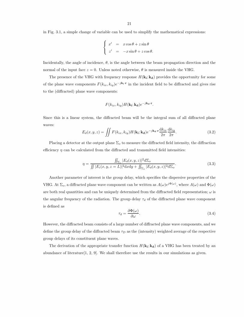
21

in Fig. 3.1, a simple change of variable can be used to simplify the mathematical expressions:

x′ = x cos θ + z sin θ

z′ = −x sin θ + z cos θ.

Incidentally, the angle of incidence, θ, is the angle between the beam propagation direction and the

normal of the input face z = 0. Unless noted otherwise, θ is measured inside the VHG.

The presence of the VHG with frequency response H(ki;kd) provides the opportunity for some

of the plane wave components F (kix, kiy)e−jki·r in the incident field to be diffracted and gives rise

to the (diffracted) plane wave components:

F (kix, kiy)H(ki;kd)e−jkd·r.

Since this is a linear system, the diffracted beam will be the integral sum of all diffracted plane

waves:

Ed(x, y, z) =

∫∫

F (kix, kiy)H(ki;kd)e−jkd·rdkix

2π

dkiy

2π. (3.2)

Placing a detector at the output plane Σo to measure the diffracted field intensity, the diffraction

efficiency η can be calculated from the diffracted and transmitted field intensities:

η =

∫∫

Σo|Ed(x, y, z)|2dΣo

∫∫

|Ei(x, y, z = L)|2dxdy +∫∫

Σo|Ed(x, y, z)|2dΣo

. (3.3)

Another parameter of interest is the group delay, which specifies the dispersive properties of the

VHG. At Σo, a diffracted plane wave component can be written as A(ω)ejΦ(ω), where A(ω) and Φ(ω)

are both real quantities and can be uniquely determined from the diffracted field representation; ω is

the angular frequency of the radiation. The group delay τd of the diffracted plane wave component

is defined as

τd =∂Φ(ω)

∂ω. (3.4)

However, the diffracted beam consists of a large number of diffracted plane wave components, and we

define the group delay of the diffracted beam τD as the (intensity) weighted average of the respective

group delays of its constituent plane waves.

The derivation of the appropriate transfer function H(ki;kd) of a VHG has been treated by an

abundance of literature[1, 2, 9]. We shall therefore use the results in our simulations as given.

22

L

!

Ddiff

Dtr

RB

VHGR

EXP(5�)

TL

VHGT

RS

L

Figure 3.2: Experimental setup. TL: tunable laser source (from 1520 nm to 1600 nm); EXP(5×):beam expander; VHGR/T: volume holographic grating in the reflection/transmission geometry;Dtr/diff : detector for the transmitted/diffracted beam; RS: rotational stage; RB: razor blade con-trolled by a translation stage for measurement of the diffracted beam profile.

3.3 Numerical simulations and experimental results

In this section, we present the experimental results and numerical simulations of VHGs in the

reflection and transmission geometries separately. In all cases, the electric fields are perpendicular

to the plane of incidence (s-polarized). For each geometry, we first describe the experimental setup

and then compare the measurements and theoretical predictions for two different beam widths. All

VHGs used are provided by Ondax Inc. and recorded in photosensitive glass plates. The absorption

inside the glass of the wavelengths used is negligible.

3.3.1 Reflection geometry

In telecommunication, WDM filters are needed to select and/or manipulate a desired wavelength

from a bank of available channels. In reconfigurable communication systems, tunable optical filters

play an increasingly important part. Examples include tunable arrayed waveguide gratings (AWG)

[10], wavelength tuning based on varying temperature [11] and the application of stress [12]. Tunable

filters have also been realized in reflection-geometry VHGs by means of angular tuning[13]. To

appreciate and efficiently utilize this filtering configuration, it is important to know how oblique

incidence impacts the filtering properties.

23

3.3.1.1 Experimental setup

The experimental setup is schematically shown in Fig. 3.2; a reflection-geometry VHG, denoted by

VHGR, whose grating period Λ is about 532 nm (the corresponding Bragg wavelength at normal

incidence is about 1581 nm) is mounted on a rotational stage for precise angular control. The

light from a tunable laser source (tuning range 1520 nm ∼ 1600 nm) is channeled through a fiber

collimator (Newport model f-col-9-15) and then used to conduct measurements. The interaction

length at normal incidence L is 14 mm. The output laser beam profile from the collimator is

Gaussian with a diameter of 0.5 mm, which is the spatial width across its intensity profile where

it drops to 1/e2 of the peak value. A beam expander (5×) consisting of two cylindrical lenses (a

negative lens with focal length -15 mm and a positive lens whose focal length is 75 mm) can be

moved in to widen the incident beam. The angular spread of the (un-)expanded beam is calculated

to be (0.15◦)0.03◦ inside the glass, corresponding to (0.225◦)0.045◦ in the air.

For each incident angle θ and wavelength λ of interest, the power of both the transmitted and

diffracted beams are monitored, from which the diffraction efficiency can be calculated. A razor

blade motion-controlled by a translation stage can be moved across the diffracted beam to measure

its intensity profile. The distance between the razor blade and the output face is about 50 mm.

3.3.1.2 Wavelength selectivity

1535 1540 1545 1550 1555 1560 1565 1570 1575 1580 1585−25

−20

−15

−10

−5

0

λ [ nm ]

Tra

nsm

ittan

ce [

dB ]

1535 1540 1545 1550 1555 1560 1565 1570 1575 1580 1585−25

−20

−15

−10

−5

0

λ [ nm ]

Tra

nsm

ittan

ce [

dB ]

(a) W = 0.5 mm (b) W = 2.5 mm

Figure 3.3: Reflection geometry. Wavelength selectivity curves from normal to oblique incidence.The measured curves in both parts (a) and (b) correspond, from right to left, to incident angles 0◦,1◦, 2◦, ... 19◦ outside the glass sample (about 0◦ to 13.3◦ inside the glass).

To measure wavelength selectivity curves, the incident angle θ is first set to one of a series of

predetermined values, from 0◦ to 13.3◦, and then a wavelength scan is carried out. Fig. 3.3(a)

shows the results obtained with the narrow/unexpanded beam BN (beam width W = 0.5 mm);

the transmittance (= 1 − η) curves are plotted out in dB. Each valley-like feature corresponds to

24

0 5 10 15 20−0.05

0

0.05

0.1

0.15

0.2

0.25

0.3

0.35

0.4

0.45

θ

Tra

nsm

ittan

ce

Ex[erimental Data [ W=0.5 mm ]Numerical PredictionEx[erimental Data [ W=2.5 mm ]Numerical Prediction

Figure 3.4: Summary of the wavelength selectivity measurements. The increasing transmission ofthe narrow beam at oblique incidence contrasts strongly with the transmission of the expandedbeam, which does not increase much at oblique incidence.

strong coupling of the incident beam to the diffracted beam, and the wavelength of its transmis-

sion minimum, defined as the Bragg wavelength λB, is specified by the incident angle through the

relationship

λB = 2nΛ cos θ. (3.5)

The same set of measurements done for the wide/expanded beam BW (beam width 2.5 mm) is

summarized in Fig. 3.3(b). As we can see, the almost constant transmittance of BW at oblique inci-

dence contrasts strongly with the increasing trend of BN , which is predicted by numerical simulations

as well. The quantitative comparison is further summarized in Fig. 3.4; the numerical simulations

(calculated with an index modulation ∆n = 4.7× 10−4) agree very well with the experimental data.

3.3.1.3 Angular selectivity

To measure the angular selectivity curves, the incident angle is first set to one of a series of prede-

termined values. With the wavelength tuned to the appropriate Bragg wavelength λB , an angular

scan is then performed. Fig. 3.5(a) and Fig. 3.5(b) show the measured angular selectivities for BN

and BW , respectively. The 0.5 dB angular bandwidths ∆θBW are summarized in Fig. 3.6 along with

the numerically simulated results.

25

−2 0 2 4 6 8 10 12 14−25

−20

−15

−10

−5

0

θ

Tra

nsm

ittan

ce [

dB ]

−2 0 2 4 6 8 10 12 14−25

−20

−15

−10

−5

0

θ

Tra

nsm

ittan

ce [

dB ]

(a) W = 0.5 mm (b) W = 2.5 mm

Figure 3.5: Reflection geometry. Angular selectivity curves from normal to oblique incidence. Thesolid curves in both parts (a) and (b) correspond, from left to right, to incident angles 0◦, 1◦, 2◦, ...19◦ outside the glass sample (about 0◦ to 13.3◦ inside the glass). The dashed curves in both plotsare measured for an incident angle of 0.5◦ outside the glass.

Again, the minimum transmittance increases much more rapidly for BN than for BW as we tilt

the beam from normal to oblique incidence. An interesting feature common to both BN and BW is

the dramatic decrease of the angular bandwidth ∆θBW at oblique incidence.

Two of the angular selectivity curves, as traced out by dashed lines in Figs. 3.5(a) and 3.5(b),

near normal incidence have a funny “twin-valley” (ω) shape. Each of them can be thought of as

the “fusion” of two normal, single-dip angular selectivity curves positioned close together. Owing

to geometrical degeneracy, the effects caused by a positive θ is equivalent to those caused by a

negative one in the reflection geometry; whenever θ is small compared with ∆θBW , such “fusion”

will inevitably occur. This is the reason why we observe the increase of ∆θBW prior to its drastic

decrease.

The angular and wavelength selectivity curves are not behaving independently. The relationships

between them can be unraveled if we consider the spatial harmonic components of the incident

beam. At normal incidence, the VHG’s angular bandwidth ∆θBW is wide and diffracts most spatial

harmonics contained within both BN and BW ; therefore η approaches 100%. If we slightly tilt

the incident beam away from the normal, we effectively increase ∆θBW , and almost all spatial

harmonics remain strongly diffracted and the wavelength selectivity curve does not change much.

Around normal incidence where we get the ω-shaped angular selectivity, the wavelength selectivity

of BN differs little from that of BW . However, as we tilt the incident beam past an angular threshold

(about 1◦ in our case), ∆θBW decreases sharply, and only a smaller portion of the spatial harmonic

content of BN gets diffracted efficiently by the grating. At the same time, BW is not affected as much

thanks to its narrower spatial frequency spread. At oblique incidence BW has a higher diffraction

efficiency because a bigger part of the energy of BN spills out of the ∆θBW angular stop band along

26

0 2 4 6 8 10 12 140

0.5

1

1.5

2

2.5

3

θ [ in deg ]

∆θB

W [

in d

eg ]

W = 0.5 mm W = 2.5 mm Simulation for W = 0.5 mm Simulation for W = 2.5 mm

Figure 3.6: Summary of the angular selectivity measurements. The 0.5 dB angular bandwidth,∆θBW , is plotted against the angle of incidence θ. Numerical simulations are seen to agree well withthe experimental data.

27

with the undiffracted spatial components. To put it succinctly, the product of a VHG’s angular

selectivity curve and the angular spectrum of the incident beam determines the diffraction efficiency

and filter shape of the VHG.

3.3.1.4 Diffracted beam profiles

0 0.5 1 1.5 20

0.1

0.2

0.3

0.4

0.5

0.6

0.7

0.8

0.9

1

x [ in mm ]

Ref

lect

ed B

eam

Pro

file

θ = 0o [ Sim ]θ = 2.69o [Sim ]θ = 5.38o [ Sim ]θ = 8.06o [ Sim ]θ = 10.72o [ Sim ]θ = 13.35o [ Sim ]θ = 0o [ Exp ]θ = 2.69o [ Exp ]θ = 5.38o [ Exp ]θ = 8.06o [ Exp ]θ = 10.72o [ Exp ]θ = 13.35o [ Exp ]

0 0.5 1 1.5 2 2.5 3 3.5 4 4.5−0.2

0

0.2

0.4

0.6

0.8

1

1.2

x [ in mm ]R

efle

cted

Bea

m P

rofil

e

(a) W = 0.5 mm (b) W = 2.5 mm

Figure 3.7: Reflection geometry. Diffracted beam intensity profiles from normal to oblique incidence.

In Fig. 3.7(a) and Fig. 3.7(b), we show the experimentally measured and numerically simulated

diffracted beam intensity profiles for BN and BW , respectively. The legend in Fig. 3.7(a) applies to

both plots. At oblique incidence, we see that the diffracted beam of BN is flattened out from the

ideal Gaussian profile. On the contrary, the diffracted beams of BW maintain their Gaussian-like

profiles. This phenomenon is attributed to the strong angular filtering suffered by BN thanks to the

VHG: its wider diffracted beam profiles are results of less diffracted spatial harmonic components.

This effect is not readily observable for BW because most of its spatial harmonics are diffracted.

Again, the simulations can accurately predict the measured data.

3.3.2 Transmission geometry

3.3.2.1 Experimental setup

For the measurements of a VHG in the transmission geometry, we replace VHGR with VHGT in

Fig. 3.2. The only differences are the grating vector orientation and the position of the detector for

the diffraction beam. The intensity profile of the diffracted beams are measured 50 mm from the

output face.

The grating period Λ of the VHG used is about 5.94 µm. Since the Bragg condition in the

transmission geometry is equivalent to λ = 2nΛ sin θ, the Bragg angle θB at 1560 nm is roughly 5◦.

The index modulation ∆n is estimated to be 4.7 × 10−4, and the interaction length L at normal

28

1520 1530 1540 1550 1560 1570 1580 15900

0.05

0.1

0.15

0.2

0.25

0.3

0.35

0.4

λ [ nm ]

η

W = 0.5 mm [ Sim ]W = 2.5 mm [ Sim ]W = 0.5 mm [ Exp ]W = 2.5 mm [ Exp ]

Figure 3.8: Transmission geometry. Wavelength selectivity curves for beam widths 0.5 mm and 2.5mm.

incidence is 3 mm. For plane waves, η = sin2(π∆nLλ cos θ ) when Bragg matched. We see that η reaches

100% when the parameter π∆nLλ cos θ is equal to 0.5π, 1.5π . . .. In our experiments, this parameter turns

out to be 0.9π, and therefore the maximum value of η will not be registered when Bragg-matched

but when a phase mismatch is present. This behavior transpires because part of the diffracted beam

is coupled back into the transmitted beam and η is reduced.

3.3.2.2 Wavelength selectivity

The procedure for measuring the wavelength selectivity curves is as follows: we first rotate the VHG

such that θ ∼ 5.1◦ and the Bragg condition is satisfied for λ = 1590 nm, and then the wavelength

is scanned from 1520 nm to 1600 nm. The resulting selectivity curves for BN and BW are shown

together in Fig. 3.8. Along with the measured data we also plot the numerically simulated curves.

The selectivity curves are seen to be quite wide. This is because of the very shallow incident angle

(small value of θ).

3.3.2.3 Angular selectivity

The angular selectivity curves are measured by scanning around the Bragg angle when the wavelength

is fixed at 1560 nm. The measured curves for BN and BW along with the theoretically predicted

responses are plotted in Figs. 3.9(a) and 3.9(b). We do not get the maximum diffracted intensity

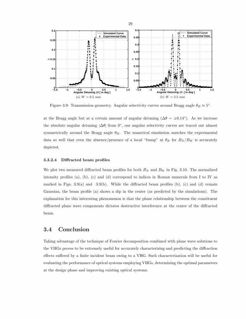
29

−1.5 −1 −0.5 0 0.5 1 1.50

0.05

0.1

0.15

0.2

0.25

0.3

Angular Detuning ∆θ [ in deg ]

η

Simulated CurveExperimental Data

I

II

−1.5 −1 −0.5 0 0.5 1 1.50

0.05

0.1

0.15

0.2

0.25

0.3

0.35

0.4

Angular Detuning ∆θ [ in deg ]

η

Simulated CurveExperimental Data

III

IV

(a) W = 0.5 mm (b) W = 2.5 mm

Figure 3.9: Transmission geometry. Angular selectivity curves around Bragg angle θB ≈ 5◦.

at the Bragg angle but at a certain amount of angular detuning (∆θ ∼ ±0.14◦). As we increase

the absolute angular detuning |∆θ| from 0◦, our angular selectivity curves are traced out almost

symmetrically around the Bragg angle θB. The numerical simulation matches the experimental

data so well that even the absence/presence of a local “bump” at θB for BN/BW is accurately

depicted.

3.3.2.4 Diffracted beam profiles

We plot two measured diffracted beam profiles for both BN and BW in Fig. 3.10. The normalized

intensity profiles (a), (b), (c) and (d) correspond to indices in Roman numerals from I to IV as

marked in Figs. 3.9(a) and 3.9(b). While the diffracted beam profiles (b), (c) and (d) remain

Gaussian, the beam profile (a) shows a dip in the center (as predicted by the simulations). The

explanation for this interesting phenomenon is that the phase relationship between the constituent

diffracted plane wave components dictates destructive interference at the center of the diffracted

beam.

3.4 Conclusion

Taking advantage of the technique of Fourier decomposition combined with plane wave solutions to

the VHGs proves to be extremely useful for accurately characterizing and predicting the diffraction

effects suffered by a finite incident beam owing to a VHG. Such characterization will be useful for

evaluating the performance of optical systems employing VHGs, determining the optimal parameters

at the design phase and improving existing optical systems.

30

0 0.5 1 1.5 2 2.5

0

0.2

0.4

0.6

0.8

1

x [ in mm ]0 0.5 1 1.5 2 2.5

0

0.2

0.4

0.6

0.8

1

x [ in mm ]

0 2 4 60

0.2

0.4

0.6

0.8

1

x [ in mm ]

Nor

mal

ized

Inte

nsity

Pro

file

0 2 4 60

0.2

0.4

0.6

0.8

1

x [ in mm ]

(a) BN (b) B

N

(c) BW

(d) BW

∆θ = 0o

∆θ = 0o

∆θ = 0.13o

∆θ = 0.13o

Figure 3.10: Normalized diffracted intensity beam profiles in the transmission geometry aroundBragg angle θB ≈ 5◦; ∆θ = θ − θB. All beam profiles are measured 50 mm from the output face.The circles represent experimental measurements and the dashed lines are the numerical simulations.

31

Bibliography

[1] H. Kogelnik. Coupled wave theory for thick hologram gratings. Bell System Technical Journal,

48(9):2909–2947, November 1969.

[2] J. W. Goodman. Fourier Optics. The McGraw-Hill Companies, Inc., Singapore, 1996.

[3] D. Psaltis, D. Brady, X. G. Xu, and S. Lin. Holography in articficial neural networks. Nature,

343:325–330, January 1990.

[4] M. Levene, G. J. Steckman, and D. Psaltis. Method for controlling the shift invariance of optical

correlators. Applied Optics, 38:394–398, January 1999.

[5] D. Gabor. Associative holographic memories. IBM Journal of Research and Development,

13(2):156, 1969.

[6] D. Psaltis and F. Mok. Holographic memories. Scientific America, 273:70–76, November 1995.

[7] G. A. Rakuljic and V. Leyva. Volume holographic narrow-band optical filter. Optics Letters,

18:459–461, March 1993.

[8] S. Breer and K. Buse. Wavelength demultiplexing with volume phase holograms in photore-

fractive lithium niobate. Applied Physics B, 66:339–345, March 1998.

[9] P. Yeh. Optical Waves in Layered Media. John Wiley & Sons, New York, 1991.

[10] V. Polo, B. Vidal, J. L. Corral, and J. Marti. Novel tunable photonic microwave filter based on

laser arrays and N×N AWG-based delay lines. IEEE Photonics Technology Letters, 15:584–586,

April 2003.

[11] S. Y. Li, N. Q. Ngo, S. C. Tjin, P. Shum, and J. Zhang. Thermally tunable narrow-bandpass

filter based on a linearly chirped fiber Bragg grating. Optics Letters, 29:29–31, January 2004.

[12] G. A. Ball and W. W. Morey. Compression-tuned single-frequency Bragg grating fiber laser.

Optics Letters, 19:1979–1981, December 1994.

[13] H. T. Hsieh, G. Panotopoulos, M. Liger, Y. C. Tai, and D. Psaltis. Athermal holographic filters.

IEEE Photonics Technology Letters, 16:177–179, January 2004.

32

Chapter 4

Athermal holographic filters

4.1 Introduction

Holographic filters[1] have been widely used for wavelength division multiplexing (WDM) filtering

applications[2, 3]. Temperature dependence is a critical concern for telecommunications. In thin

film filter technology, by proper selection of materials, we are able to combat the thermal drift of

Bragg wavelengths[4]. Athermal filter designs were also reported for arrayed-waveguide gratings

(AWGs)[5] and fiber Bragg gratings (FBGs)[6]. However, such flexibility is not available in bulk

holographic filters. In this chapter a feasible system solution for athermalizing holographic filters

will be proposed and experimentally shown to compensate for the effects of temperature changes.

4.2 Theory

A grating holographically imprinted inside a recording material can be operated as a WDM filter in

the reflection geometry, as shown in Fig. 4.1. The wavelength satisfying the grating equation

λB = 2n(T0)Λ(T0) cos θB (4.1)

B’

c-axis

recrec

B

Figure 4.1: Recording a holographic grating inside a LiNbO3 crystal at λrec= 488 nm in the trans-mission geometry and then operating it as a WDM filter in the reflection geometry.

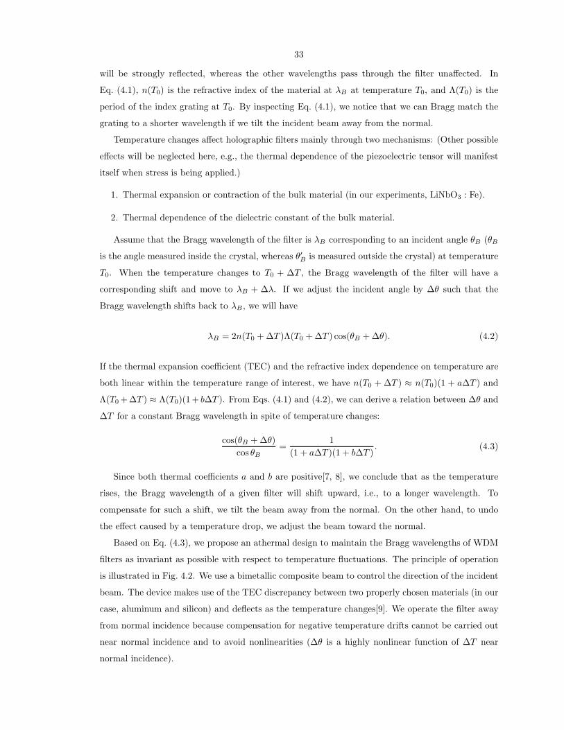
33

will be strongly reflected, whereas the other wavelengths pass through the filter unaffected. In

Eq. (4.1), n(T0) is the refractive index of the material at λB at temperature T0, and Λ(T0) is the

period of the index grating at T0. By inspecting Eq. (4.1), we notice that we can Bragg match the

grating to a shorter wavelength if we tilt the incident beam away from the normal.

Temperature changes affect holographic filters mainly through two mechanisms: (Other possible

effects will be neglected here, e.g., the thermal dependence of the piezoelectric tensor will manifest

itself when stress is being applied.)

1. Thermal expansion or contraction of the bulk material (in our experiments, LiNbO3 : Fe).

2. Thermal dependence of the dielectric constant of the bulk material.

Assume that the Bragg wavelength of the filter is λB corresponding to an incident angle θB (θB

is the angle measured inside the crystal, whereas θ′B is measured outside the crystal) at temperature

T0. When the temperature changes to T0 + ∆T , the Bragg wavelength of the filter will have a

corresponding shift and move to λB + ∆λ. If we adjust the incident angle by ∆θ such that the

Bragg wavelength shifts back to λB, we will have

λB = 2n(T0 + ∆T )Λ(T0 + ∆T ) cos(θB + ∆θ). (4.2)

If the thermal expansion coefficient (TEC) and the refractive index dependence on temperature are

both linear within the temperature range of interest, we have n(T0 + ∆T ) ≈ n(T0)(1 + a∆T ) and

Λ(T0 +∆T ) ≈ Λ(T0)(1+ b∆T ). From Eqs. (4.1) and (4.2), we can derive a relation between ∆θ and

∆T for a constant Bragg wavelength in spite of temperature changes:

cos(θB + ∆θ)

cos θB=

1

(1 + a∆T )(1 + b∆T ). (4.3)

Since both thermal coefficients a and b are positive[7, 8], we conclude that as the temperature

rises, the Bragg wavelength of a given filter will shift upward, i.e., to a longer wavelength. To

compensate for such a shift, we tilt the beam away from the normal. On the other hand, to undo

the effect caused by a temperature drop, we adjust the beam toward the normal.

Based on Eq. (4.3), we propose an athermal design to maintain the Bragg wavelengths of WDM

filters as invariant as possible with respect to temperature fluctuations. The principle of operation

is illustrated in Fig. 4.2. We use a bimetallic composite beam to control the direction of the incident

beam. The device makes use of the TEC discrepancy between two properly chosen materials (in our

case, aluminum and silicon) and deflects as the temperature changes[9]. We operate the filter away

from normal incidence because compensation for negative temperature drifts cannot be carried out

near normal incidence and to avoid nonlinearities (∆θ is a highly nonlinear function of ∆T near

normal incidence).

34

B

Al-Si Mirror

B

Figure 4.2: The athermal design of a holographic filter utilizing an Al-Si composite beam microac-tuator whose tip deflects as the temperature changes.

4.3 Experiment and results

1556 1556.3 1556.6 1556.9 1557.2 1557.5−15

−12

−9

−6

−3

0

λ (nm)

Tra

nsm

ittan

ce (

dB)

21.79oC45.68oC58.46oC

1554.8 1555 1555.2 1555.4 1555.6 1555.8 1556−7

−6

−5

−4

−3

−2

−1

0

λ [ in nm ]

Tra

nsm

ittan

ce [

in d

B ]

21.56oC40.96oC60.13oC

(a) (b)

Figure 4.3: Filter response measured in the through channel at θ′B = 5◦ for three different temper-atures (a) without and (b) with the compensating MEMS mirror.

In our experiments, holographic filters are recorded in an iron-doped lithium niobate (LiNbO3 : Fe,

0.05 wt. % Fe2O3) crystal by interfering two coherent continuous wave (cw) laser beams inside the

crystal, as shown in Fig. 4.1. The crystal sample dimensions are 2.0 cm × 1.0 cm × 0.3 cm with

its c-axis running parallel to the longest edge, and the concentration of Fe2+ is 1.28 × 1024 m−3.

A stabilization system has been incorporated into the recording setup in order to prevent the in-

terference pattern from drifting. By properly choosing the angle 2θ between the recording beams

we are able to control the Bragg wavelength of the grating operated in the reflection geometry.

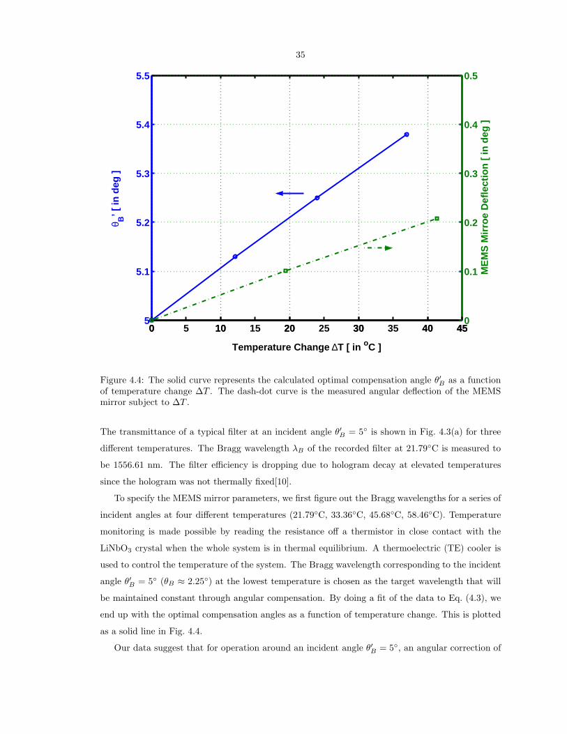
35

0 5 10 15 20 25 30 35 40 455

5.1

5.2

5.3

5.4

5.5

Temperature Change ∆T [ in oC ]

θ B’ [

in d

eg ]

0 10 20 30 40 450

0.1

0.2

0.3

0.4

0.5

ME

MS

Mirr

oe D

efle

ctio

n [ i

n de

g ]

Figure 4.4: The solid curve represents the calculated optimal compensation angle θ′B as a functionof temperature change ∆T . The dash-dot curve is the measured angular deflection of the MEMSmirror subject to ∆T .

The transmittance of a typical filter at an incident angle θ′B = 5◦ is shown in Fig. 4.3(a) for three

different temperatures. The Bragg wavelength λB of the recorded filter at 21.79◦C is measured to

be 1556.61 nm. The filter efficiency is dropping due to hologram decay at elevated temperatures

since the hologram was not thermally fixed[10].

To specify the MEMS mirror parameters, we first figure out the Bragg wavelengths for a series of

incident angles at four different temperatures (21.79◦C, 33.36◦C, 45.68◦C, 58.46◦C). Temperature

monitoring is made possible by reading the resistance off a thermistor in close contact with the

LiNbO3 crystal when the whole system is in thermal equilibrium. A thermoelectric (TE) cooler is

used to control the temperature of the system. The Bragg wavelength corresponding to the incident

angle θ′B = 5◦ (θB ≈ 2.25◦) at the lowest temperature is chosen as the target wavelength that will

be maintained constant through angular compensation. By doing a fit of the data to Eq. (4.3), we

end up with the optimal compensation angles as a function of temperature change. This is plotted

as a solid line in Fig. 4.4.

Our data suggest that for operation around an incident angle θ′B = 5◦, an angular correction of

36

1.18◦ will be required for a temperature change of 100◦C. The aluminum-silicon composite beam

was designed to deflect about 0.59◦ for a temperature change of 100◦C.

Laser

MEMS

Mirror

TE

Coolers

B’

Figure 4.5: Experimental setup combining the thermally driven MEMS mirror with the recordedholographic filter to realize the athermal filter design. A picture of the MEMS mirror is also shown.

A photograph of the MEMS mirror is shown in Fig. 4.5. It is composed of two parts: a mirror part

(surface dimensions 1.0 mm × 3.0mm, 50 nm of gold deposited on 0.45 mm silicon gives a reflectance

of 85% at 1550 nm) and a beam (surface dimensions 2.0 mm × 0.5 mm, 500 nm aluminum deposited

on 0.025 mm silicon), which deflects as the temperature varies. The measured deflection angle of

the mirror as a function of temperature is also plotted in Fig. 4.4.

We mount the holographic filter and the MEMS mirror on two separate TE coolers as depicted

in Fig. 4.5. Two identical thermistors are used to monitor the temperatures of the filter and the

mirror. The output from a tunable laser is reflected off the mirror toward the filter at an (outside)

incident angle of 5 degrees. At this point both the filter and the mirror are at room temperature.

The filter response is measured, and the Bragg wavelength is determined. Then the TE coolers are

turned on, and the temperatures of both are raised. The readings of the two thermistors are kept

the same throughout the measurements of filter response. The filter shapes at θ′B = 5◦ for three

different temperatures are plotted in Fig. 4.3(b). Compared with Fig. 4.3(a), the drift of the Bragg

wavelength is indeed compensated for by the deflection of the mirror. The compensation can be

done easily in practice because the response time of the MEMS mirror is much shorter than that of

the bulkier LiNbO3 crystal.

In Fig. 4.6 we plot the Bragg wavelengths measured with the athermal design for three different

incident angles. The dashed lines indicate the drifts of Bragg wavelengths due to the raised temper-

ature in the absence of mirror compensation. We can see that for θ′B = 5◦, the Bragg wavelength

remains constant between 21◦C and 60◦C, which corroborates the plausibility of our athermal design.

37

20 25 30 35 40 45 50 55 60 651554.8

1555

1555.2

1555.4

1555.6

1555.8

1556

1556.2

Temperature [ in oC ]

λ B [

in n

m ]

θB

’=5o

θB

’=4o

θB

’=6o

Figure 4.6: The Bragg wavelengths measured with the athermal design for three different incidentangles versus temperature.

Without the athermal mechanism, the Bragg wavelength would drift about 0.16 nm (20 GHz) from

21◦C to 60◦C. The Bragg wavelengths for θ′B = 4◦ are seen to increase with the rising temperature

despite the counteracting MEMS operation although they do not increase quite as much as when

there is no compensation mechanism; on the other hand, the Bragg wavelengths for θ′B = 6◦ are

decreasing with the rising temperature obviously because they are overcompensated by the MEMS

mirror deflection. The athermal WDM filter design employing the MEMS mirror keeps the Bragg

wavelength constant; however, to couple the reflected or transmitted beam back into a fiber, another

counteracting MEMS mirror must be used to undo the beam walk-off.

Since many thermally actuated MEMS devices consist of materials that possess different me-

chanical properties, they can suffer from hysteresis. The Bragg wavelength of the athermal filter

system undergoes a 0.09 nm (11.25 GHz) decrease after we cool it back down to room temperature.

A possible solution to this problem is to anneal the MEMS device at an elevated temperature (about

300◦C) before use. The drift in the Bragg wavelength due to hysteresis was experimentally shown

to reduce to 0.01 nm (1.25 GHz) after annealing.

38

4.4 Conclusions

We have shown that the temperature dependence of the Bragg wavelength of a holographic filter can

be compensated by incorporating a passive, thermally actuated MEMS mirror into the system. The

packaging should be such that the mirror and the filter thermally track each other. To improve the

performance of the athermal filter design, its vital to gain a deeper understanding of the evolution of

filter shapes away from normal incidence. Other topics such as beam walk-off, polarization dependent

loss (PDL) and the elimination of mirror hysteresis are also important considerations in practical

applications.

39

Bibliography

[1] G. A. Rakuljic and V. Leyva. Volume holographic narrow-band optical filter. Optics Letters,

18:459–461, March 1993.

[2] S. Breer and K. Buse. Wavelength demultiplexing with volume phase holograms in photore-

fractive lithium niobate. Applied Physics B, 66:339–345, March 1998.

[3] D. Psaltis. Coherent optical information systems. Science, 298:1359–1363, November 2002.

[4] H. Takashashi. Temperature stability of thin-film narrow-bandpass filters produced by ion-

assisted deposition. Applied Optics, 34:667–675, February 1995.

[5] N. Keil, H. H. Yao, and C. Zawadzki. Athermal polarization-independent array-waveguide

grating (AWG) multiplexer using an all-polymer approach. Applied Physics B, 73:619–622,

November 2001.

[6] Y. L. Lo and C. P. Kuo. Packaging a fiber Bragg grating without preloading in a simple athermal

bimaterial device. IEEE Transactions on Advanced Packaging, 25:50–53, February 2002.

[7] R. T. Smith and F. S. Welsh. Temperature dependence of elastic, piezoelectric, and dielectric

constants of lithium tantalite and lithium niobate. Journal of Applied Optics, 42:2219–2230,

May 1971.

[8] U. Schlarb and K. Betzler. Refractive indices of lithium niobate as a function of temperature,

wavelength and compositions-a generalized fit. Physical Review B, 48:15613–15620, December

1993.

[9] W. H. Chu, M. Mehregany, and R. L. Mullen. Analysis of tip deflection and force of a bimetalic

cantilever microactuator. Journal of Micromechanics and Microengineering, 343:4–7, February

1993.

[10] D. L. Staebler and J. J. Amodei. Thermally fixed holograms in LiNbO3. Ferroelectrics, 343:107–

113, 1972.

40

Chapter 5

Holographic filters in the 90 degree

geometry

Holograms in the 90 degree geometry have been theoretically treated before for the Bragg-matched

case, but little has been done experimentally to corroborate the analytical results. In this chapter,

we adopt coupled-mode equations to analyze such holograms in the presence of wavelength detuning.

Then we numerically simulate the field distribution and diffraction efficiency for both the Bragg-

matched and Bragg-mismatch cases, taking advantage of the characteristic spatial causality inherent

in this geometry. Experimental results of beam profiles and filtering properties will also be presented

and compared with the theoretical predictions.

5.1 Introduction

Holography has found widespread applications in modern optics. High-density data storage has

been demonstrated in transmission, 90 degree and reflection geometry holography with numerous

multiplexing schemes[1]. Over the last couple of decades, holography has also proved itself to be

a promising candidate for WDM filters, mainly in the reflection geometry[2, 3]. However, the

beam profiles and filtering properties of holograms in the 90 degree geometry remain relatively

unexplored[4]. In this chapter, we will present some experimental results for the 90-degree-geometry

holography as well as numerical simulations based on coupled mode analysis.

This chapter is organized as follows. In section 2 we define a hologram of interest in the 90 degree

geometry and summarize theoretical predictions by Kenan[5] in the Bragg-matched condition. In

section 3 we take a step farther and derive the coupled mode equations in the presence of wavelength

mismatch, therefore laying the foundation for numerical simulation, the results of which will then

be subsequently presented in section 4. Section 5 will be devoted to showing some of the relevant

experimental results and comparing them with the theoretical and numerical analyses. In section

6, we draw our conclusion as to the possible applications of the 90-degree-geometry holograms in

41

k2’

Q(x,y)

k1’ P(x,y)

W1

y (output face)

W2

x

n(x,y)

z

Figure 5.1: A schematic graph of a grating in the 90 degree geometry.

WDM filter design.

5.2 Beam propagation in the 90 degree geometry holograms

A grating in the 90 degree geometry is shown in Fig. 5.1. It is formed by interfering two coherent

beams inside a piece of photorefractive material (LiNbO3, for example) whose refractive index is

therefore periodically modulated. Assume that the two beams used to generate the grating are

polarized perpendicular to the xy plane and have the following field profiles:

E1(r) = E10 exp(−jk1 · r), (5.1)

E2(r) = E20 exp(−jk2 · r), (5.2)

where E10 and E20 are the amplitudes of the plane wavefronts and k1 = (k/2,−k/2, kz), k2 =

(−k/2, k/2, kz). Furthermore, k and kz are related to the recording wavelength λrec by the following

equation:

|k1| = |k2| =2πnrec

λrec=

√

k2

2+ k2

z , (5.3)

where nrec stands for the bulk refractive index of the medium at the recording wavelength λrec. The

two beams interfere with each other throughout the crystal and create a grating of constant index

42

modulation ∆n on each plane defined by a constant z:

n(x, y) = n0 + ∆n cos k(x − y). (5.4)

The bulk index of the medium n0 and the index modulation ∆n are constants whose values will be

determined by the readout wavelength λ′0. We will assume ∆n � n0, as is usually the case. Now

say we have an incident beam (assumed to be polarized along the z-axis) with a beam profile Q(x, y)

and wave vector k′2 = k′ax (here ax is the unit vector along the x-axis and k′ = 2πn0λ

′0 = k′

0n0,

where λ′0 is the incident wavelength in vacuum) as in Fig. 5.1. If k′ ≈ k, the total field distribution

inside the grating region that thus ensues can be cast into the form:

E(x, y) = P (x, y) exp(−jk′1 · r) + Q(x, y) exp(−jk′

2 · r), (5.5)

conceivably, k′1 = k′ay ≈ kay and P (x, y) is the diffracted field distribution. Kenan has detailed the

Bragg-matched case (i.e., k′ = k = 2πn0/λ0, where λ0 is the Bragg wavelength) in his paper[5], and

we repeat his analytical results below:

Q(x, y) = Q0J0(2κ√

xy) − jP0

√

x

yJ1(2κ

√xy),

P (x, y) = P0J0(2κ√

xy) − jQ0

√

y

xJ1(2κ

√xy), (5.6)

where κ = π∆n/λ0. We therefore realize that for the Bragg-matched case, the incident and diffracted

beam profiles within the uniform grating region can be described analytically by the zeroth- and

first-order Bessel functions of the first kind. What Kenan did not consider in his paper, however,

are the cases where we have a Bragg-mismatch component either due to a wavelength detuning or

an angular deviation.

In the 90 degree geometry, the diffracted beam is nonuniform for a constant refractive index

modulation and a uniform incident beam. As a result, the diffraction efficiency is defined as the

total power ratio of the incident and diffracted beams[6]. We have from Eq. (5.6):

η = 1 − J20 (2κ

√

W1W2) − J21 (2κ

√

W1W2). (5.7)

It is worth pointing out that the diffraction efficiency η is a non-decreasing function that has zero

derivatives only at zeros of the Bessel function of the first kind, order 1.

43

y

x

Figure 5.2: The grating region has been divided into tiny rectangular regions to facilitate numericalsimulation.

5.3 Wavelength selectivity

Now we consider the case where the incident wavelength λ′0 is different from the Bragg wavelength

λ0 assuming the absence of angular detuning for simplicity, i.e., k′1//ay, k′

2//ax and k′1 = k′

2 6= k.

We also assume that the difference between λ0 and λ′0 is small enough that the material dispersion

is negligible. Substituting Eq. (5.5) into the Helmholtz equation we get:

[∂2

∂x2P +

∂2

∂y2P − 2jk′ ∂

∂yP − k′2P ] exp(−jk′y) + [

∂2

∂x2Q +

∂2

∂y2Q − 2jk′ ∂

∂xQ − k′2Q] exp(−jk′x)

+k′20 [n2

0 + 2n0∆n cos k(x − y)][P exp(−jk′y) + Q exp(−jk′x)] = 0.(5.8)

We have neglected the term involving ∆n2 because it is minute compared with terms associated with

n20 and n0∆n; we further adopt the parabolic approximation that entitles us to ignore the second

order partial differential terms. After some straightforward algebraic manipulations, we end up with

∂Q

∂x+ jκ′P exp [j(k′ − k)(x − y)] = 0,

∂P

∂y+ jκ′Q exp [j(k − k′)(x − y)] = 0, (5.9)

where κ′ = π∆n/λ′0. To get back the Bragg-matched case, we can simply set k′ = k. Although the

analytical solution to Eq. (5.9) is not available, we can numerically simulate the Bragg-mismatch

case and still get the desired beam profiles and diffraction efficiency, which will be presented shortly.

44

P

Q

x

y

11

M

N

(a) (b) (c)

(d) (e)

Figure 5.3: Working principle of the numerical simulation. The inherent causality of gratings in the90 degree geometry facilitates the algorithm.

5.4 Numerical simulations

In this section we shall simulate for the wavelength detuning case. We start by discretizing Eq. (5.9):

Q(x+δx,y)−Q(x,y)δx

+ jκ′P (x, y) exp [j(k′ − k)(x − y)] = 0,

P (x,y+δy)−P (x,y)δx

+ jκ′Q(x, y) exp [−j(k′ − k)(x − y)] = 0,

which can be further simplified to

Q(x + δx, y) = Q(x, y) − jδxκ′P (x, y) exp [j(k′ − k)(x − y)] ,

P (x, y + δy) = P (x, y) − jδyκ′Q(x, y) exp [−j(k′ − k)(x − y)] . (5.10)

Eq. (5.10) implies that if we divide the grating region into tiny rectangular cells with dimension

δx × δy as shown in Fig. 5.2 and happen to know the values of both P (x, y) and Q(x, y) in a certain

cell, we can calculate both the value of P (x, y + δy) in the next cell along the y-direction and the

value of Q(x + δx, y) in the next cell along the x-direction. In our simulations, the incident beam is

uniform over the input face defined by x = 0, 0 ≤ y ≤ W2, and no diffracted beam is present at the

face defined by y = 0, 0 ≤ x ≤ W1; therefore we have the following boundary conditions:

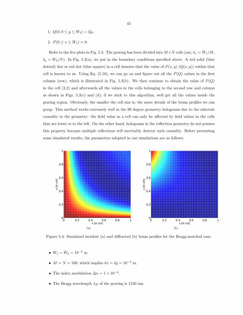
45

1. Q(0, 0 ≤ y ≤ W2) = Q0.

2. P (0 ≤ x ≤ W1) = 0.

Refer to the five plots in Fig. 5.3. The grating has been divided into M×N cells (say, δx = W1/M ,

δy = W2/N). In Fig. 5.3(a), we put in the boundary conditions specified above. A red solid (blue

dotted) line or red dot (blue square) in a cell denotes that the value of P (x, y) (Q(x, y)) within that

cell is known to us. Using Eq. (5.10), we can go on and figure out all the P (Q) values in the first

column (row), which is illustrated in Fig. 5.3(b). We then continue to obtain the value of P (Q)

in the cell (2,2) and afterwards all the values in the cells belonging to the second row and column

as shown in Figs. 5.3(c) and (d); if we stick to this algorithm, well get all the values inside the

grating region. Obviously, the smaller the cell size is, the more details of the beam profiles we can

grasp. This method works extremely well in the 90 degree geometry holograms due to the inherent

causality in the geometry: the field value in a cell can only be affected by field values in the cells

that are lower or to the left. On the other hand, holograms in the reflection geometry do not possess

this property because multiple reflections will inevitably destroy such causality. Before presenting

some simulated results, the parameters adopted in our simulations are as follows:

0 0.2 0.4 0.6 0.8 10

0.2

0.4

0.6

0.8

1

x (in cm)

y (in

cm

)

0 0.2 0.4 0.6 0.8 10

0.2

0.4

0.6

0.8

1

x (in cm)

y (in

cm

)

(a) (b)

Figure 5.4: Simulated incident (a) and diffracted (b) beam profiles for the Bragg-matched case.

• W1 = W2 = 10−2 m.

• M = N = 100, which implies δx = δy = 10−4 m.

• The index modulation ∆n = 1 × 10−4.

• The Bragg wavelength λB of the grating is 1550 nm.

46

0 0.2 0.4 0.6 0.8 10

0.2

0.4

0.6

0.8

1

x (in cm)

y (in

cm

)

0 0.2 0.4 0.6 0.8 10

0.2

0.4

0.6

0.8

1

x (in cm)

y (in

cm

)

(a) (b)

Figure 5.5: Simulated incident (a) and diffracted (b) beam profiles for the Bragg mismatch case.

We numerically simulate the beam profiles in Fig. 5.1 using Eq. (5.10) for the Bragg-matched

case where ∆n is constant and the incident beam is uniform over the input face. The beam profiles

at Bragg wavelength are shown in Fig. 5.4. We can see that the field distribution of the incident

beam is symmetric with respect to the line x = y, which is consistent with the analytical prediction;

furthermore, the grating directs most of the incident beam towards the output face, and the diffracted

beam has a tendency to concentrate as close to the input face as possible. The stronger the grating

is, the more obvious the phenomenon will be. A uniform incident beam will invariably result in a

nonuniform diffracted beam profile. In light of Eq. (5.6), the diffracted beam profile at the output

face can be described by the Bessel function of the first kind. The diffracted beam intensity profile

at the crystal output face obtained from the numerical simulation is indistinguishable from the

analytical expression.

Being confident that our numerical method does produce results confirmed by the analytical

solution, we go on and simulate the diffracted beam profile in the Bragg-mismatch case for a uniform

incident beam, the result of which is plotted in Fig. 5.5 for a wavelength mismatch ∆λ = λ0−λ′0 = 0.1

nm, other parameters are the same as those adopted in Fig. 5.4. We notice that the beam deflection

ability is weaker for this (Bragg-mismatch) case, and less incident light manages to make its way to

the output face.

Plotted for comparison in Fig. 5.6 is the normalized diffracted beam intensity along the output

face; they have been normalized to the peak diffracted intensity of the Bragg-matched case.

To visualize the magnitude response of a given grating, we run the program for different wave-

lengths of interest and then calculate the diffraction efficiency for each wavelength. For wavelengths

other than the Bragg wavelength a mismatch phase factor has to be included in the simulation. To

47

0 0.2 0.4 0.6 0.8 10

0.1

0.2

0.3

0.4

0.5

0.6

0.7

0.8

0.9

1

x (in cm)

Nor

mal

ized

Diff

ract

ed B

eam

Inte

nsity

Pro

file

Simulated Profile [Bragg−matched]Analytical Solution [Bragg−matched]Simulated Profile [ ∆λ=0.1 nm]

Figure 5.6: Normalized diffracted beam intensity profiles for the Bragg-matched (traced out bycrosses) and Bragg-mismatch cases (denoted by squares). The solid curve is plotted according tothe analytical solution of the Bragg-matched case Eq. (5.6), which fits excellently with our numericalprediction.

(in nm)

P

1549 1549.5 1550 1550.5 15510

0.2

0.4

0.6

0.8

1

n=5 10-4

n=2 10-4

n=1 10-4

n=5 10-5

Figure 5.7: Simulated magnitude response of 90 degree geometry gratings for various index modu-lation ∆n.

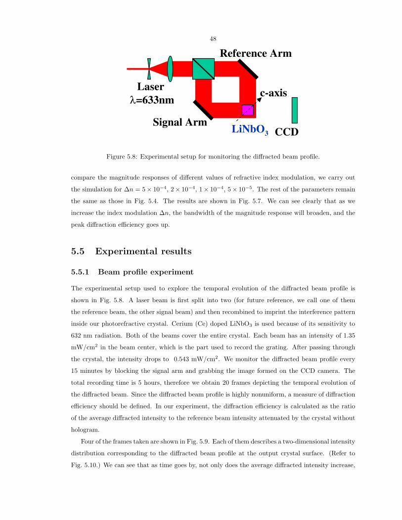
48

c-axis

LiNbO3

Reference Arm

Signal ArmCCD

Laser

=633nm

Figure 5.8: Experimental setup for monitoring the diffracted beam profile.

compare the magnitude responses of different values of refractive index modulation, we carry out

the simulation for ∆n = 5× 10−4, 2× 10−4, 1× 10−4, 5 × 10−5. The rest of the parameters remain

the same as those in Fig. 5.4. The results are shown in Fig. 5.7. We can see clearly that as we

increase the index modulation ∆n, the bandwidth of the magnitude response will broaden, and the

peak diffraction efficiency goes up.

5.5 Experimental results

5.5.1 Beam profile experiment

The experimental setup used to explore the temporal evolution of the diffracted beam profile is

shown in Fig. 5.8. A laser beam is first split into two (for future reference, we call one of them

the reference beam, the other signal beam) and then recombined to imprint the interference pattern

inside our photorefractive crystal. Cerium (Ce) doped LiNbO3 is used because of its sensitivity to

632 nm radiation. Both of the beams cover the entire crystal. Each beam has an intensity of 1.35

mW/cm2 in the beam center, which is the part used to record the grating. After passing through

the crystal, the intensity drops to 0.543 mW/cm2. We monitor the diffracted beam profile every

15 minutes by blocking the signal arm and grabbing the image formed on the CCD camera. The

total recording time is 5 hours, therefore we obtain 20 frames depicting the temporal evolution of

the diffracted beam. Since the diffracted beam profile is highly nonuniform, a measure of diffraction

efficiency should be defined. In our experiment, the diffraction efficiency is calculated as the ratio

of the average diffracted intensity to the reference beam intensity attenuated by the crystal without

hologram.

Four of the frames taken are shown in Fig. 5.9. Each of them describes a two-dimensional intensity

distribution corresponding to the diffracted beam profile at the output crystal surface. (Refer to

Fig. 5.10.) We can see that as time goes by, not only does the average diffracted intensity increase,

49

Figure 5.9: Temporal evolution of the diffracted beam profile formed on the CCD camera.

x

Reference

beam

Input

face

Output

face

Figure 5.10: The variable x is used in Eq. (5.11) for the calculation of diffracted beam profiles.

but more light is also squeezed toward the input surface. These phenomena can be explained if

we write down the analytical solution of the diffracted beam intensity profile at the output surface

according to Eq. (5.6):

IP (x) = IQ0WJ2

1 (2κ√

Wx)

x, (5.11)

where κ = π∆n/λ′0 is the coupling constant and the variable x represents the distance along the

output face measured from the input plane, as shown in Fig. 5.10. W is the dimension of the crystal,

which is 1 cm in our case. To illustrate the squeezing effect brought about by the buildup of index

modulation, we plot the theoretical IP (x)/IP (0) for three different coupling constants in Fig. 5.11.

It is obvious that as ∆n increases, the relative intensity of the diffracted beam close to the input

face will also increase.

To explain the increasing trend of overall diffraction efficiency η, we remember that the analytical

solution for the diffraction efficiency is (from Eq. (5.7), substitute W for W1 and W2):

η = 1 − J20 (2κW ) − J2

1 (2κW ). (5.12)

Eq. (5.12) is seen to be a monotonically non-decreasing function of κ (∂η/∂κ ≥ 0). Therefore, we

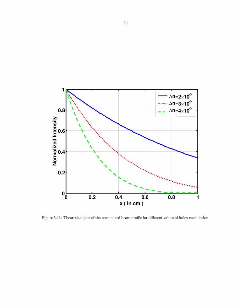
50

0 0.2 0.4 0.6 0.8 10

0.2

0.4

0.6

0.8

1

x ( in cm )

No

rma

lize

d In

ten

sit

y

n=2 10-5

=3 10-5

=4 10-5

n

n

Figure 5.11: Theoretical plot of the normalized beam profile for different values of index modulation.

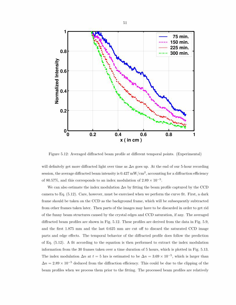
51

0 0.2 0.4 0.6 0.8 10

0.2

0.4

0.6

0.8

1

x ( in cm )

No

rma

lize

d In

ten

sit

y

75 min.150 min.225 min.300 min.

Figure 5.12: Averaged diffracted beam profile at different temporal points. (Experimental)

will definitely get more diffracted light over time as ∆n goes up. At the end of our 5-hour recording

session, the average diffracted beam intensity is 0.427 mW/cm2, accounting for a diffraction efficiency

of 80.57%, and this corresponds to an index modulation of 2.89 × 10−5.

We can also estimate the index modulation ∆n by fitting the beam profile captured by the CCD

camera to Eq. (5.12). Care, however, must be exercised when we perform the curve fit. First, a dark

frame should be taken on the CCD as the background frame, which will be subsequently subtracted

from other frames taken later. Then parts of the images may have to be discarded in order to get rid

of the funny beam structures caused by the crystal edges and CCD saturation, if any. The averaged

diffracted beam profiles are shown in Fig. 5.12. These profiles are derived from the data in Fig. 5.9,

and the first 1.875 mm and the last 0.625 mm are cut off to discard the saturated CCD image

parts and edge effects. The temporal behavior of the diffracted profile does follow the prediction

of Eq. (5.12). A fit according to the equation is then performed to extract the index modulation

information from the 30 frames taken over a time duration of 5 hours, which is plotted in Fig. 5.13.

The index modulation ∆n at t = 5 hrs is estimated to be ∆n = 3.69 × 10−5, which is larger than

∆n = 2.89 × 10−5 deduced from the diffraction efficiency. This could be due to the clipping of the

beam profiles when we process them prior to the fitting. The processed beam profiles are relatively

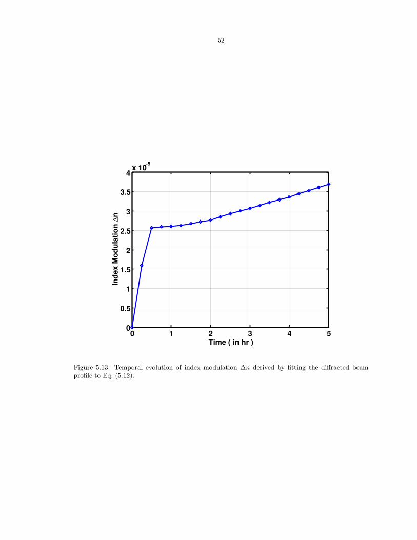
52

0 1 2 3 4 50

0.5

1

1.5

2

2.5

3

3.5

4x 10

-5

Time ( in hr )

Ind

ex

Mo

du

lati

on

n

Figure 5.13: Temporal evolution of index modulation ∆n derived by fitting the diffracted beamprofile to Eq. (5.12).

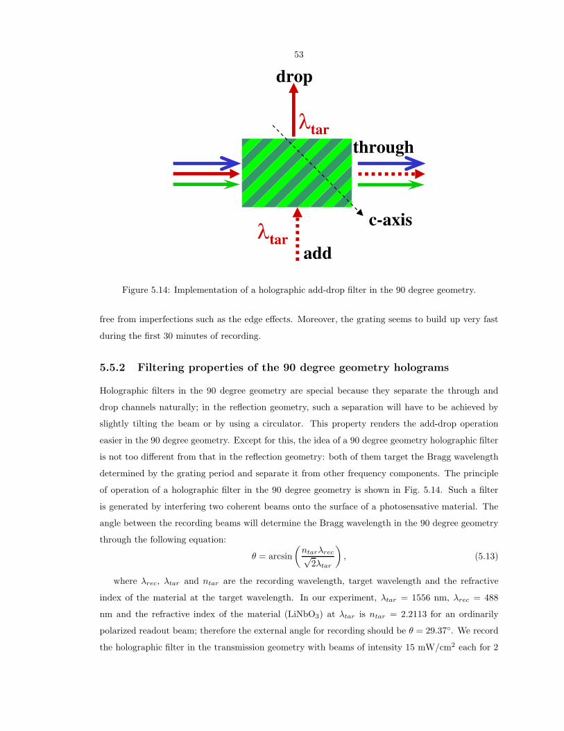
53

c-axis

drop

throughtar

addtar

Figure 5.14: Implementation of a holographic add-drop filter in the 90 degree geometry.

free from imperfections such as the edge effects. Moreover, the grating seems to build up very fast

during the first 30 minutes of recording.

5.5.2 Filtering properties of the 90 degree geometry holograms

Holographic filters in the 90 degree geometry are special because they separate the through and

drop channels naturally; in the reflection geometry, such a separation will have to be achieved by

slightly tilting the beam or by using a circulator. This property renders the add-drop operation

easier in the 90 degree geometry. Except for this, the idea of a 90 degree geometry holographic filter

is not too different from that in the reflection geometry: both of them target the Bragg wavelength

determined by the grating period and separate it from other frequency components. The principle

of operation of a holographic filter in the 90 degree geometry is shown in Fig. 5.14. Such a filter

is generated by interfering two coherent beams onto the surface of a photosensative material. The

angle between the recording beams will determine the Bragg wavelength in the 90 degree geometry

through the following equation:

θ = arcsin

(

ntarλrec√2λtar

)

, (5.13)

where λrec, λtar and ntar are the recording wavelength, target wavelength and the refractive

index of the material at the target wavelength. In our experiment, λtar = 1556 nm, λrec = 488

nm and the refractive index of the material (LiNbO3) at λtar is ntar = 2.2113 for an ordinarily

polarized readout beam; therefore the external angle for recording should be θ = 29.37◦. We record

the holographic filter in the transmission geometry with beams of intensity 15 mW/cm2 each for 2

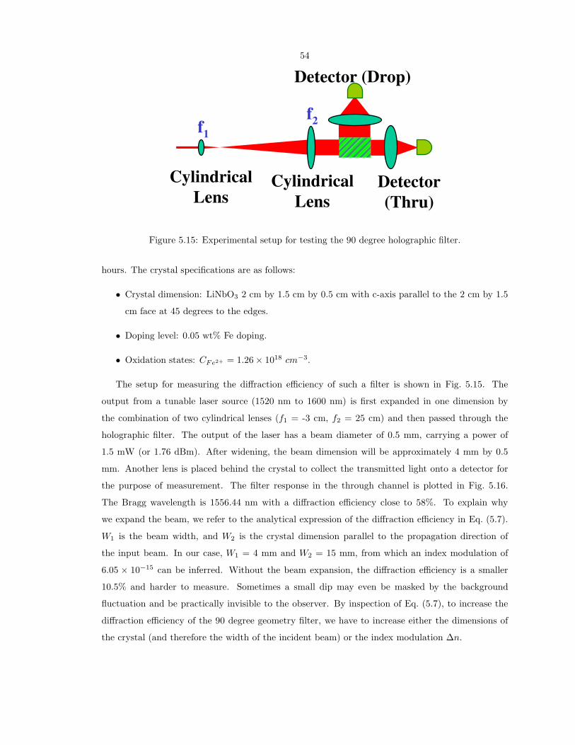
54

Cylindrical

Lens

f1

f2

Cylindrical

Lens

Detector

(Thru)

Detector (Drop)

Figure 5.15: Experimental setup for testing the 90 degree holographic filter.

hours. The crystal specifications are as follows:

• Crystal dimension: LiNbO3 2 cm by 1.5 cm by 0.5 cm with c-axis parallel to the 2 cm by 1.5

cm face at 45 degrees to the edges.

• Doping level: 0.05 wt% Fe doping.

• Oxidation states: CFe2+ = 1.26 × 1018 cm−3.

The setup for measuring the diffraction efficiency of such a filter is shown in Fig. 5.15. The

output from a tunable laser source (1520 nm to 1600 nm) is first expanded in one dimension by

the combination of two cylindrical lenses (f1 = -3 cm, f2 = 25 cm) and then passed through the

holographic filter. The output of the laser has a beam diameter of 0.5 mm, carrying a power of

1.5 mW (or 1.76 dBm). After widening, the beam dimension will be approximately 4 mm by 0.5

mm. Another lens is placed behind the crystal to collect the transmitted light onto a detector for

the purpose of measurement. The filter response in the through channel is plotted in Fig. 5.16.

The Bragg wavelength is 1556.44 nm with a diffraction efficiency close to 58%. To explain why

we expand the beam, we refer to the analytical expression of the diffraction efficiency in Eq. (5.7).

W1 is the beam width, and W2 is the crystal dimension parallel to the propagation direction of

the input beam. In our case, W1 = 4 mm and W2 = 15 mm, from which an index modulation of

6.05 × 10−15 can be inferred. Without the beam expansion, the diffraction efficiency is a smaller

10.5% and harder to measure. Sometimes a small dip may even be masked by the background

fluctuation and be practically invisible to the observer. By inspection of Eq. (5.7), to increase the

diffraction efficiency of the 90 degree geometry filter, we have to increase either the dimensions of

the crystal (and therefore the width of the incident beam) or the index modulation ∆n.

55

1555 1555.5 1556 1556.5 1557 1557.5 1558-7

-6.5

-6

-5.5

-5

-4.5

-4

-3.5

-3

-2.5

(in nm)

Th

rou

gh

Ch

an

nel

Read

ing

(in

dB

m)

Figure 5.16: Experimental filter response measured in the filter through (transmission) channel.(This corresponds to an index modulation of ∆n = 6 × 10−5.)

5.6 Conclusion

Experiments on beam profiles in the 90 degree geometry holography corroborate the theoretical

predictions and give us a clear idea of how an incident beam interacts with the grating. The

selective behavior demonstrated in the frequency response is certainly reminiscent of holographic

filters. Holographic filters in the 90 degree geometry have the advantage of naturally separating the

diffracted frequency components from the transmitted ones. Nevertheless, deliberation on the filter

geometry also reveals the fact that strong dispersion will be introduced for the diffracted wavelength

components. Such a property is generally undesirable in WDM filters, but it may be valuable in

applications regarding dispersion compensation.

56

Bibliography

[1] M. H. Yukselici, R. Ince, and A. T. Ince. Data storage characteristics of iron doped LiNbO3

under a 90 degrees geometry two-beam coupling configuration. Optics and Lasers in Engineering,

42:277–287, September 2004.

[2] G. A. Rakuljic and V. Leyva. Volume holographic narrow-band optical filter. Optics Letters,

18:459–461, March 1993.

[3] S. Breer and K. Buse. Wavelength demultiplexing with volume phase holograms in photorefrac-

tive lithium niobate. Applied Physics B, 66:339–345, March 1998.

[4] Y. Yang, A. Adibi, and D. Psaltis. Comparison of transmission and the 90-degree holographic

recording geometry. Applied Optics, 42(17):3418–3427, June 2003.

[5] R. P. Kenan. Theory of crossed-beam diffraction gratings. IEEE Journal of Quantum Electronics,

14:924–930, December 1978.

[6] L. Solymar and D. J. Cooke. Volume Holography and Volume Gratings. Academic Press, New

York, 1981.

57

Chapter 6

Femtosecond holography in Kerr

media

The femtosecond holographic pump-probe technique is useful for investigating ultrafast material

phenomena. We demonstrate, in theory and experiment, that the temporal resolution in such con-

figurations does not degrade appreciably despite increasing angular separation between the pump

pulses. Transient Kerr gratings are generated inside calcium fluoride (CaF2) crystals by two inter-

fering femtosecond (pump) pulses at 388 nm and read out by a Bragg-matched probe pulse at 776

nm. The solution to the coupled mode equations of pulse holography is well corroborated by the

experimental results, yielding a value of Kerr coefficient 4.4 × 10−7 cm2/GW for CaF2.

6.1 Introduction

Femtosecond pump-probe techniques have become a very powerful tool for investigating various

ultrafast phenomena in materials. They proved fruitful in many research areas, e.g., characteriza-

tion of carrier dynamics in semiconductors[1, 2], parametric up-conversion processes[3], femtosecond

spectroscopy[4] and nondestructive examination of materials[5], just to name a few.

In a holographic pump-probe experiment, two intense, identical pump pulses overlap temporally

and spatially in a nonlinear medium to induce (by interference) periodically modulated material

responses within the region of intersection. A probe pulse then experiences the ensuing optical

perturbations and gets diffracted when the Bragg condition is met. The diffracted probe pulse is

picked up by a detector; the detected signal as a function of the time delay between the pump and

probe pulses is then mapped out and gives information about the involved ultrafast mechanisms of

interest.

The coupled mode equations of femtosecond holography are different from those of continuous-

wave holography[6]. In this article, the coupled mode equations for pulse holography are solved in

the case of Kerr nonlinearity for an undepleted, Bragg-matched probe pulse. The nonlinear responses

58

!r !p

(a)

!r

!p

Wp

Wr

(b)

Figure 6.1: The temporal resolution in two-pulse pump-and-probe experiments is strongly affectedby the transverse pulse widths and the angle θ between the pulses involved. Optimal resolution isobtained when the pulses propagate collinearly, as in case (a); deviation from collinearity causes theresolution to deteriorate due to the transverse dimensions of the pulses, as in case (b).

of the medium are assumed to be instantaneous compared with the pulse duration[7].

In the conventional single-pump-and-single-probe experiments[8], the temporal resolution cannot

be better than the cross-correlation trace of the pulses involved. Optimal resolution is obtained

when the pulses propagate collinearly; deviation from collinearity generally causes the resolution to

deteriorate as a result of the transverse dimensions of the pulses[9, 10].

For a simple illustration, refer to Fig. 6.1. We consider two extreme cases, i.e., when the pump

and probe pulses are propagating parallel, in case (a), or perpendicular, in case (b), to each other.

For clarity, we assume that the two pulses are spatially and temporally rectangular and they have the

same group velocity v. In the figure, τ/W specifies the pulse temporal duration/transverse dimension

and subscript p/r stands for pump/probe. In case (a), the temporal resolution is approximately

τp + τr; on the other hand, in case (b) it will roughly be τp + τr +Wp+Wr

v . When propagating

collinearly, the pulse temporal durations alone determine the temporal resolution. Moving away

from collinearity, the pulse transverse dimensions start to affect temporal resolution, dominating

in the perpendicular case. The bigger Wp and Wr are, the more pronounced such an effect will

be. We will show that such a phenomenon is almost absent in the holographic pump-and-probe

configuration.

In this chapter, experiments conducted in calcium fluoride (CaF2) samples are used to verify

the theoretical prediction; the temporal resolution of the femtosecond holographic configuration is

investigated. An advantage of this configuration is that the natural separation between the diffracted

probe pulse and the pump pulses mitigates the difficulty of detection suffered by collinear pump-

and-probe experiments.

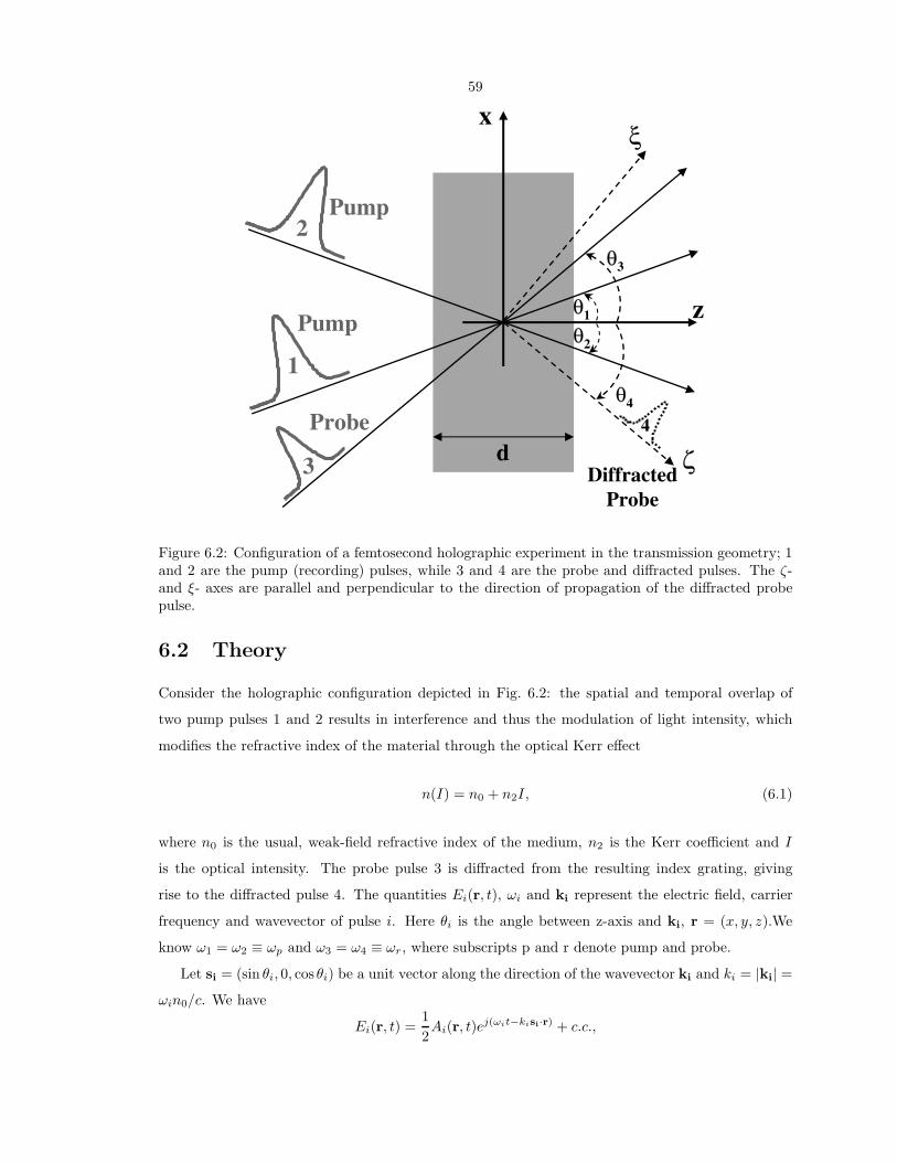
59

d

z

x

Pump

Pump

Probe

2

1

2

3

4

4

Diffracted

Probe

1

3

Figure 6.2: Configuration of a femtosecond holographic experiment in the transmission geometry; 1and 2 are the pump (recording) pulses, while 3 and 4 are the probe and diffracted pulses. The ζ-and ξ- axes are parallel and perpendicular to the direction of propagation of the diffracted probepulse.

6.2 Theory

Consider the holographic configuration depicted in Fig. 6.2: the spatial and temporal overlap of

two pump pulses 1 and 2 results in interference and thus the modulation of light intensity, which

modifies the refractive index of the material through the optical Kerr effect

n(I) = n0 + n2I, (6.1)

where n0 is the usual, weak-field refractive index of the medium, n2 is the Kerr coefficient and I

is the optical intensity. The probe pulse 3 is diffracted from the resulting index grating, giving

rise to the diffracted pulse 4. The quantities Ei(r, t), ωi and ki represent the electric field, carrier

frequency and wavevector of pulse i. Here θi is the angle between z-axis and ki, r = (x, y, z).We

know ω1 = ω2 ≡ ωp and ω3 = ω4 ≡ ωr, where subscripts p and r denote pump and probe.

Let si = (sin θi, 0, cos θi) be a unit vector along the direction of the wavevector ki and ki = |ki| =

ωin0/c. We have

Ei(r, t) =1

2Ai(r, t)e

j(ωit−kisi·r) + c.c.,

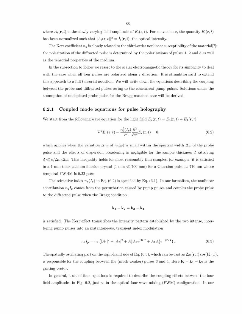
60

where Ai(r, t) is the slowly varying field amplitude of Ei(r, t). For convenience, the quantity Ei(r, t)

has been normalized such that |Ai(r, t)|2 = Ii(r, t), the optical intensity.

The Kerr coefficient n2 is closely related to the third-order nonlinear susceptibility of the material[7];

the polarization of the diffracted pulse is determined by the polarizations of pulses 1, 2 and 3 as well

as the tensorial properties of the medium.

In the subsection to follow we resort to the scalar electromagnetic theory for its simplicity to deal

with the case when all four pulses are polarized along y direction. It is straightforward to extend

this approach to a full tensorial notation. We will write down the equations describing the coupling

between the probe and diffracted pulses owing to the concurrent pump pulses. Solutions under the

assumption of undepleted probe pulse for the Bragg-matched case will be derived.

6.2.1 Coupled mode equations for pulse holography

We start from the following wave equation for the light field Er(r, t) = E3(r, t) + E4(r, t),

∇2Er(r, t) −n2

r(Ip)

c2

∂2

∂t2Er(r, t) = 0, (6.2)

which applies when the variation ∆n0 of n0(ω) is small within the spectral width ∆ω of the probe

pulse and the effects of dispersion broadening is negligible for the sample thickness d satisfying

d � c/∆n0∆ω. This inequality holds for most reasonably thin samples; for example, it is satisfied

in a 1-mm thick calcium fluoride crystal (1 mm � 700 mm) for a Gaussian pulse at 776 nm whose

temporal FWHM is 0.22 psec.

The refractive index nr(Ip) in Eq. (6.2) is specified by Eq. (6.1). In our formalism, the nonlinear

contribution n2Ip comes from the perturbation caused by pump pulses and couples the probe pulse

to the diffracted pulse when the Bragg condition

k1 − k2 = k3 − k4

is satisfied. The Kerr effect transcribes the intensity pattern established by the two intense, inter-

fering pump pulses into an instantaneous, transient index modulation

n2Ip = n2

(

|A1|2 + |A2|2 + A∗1A2e

jK·r + A1A∗2e

−jK·r)

. (6.3)

The spatially oscillating part on the right-hand side of Eq. (6.3), which can be cast as ∆n(r, t) cos(K · r),is responsible for the coupling between the (much weaker) pulses 3 and 4. Here K = k1 − k2 is the

grating vector.

In general, a set of four equations is required to describe the coupling effects between the four

field amplitudes in Fig. 6.2, just as in the optical four-wave mixing (FWM) configuration. In our

61

femtosecond holographic setting, the pump amplitudes A1 and A2 are barely affected by the probe

amplitudes A3 and A4 because pump pulses are much more intense. Moreover, it is justifiable to

neglect the coupling effects between A1 and A2 due to a weak coupling strength. As a result, we

can conveniently discard the differential equations associated with A1 and A2 and incorporate their

effects into the term ∆n(r, t).

We can write down the following coupled mode equations for pulse holography when the Bragg

condition is satisfied (vr is the group velocity of the probe pulse):

[

(s3 · ∇) +1

vr

∂

∂t

]

A3 = −jπ∆n

λrA4, (6.4a)

[

(s4 · ∇) +1

vr

∂

∂t

]

A4 = −jπ∆n

λrA3. (6.4b)

In arriving at the equations Eqs. (6.4a) and (6.4b) above, several approximations have been

adopted:

– Only the third-order material nonlinearity comes into play. The second-order nonlinearity

term is discarded for irrelevance; higher order terms are also ignored because the third order

term dominates in magnitude.

– We ignore the terms associated with (∆n)2 and keep those involving n∆n because typically

(and in our experiments) ∆n/n ≤ 10−4.

– We ignore the second order terms ∂2

∂t2 Ai compared with ωr∂∂tAi since the spectral bandwidth

∆ωi of Ai is much smaller than its carrier frequency ωr.

– The longitudinal second-order derivative (si · ∇)2Ai is ignored compared with kr(si · ∇)Ai

because the spatial bandwidth ∆ki of Ai is much smaller than its carrier kr (slowly varying

amplitude approximation). The transverse second-order derivative are also ignored thanks to

the next two conditions.

– Diffraction broadening is negligible because the Rayleigh range of the pulse is much longer

than the sample thickness.

– The self-focusing effects experienced by the intense pump pulses can be ignored when the

self-focusing distance is much larger than the sample thickness[7].

The main difference between the coupled mode equations Eqs. (6.4a) and (6.4b) for pulse hologra-

phy and those for continuous-wave (cw) holography is the presence of the time derivative to account

for the short pulse temporal duration. Furthermore, the amplitude Ai is a function of both x and z

since the pulses have finite spatial extent[11].

62

6.2.2 Solution of the diffracted pulse: undepleted incident probe

We can solve for the amplitude of the diffracted pulse A4 using only Eq. (6.4b) if we make the

assumption that the probe pulse is undepleted by the transient grating; this is equivalent to the

first Born approximation[12]. To facilitate the solution, we convert to a retarded time frame by

performing the following change of variables:

ζ = z cos θ4 + x sin θ4,

ξ = x cos θ4 − z sin θ4,

τ = t − z

vrcos θ4 −

x

vrsin θ4,

where τ is the retarded time and ζ/ξ is the longitudinal/transverse spatial coordinate of the diffracted

pulse, as shown in Fig. 6.2. Let r′ = (ξ, y, ζ); straightforward substitution leads us to a much more

simplified differential equation from Eq. (6.4b):

∂A4(r′, τ)

∂ζ= −j

π∆n(r′, τ)

λrA3(r

′, τ). (6.5)

The boundary condition A4

(

z = − d2

)

= 0 translates into A4

(

ζ = − d2 sec θ4 + ξ tan θ4

)

= 0 and leads

to the solution at z = d/2

A4(ξ, y, z = d/2, τ) =−jπ

λr

d2 sec θ4+ξ tan θ4

∫

− d2 sec θ4+ξ tan θ4

∆nA3dζ. (6.6)

The diffraction efficiency η is defined as the energy ratio between the diffracted pulse and trans-

mitted pulse.

η =

∫

∞∫

−∞

∫

|A4(ζ = d2 sec θ4 + ξ tan θ4)|2dξdydτ

∫

∞∫

−∞

∫

|A3(z = d2 )|2dxdydt

. (6.7)

The amplitudes of pump and probe pulses (i = 1, 2, 3) can be represented as Ai(r′, t) =

√Ii0e

φi(r′,τ),

where Ii0 is the peak intensity of the i-th pulse. Let pump and probe pulses possess temporally and

spatially Gaussian profiles and be incident simultaneously onto the sample. Then the exponent φi,

which describes the free propagation of pulses 1, 2 and 3, obeys the following relation:

φi(r′, τ) = −4 ln 2

[

(τ + ζvr

− ζ cos αi+ξ sin αi

vi)2

τ2i

+(ξ cosαi − ζ sin αi)

2 + y2

D2i

]

, (6.8)

where vi (v1 = v2 ≡ vp, v3 = v4 ≡ vr) is the group velocity, and τi and Di (τ1 = τ2 ≡ τp, τ3 ≡ τr,

D1 = D2 ≡ Dp, D3 ≡ Dr) are the temporal and spatial FWHM of the pulse amplitude, αi = θi−θ4.

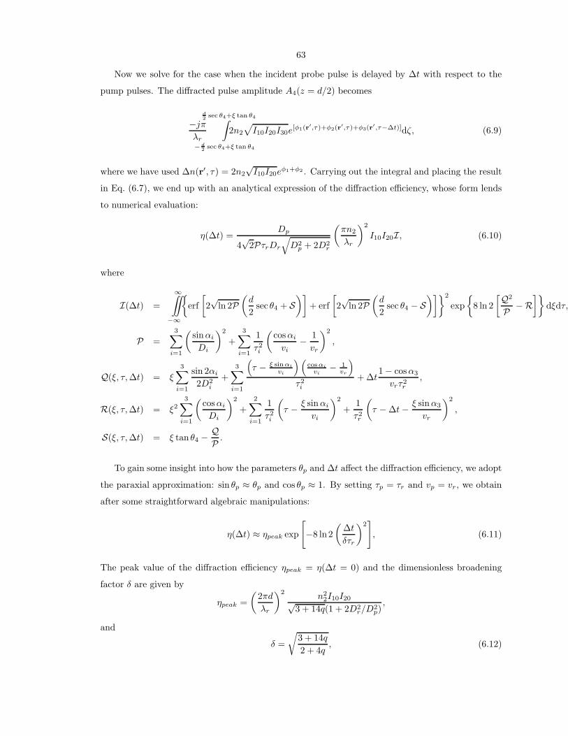
63

Now we solve for the case when the incident probe pulse is delayed by ∆t with respect to the

pump pulses. The diffracted pulse amplitude A4(z = d/2) becomes

−jπ

λr

d2 sec θ4+ξ tan θ4

∫

− d2 sec θ4+ξ tan θ4

2n2

√

I10I20I30e[φ1(r

′,τ)+φ2(r′,τ)+φ3(r

′,τ−∆t)]dζ, (6.9)

where we have used ∆n(r′, τ) = 2n2

√I10I20e

φ1+φ2 . Carrying out the integral and placing the result

in Eq. (6.7), we end up with an analytical expression of the diffraction efficiency, whose form lends

to numerical evaluation:

η(∆t) =Dp

4√

2PτrDr

√

D2p + 2D2

r

(

πn2

λr

)2

I10I20I, (6.10)

where

I(∆t) =

∞∫

−∞

∫{

erf

[

2√

ln 2P(

d

2sec θ4 + S

)]

+ erf

[

2√

ln 2P(

d

2sec θ4 − S

)]}2

exp

{

8 ln 2

[Q2

P −R]}

dξdτ,

P =

3∑

i=1

(

sinαi

Di

)2

+

3∑

i=1

1

τ2i

(

cosαi

vi− 1

vr

)2

,

Q(ξ, τ, ∆t) = ξ

3∑

i=1

sin 2αi

2D2i

+

3∑

i=1

(

τ − ξ sin αi

vi

) (

cos αi

vi− 1

vr

)

τ2i

+ ∆t1 − cosα3

vrτ2r

,

R(ξ, τ, ∆t) = ξ23

∑

i=1

(

cosαi

Di

)2

+

2∑

i=1

1

τ2i

(

τ − ξ sin αi

vi

)2

+1

τ2r

(

τ − ∆t − ξ sin α3

vr

)2

,

S(ξ, τ, ∆t) = ξ tan θ4 −QP .

To gain some insight into how the parameters θp and ∆t affect the diffraction efficiency, we adopt

the paraxial approximation: sin θp ≈ θp and cos θp ≈ 1. By setting τp = τr and vp = vr, we obtain

after some straightforward algebraic manipulations:

η(∆t) ≈ ηpeak exp

[

−8 ln2

(

∆t

δτr

)2]

, (6.11)

The peak value of the diffraction efficiency ηpeak = η(∆t = 0) and the dimensionless broadening

factor δ are given by

ηpeak =

(

2πd

λr

)2n2

2I10I20√3 + 14q(1 + 2D2

r/D2p)

,

and

δ =

√

3 + 14q

2 + 4q, (6.12)

64

Ddiff

Dtrans

CrystalL

L

M

BBO

DSBS1

BS2

M

BC

lr = 776 nm

lp = 388 nm 2qp

x

zy

P

Figure 6.3: Schematic illustration of the holographic pump-and-probe setup. (BC: Berek compen-sator, serving as half-wave plate for the probe pulse; BS: beam splitter; D: photodetector; DS: probedelay stage; L: lens; M: mirror; P: polarizer)

where we have used D = DpDr/√

D2p + 2D2

r , θ1 = −θ2 = θp and q = (Dθp/τrvr)2. The function

η(∆t) gives us a measure of the temporal resolution of the holographic pump-and-probe setup

through the broadening factor δ(θp), which is the ratio between the FWHM of η(∆t) and that of

our probe pulse intensity profile. Although δ(θp) is a monotonically increasing function of θp, it has

a rather narrow range: 1.22 ≤ δ < 1.87 according to Eq. (6.12). It is explicit that the temporal

resolution is not severely affected by the angle of intersection.

The assumption of negligible difference between the pump and probe group velocities, being

applicable to some materials (for instance, CaF2), cannot be justified in the general case. The

velocity difference can result in an additional broadening of η(∆t).

6.3 Experimental results and discussion

Our experimental setup is illustrated in Fig. 6.3. An axially symmetric pulse at λr = 776 nm is

obtained from a Ti:Sapphire amplified laser system CPA-2010 from Clark-MXR, Inc. The temporal

and spatial FWHM of the pulse intensity are measured to be 0.22 psec and 3.5 mm, respectively.

Four percent of the pulse energy is tapped and serves as the probe pulse displaced by a variable

delay stage. The rest of the pulse is passed through a 1-mm-thick BBO (β − BaB2O4) crystal to

generate a pulse at λp = 388 nm, which is split into two identical pump pulses and then focused

down to one-fifth of their original diameter inside the 1 mm thick calcium fluoride sample for more

pronounced nonlinear response. The angle between the pump pulses 2θp is the value “inside” the

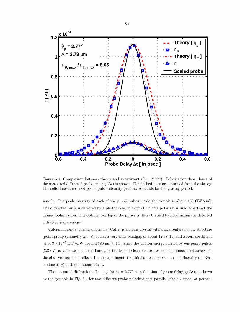
65

−0.6 −0.4 −0.2 0 0.2 0.4 0.60

0.2

0.4

0.6

0.8

1

1.2x 10

−3

Probe Delay ∆t [ in psec ]

η (

∆t )

Theory [ η// ]

η//

Theory [ η⊥ ]

η⊥Scaled probe

θp = 2.77o

Λ = 2.78 µm

η//, max

/ η⊥ , max = 8.65

Figure 6.4: Comparison between theory and experiment (θp = 2.77o). Polarization dependence ofthe measured diffracted probe trace η(∆t) is shown. The dashed lines are obtained from the theory.The solid lines are scaled probe pulse intensity profiles. Λ stands for the grating period.

sample. The peak intensity of each of the pump pulses inside the sample is about 180 GW/cm2.

The diffracted pulse is detected by a photodiode, in front of which a polarizer is used to extract the

desired polarization. The optimal overlap of the pulses is then obtained by maximizing the detected

diffracted pulse energy.

Calcium fluoride (chemical formula: CaF2) is an ionic crystal with a face centered cubic structure

(point group symmetry m3m). It has a very wide bandgap of about 12 eV[13] and a Kerr coefficient

n2 of 3× 10−7 cm2/GW around 580 nm[7, 14]. Since the photon energy carried by our pump pulses

(3.2 eV) is far lower than the bandgap, the bound electrons are responsible almost exclusively for

the observed nonlinear effect. In our experiment, the third-order, nonresonant nonlinearity (or Kerr

nonlinearity) is the dominant effect.

The measured diffraction efficiency for θp = 2.77◦ as a function of probe delay, η(∆t), is shown

by the symbols in Fig. 6.4 for two different probe polarizations: parallel (the η// trace) or perpen-

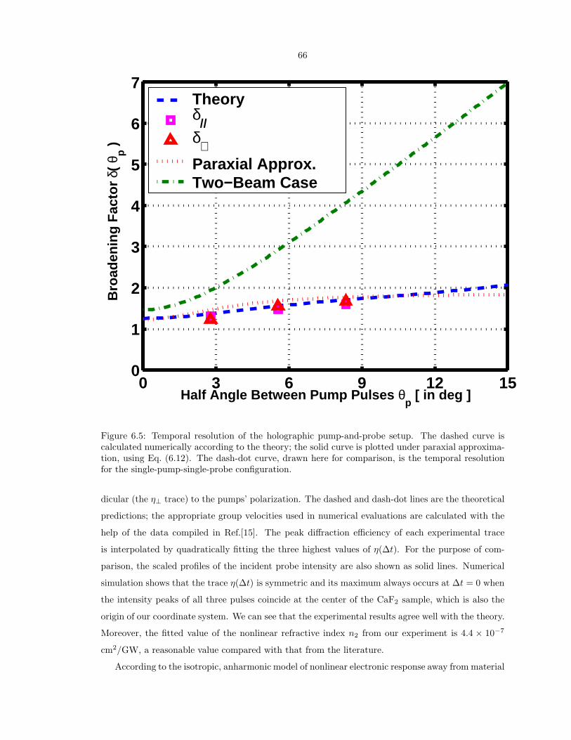
66

0 3 6 9 12 150

1

2

3

4

5

6

7

Half Angle Between Pump Pulses θp [ in deg ]

Bro

aden

ing

Fac

tor

δ( θ

p )

Theory δ

//

δ⊥

Paraxial Approx. Two−Beam Case

Figure 6.5: Temporal resolution of the holographic pump-and-probe setup. The dashed curve iscalculated numerically according to the theory; the solid curve is plotted under paraxial approxima-tion, using Eq. (6.12). The dash-dot curve, drawn here for comparison, is the temporal resolutionfor the single-pump-single-probe configuration.

dicular (the η⊥ trace) to the pumps’ polarization. The dashed and dash-dot lines are the theoretical

predictions; the appropriate group velocities used in numerical evaluations are calculated with the

help of the data compiled in Ref.[15]. The peak diffraction efficiency of each experimental trace

is interpolated by quadratically fitting the three highest values of η(∆t). For the purpose of com-

parison, the scaled profiles of the incident probe intensity are also shown as solid lines. Numerical

simulation shows that the trace η(∆t) is symmetric and its maximum always occurs at ∆t = 0 when

the intensity peaks of all three pulses coincide at the center of the CaF2 sample, which is also the

origin of our coordinate system. We can see that the experimental results agree well with the theory.

Moreover, the fitted value of the nonlinear refractive index n2 from our experiment is 4.4 × 10−7

cm2/GW, a reasonable value compared with that from the literature.

According to the isotropic, anharmonic model of nonlinear electronic response away from material

67

p

p

Wp

k2

k1

Dp

Dp

Wp/sin pp

p

Dp

k2

k1

Dp

Wpy

z

x

Figure 6.6: The concept of the composite pump. The limited longitudinal dimension of femtosecondpulses gives rise to a strip-like region of actual overlap whose width is determined by the pulsetemporal duration as well as the angle of intersection, as shown in the lower part.

resonance, the peak diffraction efficiency of the η// trace is expected to be 9 times as large as that

of the η⊥ trace[7]. In our experiment, this factor turns out to be 8.2 ± 0.4; the discrepancy can be

explained by the deviation from Kleinman’s symmetry[14].

The broadening factor as a function of the half-angle between pump pulses δ(θp) is plotted in

Fig. 6.5: the dashed curve is computed numerically according to the theory, and the solid curve is

plotted using Eq. (6.12) under the assumption of paraxial approximation. Experiments are carried

out for three different values of θp, namely, 2.77◦, 5.55◦ and 8.35◦. We see that the experimental

results closely track the theoretical trend, and δ(θp) almost remains constant for the experiments,

as opposed to the conventional two-beam pump-and-probe setup[10, 9], whose broadening factor is

defined based on the cross-correlation trace of the pump and probe intensities. We reproduce the

two-beam broadening factor (in this case, θp is the half-angle between the pump and probe) as the

dash-dot curve in Fig. 6.5 for the same parameters as used in our holographic experiment.

The key to this almost undegraded temporal resolution in the holographic pump-and-probe

68

setup lies in the concept of “composite pump,” which can be explained with the help of Fig. 6.6. For

simplicity, we consider the case when the pump pulses have rectangular spatial intensity distribution

with transverse and longitudinal dimensions Dp and Wp = vpτp (Wp ≈ 46µm in CaF2 if τp = 220fs).

The overlap of pump pulses is shown in the upper part of the figure as a diamond-shaped region

traced out by dotted lines. As the pump pulses travel and intersect, this region of overlap, the

composite pump, propagates along the z-axis with a velocity vc = vp/ cos θp and has an effective

transverse width of Dc = Wp/ sin θp (shown in the lower part of the figure); this effective width

becomes smaller when θp gets bigger. As evident from the expression, Dc is independent of the

spatial dimension Dp of the pump pulses and solely determined by the pulse temporal duration τp

and the angle of intersection. If we increase the angle 2θp between the pump pulses, the incident

angle θ3 of the probe pulse must also get bigger in order to satisfy the Bragg condition.

Now we can consider the influence of the composite pump on the probe pulse just as in a

two-beam case. Two-beam cross-correlation simulation suggests a broader temporal response for

the increased angular intersection; on the other hand, it produces a narrower temporal response

owing to a shrinking Dc. The reduction in the transverse width of the composite pump constantly

counteracts the effect of an augmented probe incident angle and leaves the temporal resolution in

this configuration almost unchanged.

6.4 Conclusion

With the assumption of an undepleted incident probe pulse, we solved the coupled mode equations

for the femtosecond holography in the case of instantaneous material response. The solution is well

corroborated by the experiments conducted in calcium fluoride crystals. An important implication

of the experimental data obtained for different intersection angles and grating periods is that the

temporal resolution in the holographic pump-and-probe setup is not reduced much by the non-

collinearity. This result will be useful for probing grating-period-dependent mechanisms, such as

diffusion, in materials.

69

Bibliography

[1] Andreas Othonos. Probing ultrafast carrier and phonon dynamics in semiconductors. Appl.

Phys. Rev., 83(4):1789–1830, February 1998.

[2] P. C. Becker, H. L. Fragnito, C. H. B. Cruz, J. Shah, R. L. Fork, J. E. Cunningham, J. E. Henry,

and C. V. Shank. Femtosecond intervalley scattering in GaAs. Appl. Phys. Lett., 53(21):2089–

2090, November 1988.

[3] H. Mahr and M. D. Hirsch. Optical up-conversion light gate with picosecond resolution. Opt.

Commun., 13(2):96–99, 1975.

[4] R. T. Hayes, C. J. Walsh, and M. R. Wasielewski. Using three-pulse femtosecond spec-

troscopy to probe ultrafast triplet energy transfer in zinc meso-tetraarylporphyrin-perylene-

3,4-dicarboximide dyads. J. Phys. Chem. A, 108(16):3253–3260, April 2004.

[5] P. M. Norris, A. P. Caffrey, R. J. Stevens, J. M. Klopf, J. T. McLeskey, and A. N. Smith. Fem-

tosecond pump-probe nondestructive examination of materials. Rev. Sci. Instrum., 74(1):400–

406, January 2003.

[6] Herwig Kogelnik. Coupled wave theory for thick hologram gratings. Bell Syst. Tech. J.,

48(9):2909–2947, November 1969.

[7] R. W. Boyd. Nonlinear Optics. Academic Press, New York, 2nd edition, 2003.

[8] C. L. Thomsen, D. Madsen, S. R. Keiding, J. Thogersen, and O. Christiansen. Two-photon

dissociation and ionization of liquid water studied by femtosecond transient absorption spec-

troscopy. J. Chem. Phys., (7):3453–3462, February 1999.

[9] J. C. Diels and W. Rudolph. Ultrashort Laser Pulse and Phenomena. Academic Press, New

York, 1st edition, 1996.

[10] M. Ziolek, R. Naskrecki, M. Lorenc, J. Karolczak, J. Kubicki, and A. Maciejewski. The influence

of the excitation geometry on the temporal resolution in femtosecond pump-probe experiments.

Opt. Commun., 197(4-6):467–473, October 2001.

70

[11] L. Solymar and D. J. Cooke. Volume Holography and Volume Gratings. Academic Press, New

York, 1981.

[12] M. Born and E. Wolf. Principles of Optics. Cambridge, London, 7th edition, 1999.

[13] M. Huisinga. Ultraviolet Photoelectron Spectroscopy and Electron Stimulated Desorption from

CaF2. PhD thesis, Freie University Berlin, April 1999.

[14] R. T. Lynch, M. D. Levenson, and N. Bloembergen. Experimental test for deviation from

Kleinman’s symmetry in third-order susceptibility tensor. Phys. Lett. A, 50(1):61–62, November

1974.

[15] H. H. Li. Refractive-index of alkaline-earth halide and its wavelength and temperature deriva-

tives. J. Phys. Chem. Ref. Data, 9(1):161–289, 1980.

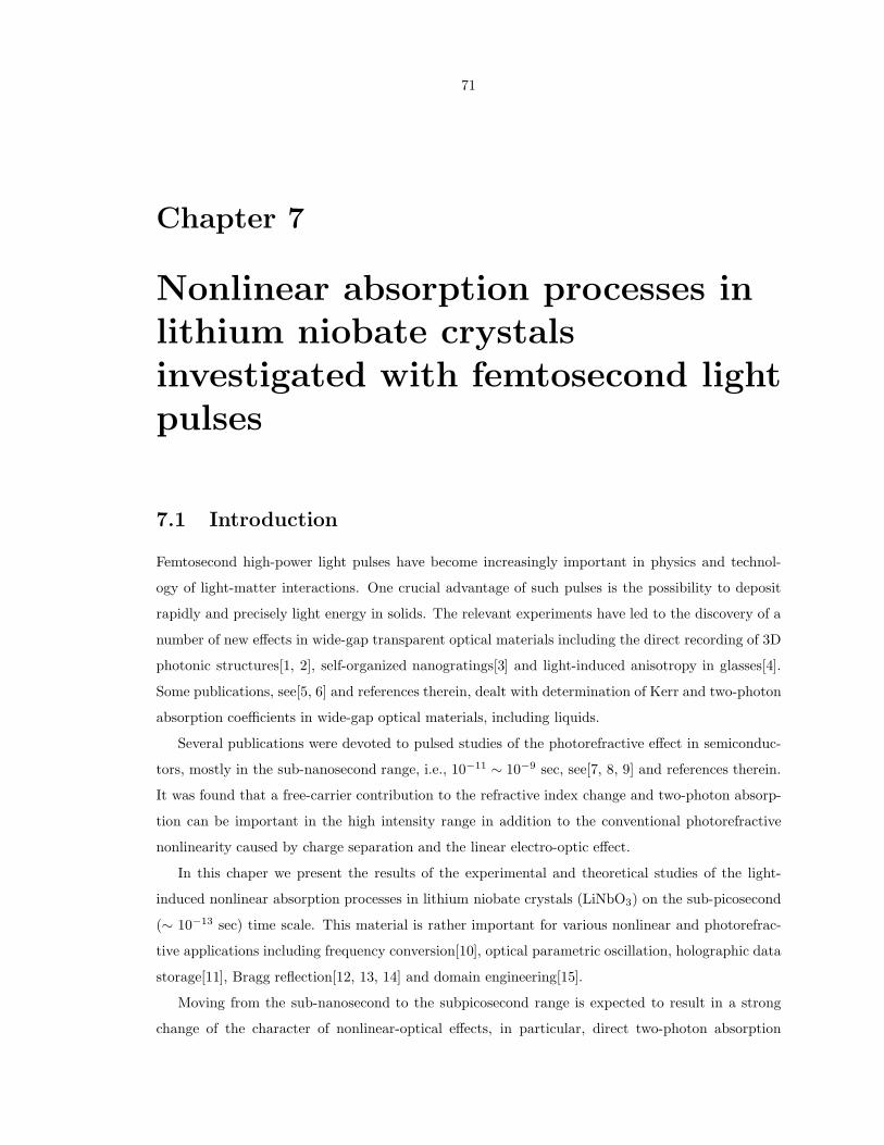
71

Chapter 7

Nonlinear absorption processes in

lithium niobate crystals

investigated with femtosecond light

pulses

7.1 Introduction

Femtosecond high-power light pulses have become increasingly important in physics and technol-

ogy of light-matter interactions. One crucial advantage of such pulses is the possibility to deposit

rapidly and precisely light energy in solids. The relevant experiments have led to the discovery of a

number of new effects in wide-gap transparent optical materials including the direct recording of 3D

photonic structures[1, 2], self-organized nanogratings[3] and light-induced anisotropy in glasses[4].

Some publications, see[5, 6] and references therein, dealt with determination of Kerr and two-photon

absorption coefficients in wide-gap optical materials, including liquids.

Several publications were devoted to pulsed studies of the photorefractive effect in semiconduc-

tors, mostly in the sub-nanosecond range, i.e., 10−11 ∼ 10−9 sec, see[7, 8, 9] and references therein.

It was found that a free-carrier contribution to the refractive index change and two-photon absorp-

tion can be important in the high intensity range in addition to the conventional photorefractive

nonlinearity caused by charge separation and the linear electro-optic effect.

In this chaper we present the results of the experimental and theoretical studies of the light-

induced nonlinear absorption processes in lithium niobate crystals (LiNbO3) on the sub-picosecond

(∼ 10−13 sec) time scale. This material is rather important for various nonlinear and photorefrac-

tive applications including frequency conversion[10], optical parametric oscillation, holographic data

storage[11], Bragg reflection[12, 13, 14] and domain engineering[15].

Moving from the sub-nanosecond to the subpicosecond range is expected to result in a strong

change of the character of nonlinear-optical effects, in particular, direct two-photon absorption

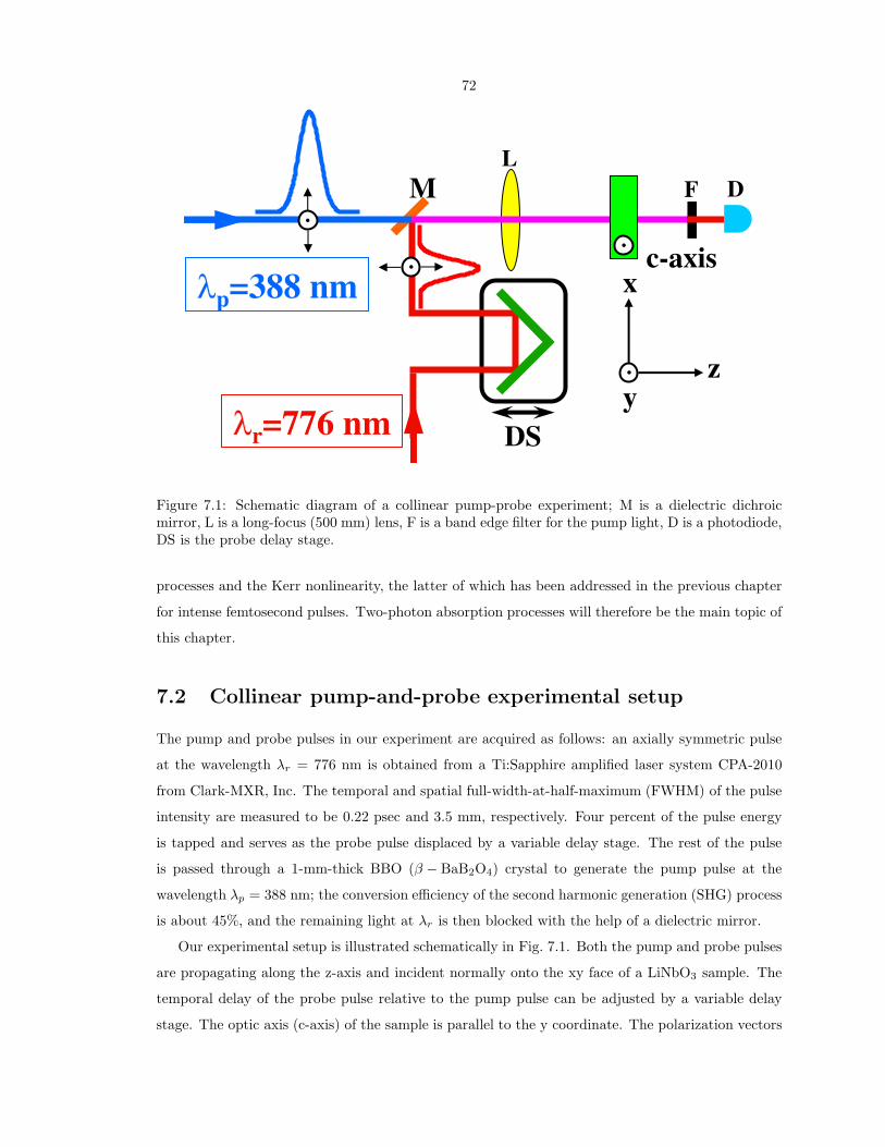
72

r=776 nm

p=388 nm

DS

x

zy

c-axis

L

M F D

Figure 7.1: Schematic diagram of a collinear pump-probe experiment; M is a dielectric dichroicmirror, L is a long-focus (500 mm) lens, F is a band edge filter for the pump light, D is a photodiode,DS is the probe delay stage.

processes and the Kerr nonlinearity, the latter of which has been addressed in the previous chapter

for intense femtosecond pulses. Two-photon absorption processes will therefore be the main topic of

this chapter.

7.2 Collinear pump-and-probe experimental setup

The pump and probe pulses in our experiment are acquired as follows: an axially symmetric pulse

at the wavelength λr = 776 nm is obtained from a Ti:Sapphire amplified laser system CPA-2010

from Clark-MXR, Inc. The temporal and spatial full-width-at-half-maximum (FWHM) of the pulse

intensity are measured to be 0.22 psec and 3.5 mm, respectively. Four percent of the pulse energy

is tapped and serves as the probe pulse displaced by a variable delay stage. The rest of the pulse

is passed through a 1-mm-thick BBO (β − BaB2O4) crystal to generate the pump pulse at the

wavelength λp = 388 nm; the conversion efficiency of the second harmonic generation (SHG) process

is about 45%, and the remaining light at λr is then blocked with the help of a dielectric mirror.

Our experimental setup is illustrated schematically in Fig. 7.1. Both the pump and probe pulses

are propagating along the z-axis and incident normally onto the xy face of a LiNbO3 sample. The

temporal delay of the probe pulse relative to the pump pulse can be adjusted by a variable delay

stage. The optic axis (c-axis) of the sample is parallel to the y coordinate. The polarization vectors

73

0 50 100 150 200 250 300 3500

0.1

0.2

0.3

0.4

0.5

0.6

0.7

0.8

0.9

1

Ip0

[ in GW/cm 2 ]

Tra

nsm

issi

on T

p

d = 1 mmd = 0.5 mmd = 0.07 mm

Figure 7.2: Transmission coeffcient Tp versus peak pump pulse intensity Ip0. The squares, circlesand crosses correspond to the samples 1, 2 and 3, respectively.

of the pulses are separately controlled by specialized half-wave plates (Berek compensators) and are

either parallel or perpendicular to the optic axis. The spatial FWHM of the pulses (after passing

through a converging lens) at the input face is about 0.6 mm. The peak intensity of the pump

pulse Ip0 ranges from ∼ 1 to ∼ 330 GW/cm2. The maximum fluence of the pump pulse is about 79

mJ/cm2. A photo-diode is used to measure the output energy of either the pump or probe pulse by

choosing the proper filter to block one of them out.

Four different samples of LiNbO3, labelled as 1, 2, 3 and 4, are used in the experiments. The

values of the thicknesses d are 1, 0.5, 0.07 and 0.07 mm, respectively. Samples 1, 2 and 3 are

nominally undoped and possess very small (α0 ≤ 0.1 cm−1) linear absorption coefficients at 388 and

776 nm. Sample 4 is iron doped; the iron concentration cFe is about 5.6 × 10−19 cm−3, and the

linear absorption coefficient α0 at 388 nm is about 15 cm−1. For all the samples and wavelengths

used, the linear absorption is negligibly small, i.e., α0d � 1.

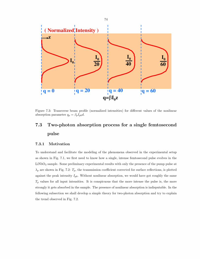
74

q= I0z

q = 0 q = 20 q = 40 q = 60

I0

I0

20

z

( Normalized Intensity )

I0

40

I0

60

Figure 7.3: Transverse beam profile (normalized intensities) for different values of the nonlinearabsorption parameter qp = βpIp0d.

7.3 Two-photon absorption process for a single femtosecond

pulse

7.3.1 Motivation

To understand and facilitate the modeling of the phenomena observed in the experimental setup

as shown in Fig. 7.1, we first need to know how a single, intense femtosecond pulse evolves in the

LiNbO3 sample. Some preliminary experimental results with only the presence of the pump pulse at

λp are shown in Fig. 7.2: Tp, the transmission coefficient corrected for surface reflections, is plotted

against the peak intensity Ip0. Without nonlinear absorption, we would have got roughly the same

Tp values for all input intensities. It is conspicuous that the more intense the pulse is, the more

strongly it gets absorbed in the sample. The presence of nonlinear absorption is indisputable. In the

following subsection we shall develop a simple theory for two-photon absorption and try to explain

the trend observed in Fig. 7.2.

75

7.3.2 Theory of two-photon absorption

We can write down the following equation directly from the Maxwell’s equations under the assump-

tions of negligible beam diffraction and frequency dispersion:

(

∂

∂z+

1

vp

∂

∂t

)

Ip = −βpI2p , (7.1)

where vp = c/np is the pulse velocity in the medium. Eq. (7.1) belongs to a special class of differential

equations called Bernoulli’s equation; it can be solved analytically. The quantity αp = βpIp can be

regarded as the effective absorption coefficient for the pulse, where βp represents the quadratic

absorption coefficient at λp. We have ignored the linear absorption in Eq. (7.1).

The solution to the differential equation Eq. (7.1) subject to the boundary condition at the input

plane z = 0

Ip(x, y, z = 0, t) = Ip0 exp

(

− t2

τ2p

− x2 + y2

D2p

)

is

Ip(x, y, z, t) =Ip0

βpIp0z + exp[

(t−z/vp)2

τ2p

+ x2+y2

D2p

] , (7.2)

where a Gaussian intensity profile of the pulse has been assumed; τp and Dp specify the temporal

and spatial extent of the pulse, respectively. Eq. (7.2) gives a description of the pulse intensity with

the presence of two-photon absorption. If we ride on the top of the pulse as it is propagating inside

the nonlinear medium, i.e., setting t− z/vp = 0, the intensity profile will appear to us as depicted in

Fig. 7.3. We see that the preferential absorption near the center of the pulse results in the flattening

of the Gaussian intensity profile. This flattening effect is more and more obvious as the pulse travels

farther down the road within the medium.

The transmission coefficient Tp is defined as the ratio of the output pulse energy to the input

pulse energy, and for a crystal thickness of d, Tp can be computed from Eq. (7.2) by integrating the

output intensity Ip(x, y, z = d, t) over t and the transverse coordinates x, y and dividing the quantity

by its value at z = 0:

Tp =

∫

∞∫

−∞

∫ Ip0dxdydt

qp+exp

»

(t−d/vp)2

τ2p

+ x2+y2

D2p

–

π√

πτpD2pIp0

,

where qp = βpIp0d is the unitless nonlinear absorption parameter. By making the change of variable

ρ = x2 + y2 and taking advantage of the indefinite integral relation

∫

dx

q + peax=

x

q− 1

aqln (q + peax) ,

76

0 20 40 60 80 1000

0.1

0.2

0.3

0.4

0.5

0.6

0.7

0.8

0.9

1

qp=β

pIp0

d

Pul

se T

rans

mis

sion

Tp

d = 1 mmd = 0.5 mmd = 0.07 mmTheory

Figure 7.4: Dependence of the transmission coefficient Tp on qp = βpIp0d. The dashed curve isplotted from Eq. (7.3). The squares, circles, and crosses represent the experimental data for samples1, 2 and 3, respectively.

we end up with an analytical expression for Tp:

Tp =2

qp√

π

∫ ∞

0

ln(

1 + qpe−t2

)

dt. (7.3)

The transmission coefficient is seen to be determined by a single parameter qp. Plotted as the dashed

curve in Fig. 7.4 is Tp as a function of the variable qp. The curve has a very unique shape: after

a rapid initial fall, the further decrease of Tp occurs very slowly; this is due to the relatively weak

energy absorption at the pulse wings. Even for a high nonlinear absorption parameter, qp = 100,

about 8% of the incident energy is transmitted.

7.3.3 Experimental results

In Fig. 7.4 we also plot the data previously shown in Fig. 7.2 as squares, circles and crosses; only now

the peak intensity Ip0 is incorporated in the parameter qp. The data points have been fitted in accor-

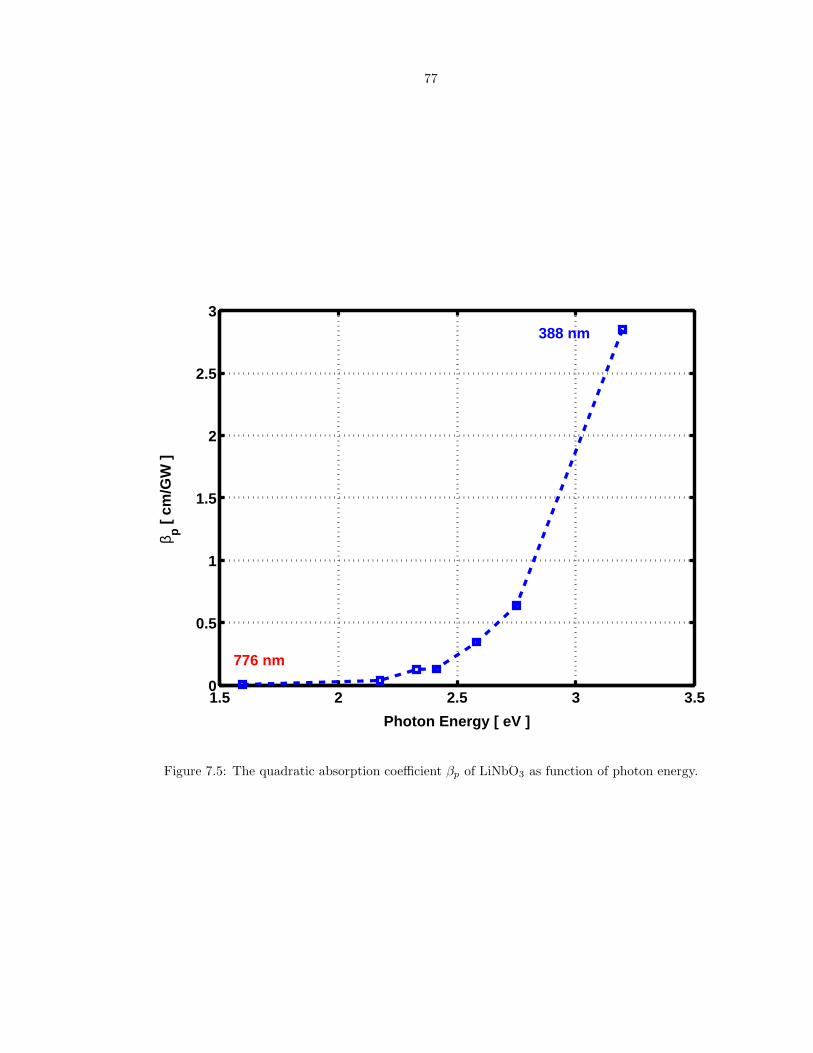
77

1.5 2 2.5 3 3.50

0.5

1

1.5

2

2.5

3

Photon Energy [ eV ]

β p [

cm/G

W ]

776 nm

388 nm

Figure 7.5: The quadratic absorption coefficient βp of LiNbO3 as function of photon energy.

78

−2 −1 0 1 2 3 40.7

0.75

0.8

0.85

0.9

0.95

1

1.05

Probe Delay ∆t [ in psec ]

Nor

mal

ized

Pro

be T

rans

mitt

ance

Tr

Ip0

= 170 GW/cm2

Ip0

= 114 GW/cm2

Ip0

= 83 GW/cm2

Ip0

= 52 GW/cm2

Figure 7.6: Transmission coefficient Tr of the probe pulse versus the time delay ∆t for sample 4 andfour different values of the pump intensity. The circles, squares, crosses, and triangles correspondto Ip0 ∼ 52, 83, 114 and 170 GW/cm2, respectively.

dance with Eq. (7.3), and the value of βp for 388 nm thus extracted is 2.85 cm/GW (corresponding

to a qp value of ∼ 96). The excellent agreement between the data points and the theoretical curve

implies that the two-photon absorption process is indeed the dominant nonlinear effect. In general,

the quadratic absorption coefficient should depend on the light polarization. Our experiments have

shown, however, that the corresponding difference is fairly small, less than 10%.

We also investigate the wavelength dependence of βp: femtosecond pulses at five different wave-

lengths (451 nm, 480 nm, 514 nm, 532 nm and 570 nm) are obtained by passing the seed pulse at 776

nm through a parametric amplifier. The transmission coefficients are measured for all wavelengths,

and the values of βp are fitted just as for the 388 nm pulse. The results are summarized in Fig. 7.5;

βp is plotted as a function of the photon energy in eV. As expected, βp depends rather strongly on

the photon energy: it starts increasing rapidly after ∼ 2.2 eV, which agrees well with the fact that

the bandgap of LiNbO3 is ∼ 4 eV.

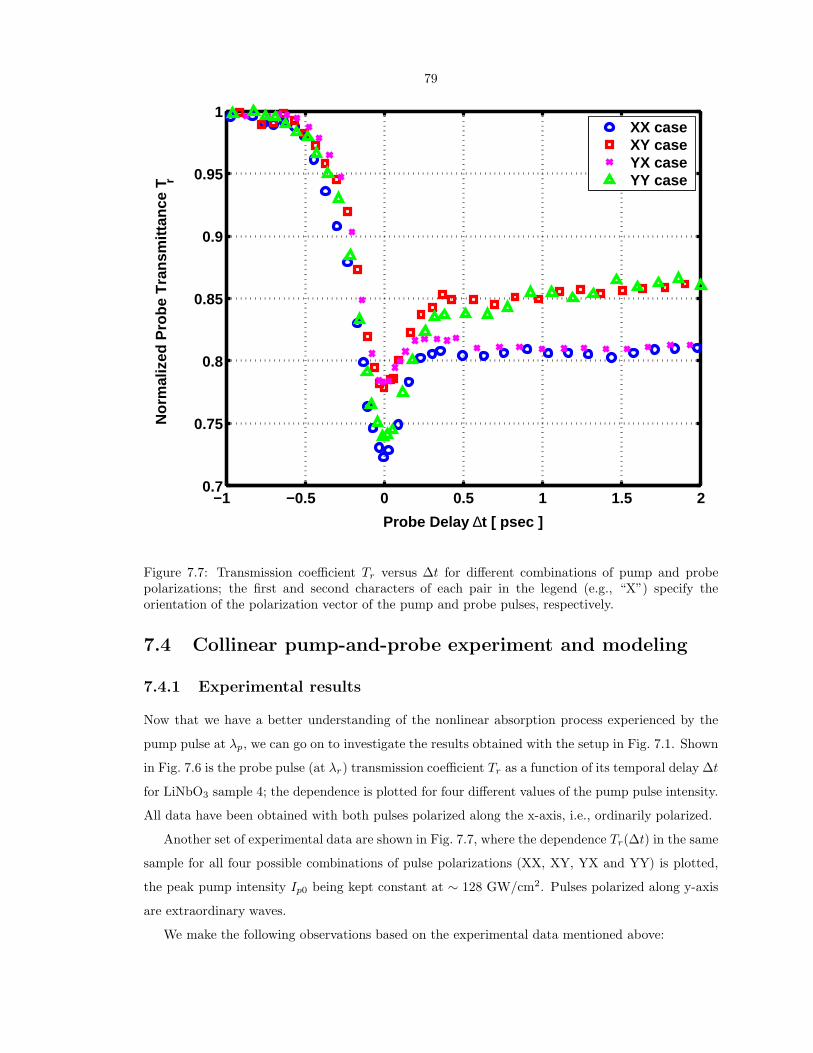
79

−1 −0.5 0 0.5 1 1.5 20.7

0.75

0.8

0.85

0.9

0.95

1

Probe Delay ∆t [ psec ]

Nor

mal

ized

Pro

be T

rans

mitt

ance

Tr

XX caseXY caseYX caseYY case

Figure 7.7: Transmission coefficient Tr versus ∆t for different combinations of pump and probepolarizations; the first and second characters of each pair in the legend (e.g., “X”) specify theorientation of the polarization vector of the pump and probe pulses, respectively.

7.4 Collinear pump-and-probe experiment and modeling

7.4.1 Experimental results

Now that we have a better understanding of the nonlinear absorption process experienced by the

pump pulse at λp, we can go on to investigate the results obtained with the setup in Fig. 7.1. Shown

in Fig. 7.6 is the probe pulse (at λr) transmission coefficient Tr as a function of its temporal delay ∆t

for LiNbO3 sample 4; the dependence is plotted for four different values of the pump pulse intensity.

All data have been obtained with both pulses polarized along the x-axis, i.e., ordinarily polarized.

Another set of experimental data are shown in Fig. 7.7, where the dependence Tr(∆t) in the same

sample for all four possible combinations of pulse polarizations (XX, XY, YX and YY) is plotted,

the peak pump intensity Ip0 being kept constant at ∼ 128 GW/cm2. Pulses polarized along y-axis

are extraordinary waves.

We make the following observations based on the experimental data mentioned above:

80

• The dependence Tr(∆t) has two outstanding features: a dip, which supposedly happens near

∆t = 0, and a quasi-permanent “plateau” after the dip. The temporal width of the dip is

comparable with that of the pulse.

• The value of Tr(∆t) at both the dip and plateau increases with decreasing pump pulse energy.

• A smaller dip transmission T dipr comes about for parallel-polarized pulses (XX and YY) than

for pulses polarized perpendicular to each other.

• The value of Tr at the plateau is determined by the probe polarization; extraordinarily polar-

ized probe experiences a slightly larger plateau transmission T pl.r .

7.4.2 Modeling of collinear pump-and-probe experiment

We attribute the dip manifested by the probe transmission Tr(∆t) to the two-photon absorption

process involving a pump and a probe photon; the sum of the photon energy in this case is ∼ 4.8

eV, which is larger than the band gap of LiNbO3 (∼ 4 eV).

On the other hand, the plateau section in the dependence Tr(∆t) is attributed to the absorption

of the probe pulse by charge carriers (electrons and/or holes) that are excited by the intense pump

pulse; the concentration of the excited free carriers due to pump and probe photons is negligible in

comparison. The polarization dependence of the plateau value is explained by the anisotropy inherent

in the LiNbO3 crystal. We shall model the dip and the plateau sections of Tr(∆t) separately in the

following.

7.4.2.1 Modeling the dip of Tr(∆t)

We can write down the following equation for the probe pulse intensity:

(

∂

∂z+

1

vr

∂

∂t

)

Ir = −βrIpIr . (7.4)

The similarity between Eq. (7.4) and Eq. (7.1) is obvious. The only difference is that the effective

absorption coefficient in Eq. (7.4) is αr = βrIp, which is determined by a much more intense

pump pulse, and βr is the quadratic absorption coefficient characterizing the two-photon absorption

participated by a pump and a probe photon. To solve this equation, it helps to make the change of

variables

ζ = z,

τ = t − zvr

,

after which Eq. (7.4) becomes∂

∂ζIr = −βrIpIr,

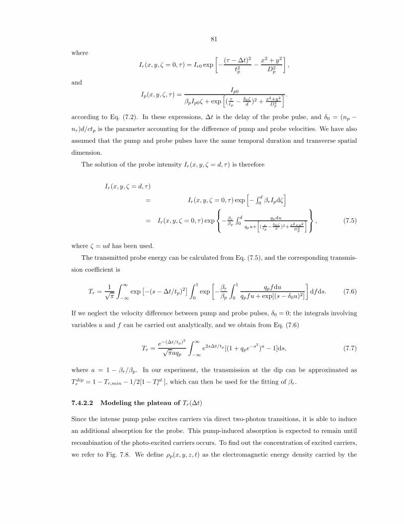
81

where

Ir(x, y, ζ = 0, τ) = Ir0 exp

[

− (τ − ∆t)2

t2p− x2 + y2

D2p

]

,

and

Ip(x, y, ζ, τ) =Ip0

βpIp0ζ + exp[

( τtp

− δ0ζd )2 + x2+y2

D2p

] .

according to Eq. (7.2). In these expressions, ∆t is the delay of the probe pulse, and δ0 = (np −nr)d/ctp is the parameter accounting for the difference of pump and probe velocities. We have also

assumed that the pump and probe pulses have the same temporal duration and transverse spatial

dimension.

The solution of the probe intensity Ir(x, y, ζ = d, τ) is therefore

Ir(x, y, ζ = d, τ)

= Ir(x, y, ζ = 0, τ) exp[

−∫ d

0βrIpdζ

]

= Ir(x, y, ζ = 0, τ) exp

− βr

βp

∫ d

0qpdu

qpu+

»

( τtp

−δ0ζ

d )2+ x2+y2

D2p

–

, (7.5)

where ζ = ud has been used.

The transmitted probe energy can be calculated from Eq. (7.5), and the corresponding transmis-

sion coefficient is

Tr =1√π

∫ ∞

−∞

exp[

−(s − ∆t/tp)2]

∫ 1

0

exp

[

−βr

βp

∫ 1

0

qpfdu

qpfu + exp[(s − δ0u)2]

]

dfds. (7.6)

If we neglect the velocity difference between pump and probe pulses, δ0 = 0; the integrals involving

variables u and f can be carried out analytically, and we obtain from Eq. (7.6)

Tr =e−(∆t/tp)2

√πaqp

∫ ∞

−∞

e2s∆t/tp [(1 + qpe−s2

)a − 1]ds, (7.7)

where a = 1 − βr/βp. In our experiment, the transmission at the dip can be approximated as

T dipr = 1 − Tr,min − 1/2[1 − T pl.

r ], which can then be used for the fitting of βr.

7.4.2.2 Modeling the plateau of Tr(∆t)

Since the intense pump pulse excites carriers via direct two-photon transitions, it is able to induce

an additional absorption for the probe. This pump-induced absorption is expected to remain until

recombination of the photo-excited carriers occurs. To find out the concentration of excited carriers,

we refer to Fig. 7.8. We define ρp(x, y, z, t) as the electromagnetic energy density carried by the

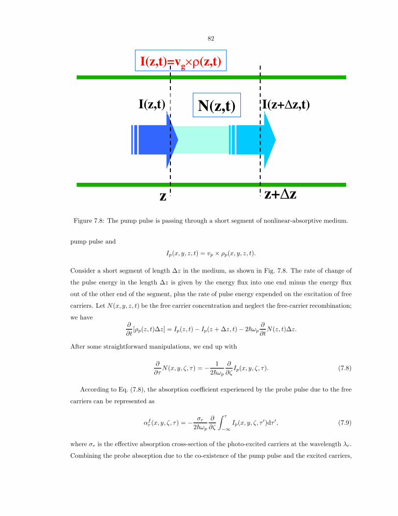
82

z z+ z

N(z,t)I(z,t) I(z+ z,t)

I(z,t)=vg (z,t)

Figure 7.8: The pump pulse is passing through a short segment of nonlinear-absorptive medium.

pump pulse and

Ip(x, y, z, t) = vp × ρp(x, y, z, t).

Consider a short segment of length ∆z in the medium, as shown in Fig. 7.8. The rate of change of

the pulse energy in the length ∆z is given by the energy flux into one end minus the energy flux

out of the other end of the segment, plus the rate of pulse energy expended on the excitation of free

carriers. Let N(x, y, z, t) be the free carrier concentration and neglect the free-carrier recombination;

we have∂

∂t[ρp(z, t)∆z] = Ip(z, t) − Ip(z + ∆z, t) − 2~ωp

∂

∂tN(z, t)∆z.

After some straightforward manipulations, we end up with

∂

∂τN(x, y, ζ, τ) = − 1

2~ωp

∂

∂ζIp(x, y, ζ, τ). (7.8)

According to Eq. (7.8), the absorption coefficient experienced by the probe pulse due to the free

carriers can be represented as

αfr (x, y, ζ, τ) = − σr

2~ωp

∂

∂ζ

∫ τ

−∞

Ip(x, y, ζ, τ ′)dτ ′, (7.9)

where σr is the effective absorption cross-section of the photo-excited carriers at the wavelength λr.

Combining the probe absorption due to the co-existence of the pump pulse and the excited carriers,

83

0 1 2 3 4 50

0.05

0.1

0.15

0.2

0.25

Pump Absorption Parameter qp=β

pIp0

d

[1−T

rdip

] or

[1−T

rplat

eau

]

Dip XXDip YYPlateau XXPlateau YY

Figure 7.9: Dependence of the dip and plateau amplitudes on the product qp = βpIp0d for sample 3and two different pump-probe polarization states. The points are experimental data, and the solidlines are theoretical fits.

we have

Ir(x, y, ζ = d, τ) = Ir(x, y, ζ = 0, τ) exp

[

−∫ d

0

(βrIp + αfr )dζ

]

. (7.10)

To compute T pl.r , consider the case when the pump pulse has already passed through, i.e., the

probe pulse does not overlap with the pump pulse. Mathematically, we set Ip = 0 in Eq. (7.10) and

τ = ∞ in Eq. (7.9) and the plateau value is

T pl.r =

∫ ∞

0

exp

[

−f − bqp

(√π

2e−f −

∫ ∞

0

ds

qp + ef+s2

)]

df, (7.11)

where b = σrtp/~ωpβpd.

84

7.4.3 Comparison between theory and experiments: the determination

of parameters βr and σr

Fig. 7.9 shows the experimental data for the dependence of the dip and plateau amplitudes on

the pump absorption parameter qp, obtained for two different polarization cases, together with the

theoretical fit. The fit parameters are the ratio βr/βp (for the dip amplitude) and b = σrtp/~ωpβpd

(for the plateau amplitude).

The ratio βr/βp deduced from the fitting procedure is ∼ 0.23 for the XX case and ∼ 0.24 for the

YY case. Thus, with an accuracy of (10 ∼ 15)%, the value of βr can be estimated as ∼ 0.67 cm/GW.

The values of b can be estimated as ∼ 0.21 and ∼ 0.14 for the XX and YY cases, respectively. This

gives us the values of the excitation cross-section: σr,xx ∼ 1.60×10−17 cm2 and σr,yy ∼ 1.08×10−17

cm2.

7.5 Conclusion

Propagation of high-power femtosecond light pulses in lithium niobate crystals (LiNbO3) is inves-

tigated experimentally and theoretically in collinear pump-and-probe transmission experiments. It

is found that within a wide intensity range a strong decrease of the pump transmission coefficient

at 388 nm fully complies with the model of two-photon absorption; the corresponding nonlinear ab-

sorption coefficient is βp ≈ 2.85 cm/GW. Furthermore, intense pump pulses induce a considerable

absorption for a probe pulse at 776 nm. The dependence of the probe transmission coefficient on

the time delay ∆t between probe and pump pulses is characterized by a narrow dip (at ∆t ≈ 0) and

a long (on the picosecond time scale) lasting plateau. The dip is due to direct two-photon transi-

tions involving both pump and probe photons; the corresponding nonlinear absorption coefficient is

βr ≈ 0.67 cm/GW. The plateau absorption is caused by the presence of free carriers excited by the

pump pulse; the effective absorption cross-section at 776 nm is σr ≈ 1.60 × 10−17 cm2. The above

nonlinear absorption parameters are not strongly polarization sensitive. No specific manifestations

of the relaxation of hot carriers are found for a pulse duration of about 0.22 ps. From the obtained

results it becomes clear that two-photon absorption will strongly affect holographic recording in

LiNbO3 with ultrashort intense light pulses.

85

Bibliography

[1] K. Miura, J. R. Qiu, H. Inouye, T. Mitsuyu, and K. Hirao. Photowritten optical waveguides in

various glasses with ultrashort pulse laser. Applied Physics Letters, 71(23):3329–3331, December

1997.

[2] J. D. Mills, P. G. Kazansky, E. Bricchi, and J. J. Baumberg. Embedded anisotropic microreflec-

tors by femtosecond-laser nanomachining. Applied Physics Letters, 81(2):196–198, July 2002.

[3] Y. Shimotsuma, P. G. Kazansky, J. R. Qiu, and K. Hirao. Self-organized nanogratings in glass

irradiated by ultrashort light pulses. Physical Review Letters, 91(24):247405, December 2002.

[4] P. G. Kazansky, H. Inouye, T. Mitsuyu, K. Miura, J. Qiu, K. Hirao, and F. Starrost. Anomalous

anisotropic light scattering in Ge-doped silica glass. Physical Review Letters, 82(10):2199–2202,

March 1999.

[5] R. DeSalvo, A. A. Said, D. J. Hagan, E. W. VanStryland, and M. SheikBahae. Infrared to

ultraviolet measurements of two-photon absorption and n(2) in wide bandgap solids. IEEE

Journal of Quantum Electronics, 32(8):1324–1333, August 1996.

[6] A. Dragonmir, J. G. McInerney, and D. N. Nikogosyan. Femtosecond measurements of two-

photon absorption coefficients at λ=264 nm in glasses, crystals, and liquids. Applied Optics,

41(21):4365–4376, July 2002.

[7] H. J. Eichler, P. Gunter, and D. W. Pohl. Laser-Induced Dynamic Gratings. Springer-Verlag,

New York, 1986.

[8] A. L. Smirl, G. C. Valley, K. M. Bohnert, and T. F. Boggess. Picosecond photorefractive and

free-carrier transient energy-transfer in GaAs at 1 µm. IEEE Journal of Quantum Electronics,

24(23):289–303, February 1988.

[9] G. C. Valley, J. Dubard, and A. L. Smirl. Theory of high-gain transient energy-transfer in GaAs

and Si. IEEE Journal of Quantum Electronics, 26(6):1058–1066, June 1990.

[10] M. Centini, C. Sibilia, M. Scalora, G. D’Aguanno, M. Bertolotti, M. J. Bloemer, C. M. Bowden,

and I. Nefedov. Dispersive properties of finite, one-dimensional photonic band gap structures:

86

applications to nonlinear quadratic interactions. Physical Review E, 60(4):4891–4898, October

1999.

[11] H. J. Coufal, D. Psaltis, and G. T. Sincerbox. Holographic Data Storage. Springer-Verlag, New

York, 2000.

[12] P. Boffi, D. Piccinin, and M. C. Ubaldi. Infrared Holography for Optical Communications.

Springer-Verlag, New York, 2003.

[13] G. A. Rakuljic and V. Leyva. Volume holographic narrow-band optical filter. Optics Letters,

18:459–461, March 1993.

[14] S. Breer and K. Buse. Wavelength demultiplexing with volume phase holograms in photore-

fractive lithium niobate. Applied Physics B, 66:339–345, March 1998.

[15] J. P. Meyn and M. M. Fejer. Tunable ultraviolet radiation by second-harmonic generation in

periodically poled lithium tantalate. Optics Letters, 22(16):1214–1216, August 1997.

87

Chapter 8

Femtosecond recording of spatial

gratings and time-resolved readout

in lithium niobate

8.1 Introduction

Ferroelectric lithium niobate is one of the most investigated man-made materials for its widespread

and promising applications in integrated and nonlinear optics[1], e.g., parametric amplification, sec-

ond harmonic generation[2] (SHG) and periodically-poled lithium niobate[3] (PPLN). Its superior

photorefractive property[4], which is characterized by the change in refractive index resulting from

the optically induced redistribution of electrons and/or holes and the linear electro-optic effect[5],

has made lithium niobate (LiNbO3) an extremely attractive candidate for many applications such as

holographic data storage, optical information processing, phase conjugation, beam steering, telecom-

munication switching and WDM filters[6, 7, 8, 9], just to name a few.

The photorefractive effect is a peculiar form of the (second-order) optical nonlinearity in the

sense that it cannot be described by a nonlinear susceptibility χ(n) that is utilized extensively to

characterize almost all optical nonlinearities; this peculiarity comes from the fact that the induced

index change in photorefractive materials is not an instantaneous effect proportional to the product

of participating light intensities but a delayed response depending on such diverse parameters as

sample doping impurities, dopant concentration and oxidation/reduction states, grating period,

photovoltaic effect, light intensity, etc.

The distinction between the photorefractive effect and the other inherent nonlinearities will

need to be addressed when the holographic recording is performed with high-intensity laser pulses.

Grating-recording experiments have been conducted extensively in lithium niobate in the past few

decades at low-intensity (≤ 103 W/m2), mainly associated with continuous-wave laser, and high-

intensity (up to ∼ 1011 W/m2) made possible by nanosecond pulses[10, 11]. Jermann and Otten[10]

88

made use of the two-center model to successfully explain the increased recording sensitivity and

saturation value of the index modulation at elevated recording light intensity. At these intensity

levels, the photorefractive effect is still the dominant nonlinear effect; however, it is conceivable that

holographic recording with even more intense (picosecond or even shorter) pulses will inevitably

enhance and reveal other nonlinear material responses.

Picosecond pulses with peak intensity 1012 to 1013 W/m2 have been used to investigate the ph-

torefractive and beam-coupling effects in various materials, e.g., GaAs[12, 13, 14], BSO (Bi12SiO20)[15],

barium titanate (BaTiO3)[16], potassium niobate (KNbO3)[17], etc. These experiments are con-

ducted with pump-probe techniques that include two intense, interfering pump pulses responsible

for establishing index and/or absorption gratings and a weak, Bragg-matched probe pulse that gets

diffracted by the grating. The measured responses consist of an initial instantaneous peak followed by

a permanent (“left-over”) photorefractive grating. The source of the initial peaks remains ambiguous

owing to the temporal resolution limit in these experiments. Among various possible contributing

mechanisms to the initial diffraction peak are degenerate four-wave mixing (due to instantaneous

third-order nonlinearity) and free carrier gratings (due to modulated concentration of excited charge

carriers).

In this chapter we will employ femtosecond pulses with peak intensity up to 3 × 1015 W/m2 to

pump and probe LiNbO3 samples. Enhanced temporal resolution in the experiment and accumu-

lated knowledge from the previous two chapters enable us to draw conclusions from the observed

phenomena and help shed light on the involved nonlinear processes.

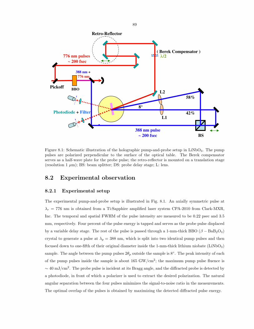
89

42%

388 nm pulse

~ 200 fsec BS

58%

8

•

Retro-Reflector

Photodiode + Filter

776 nm pulses

~ 200 fsec

BBO

388 nm +

776 nm

L1

L2Pickoff

/2( Berek Compensator )

Figure 8.1: Schematic illustration of the holographic pump-and-probe setup in LiNbO3. The pumppulses are polarized perpendicular to the surface of the optical table. The Berek compensatorserves as a half-wave plate for the probe pulse; the retro-reflector is mounted on a translation stage(resolution 1 µm); BS: beam splitter; DS: probe delay stage; L: lens.

8.2 Experimental observation

8.2.1 Experimental setup

The experimental pump-and-probe setup is illustrated in Fig. 8.1. An axially symmetric pulse at

λr = 776 nm is obtained from a Ti:Sapphire amplified laser system CPA-2010 from Clark-MXR,

Inc. The temporal and spatial FWHM of the pulse intensity are measured to be 0.22 psec and 3.5

mm, respectively. Four percent of the pulse energy is tapped and serves as the probe pulse displaced

by a variable delay stage. The rest of the pulse is passed through a 1-mm-thick BBO (β − BaB2O4)

crystal to generate a pulse at λp = 388 nm, which is split into two identical pump pulses and then

focused down to one-fifth of their original diameter inside the 1-mm-thick lithium niobate (LiNbO3)

sample. The angle between the pump pulses 2θp outside the sample is 8◦. The peak intensity of each

of the pump pulses inside the sample is about 165 GW/cm2; the maximum pump pulse fluence is

∼ 40 mJ/cm2. The probe pulse is incident at its Bragg angle, and the diffracted probe is detected by

a photodiode, in front of which a polarizer is used to extract the desired polarization. The natural

angular separation between the four pulses minimizes the signal-to-noise ratio in the measurements.

The optimal overlap of the pulses is obtained by maximizing the detected diffracted pulse energy.

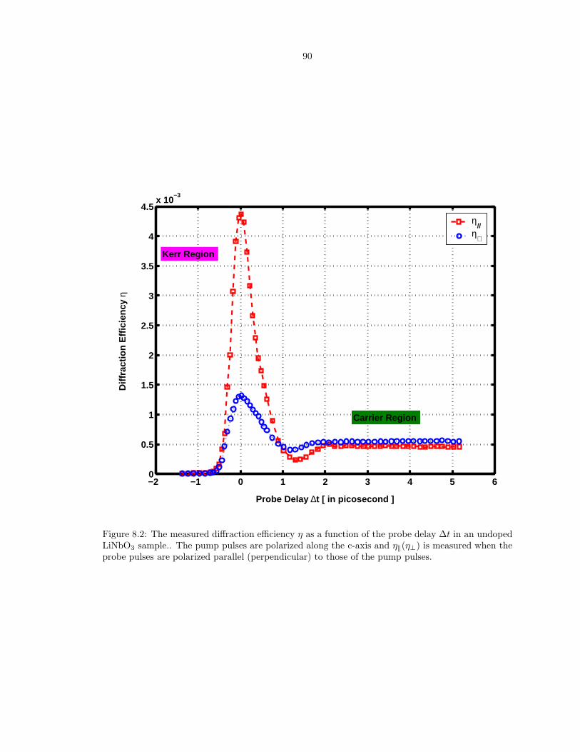
90

−2 −1 0 1 2 3 4 5 60

0.5

1

1.5

2

2.5

3

3.5

4

4.5x 10

−3

Probe Delay ∆t [ in picosecond ]

Diff

ract

ion

Effi

cien

cy

η

η//

η⊥

Kerr Region

Carrier Region

Figure 8.2: The measured diffraction efficiency η as a function of the probe delay ∆t in an undopedLiNbO3 sample.. The pump pulses are polarized along the c-axis and η‖(η⊥) is measured when theprobe pulses are polarized parallel (perpendicular) to those of the pump pulses.

91

8.2.2 Polarization dependence

The polarization dependence of the measured diffraction efficiency η is shown in Fig. 8.2, where

two configurations denoted by η‖ (in squares) and η⊥ (in circles) are plotted. The experiment is

carried out with the c-axis of a undoped LiNbO3 crystal orientated parallel to the polarization

of the pump pulses. The data of η‖(η⊥) are acquired when the polarization of the probe pulses,

adjusted with the help of the Berek compensator and a polarizer in front of the photo-detector, is

parallel (perpendicular) to that of the pump pulses. The position of the origin ∆t = 0 is determined

by quadratically fitting the three data points corresponding to the highest measured diffraction

efficiencies; the origin is then assigned the position where the fitted maximum occurs (since the

material response is assumed to be instantaneous[5]). Every data point corresponds to the value of

the measured diffraction efficiency averaged over 100 single-pulse experiments: after each pump-and-

probe measurement, uniform illumination is applied to erase the remnant photorefractive grating.

Both curves in Fig. 8.2 show a very distinctive set of features when the probe delay ∆t is gradually

increased:

1. The diffraction efficiency increases rapidly toward a peak value (ηpeak), which occurs when the

probe pulses supposedly has the maximum overlap with the pump pulses. The value of ηpeak,‖

is significantly larger than ηpeak,⊥, about 3 times.

2. After it has peaked, the diffraction efficiency then decreases rapidly, albeit at a less steep rate

than when it ascends.

3. When ∆t ≥ 2 picosecond, the value of η remains constant at a “plateau” value ηpl. well into

almost 1 nanosecond. The value of ηpl.,‖ is only slightly smaller than that of ηpl.,⊥.

4. The transition between the descending η and the constant η is a very interesting “valley”

region between ∆t = 1 and 2 picosecond; i.e., η dips under ηpl. and then climbs back to the

ηpl. level.

A detectable permanent photorefractive grating is present after the illumination of a few pump pulses

without erasure; this grating can be easily erased with a uniform light source. Uniform illumination

after each pump-and-probe attempt ensures a clean slate for the next measurement.

Based on the experiments done in and knowledge accumulated from the previous two chapters,

we attribute the diffracted probe pulse around ηpeak to the instantaneous mixed grating as a result

of the Kerr effect and two-photon absorption involving both the pump and probe photons. On the

other hand, the semi-permanent component ηpl. is associated with the carriers excited by the intense

pump pulses. The concentration of the carriers is modulated after the interfering pump pulses and

therefore constitute another mixed grating by which the much delayed probe pulse gets diffracted.

92

The “valley” feature of η has to be a joint product of the two mixed gratings. A little thought

points to the “negative” index of the carrier grating. The “valley” can only be present when the

two index gratings due to the Kerr effect and excited carriers cancel each other; after the Kerr index

grating disappears, η slightly increases to the ηpl. level. At the bottom of the η valley, the two index

gratings cancel each other completely, and the diffracted energy is dedicated to the two absorption

gratings, which are additive.

93

−2 −1 0 1 2 3 4 5 60

0.2

0.4

0.6

0.8

1

1.2

1.4x 10

−3

Probe Delay ∆t [ in picosecond ]

Diff

ract

ion

Effi

cien

cy

LiNbO3, undoped

LiNbO3:Fe

LiNbO3:Mn

Figure 8.3: The measured diffraction efficiency η as a function of the probe delay ∆t in undoped(circles), iron-doped (triangles) and manganese-doped (squares) LiNbO3 samples. The pump pulsesare polarized along the c-axis, and all measurements are carried out in the η⊥) configuration.

8.2.3 Dependence on dopants

In Fig. 8.3, the experimental data of η(∆t) for an undoped and two impurity-doped LiNbO3 crystals

are plotted together for comparison. The doped impurities do not strongly influence the behavior

in the pump-and-probe experiment, which corroborates that the probe pulse is diffracted because

of the intrinsic attributes present in the LiNbO3 matrix rather than mechanisms brought about by

dopants or impurities.

94

d

z

x

Pump

Pump

Probe

2

1

2

3

4

4

Diffracted

Probe

1

3

Figure 8.4: Configuration of the femtosecond holographic experiment in lithium niobate; 1 and 2are the pump (recording) pulses, while 3 and 4 are the probe and diffracted pulses.

8.3 Theoretical justification and comparison with experimen-

tal data

In Fig. 8.4, the interference between the two intense pump pulses results in a modulated intensity

pattern:

I(x, y, z, t) = I1 + I2 + 2√

I1I2 cosKx.

The intensities of these pulses inside lithium niobate can therefore be described by the following

nonlinear coupled equations:

(

s1 · ∇ +1

vp

∂

∂t

)

I1 = −βpI1

(

I1 + I2 + 2√

I1I2 cosKx)

, (8.1a)

(

s2 · ∇ +1

vp

∂

∂t

)

I2 = −βpI2

(

I1 + I2 + 2√

I1I2 cosKx)

, (8.1b)

where βp is the material nonlinear absorption coefficient at 388 nm. As seen by the probe pulse

3, the modulated intensity pattern I(x, y, z, t) gives rise to a mixed grating, which comprises the

following components:

95

1. An index modulation

∆n(x, y, z, t) cosKx = 2n2

√

I1I2 cosKx

owing to the optical Kerr effect; here K = 2k1 sin θ1, and n2 is the appropriate Kerr coefficient.

2. An absorption grating

α + ∆α(x, y, z, t) cosKx = βr

(

I1 + I2 + 2√

I1I2 cosKx)

owing to the two-photon transition involving pump and probe photons; here βr is the corre-

sponding nonlinear absorption coefficient, and α and ∆α are absorption constants applicable

to the pulse intensity.

The probe pulse gets diffracted by this mixed grating and coupled into the diffracted pulse 4; the

amplitudes of these two pulses obey the following coupled mode equations when the Bragg condition

is satisfied:

(

s3 · ∇ +1

vr

∂

∂t

)

A3 = −α

2A3 − jκA4, (8.2a)

(

s4 · ∇ +1

vr

∂

∂t

)

A4 = −α

2A4 − jκA3, (8.2b)

where vr is the group velocity of the probe pulse and

κ =π∆n

λr− j

∆α

4(8.3)

is the coupling constant as a result of the mixed grating.

8.3.1 Decoupling of pump pulses when qp = 2βpIp0d ≤ 1

To simplify the computations, we consider the case when the initial peak pump intensities Ip0 satisfy

2βpIp0d ≤ 1; in this case, the coupling effects between the pump pulses as described by Eqs. (8.1a)

and (8.1b) become unimportant, and we can solve analytically for the pump pulses subject to the

condition that they possess Gaussian profiles before entering the nonlinear medium:

Ii(x, y, z, t) =Ip0

2βpIp0

(

z + d2

)

sec θi + exp

[

“

t−z cos θi+x sin θi

vp

”2

τ2p

+ (x cos θi−z sin θi)2+y2

D2p

] , (8.4)

where i = 1, 2 and τp and Dp are the parameters characterizing the pulses’ temporal and spatial

widths.

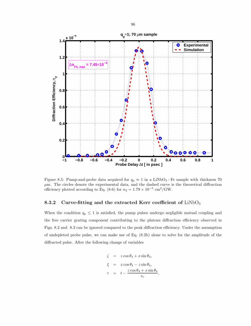
96

−1 −0.8 −0.6 −0.4 −0.2 0 0.2 0.4 0.6 0.8 10

0.2

0.4

0.6

0.8

1

1.2

1.4x 10

−4

Probe Delay ∆t [ in psec ]

Diff

ract

ion

Effi

cien

cy,

η //

qp≈1; 70 µm sample

ExperimentalSimulation

∆nFit, max

= 7.45×10−4

Figure 8.5: Pump-and-probe data acquired for qp ≈ 1 in a LiNbO3 : Fe sample with thickness 70µm. The circles denote the experimental data, and the dashed curve is the theoretical diffractionefficiency plotted according to Eq. (8.6) for n2 = 1.79 × 10−5 cm2/GW.

8.3.2 Curve-fitting and the extracted Kerr coefficient of LiNbO3

When the condition qp ≤ 1 is satisfied, the pump pulses undergo negligible mutual coupling and

the free carrier grating component contributing to the plateau diffraction efficiency observed in

Figs. 8.2 and 8.3 can be ignored compared to the peak diffraction efficiency. Under the assumption

of undepleted probe pulse, we can make use of Eq. (8.2b) alone to solve for the amplitude of the

diffracted pulse. After the following change of variables

ζ = z cos θ4 + x sin θ4,

ξ = x cos θ4 − z sin θ4,

τ = t − z cos θ4 + x sin θ4

vr,

97

Eq. (8.2b) turns into∂

∂ζA4(ξ, y, ζ, τ) = −jκ(ξ, y, ζ, τ)A3(ξ, y, ζ, τ),

where the coupling constant κ only consists of the instantaneous components (namely, Kerr effect

and nonlinear absorption of the probe photons at the presence of pump photons).

The boundary condition A4

(

ζ = − d2 sec θ4 + ξ tan θ4

)

= 0 leads to the solution at the exit bound-

ary z = d/2:

A4

(

ξ, y, ζ =d

2sec θ4 + ξ tan θ4, τ

)

= −[

βr

2+ j

2πn2

λr

]

d2 sec θ4+ξ tan θ4

∫

− d2 sec θ4+ξ tan θ4

√

I1I2A3dζ, (8.5)

where the pump pulse profiles from Eq. (8.4) are used.

The amplitude of the probe pulse temporally delayed by ∆t can be represented as

A3(ξ, y, ζ, τ) =√

I30 exp

{

− [τ − ∆t − (ζ cosα3 − ζ + ξ sin α3)/vr]2

2τ2r

− (ξ cosα3 − ζ sin α3)2 + y2

2D2r

}

,

where α3 = θ3 − θ4 and τr and Dr characterize the probe pulse’s temporal and spatial widths. Now

we can compute the diffraction efficiency, which is defined as the energy ratio between the diffracted

pulse and transmitted pulse:

η(∆t) =

∫

∞∫

−∞

∫

|A4(ζ = d2 sec θ4 + ξ tan θ4)|2dξdydτ

π√

πτpD2pI30

. (8.6)

The diffraction efficiency as expressed by Eq. (8.6) is derived for the case qp ≤ 1. To achieve

qp ≤ 1 experimentally, we replace the thick (1-mm) sample with a thin (70-µm) LiNbO3 : Fe sample

(sample 4 as in the previous chapter, with cFe ≈ 5.6× 1019 cm−3 and a linear absorption coefficient

α0 ≈ 15 cm−1 at 388 nm) and attenuate the pump pulse with a proper neutral density filter, bringing

the value of the nonlinear absorption parameter qp down to ∼ 1.

The data obtained from pumping and probing the thin sample are shown as circles in Fig. 8.5;

the polarizations of both the pump and probe pulses are parallel to the c-axis of the LiNbO3 crystal.

As evident from the figure, we have negligible plateau diffraction efficiency from the excited free

carriers; the peak diffraction efficiency can be attributed to the mixed grating characterized by the

two material constants βr and n2. The value of βr in this configuration has been extracted from

the collinear pump-and-probe experiment to be ∼ 0.67 cm/GW. With only n2 as an unknown for

Eq. (8.6), it is straightforward to find its value from Fig. 8.5.

The peak diffraction efficiency can be interpolated from the experimental data by quadratically

fitting the data points corresponding to the three maximum η(∆t) values, producing ηpeak ≈ 1.34×

98

10−4. The dashed curve in Fig. 8.5 is plotted by setting

√

(

πn2

λr

)2

+

(

βr

4

)2

Ip0 ≈ 15 cm−1,

which results in a peak diffraction efficiency η(∆t = 0) = ηpeak. Substituting βr = 0.67 cm/GW, we

end up with n2,‖ ≈ 1.79 × 10−5 cm2/GW for LiNbO3.

The index grating arising from the Kerr effect accounts for almost 95% of the peak diffraction

efficiency η(∆t = 0), which agrees well with the polarization dependence shown in Fig. 8.2: the

dramatic polarization dependence of η(∆t) is an obvious manifestation of the dominant role the Kerr

grating plays in the mixed grating since in both cases the absorption gratings have approximately

equal strengths. As a result, the other Kerr coefficient of interest n2,⊥ can be approximated as

≈ 1.12 × 10−5 cm2/GW.

8.3.3 Mixed grating due to the excited carriers

In addition to the instantaneous mixed grating, a permanent mixed grating attributed to the excited

carriers also exists. To calculate ηpl., we consider the case when the probe pulse is much delayed

and has little overlap with the pump pulses. In Fig. 8.5, a probe delay ∆t of 0.6 psec will suffice.

As in the previous section, we take advantage of the condition qp ≤ 1; neglecting the DC term α,

Eq. (8.2b) becomes

(

s4 · ∇ +1

vr

∂

∂t

)

A4 = −[

jπ

λr

%r

~ωp+

σr

4~ωp

]

∂

∂z

d/2∫

−d/2

∞∫

−∞

√

I1I2dτdz

A3, (8.7)

where σr is the effective absorption cross section of the excited carriers and the parameter %r (having

the unit of volume) characterizes the index change due to the excited carriers at the probe wavelength

λr. A negative index change results in a negative %r.

To have an estimation of the value of ηpl., we adopt the approximation: θ1 = θ2 = θ3 = θ4 = 0,

which is reasonable near the paraxial region. The plateau diffraction efficiency is then calculated

from Eq. (8.7):

ηpl. ≈4√

2

25

(

τpIp0

~ωp

)2 (

π2%2r

λ2r

+σ2

r

16

)

J , (8.8)

where the definite integral

J =

∫ ∞

0

e−s25

[√π

2e−s −

∫ ∞

0

dτ

qp + es+τ2

]2

ds,

and it can be numerically evaluated to be ∼ 3.23842 × 10−2 for qp = 0.9, which corresponds to

the data shown in Fig. 8.5. The diffraction efficiency in this case is ηpl. = 4.8 × 10−6; we know

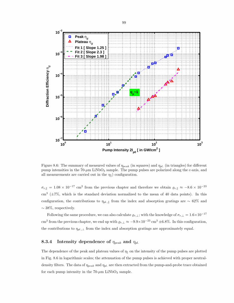
99

100

101

102

103

10−7

10−6

10−5

10−4

10−3

10−2

Pump Intensity 2Ip0

[ in GW/cm 2 ]

Diff

ract

ion

Effi

cien

cy

η //

Peak η//

Plateau η//

Fit 1 [ Slope 1.25 ]Fit 2 [ Slope 2.3 ] Fit 3 [ Slope 1.98 ]

qp≈1

Figure 8.6: The summary of measured values of ηpeak (in squares) and ηpl. (in triangles) for differentpump intensities in the 70-µm LiNbO3 sample. The pump pulses are polarized along the c-axis, andall measurements are carried out in the η‖) configuration.

σr,‖ = 1.08 × 10−17 cm2 from the previous chapter and therefore we obtain %r,‖ ≈ −8.6 × 10−23

cm3 (±7%, which is the standard deviation normalized to the mean of 40 data points). In this

configuration, the contributions to ηpl.,‖ from the index and absorption gratings are ∼ 62% and

∼ 38%, respectively.

Following the same procedure, we can also calculate %r,⊥; with the knowledge of σr,⊥ = 1.6×10−17

cm2 from the previous chapter, we end up with %r,⊥ ≈ −9.9×10−23 cm3 ±6.8%. In this configuration,

the contributions to ηpl.,⊥ from the index and absorption gratings are approximately equal.

8.3.4 Intensity dependence of ηpeak and ηpl.

The dependence of the peak and plateau values of η‖ on the intensity of the pump pulses are plotted

in Fig. 8.6 in logarithmic scales; the attenuation of the pump pulses is achieved with proper neutral-

density filters. The data of ηpeak and ηpl. are then extracted from the pump-and-probe trace obtained

for each pump intensity in the 70-µm LiNbO3 sample.

100

The dependence of ηpl.(Ip0) is fitted with the function ηpl.(Ip0) = aIbp0. The extracted optimal

exponent b is ∼ 2 for the cases qp > 10, which can be justified as follows: when qp > 10, most of the

pump energy is absorbed, and the absorbed pulse energy is proportional to the concentration of the

excited carriers, which is responsible for the diffraction efficiency at the plateau region. Since the

coupling constant κ of the mixed grating is proportional to the carrier concentration, it is natural

that the value of ηpl. depends quadratically upon Ip0.

The dependence of ηpeak(Ip0) is also fitted with the function ηpeak(Ip0) = aIbp0. However, the

distribution of the data points (in squares) suggests a “turning point” of the intensity dependence;

the turning point lies somewhere around βpIp0d = 1. We therefore fit the data of ηpeak piecewise:

qp > 1 and qp < 1. In the low-intensity region, the fitted exponent b is ∼ 2.3, which can be accounted

for by a similar reasoning for the ηpl. dependence. In the high-intensity region, the dependence is

almost linear (b ≈ 1.25), which can be attributed to the inevitable strong absorption experienced by

the pump pulses in the sample: less and less portion of the pump-pulse energy is used to establish

the mixed grating responsible for ηpeak.

8.4 Conclusion

Femtosecond time-resolved pump-and-probe experiments are conducted in lithium niobate (LiNbO3)

samples with ultrashort pulses. Spatial gratings are established by two interfering intense pump

pulses at 388 nm and read out by a Bragg-matched, temporally delayed probe pulse at 776 nm. We

claim the first such experiment with sub-picosecond temporal resolution for LiNbO3. Two mixed

gratings, one instantaneous and the other permanent, are observed. With the knowledge of the

relevant two-photon (quadratic) absorption coefficients of LiNbO3 at both wavelengths, we fit for

the Kerr coefficient of LiNbO3 to be ≈ 1.8 × 10−5 cm2/GW.

101

Bibliography

[1] P. Baldi, M. P. De Micheli, K. El Hadi, S. Nouh, A. C. Cino, P. Aschieri, and D. B. Ostrowsky.

Proton exchanged waveguides in LiNbO3 and LiTaO3 for integrated lasers and nonlinear fre-

quency. Optical Engineering, 37(4):1193–1202, April 1998.

[2] A. Di Lallo, C. Conti, A. Cino, and G. Assanto. Efficient frequency doubling in reverse proton

exchanged lithium niobate waveguides. IEEE Photonics Technology Letters, 13(4):323–325,

April 2001.

[3] C. Restoin, C. Darraud-Taupiac, J. L. Decossas, J. C. Vareille, J. Hauden, and A. Martinez.

Ferroelectric domain inversion by electron beam on LiNbO3 and Ti : LiNbO3. Journal of Applied

Physics, 88(11):6665–6668, December 2000.

[4] P. Yeh. Introduction to Photorefractive Nonlinear Optics. Wiley Interscience, 1993.

[5] R. W. Boyd. Nonlinear Optics. Academic Press, New York, 2nd edition, 2003.

[6] P. Gunter and J. P. Huignard. Photorefractive Materials and Their Applications. Springer-

Verlag, Heidelberg, 1989.

[7] L. Eldada. Optical communication components. Review of Scientific Instruments, 75(3):575–

593, March 2004.

[8] G. A. Rakuljic and V. Leyva. Volume holographic narrow-band optical filter. Optics Letters,

18:459–461, March 1993.

[9] S. Breer and K. Buse. Wavelength demultiplexing with volume phase holograms in photore-

fractive lithium niobate. Applied Physics B, 66:339–345, March 1998.

[10] F. Jermann and J. Otten. Light-induced charge transport in LiNbO3 : Fe at high light intensi-

ties. Journal of Optical Society America B, 10(11):2085–2092, November 1993.

[11] C. T. Chen, D. M. Kim, and D. von der Linde. Efficient hologram recording in LiNbO3 : Fe

using optical pulses. Applied Physics Letters, 34(5):321–324, March 1979.

102

[12] G. C. Valley, A. L. Smirl, M. B. Klein, K. Bohnert, and T. F. Boggess. Picosecond photore-

fractive beam coupling in GaAs. Optics Letters, 11(10):647–649, October 1986.

[13] A. L. Smirl, G. C. Valley, K. M. Bohnert, and T. F. Boggess. Picosecond photorefractive and

free-carrier transient energy transfer in GaAs at 1 µm. IEEE Journal of Quantum Electronics,

24(2):289–303, February 1988.

[14] G. C. Valley and A. L. Smirl. Theory of transient energy transfer in Gallium Arsenide. IEEE

Journal of Quantum Electronics, 24(2):304–310, February 1988.

[15] J. M. C. Jonathan, G. Roosen, and P. Roussignol. Time-resolved buildup of a photorefractive

grating induced in BSO by picosecond light pulses. Optics Letters, 13(3):224–226, March 1988.

[16] A. L. Smirl, K. M. Bohnert, G. C. Valley, R. A. Mullen, and T. F. Boggess. Formation, decay

and erasure of photorefractive gratings written in barium titanate by picosecond pulses. Journal

of Optical Society America B, 66(4):606–615, April 1989.

[17] I. Biaggio, M. Zgonik, and P. Gunter. Photorefractive effects induced by picosecond light pulses

in reduced KNbO3. Journal of Optical Society America B, 9(8):1480–1487, August 1992.