Nonparametric Identi–cation and Estimation of …fm · Nonclassical Errors-in-Variables Models...
44
Nonparametric Identication and Estimation of Nonclassical Errors-in-Variables Models Without Additional Information Xiaohong Chen y Yale University Yingyao Hu z Johns Hopkins University Arthur Lewbel x Boston College First version: November 2006; Revised July 2007. Abstract This paper considers identication and estimation of a nonparametric regression model with an unobserved discrete covariate. The sample consists of a dependent vari- able and a set of covariates, one of which is discrete and arbitrarily correlates with the unobserved covariate. The observed discrete covariate has the same support as the un- observed covariate, and can be interpreted as a proxy or mismeasure of the unobserved one, but with a nonclassical measurement error that has an unknown distribution. We obtain nonparametric identication of the model given monotonicity of the regression function and a rank condition that is directly testable given the data. Our identication strategy does not require additional sample information, such as instrumental variables or a secondary sample. We then estimate the model via the method of sieve maximum likelihood, and provide root-n asymptotic normality and semiparametric e¢ ciency of smooth functionals of interest. Two small simulations are presented to illustrate the identication and the estimation results. Keywords: Errors-In-Variables (EIV), Identication; Nonclassical measurement error; Nonparametric regression; Sieve maximum likelihood. We thank participants at June 2007 North American Summer Meetings of the Econometric Society at Duke for helpful comments. Chen acknowledges support from NSF. y Department of Economics, Yale University, Box 208281, New Haven, CT 06520-8281, USA. Tel: 203- 432-5852. Email: [email protected]. z Department of Economics, Johns Hopkins University, 440 Mergenthaler Hall, 3400 N. Charles Street, Baltimore, MD 21218, USA. Tel: 410-516-7610. Email: [email protected]. x Department of Economics, Boston College, 140 Commonwealth Avenue, Chestnut Hill, MA 02467 USA. Tel: 617-522-3678. Email: [email protected]. 1
Transcript of Nonparametric Identi–cation and Estimation of …fm · Nonclassical Errors-in-Variables Models...
Nonparametric Identi�cation and Estimation ofNonclassical Errors-in-Variables Models Without
Additional Information�
Xiaohong Cheny
Yale UniversityYingyao Huz
Johns Hopkins UniversityArthur Lewbelx
Boston College
First version: November 2006; Revised July 2007.
Abstract
This paper considers identi�cation and estimation of a nonparametric regressionmodel with an unobserved discrete covariate. The sample consists of a dependent vari-able and a set of covariates, one of which is discrete and arbitrarily correlates with theunobserved covariate. The observed discrete covariate has the same support as the un-observed covariate, and can be interpreted as a proxy or mismeasure of the unobservedone, but with a nonclassical measurement error that has an unknown distribution. Weobtain nonparametric identi�cation of the model given monotonicity of the regressionfunction and a rank condition that is directly testable given the data. Our identi�cationstrategy does not require additional sample information, such as instrumental variablesor a secondary sample. We then estimate the model via the method of sieve maximumlikelihood, and provide root-n asymptotic normality and semiparametric e¢ ciency ofsmooth functionals of interest. Two small simulations are presented to illustrate theidenti�cation and the estimation results.
Keywords: Errors-In-Variables (EIV), Identi�cation; Nonclassical measurement error;Nonparametric regression; Sieve maximum likelihood.
�We thank participants at June 2007 North American Summer Meetings of the Econometric Society atDuke for helpful comments. Chen acknowledges support from NSF.
yDepartment of Economics, Yale University, Box 208281, New Haven, CT 06520-8281, USA. Tel: 203-432-5852. Email: [email protected].
zDepartment of Economics, Johns Hopkins University, 440 Mergenthaler Hall, 3400 N. Charles Street,Baltimore, MD 21218, USA. Tel: 410-516-7610. Email: [email protected].
xDepartment of Economics, Boston College, 140 Commonwealth Avenue, Chestnut Hill, MA 02467 USA.Tel: 617-522-3678. Email: [email protected].
1
Nonclassical EIV without additional infomation
1 INTRODUCTION
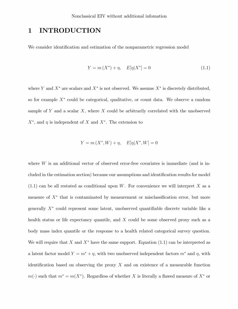
We consider identi�cation and estimation of the nonparametric regression model
Y = m (X�) + �; E[�jX�] = 0 (1.1)
where Y and X� are scalars and X� is not observed. We assume X� is discretely distributed,
so for example X� could be categorical, qualitative, or count data. We observe a random
sample of Y and a scalar X, where X could be arbitrarily correlated with the unobserved
X�, and � is independent of X and X�. The extension to
Y = m (X�;W ) + �; E[�jX�;W ] = 0
where W is an additional vector of observed error-free covariates is immediate (and is in-
cluded in the estimation section) because our assumptions and identi�cation results for model
(1.1) can be all restated as conditional upon W . For convenience we will interpret X as a
measure of X� that is contaminated by measurement or misclassi�cation error, but more
generally X� could represent some latent, unobserved quanti�able discrete variable like a
health status or life expectancy quantile, and X could be some observed proxy such as a
body mass index quantile or the response to a health related categorical survey question.
We will require that X and X� have the same support. Equation (1.1) can be interpreted as
a latent factor model Y = m�+ �, with two unobserved independent factors m� and �, with
identi�cation based on observing the proxy X and on existence of a measurable function
m(�) such that m� = m(X�). Regardless of whether X is literally a �awed measure of X� or
Nonclassical EIV without additional infomation
just some related covariate, we may still de�ne X �X� as a measurement error, though in
general this error will be nonclassical, that is, it will have nonzero mean not be independent
of X�.
Numerous data sets possess nonclassical measurement errors (see, e.g., Bound, Brown and
Mathiowetz (2001) for a review), however, to the best of our knowledge, there is no published
work that allows for nonparametric identi�cation and estimation of nonparametric regression
models with nonclassical measurement errors without parametric restrictions or additional
sample information such as instrumental variables, repeated measurements, or validation
data, which our paper provides. In short, we nonparametrically recover the conditional
density fY jX� (or equivalently, the function m and the density of �) just from the observed
joint distribution fY;X , while imposing minimal restrictions on the joint distribution fX;X�.
The relationship between the latent model fY jX� and the observed density fY;X is
fY;X(y; x) =
ZfY jX�(yjx�)fX;X� (x; x�) dx�: (1.2)
All the existing published papers for identifying the latent model fY jX� use one of the three
methods: i) assuming the measurement error structure fXjX� belongs to a parametric family
(see, e.g., Fuller (1987), Bickel and Ritov (1987), Hsiao (1991), Murphy and Van der Vaart
(1996), Wang, Lin, Gutierrez and Carroll (1998), Liang, Hardle and Carroll (1999), Taupin
(2001), Hong and Tamer (2003), Liang and Wang (2005)); ii) assuming there exists an ad-
ditional exogenous variable Z in the sample (such as an instrument or a repeated measure)
that does not enter the latent model fY jX�, and exploiting assumed restrictions on fY jX�;Z
and fX;X�;Z to identify fY jX� given the joint distribution of fy; x; zg (see, e.g., Hausman,
Nonclassical EIV without additional infomation
Ichimura, Newey and Powell (1991), Li and Vuong (1998), Li (2002), Wang (2004), Schen-
nach (2004), Carroll, Ruppert, Crainiceanu, Tosteson and Karagas (2004), Mahajan (2006),
Lewbel (2007), Hu (2006) and Hu and Schennach (2006)); or iii) assuming a secondary sam-
ple to provide information on fX;X� to permit recovery of fY jX� from the observed fY;X in
the primary sample (see, e.g., Carroll and Stefanski (1990), Lee and Sepanski (1995), Chen,
Hong, and Tamer (2005), Chen, Hong, and Tarozzi (2007), Hu and Ridder (2006)). Detailed
reviews on existing approaches and results can be found in several recent books and surveys
on measurement error models; see, e.g., Carroll, Ruppert, Stefanski and Crainiceanu (2006),
Chen, Hong and Nekipelov (2007), Bound, Brown and Mathiowetz (2001), Wansbeek and
Meijer (2000), and Cheng and Van Ness (1999).
In this paper, we obtain identi�cation by exploiting nonparametric features of the latent
model fY jX�, such as independence of the regression error term �. Our results are useful be-
cause many applications specify the latent model of interest fY jX�, while often little is known
about fXjX�, that is, about the nature of the measurement error or the exact relationship
between the unobserved latent X� and a proxy X. In addition, our key �rank�condition for
identi�cation is directly testable from the data.
Our identi�cation method is based on characteristic functions. Suppose X and X� have
support X = f1; 2; :::; Jg. Then by equation (1.1), exp (itY ) = exp (it�)PJ
j=1 1(X� =
j) exp [im (j) t] for any given constant t, where 1() is the indicator function that equals one if
its argument is true and zero otherwise. This equation and independence of � yield moments
E [exp (itY ) j X = x] = E [exp (it�)]JX
x�=1
fX�jX(x�jx) exp [im (x�) t] (1.3)
Nonclassical EIV without additional infomation
Evaluating equation (1.3) for t 2 ft1; :::; tKg and x 2 f1; 2; :::; Jg provides KJ equations in
J2 + J + K unknown constants. These unknown constants are the values of fX�jX(x�jx),
m (x�), and E [exp (it�)] for t 2 ft1; :::; tKg, x 2 f1; 2; :::; Jg, and x� 2 f1; 2; :::; Jg. Given a
large enough value of K, these moments provide more equations than unknowns. We provide
su¢ cient regularity assumption to ensure existence of some set of constants ft1; :::; tKg such
that these equations do not have multiple solutions, and the resulting unique solution to
these equations provides identi�cation of m() and of fX;X�, and hence of fY jX�.
As equation (1.3) shows, our identi�cation results depend on many moments of Y or
equivalently of �, rather than just on the conditional mean restrictionE[�jX�] = 0 that would
su¢ ce for identi�cation if X� were observed. Previous results, for example, Reiersol (1950),
Kendall and Stuart (1979), and Lewbel (1997), exist that obtain identi�cation based on
higher moments as we do (without instruments, repeated measures, or validation data), but
all these previous results have assumed either classical measurement error or/and parametric
restrictions.
Equation (1.3) implies that independence of the regression error � is actually stronger
than necessary for identi�cation, since e.g. we would obtain the same equations used for
identi�cation if we only had exp (it�) ? X�jX for t 2 ft1; :::; tKg. To illustrate this point
further, we provide an alternative identi�cation result for the dichotomous X� case without
the independence assumption, and in this case we can identify (solve) for all the unknowns
in closed-form.
Estimation could be based directly on equation (1.3) using, for example, Hansen�s (1982)
Generalized Method of Moments (GMM). However, this would require knowing or choos-
ing constants t1; :::; tK . Moreover, under the independence assumption of � and X�, we
Nonclassical EIV without additional infomation
have potentially in�nitely many constants t that solves equation (1.3); hence GMM esti-
mation using �nitely many such t�s will not be e¢ cient in general. One could apply the
in�nite-dimensional Z-estimation as described in Van der Vaart and Wellner (1996), here
we instead apply the method of sieve Maximum Likelihood (ML) of Grenander (1981) and
Geman and Hwang (1982), which does not require knowing or choosing constants t1; :::; tK ,
and easily allows for an additional vector of error-free covariatesW . The sieve ML estimator
essentially replaces the unknown functions f�, m, and fX�jX;W with polynomials, Fourier
series, splines, wavelets or other sieve approximators, and estimates the parameters of these
approximations by maximum likelihood. By simple applications of the general theory on
sieve MLE developed in Wong and Shen (1995), Shen (1997), Van de Geer (1993, 2000) and
others, we provide consistency and convergence rate of the sieve MLE, and root-n asymp-
totic normality and semiparametric e¢ ciency of smooth functionals of interest, such as the
weighted averaged derivatives of the latent nonparametric regression function m(X�;W ), or
the �nite-dimensional parameters (�) in a semiparametric speci�cation of m(X�;W ; �).
The rest of this paper is organized as follows. Section 2 provides the identi�cation results.
Section 3 describes the sieve ML estimator and presents its large sample properties. Section
4 provides two small simulation studies. Section 5 brie�y concludes and all the proofs are in
the appendix.
2 NONPARAMETRIC IDENTIFICATION
Our basic nonparametric regression model is equation (1.1) with scalar Y and X� 2 X =
f1; 2; :::; Jg. We observe a random sample of (X; Y ) 2 X �Y, where X is a proxy of X�. The
Nonclassical EIV without additional infomation
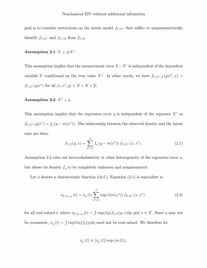
goal is to consider restrictions on the latent model fY jX� that su¢ ce to nonparametrically
identify fY jX� and fX�jX from fY jX .
Assumption 2.1 X ? �jX�.
This assumption implies that the measurement errorX�X� is independent of the dependent
variable Y conditional on the true value X�. In other words, we have fY jX�;X(yjx�; x) =
fY jX�(yjx�) for all (x; x�; y) 2 X � X � Y.
Assumption 2.2 X� ? �:
This assumption implies that the regression error � is independent of the regressor X� so
fY jX� (yjx�) = f� (y �m(x�)). The relationship between the observed density and the latent
ones are then:
fY;X(y; x) =JX
x�=1
f� (y �m(x�)) fX;X� (x; x�) : (2.1)
Assumption 2.2 rules out heteroskedasticity or other heterogeneity of the regression error �,
but allows its density f� to be completely unknown and nonparametric.
Let � denote a characteristic function (ch.f.). Equation (2.1) is equivalent to
�Y;X=x (t) = �� (t)JX
x�=1
exp (itm(x�)) fX;X� (x; x�) ; (2.2)
for all real-valued t, where �Y;X=x (t) =Rexp(ity)fY;X(y; x)dy and x 2 X . Since � may not
be symmetric, �� (t) =Rexp(it�)f�(�)d� need not be real-valued. We therefore let
�� (t) ����� (t)�� exp (ia (t)) ;
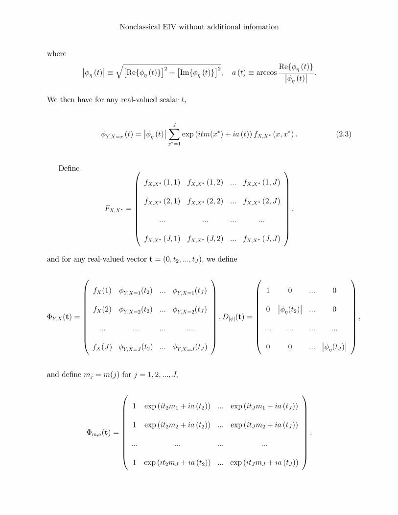
Nonclassical EIV without additional infomation
where ���� (t)�� �q�Ref�� (t)g�2 + �Imf�� (t)g�2; a (t) � arccosRef�� (t)g���� (t)�� :
We then have for any real-valued scalar t,
�Y;X=x (t) =���� (t)�� JX
x�=1
exp (itm(x�) + ia (t)) fX;X� (x; x�) : (2.3)
De�ne
FX;X� =
0BBBBBBBBBB@
fX;X� (1; 1) fX;X� (1; 2) ::: fX;X� (1; J)
fX;X� (2; 1) fX;X� (2; 2) ::: fX;X� (2; J)
::: ::: ::: :::
fX;X� (J; 1) fX;X� (J; 2) ::: fX;X� (J; J)
1CCCCCCCCCCA;
and for any real-valued vector t = (0; t2; :::; tJ), we de�ne
�Y;X(t) =
0BBBBBBBBBB@
fX(1) �Y;X=1(t2) ::: �Y;X=1(tJ)
fX(2) �Y;X=2(t2) ::: �Y;X=2(tJ)
::: ::: ::: :::
fX(J) �Y;X=J(t2) ::: �Y;X=J(tJ)
1CCCCCCCCCCA; Dj�j(t) =
0BBBBBBBBBB@
1 0 ::: 0
0����(t2)�� ::: 0
::: ::: ::: :::
0 0 :::����(tJ)��
1CCCCCCCCCCA;
and de�ne mj = m(j) for j = 1; 2; :::; J;
�m;a(t) =
0BBBBBBBBBB@
1 exp (it2m1 + ia (t2)) ::: exp (itJm1 + ia (tJ))
1 exp (it2m2 + ia (t2)) ::: exp (itJm2 + ia (tJ))
::: ::: ::: :::
1 exp (it2mJ + ia (t2)) ::: exp (itJmJ + ia (tJ))
1CCCCCCCCCCA:

Nonclassical EIV without additional infomation
With these matrix notations, for any real-valued vector t equation (2.3) is equivalent to
�Y;X(t) = FX;X� � �m;a(t)�Dj�j(t): (2.4)
Equation (2.4) relates the known parameters �Y;X(t) (which may be interpreted as re-
duced form parameters of the model) to the unknown structural parameters FX;X�, �m;a(t),
and Dj�j(t). Equation (2.4) provides a su¢ cient number of equality constraints to iden-
tify the structural parameters given the reduced form parameters, so what is required are
su¢ cient invertibility or rank restrictions to rule out multiple solutions of these equations.
To provide these conditions, consider both the real and imaginary parts of �Y;X(t). Since
Dj�j(t) is real by de�nition, we have
Ref�Y;X(t)g = FX;X� � Ref�m;a(t)g �Dj�j(t); (2.5)
and
Imf�Y;X(t)g = FX;X� � Imf�m;a(t)g �Dj�j(t): (2.6)
The matrices Imf�Y;X(t)g and Imf�m;a(t)g are not invertible because their �rst columns
are zeros, so we replace equation (2.6) with
(Imf�Y;X(t)g+�X) = FX;X� � (Imf�m;a(t)g+�)�Dj�j(t); (2.7)
Nonclassical EIV without additional infomation
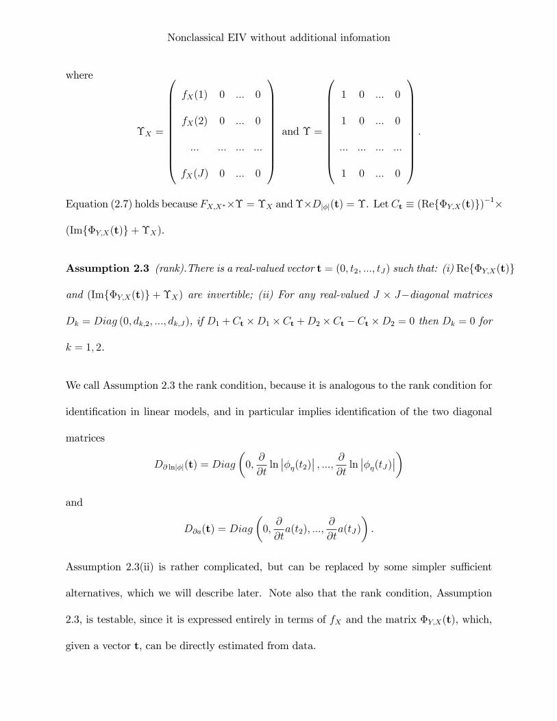
where
�X =
0BBBBBBBBBB@
fX(1) 0 ::: 0
fX(2) 0 ::: 0
::: ::: ::: :::
fX(J) 0 ::: 0
1CCCCCCCCCCAand � =
0BBBBBBBBBB@
1 0 ::: 0
1 0 ::: 0
::: ::: ::: :::
1 0 ::: 0
1CCCCCCCCCCA:
Equation (2.7) holds because FX;X��� = �X and��Dj�j(t) = �. LetCt � (Ref�Y;X(t)g)�1�
(Imf�Y;X(t)g+�X).
Assumption 2.3 (rank).There is a real-valued vector t = (0; t2; :::; tJ) such that: (i) Ref�Y;X(t)g
and (Imf�Y;X(t)g+�X) are invertible; (ii) For any real-valued J � J�diagonal matrices
Dk = Diag (0; dk;2; :::; dk;J), if D1 +Ct �D1 �Ct +D2 �Ct �Ct �D2 = 0 then Dk = 0 for
k = 1; 2.
We call Assumption 2.3 the rank condition, because it is analogous to the rank condition for
identi�cation in linear models, and in particular implies identi�cation of the two diagonal
matrices
D@ lnj�j(t) = Diag
�0;@
@tln����(t2)�� ; :::; @@t ln ����(tJ)��
�
and
D@a(t) = Diag
�0;@
@ta(t2); :::;
@
@ta(tJ)
�.
Assumption 2.3(ii) is rather complicated, but can be replaced by some simpler su¢ cient
alternatives, which we will describe later. Note also that the rank condition, Assumption
2.3, is testable, since it is expressed entirely in terms of fX and the matrix �Y;X(t), which,
given a vector t, can be directly estimated from data.
Nonclassical EIV without additional infomation
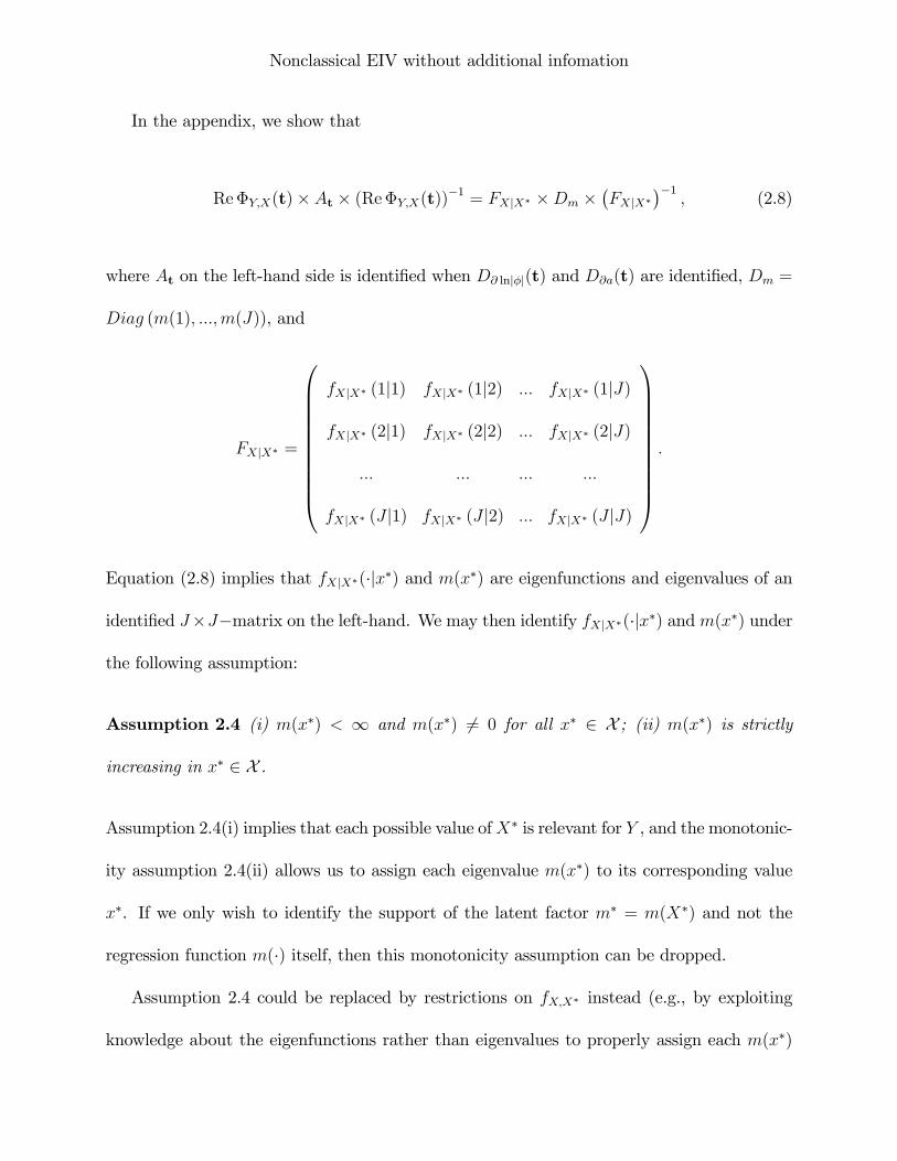
In the appendix, we show that
Re�Y;X(t)� At � (Re�Y;X(t))�1 = FXjX� �Dm ��FXjX�
��1; (2.8)
where At on the left-hand side is identi�ed when D@ lnj�j(t) and D@a(t) are identi�ed, Dm =
Diag (m(1); :::;m(J)), and
FXjX� =
0BBBBBBBBBB@
fXjX� (1j1) fXjX� (1j2) ::: fXjX� (1jJ)
fXjX� (2j1) fXjX� (2j2) ::: fXjX� (2jJ)
::: ::: ::: :::
fXjX� (J j1) fXjX� (J j2) ::: fXjX� (J jJ)
1CCCCCCCCCCA:
Equation (2.8) implies that fXjX�(�jx�) and m(x�) are eigenfunctions and eigenvalues of an
identi�ed J�J�matrix on the left-hand. We may then identify fXjX�(�jx�) andm(x�) under
the following assumption:
Assumption 2.4 (i) m(x�) < 1 and m(x�) 6= 0 for all x� 2 X ; (ii) m(x�) is strictly
increasing in x� 2 X .
Assumption 2.4(i) implies that each possible value ofX� is relevant for Y , and the monotonic-
ity assumption 2.4(ii) allows us to assign each eigenvalue m(x�) to its corresponding value
x�. If we only wish to identify the support of the latent factor m� = m(X�) and not the
regression function m(�) itself, then this monotonicity assumption can be dropped.
Assumption 2.4 could be replaced by restrictions on fX;X� instead (e.g., by exploiting
knowledge about the eigenfunctions rather than eigenvalues to properly assign each m(x�)
Nonclassical EIV without additional infomation
to its corresponding value x�), but assumption 2.4 is more in line with our other assumptions,
which assume that we have information about our regression model but know very little about
the relationship of the unobserved X� to the proxy X.
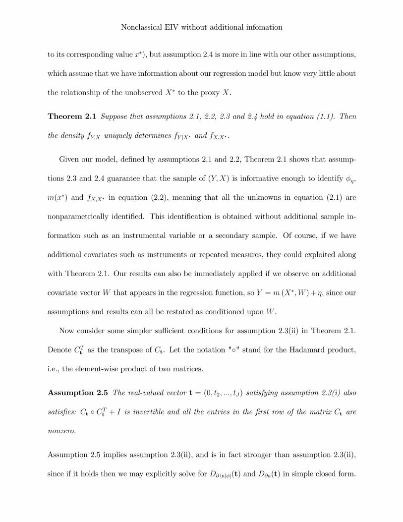
Theorem 2.1 Suppose that assumptions 2.1, 2.2, 2.3 and 2.4 hold in equation (1.1). Then
the density fY;X uniquely determines fY jX� and fX;X�.
Given our model, de�ned by assumptions 2.1 and 2.2, Theorem 2.1 shows that assump-
tions 2.3 and 2.4 guarantee that the sample of (Y;X) is informative enough to identify ��,
m(x�) and fX;X� in equation (2.2), meaning that all the unknowns in equation (2.1) are
nonparametrically identi�ed. This identi�cation is obtained without additional sample in-
formation such as an instrumental variable or a secondary sample. Of course, if we have
additional covariates such as instruments or repeated measures, they could exploited along
with Theorem 2.1. Our results can also be immediately applied if we observe an additional
covariate vector W that appears in the regression function, so Y = m (X�;W )+ �, since our
assumptions and results can all be restated as conditioned upon W .
Now consider some simpler su¢ cient conditions for assumption 2.3(ii) in Theorem 2.1.
Denote CTt as the transpose of Ct. Let the notation "�" stand for the Hadamard product,
i.e., the element-wise product of two matrices.
Assumption 2.5 The real-valued vector t = (0; t2; :::; tJ) satisfying assumption 2.3(i) also
satis�es: Ct � CTt + I is invertible and all the entries in the �rst row of the matrix Ct are
nonzero.
Assumption 2.5 implies assumption 2.3(ii), and is in fact stronger than assumption 2.3(ii),
since if it holds then we may explicitly solve for D@ lnj�j(t) and D@a(t) in simple closed form.
Nonclassical EIV without additional infomation
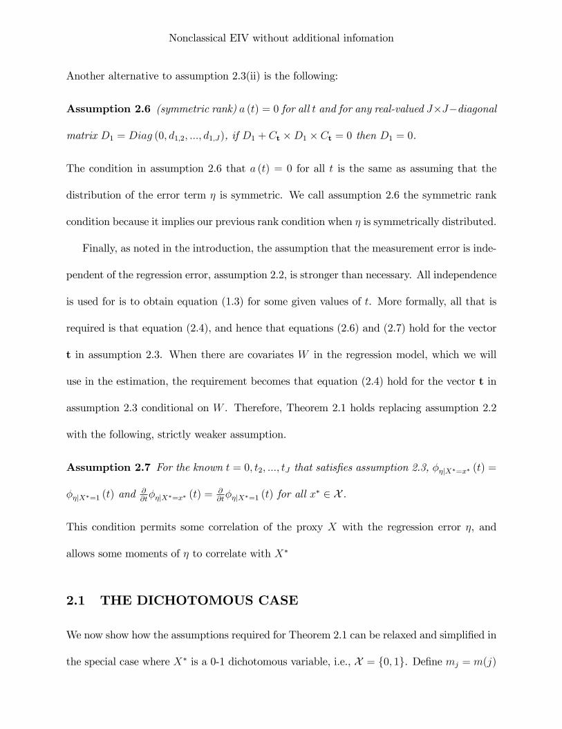
Another alternative to assumption 2.3(ii) is the following:
Assumption 2.6 (symmetric rank) a (t) = 0 for all t and for any real-valued J�J�diagonal
matrix D1 = Diag (0; d1;2; :::; d1;J), if D1 + Ct �D1 � Ct = 0 then D1 = 0.
The condition in assumption 2.6 that a (t) = 0 for all t is the same as assuming that the
distribution of the error term � is symmetric. We call assumption 2.6 the symmetric rank
condition because it implies our previous rank condition when � is symmetrically distributed.
Finally, as noted in the introduction, the assumption that the measurement error is inde-
pendent of the regression error, assumption 2.2, is stronger than necessary. All independence
is used for is to obtain equation (1.3) for some given values of t. More formally, all that is
required is that equation (2.4), and hence that equations (2.6) and (2.7) hold for the vector
t in assumption 2.3. When there are covariates W in the regression model, which we will
use in the estimation, the requirement becomes that equation (2.4) hold for the vector t in
assumption 2.3 conditional on W . Therefore, Theorem 2.1 holds replacing assumption 2.2
with the following, strictly weaker assumption.
Assumption 2.7 For the known t = 0; t2; :::; tJ that satis�es assumption 2.3, ��jX�=x� (t) =
��jX�=1 (t) and@@t��jX�=x� (t) =
@@t��jX�=1 (t) for all x
� 2 X .
This condition permits some correlation of the proxy X with the regression error �, and
allows some moments of � to correlate with X�
2.1 THE DICHOTOMOUS CASE
We now show how the assumptions required for Theorem 2.1 can be relaxed and simpli�ed in
the special case where X� is a 0-1 dichotomous variable, i.e., X = f0; 1g. De�ne mj = m(j)
Nonclassical EIV without additional infomation
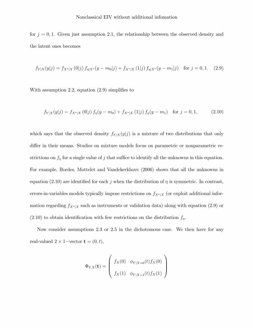
for j = 0; 1. Given just assumption 2.1, the relationship between the observed density and
the latent ones becomes
fY jX(yjj) = fX�jX (0jj) f�jX�(y �m0jj) + fX�jX (1jj) f�jX�(y �m1jj) for j = 0; 1: (2.9)
With assumption 2.2, equation (2.9) simpli�es to
fY jX(yjj) = fX�jX (0jj) f�(y �m0) + fX�jX (1jj) f�(y �m1) for j = 0; 1; (2.10)
which says that the observed density fY jX(yjj) is a mixture of two distributions that only
di¤er in their means. Studies on mixture models focus on parametric or nonparametric re-
strictions on f� for a single value of j that su¢ ce to identify all the unknowns in this equation.
For example, Bordes, Mottelet and Vandekerkhove (2006) shows that all the unknowns in
equation (2.10) are identi�ed for each j when the distribution of � is symmetric. In contrast,
errors-in-variables models typically impose restrictions on fX�jX (or exploit additional infor-
mation regarding fX�jX such as instruments or validation data) along with equation (2.9) or
(2.10) to obtain identi�cation with few restrictions on the distribution f�.
Now consider assumptions 2.3 or 2.5 in the dichotomous case. We then have for any
real-valued 2� 1�vector t = (0; t),
�Y;X(t) =
0BB@ fX(0) �Y jX=0(t)fX(0)
fX(1) �Y jX=1(t)fX(1)
1CCA
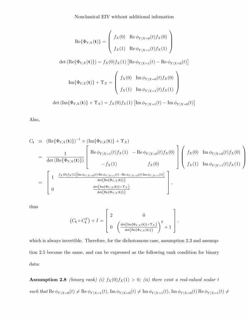
Nonclassical EIV without additional infomation
Ref�Y;X(t)g =
0BB@ fX(0) Re�Y jX=0(t)fX(0)
fX(1) Re�Y jX=1(t)fX(1)
1CCAdet (Ref�Y;X(t)g) = fX(0)fX(1)
�Re�Y jX=1(t)� Re�Y jX=0(t)
�
Imf�Y;X(t)g+�X =
0BB@ fX(0) Im�Y jX=0(t)fX(0)
fX(1) Im�Y jX=1(t)fX(1)
1CCAdet (Imf�Y;X(t)g+�X) = fX(0)fX(1)
�Im�Y jX=1(t)� Im�Y jX=0(t)
�Also,
Ct � (Ref�Y;X(t)g)�1 � (Imf�Y;X(t)g+�X)
=1
det (Ref�Y;X(t)g)
2664 Re�Y jX=1(t)fX(1) �Re�Y jX=0(t)fX(0)
�fX(1) fX(0)
37750BB@ fX(0) Im�Y jX=0(t)fX(0)
fX(1) Im�Y jX=1(t)fX(1)
1CCA
=
2664 1fX(0)fX(1)[Im�Y jX=0(t)Re�Y jX=1(t)�Re�Y jX=0(t) Im�Y jX=1(t)]
det(Ref�Y;X(t)g)
0det(Imf�Y;X(t)g+�X)det(Ref�Y;X(t)g)
3775 ;
thus
�Ct � CTt
�+ I =
2664 2 0
0
�det(Imf�Y;X(t)g+�X)det(Ref�Y;X(t)g)
�2+ 1
3775 ;which is always invertible. Therefore, for the dichotomous case, assumption 2.3 and assump-
tion 2.5 become the same, and can be expressed as the following rank condition for binary
data:
Assumption 2.8 (binary rank) (i) fX(0)fX(1) > 0; (ii) there exist a real-valued scalar t
such that Re�Y jX=0(t) 6= Re�Y jX=1(t), Im�Y jX=0(t) 6= Im�Y jX=1(t), Im�Y jX=0(t) Re�Y jX=1(t) 6=
Nonclassical EIV without additional infomation
Re�Y jX=0(t) Im�Y jX=1(t).
It should be generally easy to �nd a real-valued scalar t that satis�es this binary rank
condition.
In the dichotomous case, instead of imposing Assumption 2.4, we may obtain the ordering
of mj from that of observed �j � E(Y jX = j) under the following assumption:
Assumption 2.9 (i) �1 > �0; (ii) fX�jX (1j0) + fX�jX (0j1) < 1:
Assumption 2.9(i) is not restrictive because one can always rede�ne X as 1 �X if needed.
Assumption 2.9(ii) reveals the ordering of m1 and m0, by making it the same as that of �1
and �0 because
1� fX�jX (1j0)� fX�jX (0j1) =�1 � �0m1 �m0
;
so m1 � �1 > �0 � m0. Assumption 2.9(ii) says that the sum of misclassi�cation prob-
abilities is less than one, meaning that, on average, the observations X are more accurate
predictions of X� than pure guesses. See Lewbel (2007) for further discussion of this as-
sumption.
The following Corollary is a direct application of Theorem 2.1; hence we omit its proof.
Corollary 2.2 Suppose that X = f0; 1g, equations (1.1) and (2.10), assumptions 2.8 and
2.9 hold. Then the density fY;X uniquely determines fY jX� and fX;X�.
2.1.1 IDENTIFICATION WITHOUT INDEPENDENCE
We now show how to obtain identi�cation in the dichotomous case without the independent
regression error assumption 2.2. Given just assumption 2.1, Equation (2.9) implies that
Nonclassical EIV without additional infomation
the observed density fY jX(yjj) is a mixture of two conditional densities f�jX�(y �m0jj) and
f�jX�(y �m1jj).
Instead of assuming the independence between X� and �, we impose the following weaker
assumption:
Assumption 2.10 E��kjX�� = E ��k� for k = 2; 3.
Only these two moment restrictions are needed because we only need to solve for two un-
knowns, m0 and m1. Identi�cation could also be obtained using other, similar restrictions
such as quantiles or modes. For example, one of the moments in this assumption 2.10 might
be replaced with assuming that the density f�jX�=0 has zero median. Equation (2.9) then
implies that
0:5 =�1 �m0
�1 � �0
Z m0
�1fY jX=0(y)dy +
m0 � �0�1 � �0
Z m0
�1fY jX=1(y)dy
which may uniquely identifym0 under some testable assumptions. An advantage of Assump-
tion 2.10 is that we obtain a closed-form solution for m0 and m1.
De�ne vj � Eh�Y � �j
�2 jX = ji, sj � E
h�Y � �j
�3 jX = ji,
C1 �(v1 + �
21)� (v0 + �20)�1 � �0
; C2 �1
2(�1 � �0)
2 +3
2
�v1 � v0�1 � �0
�2� s1 � s0�1 � �0
:
We leave the detailed proof to the appendix and present the result as follows:
Theorem 2.3 Suppose that X = f0; 1g, equations (1.1) and (2.9), assumptions 2.9 and
2.10 hold. Then the density fY jX uniquely determines fY jX� and fX�jX . To be speci�c, we
Nonclassical EIV without additional infomation
have
m0 =1
2C1 �
r1
2C2; m1 =
1
2C1 +
r1
2C2;
fX�jX (1j0) =�0 � 1
2C1p
2C2� 12; fX�jX (0j1) =
12C1 � �1p2C2
� 12;
and
fY jX�=j(y) =�1 �mj
�1 � �0fY jX=0(y) +
mj � �0�1 � �0
fY jX=1(y):
3 SIEVE MAXIMUM LIKELIHOOD ESTIMATION
This section considers the estimation of a nonparametric regression model as follows:
Y = m0 (X�;W ) + �;
where the function m0() is unknown and W is a vector of error-free covariates and �
is independent of (X�;W ). Let fZt � (Yt; Xt;Wt)gnt=1 denote a random sample of Z �
(Y;X;W ). We have shown that fY jX�;W and fX�jX;W are identi�ed from fY jX;W . Let
�0 � (f01; f02; f03)T �
�f�; fX�jX;W ;m0
�Tbe the true parameters of interest. Then the
observed likelihood of Y given (X;W ) (or the likelihood for �0) is
nYt=1
fY jX;W (YtjXt;Wt) =
nYt=1
(Xx�2X
f� (Yt �m0(x�;Wt)) fX�jX;W (x
�jXt;Wt)
):
Before we present a sieve ML estimator b� for �0, we need to impose some mild smoothnessrestrictions on the unknown functions �0 �
�f�; fX�jX;W ;m0
�T. The sieve method allows for
Nonclassical EIV without additional infomation
unknown functions belonging to many di¤erent function spaces such as Sobolev space, Besov
space and others; see e.g., Shen and Wong (1994), Wong and Shen (1995), Shen (1997) and
Van de Geer (1993, 2000). But, for the sake of concreteness and simplicity, we consider the
widely used Hölder space of functions. Let � = (�1; :::; �d)T 2 Rd, a = (a1; :::; ad)
T be a
vector of non-negative integers, and
rah(�) � @jaj
@�a11 � � � @�add
h(�1; :::; �d)
denote the jaj = a1 + � � � + ad -th derivative. Let k�kE denote the Euclidean norm. Let
V � Rd and be the largest integer satisfying > . The Hölder space � (V) of order
> 0 is a space of functions h : V 7! R such that the �rst derivatives are continuous and
bounded, and the -th derivative are Hölder continuous with the exponent � 2 (0; 1].
The Hölder space � (V) becomes a Banach space under the Hölder norm:
khk� = maxjaj� sup�jrah(�)j+max
jaj= sup� 6=�0
jrah(�)�rah(�0)j(k� � �0kE)
� <1:
Denote � c (V) � fh 2 � (V) : khk� � c <1g as a Hölder ball. Let � 2 R, W 2 W with
W a compact convex subset in Rdw . Also denote
F1 =�p
f1(�) 2 � 1c (R) : f1(�) > 0,ZRf1(�)d� = 1
�;
F2 =�p
f2 (x�jx; �) 2 � 2c (W) : f2 (�j�; �) > 0,ZXf2 (x
�jx;w) dx� = 1 for all x 2 X , w 2 W�;
Nonclassical EIV without additional infomation
and
F3 = ff3 (x�; �) 2 � 3c (W) : f3 (i; w) > f3 (j; w) for all i > j, i; j 2 X , w 2 Wg
We impose the following smoothness restrictions on the densities:
Assumption 3.1 (i) all the assumptions in Theorem 2.1 hold; (ii) f�(�) 2 F1 with 1 > 1=2;
(iii) fX�jX;W (x�jx; �) 2 F2 with 2 > dw=2 for all x�; x 2 X � f1; :::; Jg; (iv) m0(x
�; �) 2 F3
with 3 > dw=2 for all x� 2 X :
Denote A = F1 � F2 � F3 and � = (f1; f2; f3)T . Let E[�] denote the expectation with
respect to the underlying true data generating process for Zt. Then �0 � (f01; f02; f03)T =
argmax�2AE[`(Zt;�)], where
`(Zt;�) � ln(Xx�2X
f1 (Yt � f3(x�;Wt)) f2 (x�jXt;Wt)
): (3.1)
Let An = Fn1 �Fn
2 �Fn3 be a sieve space for A, which is a sequence of approximating spaces
that are dense in A under some pseudo-metric. The sieve MLE b�n = � bf1; bf2; bf3�T 2 An for�0 2 A is de�ned as:
b�n = argmax�2An
nXt=1
`(Zt;�): (3.2)
We could apply in�nite-dimensional approximating spaces as sieves Fnj for Fj; j = 1; 2; 3.
However, in applications, we shall use �nite-dimensional sieve spaces since they are easier to
implement. For j = 1; 2; 3, let pkj;nj (�) be a kj;n� 1�vector of known basis functions, such as
power series, splines, Fourier series, etc. Then we denote the sieve space for Fj; j = 1; 2; 3
Nonclassical EIV without additional infomation
as follows:
Fn1 =
npf1(�) = pk1;n1 (�)T�1 2 F1
o;
Fn2 =
(pf2 (x�jx; �) =
JXk=1
JXj=1
I (x� = k) I (x = j) pk2;n2 (�)T�2;kj 2 F2
);
Fn3 =
(f3 (x
�; �) =JXk=1
I (x� = k) pk2;n3 (�)T�3;k 2 F3
):
We note that the method of sieve MLE is very �exible and we can easily impose prior
information on the parameter space (A) and the sieve space (An). For example, if the func-
tional form of the true regression function m0(x�; w) is known upto some �nite-dimensional
parameters �0 2 B, where B is a compact subset of Rd� , then we can take A = F1�F2�FB
and An = Fn1 � Fn
2 � FB with FB = ff3 (x�; w) = m0(x�; w; �) : � 2 Bg. The sieve MLE
becomes
b�n = argmax�2An
nXt=1
`(Zt;�); with `(Zt;�) = ln
(Xx�2X
f1 (Yt �m0(x�;Wt; �)) f2 (x
�jXt;Wt)
):
(3.3)
3.1 Consistency
The consistency of the sieve MLE b�n can be established by applying either Geman andHwang (1982) or lemma A.1 of Newey and Powell (2003). First we de�ne a norm on A as
follows:
k�ks = sup�
���h(�) �1 + �2���=2���+ supx�;x;w
jf2 (x�jx;w)j+ supx�;w
jf3 (x�; w)j for some � > 0:
Nonclassical EIV without additional infomation
We assume
Assumption 3.2 (i) �1 < E [`(Zt;�0)] < 1, E [`(Zt;�)] is upper semicontinuous on
A under the metric k�ks; (ii) there are a �nite � > 0 and a random variable U(Zt) with
EfU(Zt)g <1 such that sup�2An:k���0ks�� j`(Zt;�)� `(Zt;�0)j � ��U(Zt).
Assumption 3.3 (i) pk1;n1 (�) is a k1;n�1�vector of spline wavelet basis functions on R, and
for j = 2; 3, pkj;nj (�) is a kj;n � 1�vector of tensor product of spline basis functions on W;
(ii) kn � maxfk1;n; k2;n; k3;ng ! 1 and kn=n! 0.
The following consistency lemma is a direct application of lemma A.1 of Newey and
Powell (2003) or theorem 3.1 (or remark 3.1(4), remark 3.3) of Chen (2006); hence we omit
its proof.
Lemma 3.1 Let b�n be the sieve MLE. Under assumptions 3.1-3.3, we have kb�n � �0ks =op(1).
3.2 Convergence rate under the Fisher metric
Given Lemma 3.1, we can now restrict our attention to a shrinking jj � jjs�neighborhood
around �0. Let A0s � f� 2 A : jj� � �0jjs = o(1); jj�jjs � c0 < cg and A0sn � f� 2 An :
jj�� �0jjs = o(1); jj�jjs � c0 < cg. Then, for the purpose of establishing a convergence rate
under a pseudo metric that is weaker than jj � jjs, we can treat A0s as the new parameter
space and A0sn as its sieve space, and assume that both A0s and A0sn are convex parameter
spaces. For any �1, �2 2 A0s, we consider a continuous path f� (�) : � 2 [0; 1]g in A0s such
that � (0) = �1 and � (1) = �2. For simplicity we assume that for any �; � + v 2 A0s,
Nonclassical EIV without additional infomation
f�+ �v : � 2 [0; 1]g is a continuous path in A0s, and that `(Zt;�+ �v) is twice continuously
di¤erentiable at � = 0 for almost all Zt and any direction v 2 A0s. De�ne the pathwise �rst
derivative as
d`(Zt;�)
d�[v] � d`(Zt;�+ �v)
d�j�=0 a.s. Zt;
and the pathwise second derivative as
d2`(Zt;�)
d�d�T[v; v] � d2`(Zt;�+ �v)
d� 2j�=0 a.s. Zt:
De�ne the Fisher metric k�k on A0s as follows: for any �1, �2 2 A0s,
k�1 � �2k2 � E(�
d`(Zt;�0)
d�[�1 � �2]
�2):
We show that b�n converges to �0 at a rate faster than n�1=4 under the Fisher metric k�kwith the following assumptions:
Assumption 3.4 (i) � > 1; (ii) � minf 1; 2=dw; 3=dwg > 1=2:
Assumption 3.5 (i) A0s is convex at �0; (ii) `(Zt;�) is twice continuously pathwise di¤er-
entiable with respect to � 2 A0s.
Assumption 3.6 supe�2A0s sup�2A0sn���d`(Zt;e�)d�
h���0
k���0ks
i��� � U(Zt) for a random variable U(Zt)with Ef[U(Zt)]2g <1.
Nonclassical EIV without additional infomation
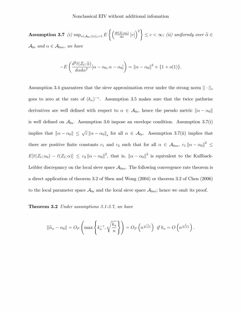
Assumption 3.7 (i) supv2A0s:jjvjjs=1E��
d`(Zt;�0)d�
[v]�2�
� c <1; (ii) uniformly over e� 2A0s and � 2 A0sn, we have
�E�d2`(Zt; e�)d�d�T
[�� �0; �� �0]�= k�� �0k2 � f1 + o(1)g:
Assumption 3.4 guarantees that the sieve approximation error under the strong norm jj � jjs
goes to zero at the rate of (kn)� . Assumption 3.5 makes sure that the twice pathwise
derivatives are well de�ned with respect to � 2 A0s, hence the pseudo metric k�� �0k
is well de�ned on A0s. Assumption 3.6 impose an envelope condition. Assumption 3.7(i)
implies that k�� �0k �pc k�� �0ks for all � 2 A0s. Assumption 3.7(ii) implies that
there are positive �nite constants c1 and c2 such that for all � 2 A0sn, c1 k�� �0k2 �
E[`(Zt;�0) � `(Zt;�)] � c2 k�� �0k2, that is, k�� �0k2 is equivalent to the Kullback-
Leibler discrepancy on the local sieve space A0sn. The following convergence rate theorem is
a direct application of theorem 3.2 of Shen and Wong (2004) or theorem 3.2 of Chen (2006)
to the local parameter space A0s and the local sieve space A0sn; hence we omit its proof.
Theorem 3.2 Under assumptions 3.1-3.7, we have
kb�n � �0k = OP max(k� n ;rknn)!
= OP
�n
� 2 +1
�if kn = O
�n
12 +1
�:
Nonclassical EIV without additional infomation
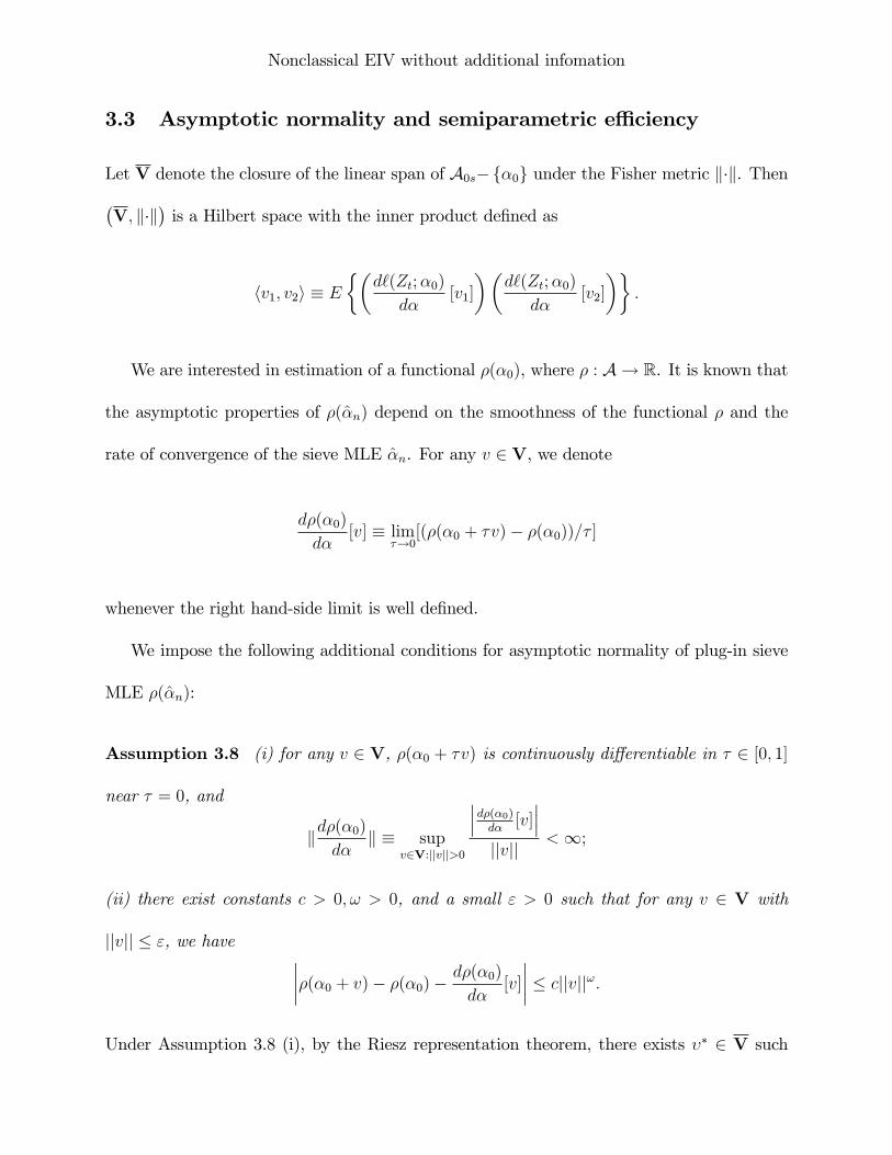
3.3 Asymptotic normality and semiparametric e¢ ciency
Let V denote the closure of the linear span of A0s�f�0g under the Fisher metric k�k. Then�V; k�k
�is a Hilbert space with the inner product de�ned as
hv1; v2i � E��
d`(Zt;�0)
d�[v1]
��d`(Zt;�0)
d�[v2]
��:
We are interested in estimation of a functional �(�0), where � : A ! R. It is known that
the asymptotic properties of �(�̂n) depend on the smoothness of the functional � and the
rate of convergence of the sieve MLE �̂n. For any v 2 V, we denote
d�(�0)
d�[v] � lim
�!0[(�(�0 + �v)� �(�0))=� ]
whenever the right hand-side limit is well de�ned.
We impose the following additional conditions for asymptotic normality of plug-in sieve
MLE �(�̂n):
Assumption 3.8 (i) for any v 2 V, �(�0 + �v) is continuously di¤erentiable in � 2 [0; 1]
near � = 0, and
kd�(�0)d�
k � supv2V:jjvjj>0
���d�(�0)d�[v]���
jjvjj <1;
(ii) there exist constants c > 0; ! > 0, and a small " > 0 such that for any v 2 V with
jjvjj � ", we have �����(�0 + v)� �(�0)� d�(�0)d�[v]
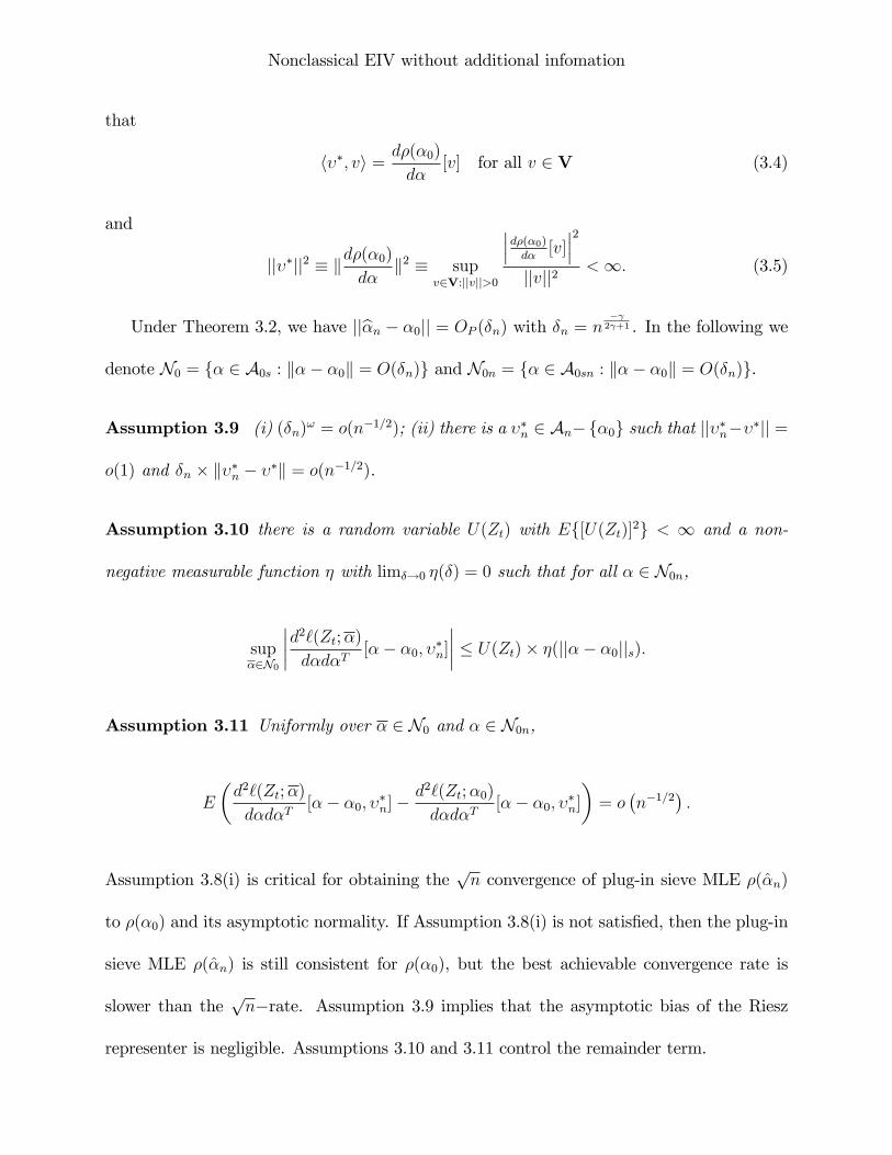
���� � cjjvjj!:Under Assumption 3.8 (i), by the Riesz representation theorem, there exists �� 2 V such
Nonclassical EIV without additional infomation
that
h��; vi = d�(�0)
d�[v] for all v 2 V (3.4)
and
jj��jj2 � kd�(�0)d�
k2 � supv2V:jjvjj>0
���d�(�0)d�[v]���2
jjvjj2 <1: (3.5)
Under Theorem 3.2, we have jjb�n � �0jj = OP (�n) with �n = n � 2 +1 . In the following we
denote N0 = f� 2 A0s : k�� �0k = O(�n)g and N0n = f� 2 A0sn : k�� �0k = O(�n)g.
Assumption 3.9 (i) (�n)! = o(n�1=2); (ii) there is a ��n 2 An�f�0g such that jj��n���jj =
o(1) and �n � k��n � ��k = o(n�1=2).
Assumption 3.10 there is a random variable U(Zt) with Ef[U(Zt)]2g < 1 and a non-
negative measurable function � with lim�!0 �(�) = 0 such that for all � 2 N0n,
sup�2N0
����d2`(Zt;�)d�d�T[�� �0; ��n]
���� � U(Zt)� �(jj�� �0jjs):Assumption 3.11 Uniformly over � 2 N0 and � 2 N0n,
E
�d2`(Zt;�)
d�d�T[�� �0; ��n]�
d2`(Zt;�0)
d�d�T[�� �0; ��n]
�= o
�n�1=2
�:
Assumption 3.8(i) is critical for obtaining thepn convergence of plug-in sieve MLE �(�̂n)
to �(�0) and its asymptotic normality. If Assumption 3.8(i) is not satis�ed, then the plug-in
sieve MLE �(�̂n) is still consistent for �(�0), but the best achievable convergence rate is
slower than thepn�rate. Assumption 3.9 implies that the asymptotic bias of the Riesz
representer is negligible. Assumptions 3.10 and 3.11 control the remainder term.
Nonclassical EIV without additional infomation
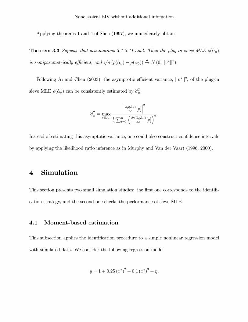
Applying theorems 1 and 4 of Shen (1997), we immediately obtain
Theorem 3.3 Suppose that assumptions 3.1-3.11 hold. Then the plug-in sieve MLE �(�̂n)
is semiparametrically e¢ cient, andpn (�(�̂n)� �(�0))
d! N (0; jj��jj2).
Following Ai and Chen (2003), the asymptotic e¢ cient variance, jj��jj2, of the plug-in
sieve MLE �(�̂n) can be consistently estimated by b�2n:
b�2n = maxv2An
���d�(b�n)d�[v]���2
1n
Pnt=1
�d`(Zt;b�n)
d�[v]�2 :
Instead of estimating this asymptotic variance, one could also construct con�dence intervals
by applying the likelihood ratio inference as in Murphy and Van der Vaart (1996, 2000).
4 Simulation
This section presents two small simulation studies: the �rst one corresponds to the identi�-
cation strategy, and the second one checks the performance of sieve MLE.
4.1 Moment-based estimation
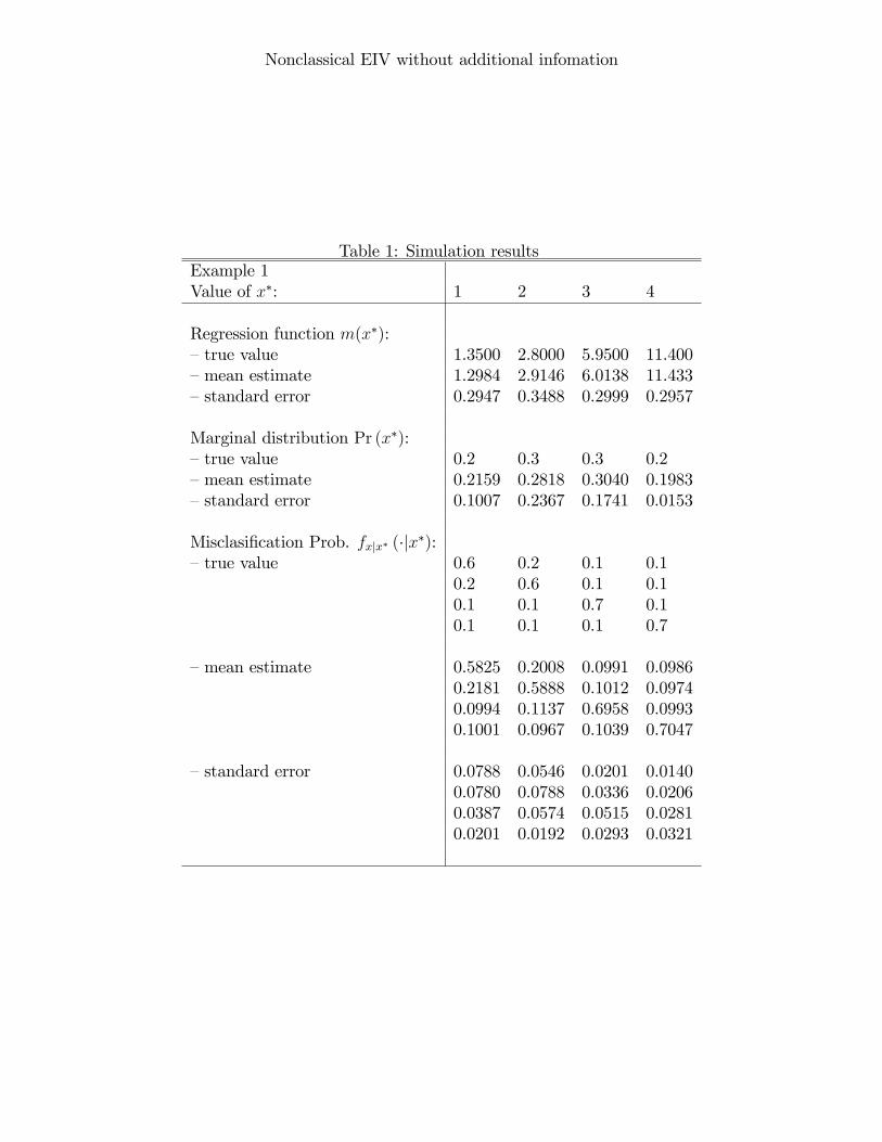
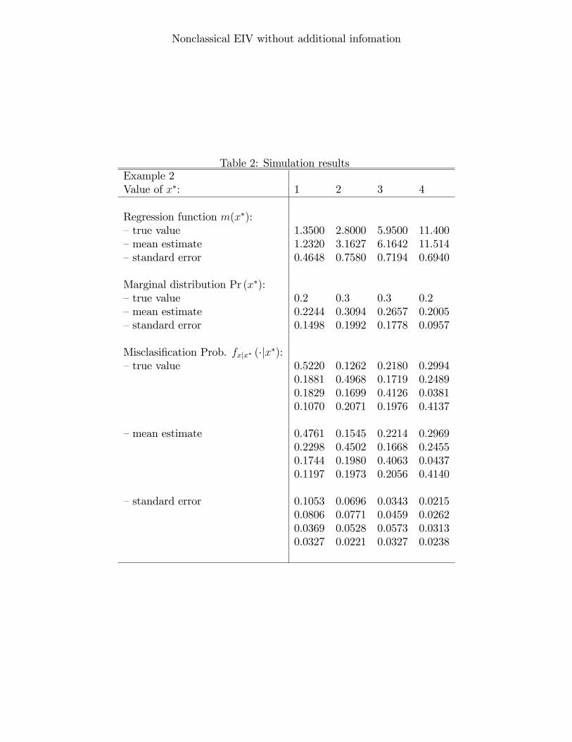
This subsection applies the identi�cation procedure to a simple nonlinear regression model
with simulated data. We consider the following regression model
y = 1 + 0:25 (x�)2 + 0:1 (x�)3 + �;
Nonclassical EIV without additional infomation
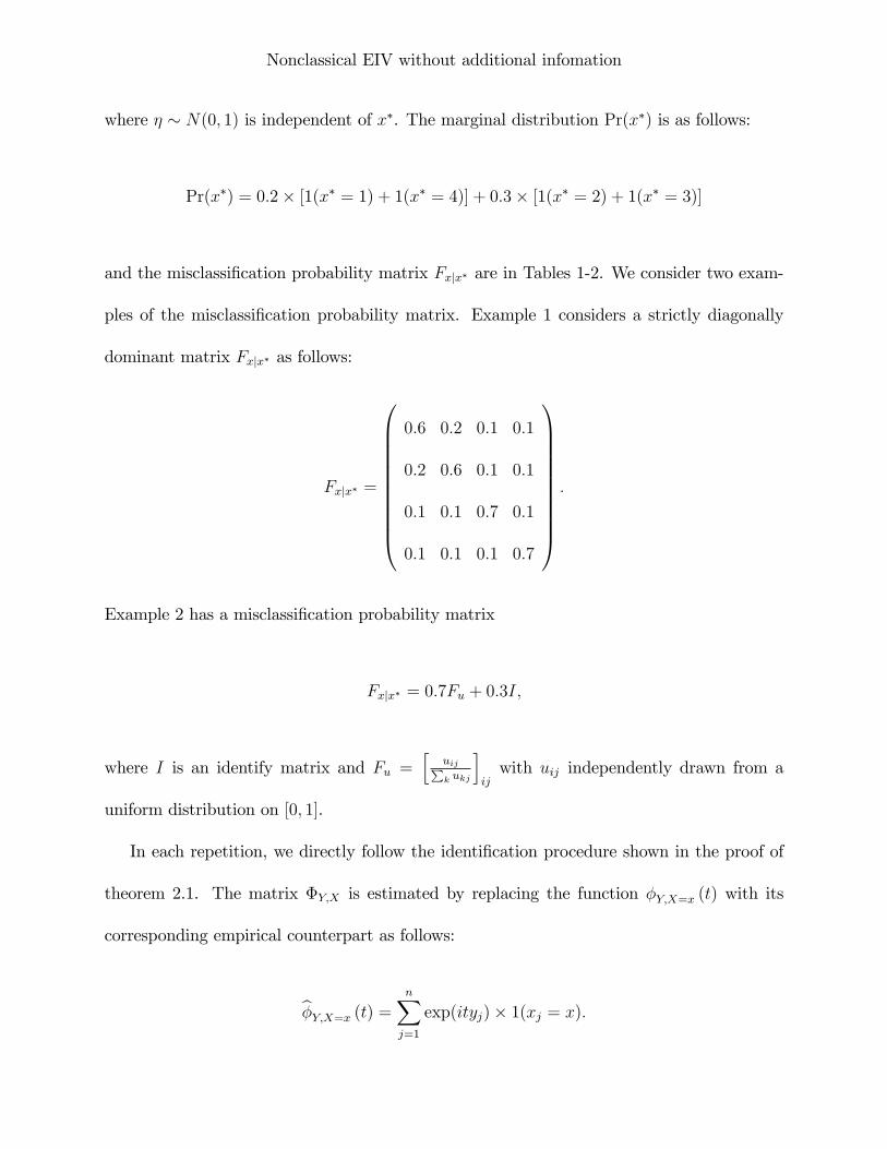
where � � N(0; 1) is independent of x�. The marginal distribution Pr(x�) is as follows:
Pr(x�) = 0:2� [1(x� = 1) + 1(x� = 4)] + 0:3� [1(x� = 2) + 1(x� = 3)]
and the misclassi�cation probability matrix Fxjx� are in Tables 1-2. We consider two exam-
ples of the misclassi�cation probability matrix. Example 1 considers a strictly diagonally
dominant matrix Fxjx� as follows:
Fxjx� =
0BBBBBBBBBB@
0:6 0:2 0:1 0:1
0:2 0:6 0:1 0:1
0:1 0:1 0:7 0:1
0:1 0:1 0:1 0:7
1CCCCCCCCCCA:
Example 2 has a misclassi�cation probability matrix
Fxjx� = 0:7Fu + 0:3I;
where I is an identify matrix and Fu =h
uijPk ukj
iijwith uij independently drawn from a
uniform distribution on [0; 1].
In each repetition, we directly follow the identi�cation procedure shown in the proof of
theorem 2.1. The matrix �Y;X is estimated by replacing the function �Y;X=x (t) with its
corresponding empirical counterpart as follows:
b�Y;X=x (t) = nXj=1
exp(ityj)� 1(xj = x):
Nonclassical EIV without additional infomation
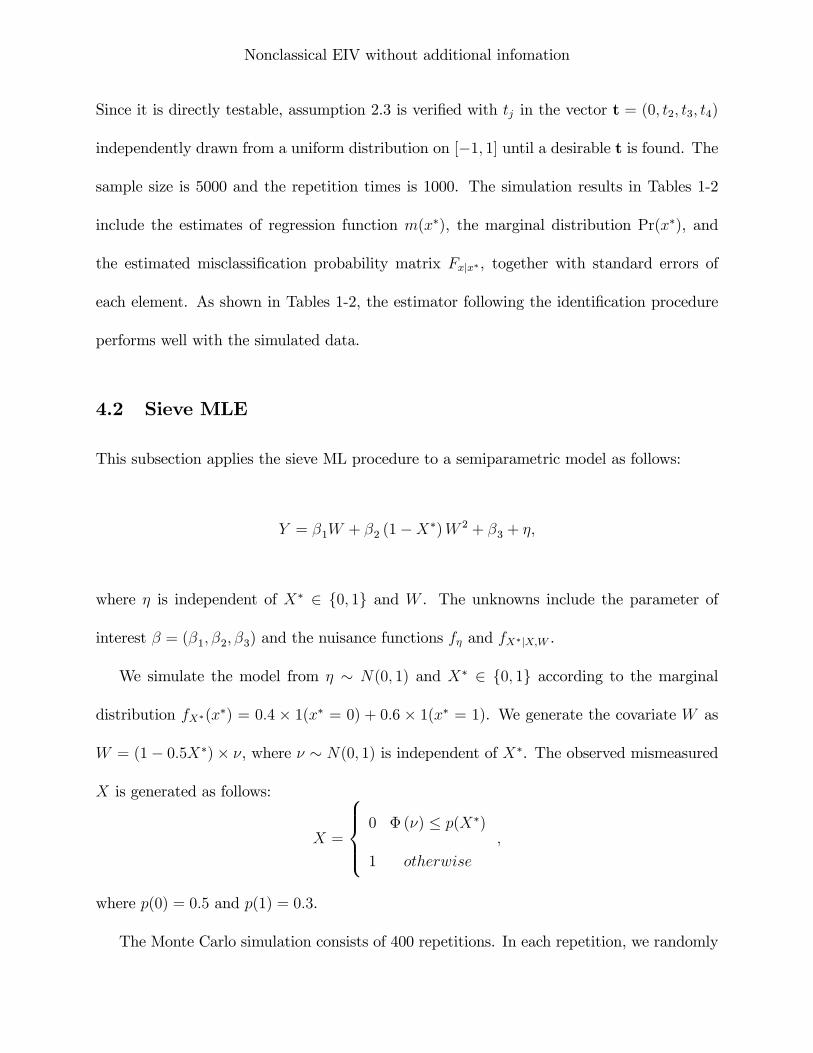
Since it is directly testable, assumption 2.3 is veri�ed with tj in the vector t = (0; t2; t3; t4)
independently drawn from a uniform distribution on [�1; 1] until a desirable t is found. The
sample size is 5000 and the repetition times is 1000. The simulation results in Tables 1-2
include the estimates of regression function m(x�), the marginal distribution Pr(x�), and
the estimated misclassi�cation probability matrix Fxjx�, together with standard errors of
each element. As shown in Tables 1-2, the estimator following the identi�cation procedure
performs well with the simulated data.
4.2 Sieve MLE
This subsection applies the sieve ML procedure to a semiparametric model as follows:
Y = �1W + �2 (1�X�)W 2 + �3 + �;
where � is independent of X� 2 f0; 1g and W . The unknowns include the parameter of
interest � = (�1; �2; �3) and the nuisance functions f� and fX�jX;W .
We simulate the model from � � N(0; 1) and X� 2 f0; 1g according to the marginal
distribution fX�(x�) = 0:4 � 1(x� = 0) + 0:6 � 1(x� = 1). We generate the covariate W as
W = (1� 0:5X�)� �, where � � N(0; 1) is independent of X�. The observed mismeasured
X is generated as follows:
X =
8>><>>:0 � (�) � p(X�)
1 otherwise
;
where p(0) = 0:5 and p(1) = 0:3.
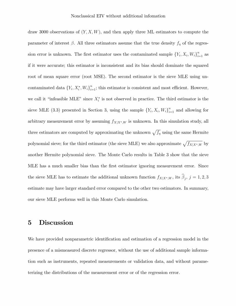
The Monte Carlo simulation consists of 400 repetitions. In each repetition, we randomly
Nonclassical EIV without additional infomation
draw 3000 observations of (Y;X;W ), and then apply three ML estimators to compute the
parameter of interest �. All three estimators assume that the true density f� of the regres-
sion error is unknown. The �rst estimator uses the contaminated sample fYi; Xi;Wigni=1 as
if it were accurate; this estimator is inconsistent and its bias should dominate the squared
root of mean square error (root MSE). The second estimator is the sieve MLE using un-
contaminated data fYi; X�i ;Wigni=1; this estimator is consistent and most e¢ cient. However,
we call it �infeasible MLE�since X�i is not observed in practice. The third estimator is the
sieve MLE (3.3) presented in Section 3, using the sample fYi; Xi;Wigni=1 and allowing for
arbitrary measurement error by assuming fXjX�;W is unknown. In this simulation study, all
three estimators are computed by approximating the unknownpf� using the same Hermite
polynomial sieve; for the third estimator (the sieve MLE) we also approximatepfXjX�;W by
another Hermite polynomial sieve. The Monte Carlo results in Table 3 show that the sieve
MLE has a much smaller bias than the �rst estimator ignoring measurement error. Since
the sieve MLE has to estimate the additional unknown function fXjX�;W , its b�j, j = 1; 2; 3estimate may have larger standard error compared to the other two estimators. In summary,
our sieve MLE performs well in this Monte Carlo simulation.
5 Discussion
We have provided nonparametric identi�cation and estimation of a regression model in the
presence of a mismeasured discrete regressor, without the use of additional sample informa-
tion such as instruments, repeated measurements or validation data, and without parame-
terizing the distributions of the measurement error or of the regression error.
Nonclassical EIV without additional infomation
Identi�cation mainly comes from the monotonicity of the regression function, the lim-
ited support of the mismeasured regressor, su¢ cient variation in the dependent variable,
and from some independence related assumptions regarding the regression model error. It
may be possible to extend these results to continuously distributed nonclassically mismea-
sured regressors, by replacing many of our matrix related assumptions and calculations with
corresponding linear operators.
APPENDIX. MATHEMATICAL PROOFS
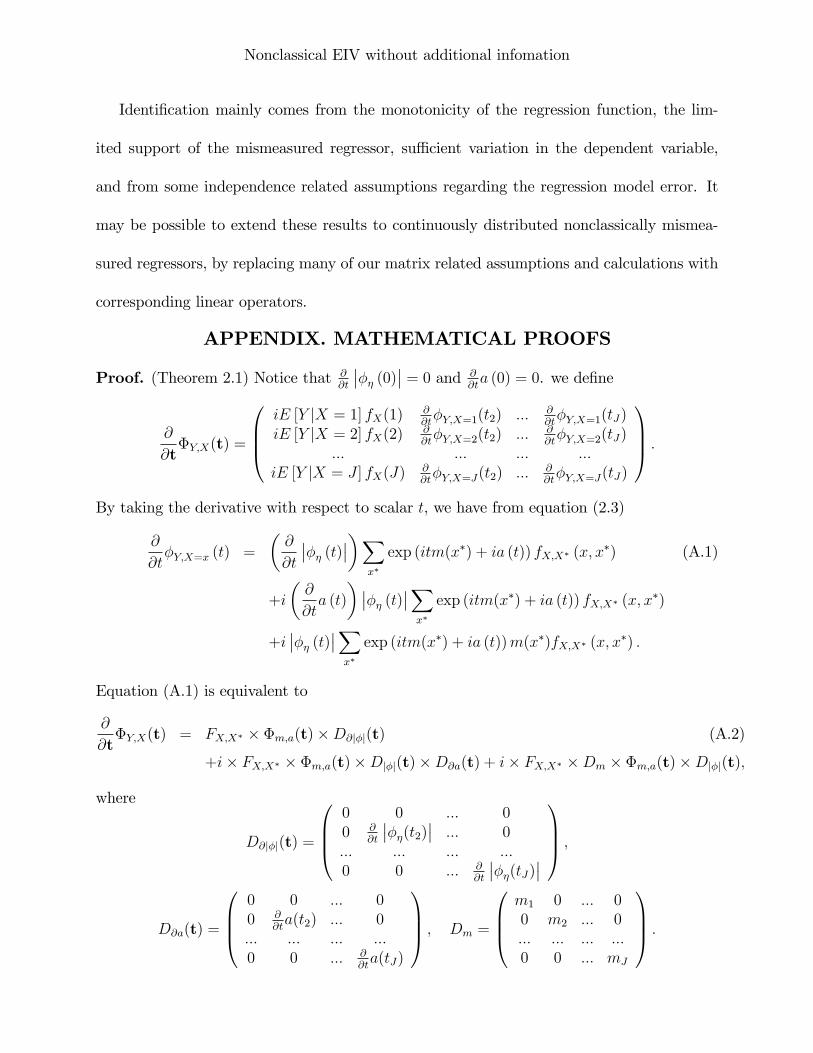
Proof. (Theorem 2.1) Notice that @@t
���� (0)�� = 0 and @@ta (0) = 0. we de�ne
@
@t�Y;X(t) =
0BB@iE [Y jX = 1] fX(1)
@@t�Y;X=1(t2) ::: @
@t�Y;X=1(tJ)
iE [Y jX = 2] fX(2)@@t�Y;X=2(t2) ::: @
@t�Y;X=2(tJ)
::: ::: ::: :::iE [Y jX = J ] fX(J)
@@t�Y;X=J(t2) ::: @
@t�Y;X=J(tJ)
1CCA :By taking the derivative with respect to scalar t, we have from equation (2.3)
@
@t�Y;X=x (t) =
�@
@t
���� (t)���Xx�
exp (itm(x�) + ia (t)) fX;X� (x; x�) (A.1)
+i
�@
@ta (t)
� ���� (t)��Xx�
exp (itm(x�) + ia (t)) fX;X� (x; x�)
+i���� (t)��X
x�
exp (itm(x�) + ia (t))m(x�)fX;X� (x; x�) :
Equation (A.1) is equivalent to
@
@t�Y;X(t) = FX;X� � �m;a(t)�D@j�j(t) (A.2)
+i� FX;X� � �m;a(t)�Dj�j(t)�D@a(t) + i� FX;X� �Dm � �m;a(t)�Dj�j(t);
where
D@j�j(t) =
0BB@0 0 ::: 00 @
@t
����(t2)�� ::: 0::: ::: ::: :::0 0 ::: @
@t
����(tJ)��1CCA ;
D@a(t) =
0BB@0 0 ::: 00 @
@ta(t2) ::: 0
::: ::: ::: :::0 0 ::: @
@ta(tJ)
1CCA ; Dm =
0BB@m1 0 ::: 00 m2 ::: 0::: ::: ::: :::0 0 ::: mJ
1CCA :
Nonclassical EIV without additional infomation
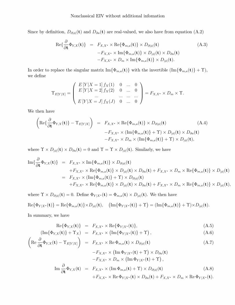
Since by de�nition, D@j�j(t) and D@a(t) are real-valued, we also have from equation (A.2)
Ref @@t�Y;X(t)g = FX;X� � Ref�m;a(t)g �D@j�j(t) (A.3)
�FX;X� � Imf�m;a(t)g �Dj�j(t)�D@a(t)
�FX;X� �Dm � Imf�m;a(t)g �Dj�j(t):
In order to replace the singular matrix Imf�m;a(t)g with the invertible (Imf�m;a(t)g+�),we de�ne
�E[Y jX] =
0BB@E [Y jX = 1] fX(1) 0 ::: 0E [Y jX = 2] fX(2) 0 ::: 0
::: ::: ::: :::E [Y jX = J ] fX(J) 0 ::: 0
1CCA = FX;X� �Dm ��:
We then have�Ref @
@t�Y;X(t)g ��E[Y jX]
�= FX;X� � Ref�m;a(t)g �D@j�j(t) (A.4)
�FX;X� � (Imf�m;a(t)g+�)�Dj�j(t)�D@a(t)
�FX;X� �Dm � (Imf�m;a(t)g+�)�Dj�j(t);
where ��Dj�j(t)�D@a(t) = 0 and � = ��Dj�j(t). Similarly, we have
Imf @@t�Y;X(t)g = FX;X� � Imf�m;a(t)g �D@j�j(t)
+FX;X� � Ref�m;a(t)g �Dj�j(t)�D@a(t) + FX;X� �Dm � Ref�m;a(t)g �Dj�j(t)
= FX;X� � (Imf�m;a(t)g+�)�D@j�j(t)
+FX;X� � Ref�m;a(t)g �Dj�j(t)�D@a(t) + FX;X� �Dm � Ref�m;a(t)g �Dj�j(t);
where ��D@j�j(t) = 0. De�ne �Y jX�(t) = �m;a(t)�Dj�j(t). We then have
Ref�Y jX�(t)g = Ref�m;a(t)g�Dj�j(t);�Imf�Y jX�(t)g+�
�= (Imf�m;a(t)g+�)�Dj�j(t):
In summary, we have
Ref�Y;X(t)g = FX;X� � Ref�Y jX�(t)g; (A.5)
(Imf�Y;X(t)g+�X) = FX;X� ��Imf�Y jX�(t)g+�
�; (A.6)�
Re@
@t�Y;X(t)��E[Y jX]
�= FX;X� � Re�m;a(t)�D@j�j(t) (A.7)
�FX;X� ��Im�Y jX�(t) + �
��D@a(t)
�FX;X� �Dm ��Im�Y jX�(t) + �
�;
Im@
@t�Y;X(t) = FX;X� � (Im�m;a(t) + �)�D@j�j(t) (A.8)
+FX;X� � Re�Y jX�(t)�D@a(t) + FX;X� �Dm � Re�Y jX�(t):
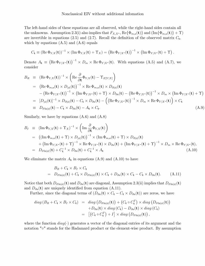
Nonclassical EIV without additional infomation
The left-hand sides of these equations are all observed, while the right-hand sides contain allthe unknowns. Assumption 2.3(i) also implies that FX;X�, Ref�m;a(t)g and (Imf�m;a(t)g+�)are invertible in equations (2.5) and (2.7). Recall the de�nition of the observed matrix Ct;which by equations (A.5) and (A.6) equals
Ct � (Re�Y;X(t))�1 � (Im�Y;X(t) + �X) =�Re�Y jX�(t)
��1 � �Im�Y jX�(t) + ��:
Denote At ��Re�Y jX�(t)
��1 � Dm � Re�Y jX�(t). With equations (A.5) and (A.7), weconsider
BR � (Re�Y;X(t))�1 �
�Re
@
@t�Y;X(t)��E[Y jX]
�=
�Re�m;a(t)�Dj�j(t)
��1 � Re�m;a(t)�D@j�j(t)
��Re�Y jX�(t)
��1 � �Im�Y jX�(t) + ���D@a(t)�
�Re�Y jX�(t)
��1 �Dm ��Im�Y jX�(t) + �
�= [Dj�j(t)]
�1 �D@j�j(t)� Ct �D@a(t)���Re�Y jX�(t)
��1 �Dm � Re�Y jX�(t)�� Ct
� D@ lnj�j(t)� Ct �D@a(t)� At � Ct: (A.9)
Similarly, we have by equations (A.6) and (A.8)
BI � (Im�Y;X(t) + �X)�1 �
�Im
@
@t�Y;X(t)
�=
�(Im�m;a(t) + �)�Dj�j(t)
��1 � (Im�m;a(t) + �)�D@j�j(t)
+�Im�Y jX�(t) + �
��1 � Re�Y jX�(t)�D@a(t) +�Im�Y jX�(t) + �
��1 �Dm � Re�Y jX�(t);
= D@ lnj�j(t) + C�1t �D@a(t) + C
�1t � At (A.10)
We eliminate the matrix At in equations (A.9) and (A.10) to have
BR + Ct �BI � Ct= D@ lnj�j(t) + Ct �D@ lnj�j(t)� Ct +D@a(t)� Ct � Ct �D@a(t): (A.11)
Notice that bothD@ lnj�j(t) andD@a(t) are diagonal, Assumption 2.3(ii) implies thatD@ lnj�j(t)
and D@a(t) are uniquely identi�ed from equation (A.11).Further, since the diagonal terms of (D@a(t)� Ct � Ct �D@a(t)) are zeros, we have
diag (BR + Ct �BI � Ct) = diag�D@ lnj�j(t)
�+�Ct � CTt
�� diag
�D@ lnj�j(t)
�+D@a(t)� diag (Ct)�D@a(t)� diag (Ct)
=��Ct � CTt
�+ I�� diag
�D@ lnj�j(t)
�;
where the function diag(�) generates a vector of the diagonal entries of its argument and thenotation "�" stands for the Hadamard product or the element-wise product. By assumption
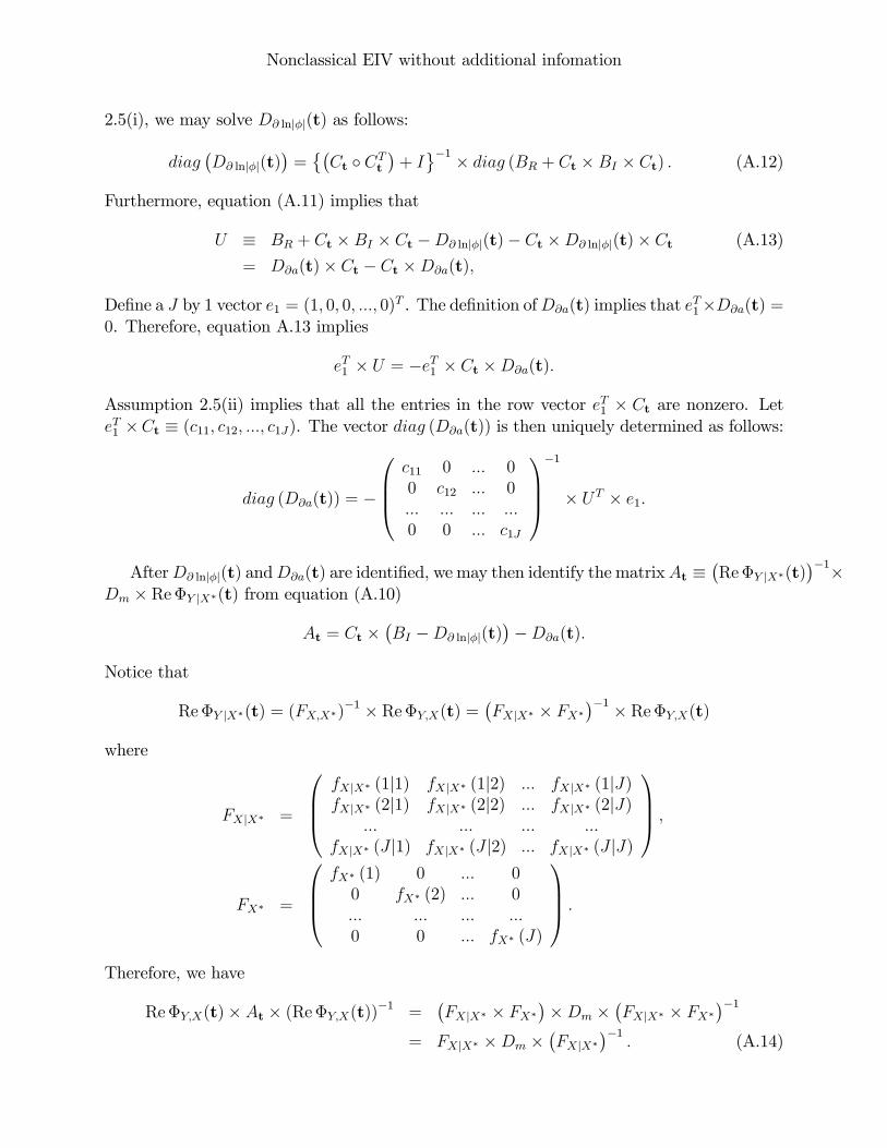
Nonclassical EIV without additional infomation
2.5(i), we may solve D@ lnj�j(t) as follows:
diag�D@ lnj�j(t)
�=��Ct � CTt
�+ I�1 � diag (BR + Ct �BI � Ct) : (A.12)
Furthermore, equation (A.11) implies that
U � BR + Ct �BI � Ct �D@ lnj�j(t)� Ct �D@ lnj�j(t)� Ct (A.13)
= D@a(t)� Ct � Ct �D@a(t);
De�ne a J by 1 vector e1 = (1; 0; 0; :::; 0)T . The de�nition ofD@a(t) implies that eT1�D@a(t) =0. Therefore, equation A.13 implies
eT1 � U = �eT1 � Ct �D@a(t):
Assumption 2.5(ii) implies that all the entries in the row vector eT1 � Ct are nonzero. LeteT1 �Ct � (c11; c12; :::; c1J). The vector diag (D@a(t)) is then uniquely determined as follows:
diag (D@a(t)) = �
0BB@c11 0 ::: 00 c12 ::: 0::: ::: ::: :::0 0 ::: c1J
1CCA�1
� UT � e1:
AfterD@ lnj�j(t) andD@a(t) are identi�ed, we may then identify the matrixAt ��Re�Y jX�(t)
��1�Dm � Re�Y jX�(t) from equation (A.10)
At = Ct ��BI �D@ lnj�j(t)
��D@a(t):
Notice that
Re�Y jX�(t) = (FX;X�)�1 � Re�Y;X(t) =�FXjX� � FX�
��1 � Re�Y;X(t)where
FXjX� =
0BB@fXjX� (1j1) fXjX� (1j2) ::: fXjX� (1jJ)fXjX� (2j1) fXjX� (2j2) ::: fXjX� (2jJ)
::: ::: ::: :::fXjX� (J j1) fXjX� (J j2) ::: fXjX� (J jJ)
1CCA ;
FX� =
0BB@fX� (1) 0 ::: 00 fX� (2) ::: 0::: ::: ::: :::0 0 ::: fX� (J)
1CCA :Therefore, we have
Re�Y;X(t)� At � (Re�Y;X(t))�1 =�FXjX� � FX�
��Dm �
�FXjX� � FX�
��1= FXjX� �Dm �
�FXjX�
��1: (A.14)
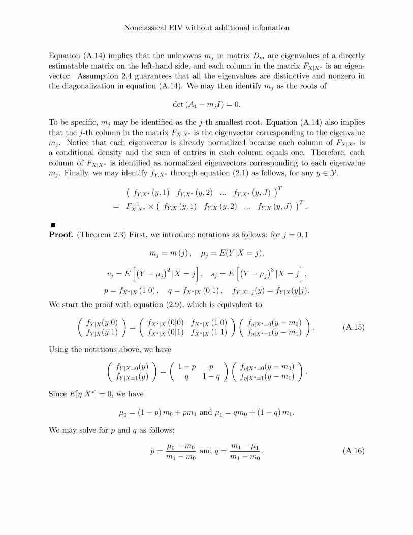
Nonclassical EIV without additional infomation
Equation (A.14) implies that the unknowns mj in matrix Dm are eigenvalues of a directlyestimatable matrix on the left-hand side, and each column in the matrix FXjX� is an eigen-vector. Assumption 2.4 guarantees that all the eigenvalues are distinctive and nonzero inthe diagonalization in equation (A.14). We may then identify mj as the roots of
det (At �mjI) = 0:
To be speci�c, mj may be identi�ed as the j-th smallest root. Equation (A.14) also impliesthat the j-th column in the matrix FXjX� is the eigenvector corresponding to the eigenvaluemj. Notice that each eigenvector is already normalized because each column of FXjX� isa conditional density and the sum of entries in each column equals one. Therefore, eachcolumn of FXjX� is identi�ed as normalized eigenvectors corresponding to each eigenvaluemj. Finally, we may identify fY;X� through equation (2.1) as follows, for any y 2 Y :�
fY;X� (y; 1) fY;X� (y; 2) ::: fY;X� (y; J)�T
= F�1XjX� ��fY;X (y; 1) fY;X (y; 2) ::: fY;X (y; J)
�T:
Proof. (Theorem 2.3) First, we introduce notations as follows: for j = 0; 1
mj = m (j) ; �j = E(Y jX = j);
vj = Eh�Y � �j
�2 jX = ji, sj = E
h�Y � �j
�3 jX = ji,
p = fX�jX (1j0) ; q = fX�jX (0j1) ; fY jX=j(y) = fY jX(yjj):
We start the proof with equation (2.9), which is equivalent to�fY jX(yj0)fY jX(yj1)
�=
�fX�jX (0j0) fX�jX (1j0)fX�jX (0j1) fX�jX (1j1)
��f�jX�=0(y �m0)f�jX�=1(y �m1)
�: (A.15)
Using the notations above, we have�fY jX=0(y)fY jX=1(y)
�=
�1� p pq 1� q
��f�jX�=0(y �m0)f�jX�=1(y �m1)
�:
Since E[�jX�] = 0, we have
�0 = (1� p)m0 + pm1 and �1 = qm0 + (1� q)m1:
We may solve for p and q as follows:
p =�0 �m0
m1 �m0
and q =m1 � �1m1 �m0
: (A.16)
Nonclassical EIV without additional infomation
We also have
1� p� q = 1��m1 �m0 + �0 � �1
m1 �m0
�=�1 � �0m1 �m0
:
Assumption 2.9 implies thatm1 � �1 > �0 � m0:
and �f�jX�=0(y �m0)f�jX�=1(y �m1)
�=
1
1� p� q
�1� q �p�q 1� p
��fY jX=0(y)fY jX=1(y)
�:
Plug-in the expression of p and q in equation (A.16), we have
�p1� p� q =
m0 � �0�1 � �0
;�q
1� p� q =�1 �m1
�1 � �0;
1� p1� p� q = 1�
�q1� p� q ;
1� q1� p� q = 1�
�p1� p� q ;
and �f�jX�=0(y �m0)f�jX�=1(y �m1)
�=
1� m0��0
�1��0m0��0�1��0
�1�m1
�1��01� �1�m1
�1��0
!�fY jX=0(y)fY jX=1(y)
�
=
�1�m0
�1��0m0��0�1��0
�1�m1
�1��0m1��0�1��0
!�fY jX=0(y)fY jX=1(y)
�:
In other words, we have for j = 0; 1
f�jX�=j(y) =�1 �mj
�1 � �0fY jX=0(y +mj) +
mj � �0�1 � �0
fY jX=1(y +mj): (A.17)
In summary, fX�jX (or p and q) and f�jX� are identi�ed if we can identifym0 andm1. Next, weshow thatm0 andm1 are indeed identi�ed. By assumption 2.10, we have E
��kjX�� = E ��k�
for k = 2; 3: For k = 2, we consider
v1 = E�(m(X�)� �1)
2 jX = 1�+ E
��2�
= E�m(X�)2jX = 1
�� �21 + E
��2�= qm2
0 + (1� q)m21 � �21 + E
��2�:
Similarly, we havev0 = (1� p)m2
0 + pm21 � �20 + E
��2�:
We eliminate E (�2) to obtain,
(1� p)m20 + pm
21 �
�v0 + �
20
�= qm2
0 + (1� q)m21 �
�v1 + �
21
�:
That is �v1 + �
21
���v0 + �
20
�= (1� p� q)
�m21 �m2
0
�;
Nonclassical EIV without additional infomation
We have shown that1� p� q = �1 � �0
m1 �m0
:
Thus, m1 and m0 satisfy the following linear equation:
m1 +m0 =(v1 + �
21)� (v0 + �20)�1 � �0
� C1:
This means we need one more restriction to identify m1 and m0.We consider
s1 = E�(Y � �1)
3 jX = 1�= E
�(m (X�)� �1)
3 jX = 1�+ E
��3�
= q (m0 � �1)3 + (1� q) (m1 � �1)
3 + E��3�
ands0 = (1� p) (m0 � �0)
3 + p (m1 � �0)3 + E
��3�:
We eliminate E (�2) in the two equations above to obtain,
(1� p) (m0 � �0)3 + p (m1 � �0)
3 � s0 = q (m0 � �1)3 + (1� q) (m1 � �1)
3 � s1
Plug in the expression of p and q in equation (A.16), we have
� (m1 � �0) (m0 � �0) (m1 +m0 � 2�0)�s0 = � (m1 � �1) (m0 � �1) (m1 +m0 � 2�1)�s1;
Since m1 +m0 = C1; we have
(C1 �m0 � �0) (m0 � �0) (C1 � 2�0) + s0 = (C1 �m0 � �1) (m0 � �1) (C1 � 2�1) + s1;
that is,
��m20 � �20
�(C1 � 2�0) + (m0 � �0)C1 (C1 � 2�0) + s0
= ��m20 � �21
�(C1 � 2�1) + (m0 � �1)C1 (C1 � 2�1) + s1
Moreover, we have
�2m20 (�1 � �0) + 2C1 (�1 � �0)m0
= �21 (C1 � 2�1)� �20 (C1 � 2�0)� �1C1 (C1 � 2�1) + �0C1 (C1 � 2�0) + s1 � s0=
��21 � �20
�C1 � 2
��31 � �30
�� (�1 � �0)C21 + 2
��21 � �20
�C1 + s1 � s0
Since (�1 � �0) > 0, we have
�2m20 + 2C1m0 = 3 (�1 + �0)C1 � 2
�31 � �30�1 � �0
� C21 +s1 � s0�1 � �0
:
Finally, we have
�2�m0 �
1
2C1
�2+ C2 = 0
Nonclassical EIV without additional infomation
where
C2 =3
2C21 � 3 (�1 + �0)C1 + 2
�31 � �30�1 � �0
� s1 � s0�1 � �0
=3
2[C1 � (�1 + �0)]
2 � 32(�1 + �0)
2 + 2��21 + �1�0 + �
20
�� s1 � s0�1 � �0
=3
2[C1 � (�1 + �0)]
2 +1
2(�1 � �0)
2 � s1 � s0�1 � �0
=1
2(�1 � �0)
2 +3
2
�v1 � v0�1 � �0
�2� s1 � s0�1 � �0
sj = Eh�Y � �j
�3 jX = ji
= E�Y 3jX = j
�� 3E
�Y 2jX = j
��j + 3�
3j � �3j
= E�Y 3jX = j
�� 3E
�Y 2jX = j
��j + 2�
3j
� �j � 3�j�j + 2�3j ,
C2 =3
2C21 � 3 (�1 + �0)C1 + 2
�31 � �30�1 � �0
� s1 � s0�1 � �0
=3
2C21 � 3 (�1 + �0)C1 + 2
�31 � �30�1 � �0
� �1 � 3�1�1 + 2�31 � (�0 � 3�0�0 + 2�30)�1 � �0
=3
2C21 � 3 (�1 + �0)C1 �
�1 � 3�1�1 � (�0 � 3�0�0)�1 � �0
=3
2C21 � 3 (�1 + �0)
�1 � �0�1 � �0
+3�1�1 � 3�0�0�1 � �0
� �1 � �0�1 � �0
=3
2
��1 � �0�1 � �0
�2� 3�0�1 � �1�0
�1 � �0� �1 � �0�1 � �0
Notice that we also have
�2�m1 �
1
2C1
�2+ C2 = 0;
which implies that m1 and m0 are two roots of this quadratic equation. Since m1 > m0, wehave
m0 =1
2C1 �
r1
2C2; m1 =
1
2C1 +
r1
2C2:
After we have identi�ed m0 and m1, p and q (or fX�jX) are identi�ed from equation (A.16),and the density f�(or fY jX�) is also identi�ed from equation (A.17). Thus, we have identi�edthe latent densities fY jX� and fX�jX from the observed density fY jX .
REFERENCES
Ai, C., and Chen, X. (2003), �E¢ cient Estimation of Models With Conditional Moment Restric-
Nonclassical EIV without additional infomation
tions Containing Unknown Functions,�Econometrica, 71, 1795-1843.
Bickel, P. J.; Ritov, Y., 1987, "E¢ cient estimation in the errors in variables model." Ann. Statist.15, no. 2, 513�540.
Bordes, L., S. Mottelet, and P. Vandekerkhove, 2006, "Semiparametric estimation of a two-component mixture model," Annals of Statistics, 34, 1204-232.
Bound, J. C. Brown and N. Mathiowetz, 2001, �Measurement error in survey data�, in Handbookof Econometrics, Vol. 5, ed. by J. Heckman and E. Leamer. North Holland.
Carroll, R.J., D. Puppert, C. Crainiceanu, T. Tostenson and M. Karagas, 2004), �Nonlinear andNonparametric Regression and Instrumental Variables,�Journal of the American StatisticalAssociation, 99 (467), pp. 736-750.
Carroll, R.J., D. Puppert, L. Stefanski and C. Crainiceanu, 2006, Measurement Error in NonlinearModels: A Modern Perspective, Second Edition, CRI.
Carroll, R.J. and L.A. Stefanski, 1990, �Approximate quasi-likelihood estimation in models withsurrogate predictors,�Journal of the American Statistical Association 85, pp. 652-663.
Chen, X. (2006): �Large Sample Sieve Estimation of Semi-nonparametric Models�, in J.J. Heck-man and E.E. Leamer (eds.), The Handbook of Econometrics, vol. 6. North-Holland, Ams-terdam, forthcoming.
Chen, X., H. Hong, and D. Nekipelov, 2007, �Measurement error models,�working paper of NewYork University and Stanford University, a survey prepared for the Journal of EconomicLiterature.
Chen, X., H. Hong, and E. Tamer, 2005, �Measurement error models with auxiliary data,�Reviewof Economic Studies, 72, pp. 343-366.
Chen, X., H. Hong, and A. Tarozzi (2007): �Semiparametric E¢ ciency in GMM Models withAuxiliary Data,�Annals of Statistics, forthcoming.
Cheng, C. L., Van Ness, J. W., 1999, Statistical Regression with Measurement Error, Arnold,London.
Fuller, W., 1987, Measurement error models. New York: John Wiley & Sons.
Geman, S., and Hwang, C. (1982), �Nonparametric Maximum Likelihood Estimation by theMethod of Sieves,�The Annals of Statistics, 10, 401-414.
Grenander, U. (1981), Abstract Inference, New York: Wiley Series.
Hansen, L.P. (1982): �Large Sample Properties of Generalized Method of Moments Estimators,�Econometrica, 50, 1029-1054.
Nonclassical EIV without additional infomation
Hausman, J., Ichimura, H., Newey, W., and Powell, J., 1991, �Identi�cation and estimation ofpolynomial errors-in-variables models,�Journal of Econometrics, 50, pp. 273-295.
Hsiao, C., 1991, �Identi�cation and estimation of dichotomous latent variables models using paneldata,�Review of Economic Studies 58, pp. 717-731.
Hu, Y. (2006): �Identi�cation and Estimation of Nonlinear Models with Misclassi�cation ErrorUsing Instrumental Variables,�Working Paper, University of Texas at Austin.
Hu, Y, and G. Ridder, 2006, �Estimation of Nonlinear Models with Measurement Error UsingMarginal Information,�Working Paper, University of Southern California.
Hu, Y, and S. Schennach, 2006,"Identi�cation and estimation of nonclassical nonlinear errors-in-variables models with continuous distributions using instruments," Cemmap Working PapersCWP17/06.
Kendall, M. and A. Stuart, 1979, The Advanced Theory of Statistics, Macmillan, New York, 4thedition.
Lee, L.-F., and J.H. Sepanski, 1995, �Estimation of linear and nonlinear errors-in-variables modelsusing validation data,�Journal of the American Statistical Association, 90 (429).
Lewbel, A., 1997, "Constructing Instruments for Regressions With Measurement Error When NoAdditional Data are Available, With an Application to Patents and R&D," Econometrica,65, 1201-1213.
Lewbel, A., 2007, �Estimation of average treatment e¤ects with misclassi�cation,�Econometrica,2007, 75, 537-551.
Li, T., 2002, �Robust and consistent estimation of nonlinear errors-in-variables models,�Journalof Econometrics, 110, pp. 1-26.
Li, T., and Q. Vuong, 1998, �Nonparametric estimation of the measurement error model usingmultiple indicators,�Journal of Multivariate Analysis, 65, pp. 139-165.
Liang, H., W. Hardle, and R. Carroll, 1999, �Estimation in a Semiparametric Partially LinearErrors-in-Variables Model,�The Annals of Statistics, Vol. 27, No. 5, 1519-1535.
Liang, H.; Wang, N., 2005, "Partially linear single-index measurement error models," Statist.Sinica 15, no. 1, 99�116.
Mahajan, A. (2006): �Identi�cation and estimation of regression models with misclassi�cation,�Econometrica, vol. 74, pp. 631-665.
Murphy, S. A. and Van der Vaart, A. W. 1996, "Likelihood inference in the errors-in-variablesmodel." J. Multivariate Anal. 59, no. 1, 81-08.
Murphy, S. A. and Van der Vaart, A. W. 2000, "On Pro�le Likelihood�, Journal of the AmericanStatistical Association, 95, 449-486.
Nonclassical EIV without additional infomation
Newey, W.K. and J. Powell (2003): �Instrumental Variables Estimation for Nonparametric Mod-els,�Econometrica, 71, 1565-1578.
Reiersol, O. (1950): �Identi�ability of a Linear Relation between Variables Which Are Subject toError,�Econometrica, 18, 375-389.
Schennach, S. (2004): �Estimation of Nonlinear Models with Measurement Error,�Econometrica,72, 33-75.
Shen, X. (1997), �On Methods of Sieves and Penalization,�The Annals of Statistics, 25, 2555-2591.
Shen, X., and Wong, W. (1994), �Convergence Rate of Sieve Estimates,�The Annals of Statistics,22, 580-615.
Taupin, M. L., 2001, �Semi-parametric estimation in the nonlinear structural errors-in-variablesmodel,�Annals of Statistics, 29, pp. 66-93.
Van de Geer, S. (1993), �Hellinger-Consistency of Certain Nonparametric Maximum LikelihoodEstimators,�The Annals of Statistics, 21, 14-44.
Van de Geer, S. (2000), Empirical Processes in M-estimation, Cambridge University Press.
Van der Vaart, A. and J. Wellner (1996): Weak Convergence and Empirical Processes: withApplications to Statistics. New York: Springer-Verlag.
Wang, L., 2004, "Estimation of nonlinear models with Berkson measurement errors," The Annalsof Statistics 32, no. 6, 2559�2579.
Wang, N., X. Lin, R. Gutierrez, and R. Carroll, 1998, "Bias analysis and SIMEX approach ingeneralized linear mixed measurement error models," J. Amer. Statist. Assoc. 93, no. 441,249�261.
Wansbeek, T. and E. Meijer, 2000, Measurement Error and Latent Variables in Econometrics.New York: North Holland.
Wong, W., and Shen, X. (1995), �Probability Inequalities for Likelihood Ratios and ConvergenceRates for Sieve MLE�s,�The Annals of Statistics, 23, 339-362.
Nonclassical EIV without additional infomation
Table 1: Simulation resultsExample 1Value of x�: 1 2 3 4
Regression function m(x�):�true value 1.3500 2.8000 5.9500 11.400�mean estimate 1.2984 2.9146 6.0138 11.433�standard error 0.2947 0.3488 0.2999 0.2957
Marginal distribution Pr (x�):�true value 0.2 0.3 0.3 0.2�mean estimate 0.2159 0.2818 0.3040 0.1983�standard error 0.1007 0.2367 0.1741 0.0153
Misclasi�cation Prob. fxjx� (�jx�):�true value 0.6 0.2 0.1 0.1
0.2 0.6 0.1 0.10.1 0.1 0.7 0.10.1 0.1 0.1 0.7
�mean estimate 0.5825 0.2008 0.0991 0.09860.2181 0.5888 0.1012 0.09740.0994 0.1137 0.6958 0.09930.1001 0.0967 0.1039 0.7047
�standard error 0.0788 0.0546 0.0201 0.01400.0780 0.0788 0.0336 0.02060.0387 0.0574 0.0515 0.02810.0201 0.0192 0.0293 0.0321
Nonclassical EIV without additional infomation
Table 2: Simulation resultsExample 2Value of x�: 1 2 3 4
Regression function m(x�):�true value 1.3500 2.8000 5.9500 11.400�mean estimate 1.2320 3.1627 6.1642 11.514�standard error 0.4648 0.7580 0.7194 0.6940
Marginal distribution Pr (x�):�true value 0.2 0.3 0.3 0.2�mean estimate 0.2244 0.3094 0.2657 0.2005�standard error 0.1498 0.1992 0.1778 0.0957
Misclasi�cation Prob. fxjx� (�jx�):�true value 0.5220 0.1262 0.2180 0.2994
0.1881 0.4968 0.1719 0.24890.1829 0.1699 0.4126 0.03810.1070 0.2071 0.1976 0.4137
�mean estimate 0.4761 0.1545 0.2214 0.29690.2298 0.4502 0.1668 0.24550.1744 0.1980 0.4063 0.04370.1197 0.1973 0.2056 0.4140
�standard error 0.1053 0.0696 0.0343 0.02150.0806 0.0771 0.0459 0.02620.0369 0.0528 0.0573 0.03130.0327 0.0221 0.0327 0.0238
Nonclassical EIV without additional infomation
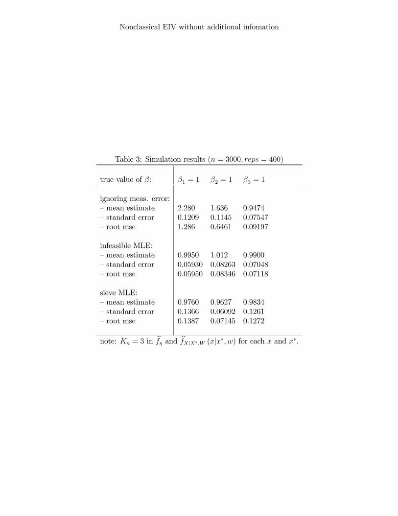
Table 3: Simulation results (n = 3000; reps = 400)
true value of �: �1 = 1 �2 = 1 �3 = 1
ignoring meas. error:�mean estimate 2.280 1.636 0.9474�standard error 0.1209 0.1145 0.07547�root mse 1.286 0.6461 0.09197
infeasible MLE:�mean estimate 0.9950 1.012 0.9900�standard error 0.05930 0.08263 0.07048�root mse 0.05950 0.08346 0.07118
sieve MLE:�mean estimate 0.9760 0.9627 0.9834�standard error 0.1366 0.06092 0.1261�root mse 0.1387 0.07145 0.1272
note: Kn = 3 in bf� and bfXjX�;W (xjx�; w) for each x and x�: