
The Three SaaS Levers that Drive Growth and Keep You From Plateauing
Monetary Policy, Liquidity, and Growth�
Philippe Aghiony, Emmanuel Farhiz, Enisse Kharroubix
19th September 2011
Abstract
In this paper, we use cross-industry, cross-country panel data to test whether industry growth is
positively a¤ected by the interaction between the reactivity of real short term interest rates to the business
cycle and industry-level measures of �nancial constraints. Financial constraints are measured, either by
the extent to which the domestic industry is prone to being "credit constrained", or by the extent to
which it is prone to being "liquidity constrained". Our main �ndings are that: (i) the interaction between
credit or liquidity constraints in an industry and monetary policy countercyclicality in the domestic
country, has a positive, signi�cant, and robust impact on the average annual rate of labor productivity
in the domestic industry; (ii) these interaction e¤ects tend to be more signi�cant in downturns than in
upturns; (iii) �nally, while in downturns both, high-tech and low-tech sectors seem to bene�t from more
countercyclical monetary policies, in upturns it is the high-tech sectors which bene�t most.
1 Introduction
Macroeconomic textbooks usually draw a clear distinction between long run growth and its main determ-
inants on the one hand, and macroeconomic policies (�scal and monetary) aimed at achieving short run
stabilization on the other. In this paper we argue instead that more countercyclical monetary policies,
whereby real short term interest rates are lower in recessions and higher in booms, have a more positive long
run growth e¤ect in industries that are more prone to being credit-constrained or in industries that are more
prone to being liquidity-constrained.
In the �rst part of the paper, we present a simple model of an economy populated by entrepreneurs
who must borrow from outside investors to �nance their investments. At the initial investment stage,
entrepreneurs may borrow on the credit market if they need to invest more than their initial wealth. Credit
markets are imperfect due to the limited pledgeability of the returns from the project to outside investors (as
�The views expressed here are those of the authors and do not necessarily represent the views of the Bank for International
Settlements, the Banque de France nor any institution belonging to the Eurosystem.yHarvard University and NBERzHarvard University and NBERxBank of International Settlements
1
in Holmstrom and Tirole, 1997). Once they are initiated, projects may either turn be "fast" and yield full
returns within one period after the initial investment has been sunk, or they may turn out to be "slow" and
require some reinvestment in order to yields returns within two periods. The probability 1� � of a project
being slow, and therefore requiring reinvestment, measures the degree of potential liquidity dependence of
the economy in the model. However, the actual degree of liquidity dependence will also depend upon the
aggregate state of the economy. More precisely, we assume that if the economy as a whole is in a boom, then
short-run pro�ts are su¢ cient for entrepreneurs to �nance the required reinvestment whenever they need to
do so (i.e whenever their project turns out to slow); in contrast, if the economy is in a slump, then reinvesting
requires that the entrepreneur downsize and delever her project (and therefore reduce her expected end-of-
project returns) in order to generate cash to pay for the reinvestment. However, the entrepreneur can
somewhat reduce the need for deleveraging in case the project is slow, if she decides ex ante to invest part of
her initial funds in liquid assets. Hoarding more liquidity reduces the need for ex post downsizing but this
comes at the expense of reducing the initial size of the project.
A more countercyclical interest rate policy enhances ex ante investment by reducing the amount of
liquidity entrepreneurs need to hoard to weather liquidity shocks when the economy is in a slump. The model
generate two main predictions. First, the lower the fraction of returns that can be pledged to outside investors,
the more investment enhancing it is for the government to implement a more countercyclical interest policy.
Second, the higher the liquidity risk measured by the probability (1� �); the more investment enhancing it
is for the government to conduct a more countercyclical interest rate policy. Third, the di¤erential e¤ect of
more countercyclical interest rates across �rms with di¤erent degrees of liquidity dependence, is stronger in
recessions than in expansions.
In the second part of the paper, we take these predictions to the data. Speci�cally, we build on the
methodology developed in the seminal paper by Rajan and Zingales (1998) and use cross-industry, cross-
country panel data to test whether industry growth is positively a¤ected by the interaction between domestic
monetary policy cyclicality (i.e the domestic reactivity of short-run real interest rates to the business cycle,
which is computed at country level) and industry-level measures of �nancial constraints that computed for
each corresponding industry in the United States. This approach provides a clear and net way to deal
with causality issues. Indeed, any negative correlation one might observe between the countercyclicality of
macroeconomic policy and average long run growth of an industry (or a country), might equally re�ect the
e¤ect of countercyclical interest rate policy on growth or the e¤ect of growth on a country�s ability to pursue
more countercyclical interest rate policies. However, what makes us reasonably con�dent that our regression
results capture a causal link from domestic countercyclical monetary policy to industry growth, is the fact
that: (i) we look at the e¤ect of macroeconomic policies implemented at the country level on industry-level
growth; (ii) individual industries are small compared to the overall economy so that we can con�dently rule
out the possibility that growth at the industry level should a¤ect the cyclical pattern of macroeconomic
policy at country level; (iii) our �nancial constraint variables are computed for US industries and therefore
2
are unlikely to be a¤ected by policies and outcomes in other countries.
Financial constraints at industry level are measured, either by the extent to which the corresponding
industry in the US is dependent on external �nance or displays low levels of asset tangibility (these two
measures capture the extent to which the domestic industry is prone to being credit constrained), or by the
extent to which the corresponding industry in the US shows high labor costs to sales or high inventories to
sales ration (i.e the extent to which the industry is prone to being liquidity constrained). Our main empirical
�nding is that the interaction between credit or liquidity constraints in an industry and monetary policy
countercyclicality in the domestic country, has a positive, signi�cant, and robust impact on the average annual
rate of labor productivity in the domestic industry. More speci�cally, the higher the extent to which the
corresponding industry in the United States relies on external �nance, or the lower the asset tangibility of the
corresponding sector in the United States, or the more liquidity dependent the corresponding US industry
is, the more growth-enhancing in the domestic industry it is to pursue a more countercyclical monetary
policy. Moreover, we show that the interaction e¤ects between monetary policy countercyclicality and each
of these various measures of credit and liquidity constraints, tend to be more signi�cant in downturns than in
upturns, and that these e¤ects are robust to controlling for the interaction between these measures of �nancial
constraints and country-level economic variables such as in�ation, �nancial development, and the size of
government which are likely to a¤ect the country�s ability to pursue more countercyclical macroeconomic
policies. Finally, we �nd that while in downturns both, high-tech and low-tech sectors seem to bene�t from
more countercyclical monetary policies, i.e from lower real short-run interest rates in downturns, in upturns
it is the high-tech sectors which bene�t most from more countercyclical monetary policy, i.e from higher
short-run interest rates. In other words, there is a cost of having low short-run interest rates in booms,
namely that of allocating to much capital to low-tech sectors at the expense of high-tech sectors.
The paper relates to several strands of literature. First, to the literature on macroeconomic volatility and
growth. A benchmark paper in this literature is Ramey and Ramey (1995) who �nd a negative correlation
in cross-country regressions between volatility and long-run growth. A �rst model to generate the prediction
that the correlation between long-run growth and volatility should be negative, is Acemoglu and Zilibotti
(1997) who point to low �nancial development as a factor that could both, reduce long-run growth and
increase the volatility of the economy. Acemoglu et al (2003) and Easterly (2005) hold that both, high
volatility and low long-run growth do not directly arise from policy decisions but rather from bad institutions.
Our paper contributes to this debate by showing a signi�cant growth e¤ect of more countercyclical monetary
policies on industries which are all located in OECD countries with similar property right and political
institutions.1
Second, we contribute to the literature on monetary policy design. In our model, monetary policy
1See also Aghion et al (2006) who analyze the relationship between long-run growth and the choice of exchange-rate regime;
and Aghion, Hemous and Kharroubi (2009) who show that more countercyclical �scal policies a¤ect growth more signi�cantly
in sectors whose US counterparts are more credit constrained.
3
operates through a version of the credit channel (see Bernanke and Gertler 1995 for a review of the credit
channel literature).2 But more speci�cally, our model builds on the macroeconomic literature on liquidity (e.g
Woodford 1990 and Holmstrom and Tirole 1998). This literature has emphasized the role of governments in
providing possibly contingent stores of value that cannot be created by the private sector. Like in Holmstrom
and Tirole, liquidity provision in our paper is modeled as a redistribution from consumers to �rms in the bad
state of nature; however, here it is an ex post redistribution rather than an ex ante one in Holmstrom and
Tirole. This perspective is shared with Farhi and Tirole (2011), however their focus is on time inconsistency
and ex ante regulation; also in their model, unlike in ours, there is no liquidity premium and therefore, under
full government commitment, there is no role for a countercyclical interest rate policy.
The paper is organized as follows. Section 2 outlays the model. Section 3 presents the empirical analysis.
It �rst details the methodology and the data used. Then it presents the main empirical results. Section 4
concludes. Finally, proofs and sample and estimation details are contained in the Appendix.
2 Model
2.1 Model setup
There are three periods, t = 0; 1; 2. Entrepreneurs have utility function U = E[c2] , where c2 is their date-2
consumption. They are protected by limited liability and their only endowment is their wealth A at date 0.
Their technology set exhibits constant returns to scale. At date 0 they choose their investment scale i > 0.
At date 1, uncertainty is realized: the aggregate state is either good (G) or bad (B), and the �rm is
either intact or experiences a liquidity shock. The date-0 probability of the good state is �, and the date-0
probability of a �rm experiencing a liquidity shock is 1� �. Both events are independent.
At date 1, a cash �ow �i accrues to the entrepreneur where, depending on the aggregate state, � 2
f�G; �Bg. This cash �ow is not pledgeable to outside investors. If the project is intact, the investment
delivers at date 1; it then yields, besides the cash �ow �i, a payo¤ of �1i, of which �0i is pledgeable to
investors.3 If the project is distressed, besides the except for the cash �ow �i, it yields a payo¤ at date 2 if
fresh resources j � i are reinvested. It then delivers at date 2 a payo¤ of �1j, of which �0j is pledgeable to
investors.
The following assumption is necessary to ensure that entrepreneurs are liquidity constrained and must
invest at a �nite scale.
Assumption 1 (liquidity constraint) �0 < minfR0; RG1 ; RB1 g:2There are two versions of the credit channel : the "balance sheet channel" and the "bank lending channel". Our model
features the balance sheet channel, focusing more on the e¤ect of interest rates on �rms�borrowing capacity.3As usual, the �agency wedge� �1 � �0 can be motivated in multiple ways, including limited commitment, private bene�ts
or incentives to counter moral hazard (see for example Holmström and Tirole 2010).
4
The interest rate is a key determinant of the collateral value of a project. It plays an important role in
determining the initial investment scale i as well as the reinvestment scale j. The gross rate of interest is
equal to R0 between dates 0 and 1, and R1 between dates 1 and 2; where R1 2 fRG1 ; RB1 g depending on the
aggregate state.
The following assumption will guarantee that: (i) in the good state, date-1 cash �ows will be enough
to cover liquidity needs and reinvest at full scale in the event of a liquidity shock, even with no hoarded
liquidity or issuance of new securities; and (ii) in the bad state, date-1 cash �ows will not be enough to cover
liquidity needs and reinvest at full scale so that downsizing will take place if no liquidity is hoarded at date
0.
Assumption 2 (cash-�ows) �G > 1 and 1� �0=RB1 > �B :
Because cash �ows are not enough to cover liquidity shocks in the bad state, entrepreneurs might wish
to engage in liquidity policy. They can purchase an asset that pays o¤ xi at date 1 in case of a liquidity
shock in the bad state. The date-0 cost of this liquidity is q(1 � �)(1 � �)i=R0, where q � 1: When q > 1,
the date-0 cost of this liquidity is greater than (1� �)(1� �)i=R0. The corresponding liquidity premium is
denoted by q � 1. This captures a situation where aggregate liquidity is scarce as in Holmström and Tirole
(1997). Alternatively, one can imagine that liquidity needs to be hoarded in the form of an instrument with
a high degree of market liquidity: the entrepreneur needs to be able to sell it quickly, without its losing much
value. Such instruments typically command a liquidity premium, for which q � 1 could be a stand in.
Assumption 3 in the Appendix guarantees that the projects are attractive enough that entrepreneurs will
always invest all their net worth.
At the core of the model is a maturity mismatch issue, where a long-term project requires occasional
reinvestments. The entrepreneur has to compromise between initial investment scale i and reinvestment
scale j in the event of a liquidity shock. Maximizing initial scale i requires minimizing hoarded liquidity
and exhausting reserves of pledgeable income. This in turn forces the entrepreneur to downsize and delever
in the event of a liquidity shock. Conversely, maximizing liquidity to mitigate maturity mismatch requires
sacri�cing initial scale i.
Besides short term pro�ts �i, liquidity xi represents cash available at date 1 in the event of a liquidity
shock (x is the analog of a liquidity ratio). We assume that any potential surplus of cash over liquidity
needs for reinvestment is consumed by entrepreneurs. The policy of pledging all cash that is unneeded for
reinvestment is always weakly optimal. Pledging less is also optimal (and leads to the same allocation)
if the entrepreneur has no alternative use of the unneeded cash to distributing to investors. However, if
the entrepreneur can divert (even an arbitrarily small) fraction of the extra cash for her own bene�t, then
pledging the entire unneeded cash is strictly optimal.
At date 1, in the bad state, if a liquidity shock hits, the entrepreneur can dilute initial investors by issuing
5
new securities against the date-2 pledgeable income �0j, and so its continuation j 2 [0; i] must satisfy:
j � (x+ �B)i+ �0j
RB1
yielding continuation scale:
j = min
(x+ �B
1� �0RB1
, 1
)i:
This formula captures the fact that lower interest rates facilitate re�nancing. An entrepreneur would never
choose to have excess liquidity and so we restrict our attention to x 2 [0; 1� �0=RB1 � �B ].
The entrepreneur needs to raise i � A from outside investors at date 0. If no liquidity shock hits,
the entrepreneur returns �0i to these investors at date 1. If a liquidity shock hits in the good state, the
entrepreneur returns �0i to these investors at date 2. If a liquidity shock hits in the bad state, these
investors are committed to inject additional funds xi; moreover, they are fully diluted. As a result, its
borrowing capacity at date 0 is given by:
i�A = ��0iR0
+ �(1� �) �0R0RG1
i� (1� �)(1� �)qxiR0
i.e.
i =A
1� � �0R0� �(1� �) �0
R0RG1+ (1� �) (1� �) qxR0
:
Assumption 4 in the Appendix guarantees that the entrepreneur optimally chooses to hoard enough
liquidity x = 1� �0=RB1 � �B to withstand a liquidity shock in the bad state without downsizing.
Our proxy for long-run investment in this model is the �rm equilibrium investment, which is equal to
i = sA; where:
s =1
1� � �0R0� �(1� �) �0
R0RG1+ (1� �) (1� �) q
�1��BR0
� �0R0RB
1
� :This variable captures long run growth in this model.
2.2 Illiquidity and countercyclical interest rate policy
We want to derive comparative static results with respect to the cyclicality of interest rate policy. For this
purpose, it will prove useful to adopt the following parametrization: RB = R , RG = R= , and R0 = R.
We take � 1 to be our measure of the cyclicality of interest rate policy: a low indicates a countercyclical
interest rate policy. We can then compute size
s =1
1� ��0R � �(1� �)�0 R2 + (1� �) (1� �) q
�1��BR � �0
R2
� : (1)
Proposition 1 Suppose that � < �̂ �q=(q + 2). Then @2 log s@�0@
> 0:
Proof. It is easy to see that
@ log s
@ = �
(1� �)h�� �0R2 + (1� �)q �0
R2 2
i1� �0
R + (1� �)h�0R � �
�0 R2 + (1� �)q
�1��BR � �0
R2
�i :6
Dividing the numerator and denominator of this expression by �0; we have
@ log s
@ = �
(1� �)h�� 1
R2 + (1� �)q 1R2 2
i1�0� 1
R + (1� �)h1R � �
R2 + (1� �)q
�1��BR�0
� 1R2
�i ;from which we immediately see that whenever the numerator is positive, then
@2 log s
@�0@ > 0:
This establishes the proposition.
Thus countercyclical interest rate policy encourages investment by �rms that face tighter credit con-
straints as inversely measured by the fraction of pledgeable income �0: Next, we look at the interaction
between countercyclical interest rate policy and �rms�vulnerability to liquidity shocks. Countercyclical in-
terest policy helps the re�nancing of �rms that experience a liquidity shock in the bad state. It also hurts the
re�nancing of �rms that experience a liquidity shock in the good state. However, it helps the former more
than it hurts the later, since �rms do not need to hoard costly liquidity for the good state but do for the bad
state. Indeed, in the good state, they can �nance their liquidity needs with their short term cash �ows. It
is then natural to expect more liquidity dependent �rms (�rms with a higher probability 1�� of a liquidity
shock) to bene�t disproportionately from a more countercyclical interest rate policy if the probability of the
bad state 1�� is high enough, and if the liquidity premium q� 1 is high enough. The following proposition
formalizes this insight.
Proposition 2 Suppose that � < �̂ �q=(q + 2). Then @2 log s@(1��)@ < 0:
Proof. We start again from:
@ log s
@ = �
(1� �)h�� �0R2 + (1� �)q �0
R2 2
i1� �0
R + (1� �)h�0R � �
�0 R2 + (1� �)q
�1��BR � �0
R2
�i :This implies that
@2 log s
@(1� �)@ = �
�1� �0
R
� �0R2
h��+ (1� �)q 1 2
in1� �0
R + (1� �)h�0R � �
�0 R2 + (1� �)q
�1��BR � �0
R2
�io2 :The result immediately follows.
A more countercyclical interest rate policy reduces the amount of liquidity 1��BR � �0
R2 that entrepreneurs
need to hoard to weather liquidity shocks in the bad state. This releases more pledgeable income for more
liquidity dependent �rms (�rms with a higher 1 � �) as long as the probability of the bad state 1 � � and
the liquidity premium q � 1 are both su¢ ciently high. As a result, those �rms can expand in size more.
We now want to investigate how this comparative static result is a¤ected by the state of the business
cycle. We view expansions and recessions as corresponding to di¤erent values of �: in an expansion, the
probability � of the good state is high and it is low in a recession. The next proposition establishes that
7
the di¤erential e¤ect of countercyclical interest rate policy across �rms with di¤erent degrees of liquidity
dependence is stronger in recessions than in expansions.
Proposition 3 There exists ~� < �̂ such that for all � 2 (~�; �̂); @3 log s@�@(1��)@ > 0.
Proof. We have
@2 log s
@(1� �)@ = �
�1� �0
R
� �0R2
hq 2 � �
�1 + q
2
�in1� ��0R + (1� �)q
�1��BR � �0
R2
�� � (1� �)
h�0 R2 + q
�1��BR � �0
R2
�io2 :This expression is �rst decreasing in � and then increasing in �. The minimum occurs at � = ~� where
~� =��1 + q
2
� h1� ��0R + (1� �)q
�1��BR � �0
R2
�i+ 2 q
2 (1� �)h�0 R2 + q
�1��BR � �0
R2
�i�1 + q
2
�(1� �)
h�0 R2 + q
�1��BR � �0
R2
�i :
It is easily veri�ed that ~� < �̂.
Propositions 1, 2 and 3 summarize the key comparative statics of the model that we wish to con�rm in
the data.
3 Empirical analysis
3.1 Methodology and data
Our dependent variable is the average annual growth rate in labor productivity in industry j in country k for
the period 1995-2005.4 We introduce industry and country �xed e¤ects f�j ; �kg to control for unobserved
heterogeneity across industries and across countries. The variable of interest, (ic)j�(mpc)k, is the interaction
between industry j�s intrinsic characteristic and the degree of (counter) cyclicality of monetary policy in
country k over the same time period of time as that over which industry growth rates are computed, here
1995-2005. Finally, we control for initial conditions by including the ratio of labor productivity in industry
j in country k to labor productivity in the overall manufacturing sector in country k at the beginning of the
period, i.e. in 1995. Denoting ytjk (resp. ytk) labor productivity in industry j (resp. in total manufacturing)
in country k at time t, and letting "jk denote the error term, our baseline estimation equation is expressed
as follows:ln(y05jk)� ln(y95jk)
10= �j + �k + (ic)j � (mpc)k � � ln
y95jky95k
!+ "jk: (2)
Now, turning to the stabilization policy cyclicality measure, (mpc)k , in country k, it is estimated
as the change in monetary policy due a change in the domestic output gap. We therefore use country-level
data to estimate the following country-by-country �auxiliary�equation over the time period 1995-2005:
rsirkt = �k + (mpc)k:zkt + ukt; (3)4We will be using two measures of labor productivity, either per worker or per hour workers. Both measures will provide
very consistent results. Some results where the dependent variable is real value added will also be presented.
8
where rsirkt is the real short term interest rate in country k at time t �de�ned as the di¤erence between
the three months policy interest rate set by the central bank and the 3-months annualized in�ation rate-
; zkt measures the output gap in country k at time t (that is, the percentage di¤erence between actual
and potential GDP). It therefore represents the country�s current position in the cycle;5 �k is a constant;
and ukt is an error term. For example, a positive (resp. negative) regression coe¢ cient (mpc)k re�ects
a countercyclical (pro-cyclical) monetary policy as the short term cost of capital tends to increase (resp.
decrease) when the economy�s outlook improves (resp. deteriorates).
It has become standard in the literature to estimate Taylor rules where the nominal short term interest
rate (nsir) is a function of in�ation � and the output gap z.
nsirkt = �k + ��kt + (mpctr)k:zkt + ukt (4)
We have made the choice of using Taylor rules as auxiliary -robustness- equations, our reason being that for
most countries, interest rates and in�ation rates are not stationary variables, while the di¤erence between the
interest rate and the in�ation rate is stationary. Hence, the cyclicality estimates obtained from our procedure
are less likely to be biased than those we would obtain from using Taylor rules as auxiliary equations. This
also explains why we focused on a relatively recent period, namely 1995-2005. Had we extended the sample
period to the early nineties, even the real short term interest rate would become non-stationary.
Yet, as alternative robustness checks, we introduce two di¤erent alternative auxiliary regressions designed
to take into account either past or future persistence. In the �rst variant (4), we control for the one-quarter-
lagged real short term interest rate:
rsirkt = �k + �rsirkt�1 + (mpc)k:zkt + ukt: (5)
In the second variant, we control for the one-quarter-forward real short term interest rate:
rsirkt = �k + �rsirkt+1 + (mpc)k:zkt + ukt: (6)
Last, when two countries di¤er in their monetary policy cyclicality estimates, it is worth knowing whether
this di¤erence comes mainly from what happens in upturns versus downturns. To this end, we shall estimate
the following third variant of the auxiliary equation:
rsirkt = �k + (mpc+)k:z
+kt + (mpc
�)k:z�kt + ukt: (7)
Here, z+ktq is equal to the output gap if the output gap is higher than its historical median and it is equal to
zero otherwise. Similarly, z�ktq is equal to the output gap if the output gap is lower than its historical median
5The output gap is estimated as the di¤erence between the log of real GDP and the HP �ltered series of the log of real
GDP, using the standard smoothing parameter for quarterly data. Moreover the time sample ends up in 2005 in order to avoid
end-of-sample problems in the estimated of trend GDP and output gap. In other words, we have enough data both at the
before the beginning and after the end of our sample to estimate properly the cycle by the beginning and the end of our sample
period.
9
and it is equal to zero otherwise. The estimated coe¢ cient mpc+ (resp. mpc�) measures how strongly the
real interest rate reacts to variations in the output gap during an upturn (respectively during a downturn).
This regression will then helps us determine whether the growth e¤ect of monetary policy cyclicality, if any,
comes from what happens during upturns versus downturns.
Turning now to industry-speci�c characteristics, we follow Rajan and Zingales (1998) in using �rm-
level data pertaining to the United States. We concentrate two set of �nancial constraints a¤ecting �rms,
borrowing constraints and liquidity constraints. We consider two di¤erent proxies for borrowing constraints,
namely external �nancial dependence and asset tangibility. External �nancial dependence is measured as
the median ratio across �rms belonging to the corresponding industry in the US of capital expenditures
minus current cash �ow to total capital expenditures. Asset tangibility is measured as the median ratio
across �rms in the corresponding industry in the US of the value of net property, plant, and equipment to
total assets. To measure liquidity constraints, we consider two alternative indicators. First, the median ratio
across �rms belonging to the corresponding industry in the US of inventories to total sales.6 Second, the
median ratio across �rms in the corresponding industry in the US of labor costs to total sales. The �rst two
measures give an indication about an industry need or di¢ culty to raise external �nance and as such can be
considered as proxies for the industry�s borrowing constraints. The last three measures give an indication
about an industry�s need for short term �nancing. For example, industries with a larger ratio of labor costs
to sales have larger payments to make on a monthly basis and should therefore face larger needs for short
term re�nancing. Similarly, industries have higher needs for liquidity when they need to maintain larger
inventories as inventories are the most liquid physical assets �rms can hold. Con�rming that view, the data
shows a very high correlation across industries between the inventories to sales ratio and the cash conversion
cycle variable.
This methodology, which consists in using US industry-level data to compute industry characteristics,
is predicated on the assumptions that (a) di¤erences across industries are driven largely by di¤erences in
technology and therefore industries with higher levels of credit or liquidity constraints in one country are
also industries with higher level levels of credit or liquidity constraints in another country within our country
sample; (b) technological di¤erences persist over time across countries; and (c) countries are relatively similar
in terms of the overall institutional environment faced by �rms. Under those three assumptions, our US-
based industry-speci�c measures are likely to be valid measures for the corresponding industries in countries
other than the United States. We believe that these assumptions are satis�ed for industries within our OECD
country sample. For example, if pharmaceuticals require proportionally more external �nance or have lower
labor costs than textiles in the United States, this is likely to be the case in other OECD countries as well.
Moreover, since little convergence has occurred among OECD countries over the past 20 years, cross-country
6Liquidity dependence can also be proxied with a cash conversion cycle variable which measures the median time elapsed
between the moment a �rm pays for its inputs and the moment its is paid its output across �rms in the corresponding industry
in the US. Results available upon request are very similar to those obtained with the inventories to sales ratio, which is not
surprising since the correlation coe¢ cent between the two variables is around 0.9.
10

di¤erences are likely to persist over time. Finally, to the extent that the United States is more �nancially
developed than other countries worldwide, US-based measures are likely to provide the least noisy measures
of industry-level credit or liquidity constraints.
Following Rajan and Zingales (1998), we estimate our baseline equation (2) using a simple ordinary
least squares (OLS) procedure, and correcting for heteroskedasticity bias whenever needed, without worrying
further about endogeneity issues. In particular, the interaction term between industry-speci�c characteristics
and country-speci�c monetary countercyclicality is likely to be largely exogenous to the dependent variable.
First, our variable for industry speci�c characteristics pertains to industries in the United States, while
the dependent variable involves countries other than the United States. Hence reverse causality, whereby
industry growth outside the United States could a¤ect industry speci�c characteristics in the United States,
seems quite implausible. Second, monetary policy cyclicality is measured at a macroeconomic level, whereas
the dependent variable is measured at the industry level, which again reduces the scope for reverse causality
as long as each individual industry represents a small share of total output in the domestic economy.
Our data sample focuses on 15 industrial OECD countries. In particular, we do not include the United
States, as this would be a source of reverse causality problems.7 . Industry-level labor productivity data are
drawn from the European Union (EU) KLEMS data set and is restricted to manufacturing industries.8 These
industry level data are available on a yearly frequency. The primary source of data for measuring industry-
speci�c characteristics is Compustat, which gathers balance sheets and income statements for US. listed �rms.
We draw on Rajan and Zingales (1998), Braun (2003) and Braun and Larrain (2005), and Raddatz (2006) to
compute industry-level indicators for borrowing and liquidity constraints. Finally, macroeconomic variables
-such as those used to compute monetary policy cyclicality estimates- are drawn from the OECD Economic
Outlook data set (2008). Data relating to monetary policy, like interest rates, in�ation or output gap, are
available or computed based on quarterly data.9 The frequency for do exist on a quarterly frequency for
our set of countries. We choose to concentrate on the most recent period 1995-2005, during which monetary
policy was essentially conducted through short term interest rates to make sure that our auxiliary regression
does capture the bulk of monetary policy decisions.10
7The sample consists of the following countries: Australia, Austria, Belgium, Denmark, Spain, Finland, France, Greece,
Ireland, Italy, Japan, Netherlands, Portugal, Sweden, and United Kingdom.8See the Appendix for the list of industries in the sample.9Nominal interest rates and in�ation rates are directly available on a quarterly frequency. The output gap is computed on
the basis of real GDP series with quarterly frequency.10Yet, it is fair to say that even during this period, some countries like Japan did conduct monetary policy mainly though
other means than short term interest rates as the country went through a long period of �unconventional� monetary policy
during which the central bank was monetizing �scal de�cits. In that particular case, equation (4) may provide a biased picture
of monetary policy cyclicality.
11
3.2 Results
3.2.1 First stage estimates
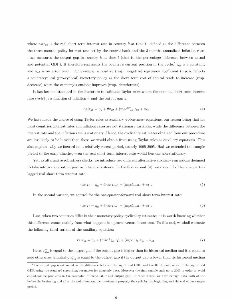
The histogram depicted in Figure 1 shows the results from the auxiliary regression (3). In particular it
shows that Great Britain and Sweden are the OECD countries with the most countercyclical real short term
interest rates over the period we consider. A natural explanation for this, is that both countries conduct
their own monetary policies, and through independent central banks. The least countercyclical among the
countries in our sample are Japan, Spain, Portugal and Finland. As for the latter three, they are all part
of the Euro area; moreover, all three are "small economies" in GDP terms compared to the Euro area as a
whole, therefore they are unlikely to have much in�uence on the European Central Bank�s policy; �nally,
in�ation is notoriously pro-cyclical in these countries, which in turn results in a real short term interest rate
which is higher in recessions than in booms. Japan is a separate story: there, the procyclicality of real short
term interest rates appears to be directly linked to a zero bound problem.
FIGURE 1 HERE
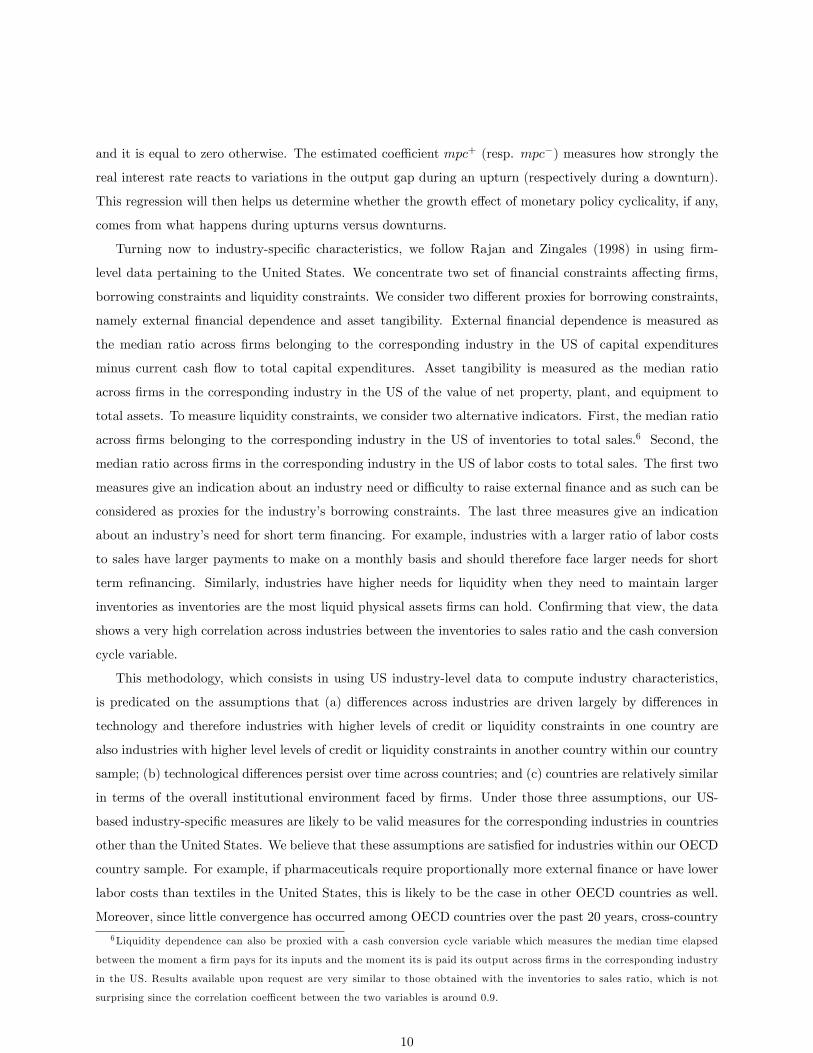
Alternatively we consider the results of the auxiliary regression (4) which provide the country-by-country
estimate for the output gap coe¢ cient in the Taylor rule (see �gure 2). The results are fairly comparable
to those from the previous estimation exercise. In particular, Great Britain and Sweden are still the most
counter-cyclical countries while Spain and Portugal are still (the most) procyclical countries.
FIGURE 2 HERE
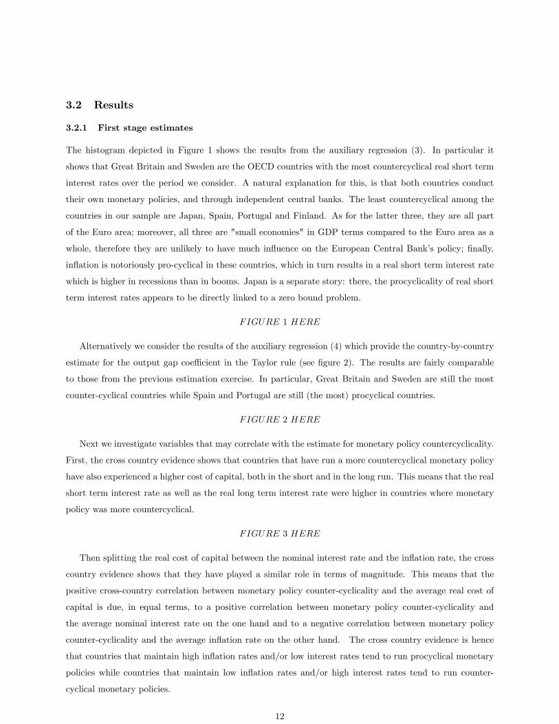
Next we investigate variables that may correlate with the estimate for monetary policy countercyclicality.
First, the cross country evidence shows that countries that have run a more countercyclical monetary policy
have also experienced a higher cost of capital, both in the short and in the long run. This means that the real
short term interest rate as well as the real long term interest rate were higher in countries where monetary
policy was more countercyclical.
FIGURE 3 HERE
Then splitting the real cost of capital between the nominal interest rate and the in�ation rate, the cross
country evidence shows that they have played a similar role in terms of magnitude. This means that the
positive cross-country correlation between monetary policy counter-cyclicality and the average real cost of
capital is due, in equal terms, to a positive correlation between monetary policy counter-cyclicality and
the average nominal interest rate on the one hand and to a negative correlation between monetary policy
counter-cyclicality and the average in�ation rate on the other hand. The cross country evidence is hence
that countries that maintain high in�ation rates and/or low interest rates tend to run procyclical monetary
policies while countries that maintain low in�ation rates and/or high interest rates tend to run counter-
cyclical monetary policies.
12
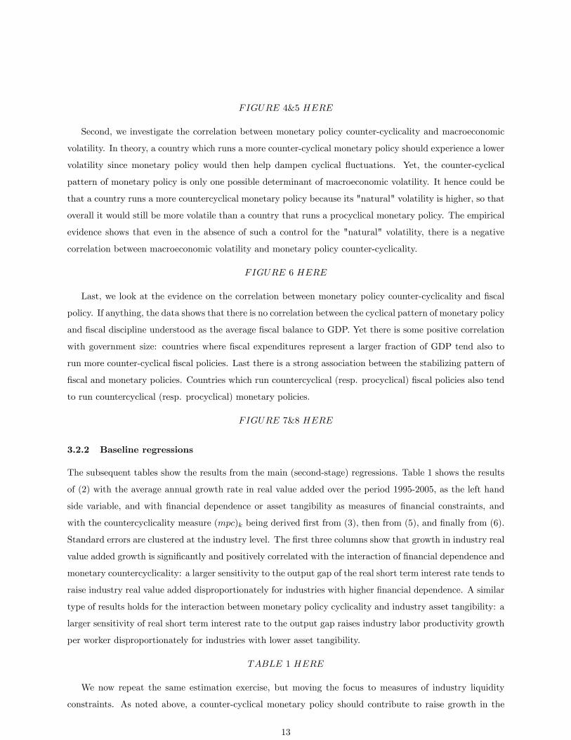
FIGURE 4&5 HERE
Second, we investigate the correlation between monetary policy counter-cyclicality and macroeconomic
volatility. In theory, a country which runs a more counter-cyclical monetary policy should experience a lower
volatility since monetary policy would then help dampen cyclical �uctuations. Yet, the counter-cyclical
pattern of monetary policy is only one possible determinant of macroeconomic volatility. It hence could be
that a country runs a more countercyclical monetary policy because its "natural" volatility is higher, so that
overall it would still be more volatile than a country that runs a procyclical monetary policy. The empirical
evidence shows that even in the absence of such a control for the "natural" volatility, there is a negative
correlation between macroeconomic volatility and monetary policy counter-cyclicality.
FIGURE 6 HERE
Last, we look at the evidence on the correlation between monetary policy counter-cyclicality and �scal
policy. If anything, the data shows that there is no correlation between the cyclical pattern of monetary policy
and �scal discipline understood as the average �scal balance to GDP. Yet there is some positive correlation
with government size: countries where �scal expenditures represent a larger fraction of GDP tend also to
run more counter-cyclical �scal policies. Last there is a strong association between the stabilizing pattern of
�scal and monetary policies. Countries which run countercyclical (resp. procyclical) �scal policies also tend
to run countercyclical (resp. procyclical) monetary policies.
FIGURE 7&8 HERE
3.2.2 Baseline regressions
The subsequent tables show the results from the main (second-stage) regressions. Table 1 shows the results
of (2) with the average annual growth rate in real value added over the period 1995-2005, as the left hand
side variable, and with �nancial dependence or asset tangibility as measures of �nancial constraints, and
with the countercyclicality measure (mpc)k being derived �rst from (3), then from (5), and �nally from (6).
Standard errors are clustered at the industry level. The �rst three columns show that growth in industry real
value added growth is signi�cantly and positively correlated with the interaction of �nancial dependence and
monetary countercyclicality: a larger sensitivity to the output gap of the real short term interest rate tends to
raise industry real value added disproportionately for industries with higher �nancial dependence. A similar
type of results holds for the interaction between monetary policy cyclicality and industry asset tangibility: a
larger sensitivity of real short term interest rate to the output gap raises industry labor productivity growth
per worker disproportionately for industries with lower asset tangibility.
TABLE 1 HERE
We now repeat the same estimation exercise, but moving the focus to measures of industry liquidity
constraints. As noted above, a counter-cyclical monetary policy should contribute to raise growth in the
13
sectors that are most liquidity dependent by easing the process of re�nancing. Indeed the empirical evidence
in Table 2 shows that for each of our two measures of liquidity constraints, the interaction of counter-
cyclical monetary policy and liquidity constraints does have a positive e¤ect on industry labor productivity
growth per worker. Moreover, as in the case of borrowing constraints, these results do not depend upon
the way in which monetary policy countercyclicality is estimated, in particular they are robust to taking
into account possible time persistence in the real short term interest rate. At this point it is worth making
two remarks. First the correlations between the two di¤erent measures of liquidity constraints is around
0.6, which means these two variables are not simply replicating a unique result. Moreover, the correlation
between indicators of borrowing constraint and liquidity constraint is also far from being one. It ranges
actually between 0.4 and 0.7 (when borrowing constraints are measured with external �nancial dependence,
correlations being opposite when using asset tangibility). Liquidity and borrowing constraints are therefore
two distinct channels through which monetary policy countercyclicality can a¤ect industry growth.
TABLE 2 HERE
Tables 3 and 4 below, replicate the same regression exercises as Table 1 and 2 respectively, but with
average annual growth in labor productivity per hour as the left hand side variable. We therefore aim at
understanding whether the positive e¤ect of countercyclical monetary policy on real value added growth
for �nancially/liquidity dependent industries comes from a true enhancement in productivity growth or if
it is simply re�ecting an increase in employment growth in which case, the growth e¤ect would simply be
related to factor accumulation.11 What Tables 3 and 4 show is that the interactions between �nancial or
liquidity constraints on the one hand and the countercyclicality of monetary policy on the other hand has a
signi�cantly positive e¤ect on labor productivity per hour growth.
TABLES 3 AND 4
3.2.3 Disentangling interest rate and in�ation cyclicality
Up to now we have focused on the real short term interest rate to assess whether monetary policy could
a¤ect growth through its cyclical component, which as has been noted above, is the di¤erence between the
nominal short term interest rate and in�ation. Hence a given cyclicality in the real short term interest rate
could uncover di¤erent patterns: a country where in�ation is less procyclical than another could well exhibit
a similar real short term interest rate cyclical pattern if the nominal interest rate is less countercyclical.
To determine whether it makes a di¤erence that real short term interest rate countercyclicality stems from
countercyclical nominal interest rates or from countercyclical in�ation rates, we have extended the analysis
11Looking moreover at productivity per hour is important to �lter out fact that the number of hours per worker tends to be
procyclical in upturns while acyclical in downturns. Looking just at the e¤ect of the interaction of �nancial constraints with
monetary policy countercyclicality on average growth in productivity per worker may therefore simply re�ect the (asymmetric)
e¤ect of that interaction on the number of hours per worker.
14
by separating these two e¤ects and estimating them separately. Columns i and ii in Table 5 typically show
that in�ation procyclicality -interacted with industry �nancial dependence- does not have any signi�cant
e¤ect beyond that embedded in the real short term countercyclicality. This means that what is important
for labor productivity growth is the cyclical pattern of the real short term interest rate, no matter whether
it comes from nominal interest rate or in�ation counter-cyclicality. Column iii in table 5 proposes another
way to answer this question since it runs a horse race between the cyclicality on nominal interest rates, for
given in�ation (like in a standard Taylor rule) and the cyclicality of in�ation (like in a standard Phillips
curve). If anything the empirical evidence is that these two e¤ects are of similar magnitude (i.e. there are
not statistically di¤erent from each other) which is indeed consistent with the view that what matters is the
extent to which the real short term interest rate is counter-cyclical, not the source of its counter-cyclicality.
The remaining columns in table 5 -which run a similar exercise using asset tangibility as an industry measure
of �nancial constraints- typically provide very consistent results in the sense that they con�rm the view that
countercyclical real short term interest rates do help foster productivity growth for industries with the least
tangible assets, irrespective of the source for countercyclicality (i.e. nominal interest vs. in�ation).
Next, table 6 provides the results of a similar analysis focusing now on industry measures of liquidity
dependence. Focusing on columns i-iii, results are somewhat di¤erent from those obtained in table 5 since
regressions show that in�ation countercyclicality is indeed the driving force for the e¤ect of real short term
interest rate countercyclicality on labor productivity growth. To be fair, the evidence is that nominal short
term interest rate countercyclicality does play a role. However it is either small (less than one fourth of the
e¤ect of in�ation countercyclicality, according to column i & ii) or not signi�cantly di¤erent from zero (column
iii). Actually this result is not unexpected. To the extent that �rms use their inventories as a collateral or
guarantee for credit, a procyclical in�ation will tend to reduce the value of inventories during downturns,
which is likely the time at which �rms most need to borrow. By contrast, a countercyclical in�ation will
raise the value of inventories during downturns, which will likely enhance �rms ability to borrow. It is hence
not surprising that the cyclicality of in�ation be key in determining the growth performance of industries
maintaining a high level for inventories.
3.2.4 Instrumenting monetary policy cyclicality
Up to now, the index for monetary policy cyclicality that is obtained from �rst stage regressions has been
considered as a variable that is observed, not estimated. Moreover it has also been considered exogenous to
industry growth (on the basis that an industry speci�c development cannot a¤ect the design of monetary
policy since the latter is concerned with the whole economy). Yet, in reality, monetary policy cyclicality is
estimated which means that we only know the �rst and second moments for the distribution of monetary
policy cyclicality for each country. Moreover monetary policy cyclicality may well be endogenous to industry
growth if monetary policy makers choose to run more countercyclical policies in economies where industries
face tighter �nancial or liquidity constraints. To overcome these two problems, we can rely on instrumental
15
variable estimations. Basically by taking variables that are known to be exogenous -in the sense that they
can a¤ect monetary policy cyclicality while monetary policy cyclicality cannot a¤ect them- we can get rid of
the possible endogeneity problem and the uncertainty around the estimate for monetary policy cyclicality. To
this end, we restrict the set of instruments to variables such as the legal origin of the country (French, English,
Scandinavian, and German), the population�s deep characteristics (share of Catholics in total population in
1980, share of Protestants in total population in 1980 and degree for ethnolinguistic fractionalization) and the
number of years since the country�s independence.12 Running the regressions with set of instruments actually
shows that there is a truly signi�cant e¤ect of the interaction between monetary policy counter-cyclicality and
industry �nancial or liquidity constraints on industry labor productivity growth. In other words, previous
results are not related to the existence of a reverse causality bias. Nor are they related to the uncertainty
around the estimates for monetary policy cyclicality. Actually a striking feature of the IV regressions is the
similarity in the estimated coe¢ cients when compared with those obtained in the OLS estimations, which
actually con�rms the prior that the cyclical pattern of monetary policy is likely to be exogenous to industry
labor productivity growth. A last remark has to do the test for the validity of instruments which is clearly
passed both in the case of industry �nancial constraints and in the case of liquidity constraints.13
TABLE 7&8 HERE
3.2.5 Competing stories and omitted variables
We have established that monetary policy cyclicality does enhance disproportionately the growth rate of
sectors that face tighter �nancial or liquidity constraints. Yet a concern is to which extent aren�t we picking
up other factors or stories when looking at the correlation between industry growth and the cyclicality of
�scal policy? The next four tables address this issue. First, it could be that a more countercyclical monetary
policy re�ects a higher degree of �nancial development in the country, and �nancial development in turn is
known to have a positive e¤ect on growth, particularly for industries that are more dependent on external
�nance (Rajan and Zingales, 1998). Second, the higher in�ation, the higher the cost of capital, which in turn
should penalize more �nancially constrained sectors more in the absence of suitable macroeconomic policies;
at the same time, higher in�ation is likely to a¤ect the government�s ability to implement countercyclical
monetary policies. Third, monetary countercyclicality may also be related to the size of government or its
degree of �scal discipline.
Table 5 performs horse-races between the e¤ect of the interaction between asset tangibility and the
countercyclicality of monetary policy and the interaction of asset tangibility with measures of �nancial
development, in�ation, and government size/budgetary discipline, on average growth in labor productivity
12Following Persson, Tabellini and Trebbi (2003), the independence year is set at 1748 for countries that have never been
colonized.13Note that in the regressions incorporating liquidity constraints, there may a weak instruments problem, which can solved
by restricting the set of instruments used for estimation. The point here is to show that a unique set of instrument can go a long
way to dealing with potential endogeneity and measurement error issues with a set of relatively di¤erent industry characteristics.
16
per hour. The �rst column shows that when controlling for the interaction between asset tangibility and
in�ation in the second stage regression with the growth of labor productivity per hour as left hand side
variable, the coe¢ cient for the interaction between asset tangibility and countercyclical monetary policy,
remains una¤ected. Moreover, the coe¢ cient for in�ation interacted with countercyclical monetary policy
is not signi�cant. The next four columns control for asset tangibility interacted with di¤erent measures
of �nancial development. Once again, adding these controls leaves the magnitude and signi�cance of the
interaction term between asset tangibility and monetary countercyclicality una¤ected. The next two columns
control for the interaction between asset tangibility and the average government debt and average government
expenditure to GDP ratios (two measures of government size), and the last column controls for the interaction
between asset tangibility and the average government surplus to GDP ratio (our measure of �scal discipline):
again, controlling for these interactions does not a¤ect the magnitude and signi�cance of the interaction
coe¢ cient between asset tangibility and monetary countercyclicality.
TABLE 9 HERE
Table 6 repeats the same exercise, but using external �nancial dependence as the measure of �nancial
constraint. The basic conclusions are the same as in the previous Table, namely that controlling for the
interaction between �nancial dependence and in�ation, �nancial development of government size/budgetary
discipline does not impact on the magnitude and signi�cance of the interaction term between �nancial
dependence and monetary countercyclicality. Note however the importance and signi�cance of the interaction
term between in�ation and �nancial dependence in this regression, which goes in the direction predicted
above.
TABLE 10 HERE
Tables 7 and 8 are more interesting: they perform the same horse race exercises as the previous two tables,
but using liquidity constraint measures -labor costs to sales and inventories to sales ratios respectively- as
�nancial interactors. AS one can see in these two tables, the interaction between these two measures of
liquidity constraints and the countercyclicality of monetary policy overwhelms the interaction of the same
liquidity constraints measures with in�ation, �nancial development and government size/budgetary discipline
in the sense that none of these other interactions ever comes out signi�cant. This in turn suggests that
monetary policy countercyclicality is of paramount importance especially for those sectors that are more
prone to be liquidity constrained.
TABLE 11 AND 12 HERE
These results do not imply that in�ation, �nancial development or government size/�scal discipline do
not matter for industry growth in industries that are more liquidity constrained. It rather means that if
they matter, it is primarily through their e¤ects on the government�s ability to implement countercyclical
monetary policies.
17
3.2.6 Upturns versus downturns, high-tech versus low-tech sectors
Table 9 runs the second stage regression (2), separately for country-years where the output gap is respect-
ively below and above its median value over the whole period for the corresponding country (thus we look
separately at upturns and downturns). The interaction e¤ects between �nancial constraints and monetary
countercyclicality are always signi�cant in downturns, no matter if we use �nancial dependence, asset tan-
gibility, the labor to sales ratio or the inventories to sales ratio. Moreover, except when asset tangibility is
used as the �nancial interactor, the interaction between �nancial constraints and monetary countercyclical-
ity tend to be more signi�cant in slumps than in booms (when asset tangibility as the �nancial interactor,
the interaction coe¢ cient is comparable in upturns and downturns). This in turn is consistent with the
idea that more countercyclical real short term interest rates have a more signi�cant e¤ect on average labor
productivity growth of industries during downturns when �nancial constraints are more likely to be binding.
TABLE 13 HERE
Table 10 runs the second stage regression (2) separately for high-tech and for low-tech industries. Except
when asset tangibility is used as the measure of �nancial constraint, the interaction term between �nancial
constraints and monetary policy countercyclicality, is slightly higher for high-tech industries. Why does the
opposite conclusion obtain when using asset tangibility as the �nancial interactor? Our tentative explanation
is that the distinction between high-tech and low-tech sectors is collinear with asset tangibility: high-tech
sectors typically show lower degree of asset tangibility than low-tech sectors. This in turn suggests that
what the interaction term between asset tangibility and monetary countercyclicality policy captures once we
control for high- versus low-tech sectors, is in fact essentially a country �xed e¤ect.
TABLE 14 HERE
Tables 11 and 12 combine the breakdowns between upturns and downturns and between high- and low-
tech sectors. Table 11 considers credit constraints measures (�nancial dependence and asset tangibility) as
�nancial interactors, whereas Table 12 looks at liquidity constraint measures (inventories to GDP and labor
costs to GDP ratios) as �nancial interactors. The most interesting �nding from these two tables, is that
while in downturns both, high-tech and low-tech sectors seem to bene�t from more countercyclical monetary
policies, i.e from lower real short-run interest rates in downturns, in upturns it is the high-tech sectors which
bene�t most from more countercyclical monetary policy, i.e from higher short-run interest rates. In other
words, there is a cost of having low short-run interest rates in booms, namely that of allocating to much
capital to low-tech sectors at the expense of high-tech sectors.
TABLE 15 AND 16 HERE
18

4 Conclusion
In this paper we have developed a simple framework to look at how the interaction between the cyclic-
ality of (short-run-) interest rate policy and �rms�credit or liquidity constraints, a¤ects �rms� long-term
growth-enhancing investments. Three main predictions came out of our mode, namely: (i) the more credit-
constrained an industry, the more growth in that industry bene�ts from more countercyclical interest rates;
(ii) the more liquidity-constrained an industry, the more growth in that industry bene�ts from more coun-
tercyclical interest rates; (iii) the growth enhancing e¤ect of countercyclical interest rate policies in more
credit- or liquidity-constrained sectors, is more signi�cant in downturns than in upturns. Then, we have suc-
cessfully confronted these predictions to quarterly cross-industry, cross-country OECD data over the period
1995-2005.
The approach and analysis in this paper could be extended in several interesting directions. First, one
could revisit the costs and bene�ts of monetary unions, i.e of the potential credibility gains from joining
the union versus the potential costs in terms of the reduced ability to pursue countercyclical monetary
policies. Here, we think for example of countries like Greece or Spain where interest rates went down after
these countries joined the Eurozone but which at the same time were becoming subject to cyclical monetary
policies which were no longer set with the primary objective of maximizing investment and growth in these
countries.
Second, one could look at the interplay between cyclical monetary policy and cyclical �scal policy: are
those substitutes or complements?
Third, one could embed our analysis in this paper into a broader framework where interest rate policy
would also a¤ect the extent of collective moral hazard among banks as in Farhi and Tirole (2010). Lowering
interest rates in a downturn would then have the counteracting e¤ect of encouraging excessive short-term
debt borrowing by banks.
Finally, one could look deeper into the potential ine¢ ciencies of setting low interest rates during upturns.
In particular, to which extent can that lead to sectoral misallocation of funds between high-tech and low-tech
sectors, and how do the corresponding allocative ine¢ ciencies compare to the ine¢ ciency associated with
excessive risk-taking by banks? All these extensions await further research.
References
[1] Acemoglu, D, Johnson, S, Robinson, J, and Y. Thaicharoen (2003), �Institutional Causes, Macroeco-
nomic Symptoms: Volatility, Crises, and Growth�, Journal of Monetary Economics, 50, 49-123.
[2] Aghion, P, Bacchetta, P., Ranciere, R., and K. Rogo¤ (2006), �Exchange Rate Volatility and Productiv-
ity Growth: The Role of Financial Development�, NBER Working Paper No 12117.
19

[3] Aghion, P, Hemous, D, and E. Kharroubi (2009), "Cyclical Fiscal Policy, Credit Constraints, and
Industry Growth", mimeo Harvard.
[4] Beck, T, Demirgüç-Kunt, A, and R. Levine (2000), "A New Database on Financial Development and
Structure," World Bank Economic Review 14, 597-605.
[5] Bernanke, B, and M. Gertler (1995), "Inside the Black Box: The Credit Channel of Monetary Policy
Transmission", Journal of Economic Perspectives, 9: 27-48
[6] Braun, M, and B. Larrain (2005), "Finance and the Business Cycle: International, Inter-Industry Evid-
ence", The Jounral of Finance, vol. 60(3), 1097-1128
[7] Easterly, W. (2005), �National Policies and Economic Growth: A Reappraisal�, Chapter 15 in Handbook
of Economic Growth, P. Aghion and S. Durlauf eds.
[8] Farhi, E, and J. Tirole (2010), "Collective Moral Hazard, Maturity Mismatch, and Systemic Bailouts",
forthcoming in the American Economic Review.
[9] Holmstrom, B, and J. Tirole (1998), �Private and Public Supply of liquidity� Journal of Political
Economy, vol. 106(1), 1-40.
[10] Kaminski, G, Reinhart, C, and C. Végh, (2004) �When it Rains it Pours: Procyclical Capital Flows
and Macroeconomic Policies,�NBER Macroeconomics Annual.
[11] Raddatz, C. (2006), �Liquidity needs and vulnerability to �nancial underdevelopment,� Journal of
Financial Economics vol. 80, 677-722.
[12] Rajan, R, and L. Zingales (1998), �Financial dependence and Growth�American Economic Review,
vol. 88, 559-586.
[13] Ramey, G, and V. Ramey (1995), �Cross-Country Evidence on the Link between Volatility and Growth�,
American Economic Review, 85 (5), 1138-51
[14] Ramey, V. (2008), �Identifying Government Spending Shocks: It�s All in the Timing", mimeo
[15] Romer, C, and D. Romer (2007), "The macroeconomic e¤ects of tax changes: estimates based on a new
measure of �scal shocks", NBER Working Paper No. 13264.
[16] Woodford, M (1990), "Public Debt as Private Liquidity", American Economic Review, 80, 382-388
20
5 Appendix
Assumption 3 (high return)
��� (�1 � �0)RG1 + (1� �) (�1 � �0) + �GRG1 + (1� �)
��G � 1
�RG1�
1� � �0R0� �(1� �) �0
R0RG1+ (1� �) (1� �) q
�1��BR0
� �0R0RB
1
�+
(1� �)�� (�1 � �0)RB1 + (1� �) (�1 � �0) + ��BRB1
�1� � �0
R0� �(1� �) �0
R0RG1+ (1� �) (1� �) q
�1��BR0
� �0R0RB
1
� > R0(�RG1 + (1� �)RB1 ):Assumption 4 (demand for liquidity):
(�1 � �0)1� �0
RB1
R0q���� (�1 � �0)RG1 + (1� �) (�1 � �0) + �GRG1 + (1� �)
��G � 1
�RG1�
1� � �0R0� �(1� �) �0
R0RG1
+
(1� �)�� (�1 � �0)RB1 + (1� �) (�1 � �0) x+�
B
1� �0RB1
+ ��BRB1
�1� � �0
R0� �(1� �) �0
R0RG1
:
Proof that Assumption 4 implies that entrepreneurs hoard enough liquidity to weather liquidity
shocks. The entrepreneur therefore maximizes over x 2 [0; 1� �0=RB1 � �B ] :
A��� (�1 � �0)RG1 + (1� �) (�1 � �0) + �GRG1 + (1� �)
��G � 1
�RG1�
1� � �0R0� �(1� �) �0
R0RG1+ (1� �) (1� �) qxR0
+
(1� �)�� (�1 � �0)RB1 + (1� �) (�1 � �0) x+�
B
1� �0RB1
+ ��BRB1
�1� � �0
R0� �(1� �) �0
R0RG1+ (1� �) (1� �) qxR0
:
This expression is increasing in x if and only if Assumption 4 holds.
Proof that Assumption 3 implies that entrepreneurs invest all their net worth in their project.
By investing in his own project, the entrepreneur gets an expected return of:
��� (�1 � �0)RG1 + (1� �) (�1 � �0) + �GRG1 + (1� �)
��G � 1
�RG1�
1� � �0R0� �(1� �) �0
R0RG1+ (1� �) (1� �) q
�1��BR0
� �0R0RB
1
�+
(1� �)�� (�1 � �0)RB1 + (1� �) (�1 � �0) + ��BRB1
�1� � �0
R0� �(1� �) �0
R0RG1+ (1� �) (1� �) q
�1��BR0
� �0R0RB
1
�which Assumption guarantees is greater than the return he gets by investing his net worth at the risk-free
rate and rolling it over.
21
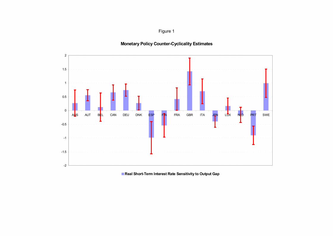
Figure 1
Monetary Policy Counter-Cyclicality Estimates
-2
-1.5
-1
-0.5
0
0.5
1
1.5
2
AUS AUT BEL CAN DEU DNK ESP FIN FRA GBR ITA JPN LUX NLD PRT SWE
Real Short-Term Interest Rate Sensitivity to Output Gap
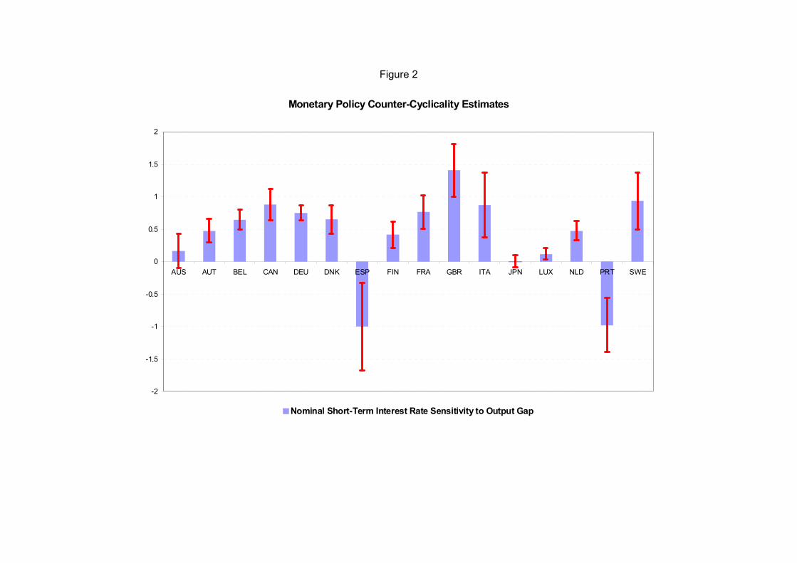
Figure 2
Monetary Policy Counter-Cyclicality Estimates
-2
-1.5
-1
-0.5
0
0.5
1
1.5
2
AUS AUT BEL CAN DEU DNK ESP FIN FRA GBR ITA JPN LUX NLD PRT SWE
Nominal Short-Term Interest Rate Sensitivity to Output Gap
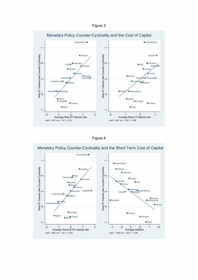
Figure 3
Ireland Netherlands
Japan
Spain
Luxembourg
Portugal
Belgium
Austria
Finland
Denmark
Italy Germany
France
Sweden
Canada
Greece
Great-Britain
Australia
-1-.5
0.5
1R
eal S
T in
tere
st ra
te C
ount
er-C
yclic
ality
-2 -1 0 1 2Average Real ST interest rate
coef = .437, se = .121, t = 3.6
Ireland
Japan
Greece
Netherlands
Spain
Luxembourg
Portugal
Italy
Belgium
Austria
Great-Britain
Denmark
Germany
France
Finland
Australia
Sweden
Canada
-1-.5
0.5
1R
eal S
T in
tere
st ra
te C
ount
er-C
yclic
ality
-2 -1 0 1Average Real LT interest rate
coef = .401, se = .157, t = 2.56
Monetary Policy Counter-Cyclicality and the Cost of Capital
Figure 4
Japan
NetherlandsIreland
Luxembourg
Spain
Belgium
Portugal
AustriaGreece
Finland
Denmark
GermanyItaly
France
Sweden
Canada
Great-Britain
Australia
-1-.5
0.5
1R
eal S
T in
tere
st ra
te C
ount
er-C
yclic
ality
-2 -1 0 1 2Average Nominal ST interest rate
coef = .462, se = .131, t = 3.52
Australia
Great-Britain
Sweden
CanadaFrance
Germany
Japan
Finland
Denmark
Austria
Belgium
Italy
Luxembourg
Portugal
Spain
NetherlandsGreece
Ireland
-1-.5
0.5
1R
eal S
T in
tere
st ra
te C
ount
er-C
yclic
ality
-1 -.5 0 .5 1 1.5Average Inflation
coef = -.446, se = .152, t = -2.94
Monetary Policy Counter-Cyclicality and the Short Term Cost of Capital
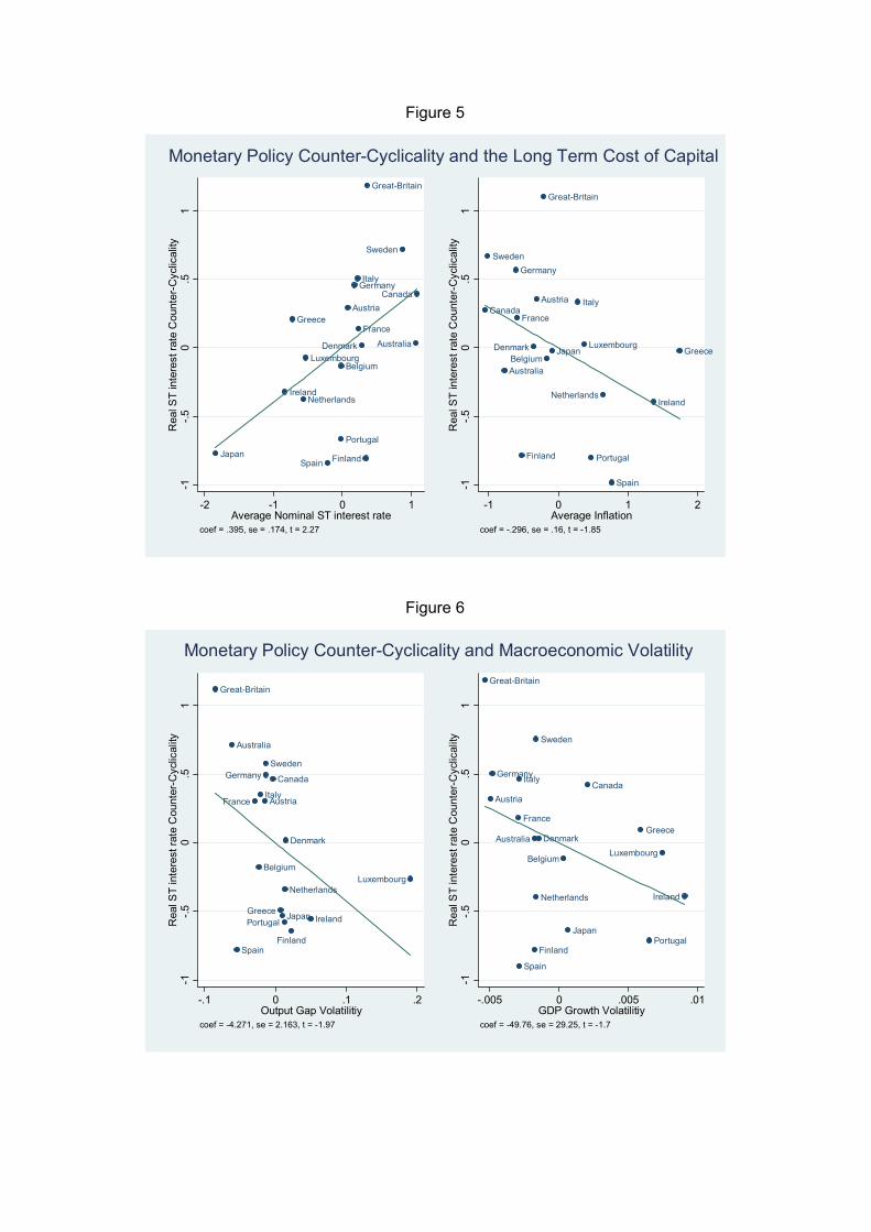
Figure 5
Japan
Ireland
Greece
Netherlands
Luxembourg
Spain
Portugal
Belgium
Austria
GermanyItaly
France
Denmark
Finland
Great-Britain
Sweden
Australia
Canada
-1-.5
0.5
1R
eal S
T in
tere
st ra
te C
ount
er-C
yclic
ality
-2 -1 0 1Average Nominal ST interest rate
coef = .395, se = .174, t = 2.27
Canada
Sweden
Australia
Germany
France
Finland
Denmark
Austria
Great-Britain
BelgiumJapan
Italy
Luxembourg
Portugal
Netherlands
Spain
Ireland
Greece
-1-.5
0.5
1R
eal S
T in
tere
st ra
te C
ount
er-C
yclic
ality
-1 0 1 2Average Inflation
coef = -.296, se = .16, t = -1.85
Monetary Policy Counter-Cyclicality and the Long Term Cost of Capital
Figure 6
Great-Britain
Australia
Spain
France
Belgium
ItalyAustria
GermanySweden
Canada
Greece JapanPortugal
Netherlands
Denmark
Finland
Ireland
Luxembourg
-1-.5
0.5
1R
eal S
T in
tere
st ra
te C
ount
er-C
yclic
ality
-.1 0 .1 .2Output Gap Volatilitiy
coef = -4.271, se = 2.163, t = -1.97
Great-Britain
Austria
Germany
France
Italy
Spain
Finland
Australia
Sweden
Netherlands
Denmark
Belgium
Japan
Canada
Greece
Portugal
Luxembourg
Ireland
-1-.5
0.5
1R
eal S
T in
tere
st ra
te C
ount
er-C
yclic
ality
-.005 0 .005 .01GDP Growth Volatilitiy
coef = -49.76, se = 29.25, t = -1.7
Monetary Policy Counter-Cyclicality and Macroeconomic Volatility
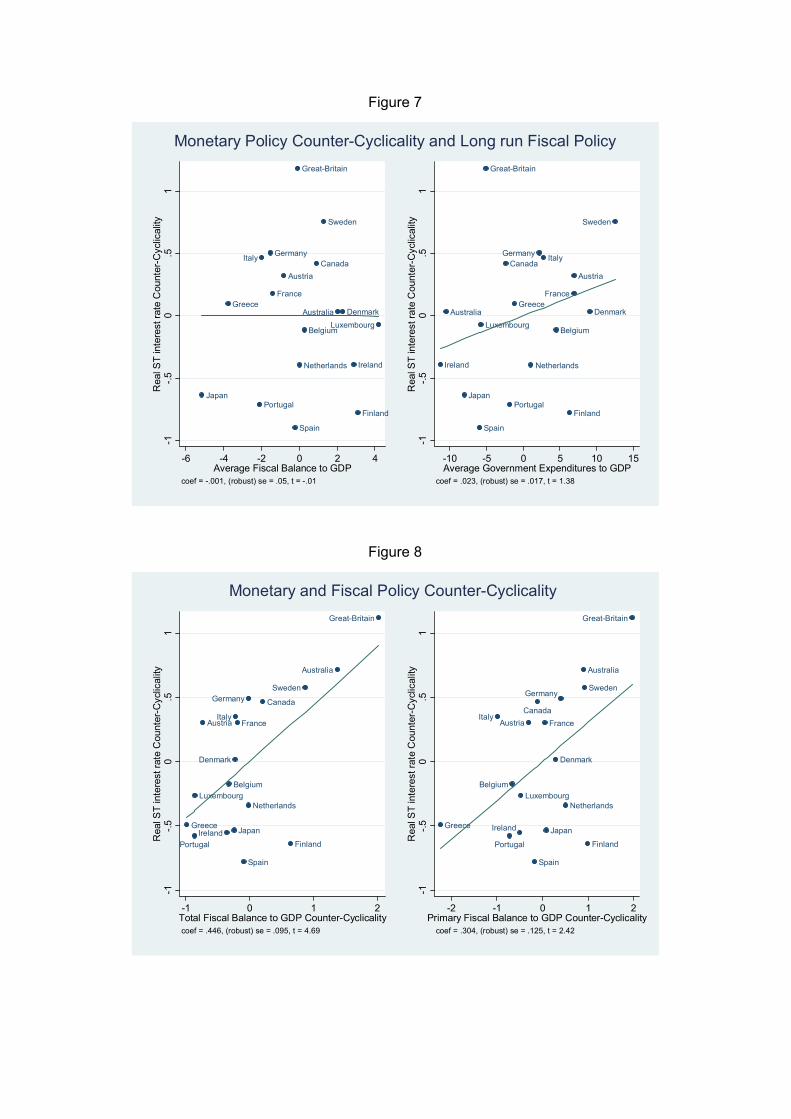
Figure 7
Japan
Greece
Portugal
Italy Germany
France
Austria
Spain
Great-Britain
Netherlands
Belgium
Canada
Sweden
Australia Denmark
Ireland
Finland
Luxembourg
-1-.5
0.5
1R
eal S
T in
tere
st ra
te C
ount
er-C
yclic
ality
-6 -4 -2 0 2 4Average Fiscal Balance to GDP
coef = -.001, (robust) se = .05, t = -.01
Ireland
Australia
Japan
Spain
Luxembourg
Great-Britain
Canada
Portugal
Greece
Netherlands
Germany Italy
Belgium
Finland
France
Austria
Denmark
Sweden
-1-.5
0.5
1R
eal S
T in
tere
st ra
te C
ount
er-C
yclic
ality
-10 -5 0 5 10 15Average Government Expenditures to GDP
coef = .023, (robust) se = .017, t = 1.38
Monetary Policy Counter-Cyclicality and Long run Fiscal Policy
Figure 8
Greece
Portugal
Luxembourg
Austria
Ireland
Belgium
Japan
Denmark
ItalyFrance
Spain
Germany
Netherlands
Canada
Finland
Sweden
Australia
Great-Britain
-1-.5
0.5
1R
eal S
T in
tere
st ra
te C
ount
er-C
yclic
ality
-1 0 1 2Total Fiscal Balance to GDP Counter-Cyclicalitycoef = .446, (robust) se = .095, t = 4.69
Greece
Italy
Portugal
Belgium
Ireland
Luxembourg
Austria
Spain
CanadaFrance
Japan
Denmark
Germany
Netherlands
Australia
Sweden
Finland
Great-Britain
-1-.5
0.5
1R
eal S
T in
tere
st ra
te C
ount
er-C
yclic
ality
-2 -1 0 1 2Primary Fiscal Balance to GDP Counter-Cyclicality
coef = .304, (robust) se = .125, t = 2.42
Monetary and Fiscal Policy Counter-Cyclicality
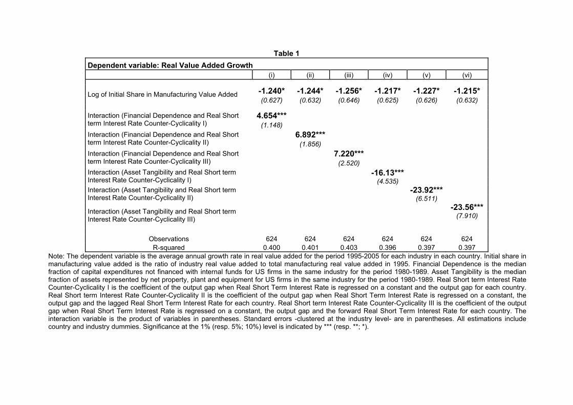
Table 1 Dependent variable: Real Value Added Growth (i) (ii) (iii) (iv) (v) (vi)
-1.240* -1.244* -1.256* -1.217* -1.227* -1.215* Log of Initial Share in Manufacturing Value Added (0.627) (0.632) (0.646) (0.625) (0.626) (0.632)
4.654*** Interaction (Financial Dependence and Real Short term Interest Rate Counter-Cyclicality I) (1.148)
6.892*** Interaction (Financial Dependence and Real Short term Interest Rate Counter-Cyclicality II) (1.856)
7.220*** Interaction (Financial Dependence and Real Short term Interest Rate Counter-Cyclicality III) (2.520)
-16.13*** Interaction (Asset Tangibility and Real Short term Interest Rate Counter-Cyclicality I) (4.535)
-23.92*** Interaction (Asset Tangibility and Real Short term Interest Rate Counter-Cyclicality II) (6.511)
-23.56*** (7.910) Interaction (Asset Tangibility and Real Short term
Interest Rate Counter-Cyclicality III)
Observations 624 624 624 624 624 624 R-squared 0.400 0.401 0.403 0.396 0.397 0.397
Note: The dependent variable is the average annual growth rate in real value added for the period 1995-2005 for each industry in each country. Initial share in manufacturing value added is the ratio of industry real value added to total manufacturing real value added in 1995. Financial Dependence is the median fraction of capital expenditures not financed with internal funds for US firms in the same industry for the period 1980-1989. Asset Tangibility is the median fraction of assets represented by net property, plant and equipment for US firms in the same industry for the period 1980-1989. Real Short term Interest Rate Counter-Cyclicality I is the coefficient of the output gap when Real Short Term Interest Rate is regressed on a constant and the output gap for each country. Real Short term Interest Rate Counter-Cyclicality II is the coefficient of the output gap when Real Short Term Interest Rate is regressed on a constant, the output gap and the lagged Real Short Term Interest Rate for each country. Real Short term Interest Rate Counter-Cyclicality III is the coefficient of the output gap when Real Short Term Interest Rate is regressed on a constant, the output gap and the forward Real Short Term Interest Rate for each country. The interaction variable is the product of variables in parentheses. Standard errors -clustered at the industry level- are in parentheses. All estimations include country and industry dummies. Significance at the 1% (resp. 5%; 10%) level is indicated by *** (resp. **; *).
Table 2 Dependent variable: Real Value Added Growth (i) (ii) (iii) (iv) (v) (vi)
-1.198* -1.211* -1.201* -1.191* -1.188* -1.184* Log of Initial Share in Manufacturing Value Added (0.634) (0.637) (0.643) (0.629) (0.631) (0.641)
26.49** Interaction (Inventories to Sales and Real Short term Interest Rate Counter-Cyclicality I) (10.66)
40.82** Interaction (Inventories to Sales and Real Short term Interest Rate Counter-Cyclicality II) (15.84)
46.04** Interaction (Inventories to Sales and Real Short term Interest Rate Counter-Cyclicality III) (17.58)
16.96*** Interaction (Labor Costs to Sales and Real Short term Interest Rate Counter-Cyclicality I) (5.374)
25.45*** Interaction (Labor Costs to Sales and Real Short term Interest Rate Counter-Cyclicality II) (8.076)
21.93* (11.07)
Interaction (Labor Costs to Sales and Real Short term Interest Rate Counter-Cyclicality III)
Observations 624 624 624 624 624 624 R-squared 0.393 0.394 0.396 0.395 0.395 0.394
Note: The dependent variable is the average annual growth rate in real value added for the period 1995-2005 for each industry in each country. Initial share in manufacturing value added is the ratio of industry real value added to total manufacturing real value added in 1995. Inventories to Sales is the median ratio of total inventories over annual sales for US firms in the same industry for the period 1980-1989. Labor Costs to Sales is the median ratio of labor costs to shipments for US firms in the same industry for the period 1980-1989. Real Short term Interest Rate Counter-Cyclicality I is the coefficient of the output gap when Real Short Term Interest Rate is regressed on a constant and the output gap for each country. Real Short term Interest Rate Counter-Cyclicality II is the coefficient of the output gap when Real Short Term Interest Rate is regressed on a constant, the output gap and the lagged Real Short Term Interest Rate for each country. Real Short term Interest Rate Counter-Cyclicality III is the coefficient of the output gap when Real Short Term Interest Rate is regressed on a constant, the output gap and the forward Real Short Term Interest Rate for each country. The interaction variable is the product of variables in parentheses. Standard errors -clustered at the industry level- are in parentheses. All estimations include country and industry dummies. Significance at the 1% (resp. 5%; 10%) level is indicated by *** (resp. **; *).

Table 3 Dependent variable: Labor Productivity per hour Growth (i) (ii) (iii) (iv) (v) (vi)
-3.528*** -3.599*** -3.574*** -3.544*** -3.578*** -3.584***Log of Initial Relative Labor Productivity (0.877) (0.904) (0.91) (0.888) (0.91) (0.907)
3.713*** Interaction (Financial Dependence and Real Short term Interest Rate Counter-Cyclicality I) (1.224)
5.692** Interaction (Financial Dependence and Real Short term Interest Rate Counter-Cyclicality II) (2.248)
5.994** Interaction (Financial Dependence and Real Short term Interest Rate Counter-Cyclicality III) (2.643)
-12.98*** Interaction (Asset Tangibility and Real Short term Interest Rate Counter-Cyclicality I) (4.095)
-20.16*** Interaction (Asset Tangibility and Real Short term Interest Rate Counter-Cyclicality II) (6.862)
-21.02*** (6.916)
Interaction (Asset Tangibility and Real Short term Interest Rate Counter-Cyclicality III)
Observations 624 624 624 624 624 624 R-squared 0.364 0.365 0.367 0.36 0.362 0.363
Note: The dependent variable is the average annual growth rate in labor productivity per hour for the period 1995-2005 for each industry in each country. Initial Relative Labor Productivity is the ratio of industry labor productivity per hour to total manufacturing labor productivity per hour in 1995. Financial Dependence is the median fraction of capital expenditures not financed with internal funds for US firms in the same industry for the period 1980-1989. Asset Tangibility is the median fraction of assets represented by net property, plant and equipment for US firms in the same industry for the period 1980-1989. Real Short term Interest Rate Counter-Cyclicality I is the coefficient of the output gap when Real Short Term Interest Rate is regressed on a constant and the output gap for each country. Real Short term Interest Rate Counter-Cyclicality II is the coefficient of the output gap when Real Short Term Interest Rate is regressed on a constant, the output gap and the lagged Real Short Term Interest Rate for each country. Real Short term Interest Rate Counter-Cyclicality III is the coefficient of the output gap when Real Short Term Interest Rate is regressed on a constant, the output gap and the forward Real Short Term Interest Rate for each country. The interaction variable is the product of variables in parentheses. Standard errors -clustered at the industry level- are in parentheses. All estimations include country and industry dummies. Significance at the 1% (resp. 5%; 10%) level is indicated by *** (resp. **; *).
Table 4 Dependent variable: Labor Productivity per hour Growth (i) (ii) (iii) (iv) (v) (vi)
-3.677*** -3.721*** -3.743*** -3.589*** -3.594*** -3.586***Log of Initial Relative Labor Productivity (0.884) (0.905) (0.909) (0.864) (0.88) (0.866)
29.48*** Interaction (Inventories to Sales and Real Short term Interest Rate Counter-Cyclicality I) (8.774)
47.40*** Interaction (Inventories to Sales and Real Short term Interest Rate Counter-Cyclicality II) (13.87)
52.74*** Interaction (Inventories to Sales and Real Short term Interest Rate Counter-Cyclicality III) (14.56)
17.42*** Interaction (Labor Costs to Sales and Real Short term Interest Rate Counter-Cyclicality I) (4.244)
28.03*** Interaction (Labor Costs to Sales and Real Short term Interest Rate Counter-Cyclicality II) (7.143)
25.16*** Interaction (Labor Costs to Sales and Real Short term Interest Rate Counter-Cyclicality III) (9.145)
Observations 624 624 624 624 624 624 R-squared 0.362 0.365 0.368 0.363 0.365 0.363
Note: The dependent variable is the average annual growth rate in labor productivity per hour for the period 1995-2005 for each industry in each country. Initial Relative Labor Productivity is the ratio of industry labor productivity per hour to total manufacturing labor productivity per hour in 1995. Inventories to Sales is the median ratio of total inventories over annual sales for US firms in the same industry for the period 1980-1989. Labor Costs to Sales is the median ratio of labor costs to shipments for US firms in the same industry for the period 1980-1989. Real Short term Interest Rate Counter-Cyclicality I is the coefficient of the output gap when Real Short Term Interest Rate is regressed on a constant and the output gap for each country. Real Short term Interest Rate Counter-Cyclicality II is the coefficient of the output gap when Real Short Term Interest Rate is regressed on a constant, the output gap and the lagged Real Short Term Interest Rate for each country. Real Short term Interest Rate Counter-Cyclicality III is the coefficient of the output gap when Real Short Term Interest Rate is regressed on a constant, the output gap and the forward Real Short Term Interest Rate for each country. The interaction variable is the product of variables in parentheses. Standard errors -clustered at the industry level- are in parentheses. All estimations include country and industry dummies. Significance at the 1% (resp. 5%; 10%) level is indicated by *** (resp. **; *).
Table 5 Dependent variable: Labor Productivity per hour Growth (i) (ii) (iii) (iv) (v) (vi)
-3.561*** -3.590*** -3.586*** -3.532*** -3.536*** -3.556***Log of Initial Relative Labor Productivity (0.896) (0.901) (0.902) (0.886) (0.894) (0.896)
3.023*** 2.747** Interaction (Financial Dependence and Real Short term Interest Rate Counter-Cyclicality) (1.061) (1.063)
3.199*** Interaction (Financial Dependence and Taylor Rule Counter-Cyclicality) (1.122)
-2.965 Interaction (Financial Dependence and Inflation Pro-Cyclicality I) (2.585)
-2.967 -5.204** Interaction (Financial Dependence and Inflation Pro-Cyclicality II) (1.883) (2.079)
-11.55*** -10.60** Interaction (Asset Tangibility and Real Short term Interest Rate Counter-Cyclicality) (4.241) (3.986)
-11.97***Interaction (Asset Tangibility and Taylor Rule Counter-Cyclicality) (3.962)
5.755 Interaction (Asset Tangibility and Inflation Pro-Cyclicality I) (9.740)
6.858 15.49* (8.812) (8.194)
Interaction (Asset Tangibility and Inflation Pro-Cyclicality II)
Observations 624 624 624 624 624 624 R-squared 0.365 0.365 0.367 0.360 0.361 0.362
Note: The dependent variable is the average annual growth rate in labor productivity per hour for the period 1995-2005 for each industry in each country. Initial Relative Labor Productivity is the ratio of industry labor productivity per hour to total manufacturing labor productivity per hour in 1995. Financial Dependence is the median fraction of capital expenditures not financed with internal funds for US firms in the same industry for the period 1980-1989. Asset Tangibility is the median fraction of assets represented by net property, plant and equipment for US firms in the same industry for the period 1980-1989. Real Short term Interest Rate Counter-Cyclicality is the coefficient of the output gap when Real Short Term Interest Rate is regressed on a constant and the output gap for each country. Taylor Rule Counter-Cyclicality is the coefficient of the output gap when the Nominal Short Term Interest Rate is regressed on a constant, the output gap and inflation for each country. Inflation Pro-Cyclicality I (resp. II) is the coefficient of the output gap when Inflation is regressed on a constant, the output gap (resp. and lagged Inflation). The interaction variable is the product of variables in parentheses. Standard errors -clustered at the industry level- are in parentheses. All estimations include country and industry dummies. Significance at the 1% (resp. 5%; 10%) level is indicated by *** (resp. **; *).
Table 6 Dependent variable: Labor Productivity per hour Growth (i) (ii) (iii) (iv) (v) (vi)
-3.594*** -3.600*** -3.601*** -3.630*** -3.631*** -3.649***Log of Initial Relative Labor Productivity (0.869) (0.875) (0.876) (0.884) (0.891) (0.895)
19.33* 16.82* Interaction (Inventories to Sales and Real Short term Interest Rate Counter-Cyclicality) (9.933) (9.733)
17.36 Interaction (Inventories to Sales and Taylor Rule Counter-Cyclicality) (10.46)
-41.97** Interaction (Inventories to Sales and Inflation Pro-Cyclicality I) (20.50)
-37.47** -51.39*** Interaction (Inventories to Sales and Inflation Pro-Cyclicality II) (16.19) (14.09)
15.24*** 12.14** Interaction (Labor costs to Sales and Real Short term Interest Rate Counter-Cyclicality) (4.911) (4.807)
13.19** Interaction (Labor costs to Sales and Taylor Rule Counter-Cyclicality) (5.031)
-9.159 Interaction (Labor costs to Sales and Inflation Pro-Cyclicality I) (15.26)
-15.90 -25.87*** (10.51) (9.102)
Interaction (Labor costs to Sales and Inflation Pro-Cyclicality II)
Observations 624 624 624 624 624 624 R-squared 0.366 0.366 0.366 0.363 0.364 0.365
Note: The dependent variable is the average annual growth rate in labor productivity per hour for the period 1995-2005 for each industry in each country. Initial Relative Labor Productivity is the ratio of industry labor productivity per hour to total manufacturing labor productivity per hour in 1995. Inventories to Sales is the median ratio of total inventories over annual sales for US firms in the same industry for the period 1980-1989. Labor Costs to Sales is the median ratio of labor costs to shipments for US firms in the same industry for the period 1980-1989. Real Short term Interest Rate Counter-Cyclicality is the coefficient of the output gap when Real Short Term Interest Rate is regressed on a constant and the output gap for each country. Taylor Rule Counter-Cyclicality is the coefficient of the output gap when the Nominal Short Term Interest Rate is regressed on a constant, the output gap and inflation for each country. Inflation Pro-Cyclicality I (resp. II) is the coefficient of the output gap when Inflation is regressed on a constant, the output gap (resp. and lagged Inflation). The interaction variable is the product of variables in parentheses. Standard errors -clustered at the industry level- are in parentheses. All estimations include country and industry dummies. Significance at the 1% (resp. 5%; 10%) level is indicated by *** (resp. **; *).
Table 7 Dependent variable: Labor Productivity per hour Growth (i) (ii) (iii) (iv) (v) (vi)
-3.517*** -3.601*** -3.574*** -3.538*** -3.578*** -3.584***Log of Initial Relative Labor Productivity (0.725) (0.748) (0.742) (0.729) (0.750) (0.745)
4.553** Interaction (Financial Dependence and Real Short term Interest Rate Counter-Cyclicality I) (1.823)
6.114** Interaction (Financial Dependence and Real Short term Interest Rate Counter-Cyclicality II) (2.455)
5.223** Interaction (Financial Dependence and Real Short term Interest Rate Counter-Cyclicality III) (2.191)
-15.26*** Interaction (Asset Tangibility and Real Short term Interest Rate Counter-Cyclicality I) (5.496)
-22.08*** Interaction (Asset Tangibility and Real Short term Interest Rate Counter-Cyclicality II) (7.736)
-19.92***Interaction (Asset Tangibility and Real Short term Interest Rate Counter-Cyclicality III) (7.107)
Hansen J. Stat 8.274 8.342 8.828 6.366 5.357 6.554 p. value 0.219 0.214 0.184 0.383 0.499 0.364
Observations 624 624 624 624 624 624 R-squared 0.069 0.072 0.075 0.064 0.067 0.068
Note: The dependent variable is the average annual growth rate in labor productivity per hour for the period 1995-2005 for each industry in each country. Initial Relative Labor Productivity is the ratio of industry labor productivity per hour to total manufacturing labor productivity per hour in 1995. Financial Dependence is the median fraction of capital expenditures not financed with internal funds for US firms in the same industry for the period 1980-1989. Asset Tangibility is the median fraction of assets represented by net property, plant and equipment for US firms in the same industry for the period 1980-1989. Real Short term Interest Rate Counter-Cyclicality I is the coefficient of the output gap when Real Short Term Interest Rate is regressed on a constant and the output gap for each country. Real Short term Interest Rate Counter-Cyclicality II is the coefficient of the output gap when Real Short Term Interest Rate is regressed on a constant, the output gap and the lagged Real Short Term Interest Rate for each country. Real Short term Interest Rate Counter-Cyclicality III is the coefficient of the output gap when Real Short Term Interest Rate is regressed on a constant, the output gap and the forward Real Short Term Interest Rate for each country. List of instruments for monetary policy cyclicality: share of Catholics in total population in 1980, share of Protestants in total population in 1980, number of years since independence, legal origin. The interaction variable is the product of variables in parentheses. Standard errors -clustered at the industry level- are in parentheses. All estimations include country and industry dummies. Significance at the 1% (resp. 5%; 10%) level is indicated by *** (resp. **; *).
Table 8 Dependent variable: Labor Productivity per hour Growth (i) (ii) (iii) (iv) (v) (vi)
-3.690*** -3.715*** -3.712*** -3.588*** -3.591*** -3.584***Log of Initial Relative Labor Productivity (0.751) (0.765) (0.759) (0.726) (0.730) (0.733)
33.06*** Interaction (Inventories to Sales and Real Short term Interest Rate Counter-Cyclicality I) (11.97)
45.34*** Interaction (Inventories to Sales and Real Short term Interest Rate Counter-Cyclicality II) (16.62)
42.79*** Interaction (Inventories to Sales and Real Short term Interest Rate Counter-Cyclicality III) (15.06)
15.32** Interaction (Labor Costs to Sales and Real Short term Interest Rate Counter-Cyclicality I) (6.783)
22.33** Interaction (Labor Costs to Sales and Real Short term Interest Rate Counter-Cyclicality II) (9.144)
18.26** Interaction (Labor Costs to Sales and Real Short term Interest Rate Counter-Cyclicality III) (8.445)
Hansen J. Stat 1.807 1.995 2.424 4.034 3.356 4.393 p. value 0.937 0.920 0.877 0.672 0.763 0.624
Observations 624 624 624 624 624 624 R-squared 0.067 0.071 0.075 0.068 0.071 0.068
Note: The dependent variable is the average annual growth rate in labor productivity per hour for the period 1995-2005 for each industry in each country. Initial Relative Labor Productivity is the ratio of industry labor productivity per hour to total manufacturing labor productivity per hour in 1995. Inventories to Sales is the median ratio of total inventories over annual sales for US firms in the same industry for the period 1980-1989. Labor Costs to Sales is the median ratio of labor costs to shipments for US firms in the same industry for the period 1980-1989. Real Short term Interest Rate Counter-Cyclicality I is the coefficient of the output gap when Real Short Term Interest Rate is regressed on a constant and the output gap for each country. Real Short term Interest Rate Counter-Cyclicality II is the coefficient of the output gap when Real Short Term Interest Rate is regressed on a constant, the output gap and the lagged Real Short Term Interest Rate for each country. Real Short term Interest Rate Counter-Cyclicality III is the coefficient of the output gap when Real Short Term Interest Rate is regressed on a constant, the output gap and the forward Real Short Term Interest Rate for each country. List of instruments for monetary policy cyclicality: share of Catholics in total population in 1980, share of Protestants in total population in 1980, number of years since independence, legal origin. The interaction variable is the product of variables in parentheses. Standard errors -clustered at the industry level- are in parentheses. All estimations include country and industry dummies. Significance at the 1% (resp. 5%; 10%) level is indicated by *** (resp. **; *).
Table 9 Dependent variable: Labor Productivity per hour Growth
(i) (ii) (iii) (iv) (v) (vi) (vii) (viii) (ix)
-3.554*** -3.536*** -3.510*** -3.511*** -3.581*** -3.448*** -3.544*** -3.574*** -3.549*** Log of Initial Relative Labor Productivity (0.876) (0.896) (0.898) (0.913) (0.870) (1.010) (0.890) (0.873) (0.894)
-10.19** -12.39** -12.64*** -13.35*** -11.27*** -11.98*** -12.98*** -11.07*** -12.40*** Interaction (Asset Tangibility and Real Short term Interest Rate Counter-Cyclicality) (5.036) (4.683) (4.092) (4.606) (3.967) (3.973) (4.114) (4.049) (4.219)
6.994 Interaction (Asset Tangibility and Average Inflation rate) (8.217)
-0.704 Interaction (Asset Tangibility and Average Real Short term Interest Rate) (4.646)
-7.022 Interaction (Asset Tangibility and Average Liquid Liabilities to GDP) (10.48)
7.686 Interaction (Asset Tangibility and Average Private Credit to GDP) (19.05)
-18.37** Interaction (Asset Tangibility and Average Bank Credit to Bank Deposit) (8.533)
-19.36 Interaction (Asset Tangibility and Average Private Bond Market to GDP ) (14.84)
-0.151 Interaction (Asset Tangibility Average and Government Debt to GDP ) (10.53)
-0.887* Interaction (Asset Tangibility and Average Government Expenditures to GDP) (0.511)
1.159 Interaction (Asset Tangibility and Average Government Surplus to GDP) (1.442) Observations 624 624 624 624 624 591 624 624 624 R-squared 0.362 0.36 0.361 0.36 0.364 0.362 0.36 0.364 0.361
Note: The dependent variable is the average annual growth rate in labor productivity per hour for the period 1995-2005 for each industry in each country. Initial Relative Labor Productivity is the ratio of industry labor productivity per hour to total manufacturing labor productivity per hour in 1995. Asset Tangibility is the median fraction of assets represented by net property, plant and equipment for US firms in the same industry for the period 1980-1989. Real Short term Interest Rate Counter-Cyclicality is the coefficient of the output gap when Real Short Term Interest Rate is regressed on a constant and the output gap for each country. The interaction variable is the product of variables in parentheses. Standard errors -clustered at the industry level- are in parentheses. All estimations include country and industry dummies. Significance at the 1% (resp. 5%; 10%) level is indicated by *** (resp. **; *).
Table 10 Dependent variable: Labor Productivity per hour Growth
(i) (ii) (iii) (iv) (v) (vi) (vii) (viii) (ix)
-3.448*** -3.511*** -3.474*** -3.515*** -3.480*** -3.562*** -3.337*** -3.522*** -3.470*** Log of Initial Relative Labor Productivity (0.833) (0.878) (0.878) (0.876) (0.87) (0.883) (0.983) (0.862) (0.838)
1.988** 2.929** 3.615*** 4.124*** 3.340*** 3.923*** 3.466*** 3.733*** 2.816** Interaction (Financial Dependence and Real Short term Interest Rate Counter-Cyclicality) (0.96) (1.181) (1.188) (1.338) (1.124) (1.17) (1.217) (1.241) (1.068)
-4.133** Interaction (Financial Dependence and Average Inflation rate) (1.961)
0.936 Interaction (Financial Dependence and Average Real Short term Interest Rate) (1.539)
-2.593 Interaction (Financial Dependence and Average Liquid Liabilities to GDP) (1.846)
-5.102* Interaction (Financial Dependence and Average Private Credit to GDP) (2.963)
4.171* Interaction (Financial Dependence and Average Bank Credit to Bank Deposit) (2.266)
-2.172* Interaction (Financial Dependence and Average Private Bond Market to GDP ) (1.234)
5.170*** Interaction (Financial Dependence Average and Government Debt to GDP ) (1.366)
-0.647 Interaction (Financial Dependence and Average Government Expenditures to GDP) (2.998)
39.91** Interaction (Financial Dependence and Average Government Surplus to GDP) (15.65) Observations 624 624 624 624 624 591 624 624 624 R-squared 0.362 0.36 0.361 0.36 0.364 0.362 0.36 0.364 0.361
Note: The dependent variable is the average annual growth rate in labor productivity per hour for the period 1995-2005 for each industry in each country. Initial Relative Labor Productivity is the ratio of industry labor productivity per hour to total manufacturing labor productivity per hour in 1995. Financial Dependence is the median fraction of capital expenditures not financed with internal funds for US firms in the same industry for the period 1980-1989. Real Short term Interest Rate Counter-Cyclicality is the coefficient of the output gap when Real Short Term Interest Rate is regressed on a constant and the output gap for each country. The interaction variable is the product of variables in parentheses. Standard errors -clustered at the industry level- are in parentheses. All estimations include country and industry dummies. Significance at the 1% (resp. 5%; 10%) level is indicated by *** (resp. **; *).
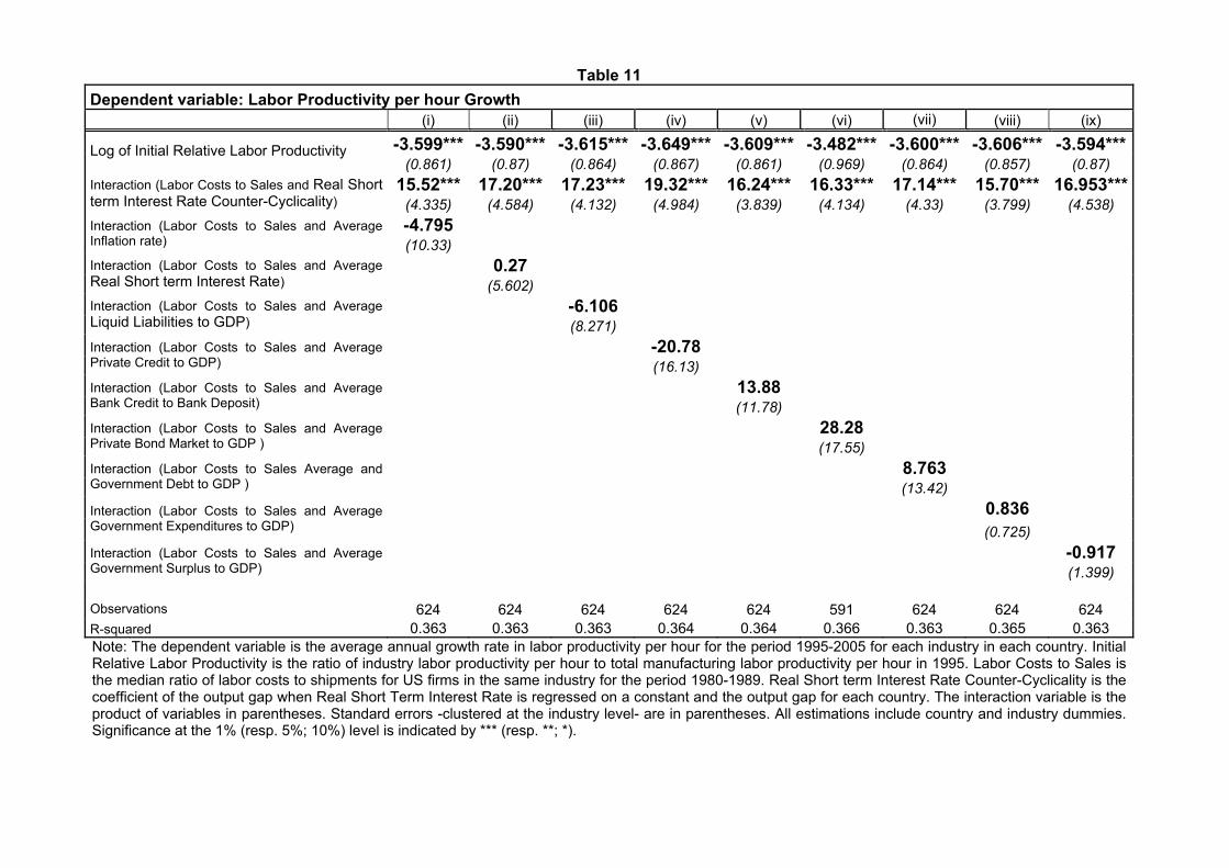
Table 11 Dependent variable: Labor Productivity per hour Growth
(i) (ii) (iii) (iv) (v) (vi) (vii) (viii) (ix)
-3.599*** -3.590*** -3.615*** -3.649*** -3.609*** -3.482*** -3.600*** -3.606*** -3.594*** Log of Initial Relative Labor Productivity (0.861) (0.87) (0.864) (0.867) (0.861) (0.969) (0.864) (0.857) (0.87)
15.52*** 17.20*** 17.23*** 19.32*** 16.24*** 16.33*** 17.14*** 15.70*** 16.953*** Interaction (Labor Costs to Sales and Real Short term Interest Rate Counter-Cyclicality) (4.335) (4.584) (4.132) (4.984) (3.839) (4.134) (4.33) (3.799) (4.538)
-4.795 Interaction (Labor Costs to Sales and Average Inflation rate) (10.33)
0.27 Interaction (Labor Costs to Sales and Average Real Short term Interest Rate) (5.602)
-6.106 Interaction (Labor Costs to Sales and Average Liquid Liabilities to GDP) (8.271)
-20.78 Interaction (Labor Costs to Sales and Average Private Credit to GDP) (16.13)
13.88 Interaction (Labor Costs to Sales and Average Bank Credit to Bank Deposit) (11.78)
28.28 Interaction (Labor Costs to Sales and Average Private Bond Market to GDP ) (17.55)
8.763 Interaction (Labor Costs to Sales Average and Government Debt to GDP ) (13.42)
0.836 Interaction (Labor Costs to Sales and Average Government Expenditures to GDP) (0.725)
-0.917 Interaction (Labor Costs to Sales and Average Government Surplus to GDP) (1.399) Observations 624 624 624 624 624 591 624 624 624 R-squared 0.363 0.363 0.363 0.364 0.364 0.366 0.363 0.365 0.363 Note: The dependent variable is the average annual growth rate in labor productivity per hour for the period 1995-2005 for each industry in each country. Initial Relative Labor Productivity is the ratio of industry labor productivity per hour to total manufacturing labor productivity per hour in 1995. Labor Costs to Sales is the median ratio of labor costs to shipments for US firms in the same industry for the period 1980-1989. Real Short term Interest Rate Counter-Cyclicality is the coefficient of the output gap when Real Short Term Interest Rate is regressed on a constant and the output gap for each country. The interaction variable is the product of variables in parentheses. Standard errors -clustered at the industry level- are in parentheses. All estimations include country and industry dummies. Significance at the 1% (resp. 5%; 10%) level is indicated by *** (resp. **; *).
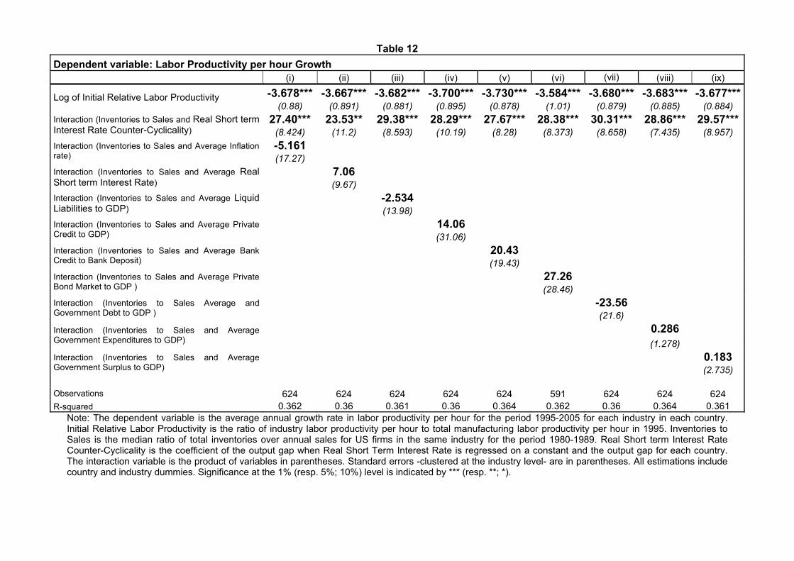
Table 12 Dependent variable: Labor Productivity per hour Growth
(i) (ii) (iii) (iv) (v) (vi) (vii) (viii) (ix)
-3.678*** -3.667*** -3.682*** -3.700*** -3.730*** -3.584*** -3.680*** -3.683*** -3.677*** Log of Initial Relative Labor Productivity (0.88) (0.891) (0.881) (0.895) (0.878) (1.01) (0.879) (0.885) (0.884)
27.40*** 23.53** 29.38*** 28.29*** 27.67*** 28.38*** 30.31*** 28.86*** 29.57*** Interaction (Inventories to Sales and Real Short term Interest Rate Counter-Cyclicality) (8.424) (11.2) (8.593) (10.19) (8.28) (8.373) (8.658) (7.435) (8.957)
-5.161 Interaction (Inventories to Sales and Average Inflation rate) (17.27)
7.06 Interaction (Inventories to Sales and Average Real Short term Interest Rate) (9.67)
-2.534 Interaction (Inventories to Sales and Average Liquid Liabilities to GDP) (13.98)
14.06 Interaction (Inventories to Sales and Average Private Credit to GDP) (31.06)
20.43 Interaction (Inventories to Sales and Average Bank Credit to Bank Deposit) (19.43)
27.26 Interaction (Inventories to Sales and Average Private Bond Market to GDP ) (28.46)
-23.56 Interaction (Inventories to Sales Average and Government Debt to GDP ) (21.6)
0.286 Interaction (Inventories to Sales and Average Government Expenditures to GDP) (1.278)
0.183 Interaction (Inventories to Sales and Average Government Surplus to GDP) (2.735) Observations 624 624 624 624 624 591 624 624 624 R-squared 0.362 0.36 0.361 0.36 0.364 0.362 0.36 0.364 0.361
Note: The dependent variable is the average annual growth rate in labor productivity per hour for the period 1995-2005 for each industry in each country. Initial Relative Labor Productivity is the ratio of industry labor productivity per hour to total manufacturing labor productivity per hour in 1995. Inventories to Sales is the median ratio of total inventories over annual sales for US firms in the same industry for the period 1980-1989. Real Short term Interest Rate Counter-Cyclicality is the coefficient of the output gap when Real Short Term Interest Rate is regressed on a constant and the output gap for each country. The interaction variable is the product of variables in parentheses. Standard errors -clustered at the industry level- are in parentheses. All estimations include country and industry dummies. Significance at the 1% (resp. 5%; 10%) level is indicated by *** (resp. **; *).
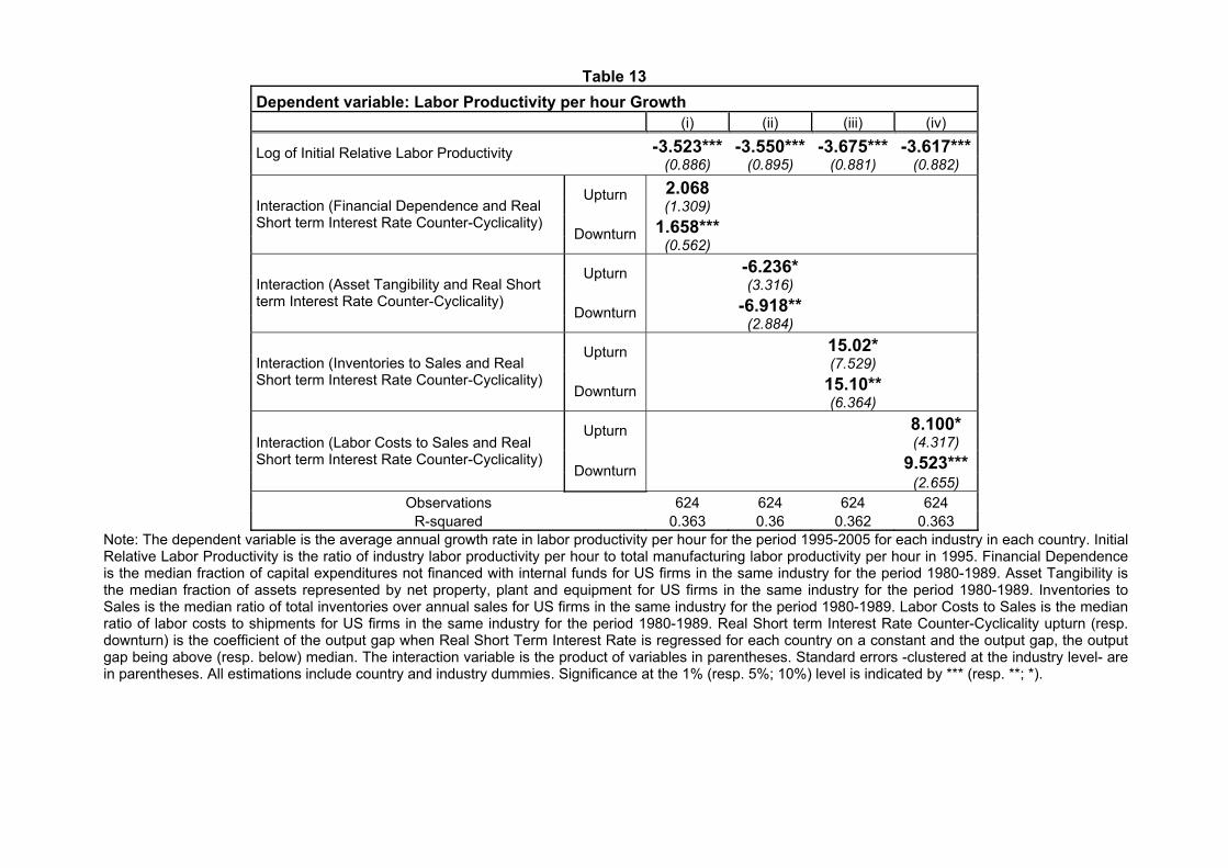
Table 13
Dependent variable: Labor Productivity per hour Growth (i) (ii) (iii) (iv)
-3.523*** -3.550*** -3.675*** -3.617***Log of Initial Relative Labor Productivity (0.886) (0.895) (0.881) (0.882) 2.068 Upturn (1.309)
1.658*** Interaction (Financial Dependence and Real Short term Interest Rate Counter-Cyclicality)
Downturn (0.562)
-6.236* Upturn (3.316) -6.918**
Interaction (Asset Tangibility and Real Short term Interest Rate Counter-Cyclicality)
Downturn (2.884) 15.02* Upturn (7.529) 15.10**
Interaction (Inventories to Sales and Real Short term Interest Rate Counter-Cyclicality)
Downturn (6.364) 8.100* Upturn (4.317) 9.523***
Interaction (Labor Costs to Sales and Real Short term Interest Rate Counter-Cyclicality)
Downturn (2.655)
Observations 624 624 624 624 R-squared 0.363 0.36 0.362 0.363
Note: The dependent variable is the average annual growth rate in labor productivity per hour for the period 1995-2005 for each industry in each country. Initial Relative Labor Productivity is the ratio of industry labor productivity per hour to total manufacturing labor productivity per hour in 1995. Financial Dependence is the median fraction of capital expenditures not financed with internal funds for US firms in the same industry for the period 1980-1989. Asset Tangibility is the median fraction of assets represented by net property, plant and equipment for US firms in the same industry for the period 1980-1989. Inventories to Sales is the median ratio of total inventories over annual sales for US firms in the same industry for the period 1980-1989. Labor Costs to Sales is the median ratio of labor costs to shipments for US firms in the same industry for the period 1980-1989. Real Short term Interest Rate Counter-Cyclicality upturn (resp. downturn) is the coefficient of the output gap when Real Short Term Interest Rate is regressed for each country on a constant and the output gap, the output gap being above (resp. below) median. The interaction variable is the product of variables in parentheses. Standard errors -clustered at the industry level- are in parentheses. All estimations include country and industry dummies. Significance at the 1% (resp. 5%; 10%) level is indicated by *** (resp. **; *).
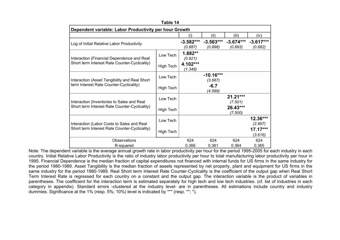
Table 14
Dependent variable: Labor Productivity per hour Growth (i) (ii) (iii) (iv)
-3.582*** -3.563*** -3.674*** -3.617***Log of Initial Relative Labor Productivity (0.887) (0.896) (0.893) (0.882)
1.882** Low Tech (0.821)
4.102*** Interaction (Financial Dependence and Real Short term Interest Rate Counter-Cyclicality)
High Tech(1.349)
-10.16*** Low Tech (3.687) -6.7
Interaction (Asset Tangibility and Real Short term Interest Rate Counter-Cyclicality)
High Tech (4.599) 21.21*** Low Tech (7.501) 26.43***
Interaction (Inventories to Sales and Real Short term Interest Rate Counter-Cyclicality)
High Tech (7.500) 12.36***Low Tech (2.897) 17.17***
Interaction (Labor Costs to Sales and Real Short term Interest Rate Counter-Cyclicality)
High Tech (3.616)
Observations 624 624 624 624 R-squared 0.366 0.361 0.364 0.365
Note: The dependent variable is the average annual growth rate in labor productivity per hour for the period 1995-2005 for each industry in each country. Initial Relative Labor Productivity is the ratio of industry labor productivity per hour to total manufacturing labor productivity per hour in 1995. Financial Dependence is the median fraction of capital expenditures not financed with internal funds for US firms in the same industry for the period 1980-1989. Asset Tangibility is the median fraction of assets represented by net property, plant and equipment for US firms in the same industry for the period 1980-1989. Real Short term Interest Rate Counter-Cyclicality is the coefficient of the output gap when Real Short Term Interest Rate is regressed for each country on a constant and the output gap. The interaction variable is the product of variables in parentheses. The coefficient for the interaction term is estimated separately for high tech and low tech industries. (cf. list of industries in each category in appendix). Standard errors -clustered at the industry level- are in parentheses. All estimations include country and industry dummies. Significance at the 1% (resp. 5%; 10%) level is indicated by *** (resp. **; *).
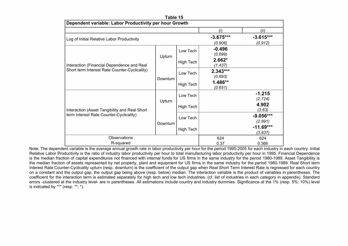
Table 15 Dependent variable: Labor Productivity per hour Growth (i) (ii)
-3.675*** -3.615*** Log of Initial Relative Labor Productivity (0.906) (0.912) -0.496 Low Tech (0.699) 2.662*
Upturn High Tech
(1.437) 2.343*** Low Tech
(0.693) 1.486**
Interaction (Financial Dependence and Real Short term Interest Rate Counter-Cyclicality)
DownturnHigh Tech
(0.651) -1.215 Low Tech (2.724) 4.902
Upturn High Tech
(3.63) -9.056*** Low Tech (2.991) -11.69***
Interaction (Asset Tangibility and Real Short term Interest Rate Counter-Cyclicality)
DownturnHigh Tech
(3.937) Observations 624 624
R-squared 0.37 0.366 Note: The dependent variable is the average annual growth rate in labor productivity per hour for the period 1995-2005 for each industry in each country. Initial Relative Labor Productivity is the ratio of industry labor productivity per hour to total manufacturing labor productivity per hour in 1995. Financial Dependence is the median fraction of capital expenditures not financed with internal funds for US firms in the same industry for the period 1980-1989. Asset Tangibility is the median fraction of assets represented by net property, plant and equipment for US firms in the same industry for the period 1980-1989. Real Short term Interest Rate Counter-Cyclicality upturn (resp. downturn) is the coefficient of the output gap when Real Short Term Interest Rate is regressed for each country on a constant and the output gap, the output gap being above (resp. below) median. The interaction variable is the product of variables in parentheses. The coefficient for the interaction term is estimated separately for high tech and low tech industries. (cf. list of industries in each category in appendix). Standard errors -clustered at the industry level- are in parentheses. All estimations include country and industry dummies. Significance at the 1% (resp. 5%; 10%) level is indicated by *** (resp. **; *).
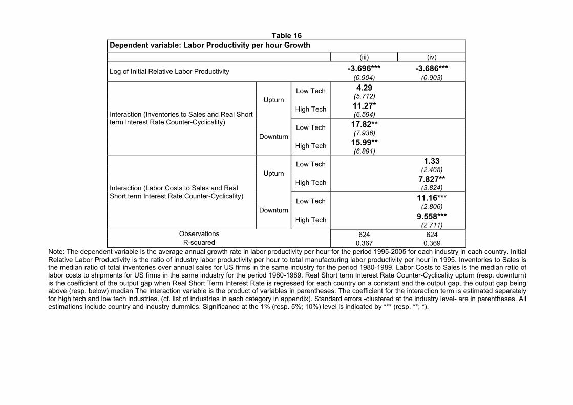
Table 16
Dependent variable: Labor Productivity per hour Growth (iii) (iv)
-3.696*** -3.686*** Log of Initial Relative Labor Productivity (0.904) (0.903) 4.29 Low Tech
(5.712) 11.27*
Upturn High Tech
(6.594) 17.82** Low Tech (7.936)
15.99**
Interaction (Inventories to Sales and Real Short term Interest Rate Counter-Cyclicality)
DownturnHigh Tech
(6.891) 1.33 Low Tech (2.465) 7.827**
Upturn High Tech
(3.824) 11.16*** Low Tech (2.806) 9.558***
Interaction (Labor Costs to Sales and Real Short term Interest Rate Counter-Cyclicality)
DownturnHigh Tech
(2.711) Observations 624 624
R-squared 0.367 0.369 Note: The dependent variable is the average annual growth rate in labor productivity per hour for the period 1995-2005 for each industry in each country. Initial Relative Labor Productivity is the ratio of industry labor productivity per hour to total manufacturing labor productivity per hour in 1995. Inventories to Sales is the median ratio of total inventories over annual sales for US firms in the same industry for the period 1980-1989. Labor Costs to Sales is the median ratio of labor costs to shipments for US firms in the same industry for the period 1980-1989. Real Short term Interest Rate Counter-Cyclicality upturn (resp. downturn) is the coefficient of the output gap when Real Short Term Interest Rate is regressed for each country on a constant and the output gap, the output gap being above (resp. below) median The interaction variable is the product of variables in parentheses. The coefficient for the interaction term is estimated separately for high tech and low tech industries. (cf. list of industries in each category in appendix). Standard errors -clustered at the industry level- are in parentheses. All estimations include country and industry dummies. Significance at the 1% (resp. 5%; 10%) level is indicated by *** (resp. **; *).