Logistics Management

Customer Service

Özgür Kabak, Ph.D.

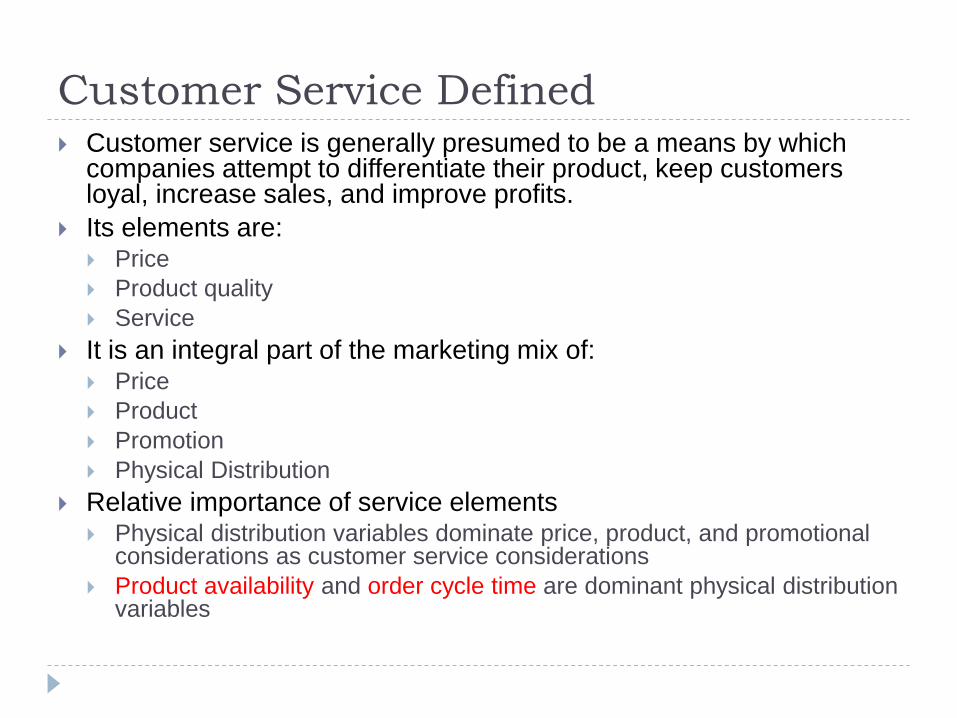
Customer Service Defined Customer service is generally presumed to be a means by which

companies attempt to differentiate their product, keep customers loyal, increase sales, and improve profits.

Its elements are: Price

Product quality

Service

It is an integral part of the marketing mix of: Price

Product

Promotion

Physical Distribution

Relative importance of service elements Physical distribution variables dominate price, product, and promotional

considerations as customer service considerations

Product availability and order cycle time are dominant physical distribution variables

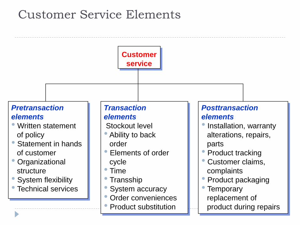
Customer Service Elements

Customer

service

Pretransaction

elements

• Written statement

of policy

• Statement in hands

of customer

• Organizational

structure

• System flexibility

• Technical services

Transaction

elements

Stockout level

• Ability to back

order

• Elements of order

cycle

• Time

• Transship

• System accuracy

• Order conveniences

• Product substitution

Posttransaction

elements

• Installation, warranty

alterations, repairs,

parts

• Product tracking

• Customer claims,

complaints

• Product packaging

• Temporary

replacement of

product during repairs

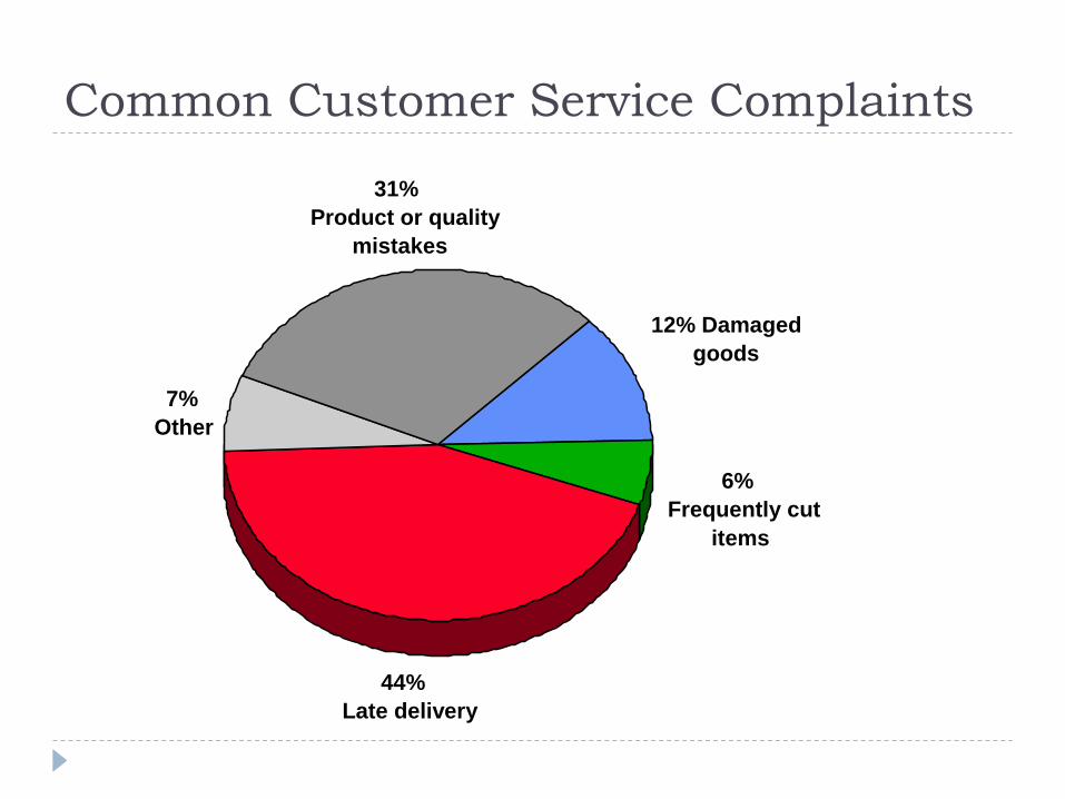
Common Customer Service Complaints

12% Damaged

goods

31%

Product or quality

mistakes

7%

Other

6%

Frequently cut

items

44%

Late delivery

Most Important Customer Service Elements

On-time delivery

Order fill rate

Product condition

Accurate documentation

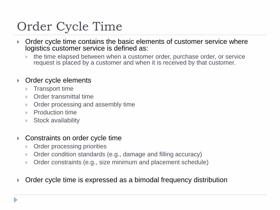
Order Cycle Time Order cycle time contains the basic elements of customer service where

logistics customer service is defined as: the time elapsed between when a customer order, purchase order, or service

request is placed by a customer and when it is received by that customer.

Order cycle elements Transport time

Order transmittal time

Order processing and assembly time

Production time

Stock availability

Constraints on order cycle time Order processing priorities

Order condition standards (e.g., damage and filling accuracy)

Order constraints (e.g., size minimum and placement schedule)

Order cycle time is expressed as a bimodal frequency distribution

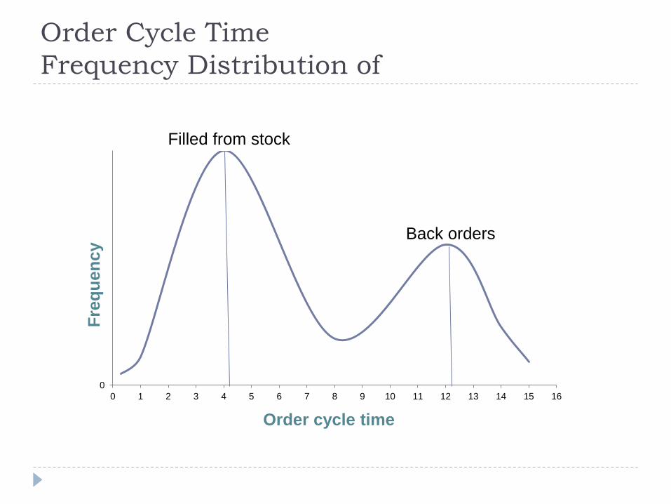
Order Cycle Time

Frequency Distribution of

0

0 1 2 3 4 5 6 7 8 9 10 11 12 13 14 15 16

Filled from stock

Back orders

Order cycle time

Fre

qu

en

cy

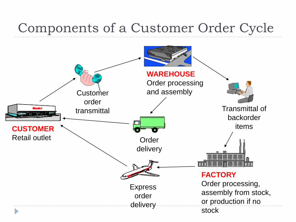
Components of a Customer Order Cycle

CUSTOMER

Retail outlet

Customer

order

transmittal Transmittal of

backorder

items

Order

delivery

Express

order

delivery

FACTORY

Order processing,

assembly from stock,

or production if no

stock

WAREHOUSE

Order processing

and assembly

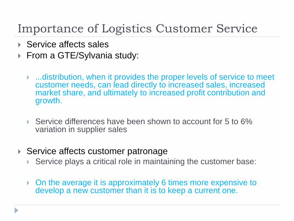
Importance of Logistics Customer Service

Service affects sales

From a GTE/Sylvania study:

...distribution, when it provides the proper levels of service to meet

customer needs, can lead directly to increased sales, increased market share, and ultimately to increased profit contribution and growth.

Service differences have been shown to account for 5 to 6%

variation in supplier sales

Service affects customer patronage Service plays a critical role in maintaining the customer base:

On the average it is approximately 6 times more expensive to

develop a new customer than it is to keep a current one.

Service Observations

The dominant customer service elements are

logistical in nature

Late delivery is the most common service complaint

and speed of delivery is the most important service

element

The penalty for service failure is primarily reduced

patronage, i.e., lost sales

The logistics customer service effect on sales is

difficult to determine

Service Level Optimization

Optimal inventory policy assumes a specific service level target.

What is the appropriate level of service? May be determined by the downstream customer

Retailer may require the supplier, to maintain a specific service level

Supplier will use that target to manage its own inventory

Facility may have the flexibility to choose the appropriate level of service

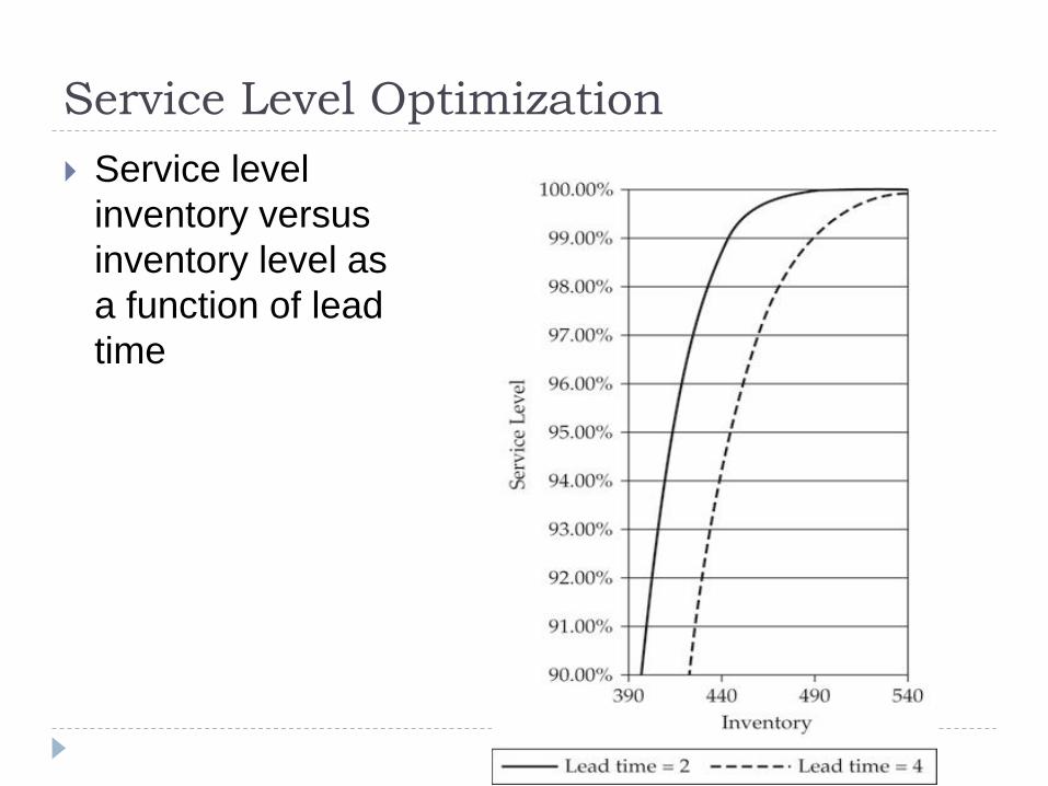
Service Level Optimization

Service level

inventory versus

inventory level as

a function of lead

time

Trade-Offs

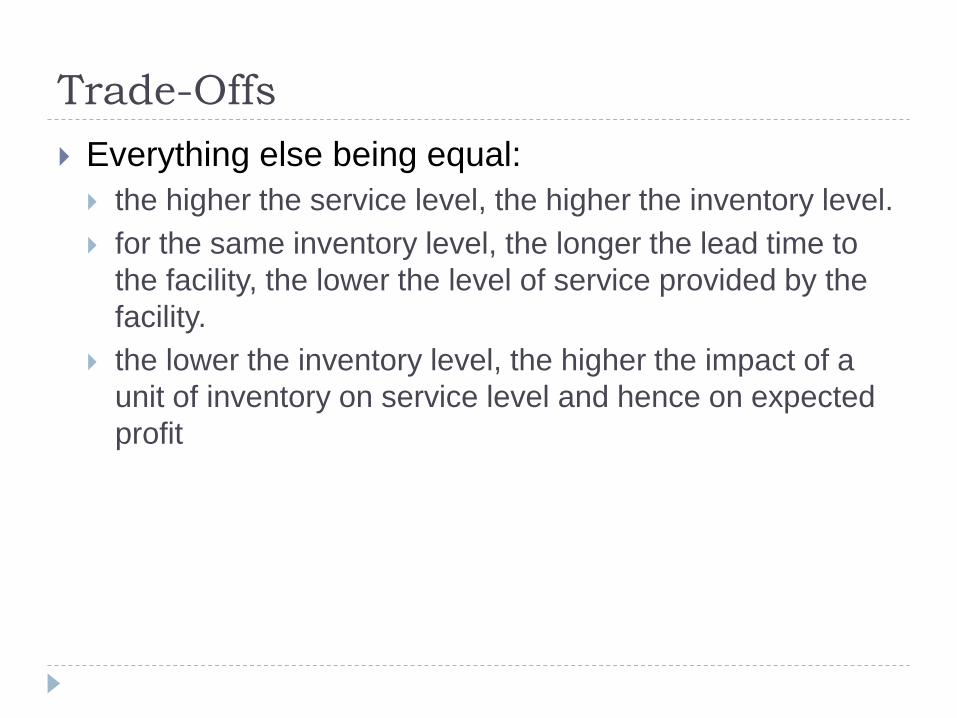
Everything else being equal:

the higher the service level, the higher the inventory level.

for the same inventory level, the longer the lead time to

the facility, the lower the level of service provided by the

facility.

the lower the inventory level, the higher the impact of a

unit of inventory on service level and hence on expected

profit

Steps to Follows in Determining the

Service Standards

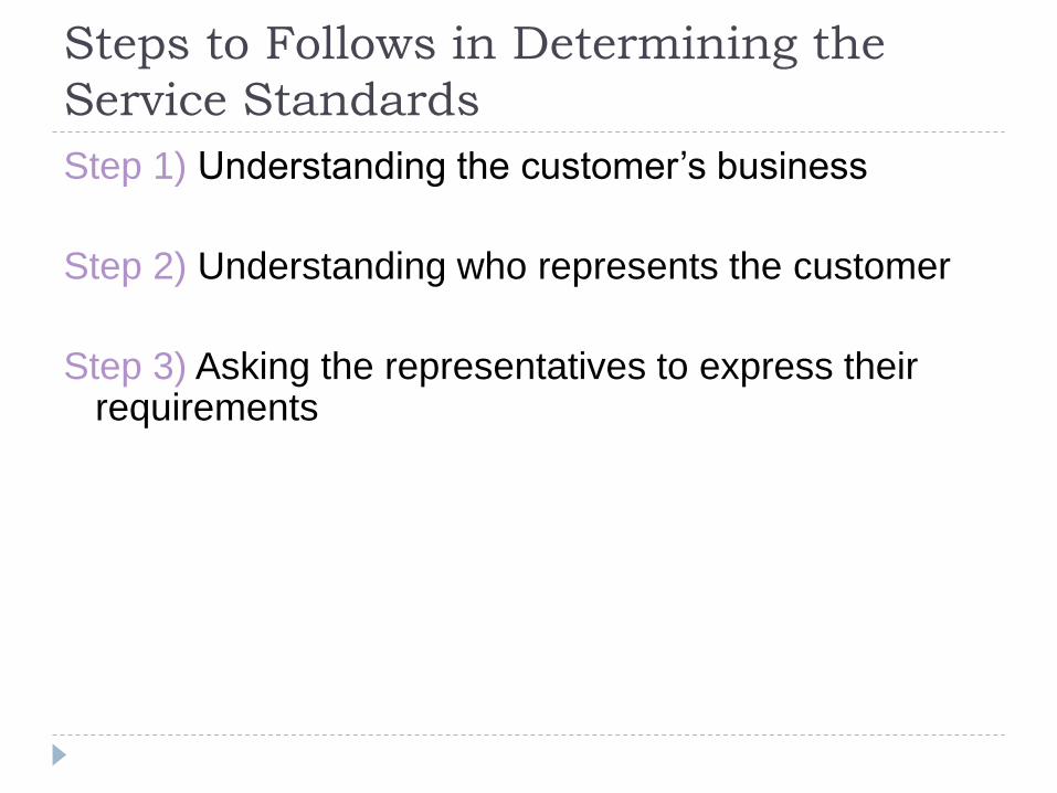
Step 1) Understanding the customer’s business

Step 2) Understanding who represents the customer

Step 3) Asking the representatives to express their requirements

Methods of Identifying Requirements

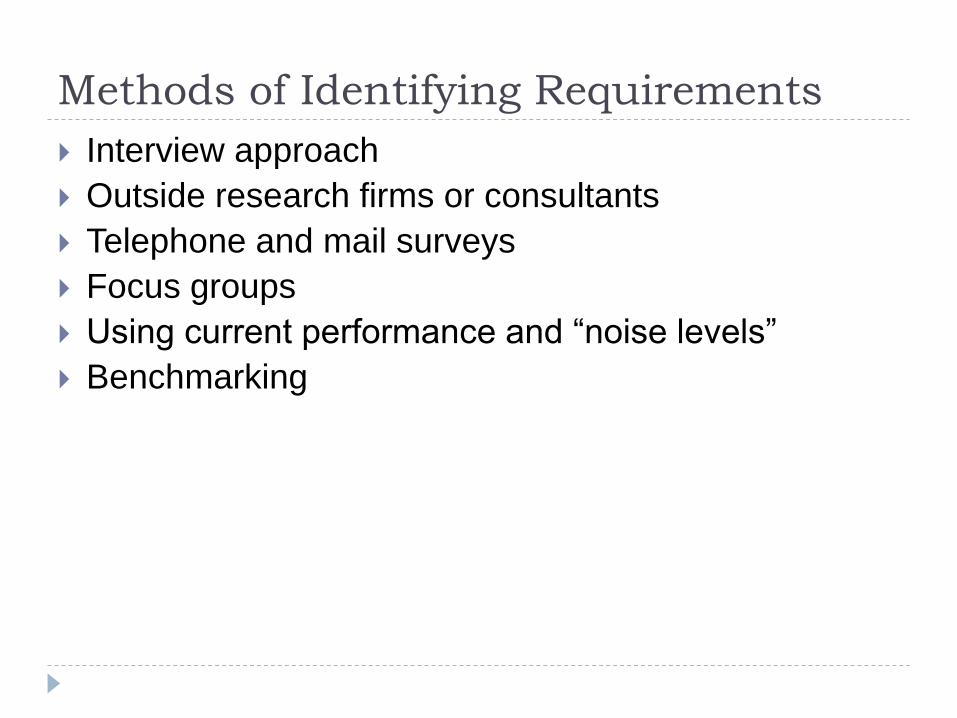
Interview approach

Outside research firms or consultants

Telephone and mail surveys

Focus groups

Using current performance and “noise levels”

Benchmarking

Understanding Requirements of the Order

Fulfillment Process

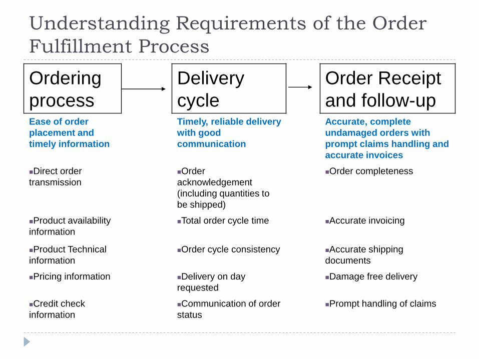
Ordering

process

Delivery

cycle

Order Receipt

and follow-up Ease of order

placement and

timely information

Timely, reliable delivery

with good

communication

Accurate, complete

undamaged orders with

prompt claims handling and

accurate invoices

Direct order

transmission

Order

acknowledgement

(including quantities to

be shipped)

Order completeness

Product availability

information

Total order cycle time

Accurate invoicing

Product Technical

information

Order cycle consistency

Accurate shipping

documents

Pricing information Delivery on day

requested

Damage free delivery

Credit check

information

Communication of order

status

Prompt handling of claims

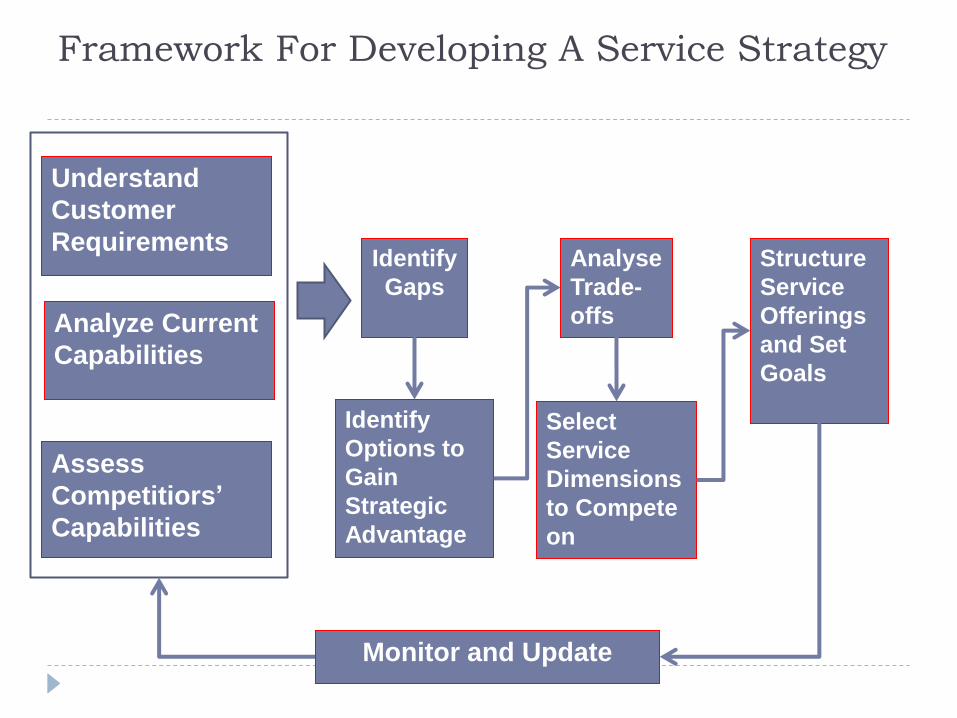
Framework For Developing A Service Strategy

Understand

Customer

Requirements

Analyze Current

Capabilities

Assess

Competitiors’

Capabilities

Identify

Gaps

Identify

Options to

Gain

Strategic

Advantage

Analyse

Trade-

offs

Select

Service

Dimensions

to Compete

on

Structure

Service

Offerings

and Set

Goals

Monitor and Update

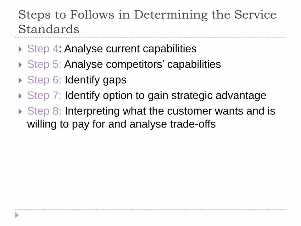
Steps to Follows in Determining the Service

Standards

Step 4: Analyse current capabilities

Step 5: Analyse competitors’ capabilities

Step 6: Identify gaps

Step 7: Identify option to gain strategic advantage

Step 8: Interpreting what the customer wants and is

willing to pay for and analyse trade-offs

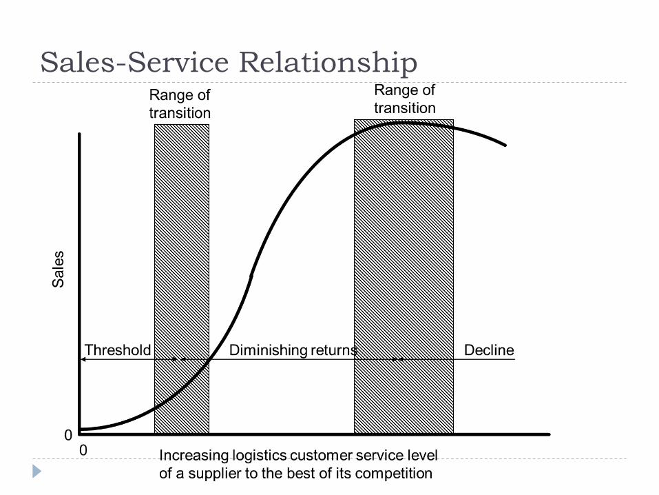
Sales-Service Relationship

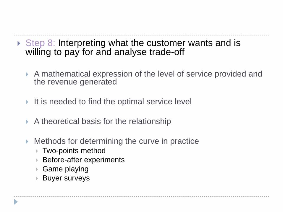
Step 8: Interpreting what the customer wants and is willing to pay for and analyse trade-off

A mathematical expression of the level of service provided and

the revenue generated

It is needed to find the optimal service level

A theoretical basis for the relationship

Methods for determining the curve in practice Two-points method

Before-after experiments

Game playing

Buyer surveys

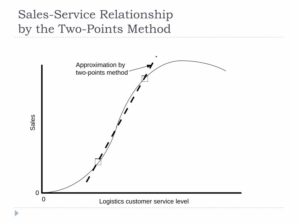
Sales-Service Relationship

by the Two-Points Method

Logistics customer service level

Sale

s

00

Approximation by

two-points method

Determining Optimum Service Levels

Cost vs. Service

Theory

Optimum profit is the point where profit contribution

equals marginal cost

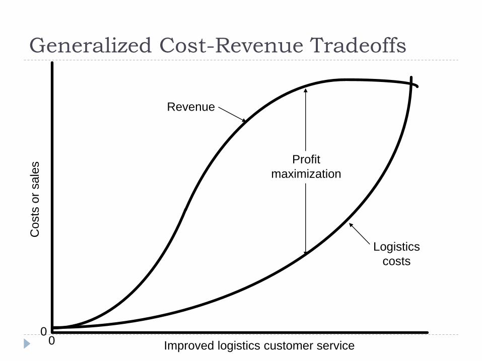
Generalized Cost-Revenue Tradeoffs

Profit

maximization

Revenue

Logistics

costs

Improved logistics customer service 0 0

Costs

or

sale

s

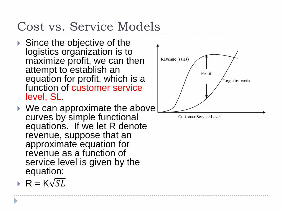
Cost vs. Service Models

Since the objective of the logistics organization is to maximize profit, we can then attempt to establish an equation for profit, which is a function of customer service level, SL.

We can approximate the above curves by simple functional equations. If we let R denote revenue, suppose that an approximate equation for revenue as a function of service level is given by the equation:

R = K 𝑆𝐿

Cost vs. Service Models

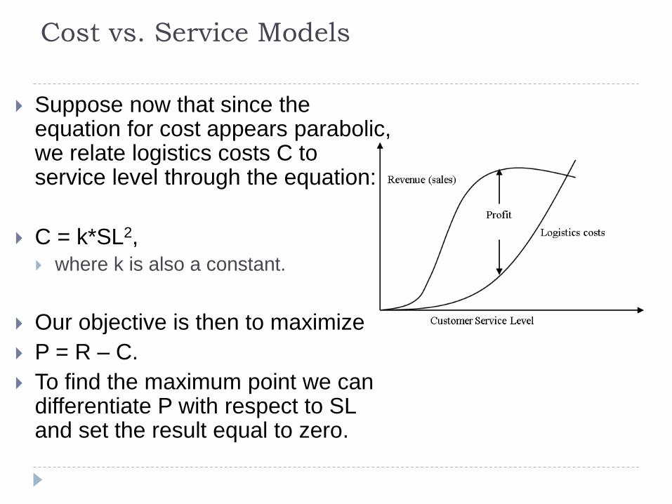
Suppose now that since the equation for cost appears parabolic, we relate logistics costs C to service level through the equation:

C = k*SL2,

where k is also a constant.

Our objective is then to maximize

P = R – C.

To find the maximum point we can differentiate P with respect to SL and set the result equal to zero.

EXAMPLE

SL Revenue (1000TL)

Logistics

Cost (1000 TL)

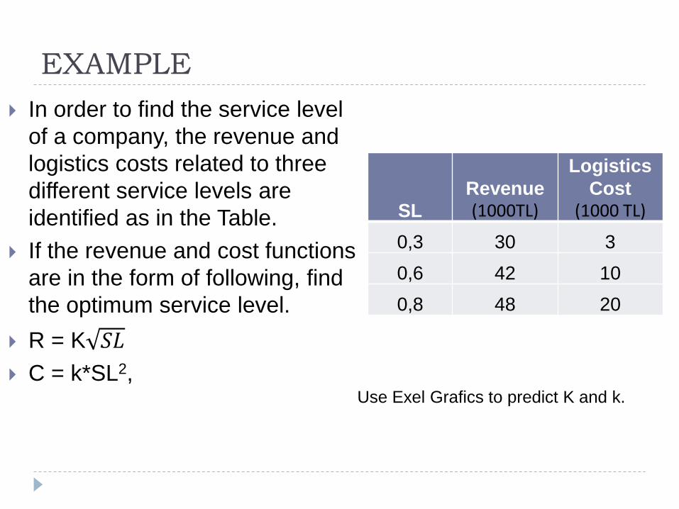
0,3 30 3

0,6 42 10

0,8 48 20

In order to find the service level

of a company, the revenue and

logistics costs related to three

different service levels are

identified as in the Table.

If the revenue and cost functions

are in the form of following, find

the optimum service level.

R = K 𝑆𝐿

C = k*SL2,

Use Exel Grafics to predict K and k.

Cost vs. Service Models

Polynomial Equations

A polynomial is an equation that has only two

variables (X and Y), but may have many terms on

the right-hand-side.

Y = a0 + a1X + a2X2+…+anX

n

When the highest power of X is n, the polynomial is said to be of order n..

A polynomial of order 2 is xcalled quadratic equation Y=a0 + a1X + a2 X

2

Cost vs. Service Models

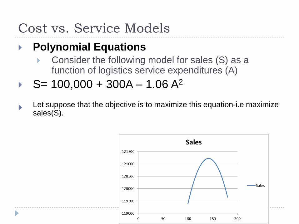
Polynomial Equations Consider the following model for sales (S) as a

function of logistics service expenditures (A)

S= 100,000 + 300A – 1.06 A2

Let suppose that the objective is to maximize this equation-i.e maximize sales(S).

Cost vs. Service Models

Power Equations

Power equations have one term on the right-hand

side-a variable raised to some power.

General power equation: Y=aX b

The learning curve is an interesting application of power equations. This

application stems from the many business situations where it takes time to

learn to perform a task-.the onger the task is performed, the better the

performance.Output=a(Input)b

Cost vs. Service Models

Practice

For a constant rate,

R = trading margin sales response rate annual

sales

C = annual carrying cost standard product cost

demand standard deviation over replenishment lead-

time z

Set R = C and find z corresponding to a specific

service level

Cost vs. Service Models

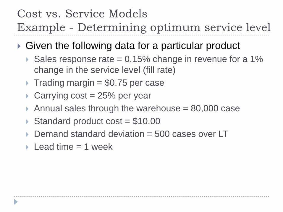
Example - Determining optimum service level

Given the following data for a particular product

Sales response rate = 0.15% change in revenue for a 1%

change in the service level (fill rate)

Trading margin = $0.75 per case

Carrying cost = 25% per year

Annual sales through the warehouse = 80,000 case

Standard product cost = $10.00

Demand standard deviation = 500 cases over LT

Lead time = 1 week

Cost vs. Service Models

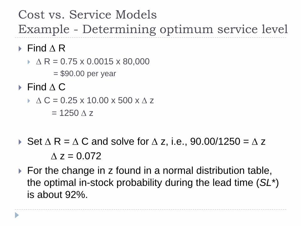
Example - Determining optimum service level

Find R

R = 0.75 x 0.0015 x 80,000

= $90.00 per year

Find C

C = 0.25 x 10.00 x 500 x z

= 1250 z

Set R = C and solve for z, i.e., 90.00/1250 = z

z = 0.072

For the change in z found in a normal distribution table,

the optimal in-stock probability during the lead time (SL*)

is about 92%.

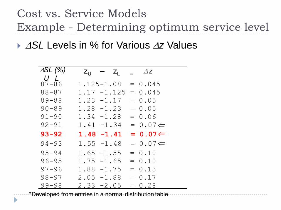
Cost vs. Service Models

Example - Determining optimum service level

SL Levels in % for Various z Values

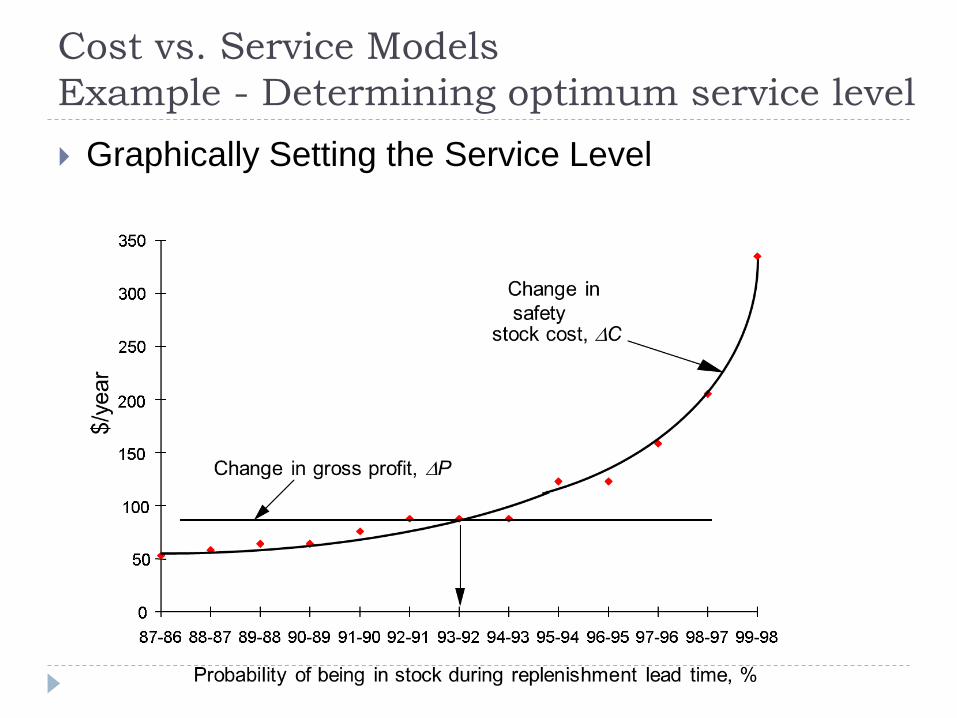
Cost vs. Service Models

Example - Determining optimum service level

Graphically Setting the Service Level

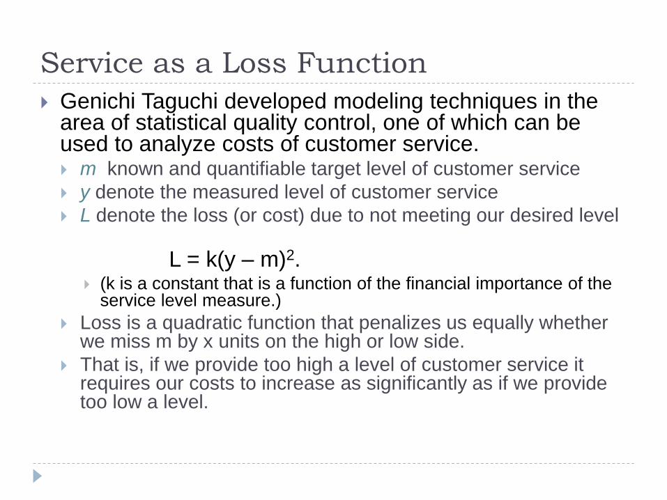
Service as a Loss Function

Genichi Taguchi developed modeling techniques in the area of statistical quality control, one of which can be used to analyze costs of customer service. m known and quantifiable target level of customer service

y denote the measured level of customer service

L denote the loss (or cost) due to not meeting our desired level

L = k(y – m)2. (k is a constant that is a function of the financial importance of the

service level measure.)

Loss is a quadratic function that penalizes us equally whether we miss m by x units on the high or low side.

That is, if we provide too high a level of customer service it requires our costs to increase as significantly as if we provide too low a level.

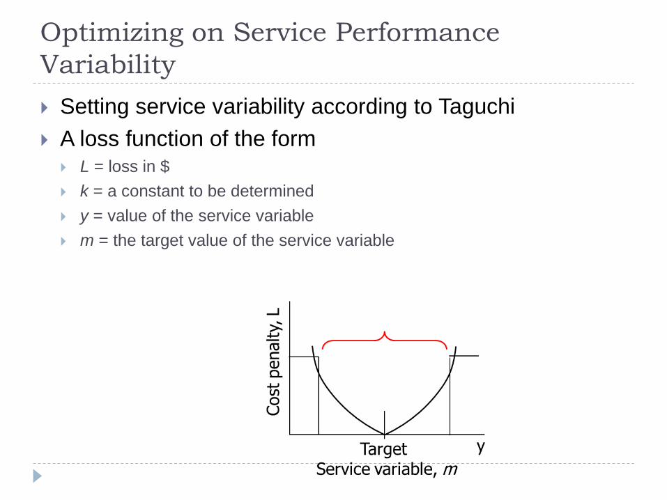
Optimizing on Service Performance

Variability

Setting service variability according to Taguchi

A loss function of the form L = loss in $

k = a constant to be determined

y = value of the service variable

m = the target value of the service variable

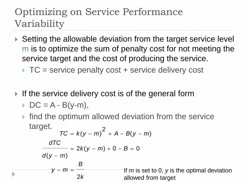
Optimizing on Service Performance

Variability

Setting the allowable deviation from the target service level

m is to optimize the sum of penalty cost for not meeting the

service target and the cost of producing the service.

TC = service penalty cost + service delivery cost

If the service delivery cost is of the general form

DC = A - B(y-m),

find the optimum allowed deviation from the service

target.

k

Bmy

Bmykmyd

dTC

myBAmykTC

2

00)(2)(

)(2

)(

If m is set to 0, y is the optimal deviation

allowed from target

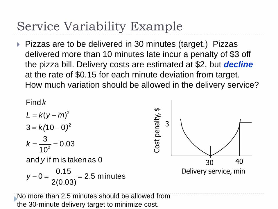
Service Variability Example

Pizzas are to be delivered in 30 minutes (target.) Pizzas

delivered more than 10 minutes late incur a penalty of $3 off

the pizza bill. Delivery costs are estimated at $2, but decline

at the rate of $0.15 for each minute deviation from target.

How much variation should be allowed in the delivery service?

minutes2.52(0.03)

0.150

0as taken is m ifand

0.0310

3

0103

)(

Find

2

2

y

y

k

)k(

mykL

k

2

No more than 2.5 minutes should be allowed from

the 30-minute delivery target to minimize cost.

Service as a Constraint

Practitioners often find these constants, such as k and K, difficult to

quantify, since we don’t know exactly how customers will react to

poor service. For this reason we often find constraints on service

levels implemented in practice, e.g., the firm targets a level of no

more than 2% stockouts per period or specifies 99% of orders are

received within 1 week of order placement. This gives alternatives

when creating an optimization model with respect to system costs or

profits:

Either we create a term in our objective function that captures cost

as a function of service level, or

We create constraints that require our decision variables to satisfy

a certain minimum level of service.

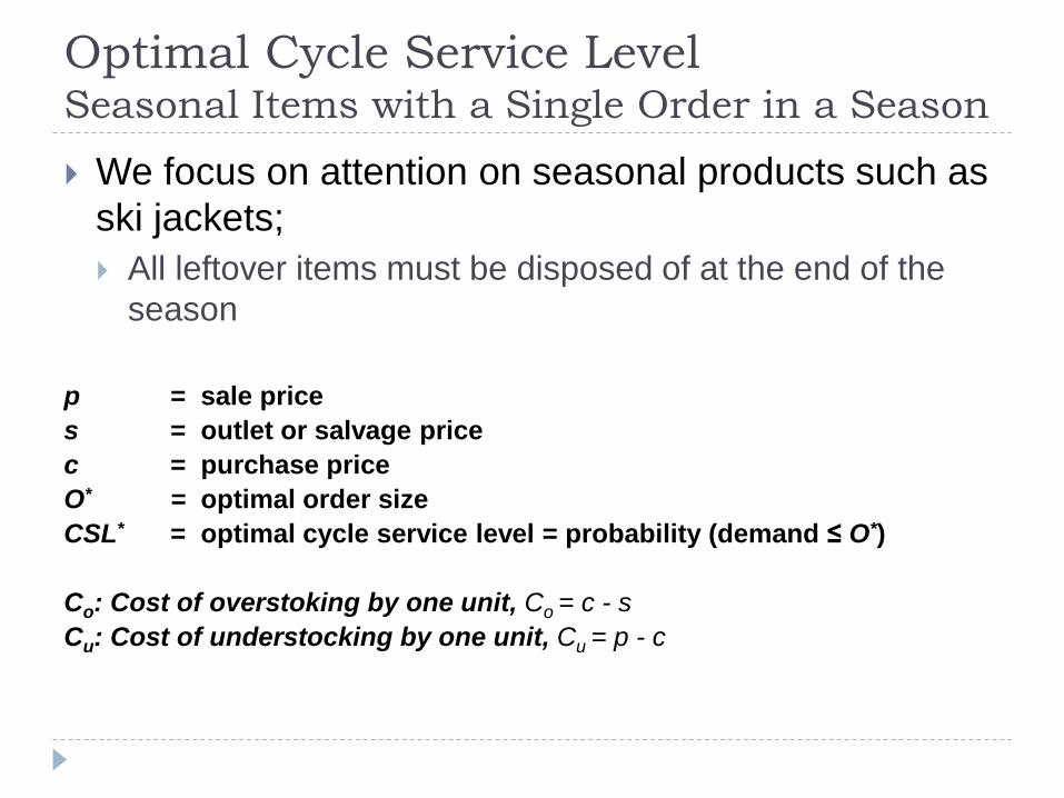
Optimal Cycle Service Level Seasonal Items with a Single Order in a Season

We focus on attention on seasonal products such as

ski jackets;

All leftover items must be disposed of at the end of the

season

p = sale price

s = outlet or salvage price

c = purchase price

O* = optimal order size

CSL* = optimal cycle service level = probability (demand ≤ O*)

Co: Cost of overstoking by one unit, Co = c - s

Cu: Cost of understocking by one unit, Cu = p - c

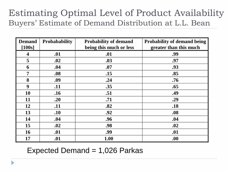
Estimating Optimal Level of Product Availability Buyers’ Estimate of Demand Distribution at L.L. Bean

Demand

[100s]

Probabability Probability of demand

being this much or less

Probability of demand being

greater than this much

4 .01 .01 .99

5 .02 .03 .97

6 .04 .07 .93

7 .08 .15 .85

8 .09 .24 .76

9 .11 .35 .65

10 .16 .51 .49

11 .20 .71 .29

12 .11 .82 .18

13 .10 .92 .08

14 .04 .96 .04

15 .02 .98 .02

16 .01 .99 .01

17 .01 1.00 .00

Expected Demand = 1,026 Parkas

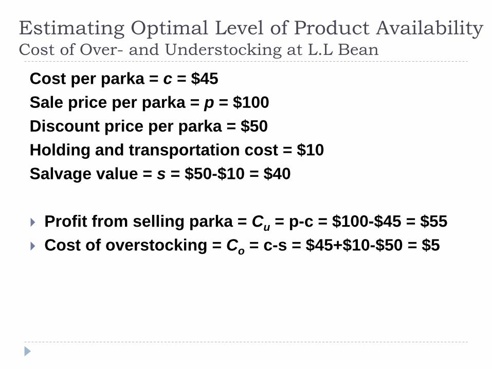
Estimating Optimal Level of Product Availability Cost of Over- and Understocking at L.L Bean

Cost per parka = c = $45

Sale price per parka = p = $100

Discount price per parka = $50

Holding and transportation cost = $10

Salvage value = s = $50-$10 = $40

Profit from selling parka = Cu = p-c = $100-$45 = $55

Cost of overstocking = Co = c-s = $45+$10-$50 = $5

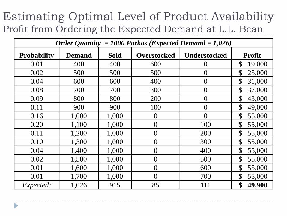
Estimating Optimal Level of Product Availability Profit from Ordering the Expected Demand at L.L. Bean

Order Quantity = 1000 Parkas (Expected Demand = 1,026)

Probability Demand Sold Overstocked Understocked Profit

0.01 400 400 600 0 $ 19,000

0.02 500 500 500 0 $ 25,000

0.04 600 600 400 0 $ 31,000

0.08 700 700 300 0 $ 37,000

0.09 800 800 200 0 $ 43,000

0.11 900 900 100 0 $ 49,000

0.16 1,000 1,000 0 0 $ 55,000

0.20 1,100 1,000 0 100 $ 55,000

0.11 1,200 1,000 0 200 $ 55,000

0.10 1,300 1,000 0 300 $ 55,000

0.04 1,400 1,000 0 400 $ 55,000

0.02 1,500 1,000 0 500 $ 55,000

0.01 1,600 1,000 0 600 $ 55,000

0.01 1,700 1,000 0 700 $ 55,000

Expected: 1,026 915 85 111 $ 49,900

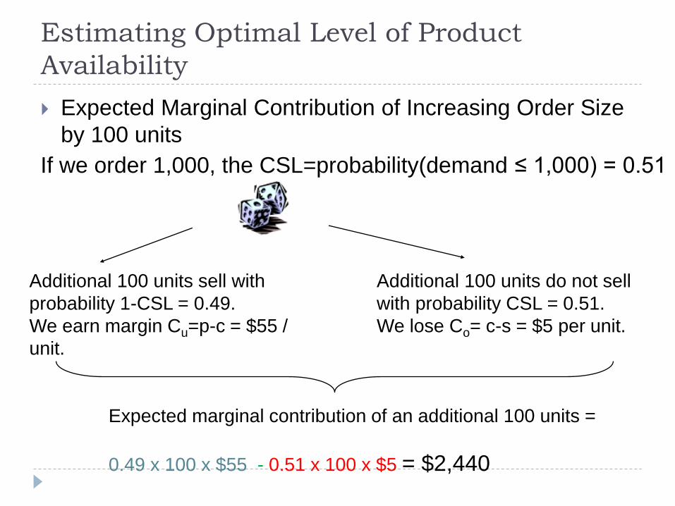
Estimating Optimal Level of Product

Availability

Expected Marginal Contribution of Increasing Order Size

by 100 units

If we order 1,000, the CSL=probability(demand ≤ 1,000) = 0.51

Expected marginal contribution of an additional 100 units =

0.49 x 100 x $55 - 0.51 x 100 x $5 = $2,440

Additional 100 units sell with

probability 1-CSL = 0.49.

We earn margin Cu=p-c = $55 /

unit.

Additional 100 units do not sell

with probability CSL = 0.51.

We lose Co= c-s = $5 per unit.

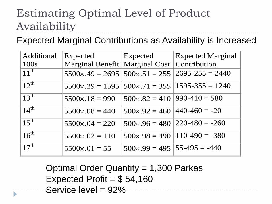
Estimating Optimal Level of Product

Availability

Additional

100s

Expected

Marginal Benefit

Expected

Marginal Cost

Expected Marginal

Contribution

11th5500.49 = 2695 500.51 = 255 2695-255 = 2440

12th5500.29 = 1595 500.71 = 355 1595-355 = 1240

13th5500.18 = 990 500.82 = 410 990-410 = 580

14th5500.08 = 440 500.92 = 460 440-460 = -20

15th5500.04 = 220 500.96 = 480 220-480 = -260

16th

5500.02 = 110 500.98 = 490 110-490 = -380

17th5500.01 = 55 500.99 = 495 55-495 = -440

Optimal Order Quantity = 1,300 Parkas

Expected Profit = $ 54,160

Service level = 92%

Expected Marginal Contributions as Availability is Increased

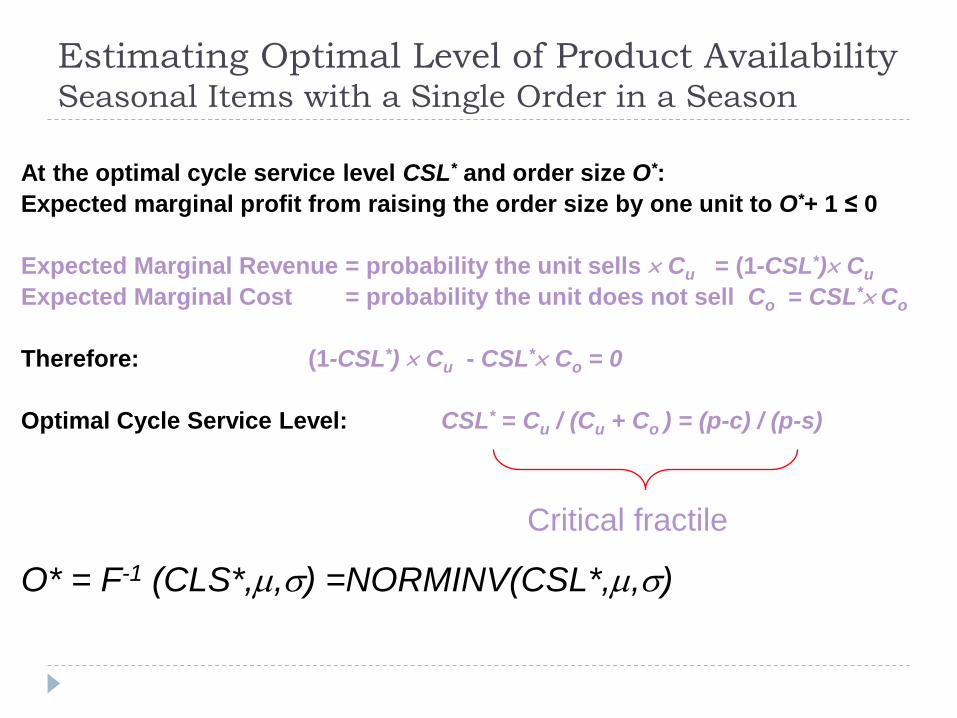
Estimating Optimal Level of Product Availability Seasonal Items with a Single Order in a Season

At the optimal cycle service level CSL* and order size O*:

Expected marginal profit from raising the order size by one unit to O*+ 1 ≤ 0

Expected Marginal Revenue = probability the unit sells Cu = (1-CSL*) Cu

Expected Marginal Cost = probability the unit does not sell Co = CSL* Co

Therefore: (1-CSL*) Cu - CSL* Co = 0

Optimal Cycle Service Level: CSL* = Cu / (Cu + Co ) = (p-c) / (p-s)

O* = F-1 (CLS*,,) =NORMINV(CSL*,,)

Critical fractile

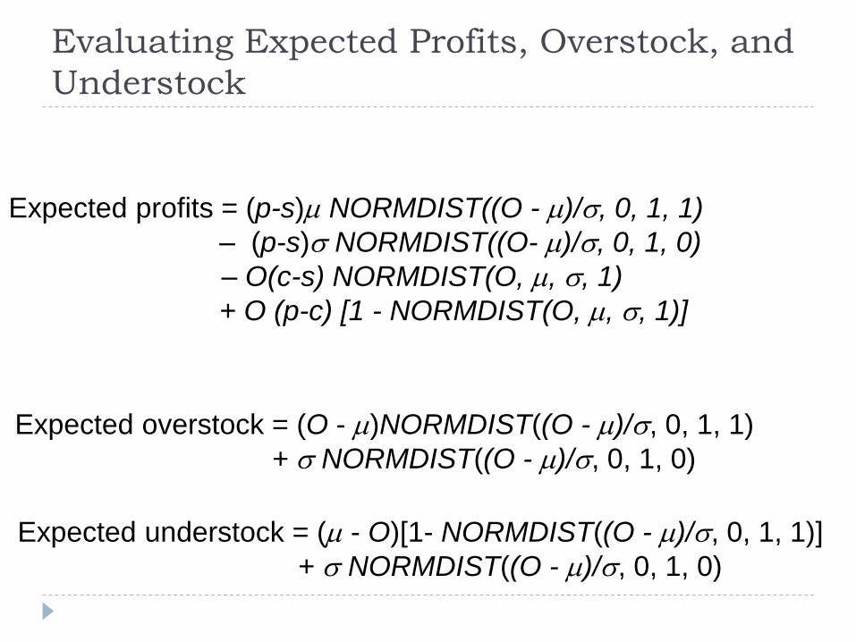
Evaluating Expected Profits, Overstock, and

Understock

Expected profits = (p-s) NORMDIST((O - )/, 0, 1, 1)

– (p-s) NORMDIST((O- )/, 0, 1, 0)

– O(c-s) NORMDIST(O, , , 1)

+ O (p-c) [1 - NORMDIST(O, , , 1)]

Expected overstock = (O - )NORMDIST((O - )/, 0, 1, 1)

+ NORMDIST((O - )/, 0, 1, 0)

Expected understock = ( - O)[1- NORMDIST((O - )/, 0, 1, 1)]

+ NORMDIST((O - )/, 0, 1, 0)

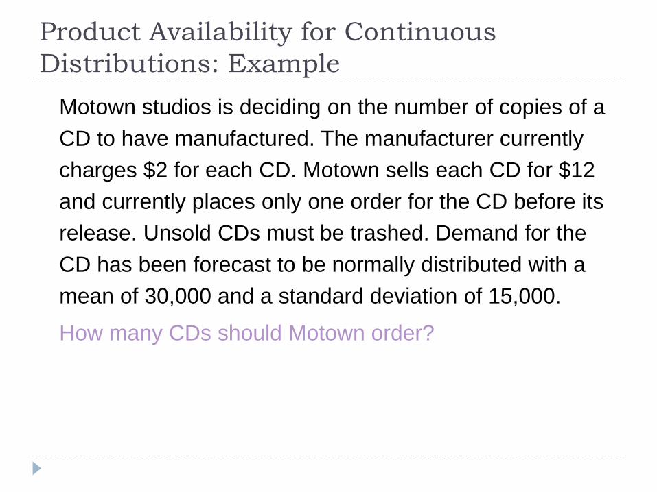
Product Availability for Continuous

Distributions: Example

Motown studios is deciding on the number of copies of a

CD to have manufactured. The manufacturer currently

charges $2 for each CD. Motown sells each CD for $12

and currently places only one order for the CD before its

release. Unsold CDs must be trashed. Demand for the

CD has been forecast to be normally distributed with a

mean of 30,000 and a standard deviation of 15,000.

How many CDs should Motown order?