Jim Stock and Mark Watson - Becker Friedman Institute · 1 Disentangling the Channels of the...
55
1 Disentangling the Channels of the 2007-09 Recession Jim Stock and Mark Watson
-
Upload
truongdien -
Category
Documents
-
view
215 -
download
0
Transcript of Jim Stock and Mark Watson - Becker Friedman Institute · 1 Disentangling the Channels of the...

1
Disentangling the Channels of the 2007-09 Recession
Jim Stock and Mark Watson
2
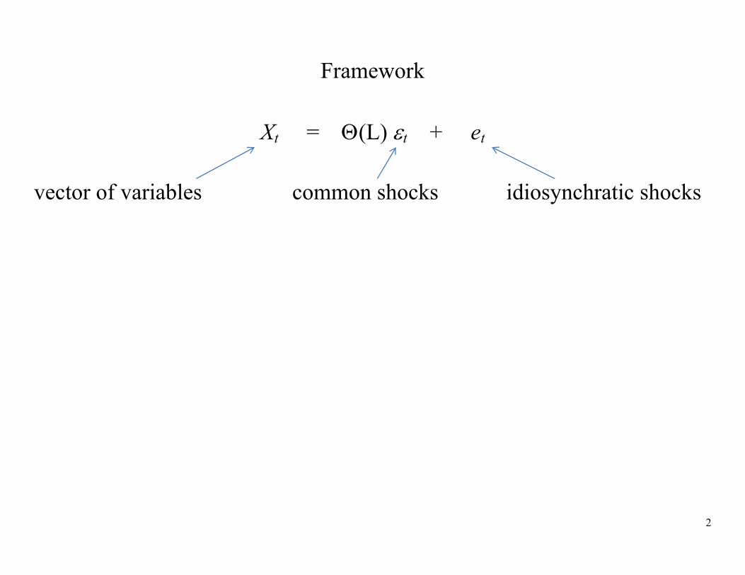
Framework
Xt = (L) t + et
vector of variables common shocks idiosynchratic shocks
3
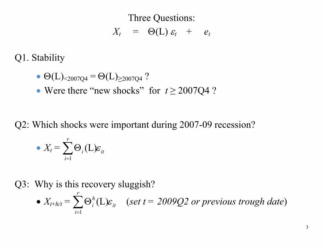
Three Questions: Xt = (L) t + et
Q1. Stability
(L)<2007Q4 = (L)≥2007Q4 ? Were there “new shocks” for t ≥ 2007Q4 ?
Q2: Which shocks were important during 2007-09 recession?
Xt = 1
(L)r
i iti
Q3: Why is this recovery sluggish?
Xt+h/t = 1
(L)r
hi it
i
(set t = 2009Q2 or previous trough date)
4
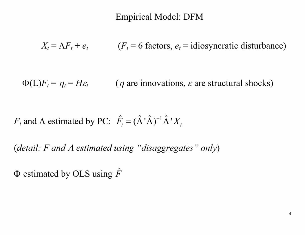
Empirical Model: DFM
Xt = Ft + et (Ft = 6 factors, et = idiosyncratic disturbance)
(L)Ft = t = Ht ( are innovations, are structural shocks) Ft and estimated by PC: 1ˆ ˆ ˆ ˆ( ' ) 't tF X (detail: F and estimated using “disaggregates” only) estimated by OLS using F

5
Xt = Ft + et (L)Ft = t Q1: Stability, new shocks, etc.
from t < 2007Q4 data and 1ˆ ˆ ˆ ˆ( ' ) 't tF X for all t
ˆ ˆ ˆt t tX F e
How does “fit” over t ≥ 2007Q4 compare to t < 2007Q4?
Does te for t ≥ 2007Q4 contain a common shock?
Are and stable across t = 2007Q4?

6
Xt = Ft + et (L)Ft = t = Ht
Q2: Which shocks were important during 2007-09?
Innovation in Xjt = j’t = j’Ht
SVAR analysis: t = H−1t
o “External” instrument: Zt E(1tZt) = ≠ 0 (Relevance) E(jtZt) = 0, j = 2, …, r (Exogeneity) E(tt’) = D (diagonal) (Uncorrelated shocks)
7
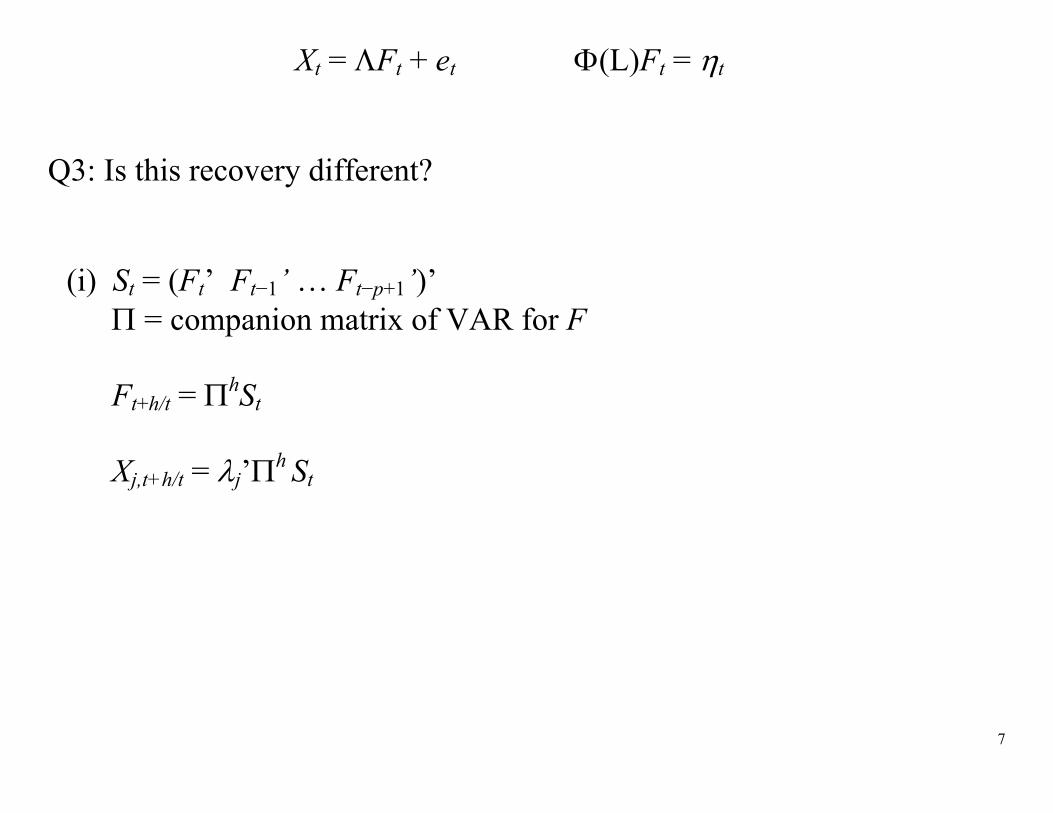
Xt = Ft + et (L)Ft = t Q3: Is this recovery different?
(i) St = (Ft’ Ft−1’ … Ft−p+1’)’ = companion matrix of VAR for F Ft+h/t = hSt Xj,t+h/t = j’h St
8
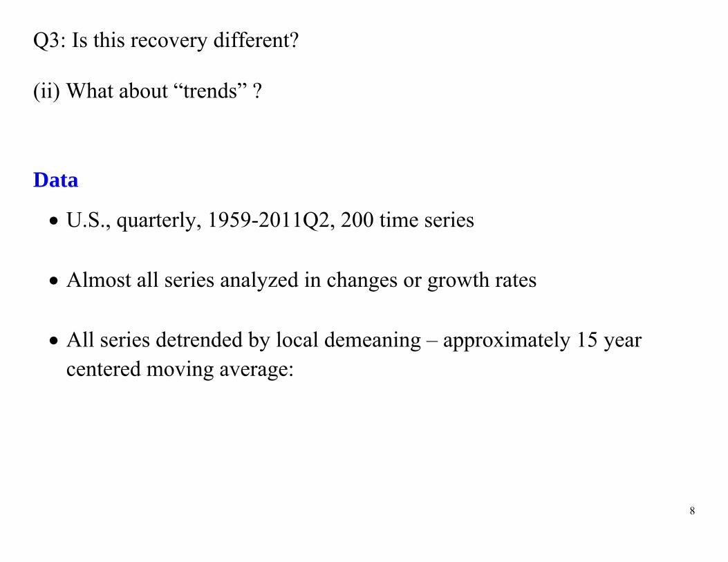
Q3: Is this recovery different? (ii) What about “trends” ?
Data
U.S., quarterly, 1959-2011Q2, 200 time series Almost all series analyzed in changes or growth rates
All series detrended by local demeaning – approximately 15 year
centered moving average:

9
Quarterly GDP growth (a.r.) Quarterly productivity growth
Trend: 3.7% 2.5% 2.3% 1.8% 2.2%

10
Results
1. Structural breaks post 2007Q4 Empirical analysis
1. Estimate DFM parameters using data through 2007Q3 a. Compute factors using “old” factor loadings: b. tF = 1ˆ ˆ ˆ( ) tX , where are pre-07Q3 factor loadings c. How well do pre-07Q3 factors & factor loadings do in explaining
post-07Q4 macro variables?
2. Formal stability tests: a. Stability of b. Test for new factor (excess covariance among idiosyncratic
disturbances)

11
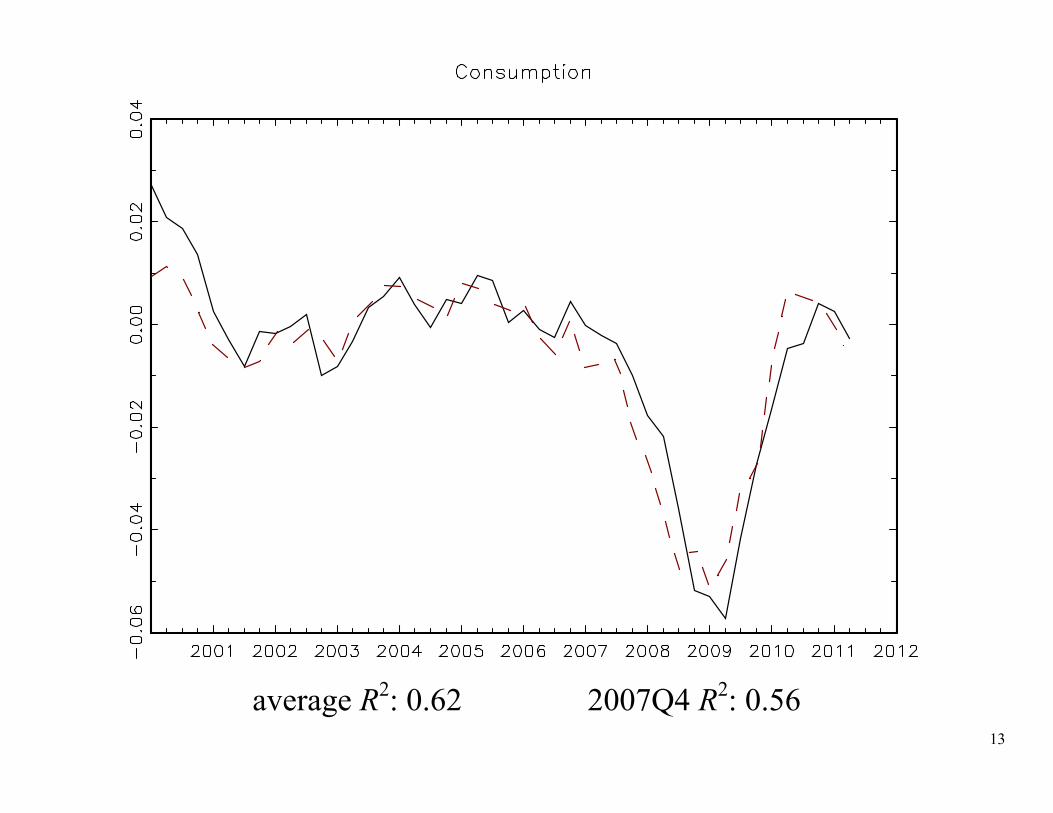
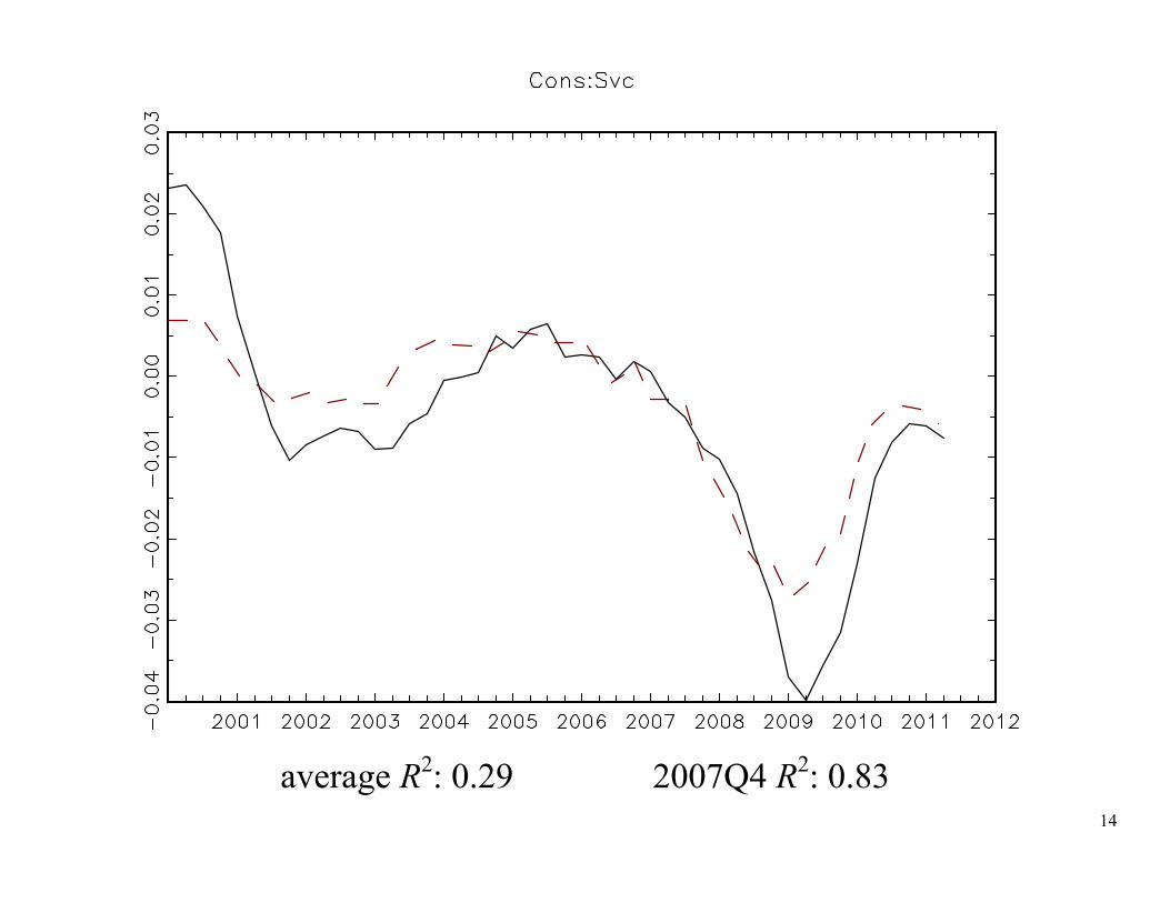
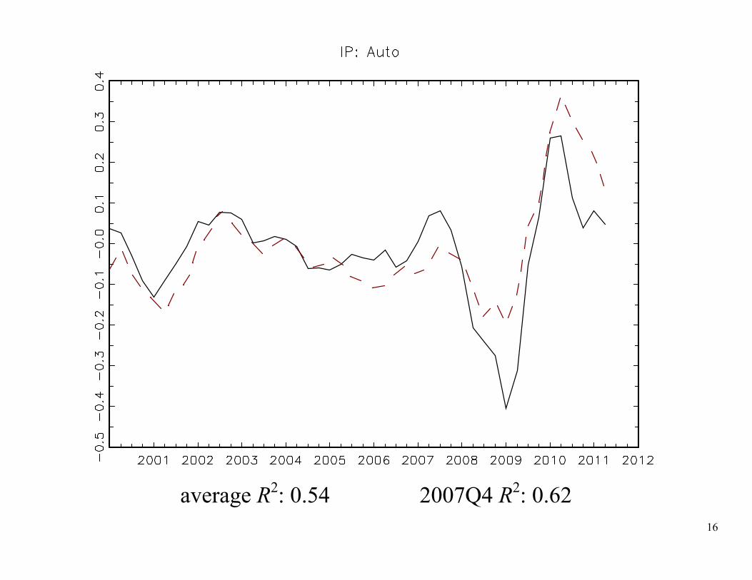
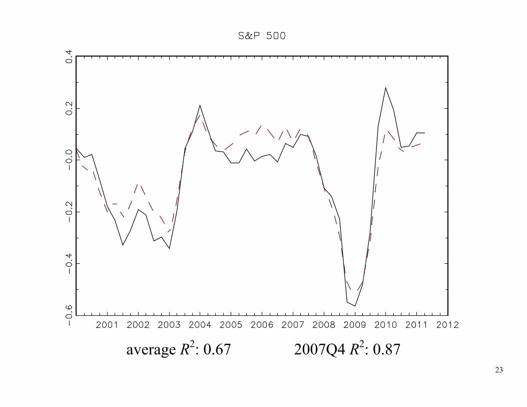
1.1. Fit of pre-07Q3 parameters and factors, post-07Q4 Figures: Plot of 4-Q growth (100ln(Xt/Xt–4)) or 4-Q change: solid = actual dashed = common component (pre-07Q3 model) Average R2 2007Q4 R2 Average R2 = 1-quarter R2 of “Ft”, NBER peak to peak + 14 quarters, averaged over previous 7 recessions, 1960Q1,…, 2001Q1 2007Q4 R2 = value for 2007Q4 – 2011Q2.

12
average R2: 0.78 2007Q4 R2: 0.64
Estimation sample
13
average R2: 0.62 2007Q4 R2: 0.56
14
average R2: 0.29 2007Q4 R2: 0.83

15
average R2: 0.66 2007Q4 R2: 0.86
16
average R2: 0.54 2007Q4 R2: 0.62
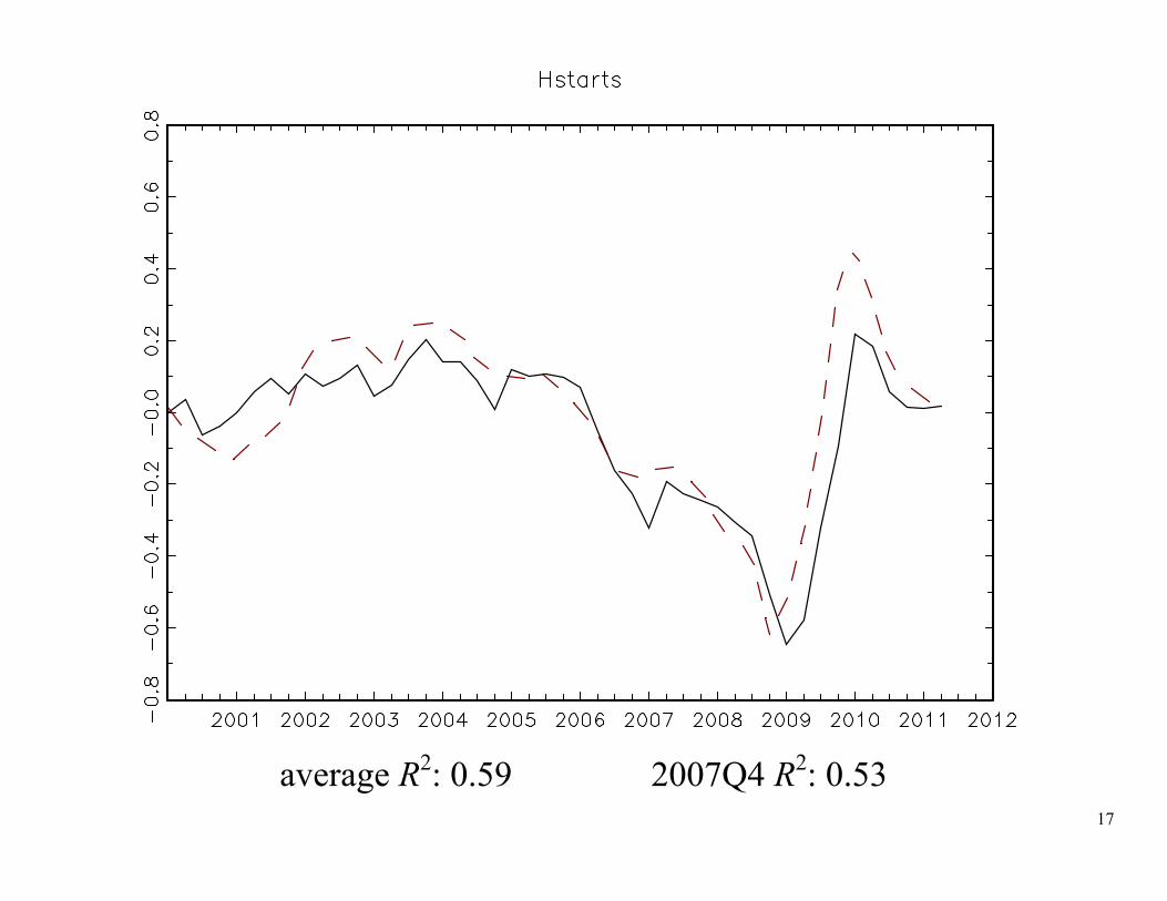
17
average R2: 0.59 2007Q4 R2: 0.53
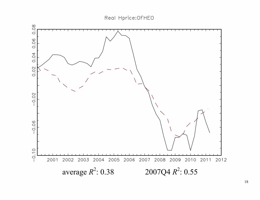
18
average R2: 0.38 2007Q4 R2: 0.55

19
average R2: 0.39 2007Q4 R2: -1.54

20
average R2: 0.22 2007Q4 R2: -0.03
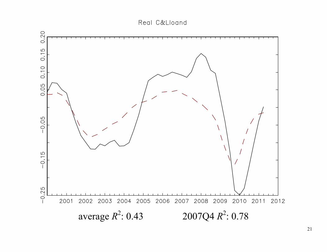
21
average R2: 0.43 2007Q4 R2: 0.78
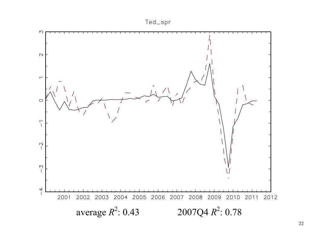
22
average R2: 0.43 2007Q4 R2: 0.78
23
average R2: 0.67 2007Q4 R2: 0.87

24
average R2: 0.12 2007Q4 R2: 0.89
25
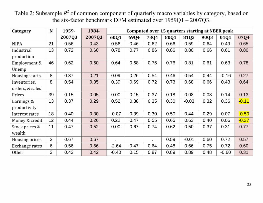
Table 2: Subsample R2 of common component of quarterly macro variables by category, based on the six-factor benchmark DFM estimated over 1959Q1 – 2007Q3.
Category N 1959‐
2007Q31984‐2007Q3
Computedover15quartersstartingatNBERpeak60Q1 69Q4 73Q4 80Q1 81Q3 90Q3 01Q1 07Q4
NIPA 21 0.56 0.43 0.56 0.46 0.62 0.66 0.59 0.64 0.49 0.65 Industrialproduction
13 0.72 0.60 0.78 0.77 0.86 0.86 0.80 0.66 0.61 0.80
Employment&Unemp
46 0.62 0.50 0.64 0.68 0.76 0.76 0.81 0.61 0.63 0.78
Housingstarts 8 0.37 0.21 0.09 0.26 0.54 0.46 0.54 0.44 -0.16 0.27 Inventories,orders,&sales
8 0.54 0.35 0.39 0.69 0.72 0.73 0.68 0.66 0.43 0.64
Prices 39 0.15 0.05 0.00 0.15 0.37 0.18 0.08 0.03 0.14 0.13 Earnings&productivity
13 0.37 0.29 0.52 0.38 0.35 0.30 -0.03 0.32 0.36 -0.11
Interestrates 18 0.40 0.30 -0.07 0.39 0.30 0.50 0.44 0.29 0.07 -0.50 Money&credit 12 0.44 0.26 0.22 0.47 0.55 0.65 0.63 0.40 0.06 -0.37 Stockprices&wealth
11 0.47 0.52 0.00 0.67 0.74 0.62 0.50 0.37 0.31 0.77
Housingprices 3 0.67 0.67 . . . 0.59 -0.01 0.60 0.72 0.57 Exchangerates 6 0.56 0.66 -2.64 0.47 0.64 0.48 0.66 0.75 0.72 0.60 Other 2 0.42 0.42 -0.40 0.15 0.87 0.89 0.89 0.48 -0.60 0.31

26
1.2. Tests: Stability of ? Evidence of a “missing factor”?
Stability of Andrews (1993) end-of-sample stability tests (Table 3) 13% of series reject at 5% level, relative to 1984Q1-2007Q3 ’s Main rejections are in prices, money & credit, interest rates,
housing
27
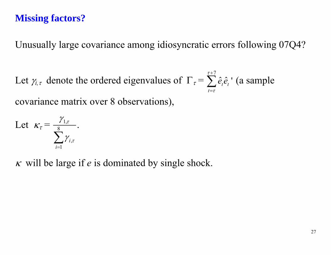
Missing factors? Unusually large covariance among idiosyncratic errors following 07Q4?
Let i, denote the ordered eigenvalues of = 7
ˆ ˆ 't tt
e e
(a sample
covariance matrix over 8 observations),
Let = 1,8
,1
ii
.
will be large if e is dominated by single shock.
28
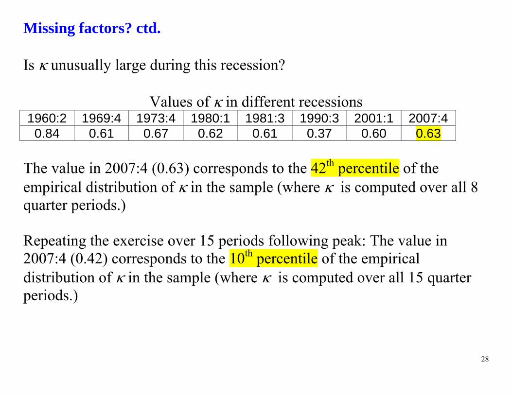
Missing factors? ctd. Is unusually large during this recession?
Values of in different recessions
1960:2 1969:4 1973:4 1980:1 1981:3 1990:3 2001:1 2007:4 0.84 0.61 0.67 0.62 0.61 0.37 0.60 0.63
The value in 2007:4 (0.63) corresponds to the 42th percentile of the empirical distribution of in the sample (where is computed over all 8 quarter periods.) Repeating the exercise over 15 periods following peak: The value in 2007:4 (0.42) corresponds to the 10th percentile of the empirical distribution of in the sample (where is computed over all 15 quarter periods.)

29
Summary: Q1: Stability, new shocks, etc.
from t < 2007Q4 data and 1ˆ ˆ ˆ ˆ( ' ) 't tF X for all t
ˆ ˆ ˆt t tX F e
How does “fit” over t ≥ 2007Q4 compare to t < 2007Q4?
Does te for t ≥ 2007Q4 contain a common shock?
Are and stable across t = 2007Q4?

30
Q2: Which shocks were important during 2007-09?
Innovation in Xjt = j’t = j’Ht

31
Table 5: Innovations to factor components of selected series, by quarter, 2007Q1 – 2011Q2: Standardized innovations
Date GDP Consump- Tion
Invest- ment
Employ- ment
Prod-uctivity
Housing Starts
Oil Price
Fed Funds
Ted spread
VIX Wealth (FoF)
2007Q1 -0.9 -1.3 -0.4 -0.7 -1.2 0.2 1.7 0.3 0.0 -0.6 0.0 2007Q2 0.3 -0.2 0.5 -0.1 0.2 0.8 1.1 0.5 -0.9 -1.4 0.8 2007Q3 -0.3 -0.8 0.0 -0.7 0.0 -0.7 0.3 -0.6 0.7 1.2 -1.0 2007Q4 -0.3 -1.3 0.1 0.3 -0.7 -1.3 1.3 0.4 0.4 0.5 -0.9 2008Q1 -0.3 -0.7 0.1 0.2 -0.4 -1.3 0.2 -0.1 1.4 2.2 -2.0 2008Q2 -1.4 -2.1 -0.4 -1.1 -2.1 1.0 3.4 0.5 0.1 -0.4 -0.8 2008Q3 -1.7 -1.7 -1.0 -0.7 -1.4 -3.5 -0.6 0.2 3.9 2.9 -2.6 2008Q4 1.0 2.1 -0.1 -0.4 4.6 -8.3 -10.3 -2.5 7.7 8.3 -4.1 2009Q1 0.3 -2.7 2.3 0.9 -0.3 -4.7 2.5 3.5 4.0 1.4 -3.3 2009Q2 2.9 1.8 3.3 3.8 0.7 2.9 2.8 3.8 -3.0 -3.4 1.2 2009Q3 1.6 0.4 1.9 2.3 -0.6 4.8 5.0 1.5 -5.2 -3.5 1.5 2009Q4 -1.2 -0.9 -2.0 -2.1 -0.2 0.1 -0.4 -2.1 -1.7 -2.1 2.7 2010Q1 0.3 -0.1 0.6 0.5 0.0 -0.5 0.3 1.2 0.9 0.0 -0.6 2010Q2 0.7 0.3 0.7 0.3 1.3 -2.4 -1.8 0.3 2.1 1.6 -1.2 2010Q3 0.8 -0.3 1.1 0.4 0.9 -1.7 0.0 0.9 1.0 0.3 -0.7 2010Q4 0.3 -0.6 0.6 0.0 0.0 0.6 1.7 0.8 -1.0 -1.8 0.8 2011Q1 0.4 -0.6 1.1 0.5 -0.6 1.5 2.8 1.2 -0.9 -0.8 -0.5 2011Q2 -0.9 -0.8 -1.1 -1.3 -0.6 0.5 0.4 -1.5 -0.7 0.1 0.3

32
What are these big shocks? Digression: SDFM and SVAR identification
(L)Ft = t, t = Hεt,
What is column of H corresponding to “Oil shock”? Strategy: Method of “external instruments”
Use shocks from the literature as instruments. Let KOtZ be Killian
OPEC Oil Supply Shortfall variable (the instrument).
Selected references. Applications: Romer and Romer (1989, 2004, 2008), Ramey and
Shapiro (1998), Ramey (2009) (but they don’t use IV) Methods: Stock and Watson (2008), Mertens and Ravn (2011),
Olea, Stock, and Watson (2012).

33
Method of external instruments, ctd.
Standard approach is to use a constructed exogenous shock series Zt as a regressor – as a shock itself. But in general Zt is only part of the shock, and has measurement error, so including Zt as a regressor (as the shock itself) won’t yield consistent estimation. Instead, treat Zt as an instrument
Assume: (i) Oil KO
t tE Z 0 (Relevance)
(ii) i KOt tE Z = 0 for all other shocks i (Exogeneity)
(iii) E( Oil it t ) = 0 for all other shocks i
Then we can estimate HOil and Oil
t . Note Z can be multidimensional, and this imposed OID.
34
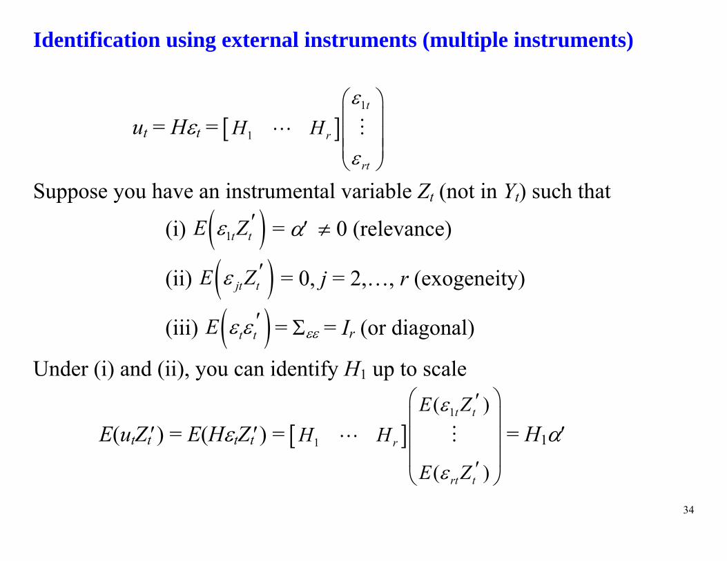
Identification using external instruments (multiple instruments)
ut = Ht = 1
1
t
r
rt
H H
Suppose you have an instrumental variable Zt (not in Yt) such that
(i) 1t tE Z = 0 (relevance)
(ii) jt tE Z = 0, j = 2,…, r (exogeneity)
(iii) t tE = = Ir (or diagonal)
Under (i) and (ii), you can identify H1 up to scale
E(utZt) = E(HtZt) = 1
1
( )
( )
t t
r
rt t
E ZH H
E Z
= H1
35
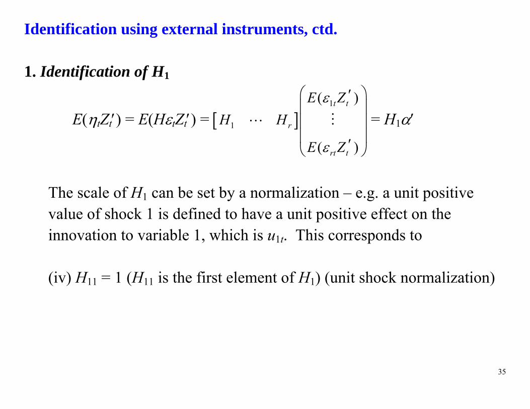
Identification using external instruments, ctd. 1. Identification of H1
E(tZt) = E(HtZt) = 1
1
( )
( )
t t
r
rt t
E ZH H
E Z
= H1
The scale of H1 can be set by a normalization – e.g. a unit positive value of shock 1 is defined to have a unit positive effect on the innovation to variable 1, which is u1t. This corresponds to (iv) H11 = 1 (H11 is the first element of H1) (unit shock normalization)
36
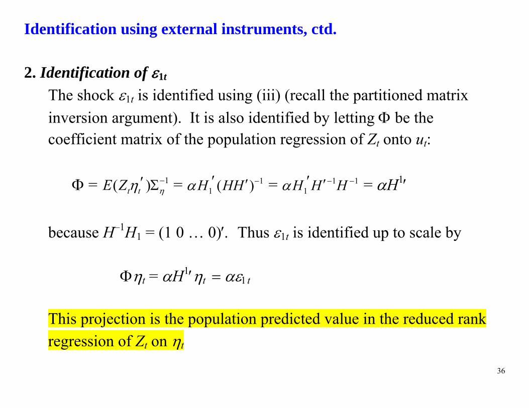
Identification using external instruments, ctd. 2. Identification of 1t
The shock 1t is identified using (iii) (recall the partitioned matrix inversion argument). It is also identified by letting be the coefficient matrix of the population regression of Zt onto ut:
= 1( )t tE Z = 11 ( )H HH = 1 1
1H H H = H1 because H–1H1 = (1 0 … 0) Thus 1t is identified up to scale by
t = H1tt
This projection is the population predicted value in the reduced rank regression of Zt on t
37
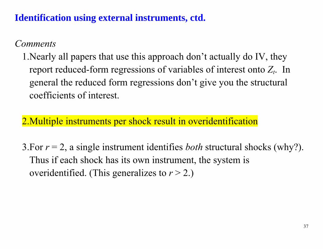
Identification using external instruments, ctd. Comments
1.Nearly all papers that use this approach don’t actually do IV, they report reduced-form regressions of variables of interest onto Zt. In general the reduced form regressions don’t give you the structural coefficients of interest.
2.Multiple instruments per shock result in overidentification
3.For r = 2, a single instrument identifies both structural shocks (why?). Thus if each shock has its own instrument, the system is overidentified. (This generalizes to r > 2.)
38
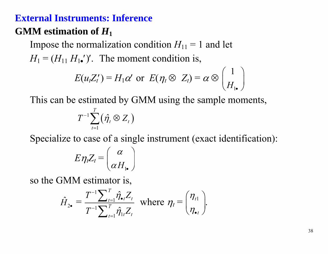
External Instruments: Inference GMM estimation of H1
Impose the normalization condition H11 = 1 and let H1 = (H11 H1)The moment condition is,
E(utZt) = H1 or E(t Zt = 1
1H
This can be estimated by GMM using the sample moments,
1
1
ˆT
t tt
T Z
Specialize to case of a single instrument (exact identification):
EtZt = 1H
so the GMM estimator is,
2H = 1
11
11
ˆ
ˆ
Tt tt
Tt tt
T Z
T Z
where t = 1t
t
.
39
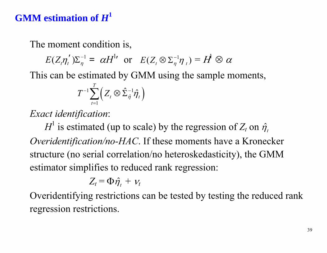
GMM estimation of H1
The moment condition is, 1( )t tE Z = H1or 1( )t tE Z
= This can be estimated by GMM using the sample moments,
1 1ˆ
1
ˆ ˆT
t tt
T Z
Exact identification: H1 is estimated (up to scale) by the regression of Zt on ˆt
Overidentification/no-HAC. If these moments have a Kronecker structure (no serial correlation/no heteroskedasticity), the GMM estimator simplifies to reduced rank regression:
Zt = ˆt + t Overidentifying restrictions can be tested by testing the reduced rank regression restrictions.
40
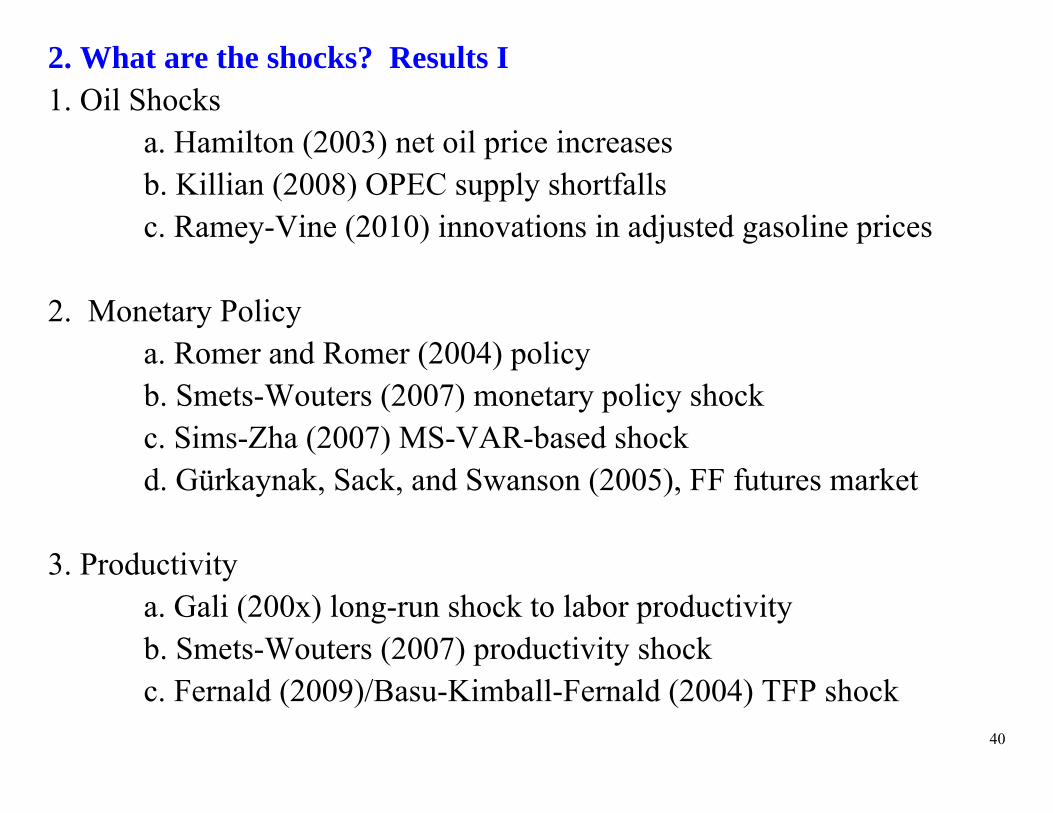
2. What are the shocks? Results I 1. Oil Shocks
a. Hamilton (2003) net oil price increases b. Killian (2008) OPEC supply shortfalls c. Ramey-Vine (2010) innovations in adjusted gasoline prices
2. Monetary Policy
a. Romer and Romer (2004) policy b. Smets-Wouters (2007) monetary policy shock c. Sims-Zha (2007) MS-VAR-based shock d. Gürkaynak, Sack, and Swanson (2005), FF futures market
3. Productivity a. Gali (200x) long-run shock to labor productivity b. Smets-Wouters (2007) productivity shock c. Fernald (2009)/Basu-Kimball-Fernald (2004) TFP shock
41
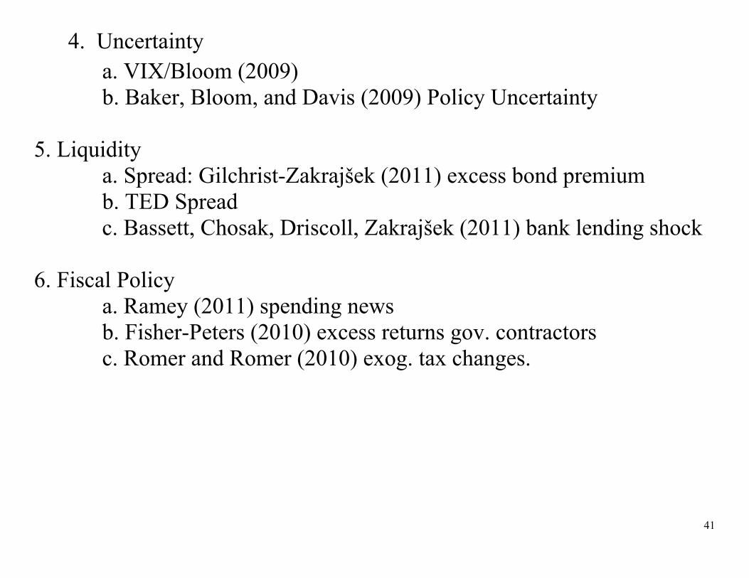
4. Uncertainty a. VIX/Bloom (2009) b. Baker, Bloom, and Davis (2009) Policy Uncertainty 5. Liquidity a. Spread: Gilchrist-Zakrajšek (2011) excess bond premium b. TED Spread c. Bassett, Chosak, Driscoll, Zakrajšek (2011) bank lending shock 6. Fiscal Policy a. Ramey (2011) spending news b. Fisher-Peters (2010) excess returns gov. contractors c. Romer and Romer (2010) exog. tax changes.

42
2. What are the shocks? Results I, ctd. Table 6: Historical importance of shocks Table 7: Correlation matrix of 18 identified shocks Table 8: Contributions of shocks to Post-2007 growth
43
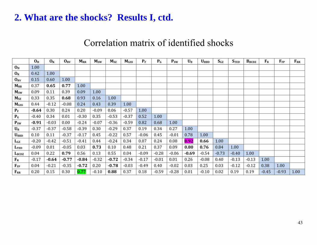
2. What are the shocks? Results I, ctd.
Correlation matrix of identified shocks
OH OK ORV MRR MSW MSZ MGSS PF PG PSW UB UBBD SGZ STED BBCDZ FR FFP FRROH 1.00 OK 0.42 1.00 ORV 0.15 0.60 1.00 MRR 0.37 0.65 0.77 1.00 MSW 0.09 0.11 0.39 0.09 1.00 MSZ 0.33 0.35 0.68 0.93 0.16 1.00 MGSS 0.44 ‐0.12 ‐0.08 0.24 0.43 0.39 1.00 PF ‐0.64 0.30 0.24 0.20 ‐0.09 0.06 ‐0.57 1.00 PG ‐0.40 0.34 0.01 ‐0.30 0.35 ‐0.53 ‐0.37 0.52 1.00 PSW ‐0.91 ‐0.03 0.00 ‐0.24 ‐0.07 ‐0.36 ‐0.59 0.82 0.68 1.00 UB ‐0.37 ‐0.37 ‐0.58 ‐0.39 0.30 ‐0.29 0.37 0.19 0.34 0.27 1.00 UBBD 0.10 0.11 ‐0.37 ‐0.17 0.45 ‐0.22 0.57 ‐0.06 0.45 ‐0.01 0.78 1.00 LGZ ‐0.20 ‐0.42 ‐0.51 ‐0.41 0.44 ‐0.24 0.34 0.07 0.24 0.08 0.92 0.66 1.00 LTED ‐0.09 0.01 ‐0.05 0.03 0.73 0.10 0.48 0.21 0.37 0.09 0.80 0.76 0.84 1.00 LBCDZ 0.04 0.22 0.79 0.56 0.13 0.55 0.04 ‐0.09 ‐0.28 ‐0.06 ‐0.69 ‐0.54 ‐0.73 ‐0.40 1.00 FR ‐0.17 ‐0.64 ‐0.77 ‐0.84 ‐0.32 ‐0.72 ‐0.34 ‐0.17 ‐0.01 0.01 0.26 ‐0.08 0.40 ‐0.13 ‐0.13 1.00 FFP 0.04 ‐0.21 ‐0.35 ‐0.72 0.20 ‐0.78 ‐0.03 ‐0.49 0.40 ‐0.02 0.03 0.25 0.03 ‐0.12 ‐0.12 0.38 1.00 FRR 0.20 0.15 0.30 0.77 ‐0.10 0.88 0.37 0.18 ‐0.59 ‐0.28 0.01 ‐0.10 0.02 0.19 0.19 ‐0.45 ‐0.93 1.00

44
2. What are the shocks? Results II
Contribution to 4-Q GDP growth (1959-2011Q2) of first principal component of two term spread shocks & two uncertainty shocks
45
Q3. Slow Recoveries, 2007Q4 and otherwise
Compute trend and cycle components of recoveries 3.1 Trend As before – approximately 15 year centered MA
3.2 Cycle Different recessionary shocks lead to different recoveries
Xt = Ft + et (L)Ft = t State Vector: (Ft’ Ft−1’ … Ft−3’ )’
Cyclical component: forecast of employment growth, made using factors at the NBER trough

46
3.1 Slow Recoveries: Cyclical component, 1961Q1 – 1980Q3
Quarterly employment growth from NBER troughs, predicted & actual
47
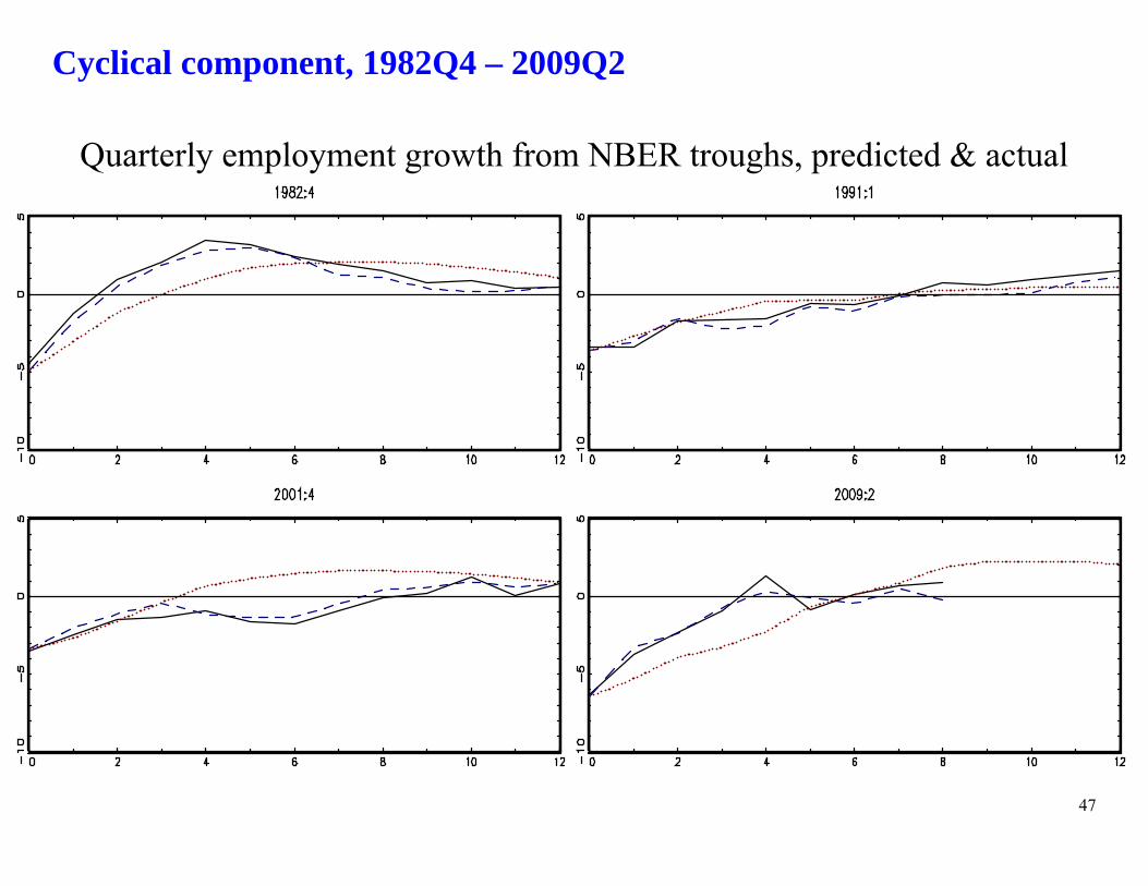
Cyclical component, 1982Q4 – 2009Q2
Quarterly employment growth from NBER troughs, predicted & actual

48
3.2. Slow Recoveries: Trend component
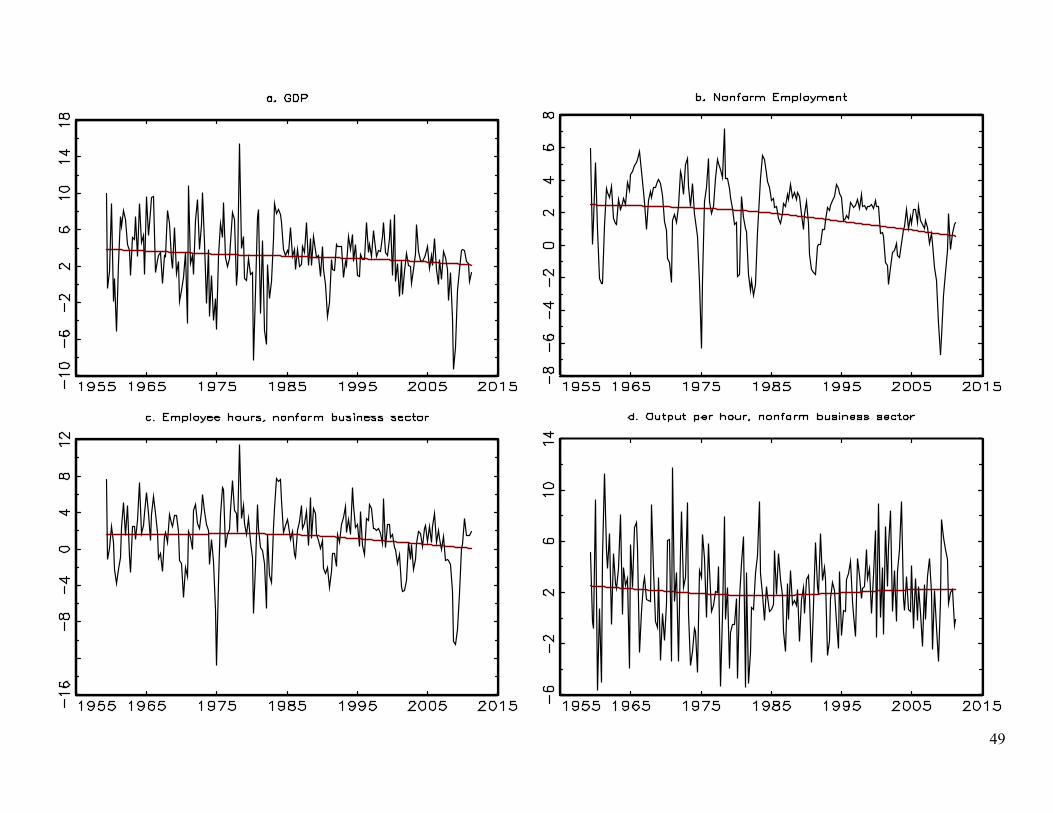
49

50
Table 9 Predicted and actual cumulative growth of output, employment, and productivity
in the 8 quarters following a NBER trough
Trough date Source GDP Nonfarm Employ
ment
Output per Hour (nonfarm business)
1961Q1 Cyclical 1.1 -1.0 2.0 Trend 7.5 4.9 4.8 Total 8.7 4.0 6.8
1970Q4 Cyclical 2.4 0.0 2.6 Trend 6.9 4.7 4.0 Total 9.3 4.6 6.6
1975Q1 Cyclical 3.3 -1.8 5.4 Trend 6.6 4.5 3.7 Total 9.9 2.7 9.1
1980Q3 Cyclical 1.1 -1.5 2.9 Trend 6.3 4.2 3.5 Total 7.5 2.7 6.4
51
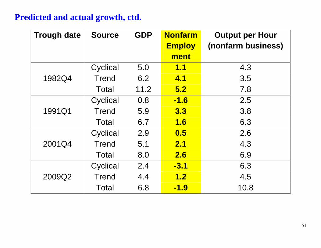
Predicted and actual growth, ctd.
Trough date Source GDP Nonfarm Employ
ment
Output per Hour (nonfarm business)
1982Q4 Cyclical 5.0 1.1 4.3 Trend 6.2 4.1 3.5 Total 11.2 5.2 7.8
1991Q1 Cyclical 0.8 -1.6 2.5 Trend 5.9 3.3 3.8 Total 6.7 1.6 6.3
2001Q4 Cyclical 2.9 0.5 2.6 Trend 5.1 2.1 4.3 Total 8.0 2.6 6.9
2009Q2 Cyclical 2.4 -3.1 6.3 Trend 4.4 1.2 4.5 Total 6.8 -1.9 10.8
52
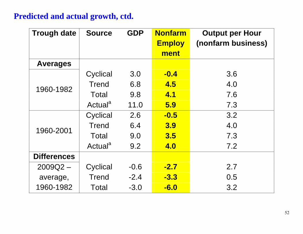
Predicted and actual growth, ctd.
Trough date Source GDP Nonfarm Employ
ment
Output per Hour (nonfarm business)
Averages
1960-1982
Cyclical 3.0 -0.4 3.6 Trend 6.8 4.5 4.0 Total 9.8 4.1 7.6
Actuala 11.0 5.9 7.3
1960-2001
Cyclical 2.6 -0.5 3.2 Trend 6.4 3.9 4.0 Total 9.0 3.5 7.3
Actuala 9.2 4.0 7.2 Differences 2009Q2 – average,
1960-1982
Cyclical -0.6 -2.7 2.7 Trend -2.4 -3.3 0.5 Total -3.0 -6.0 3.2
53
Our interpretation & caveats – Q1
1. The shocks of this recession weren’t new – just bigger versions of things we have seen before.
2. The macro responses to those “old” shocks were the same as they
were historically, given the size of the shocks.
Caveat/issue of interpretation: Structural break analysis limited by sample size (power) There were new shocks (Lehman, TARP, QE) – but it seems that
their (net) effect on macro variables was the same as other financial/uncertainty shocks historically

54
Our interpretation & caveats – Q2
3. Some combination of financial/uncertainty shocks seems to account for most of the recession Caveat
The (structural VAR, and maybe DSGE) literature isn’t ready to identify separately independent financial/uncertainty shocks.

55
Our interpretation & caveats – Q3
4. Slow trend employment growth from demographic shifts underlies slow employment growth from the 2001Q4 and 2009Q2 recoveries. Caveat
Demographic shifts makes trends sound exogenous – but long-term labor supply decisions have endogenous components.