JAISTサマースクール2016「脳を知るための理論」講義03 Network Dynamics
53
SS2016 Modern Neural Computation Lecture 3: Network Dynamics Hirokazu Tanaka School of Information Science Japan Institute of Science and Technology
-
Upload
hirokazutanaka -
Category
Education
-
view
68 -
download
0
Transcript of JAISTサマースクール2016「脳を知るための理論」講義03 Network Dynamics

SS2016 Modern Neural
ComputationLecture 3: Network
DynamicsHirokazu Tanaka
School of Information ScienceJapan Institute of Science and Technology
Neural network as a dynamical system.In this lecture we will learn:• Attractor dynamics
- Hopfield model- Winner-take-all and Winner-less competition• Randomly connectivity
- Girko’s circular law- Phase transition by synaptic variability• Collective dynamics
- Hebb’s cell assemblies- Synfire chain, Neuronal avalanche, small-world network• Recurrent network dynamics
- Echo-state network, liquid-state network- Self-organizing recurrent network (SORN)• Synchronization
- Kuramoto model

Hopfield model inspired by physics of ferromagnetism.
11iS
Hopfield (1982) PNAS; Gerstner (2014) Neuronal Dynamics
“Spin” variable for neuron iExcited
Rest
General connectivity Symmetric connectivity
S1
S2
S3
S4
S5
S6
S7
S1
S2
S3
S4
S5
S6
S7
ij jiw w ij jiw w
Here we will see that a neural network with symmetric connectivity exhibits an attractor dynamics.

Hopfield model inspired by physics of ferromagnetism.
i ij jj
h t w S t
1
1
Pr 1|Pr 1|
i
i
i
i
Si i
Si
h
ti
t
h
S t t h t e eS t t h t ee
H
H
1 tanh
Pr 1|2
i
i i
h t
h t ti
i hi
h teS t t h te e
,
ij i ji j
S w S S H11iS
lim Pr 1| sgni i iS t t h t h t
Hopfield (1982) PNAS; Gerstner (2014) Neuronal Dynamics

Associative memory is stored in connection strengths.
1
1 M
ij i jw p pN
1; 1, , , 1, ,ip i N M
M-stored patterns
Overlap with patterns
1 1 1
1 M N M
i ij j i j j ij j
h t w S p p S p mN
1j j
j
m p SN
Hebbian learning
Hopfield (1982) PNAS; Gerstner (2014) Neuronal Dynamics
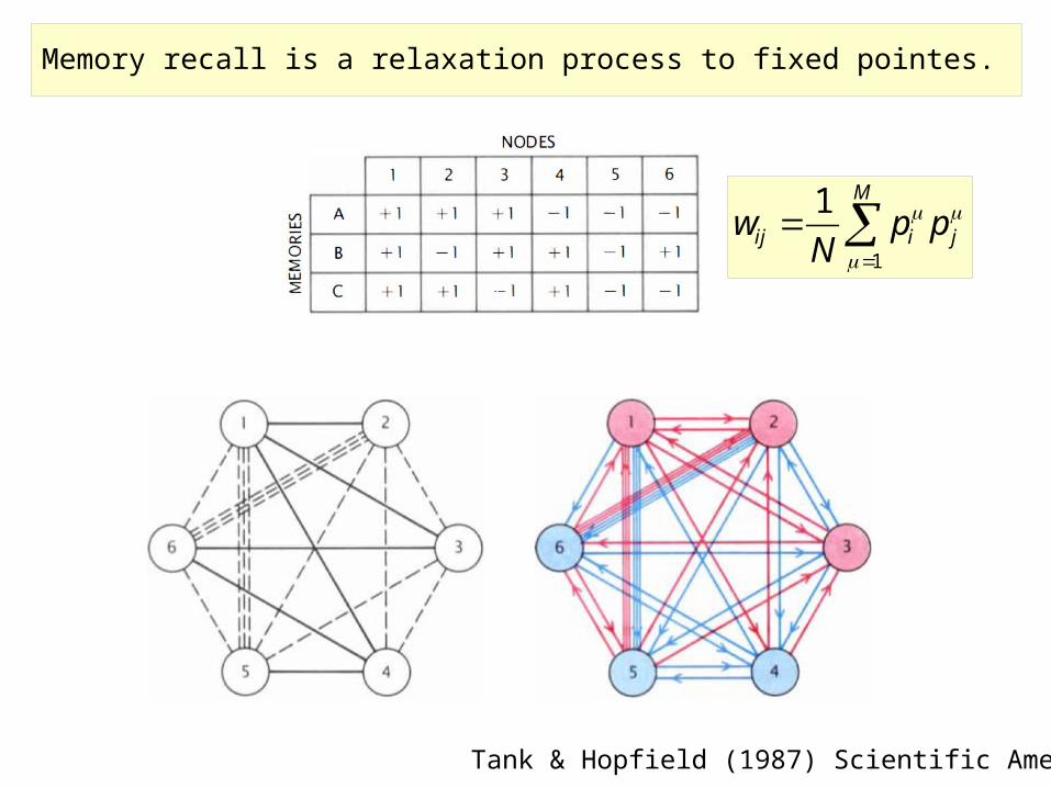
Memory recall is a relaxation process to fixed pointes.
Tank & Hopfield (1987) Scientific American
1
1 M
ij i jw p pN
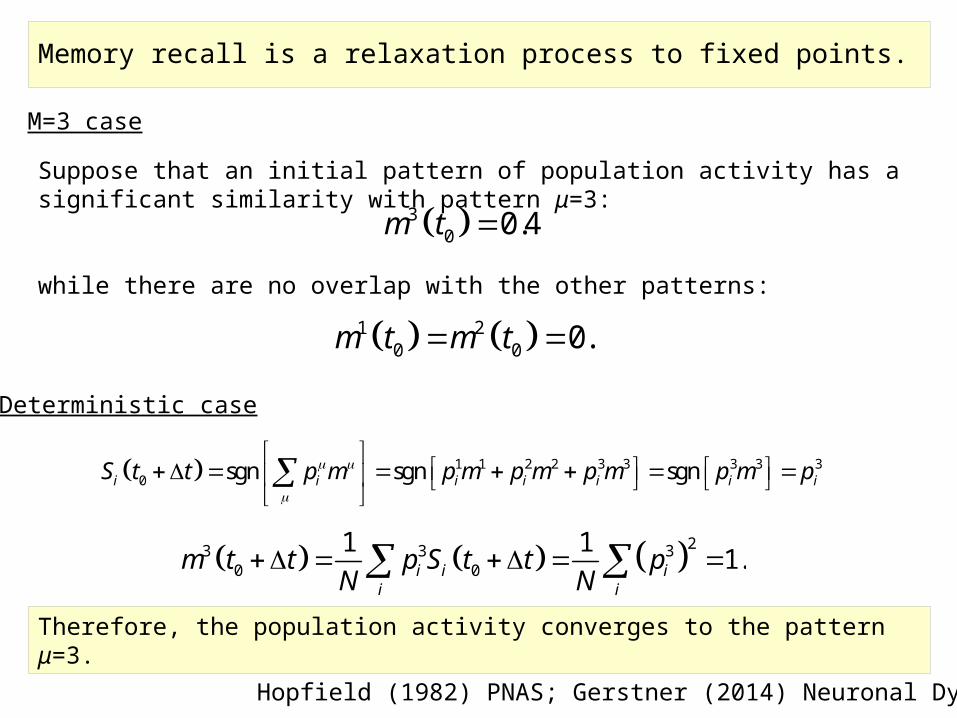
Memory recall is a relaxation process to fixed points.M=3 case
Deterministic case
Hopfield (1982) PNAS; Gerstner (2014) Neuronal Dynamics
Suppose that an initial pattern of population activity has a significant similarity with pattern μ=3:
while there are no overlap with the other patterns:
30 0.4m t
1 20 0 0.m t m t
1 1 2 2 3 3 3 3 30 sgn sgn sgni i i i i i iS t t p m p m p m p m p m p
23 3 30 0
1 1 1.i i ii i
m t t p S t t pN N
Therefore, the population activity converges to the pattern μ=3.
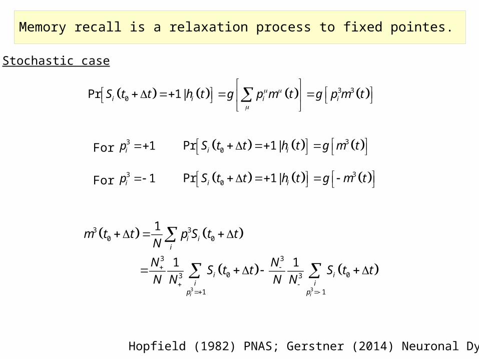
Memory recall is a relaxation process to fixed pointes.Stochastic case
Hopfield (1982) PNAS; Gerstner (2014) Neuronal Dynamics
3 30Pr 1|i i i iS t t h t g p m t g p m t
30Pr 1|i iS t t h t g m t
30Pr 1|i iS t t h t g m t
3 1ip For
3 1ip For
3 3
3 30 0
3 3
0 03 3
1 1
1
1 1
i i
i ii
i ii i
p p
m t t p S t tNN NS t t S t tN N N N
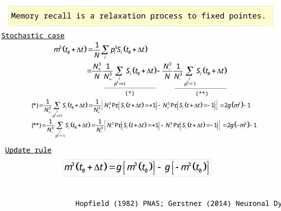
Memory recall is a relaxation process to fixed pointes.Stochastic case
Hopfield (1982) PNAS; Gerstner (2014) Neuronal Dynamics
3 3
3 30 0
3 3
0 03 3
1 1
1
1 1
i i
i ii
i ii i
p p
m t t p S t tNN NS t t S t tN N N N
3
3 3 303 3
1
1 1(*) Pr 1 Pr 1 2 1
i
i i ii
p
S t t N S t t N S t t g mN N
3
3 3 303 3
1
1 1(**) Pr 1 Pr 1 2 1
i
i i ii
p
S t t N S t t N S t t g mN N
3 3 30 0 0m t t g m t g m t
Update rule
(*) (**)

Memory recall is a relaxation process to fixed pointes.
Figure 17,8 in Gerstner (2014) Neuronal Dynamics
3 3 30 0 0m t t g m t g m t
1 1 tanh2
g m m
3 30 0tanhm t t m t
If we assume a sigmoid function for activation:
When β>1, the network is attracted to the pattern.
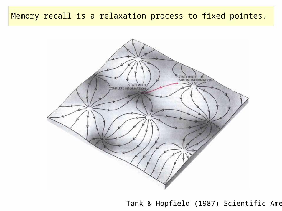
Memory recall is a relaxation process to fixed pointes.
Tank & Hopfield (1987) Scientific American

Demo: Matlab example.
N=25, β=3

Demo: Matlab example.
N=25, β=0.8
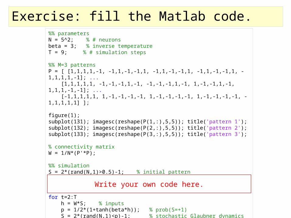
Exercise: fill the Matlab code.%% parametersN = 5^2; % # neuronsbeta = 3; % inverse temperatureT = 9; % # simulation steps %% M=3 patterns P = [ [1,1,1,1,-1, -1,1,-1,-1,1, -1,1,-1,-1,1, -1,1,-1,-1,1, -1,1,1,1,-1]; ... [1,1,1,1,1, -1,-1,-1,1,-1, -1,-1,-1,1,-1, 1,-1,-1,1,-1, 1,1,1,-1,-1]; ... [-1,1,1,1,1, 1,-1,-1,-1,-1, 1,-1,-1,-1,-1, 1,-1,-1,-1,-1, -1,1,1,1,1] ]; figure(1); subplot(131); imagesc(reshape(P(1,:),5,5)); title('pattern 1');subplot(132); imagesc(reshape(P(2,:),5,5)); title('pattern 2');subplot(133); imagesc(reshape(P(3,:),5,5)); title('pattern 3'); % connectivity matrixW = 1/N*(P'*P); %% simulationS = 2*(rand(N,1)>0.5)-1; % initial patternfigure(2); subplot(1,9,1); imagesc(reshape(S,5,5)); title(['t=1']); for t=2:T h = W*S; % inputs p = 1/2*(1+tanh(beta*h)); % prob(S=+1) S = 2*(rand(N,1)<p)-1; % stochastic Glaubner dynamics figure(2); subplot(1,9,t); imagesc(reshape(S,5,5)); title(['t=' num2str(t)]);end
Write your own code here.

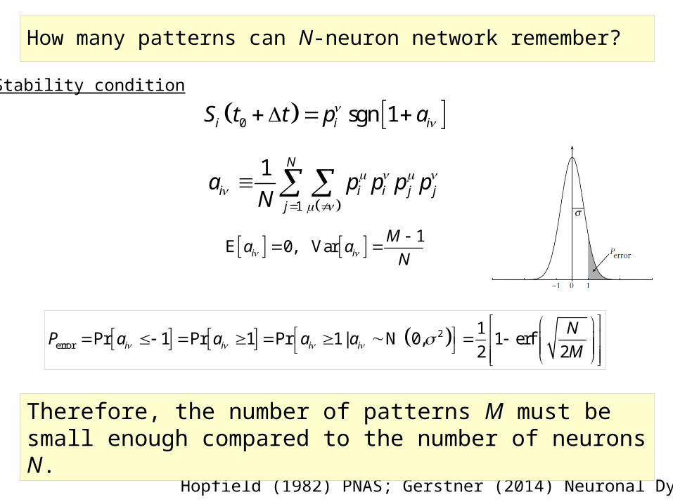
How many patterns can N-neuron network remember?
Hopfield (1982) PNAS; Gerstner (2014) Neuronal Dynamics
Stability condition
0i iS t pAssume that the network represents the pattern ν at time t0:
Then, in deterministic case, the network at time t0+Δt is determined by
01
1 1
1
1
1sgn
1 1 sgn
1 sgn 1
1 sgn 1
N M
i jj
N N
j jj j
N
j
i j
i j i j
i i i j
i
j
S t t p p pN
p p p p p pN N
p p p p pN
pN
1i i
jj
N
jp p p p
How many patterns can N-neuron network remember?
error2 1Pr 1 Pr 1 Pr 1| 1 erf
20
2,i i i i
NP a a a aM
N
Hopfield (1982) PNAS; Gerstner (2014) Neuronal Dynamics
Stability condition
0 sgn 1ii iS t t p a
1
1 N
i ji i jj
a p p p pN
1E 0, Vari iMa aN
Therefore, the number of patterns M must be small enough compared to the number of neurons N.

Physics of spin systems.Ising model
Spin glass
,
i ji j
S J S S H
,
ij i ji j
S J S S H
, : nearest neighbori j
20 ,;ij ij
J JN N
J J
N
,
ij i ji j
S J S S H
Short-range interaction(Edwards-Anderson model)
Long-range interaction(Sherrington-Kirkpatrick model)
Ising (1925); Edwards & Anderson (1975); Sherrington & Kirkpartick (1975)

Simple dynamics with random connections.
tanhddt
x x Wx
2
0,ijWN
N
Nddt
x I W x
Dynamics of N interconnected neural network with random connections
Linearized dynamics
The origin x=0 is a fixed point. Whether it is stable or unstable is determined by the eigenvalues of the connectivity matrix W.
S1
S2
S3
S4
S5
S6
S7

Semi-circle law of eigenvalue density function.10,ij N
W
NAll components are normally distributed:
And symmetric: ij ijW W
Semi-circle law: Wigner (1951)In the limit of infinite n, the eigenvalues of an nxn random symmetric matrix W follow a semi-circle distribution:
21 42
p
%% Parametersn =10000; t =1; v = [ ]; dx = 0.1;%% Experimentfor i=1:t, a=randn(n); % random nxn matrix s =(a+a')/2 ; % symmetrized matrix v =[v ; eig(s)] ; % eigenvaluesendv=v/sqrt (n/2) ; %% Plot[count , x]= hist(v , -2:dx:2) ;cla reset; hold on ;%% Theoryplot(x , sqrt (4-x.^2)/(2*pi) , 'k-', 'LineWidth' , 2);bar (x , count/(t*n*dx) , 'facecolor', [0.7 0.7 0.7]) ;
Wigner (1951)

Circular law of eigenvalue density function.10,ij N
W
NAll components are normally distributed:
Circular law: Girko (1985)In the limit of infinite n, the eigenvalues of an nxn random (not necessarily symmetric) matrix W follow a uniform distribution in a unit circle in the complex plane.
N = 20000;sigma = 1.01;W = randn(N,N)/sqrt(N)*sigma;figure(k); clf; hold on;plot(eig(W)-1, 'k.'); theta = linspace(0, 2*pi, 100);plot(cos(theta)-1, sin(theta), 'k');plot([0 0], [-1 1], 'r')set(gca, 'color', [0.9400 0.9400 0.9400]); axis equal;
Girko (1984) Teor. Veroyatnost. i Primenen.

Circle law of eigenvalue density function.1.00 0.99 1.01

Dale’s law: neurons are either excitatory or inhibitory.
Rajan & Abbott (2006) Phys Rev Lett
Excitatory neuron
inhibitory neuron
0 for ijW i
0 for ijW i
11 1
1
1 1j
n n
i n
ni nj n
W W
W W
W W
W W
W
Exercise: Examine the dynamics of the neural network when Dale’s law is imposed on the random connection matrix, i.e., all components in a column are either positive (excitatory) or negative (inhibitory). This problem is already analyzed by Rajan and Abbott (2006).

Hierarchical modular connectivity structure.
Exercise: Examine the dynamics of the neural network with a hierarchical modular connectivity matrix. This problem has NOT been analyzed so far, to my knowledge.
Anatomical studies suggest that cortical neurons are not randomly connected and that they are connected with a modular and hierarchical manner.
regular network random network small world
HM stochastic HM Cat visual cortex
n×n Hierarchical network:(1) m on-diagonal blocks of size s are connected with prob pm and n=ms.
(2) 1st level of off-diagonal blocks of size s are connected with prob pc.
(3) Subsequent levels of off-diagonal blocks are of size 2s, 4s, 8s, … and connected with prob pcq, pcq2, pcq3, …
Robinson et al. (2009) Phys Rev Lett; Aljadeff, Stern, Sharpee (2015) Phys Rev Lett
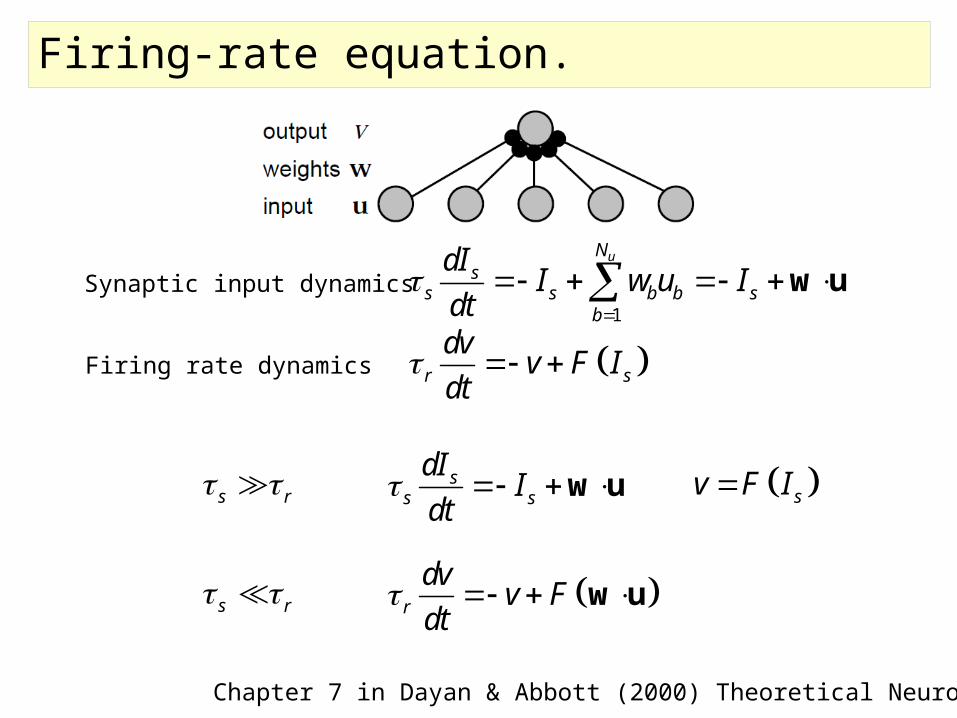
Firing-rate equation.
Chapter 7 in Dayan & Abbott (2000) Theoretical Neuroscience
r sdv v F Idt
1
uNs
s s b b sb
dI I w u Idt
w uSynaptic input dynamics
Firing rate dynamics
s r ss sdI Idt
w u sv F I
s r rdv v Fdt
w u
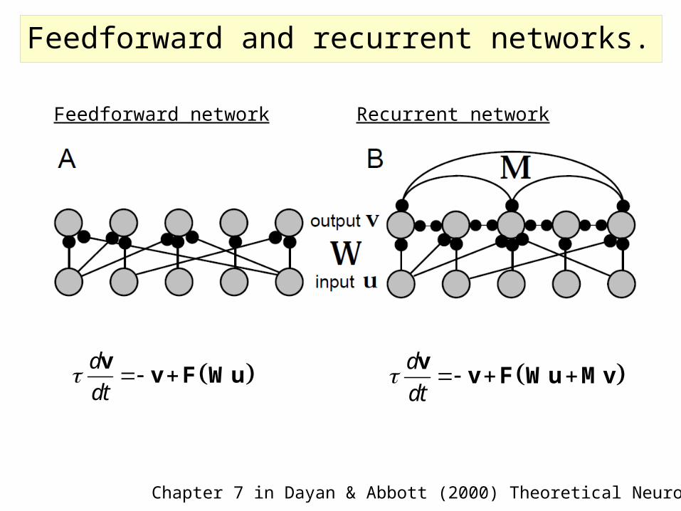
Feedforward and recurrent networks.
Feedforward network
Chapter 7 in Dayan & Abbott (2000) Theoretical Neuroscience
ddt
v v F Wu
Recurrent network
ddt
v v F Wu Mv
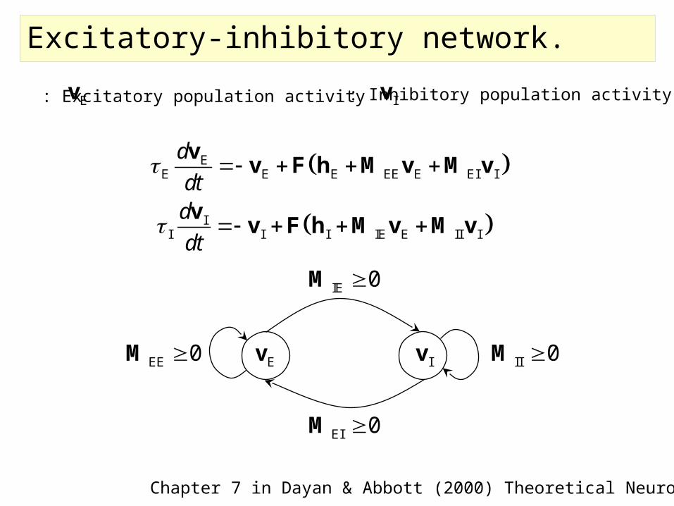
Excitatory-inhibitory network.
EE E E EE E EI I
I I IE E III II
ddtddt
F hv v vM M
F vh M M
v
v v v
Chapter 7 in Dayan & Abbott (2000) Theoretical Neuroscience
Ev IvEE 0M II 0M
IE 0M
EI 0M
: Excitatory population activity : Inhibitory population activityEv Iv

Continuously labeled network.
Chapter 7 in Dayan & Abbott (2000) Theoretical Neuroscience
1 v
T
a Nv v v v Discretely labeled network
Continuously labeled network
v v
11 1
1
v
v v v
N
ab
N N N
M M
MM M
M
,M M
, ,r
dvv F d W u M v
dt

Linear network: Selective amplification.
Chapter 7 in Dayan & Abbott (2000) Theoretical Neuroscience
,r
dvv h d M v
dt
1, cosM

Nonlinear network: Gain modulation.
Chapter 7 in Dayan & Abbott (2000) Theoretical Neuroscience
,r
dvv h d M v
dt
1, cosM

Nonlinear network: Winner-takes-all selection.
Chapter 7 in Dayan & Abbott (2000) Theoretical Neuroscience
,r
dvv h d M v
dt
1, cosM

Nonlinear network: Working memory.
Chapter 7 in Dayan & Abbott (2000) Theoretical Neuroscience
,r
dvv h d M v
dt
1, cosM
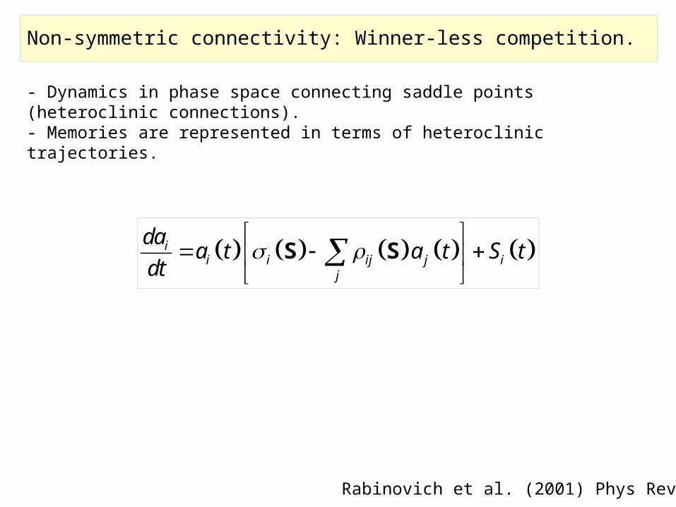
Non-symmetric connectivity: Winner-less competition.
- Dynamics in phase space connecting saddle points (heteroclinic connections).- Memories are represented in terms of heteroclinic trajectories.
ii i ij j i
j
daa t a t S t
dt
S S
Rabinovich et al. (2001) Phys Rev Lett
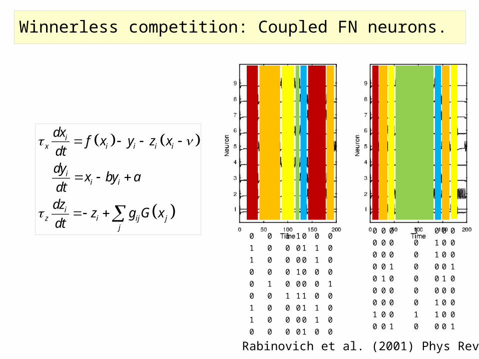
Winnerless competition: Coupled FN neurons.
ix i i i i
ii i
iz i ij j
j
dx f x y z xdtdy x by adtdz z g G xdt
011000110
000010000
100001000
100101000
010001101
011000110
000010000
000000010
000010000
000100001
100000010
011000110
000010000
000100001
Rabinovich et al. (2001) Phys Rev Lett

Winnerless competition: Coupled FN neurons.
ix i i i i
ii i
iz i ji j
j
dx f x y z xdtdy x by adtdz z g G xdt
Rabinovich et al. (2001) Phys Rev Lett
15 52 21 24 45 65 26 36
53 74 57 84 58 86 89 95 2g g gg
g g g g gg g g g g gg
4
2
91
3
5
8
7
6
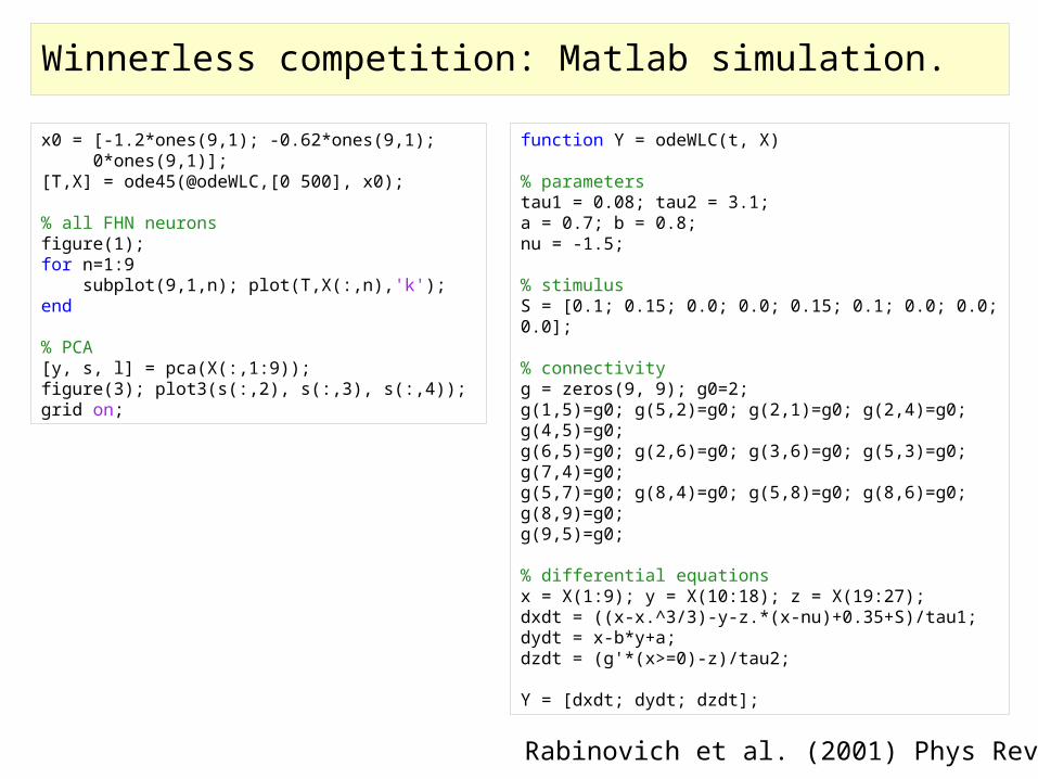
Winnerless competition: Matlab simulation.
Rabinovich et al. (2001) Phys Rev Lett
function Y = odeWLC(t, X) % parameterstau1 = 0.08; tau2 = 3.1;a = 0.7; b = 0.8;nu = -1.5; % stimulusS = [0.1; 0.15; 0.0; 0.0; 0.15; 0.1; 0.0; 0.0; 0.0]; % connectivityg = zeros(9, 9); g0=2;g(1,5)=g0; g(5,2)=g0; g(2,1)=g0; g(2,4)=g0; g(4,5)=g0; g(6,5)=g0; g(2,6)=g0; g(3,6)=g0; g(5,3)=g0; g(7,4)=g0;g(5,7)=g0; g(8,4)=g0; g(5,8)=g0; g(8,6)=g0; g(8,9)=g0;g(9,5)=g0; % differential equationsx = X(1:9); y = X(10:18); z = X(19:27);dxdt = ((x-x.^3/3)-y-z.*(x-nu)+0.35+S)/tau1;dydt = x-b*y+a;dzdt = (g'*(x>=0)-z)/tau2; Y = [dxdt; dydt; dzdt];
x0 = [-1.2*ones(9,1); -0.62*ones(9,1); 0*ones(9,1)];
[T,X] = ode45(@odeWLC,[0 500], x0); % all FHN neuronsfigure(1);for n=1:9 subplot(9,1,n); plot(T,X(:,n),'k');end % PCA[y, s, l] = pca(X(:,1:9));figure(3); plot3(s(:,2), s(:,3), s(:,4)); grid on;

Winnerless competition: Matlab simulation.
Rabinovich et al. (2001) Phys Rev Lett

Example: Olfactory processing in insects.
Mazor & Laurent (2005) Neuron

Cell assemblies: functional units of brain computation.
Definition Cell assembly: a group of neurons that perform a given action or represent a given percept.
Hebb (1949) The Organization of Behavior; Harris (2005) Nature Rev Neurosci

Cell assemblies: functional units of brain computation.
Definition Cell assembly: a group of neurons that perform a given action or represent a given percept.
Hebb (1949) The Organization of Behavior; Harris (2005) Nature Rev Neurosci
1
1
1
1
2
2
2
2
3
3
3
3
4
4
4
4
1
1
1
1
2
2
2
2
3
3
3
3
4 4
44
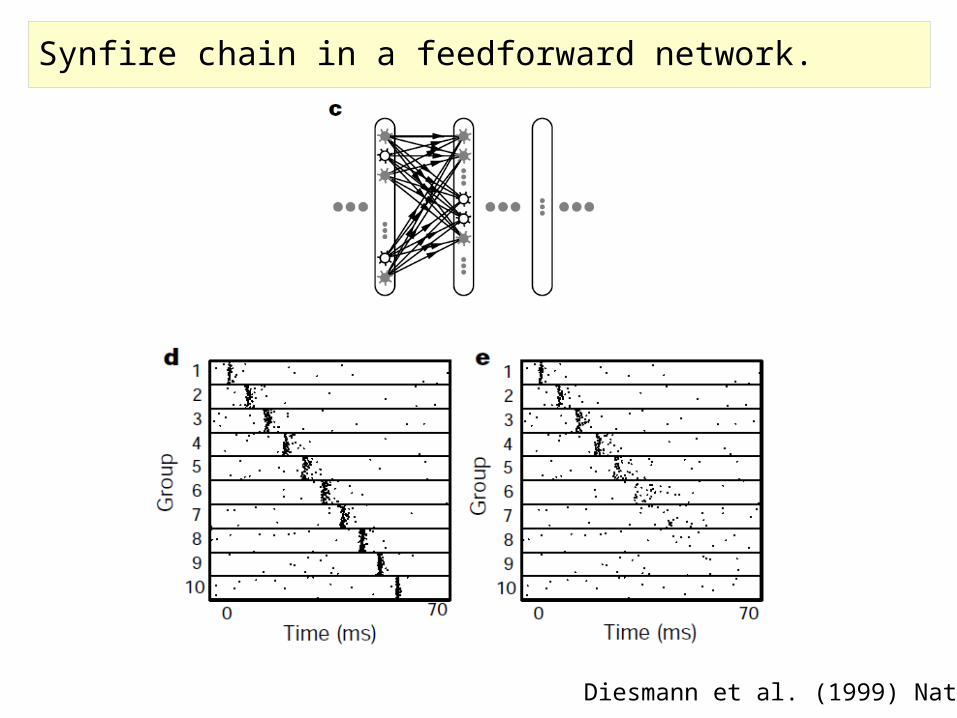
Synfire chain in a feedforward network.
Diesmann et al. (1999) Nature

Synfire chain in a feedforward network.
Brian Spiking Neural Network Simulator,http://briansimulator.org/

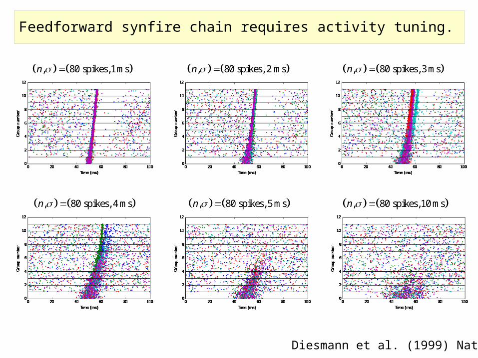
Feedforward synfire chain requires activity tuning.
Diesmann et al. (1999) Nature
, 30 spikes, 2 msn , 40 spikes, 2 msn , 50 spikes, 2 msn
, 60 spikes, 2 msn , 70 spikes, 2 msn , 80 spikes, 2 msn
Feedforward synfire chain requires activity tuning.
Diesmann et al. (1999) Nature
, 80 spikes,1 msn , 80 spikes, 2 msn , 80 spikes, 3 msn
, 80 spikes, 4 msn , 80 spikes, 5 msn , 80 spikes,10 msn

Synfire chain can be made robust by feedback connections.
Moldakarimov et al. (2015) PNAS
1
1
1
1
2
2
2
2
3
3
3
3
4
4
4
4

Synfire chain can be made robust by feedback connections.
Moldakarimov et al. (2015) PNAS
, 80 spikes, 5 msn , 80 spikes, 5 msn , 80 spikes, 5 msn
excitatory feedback: 0.1 excitatory feedback: 0.2 excitatory feedback: 0.3

Neural avalanche with scale-free dynamics.
Beggs & Plenz (2003) J Neurosci 3size where
2P

Neural avalanche as a branching process.
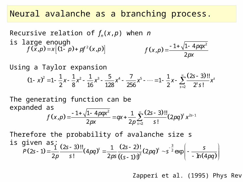
Zapperi et al. (1995) Phys Rev Lett
, , sn n
s
f x p P s p x , ,n ng x p Q p x
21 , 1 ,n nf x p x p pf x p 2
1 , 1 ,n ng x p p pg x p
,nP s p
,nQ p
probability of avalanche of size s
probability of avalanche boundary of size s
Generating function of avalanche size Generating function of avalanche boundary size
Recursive relation of fn(x,p) Recursive relation of gn(x,p)
Neural avalanche as a branching process.
Zapperi et al. (1995) Phys Rev Lett
2, 1 ,f x p x p pf x p 21 1 4
,2
pqxf x p
px
2 2 3 4 5
2
2 3 !!1 1 1 5 7 11 1 12 8 16 128 256 2 2 !
ss
s
sx x x x x x x x
s
2
2 1
2
2 3 !!1 1 4 1, 22 2 !
s s
s
spqxf x p qx pq x
px p s
32
2
2 3 !! 2 2 !1 12 1 4 2 exp2 ! 2 ln 41 !
s ss s sP s pq pq sp s ps pqs
Recursive relation of fn(x,p) when n is large enough
Using a Taylor expansion
The generating function can be expanded as
Therefore the probability of avalanche size s is given as:

Echo-state network: harnessing chaotic units.
Jaeger & Haas (2004) Science
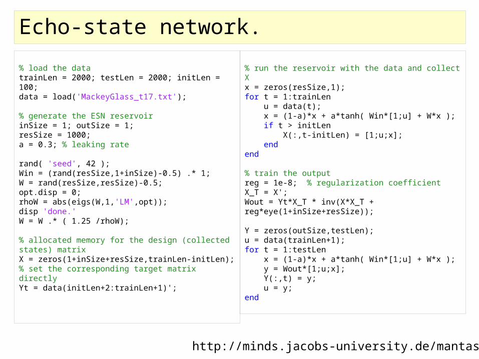
Echo-state network.% load the datatrainLen = 2000; testLen = 2000; initLen = 100;data = load('MackeyGlass_t17.txt'); % generate the ESN reservoirinSize = 1; outSize = 1;resSize = 1000;a = 0.3; % leaking rate rand( 'seed', 42 );Win = (rand(resSize,1+inSize)-0.5) .* 1;W = rand(resSize,resSize)-0.5;opt.disp = 0;rhoW = abs(eigs(W,1,'LM',opt));disp 'done.'W = W .* ( 1.25 /rhoW); % allocated memory for the design (collected states) matrixX = zeros(1+inSize+resSize,trainLen-initLen);% set the corresponding target matrix directlyYt = data(initLen+2:trainLen+1)';
% run the reservoir with the data and collect Xx = zeros(resSize,1);for t = 1:trainLen u = data(t); x = (1-a)*x + a*tanh( Win*[1;u] + W*x ); if t > initLen X(:,t-initLen) = [1;u;x]; endend % train the outputreg = 1e-8; % regularization coefficientX_T = X';Wout = Yt*X_T * inv(X*X_T + reg*eye(1+inSize+resSize)); Y = zeros(outSize,testLen);u = data(trainLen+1);for t = 1:testLen x = (1-a)*x + a*tanh( Win*[1;u] + W*x ); y = Wout*[1;u;x]; Y(:,t) = y; u = y;end
http://minds.jacobs-university.de/mantas/code

Echo-state network.
Summary• Population neural dynamics can be formulated
by using the techniques developed in physics and dynamical systems, including spin models, phase transitions, scale-free dynamics and so on.
• Population activity exhibits a variety of emergent phenomena such as attractor memory dynamics, winner-takes-all process, short-term memory, winner-less competition, and so on.
• Population neural dynamics is a very active field, and a number of novel researches keep going on today.