No.05-E-9July 2005

Inflation Dynamics in China

Ryota Kojima*

ryouta.kojima@boj.or.jp

Shinya Nakamura**

shinya.nakamura@boj.or.jp

Shinsuke Ohyama***

shinsuke.ooyama@boj.or.jp

Bank of Japan2-1-1 Nihonbashi Hongoku-cho, Chuo-ku, Tokyo 103-8660

* Hong Kong Representative Office (formerly of the International Department)** International Department** International DepartmentPapers in the Bank of Japan Working Paper Series are circulated in order to stimulate discussionand comments. Views expressed are those of authors and do not necessarily reflect those of theBank.If you have any comment or question on the working paper series, please contact each author.When making a copy or reproduction of the content for commercial purposes, please contact thePublic Relations Department (webmaster@info.boj.or.jp) at the Bank in advance to requestpermission. When making a copy or reproduction, the source, Bank of Japan Working PaperSeries, should explicitly be credited.

Bank of Japan Working Paper Series

1

Inflation Dynamics in China¶

Ryota Kojima* Shinya Nakamura** Shinsuke Ohyama***

Bank of JapanInternational Department

July 2005

Abstract

This paper comprehensively investigates inflation dynamics in China. First, weestimate a structural vector autoregression to verify the �consensus view� of inflationdynamics in China. We provide the results of basic empirical analyses on inflationmechanisms in China. In the context of the relationship between the output gap and theconventional Phillips curve, we find that the output gap proxied by electricityconsumption per unit of capital is a better measure of inflation pressure than anotheralternative. Based on our analysis of the relationship between input and output prices, weshow that wage growth is a substantial determinant of inflation. The estimation of thelong-run equilibrium relationship between money, output and prices clearly indicates thatthe money gap (i.e., the gap between the actual and long-run equilibrium levels of money)Granger-causes consumer price inflation. Based on these empirical results, we assesscurrent inflation and the outlook for inflation in China and draw policy implications.

¶ We thank staff members of the Bank of Japan, particularly Kumiko Okazaki for constructivecomments from the beginning. We are also grateful to Wataru Hirata, Ryo Kato, Takeshi Kimura,Shigeto Nagai, Yoshihito Saito, Wataru Takahashi, and Kenichiro Watanabe for helpful comments onan earlier draft. Any remaining errors are the authors� own. The views expressed in the paper arethose of the authors and do not necessarily reflect the views of the Bank of Japan.

* Bank of Japan, Hong Kong Representative Office (formerly of the International Department), Email:ryouta.kojima@boj.or.jp** Bank of Japan, International Department, Email: shinya.nakamura@boj.or.jp*** Corresponding author, Bank of Japan, International Department, Email: shinsuke.ooyama@boj.or.jp

2

Nontechnical Summary

This paper comprehensively investigates inflation dynamics and mechanisms in

China since �economic reform and open policies� began in 1978. Section 1 clarifies the

purpose and organization of this paper. Sections 2 and 3 provide an overview of inflation

dynamics in China. Sections 4, 5 and 6 present empirical analyses of inflation

mechanisms and consider the implications of this study and directions for future research.

Section 2 surveys the related literature on inflation in China. Section 3 provides

a historical decomposition of the inflation rate to provide an overview of inflation

dynamics since 1978. China experienced inflation upsurges four times, and inflation

peaked in 1980, 1985, 1988 and 1994. We identify two major factors behind these

inflation upsurges. The first is the influence of price adjustment and liberalization. When

authorities implemented adjustments and reductions in administered prices, inflationary

pressures surged since most administered prices were lower than the market clearing

price levels. The adjustments and reductions in administered prices also fueled inflation

by generating speculative buying and causing opportunistic price increases in consumer

goods. The second factor is the �soft budget constraints� of state-owned enterprises

(SOEs). The SOEs borrowed heavily from the state-owned banks to finance inefficiently

large fixed investments and extreme wage increases, thereby accelerating monetary

growth.

Since 1997, the Chinese economy has not experienced hyperinflation but has

experienced two episodes of deflation, which are negative annual changes in the

consumer price index (CPI). These occurred between 1998 and 1999 and from the end of

2001 to the end of 2002. During these periods, two factors contributed to preventing an

inflation upsurge. The first was the price liberalization, which had been completed in the

mid-1990s. The second was the full-scale reform of SOEs, which �hardened� budget

constrains. In the deflation period of 1998-1999, the main cause of deflation, according

to our results, was a negative demand shock. This was due to the capital crunch (the

banks� reluctance to grant or increase loans) and the fall in household income due to the

reform of SOEs. We find that the increase in supply capacity and the fall in raw-material

prices were the main contributors to the deflation that occurred between the end of 2001

3

and the end of 2002.

The next three sections present empirical studies of inflation mechanisms. In

section 4, we measure the output gap, which is the ratio of actual output to potential

output. Then, we estimate the conventional Phillips curve in order to investigate the

statistical relationship between real-economy fluctuations and the inflation rate. We use

two measures of the output gap. One is the �orthodox� output gap, which is based on the

detrended Solow residual from the production function. The other, referred to as the

�electricity output gap�, uses electricity data to measure the output gap. This measure was

originally proposed by Kamada and Masuda (2000) in their study of Japan�s output gap.

The electricity output gap regards the cyclical component of electricity consumption per

unit of capital as the capital utilization ratio. A comparison of the two output gaps reveals

that the electricity output gap is better than the orthodox measure as the proxy of

inflationary pressure. Based on the estimated Phillips curve, we point out that the

economy overheated in the inflation upsurge periods of 1988 and 1994. We also show

that the output gap has been around zero since mid-2002, while the economy was in

recession in the deflation period of 1998-1999.

Output-price inflation is also affected by the dynamics of input prices. Section 5

analyzes the relationship between input and output prices. Our main findings are as

follows. (1) There is a general tendency for inflation rates to rise with wage increases.

(2) The growth rate of real wages was higher than that of labor productivity before 1997,

but productivity growth exceeded wage growth from 1998. This suggests that relatively

low real-wage growth reduced labor costs and contributed to low inflation after the mid-

1990s. (3) The CPI inflation rate is positively correlated to inflation rates for prices of

raw material and intermediate goods. Therefore, the recent increases in raw-material

prices and intermediate-good prices have put potential upward pressure on consumer

price inflation.

In Section 6, we discuss the empirical relationship between money (M2), output

(real GDP) and prices (the CPI) to complement the previous two sections, in which we

focused on the short-run effects of real-economy fluctuations on inflation. We find a

stable long-run equilibrium relationship between these three variables. More precisely,

the money gap, which is the gap between actual M2 and its equilibrium level relative to

4

output and prices statistically significantly forecast future inflation. That is, money

precedes inflation (or money �Granger-causes� inflation).

Section 7 concludes the paper. Based on the decomposition of inflation and the

output gaps, we conclude that the Chinese economy has been neutral to inflationary

pressure at the end of 2004. Given this finding and given our focus on aggregate data, we

evaluate that the Chinese authorities have controlled the economy well. We also point out

that upward pressure on real wages and the recent increase in raw-material prices and

intermediate-good prices may produce inflationary pressure on consumer prices in the

future. The transition to a market economy in China seems to have strengthened the

flexibility of the economy and the transmission mechanism for monetary policy through

interest rates. Finally, we briefly discuss directions for future research.

5

1. Introduction

China has experienced impressive economic performance since late 2003 when

the economy started to recover from the downturn caused by an outbreak of SARS. Fixed

investment largely increased output growth. The growth rate of real GDP has been more

than 8 percent (per year). Monetary aggregates (such as M2) and the amount of renminbi

bank loans increase by around 15 percent annually. Some people consider these figures to

be the evidence of economic overheating. On the other hand, CPI inflation remains low

and stable. It reached its recent peak of 5.3 percent in July and August 2004, which is low

historically in the context of high-growth periods. Historically, it has been rare in China

for high output growth to accompany low inflation. Therefore, it is difficult to judge the

extent of economic overheating in China in this period.

The purpose of this paper is to improve understanding of China�s economy by

empirically analyzing inflation dynamics in China. Much literature qualitatively discuses

the mechanism behind business cycles in China. By contrast, little empirical work has

been done on China�s economy.1 Several factors explain this paucity of empirical work.

(1) There is limited availability of economic statistics in China. (2) The quality of the

statistics may be dubious.2 (3) Structural changes in the economic system and economic

policies are difficult to control for. However, recently, data availability has increased.

Some economists insist that statistics in China are reliable enough for basic quantitative

analysis.3 Furthermore, it is difficult to disregard the official statistics from the viewpoint

of practitioners in economic research on China. Therefore, we use the official statistics

released by the Chinese authorities for our empirical analysis of inflation.

The remainder of this paper is structured as follows. In Section 2, we present an

overview of inflation development since 1978, when �economic reform and open

policies� began. In Section 3, we decompose the inflation rate into fundamental shocks

by using a structural vector autoregression (SVAR) to identify the causes of inflationary 1 Notable exceptions are Gerlach and Peng (2004), Ha et al. (2003), Oppers (1997) and Zhong (1998).2 For example, Young (2003) argues that real GDP growth in the nonagricultural sector from 1978 to1998 has been overestimated by around 2.5 percent because of an underestimation of the GDPdeflator.3 For example, Professor Gregory Chow (of Princeton University) concludes in Chow (1993) that �Ihave found Chinese statistics, by and large, to be internally consistent and accurate enough forempirical work.�

6

and deflationary episodes. In Section 4, we measure the output gap and estimate the

conventional Phillips curve to quantify the relationship between the output gap and the

inflation rate. In Section 5, we analyze the relationship between the CPI and factor

(input) prices such as labor costs and raw-material prices. In Section 6, we focus on the

long-run relationship between money, output and prices. In Section 7, we provide

concluding remarks.

2. Overview of Inflation Development in China

In 2004, China experienced the favorable combination of high growth (an annual

growth rate of real GDP of 9.5 percent) and low inflation (given an annual CPI inflation

rate of 3.9 percent). This is a rather unusual combination in the context of China�s

history.4 From 1978, the first year of �economic reform and open policies�, to the mid-

1990s, several episodes of pronounced upswings of growth and inflation were followed

by short-lived episodes of relatively low growth and low inflation (Chart 1). The Retail

Price Index (RPI) indicates four inflation cycles, in which inflation peaked in 1980, 1985,

1988 and 1994.5 However, since 1997, when the Chinese authorities introduced market

mechanisms in earnest, China experienced deflation (negative annual growth in the CPI)

twice, from 1998 to 1999 and from the end of 2001 to the end of 2002. At the same time,

the real growth rate fluctuated only between 7 and 9 percent. In this section, we review

these inflation and deflation episodes by conducting a literature survey.

2-1. Mechanisms behind the Inflation Upsurge in the PlannedEconomy

The literature points out the following two factors as the main causes of the

inflation upsurge from 1978 to the mid-1990s. One is the effect of price adjustment and

liberalization. The other is the expansionary expenditure of local governments and SOEs.

4 The People�s Bank of China (2005) has included a column to review inflation dynamics since 1978.5 Since CPI data are only available from 1985, we use RPI data as a proxy for the CPI, followingBrandt and Zhu (2000) and Oppers (1997).

7

2-1-1. Impacts of Price Adjustment and Liberalization

According to Oppers (1997), the following two elements led to an acceleration

of inflation until it peaked in 1980. (1) Price controls were adjusted. (2) Limited

economic reforms were implemented that allowed SOEs to determine some of their own

expenditures. Price adjustment included a large increase in the administered price of

agricultural procurements and the limited introduction of �guided prices�.6 These reforms

led to a sharp increase in aggregate demand because farmers� incomes rose markedly and

SOEs increased investment and wages. Consequently, annual RPI inflation increased

from 1 percent in 1978 to 6 percent in 1980.

Price adjustment and liberalization had been expedited since the mid-1980s by

the so-called �two-track pricing system�, comprising administered prices, guided prices

and market prices. The introduction of market prices caused the prices of daily

necessities to surge and led to an acceleration of RPI inflation in the late 1980s as well as

economic overheating. In April 1988, the authorities implemented a major adjustment in

the administered prices of foods. This led to expectations of further price increases and

speculative buying of durable goods, thereby adding to the strong growth in aggregate

demand. Given an inflation upsurge, further price adjustment and liberalization were

tentatively postponed. In the early 1990s, however, price adjustment and liberalization

accelerated. As a result, most goods on the market have been traded at market prices

since the late 1990s.7 Table 1 clearly indicates a fall in the share of administered prices

and guided prices for retail goods and agricultural products in 1985, 1988 and 1992.

As Gerlach and Peng (2004) pointed out, price adjustment and liberalization are

likely to lead initially to a sharp increase in inflation by causing prices to adjust toward

market-clearing levels and by leading to speculative buying. Prices decline in the long

run as competition in the deregulated market leads to a more efficient allocation of

resources and lower profit margins.

6 Administered prices are controlled by the central or provincial authorities. Guided Prices fluctuatewithin a band set by the authorities.7 As Oppers (1997) points out, �market prices� are not necessarily fully determined by the market,because there has been intervention in the form of price management and indirect controls.

8

2-1-2. Rising Expenditures of Local Governments and SOEs

Much previous work suggests that the rising expenditure of local authorities and

SOEs during the process of decentralization was one of the main contributors to business

cycles in China. For example, greater autonomy for SOEs in setting wages and allocating

social funds is thought to have been one of the main causes of the economic overheating

and inflation upsurges of 1985 and 1988 because it led to large wage increases and

inefficiently large fixed investments.

The soft budget constraints of publicly owned enterprises account for inflation

upsurges driven by excessive fixed investment by local authorities and SOEs.8 Fan

(2003) explains that a company faces a soft budget constraint if it cannot go bankrupt

because of ex post compensation by the authorities (or state-owned banks). A soft budget

constraint induces local authorities and SOEs to expand their expenditure as much as

possible. Therefore, once restrictions on liquidity and fixed investments are relaxed,

local authorities and SOEs compete to expand their expenditures, and this generates

inflationary pressures.

Brandt and Zhu (2000, 2001) explain how soft budget constraints accelerate

inflation as follows. When credit allocation is decentralized from the central government

to local governments, state-owned banks can divert loans from inefficient SOEs to the

more productive non-state sector. While this diversion increases fixed investment and

production in the non-state sector, the share of SOEs in total output declines. However,

since governments commit to the investment and employment of SOEs, governments

must transfer funds to SOEs. They provide funds in the form of cheap credit from the

state-owned bank and money creation to finance wage payments, capital expenditures

and other costs.9 Local governments that are responsible for promoting local economic

growth also force local branches of the central bank to expand their loans to state-owned

banks.10 Hence, actual credit exceeds the credit level set by the central government. The 8 Zhong (1998, 2003) surveys the models to explain the relationship between the expenditures of localgovernments and SOEs and business cycles.9 Consequently, the gap between the output contribution of the SOEs and their shares of employmentand investment increased.10 Ma (1995) explains why local branch offices of the central bank are controlled by local governments.One reason is that the central bank is not allowed to nominate a branch manager without localgovernment consent. Another is that executive promotions are based on contributions to localeconomic growth.

9

central bank relies increasingly on money creation to finance increasing transfers.11

Consequently, aggregate demand increases, there is overheating, and inflation accelerates.

In other words, when SOEs have soft budget constraints, China�s economy booms

because quantitative controls on investment and credit are relaxed.

In Chart 2, we illustrate trends in seigniorage, money (M2) and the CPI.12

Seigniorage tends to precede money and inflation until the mid-1990s. This observation

is consistent with the mechanism described above.

We summarize the previous arguments as follows. The two factors that caused

the inflation upsurges of 1980, 1985, 1988 and 1994 were: (1) price adjustment and

liberalization, which generated a negative supply shock in the short run; and (2) money

creation due to the soft budget constraints of SOEs, which generated a positive demand

shock.

2-2. Determinants of Inflation in the Transition to a Market Economy

China�s economy has had no inflation upsurges since 1995 but has experienced

deflation twice: once from 1998 to 1999, and again from the end of 2001 to the end of

2002. The transition to a market economy affects the inflation mechanism. The reform of

SOEs started in the 1970s but accelerated from late 1996. The reform was equivalent to a

reduced commitment by central government to SOEs, and it hardened the budget

constraints of SOEs. This made it harder to finance rising state-sector expenditure by

printing money. Market forces weeded out inefficient SOEs to normalize the balance of

aggregate demand and supply in China�s economy. At the same time, state-owned banks

were reformed to reduce and restrain nonperforming loans. This blocked the mechanism

of amplifying inefficient credit growth. As a result, it became somewhat easier for

authorities to avoid economic overheating.

The hardening of SOEs� budget constraints reduced inflation but did not

necessarily cause deflation. Fan (2003) insists that the capital crunch (banks� reluctance

11 Brandt and Zhu (2000) estimate that more than 3 percent of GNP was transferred annually to SOEsto support their management in 1993.12 Seigniorage and money are calculated as annual increases in M0 and M2 (as shares of nominal GDP,detrended) following Brandt and Zhu (2000).

10

to grant or expand loans) reduced aggregate demand growth and caused deflation at the

end of the 1990s. In fact, the growth of bank credit slowed from late 1996 to late 2002

(Chart 3). By contrast, Fan (2003) and Feyzioglu (2004) attribute the deflation from the

end of 2001 to 2002 to improvements in economic efficiency and the rise in factor

productivity. We measure the growth of labor productivity as the growth of per capita real

output (Chart 4). The fact that the growth rate of per capita GDP has risen since 1998

indicates the existence of positive supply shocks. In addition, Feyzioglu (2004) points to

the decline in raw-material prices and the reduction in tariff rates as common features of

the two deflationary periods.

Chart 5 shows the decomposition of annual CPI inflation into its components.

We assume that the component weights of the CPI after 2001, the year of major statistical

revision, are the same as those of 2004, while weights for years before 2000 are set equal

to 1995 weights. We identify the following characteristics.

(1) The behavior of both the CPI, including and excluding foods, changed

dramatically before and after 1997.

(2) Foods is the main contributor to CPI dynamics, since it has the largest

weight in the components.

(3) Most components rose in 1994, which suggests the influence of a positive

demand shock.

To summarize, the reform of state-owned enterprises contributed to dampening

the positive demand shock. In other words, the main determinants of inflation dynamics

changed in the mid-1990s. Thus, we investigate inflation mechanisms empirically in the

following four sections.

3. Decomposition of Inflation Development based on a Structural VAR

In this section, we investigate the shocks driving inflation in China. For this

purpose, we estimate a bivariate SVAR for the growth rates of real GDP and the CPI in

order to decompose inflation dynamics since the late 1980s into two components,

aggregate demand shocks and aggregate supply shocks.

11

For the identification of the model, we assume that an aggregate demand shock

has no long-run impact on the level of output. Zhang (2003) applies this approach to

Chinese data.13 She begins by calculating real output by deflating monthly industrial

production by the GDP deflator. Then, she estimates an SVAR on monthly data for real

output and the RPI. She concludes that aggregate demand shocks primarily explain

inflation in China. We estimate a quarterly SVAR for real GDP and CPI inflation by

using data from 1987 and empirically examine the discussion of the previous section.14

We first check for unit roots and cointegration between real GDP and CPI to

confirm that both time series follow I(1) processes and are not cointegrated. Then, we

estimate a reduced form VAR comprising the first differences of the two variables.15 We

identify the parameters of the SVAR by imposing the long-run restriction that aggregate

demand shocks have no long-run impact on output levels.16

Chart 6 presents identified cumulative impulse responses for real GDP and CPI.

Both impulse responses for real GDP are compatible with the signs expected from

economic theory. However, while economic theory predicts a negative long-run response

of CPI to aggregate supply shocks, the impulse response changes from negative to

positive four quarters after the shock. The variance decomposition in Table 2, however,

indicates that aggregate demand shocks primarily explain inflation fluctuations: they

explain 91.1 percent after four quarters and 69.6 percent after 36 quarters. This result

implies that even if the long-run response of CPI to aggregate supply shocks is not of the

expected sign, it would have a negligible impact in the context of the historical

decomposition.17

Chart 7 depicts the contributions of aggregate demand and supply shocks to

inflation. In the inflation cycle that peaked in 1994, demand shocks contribute to the rise

13 Zhang (2003) refers to Liu and Zhang (2002, which is in Chinese and not available to the authors),who estimate an SVAR by using quarterly data. According to Zhang (2003), their work has thefollowing shortcomings relating to the data used. (1) The data are accumulated from the beginning ofthe year. (2) Missing data on nominal GDP are replaced by data on industrial production.14 Data are from 1987Q1 to 2004Q4. Both real GDP and the CPI are seasonally adjusted on the basisof an X-12-ARIMA model.15 We set the lag length at three, a priori. The results are robust to changes in the lag length of theVAR.16 We estimated the model by indirect least squares.17 This argument follows Mio (2001).

12

in inflation. This feature coincides with the positive demand shock under soft budget

constraints, in the form of the rising fixed investment and wage increases of SOEs and the

accompanying increases in monetary aggregates. The component explained by the

supply shock also increases from 1993 to 1994. This is consistent with the argument of

the previous section that price adjustment and liberalization initially worked as a negative

supply shock to rise inflation.

In marked contrast to the movement before 1996, the component explained by

the demand shock does not increase significantly after 1997. This supports the

hypothesis that the budget constraints of SOEs hardened following reforms to introduce

the market mechanism in China from 1996. It is also clear that the driving forces behind

the two deflationary episodes are qualitatively different. In the former period, from 1998

to 1999, the negative demand shock caused deflation. This coincides with the argument

of Fan (2003) that the capital crunch was the main source of deflation. Another candidate

for a negative demand shock is the wage reduction accompanied by the structural reform

of SOEs. By contrast, the positive supply shock (reflecting the improvement in overall

economic efficiency) drove the inflation rate below zero in the second deflationary period,

from the end of 2001 to the end of 2002.

The preceding empirical results and the arguments of the previous section

suggest the following. First, the determinants of inflation changed in 1996, when the

reform of SOEs and state-owned banks began in earnest. Second, given that large

increases in positive demand shocks are rare, the positive supply shock, in the form of

increased capacity, has contributed the recent low levels of inflation. These results also

imply that China�s economy has been more market oriented recently. Hence, in the

following three sections, we discuss three relationships that are important for the market

economy. These are the relationship between the output gap and inflation, the

relationship between input (factor) and output prices, and the long-run relationship

between money, output and prices.

4. The Output Gap and the Conventional Phillips Curve

In this section, we measure the output gap, i.e., the gap between actual and

13

potential output, and investigate its influence on inflation. There are two broad

approaches to measure output gaps. One is the production function approach. In this

approach, one constructs a production function comprising capital, labor and total factor

productivity (TFP). One can then estimate potential output as the average of those three

factors.18 An advantage of this approach is that it provides information on the sources of

economic growth, while mismeasuring capital and labor may bias the estimated output

gap.

Another approach is to estimate potential output from the trend in real GDP by

using time-series techniques. While this approach avoids the effect of measurement

errors in factors, the dynamics of potential output must be known a priori. This method

also provides no information on growth mechanisms. Thus, it is often considered as a

complement to the production function approach.

We first estimate and compare two output gaps with the production function

approach by using annual data from 1978 to 2004. One is the orthodox output gap and the

other is the electricity output gap, based on electricity data. This measure was originally

proposed by Kamada and Masuda (2000) in their study of Japan�s output gap. Then, we

estimate the output gap by using time-series techniques with quarterly data from 1987Q1

to 2004Q4. Then, we review the development of inflation from the late 1980s based on

these output gaps.

4-1. The Output Gap based on the Production Function Approach

4-1-1. The Orthodox Output Gap

We first estimate the orthodox output gap ( orthgap ) by using the production

function approach.

The first step is to set up a Cobb�Douglas production function comprising

capital, labor, and TFP, following Chow (1993) and Chow and Li (2002):

( ) αα γ −⋅⋅⋅= 1KLAY (1)

18 There are two definitions of potential output. One defines potential output as the maximum level ofoutput that a country can produce. The other defines it as an average level of output. In this paper, weadopt the latter definition.

14

where Y is real output, A is TFP, L is labor input, K is capital stock, γ is the capital

utilization ratio, the average of which is set to unity, and α is the labor contribution ratio.

Under the assumption of perfect competition, α is equal to the labor distribution ratio.

Taking logarithms of both sides of equation (1), we have the following.

( ) ( )KLAY ⋅−++= γαα ln1lnlnln (2)

The Solow residual ( Aln ) is derived by subtracting the second and third terms on the

right-hand side from the left-hand side of equation (2).

Potential output is the output level produced with the average amounts of labor,

capital, and the capital utilization ratio (which is unity).

( ) KLAY ln1lnlnln ** αα −++= (3)

The output gap is defined as the difference between actual and potential output. Equation

(4) represents the basic definition of the output gap.

( ) ( ) γαα ln1lnlnlnln ** −+−=−≅ LLYYgap (4)

Next, we describe the data used to estimate the output gap (see the Appendix for

details). Y is real GDP and L is total employment. K is the capital stock, as originally

estimated by Chow (1993) and extended by authors using the method of Chow and Li

(2003). α is the average labor contribution from 1993 to 2003.19

The disadvantage of the production function approach is that the quality of the

estimates depends heavily on data quality. There are no data in China that can be used to

measure γ . Kamada and Masuda (2000) point out that even if data for γ contains

measurement error, one can obtain unbiased estimates of TFP and the output gap by

regressing Aln on a linear time trend under two conditions. That is, γln must equal zero

on average, and true TFP growth must be constant. Hence, we assume that TFP increases

with a linear trend (i.e., tA ⋅+= 21ln ββ , so that 121ln etA +⋅+= ββ ) and that γ is

fixed at unity.20

19 We obtain similar results when we use 60.0=α , which is the average value of the laborcontribution from 1978 to 1995 used in Young (2003).20 We have not seen the early studies on potential GDP or on the GDP gap in China in which theutilization of capital is adjusted.

15

It is questionable whether *L , total employment, is an appropriate proxy for true

labor input. According to Marukawa (2002), labor statistics in China may be dubious for

two reasons. First, the coverage of unemployment is much more restrictive than the

international standard. Second, employees who are laid off are not defined as

unemployed. For example, the unemployment rate in China fluctuates little although real

GDP growth suggests business cycles since 1978. Furthermore, the unemployment rate

has been rather stable recently although unemployment in urban areas is being treated as a

serious social problem. Thus, we suggest that, at best, data on total employment merely

represent the trend in labor input but do not reflect precise fluctuations in labor input. In

other words, total employment may measure labor input with error. According to

Kamada and Masuda (2000), one can obtain unbiased estimates of TFP and the output

gap by regressing Aln on a linear time trend if the following two conditions are satisfied.

First, *lnln LL − is zero on average. Second, true TFP follows a linear time trend. Hence,

we assume that *lnln LL − is always zero and TFP follows a linear trend.

The assumptions of a linear time trend for TFP, a constant γ , and *LL = imply

that the orthodox output gap is equivalent to the residual from a regression of Aln on a

linear time trend.

1*lnln eYYgaporth =−≅ (5)

where AAe lnln1 −= .

Chow (1993) assumes that TFP was constant before 1978, the first year of

�economic reform and open policies�, and has since increased on a linear trend.

Following Chow (1993), we assume the linear time trend is zero before 1978 and

increases by one each year thereafter.

4-1-2. The Electricity Output Gap

In estimating the orthodox output gap, we controlled for the influence of

fluctuations in capital utilization by assuming a linear trend for TFP. Here, we estimate

the capital utilization ratio directly from electricity consumption data and incorporate this

in measuring the output gap.

Statistics on electricity consumption and production are compiled by the central

16

government. Wang and Meng (2001) list the following conditions for the reliability of

statistics in China. First, statistics should not be compiled by local governments because

they have incentives to exaggerate the results of their economic policies. Second,

statistics should not be deflated by price indices but should be measured in real terms.

Electricity statistics satisfy these criteria.

Kamada and Masuda (2000) originally proposed measuring the capital

utilization ratio by using electricity data in the context of measuring the output gap. Their

basic idea is as follows. The trend component of electricity consumption per unit of

capital is considered to be determined by industry structure and the technology embodied

in capital. Thus, the cyclical component corresponds to capital utilization.

Following Kamada and Masuda (2000), we measure the output gap in China by

using electricity data. We first calculate electricity consumption per unit of capital by

dividing electricity production by the capital stock and assuming that this follows a linear

trend.

221 etKELEC +⋅+= µµ (6)

where ELEC is electricity production.

The first and second terms on right hand side of equation (6), t⋅+ 21 µµ ,

represents the electricity consumption per unit of capital corresponding to potential

output. This decreases if the overall energy efficiency of the economy improves, while it

increases when the proportion of high-energy-consuming industries increases. It also

increases if electricity is substituted for coal and as household use of air conditioners

spreads. In Chart 8, the electricity consumption per unit of capital, KELEC , levels off

between 1970 and 1977, decreases since 1978, and bottoms out between 1999 and 2000.

We assume two linear time trends to estimate elecγ : 1t is zero before 1978 and increases

by one each year thereafter, and 2t is zero before 2002 and increases by one each year

thereafter.21 We suppose that fluctuations in elecγ reflect not only changes in capital

utilization but also changes in labor intensity, because electricity consumption is expected

to increase proportionally with labor intensity.

21 We chose 2002 as the point for the trend break on the basis of a two-point grid search in which we set2004 as the end point. We searched for the start point among the years between 1999 and 2003. SeeKamada and Masuda (2000) for more details.

17

The capital utilization ratio measured by using data on electricity consumption,elecγ , is formulated as follows.

( ) 121 µµγ eelec += (7)

If elecγ and other variables contain no measurement errors, the Solow residual represents

true TFP; i.e., AA lnln = . In this context, we again assume *LL = . Under these

assumptions, the output gap measured by using electricity consumption data, elecgap , is

equivalent to the second term of equation (4), i.e., the logarithm of elecγ multiplied by the

production elasticity of capital, ( α−1 ).

( ) elecelec YYgap γα ln1lnln * −=−≅ (8)

Combining equations (7) and (8) yields equation (9) below.

( ) ( )( )121ln1 µµα egapelec +−≅ (9)

Comparing equations (5) and (9) reveals the difference between orthgap and elecgap . The

former is the cyclical component of the Solow residual, while elecgap represents the

cyclical component of electricity consumption per unit of capital. In addition, elecgap

does not depend directly on real GDP and employment. Therefore, elecgap is a less

biased estimator of the output gap if real GDP and employment are measured with more

error than is electricity production.

4-1-3. Comparing the Orthodox and Electricity Output Gaps

In this subsection, we compare the two output gaps based on the production

function approach: the orthodox output gap, orthgap , and the electricity output gap,elecgap . The comparison is based on the degree to which each is correlated with CPI

inflation and the associated goodness of fit of the conventional Phillips curve.

Chart 9 compares the two output gaps and annual CPI inflation. Both gaps seem

to fluctuate with the inflation rate. However, elecgap seems to perform better than orthgap

as a proxy of inflationary pressure in the context of the four inflation upsurges, two

episodes of deflation and the recent positive but low level of inflation.

The next criterion is based on correlations with annual CPI inflation (Table 3).

18

Correlations with the contemporaneous inflation rate and the one-year-ahead inflation

rate are larger for elecgap than for orthgap .

Third, we estimate conventional Phillips curves by using both output gaps and

examine their goodness of fit. A conventional Phillips curve is typically formulated as

follows.

ttt gap⋅+⋅+= − βπθθπ 121 (10)

where tπ is annual CPI inflation. We use both contemporaneous and one-year lagged

output gaps in the estimation. The sample period is from 1970 to 2004. Estimation is by

Ordinary Least Squares (OLS).

Table 4 summarizes the results. The results based on the one-year lagged

orthodox output gap are inferior to other results. This is because the estimated β is not

significant. The other three results are similar to each other.

These results indicate that the electricity output gap, elecgap , is a better proxy of

inflationary pressure than is orthgap . The intuition behind this result is that elecgap is not

affected by the measurement errors in real GDP and that elecgap might effectively reflect

the intensity of labor input. Therefore, we use elecgap as our production function-based

output-gap measure.

The fitted values from the Phillips curve estimated by using elecgap match the

actual fluctuations in the inflation rate closely (Chart 10). The estimated parameter forelecgap is significantly positive, which implies that the output gap, in part, drives the

fluctuations in the inflation rate. There are large fluctuations in the residual in Chart 10.

In 1988 and from 1993 to 1994, there are large positive residuals from the Phillips curve.

This suggests that not only has economic prosperity (a positive output gap) contributed to

inflation upsurges but so have price adjustment and liberalization. By contrast, there are

large negative residuals in 1990. This may indicate that, although the main reason for a

sharp decline in the inflation rate was monetary tightening (the negative demand shock),

the tentative postponement of price liberalization by the central government also

contributed to reducing inflation (Oppers, 1997).

19

4-2. An Analysis of Recent Inflation Dynamics

Here, we use quarterly data to investigate the relationship between the inflation

rate and the output gap, focusing on movements after the 1990s. For this purpose, we use

not only the electricity output gap but also the output gap measured by using the time-

series approach as a complementary method.

4-2-1. The Output Gap based on the Time-series Approach

We first estimate the output gap by using the time-series approach. In related

literature on inflation in China, Gerlach and Peng (2004) estimate the output gap by using

real annual GDP from 1982 to 2003. To do so, they use the Hodrick�Prescott (HP) filter,

cubic polynomials, and the unobservable-components model. They conclude that the

estimated output gaps are similar to each other and that their movements appear to be

associated with fluctuations in inflation. They also point out that the basic Phillips curve

does not fit the data well, which suggests that significant changes in economic structure

affect inflation dynamics.

We use the logarithm of quarterly real GDP from 1987Q1 to 2004Q4 and

estimate the potential output and output gap by using the HP filter and the band-pass filter.

We set the smoothing parameter for the HP filter ( λ ) that governs business cycles a priori.

If 0=λ , potential output is equal to actual output, but as ∞→λ , potential output

approaches a linear trend. Gerlach and Peng (2004) set 100=λ , which is the most

frequently used value for annual data (and implies 600,1=λ for quarterly data). Cooley

and Prescott (1995) point out that using the HP filter with 100=λ eliminates fluctuations

at frequencies below 32 quarters, or eight years. Since we know of no widely accepted

stylized facts on the periodicity of the business cycle in China, we use three values for λ :

namely, 160, 1,600 and 16,000. For the band-pass filter, we choose the Christiano�

Fitzgerald type (full-sample asymmetric) filter because it allows measurement of the

end-of-sample gap.22

Chart 11 and Table 5 both compare four measures of the output gap based on the

time-series approach, similarly to how we compare the output gaps based on the

22 The parameters of the Christiano�Fitzgerald filter are used by EViews by default.

20

production function approach. The band-pass output gap performs better than the others

on the criteria of coincidence and correlation with inflation and the estimated

conventional Phillips curve. Hence, we choose the band-pass output gap to represent

output gaps based on the time-series approach.

4-2-2. Characteristics of Recent Inflation Fluctuations

Next, we use quarterly data to estimate the electricity output gap by following

the same procedure used on annual data. We first regress electricity consumption per unit

of capital on two linear time trends. One trend increases by one each quarter from

1978Q1. The other is zero before 2002Q1 and increases by one each quarter thereafter.

We treat the cyclical component of electricity consumption per unit of capital multiplied

by the production elasticity of capital as the output gap. We estimate the conventional

Phillips curve to check that the estimated coefficient of elecgap is significantly positive

(see Table 5).

Comparing the output gaps based on electricity data and the band-pass filter with

annual CPI inflation reveals the following characteristics of recent inflation dynamics

(see the middle panel of Chart 11).

(1) There are significant upswings in the output gap in the high-inflation

periods, in which CPI inflation reached its peaks in 1988 and 1994. This

suggests that China�s economy overheated in these periods.

(2) The output gap was negative (suggesting recession) during the

deflationary period of 1998-1999, while both output gaps were around

zero in the deflationary period from the end of 2001 to the end of 2002.

This implies that in the latter period, deflation was mainly due to factors

other than recession, such as a decline in raw-material prices.

(3) The output gaps have remained close to zero since late 2002. That is,

recent growth rates of demand and supply have been well balanced.

(4) A rise in the inflation rate from late 2003 does not suggest that China�s

economy is overheating, because it is due to a temporary shock.

21

The residuals from the estimated Phillips curve are serially correlated (see Table

5). These results suggest that relevant variables may have been omitted from the

regression. In other words, factors other than the output gap probably influence inflation

dynamics in China. We discuss such factors in the following two sections.

5. The Relationship between Input and Output Prices

An alternative basic analysis of inflation dynamics involves examining the

impacts of input (or factor) price fluctuations on output prices.23 Theoretically, it is

consistent with profit maximization for a firm to set its output price equal to the nominal

marginal cost of one additional unit of output multiplied by the mark-up. Due to the

unique characteristics of China�s economy, it is not appropriate to apply such a theoretical

model directly to China. However, it is empirically appropriate to assume that

fluctuations in factor prices are spread over output prices over time, because output prices

are weighted averages of factor prices and the mark-up. Therefore, we investigate the

influence of real wages and the prices of raw materials and intermediate goods on CPI

inflation.

23 It is commonly applied in many countries to measure output gaps and to estimate conventionalPhillips curves because of operational ease and goodness of fit to the data. This approach, however,has several drawbacks. For example, the conventional Phillips curve only represents an empiricallyobserved relationship between the output gap and the inflation rate and has no microfoundations forexplaining the behavior of economic agents. Thus, academics and economists of central banks haveadopted the New Keynesian Phillips curve (NKPC), which is derived from the profit-maximizingbehavior of firms, as the standard tool for inflation analysis (Ugai and Kamada, 2004; Kato andKawamoto, 2005).

A standard NKPC is formulated as follows:

rmcE ttt ⋅+= + φππ 1

where rmc is real marginal cost (measured as the deviation from equilibrium). Real marginal cost isa combination of real factor prices (e.g., real wages or real prices of intermediate goods) of oneadditional unit of output. In the NKPC framework, rmc represents the gap between the actual andpotential (equilibrium) economy.

Empirical studies of the NKPC have been conducted in various countries. For China, Ha etal. (2003) analyze inflation dynamics by using the NKPC. However, we refrain from estimating anNKPC in this paper and only investigate the relationship between factor prices and CPI inflation. Thisis for a number of reasons. (1) We are not sure that firms, especially SOEs, maximized profits before1997. (2) It is difficult to obtain sufficient data for estimating the NKPC by using the GeneralizedMethod of Moments (GMM).

22

5-1. Fluctuations in Real Wages

We first calculate unit labor cost (ULC) by dividing total personnel costs by real

GDP. We then compare ULC to the annual CPI inflation. In Chart 12, the annual growth

rate of ULC rose during the four inflation upsurges. This is consistent with the view that

wage increases lead inflation. ULC growth differed in the two periods of deflation. ULC

declined between 1997 and 1999, because of the reform of SOEs, while it increased in

2002. This suggests different causes of two deflation episodes.

Theoretically, given perfect flexibility of prices and nominal wages (W ), there is

full employment, and the real wage ( PW ) matches the marginal productivity of labor.

However, if nominal wages are sticky, real wages may differ from the marginal

productivity of labor. Such a gap is known as the real wage gap. If real wages are lower

than the marginal productivity of labor, the real wage gap is negative, and an increase in

firms� profit puts downward pressure on inflation and upward pressure on wage growth.

To check this mechanism, we estimate the real wage gap in China. Following

Kimura and Koga (2005), we treat the linear time trend for labor productivity ( LY / ) as a

proxy of the marginal productivity of labor.24 Chart 13 shows the real wage gap estimated

as the ratio of the real wage to the marginal productivity of labor. The real wage gap is

positive from 1978 to 1996 and negative from 1997 to 2003. This implies that before the

systematic reform of SOEs began in 1997, the real wage exceeded the marginal

productivity of labor and led to higher inflation. By contrast, the real wage has been

below the marginal productivity of labor since 1997. This means that wages have put

downward pressure on inflation and upward pressure on wage growth.

According to Maruyama (2002) and Yueh (2004), wages in SOEs in the mid-

1990s were controlled by two regulations. One specified that the growth rate of total

wages must be lower than that of after-tax productivity. The other was that per capita

wage growth must be lower than the growth rate of labor productivity. Given the move

towards a market economy, the extent of wage control is unclear. Local authorities,

however, still regulate the minimum wage and some benefits. While wage bonuses

24 We assume two linear time trends: one increases by one annually from 1978 and the other is zerobefore 1997 and increase by one annually thereafter. The rationale for the second trend is that theearnest reform of SOEs possibly stimulated labor productivity growth.

23

appear to be based on the profit growth of firms, sections or individuals, authorities

influence the fixed components of wages.25 Moreover, although SOEs tend not to

maximize profits, they seek to increase the average wages of their employees. Therefore,

it is possible that real wages in China rise because of changes in wage policies but are not

matched by increases in labor productivity.

5-2. Influences of Raw-Material and Intermediate-Good Prices

Three indices of raw-material and intermediate-goods prices that are related to

output prices are widely analyzed. The first is the Raw Material Purchasing Price Index

(RMPI), published by the National Bureau of Statistics. It is a weighted average of prices

of raw materials and energy used in production. The second index is the Ex-Factory Price

Index of Industrial Products (PPI), also published by the National Bureau of Statistics.

This index is based on the prices of manufactured goods at the time of shipment. The

third index is the Corporate Goods Price Index (CGPI), published by the People�s Bank

of China, and is based on aggregating transaction prices between firms. Chart 14

indicates the annual growth rates of these three indices. As Feyzioglu (2004) points out,

the prices of raw materials and intermediate goods dropped significantly in both the

deflationary periods. This is consistent with the view that declining input prices causes

deflation. However, these three price indices rose substantially and remained high from

2003 to mid-2004.

Import prices also influence output prices if a country imports intermediate

goods. Because official statistics on import and export prices are not available, we

examine the movements in import and export prices estimated by Nakamura et al. (2005).

They treat China�s export prices as being equal to the prices of goods imported from

China by Hong Kong. For China�s import prices, they construct an import-weighted

average of prices. They assume that import prices for raw materials equal the RMPI and

that import prices of machines and other goods equal the corresponding prices of goods

re-exported by Hong Kong to China. In Chart 15, the fluctuations in China�s import price

are similar to those of the three price indices examined above. Chart 16 shows the terms 25 For example, a prevailing view is that authorities intervene in the wage determination process bymonitoring. Another view is that the fixed components of private firms� wages are partially linked topublic-sector wages.

24

of trade, i.e., the ratio of export prices to import prices. The terms of trade have

deteriorated recently, which suggests that procurement costs through trade have risen.

Finally in this section, we measure the correlations between the growth rates of

these four price indices and CPI inflation based on quarterly data. In Table 6, the growth

rates of the three price indices excluding RMPI are positively correlated to that of the CPI.

These results indicate that fluctuations in the prices of raw materials and intermediate

goods are partially transmitted to the CPI.

6. Money, Output and Prices

In the previous two sections, we focused on the short-run impact of economic

fluctuations on inflation and did not pay attention to the role of money. However, a

conventional view is that monetary aggregates affect the economy because economic

activities are settled through money, as the Policy Planning Office at the Bank of Japan

(2003) points out. It is also generally accepted that inflation is a monetary phenomenon

in the long run. Moreover, China�s history includes several episodes of overheating and

upsurges in inflation that are accompanied by sharp increases in monetary aggregates.

Hence, we investigate empirically the relationship between money, output and prices.

6-1. Background Literature

We can consider monetary aggregates as practically useful indicators if they

satisfy the following conditions. First, the relationship between monetary aggregates,

output and prices is stable. Second, monetary aggregates contain unique information not

conveyed by other economic statistics. For example, monetary aggregates are useful if

monetary aggregates or liquidity levels statistically influence economic activities.

A large literature analyzes the relationship between monetary aggregates and

economic activities in China. Hasan (1999) estimates an error correction model based on

the equation of exchange and makes two findings. First, there is a long-run equilibrium

relationship between the price level and money. Second, money largely affects prices.

Chow and Shen (2004) estimate a VAR for prices, output and money. They find that

25

output is the first to react to monetary shocks but the response does not last and that prices

respond more slowly but the response lasts longer. Zhong (1998) examines correlations

and Granger causality between monetary aggregates, real industrial production and the

RPI and finds evidence of one-way causality from money to real production and prices.

6-2. Long-run Equilibrium and the Vector Error Correction Model

We estimate a vector error correction model (VECM) that incorporates a long-

run equilibrium relationship between the monetary aggregate (M2), real GDP and CPI by

using quarterly data from 1987Q1 to 2004Q4.26

We first check whether the three variables follow stationary processes. We use

the Augmented Dickey�Fuller (ADF) test, the Phillips�Perron (PP) test, the Elliot�

Rothenberg-Stock�s Dickey�Fuller test augmented by Generalized Least Squares (DF-

GLS) and the Kwiatkowski�Perron�Schmidt-Shin test (KPSS).27 In each test, we use an

auxiliary equation that includes only a constant or one that includes a constant and a

linear time trend.28 All test results confirm that the three variables follow nonstationary

processes (Table 7).29, 30

Next, we examine whether there is a long-run equilibrium relationship (i.e.,

cointegration) between these three variables by using the Johansen test. We find evidence

of one long-run equilibrium relationship (Table 8).

We then estimate a VECM.31 Table 9 summarizes the results. The estimated

parameters for the long-run equilibrium relationship and the error correction terms are

significant and signed as expected from economic theory. The results imply that the

divergence of money from its equilibrium level precedes changes in output or prices.

26 All variables were seasonally adjusted by using the X-12-ARIMA method.27 We use both the DF-GLS test and KPSS test for two reasons. (1) In small samples, the DF-GLSoutperforms the ADF and PP tests. (2) The KPSS test is superior to the ADF and PP tests because theKPSS test can detect stationarity for series that are close to being I(1).28 Lag selection was based on the general-to-specific approach (Ng and Perron, 1995) having set themaximum lag by following Schwert (1989).29 When there is a structural break in the constant term and/or a linear trend, it is more likely thatstationarity is mistaken for nonstationarity. Hence, these results are interpreted with caution.30 Although we do not present these results because of limits on space, the first differences of thesevariables are stationary.31 The lag length of the VAR in the test equation is three.

26

Chart 17 compares the inflation rate, and the difference between actual M2 and its

equilibrium level to output and prices, i.e., the money gap. The money gap clearly leads

the inflation rate. The correlation coefficient is maximized (at 0.75) when the money gap

leads the inflation rate by eight quarters. Granger causality tests confirm this one-way

causality from the money gap to the inflation rate.

These results suggest that there is an alternative transmission mechanism from

money to output and prices in addition to the standard mechanism operating through

interest rates and the output gap (represented by the IS curve). In China, the transmission

mechanism for monetary policy that operates though interest rates is underdeveloped.

Hence, the main policy instruments are those used to directly control the quantity of

money, such as window guidance from the People�s Bank of China and administrative

measures of the State Council. In addition, the banking system dominates China�s

financial markets: 80 percent of household financial assets are in the form of currency and

deposits (in 2000 on a flow basis), and 70 percent of corporate finance comes from bank

lending. Under such circumstances, the long-run equilibrium relationship between

money and economic activity seems persuasive.

These arguments indicate that monetary aggregates (more precisely, the money

gap for M2) is an important information variable for predicting economic activity,

particularly inflation.

6-3. The Influence of the Transition to a Market Economy

The final issue addressed in this section is the influence of the transition to a

market economy on the relationship between money, output and prices. For this purpose,

we estimate the same VECM as in the previous section on the subsample period before

1996Q4. We identify one long-run equilibrium relationship between the variables, as

before (Table 10).

In the results from the subsample, the estimated coefficients of the error

correction terms for real GDP growth and CPI inflation are smaller in absolute value than

those for money. In the context of the VECM, the larger the absolute value of the error

correction parameter, the faster the convergence to the long-run equilibrium. This

27

implies that money dynamics were primarily responsible for adjustment to the long-run

equilibrium before 1996. It is also implies that automatic economic stabilizers based on

price adjustments had little effect because of price regulations. In the full-sample results,

the estimated error correction parameters are generally larger than those from the

subsample. This implies that the transition to a market economy may have improved the

shock absorption mechanisms that are operated through price adjustment in China.

Hence, it can be concluded that China�s economy has become more stable. That is, China

would experience smaller business-cycle fluctuations than before, because of improved

market adjustment to shocks.

7. Concluding Remarks

This paper has undertaken a comprehensive empirical analysis of inflation

dynamics and mechanisms in China. This section concludes by discussing important

issues relating to inflation in China. (For an overview, see the abstract or the

nontechnical summary.)

(The Current Situation Relating to Inflation in China)

The first issue is the current situation relating to inflation in China. The

decomposition of CPI inflation by the SVAR revealed that the positive supply shock of

2000 had almost died out by the end of 2004. Both the electricity output gap and the

band-pass output gap remain close to zero. Although the prices of raw materials and

intermediate goods rose, the negative wage gap may have contributed to keeping the

inflation rate low. Combining these observations, we can conclude that China�s economy

had no inflationary pressures at the end of 2004.

(Future Outlook for Inflation)

The second issue is the outlook for inflation. Based on the government�s

economic plan presented at the Third Session of the 10th National People�s Congress (5-

14 March), the target growth rate for real GDP is �around 8 percent.� The output gap

would be about zero throughout 2005 if this growth target were achieved. The money gap,

which is a leading indicator of inflation, was small but negative at the end of 2004. The

28

target growth rate for M2 in 2005 is �below 15 percent� and seems consistent with

projected economic growth. Therefore, it is reasonable to project that CPI inflation will

stay low in the short run unless the economy faces unexpected and significant shocks.

In the medium and long run, however, there is a risk of an inflation upsurge. We

list the following three risk factors.

The upward pressure on nominal wages is the first risk. As we indicated above,

historically, significant wage inflation leads CPI inflation. In the labor market in China,

there are signs of a significant mismatch between labor demand and supply. The effective

vacancy ratio has increased slowly, although the unemployment rate remains high in

urban areas (Table 11). Wage differentials have recently increased (Chart 18). Wage

increases in coastal areas are common. These elements imply that a continued high rate

of economic growth in China may lead to average nominal wage increases because of

labor-market tightness in specific sectors or areas.

The second risk of higher inflation rate originates from high raw-material and

intermediate-good prices, particularly energy prices.32 The prices of energy sources and

related products have been set below those in international markets by the authorities.

However, it has been reported recently that the authorities plan to liberalize these prices to

transfer fluctuations in energy costs to final-good prices. Therefore, the recent upward

pressure on inflation observed in �upper-stream� industries may influence the prices of

�lower-stream� products more than previously.

The last risk comes from expansionary fiscal policy. For example, local

governments may expand their expenditures to support incomes in rural areas. Capital

injections for state-owned banks may also increase fiscal expenditures.

(Implications Relevant to Monetary Policy)

The third issue discussed is the implication of this study for China�s monetary

32 The State Development Planning Commission released a letter on 5 April, which stated �If the CPIinflation rate exceeds 1 percent (month-on-month) or more than 4 percent (year-on-year) for threemonths, no price increase is admitted for the next three months�. This letter asked local authorities tonot only observe price movements, particularly those on food, chemical fertilizers, oil, coal, and steelmaterials, but also to observe the extent to which higher prices of producer goods affected the prices oflower stream products.

29

policy. The output and money gaps indicate that the Chinese authorities have recently

controlled the economy well, given our focus on macroeconomic data.

In market-oriented economies, most central banks conduct monetary policy by

guiding real interest rates with reference to �a natural rate of interest�. It is reasonable to

assume that the natural rate of interest is equal to potential growth. Then, one can

measure the gap between the actual and natural rates of interest.33 Chart 19 shows the real

interest rate gap in China. There are two large negative gaps, in 1992�1996 and 2003�

2004. This implies that the low real interest rate stimulated the economy during these

periods. Thus, quantitative monetary control, through, e.g., administrative restrictions on

bank lending, was required to prevent overheating. On the other hand, the relaxation (or

removal) of upper limits on lending rates, which was introduced on 29 October 2004, is

expected to reinforce the transmission mechanism for monetary policy that operates

through interest rate adjustment.

(Directions for Future Research)

The last issue is the direction for future research. This paper has used official

Chinese statistics. Thus, the accuracy of the analysis inevitably depends on the data used

and their quality. In addition, the empirical studies presented are not based on the

behavior of economic agents but on �rules of thumb�. This means that the empirical

results may change as individuals� expectations change. The progress made in the

transition to a market economy may also have affected the estimated relationships.

Hence, tasks for future research are to overcome these shortcomings and produce

improved empirical analysis based on new data.

33 We assume a potential growth of 8.5 percent because China�s potential growth between 1995 and2004 has been estimated at around 8.5 percent on the basis of the production function. The realinterest rate is derived by subtracting the annual CPI inflation from the nominal base rate for lending.

30

Appendix: Sources and Definitions of Data

1. Real GDPSource of Annual data: CEIC.Quarterly GDP data from 1987Q1 to 1999Q3 are available from

http://cources.nus.edu.sg/cource/ecstabey/tilak.html. Observations from 1999Q4 werecalculated by multiplying by the annual growth rate of real GDP, released by the NationalBureau of Statistics (NBS, source: CEIC). We obtained its seasonally adjustedlogarithmic series by using the X-12-ARIMA method.

2. Consumer Price Index (CPI)Source of Annual data: CEIC.We obtained the monthly series for the CPI as follows. First, we constructed

levels data from November 2002 to October 2003 by multiplying the levels data forNovember 2002 by the monthly growth rates of the CPI (not seasonally adjusted), whichare available from China Monthly Economic Indicators (NBS). Then, we constructed anon-seasonally adjusted series for the CPI from January 1987 to December 2004 bylinking data based on annual CPI inflation (source: Datastream). The seasonally adjustedseries (in logarithms) was derived by using the X-12-ARIMA method.

The CPI excluding food, exfoodCPI , is calculated as follows.

)100/()100( foodfoodfoodexfood wwCPICPICPI −⋅−⋅=

where foodCPI is the price of food in the CPI and foodw is the weight on food.We assumed that foodw is 44.0 percent before 2000 and 33.6 percent after 2001.

The value of foodw is based on data released by the NBS on 15 June 2004 (only theChinese version is available).

3. Retail Price Index (RPI)Source of annual and monthly data: CEIC.

4. Labor InputAnnual data on labor inputs were obtained from the China Statistical Yearbook

published by the NBS (Source: CEIC). We assumed that employment is equal to �TotalEmployment� from 1970 to 1989 and is equal to the total �Number of Employed Personsat the Year-end by Sector� from 1990 to 1997, following Young (2003). We linked theseries from 1998 to 2004 with the previous series by using the annual �TotalEmployment� rate (having assumed that the growth rate for 2004 was equal to the average

31

of the 1999�2004 growth rates).

5. Capital StockWe extended the series for the capital stock from Chow (1993) by using the

method of Chow and Li (2002). We assumed an initial capital stock at the end of 1952 of2,213 (million yuan) and added �Accumulation� fromhttp://fbsstaff.cutyu.edu.hk/efkwli/ChinaData.html to the initial capital stock from 1953to 1978. Although the data on �Accumulation� are in current prices, we followed Chow(1993) and assumed no price change in capital goods during the period.

For observations from 1978 to 2003, we calculated the value of �Real Net FixedInvestment� by subtracting real consumption and real net exports (derived by deflatingnominal values by the RPI and the implicit GDP deflator, respectively) from real GDP.Then we added to this the depreciation-adjusted capital stock of the previous year toobtain the value of current capital stock. The depreciation rate was assumed to be 5percent, which is the average depreciation rate for the period 1993�2003, calculated byusing the procedure of Chow and Li (2002). The capital stock for 2004 was obtained bymultiplying the value for 2003 by the average growth rate of the capital stock from 1999to 2003.

Quarterly data were obtained by assuming equal quarterly increases in each year.

6. The Labor ShareThe labor share is the ratio of �Compensation of Employees� from the �China

Statistical Yearbook� to nominal GDP. The labor share data used in the productionfunction approaches are averages for the period 1993�2003 (excluding the outlierobservation for 1995).

7. Electricity ProductionSource of the electricity data: CEIC.We replaced missing data on electricity production from 1985 to 1995 by using

the annual growth rate in electricity consumption and replaced missing data from 1970 to1984 by using the annual growth rate of energy consumption. We also replaced theoutlier observation for 1975 with the average value for the period 1974�1976.

Quarterly data from 1996Q1 are electricity production data, and data before1995Q4 represent quarterly electricity consumption, obtained by dividing the annual databy four.

8. Real WagesSource of nominal wage: CEIC.

32

Quarterly data series were obtained by assuming quarterly growth rates in eachyear as the same. We calculated real wages by dividing nominal wages by the CPI (andby the RPI before 1984).

9. Labor ProductivityLabor productivity is measured as the ratio of real GDP to labor input. For labor

input, we used the number of employees, which was derived by dividing the �Total Wage�by the �Annual Average Per Capita Wage�, rather than �Total Employment�.

10. Price Indices of Raw Materials and Intermediate GoodsSource: CEIC.Three indices were used: �Purchasing Price Indices of Raw Materials, Fuel and

Power� (from the NBS from January 1989); �Ex-Factory Price Indices of IndustrialProducts by Sector� (from the NBS from January 1997); and �Corporate Goods PriceIndices� (from The People�s Bank of China from January 1994).

11. Real Bank Lending RateAnnual data series were obtained by subtracting annual CPI inflation from the

�Nominal Interest Rate on Loans of Financial Institutions (Term: 1 year)�, from the ChinaStatistical Yearbook.

Quarterly data were obtained by subtracting annual CPI inflation from the�Nominal Interest Rate on Loans of Financial Institutions (Term: 1 year)�, from the ChinaMonetary Policy Report of The People�s Bank of China.

33

References

(In Japanese)Fan, Gang, Chugoku Mikan No Keizai Kaikaku (China Uncompleted Economic Reform),

Iwanami Shoten, 2003.Kamada, Koichiro and Kazuto Masuda, �Makuro Seisan Kansu Ni Motoduku Wagaku

No GDP Gappu � Toukei No Gosa Ga Ataeru Eikyo � (GDP Gap in JapanUnder the Aggregate Production Function Approach � Effect ofMeasurement Error on Estimation �).� Working Paper 00-15, Research andStatistics Department, Bank of Japan, October 2000.

Kato, Ryo and Takuji Kawamoto, �Nyu Keinjian Firippusu Kabu: Nenchaku KakakuModeru Ni Okeru Inhure Ritu No Kettei Mekanizumu (The New KeynesianPhillips Curve: Inflation Dynamics Analyzed by Sticky Price Models).� BOJReview, 2005-J-4, March 2005.

Ke, Long, �Chugoku Ni Okeru Kokuyu Kigyo Min�ei-Ka Ni Kansuru Kosatsu (Researchon Decentralization in State-owned Enterprises in China).� Economic Review,Vol.8, No.4, Fujitsu Research Institute, October 2004.

Kimura, Takeshi and Maiko Koga, �Keizai Hendou To 3 Tsu No Gappu�GDP Gappu,Jisshitsu Kinri Gappu, Jisshitsu Chingin Gappu � (Economic Fluctuationsand Three Gaps�the GDP Gap, the Real Interest Rate Gap, the Real WageGap).� BOJ Review, 2005-J-3, February 2005.

Maruyama, Tomoo, Roudo Shijo No Chikaku Hendo (Structural Changes in the LaborMarket), Nagoya University Press, November 2002.

Nakamura, Shinya, Yohei Kawana and Yuya Oshima, �Chugoku No Yusyutsunyu NoTokuchou Ten (Features of Chinese Exports and Imports).� Mimeo, May2005.

Ohashi, Hideo, Keizai No Kokusai-ka (Internationalization of the Economy), NagoyaUniversity Press, February 2003.

Ugai, Hiroshi and Koichiro Kamada, �Monetary Economics No Shin Tenkai: KinyuSeisaku Bunseki No Nyumon Teki Kaisetsu (New Developments in MonetaryEconomics: An Introduction to the Analysis of Monetary Policy).� BOJReview, 2004-J-8, December 2004.

Zhang, Yan, �Kozo VAR Ni Yoru Chugoku No Bukka Hendo Bunseki (Chinese InflationDynamics Analyzed by a Structural VAR).� Waseda Commerce, No.398,December 2003.

Zhong, Fei, �Chugoku No Inhureshon Ni Kansuru Kenkyu � Inhureshon Wo Jiku To

34

Suru Keizai Bunseki (Research on Chinese Inflation Dynamics � EconomicAnalyses Based on Inflation).� PhD Dissertation from Kyoto University,August 1998

���, �Kaikaku Go Ni Okeru Chugoku No Chiho Bunken Kara No Kyokun � JijitsuTo Riron � (Lessons from Decentralization in China After the Reforms �Facts and Theory�)� AJIA KEIZAI, XLIV-8, August 2003.

(In English)Brandt, Loren and Xiaodong Zhu, �Redistribution in a Decentralized Economy: Growth

and Inflation in China under the Reforms.� Journal of Political Economy,Vol.108, No.2, April 2000.

��� and ���, �Soft Budget Constraints and Inflation Cycles: A Positive Model ofthe Macro-dynamics in China during Transition.� Journal of DevelopmentEconomics, Vol.64, 2001.

Brooks, Ray, �Labor Market Performance and Prospects� in �China�s Growth andIntegration into the World Economy: Prospects and Challenges,� EswarPrasad (ed.), IMF Occasional Paper, 232, 2004.

��� and Ran Tao, �China�s Labor Market Performance and Challenges.� IMFWorking Paper, WP03/210, November 2003.

Burdekin, Richard C.K., �Ending Inflation in China: from Mao to the 21st Century.� CatoJournal, 20, Fall 2000.

Chow, Gregory C. �Capital Formation and Economic Growth in China.� QuarterlyJournal of Economics, Vol.108, No.3, August 1993.

��� and Kui-Wai Li, �China�s Economic Growth: 1952�2010.� EconomicDevelopment and Cultural Change, No.51, October 2002.

��� and Yan Shen, �Money, the Price Level and Output in the Chinese MacroEconomy.� Mimeo, Princeton University and Peking University, November2004.

Cooley, Thomas and Edward Prescott, �Economic Growth and Business Cycles� inFrontiers of Business Cycle Research, Thomas Cooley (ed.), PrincetonUniversity Press, 1995.

Feyzioglu, Tarhan, �Price Dynamics in China� in �China�s Growth and Integration intothe World Economy: Prospects and Challenges,� Eswar Prasad (ed.), IMFOccasional Paper, 232, 2004.

Gerlach, Stefan and Wensheng Peng, �Output Gaps and Inflation in Mainland China.�Hong Kong Monetary Authority, April 21 2004.

Ha, Jiming, Kelvin Fan and Chang Shu, �The Causes of Inflation and Deflation in

35

Mainland China.� Hong Kong Monetary Authority Quarterly Bulletin,September 2003.

Hasan, Mohammad S., �Monetary Growth and Inflation in China: A Reexamination.�Journal of Comparative Economics, No.27, June 8, 1999.

Ho, Yip Kin and Albert K. C. Tsui, �Analysis of Real GDP Growth Rates of GreaterChina: An Asymmetric Conditional Volatility Approach.� China EconomicReview, No.15(2004)424-442, North-Holland, 2004.

Hu, Zuliu and Mohsin S. Khan, �Why is China Growing So Fast?� Economic Issues, No.8,IMF, April 1997.

Imai, Hiroyuki, �The Output-Inflation Trade-off in China.� Developing Economies,XXXV-2, June 1997.

International Monetary Fund, �People�s Republic of China: 2004 Article IVConsultation�Staff Report; Staff Statement; and Public Information Noticeon the Executive Board Discussion.� IMF Country Report NO.04/351,November, 2004.

Ma, Jun, �Macroeconomic Management and Intergovernmental Relations in China.�World Bank Policy Research Working Paper, No.1408, January 1995.

Mio, Hitoshi, �Identifying Aggregate Demand and Aggregate Supply Components of theInflation Rate: A Structural VAR Analysis for Japan.� IMES Discussion Paper,No.2001-E-9, Bank of Japan, June 2001.

Ng, Serena and Pierre Perron, �Unit Root Tests in ARMA Models with Data-DependentMethods for the Selection of the Truncation Lag.� Journal of the AmericanStatistics Association, 90, 1995.

Oppers, Eric S., �Macroeconomic Cycles in China.� IMF Working Papers, WP97/135,October 1997.

Perkins, Dwight, �Completing China�s Move to the Market.� Journal of EconomicPerspectives, Vol.8, No.2, Spring 1994.

Policy Planning Office, the Bank of Japan, �The Role of the Money Stock in ConductingMonetary Policy.� Bank of Japan Research Paper, May 2003.

Quah, Danny and Shaun P. Vahey, �Measuring Core Inflation.� Economic Journal, 105,1995.

Rawski, Thomas G., �What is Happening to China�s GDP Statistics?� China EconomicReview, No.12, 347�354, North-Holland, 2001.

Schwert, G., �Tests for Unit Roots: A Monte Carlo Investigation.� Journal of Businessand Economic Statistics, 58, 1989.

Wang, Xiaolu and Lian Meng, �A Reexamination of China�s Economic Growth.� China

36

Economic Review, No.12, North-Holland, 2001.Young, Alwyn, �The Razor�s Edge: Distortions and Incremental Reform in the People�s

Republic of China.� Quarterly Journal of Economics, Vol.CXV, November2000.

���, �Gold into Base Metals: Productivity Growth in the People�s Republic of Chinaduring the Reform Period.� Journal of Political Economy, No.111, December2003.

Yueh, Linda Y., �Wage Reforms in China during the 1990s.� Asian Economic Journal2004, Vol.18, No.2, 2004.

Zhang, Tao and Heng-fu Zou, �Fiscal Decentralization, Public Spending and EconomicGrowth in China.� World Bank Policy Research Working Paper, No.1608,May 1996.

Chart 1 Real GDP Growth and Inflation

Table 1 Price Liberalization

(Share of Item, %)

1978 1984 1985 1988 1990 1991 1992 1993 1994 1995 1996 1997

Retail Goods

Administered 97.5 84.0 63.0 55.0 47.0 31.2 7.0 6.2 9.6 11.2 7.5 6.8+Guided price

Market price 2.5 16.0 34.0 45.0 53.0 68.8 93.0 93.8 90.4 88.8 92.5 93.2

Agricultural Products

Administered 94.4 81.9 60.0 48.0 48.4 42.2 18.2 12.5 20.7 21.4 21.0 19.5+Guided price

Market price 5.6 18.1 40.0 52.0 51.6 57.8 81.8 87.5 79.3 78.6 79.0 80.5

Production Goods

Administered 100.0 - - - 63.6 54.3 26.2 18.9 20.0 22.1 18.9 18.4+Guided price

Market price - - - - 36.4 45.7 73.8 81.1 80.0 77.9 81.1 81.6

(Source) Ohashi(2003)

-5

0

5

10

15

20

25

30

1978 1980 1982 1984 1986 1988 1990 1992 1994 1996 1998 2000 2002 2004

(YoY, %)

Retail Price Index(RPI)

Consumer Price Index(CPI)

Real GDP Growth

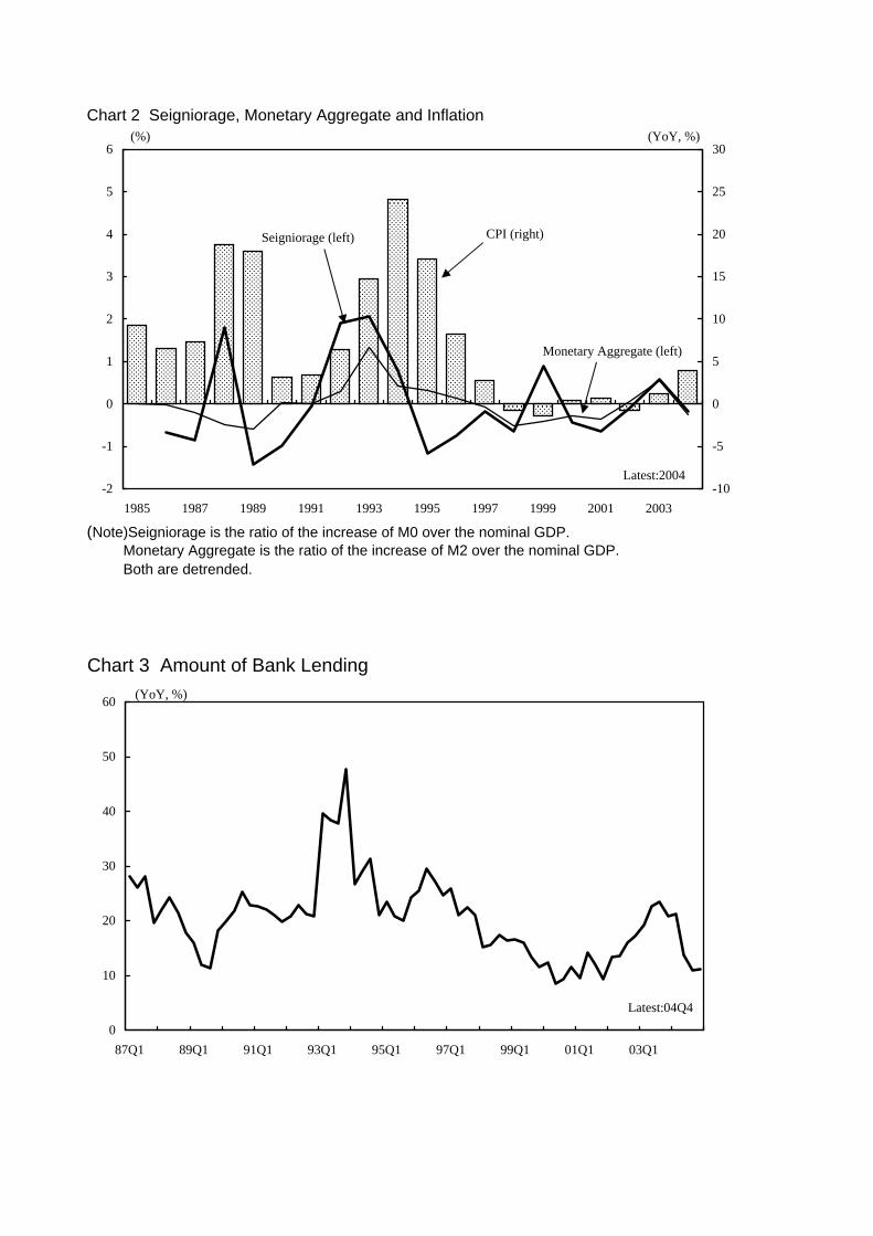
Chart 2 Seigniorage, Monetary Aggregate and Inflation

(Note)Seigniorage is the ratio of the increase of M0 over the nominal GDP. Monetary Aggregate is the ratio of the increase of M2 over the nominal GDP. Both are detrended.

Chart 3 Amount of Bank Lending

-2

-1

0

1

2

3

4

5

6

1985 1987 1989 1991 1993 1995 1997 1999 2001 2003-10

-5

0

5

10

15

20

25

30(YoY, %)(%)

CPI (right)Seigniorage (left)

Monetary Aggregate (left)

Latest:2004

0

10

20

30

40

50

60

87Q1 89Q1 91Q1 93Q1 95Q1 97Q1 99Q1 01Q1 03Q1

(YoY, %)

Latest:04Q4

Chart 4 Labor Productivity

(Note)Labor Productivity: the real GDP over the number of employment. Number of Employment: total wage payment over per capita wage.

Chart 5 Contribution Decomposition of the Year-on-Year Rate of CPI

<Closeup of ex. Food Contribution>

-0.10

-0.05

0.00

0.05

0.10

0.15

0.20

0.25

1970 1972 1974 1976 1978 1980 1982 1984 1986 1988 1990 1992 1994 1996 1998 2000 2002

(YoY, %)

Latest:2003

-5

0

5

10

15

20

25

30

94Q1 94Q4 95Q3 96Q2 97Q1 97Q4 98Q3 99Q2 00Q1 00Q4 01Q3 02Q2 03Q1 03Q4 04Q3

(Contribution to YoY, %)

Latest:04Q4Food

ex. Food

CPI

-2

0

2

4

6

8

10

12

94Q1 94Q4 95Q3 96Q2 97Q1 97Q4 98Q3 99Q2 00Q1 00Q4 01Q3 02Q2 03Q1 03Q4 04Q3

Latest:04Q4

(Contribution to YoY, %)

Clothes

Entertainment andEducation

MiscellaneousHousing

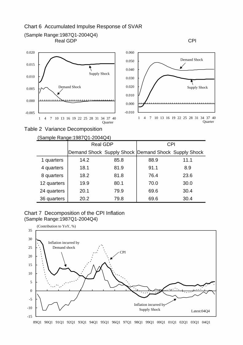
Chart 6 Accumulated Impulse Response of SVAR

(Sample Range:1987Q1-2004Q4) Real GDP CPI

Table 2 Variance Decomposition

(Sample Range:1987Q1-2004Q4)

Demand Shock Supply Shock Demand Shock Supply Shock

1 quarters 14.2 85.8 88.9 11.1

4 quarters 18.1 81.9 91.1 8.9

8 quarters 18.2 81.8 76.4 23.6

12 quarters 19.9 80.1 70.0 30.0

24 quarters 20.1 79.9 69.6 30.4

36 quarters 20.2 79.8 69.6 30.4

Chart 7 Decomposition of the CPI Inflation(Sample Range:1987Q1-2004Q4)

Real GDP CPI

-0.005

0.000

0.005

0.010

0.015

0.020

1 4 7 10 13 16 19 22 25 28 31 34 37 40

Supply Shock

Demand Shock

Quarter

-0.010

0.000

0.010

0.020

0.030

0.040

0.050

0.060

1 4 7 10 13 16 19 22 25 28 31 34 37 40

Supply Shock

Demand Shock

Quarter

-15

-10

-5

0

5

10

15

20

25

30

35

89Q1 90Q1 91Q1 92Q1 93Q1 94Q1 95Q1 96Q1 97Q1 98Q1 99Q1 00Q1 01Q1 02Q1 03Q1 04Q1

(Contribution to YoY, %)

Inflation incurred byDemand shock

Inflation incurred bySupply Shock

CPI

Latest:04Q4

Chart 8 Electricity Consumption per Unit of Capital

(Note)Electricity Consumption per Unit of Capital=Electricity Production over Capital Stock. Figure multiplied 100 is shown in the graph.

Chart 9 Two Output Gaps of Production Function Approarch

Table 3 Cross Correlation between Output Gap and Inflation (Annual Basis)

(Period:1970-2004)Leads to the Inflation -1 0 +1 +2 +3

Orthodox Output Gap 0.26 0.52 0.49 0.22 -0.01

Electricity Output Gap 0.30 0.57 0.64 0.45 0.08(Note)-1 means GDP Gap lags behind the inflation.

12

14

16

18

20

22

24

1970 1972 1974 1976 1978 1980 1982 1984 1986 1988 1990 1992 1994 1996 1998 2000 2002 2004

(Kwh)

-8

-4

0

4

8

12

16

1978 1980 1982 1984 1986 1988 1990 1992 1994 1996 1998 2000 2002 2004-15

-10

-5

0

5

10

15

20

25

30(YoY, %)(Natural Logarithm,×100)

CPI(right)Orthodox Output Gap

(left)

Electricity Output Gap(left)

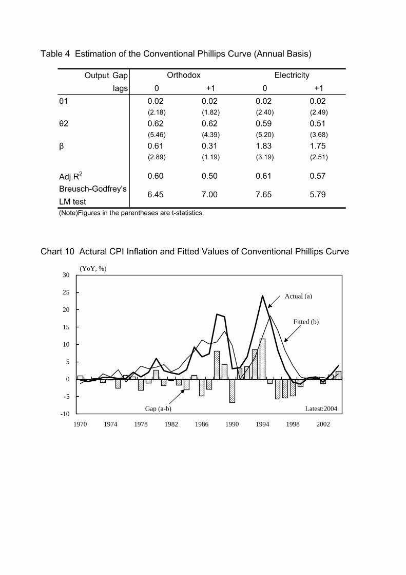
Table 4 Estimation of the Conventional Phillips Curve (Annual Basis)

Output Gaplags 0 +1 0 +1

θ1 0.02 0.02 0.02 0.02(2.18) (1.82) (2.40) (2.49)

θ2 0.62 0.62 0.59 0.51(5.46) (4.39) (5.20) (3.68)

β 0.61 0.31 1.83 1.75(2.89) (1.19) (3.19) (2.51)

Adj.R2 0.60 0.50 0.61 0.57Breusch-Godfrey'sLM test(Note)Figures in the parentheses are t-statistics.

Chart 10 Actural CPI Inflation and Fitted Values of Conventional Phillips Curve

Orthodox Electricity

6.45 7.00 7.65 5.79

-10

-5

0

5

10

15

20

25

30

1970 1974 1978 1982 1986 1990 1994 1998 2002

(YoY, %)

Latest:2004

Actual (a)

Fitted (b)

Gap (a-b)

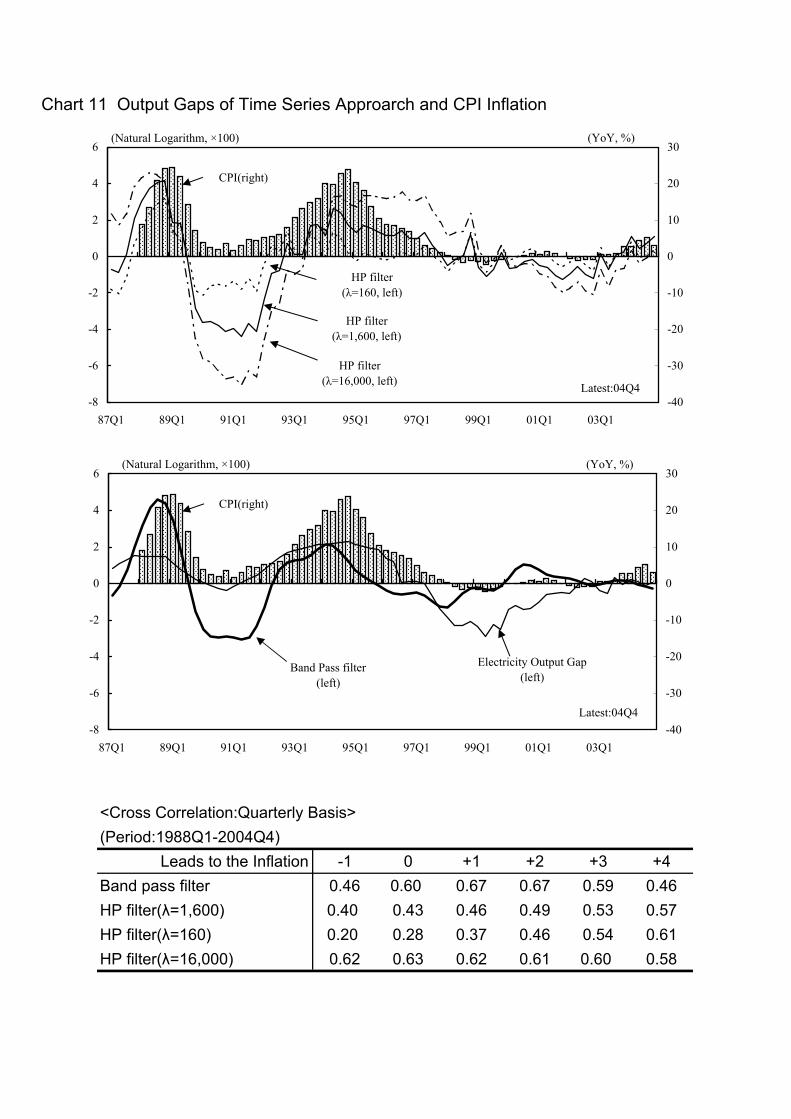
Chart 11 Output Gaps of Time Series Approarch and CPI Inflation

<Cross Correlation:Quarterly Basis>(Period:1988Q1-2004Q4)

Leads to the Inflation -1 0 +1 +2 +3 +4Band pass filter 0.46 0.60 0.67 0.67 0.59 0.46HP filter(λ=1,600) 0.40 0.43 0.46 0.49 0.53 0.57HP filter(λ=160) 0.20 0.28 0.37 0.46 0.54 0.61HP filter(λ=16,000) 0.62 0.63 0.62 0.61 0.60 0.58

-8

-6

-4

-2

0

2

4

6

87Q1 89Q1 91Q1 93Q1 95Q1 97Q1 99Q1 01Q1 03Q1-40

-30

-20

-10

0

10

20

30(YoY, %)

CPI(right)

HP filter(λ=1,600, left)

HP filter(λ=16,000, left)

HP filter(λ=160, left)

(Natural Logarithm, ×100)

Latest:04Q4

-8

-6

-4

-2

0

2

4

6

87Q1 89Q1 91Q1 93Q1 95Q1 97Q1 99Q1 01Q1 03Q1-40

-30

-20

-10

0

10

20

30(YoY, %)

CPI(right)

Band Pass filter(left)

Latest:04Q4

Electricity Output Gap(left)

(Natural Logarithm, ×100)

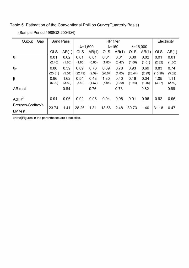
Table 5 Estimation of the Conventional Phillips Curve(Quarterly Basis)

(Sample Period:1988Q2-2004Q4)

(Note)Figures in the parentheses are t-statistics.

Output Gap

OLS AR(1) OLS AR(1) OLS AR(1) OLS AR(1) OLS AR(1)θ1 0.01 0.02 0.01 0.01 0.01 0.01 0.00 0.02 0.01 0.01

(2.40) (1.80) (1.85) (0.85) (1.83) (0.47) (1.06) (1.01) (2.32) (1.30)

θ2 0.86 0.59 0.89 0.73 0.89 0.78 0.93 0.69 0.83 0.74(25.81) (5.54) (22.49) (2.59) (26.07) (1.83) (23.44) (2.99) (15.98) (5.32)

β 0.96 1.62 0.54 0.43 1.30 0.40 0.16 0.34 1.05 1.11(6.00) (3.59) (3.43) (1.67) (5.04) (1.20) (1.64) (1.46) (3.37) (2.50)

AR root 0.84 0.76 0.73 0.82 0.69

Adj.R2 0.94 0.96 0.92 0.96 0.94 0.96 0.91 0.96 0.92 0.96Breusch-Godfrey'sLM test

Band Passλ=1,600 λ=160 λ=16,000

HP filter Electricity

23.74 1.41 28.26 1.81 31.18 0.4718.56 2.48 30.73 1.40

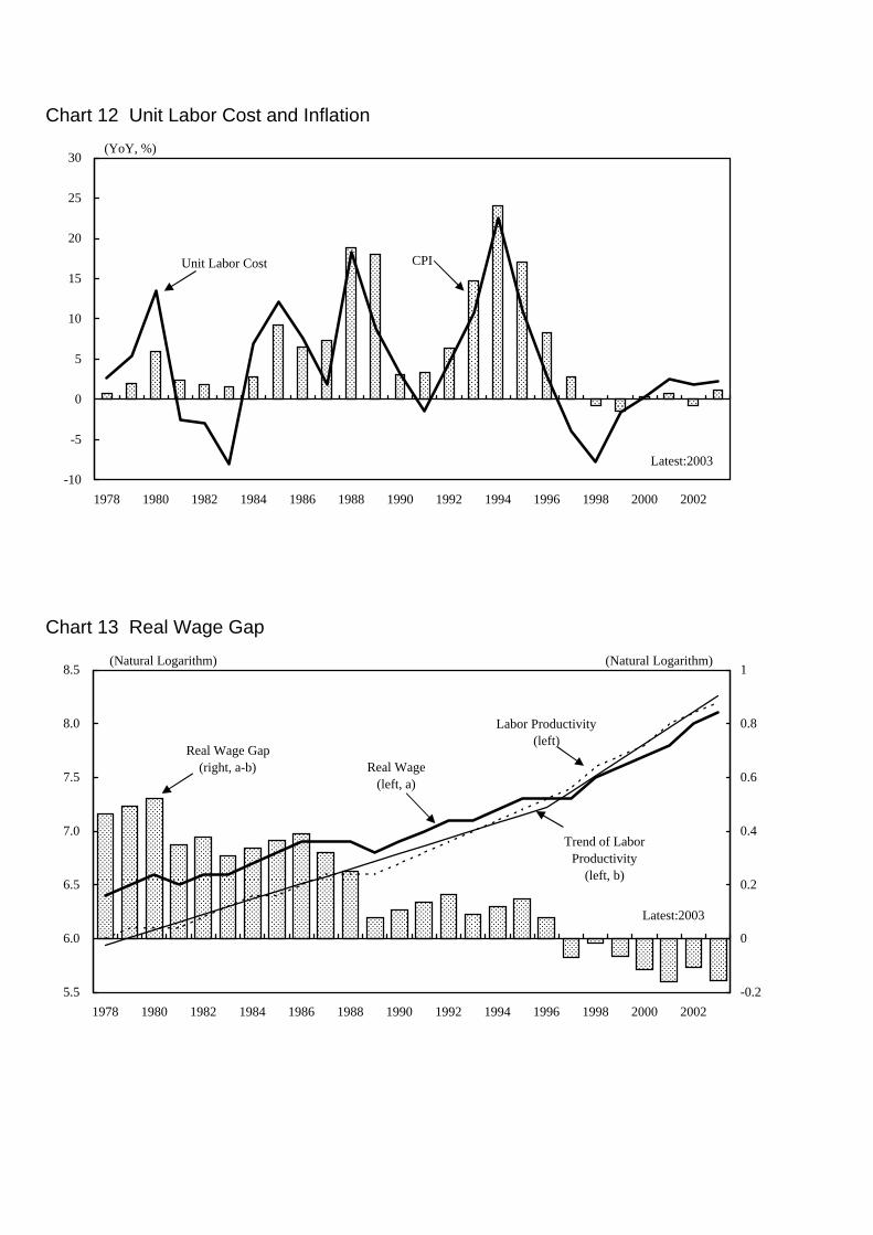
Chart 12 Unit Labor Cost and Inflation

Chart 13 Real Wage Gap

5.5

6.0

6.5

7.0

7.5

8.0

8.5

1978 1980 1982 1984 1986 1988 1990 1992 1994 1996 1998 2000 2002-0.2

0

0.2

0.4

0.6

0.8

1(Natural Logarithm)

Real Wage(left, a)

Trend of LaborProductivity

(left, b)

Real Wage Gap(right, a-b)

Latest:2003

Labor Productivity(left)

(Natural Logarithm)

-10

-5

0

5

10

15

20

25

30

1978 1980 1982 1984 1986 1988 1990 1992 1994 1996 1998 2000 2002

(YoY, %)

CPIUnit Labor Cost

Latest:2003

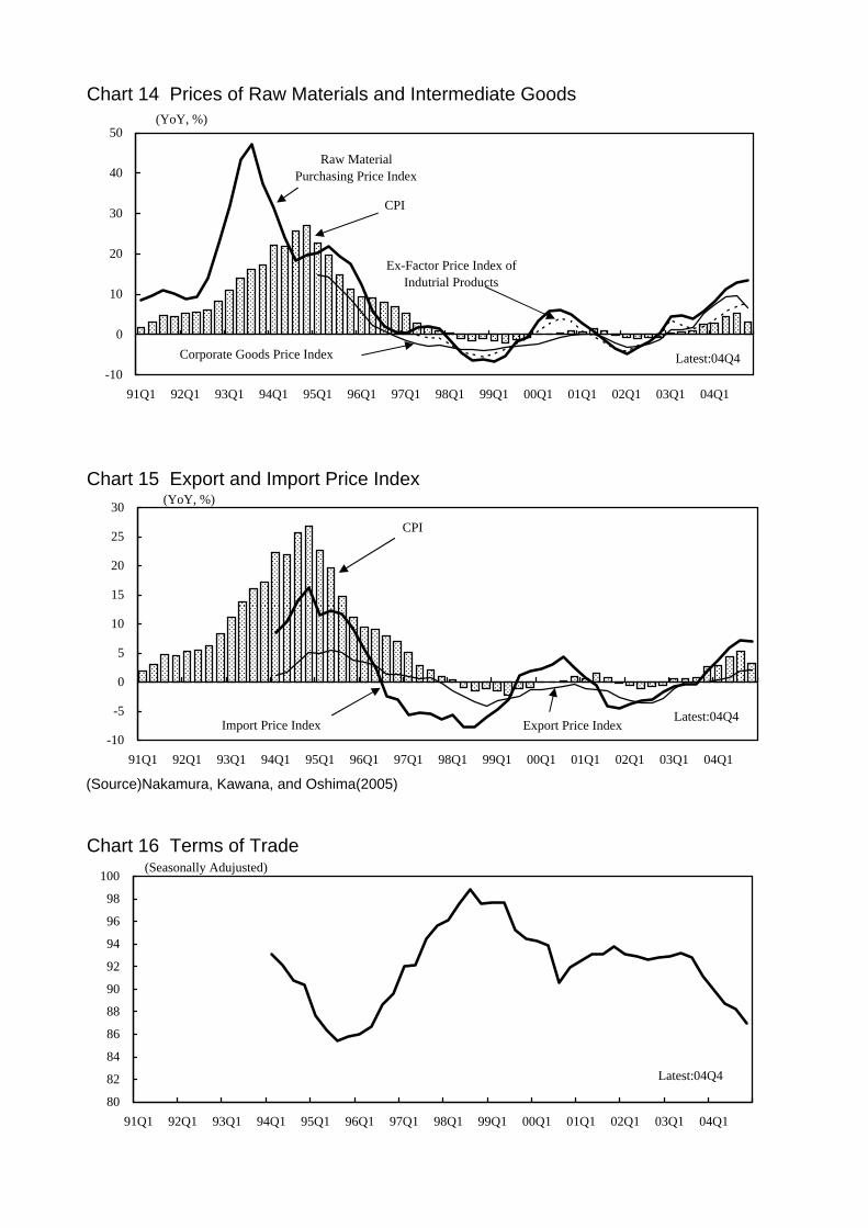
Chart 14 Prices of Raw Materials and Intermediate Goods

Chart 15 Export and Import Price Index

(Source)Nakamura, Kawana, and Oshima(2005)

Chart 16 Terms of Trade

-10

0

10

20

30

40

50

91Q1 92Q1 93Q1 94Q1 95Q1 96Q1 97Q1 98Q1 99Q1 00Q1 01Q1 02Q1 03Q1 04Q1

(YoY, %)

Raw MaterialPurchasing Price Index

Corporate Goods Price Index

Ex-Factor Price Index ofIndutrial Products

CPI

Latest:04Q4

-10

-5

0

5

10

15

20

25

30

91Q1 92Q1 93Q1 94Q1 95Q1 96Q1 97Q1 98Q1 99Q1 00Q1 01Q1 02Q1 03Q1 04Q1

Latest:04Q4Import Price Index Export Price Index

(YoY, %)

CPI

80

82

84

86

88

90

92

94

96

98

100

91Q1 92Q1 93Q1 94Q1 95Q1 96Q1 97Q1 98Q1 99Q1 00Q1 01Q1 02Q1 03Q1 04Q1

(Seasonally Adujusted)

Latest:04Q4

Table 6 Cross Correlation among Several Price Indeices

(Period:1997Q1-2004Q4)

Import PriceRaw MaterialPurchasing

Price

Ex-FactoryPrice of IP

CorporateGoods Price

ConsumerPrice

Import Price 1.00 -0.46 0.61 0.66 0.53(7) (0) (0) (0)

Raw Material 1.00 -0.36 -0.35 -0.33Purchasing Price (6) (1) (0)

Ex-Factory 1.00 0.43 0.51Price of IP (0) (3)

Corpotate 1.00 0.77Goods Price (0)

Consumer Price 1.00(Note)All series are seasonally adjusted by X-12-ARIMA. Cross Correlation is based on QoQ. Figures in the parentheses are the number of leads of column variables to raw variables.

Table 7 Unit Root Tests(Sample Period:1987Q1-2004Q4)

ADF PP DF-GLS KPSS ADF PP DF-GLS KPSSReal GDP -0.354 -3.07 0.826 1.133*** -2.979 -1.568 -2.818 0.512**

(0) (4) (4) (4)CPI -2.762* -2.661* -0.563 1.014*** -2.219 -0.905 -1.792 0.255***

(2) (2) (2) (2)M2 -3.039** -2.318 0.222 1.122*** 0.247 -0.186 -0.927 0.262***

(0) (3) (0) (3)(Note)*, **, *** mean the null hypothesis is rejected at the 10%, 5%, and 1% significant level, respectively. Figures in the parentheses are lag numbers.

Table 8 Cointegration Test

(Sample Period:1987Q1-2004Q4)

Table 9 Estimation of VECM(Sample Period:1988Q4-2004Q4)Long-run Equilibrium

VECM

Constant Constant & Linear Trend

Trace Max Eigenvalue

no 36.25 21.19cointegration (0.01) (0.05)

one 15.07 13.06cointegration (0.06) (0.08)

two 2.01 2.01cointegration (0.16) (0.16)

(Note) Figures in the parentheses are p-value. Shadow areas show the null hypothesis cannot be rejected at the 5% significant level.

Null H

ypothesis

y + 0.435*p - 0.544*m - 4.589 = 0(0.036) (0.012)

EC -0.216 *** -0.153 *** -0.454 *** (Note) Figures in the parentheses are the standard errors. *, **, *** mean the null hypothesis is rejected at the 10%, 5%, and 1% significant level, respectively.

Dependent Variable ∆y ∆p ∆m

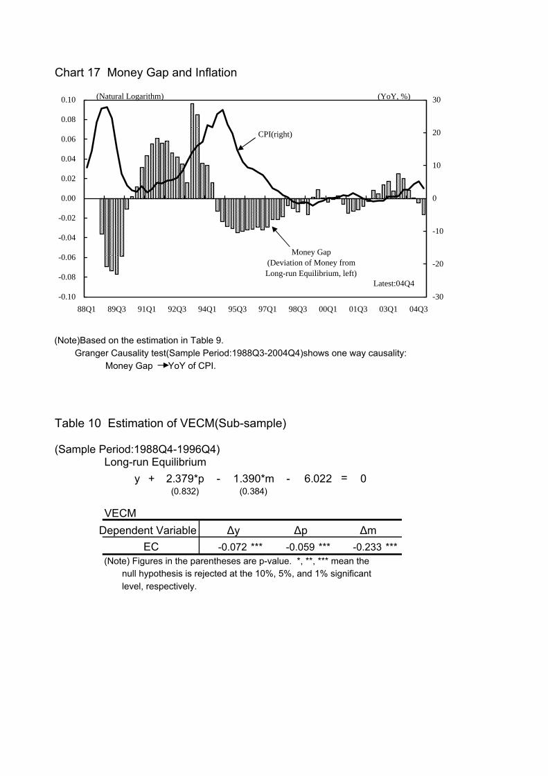
Chart 17 Money Gap and Inflation

(Note)Based on the estimation in Table 9. Granger Causality test(Sample Period:1988Q3-2004Q4)shows one way causality: Money Gap YoY of CPI.

Table 10 Estimation of VECM(Sub-sample)

(Sample Period:1988Q4-1996Q4)Long-run Equilibrium

VECMDependent Variable

EC -0.072 *** -0.059 *** -0.233 ***(Note) Figures in the parentheses are p-value. *, **, *** mean the null hypothesis is rejected at the 10%, 5%, and 1% significant level, respectively.

∆y ∆p ∆m

-0.10

-0.08

-0.06

-0.04

-0.02

0.00

0.02

0.04

0.06

0.08

0.10

88Q1 89Q3 91Q1 92Q3 94Q1 95Q3 97Q1 98Q3 00Q1 01Q3 03Q1 04Q3-30

-20

-10

0

10

20

30(YoY, %)

CPI(right)

Money Gap(Deviation of Money fromLong-run Equilibrium, left)

Latest:04Q4

(Natural Logarithm)

y + 2.379*p - 1.390*m - 6.022 = 0(0.832) (0.384)

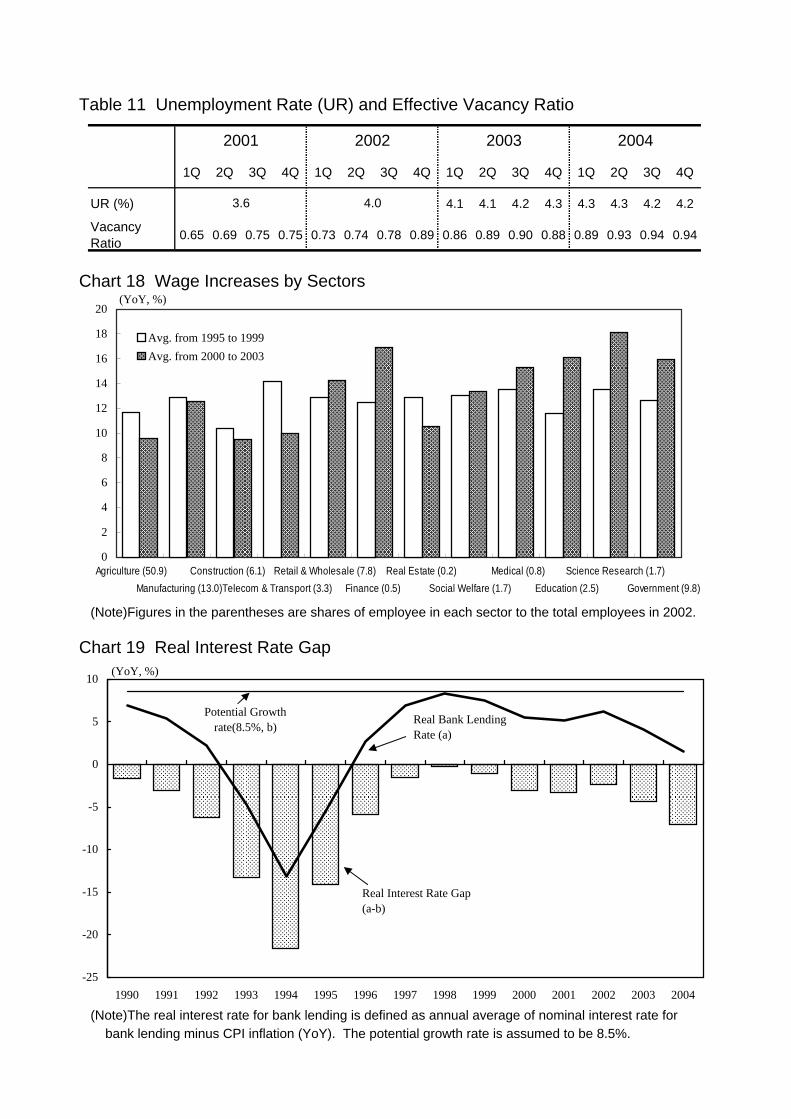
Table 11 Unemployment Rate (UR) and Effective Vacancy Ratio

1Q 2Q 3Q 4Q 1Q 2Q 3Q 4Q 1Q 2Q 3Q 4Q 1Q 2Q 3Q 4Q

UR (%) 4.1 4.1 4.2 4.3 4.3 4.3 4.2 4.2

VacancyRatio

0.65 0.69 0.75 0.75 0.73 0.74 0.78 0.89 0.86 0.89 0.90 0.88 0.89 0.93 0.94 0.94

Chart 18 Wage Increases by Sectors

(Note)Figures in the parentheses are shares of employee in each sector to the total employees in 2002.

Chart 19 Real Interest Rate Gap

(Note)The real interest rate for bank lending is defined as annual average of nominal interest rate for bank lending minus CPI inflation (YoY). The potential growth rate is assumed to be 8.5%.

2004

4.03.6

200320022001

-25

-20

-15

-10

-5

0

5

10

1990 1991 1992 1993 1994 1995 1996 1997 1998 1999 2000 2001 2002 2003 2004

(YoY, %)

Real Interest Rate Gap(a-b)

Real Bank LendingRate (a)

Potential Growthrate(8.5%, b)

0

2

4

6

8

10

12

14

16

18

20

Avg. from 1995 to 1999

Avg. from 2000 to 2003

(YoY, %)

Agriculture (50.9) Construction (6.1) Retail & Wholesale (7.8) Real Estate (0.2) Medical (0.8) Science Research (1.7)

Manufacturing (13.0) Telecom & Transport (3.3) Finance (0.5) Social Welfare (1.7) Education (2.5) Government (9.8)