Image and video processing - Centre national de la … Bonneel1 James Tompkin2 Kalyan Sunkavalli3...

Image and video processing(mostly via Poisson equation!)

Nicolas Bonneel

Poisson Image Editing

“Poisson Image Editing”, Perez et al. 2003

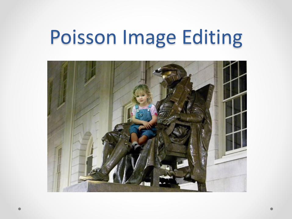
Poisson Image Editing• How it works ?

o The eye is more sensitive to color differences than absolute color values

o We thus try to preserve color differences: min 𝛻𝑢 − 𝛻𝑔 2𝑑𝑥

o This leads to the equation :

Δ𝑢 = Δg in Ω𝑢 = 𝑓 on 𝜕Ω

f g Ω





Δ(𝑢 − 𝑔) = 0 in Ω𝑢 − 𝑔 = 𝑓 − 𝑔 on 𝜕Ω

f g Ω𝑣





Δ𝑣 = 0 in Ω𝑣 = 𝑓 − 𝑔 on 𝜕Ω

f g Ω





4𝑣𝑥,𝑦 − 𝑣𝑥+1,𝑦 − 𝑣𝑥,𝑦+1 − 𝑣𝑥−1,𝑦 − 𝑣𝑥,𝑦−1 = 0 in Ω

𝑣𝑥,𝑦 = 𝑓𝑥,𝑦 − 𝑔𝑥,𝑦 on 𝜕Ω

f g Ω

𝑣𝑥,𝑦





𝑣𝑥,𝑦 =1

4(𝑣𝑥+1,𝑦 + 𝑣𝑥,𝑦+1 + 𝑣𝑥−1,𝑦 + 𝑣𝑥,𝑦−1) in Ω

𝑣𝑥,𝑦 = 𝑓𝑥,𝑦 − 𝑔𝑥,𝑦 on 𝜕Ωf g Ω

𝑣𝑥,𝑦





𝑣′𝑥,𝑦 =1

4(𝑣𝑥+1,𝑦 + 𝑣𝑥,𝑦+1 + 𝑣𝑥−1,𝑦 + 𝑣𝑥,𝑦−1) in Ω

𝑣′𝑥,𝑦 = 𝑓𝑥,𝑦 − 𝑔𝑥,𝑦 on 𝜕Ωf g Ω

𝑣′𝑥,𝑦





𝑣′𝑥,𝑦 = "𝑏𝑙𝑢𝑟" in Ω

𝑣′𝑥,𝑦 = 𝑓𝑥,𝑦 − 𝑔𝑥,𝑦 on 𝜕Ω

f g Ω

+ +

+

+

𝑣′𝑥,𝑦

Poisson Image Editing• Blur result :

__global__ void relax(float4 *out, int w, int h) {

int x = blockIdx.x*blockDim.x + threadIdx.x;

int y = blockIdx.y*blockDim.y + threadIdx.y;

if (x >= w || y >= h) { return; }

float4 mask_up = tex2D(mask, x, y-1), ;

float4 mask_dwn = tex2D(mask, x, y+1);

float4 mask_left = tex2D(mask x-1, y);

float4 mask_rght = tex2D(mask, x+1, y);

float4 baby_up = tex2D(baby, x, y-1);

float4 baby_dwn = tex2D(baby, x, y+1);

float4 baby_left = tex2D(baby, x-1, y);

float4 baby_rght = tex2D(baby, x+1, y);

float4 u_up = (tex2D(statue, x, y-1) - baby_up) * (1.- mask_up) + tex2D(prev_iter, x, y-1) * mask_up;

float4 u_dwn = (tex2D(statue, x, y+1)- baby_dwn) * (1.- mask_dwn) + tex2D(prev_iter, x, y+1) * mask_dwn;

float4 u_left = (tex2D(statue, x-1, y) - baby_left) * (1.- mask_left) + tex2D(prev_iter, x-1, y) * mask_left;

float4 u_rght = (tex2D(statue, x+1, y) - baby_rght) * (1.- mask_rght) + tex2D(prev_iter, x+1, y) * mask_rght;

float4 val = (u_up + u_dwn + u_left + u_rght)/4.;

float4 mask_center = tex2D(mask, x, y);

out[y * w + x] = val*mask_center + (1,-mask_center)*tex2D(statue, x, y);

}



o We thus try to preserve color differences

o Once 𝑣 is known, 𝑢 = 𝑔 + 𝑣

Quality highly depends on boundary (→ boundary optimization techniques)

f g Ω

+ +

+

+

𝑣′𝑥,𝑦

Poisson Image Editing• Problem : Slow to converge + numerical precision issues

• Solution : Multigrid

Extended to meshes

“Mesh Editing with Poisson-Based Gradient Field Manipulation”, Yu et al. 2004

Generalizations• L1 reconstruction

o Use min 𝛻𝑢 − 𝛻𝑔 1𝑑𝑥 instead of min 𝛻𝑢 − 𝛻𝑔 2𝑑𝑥

o Yields local formulation: div𝛻𝑢−𝛻𝑔

|𝛻𝑢−𝛻𝑔|= 0

o More complex to minimize (nonlinear)

• Adding a spatial weighting termo min 𝑤 𝑥 𝛻𝑢 − 𝛻𝑔 2𝑑𝑥

o Yields local formulation: div 𝑤 𝑥 𝛻𝑢 − 𝛻g = 0

• General form:o min 𝑤(|𝛻𝑢 − 𝛻𝑔|)𝑑𝑥

o Yields local formulation: div𝑤′ 𝛻𝑢−𝛻𝑔

𝛻𝑢−𝛻𝑔𝛻𝑢 − 𝛻𝑔 = 0

o Most often non linear ; recovers linear isotropic diffusion with 𝑤 𝑢 = 𝑢2

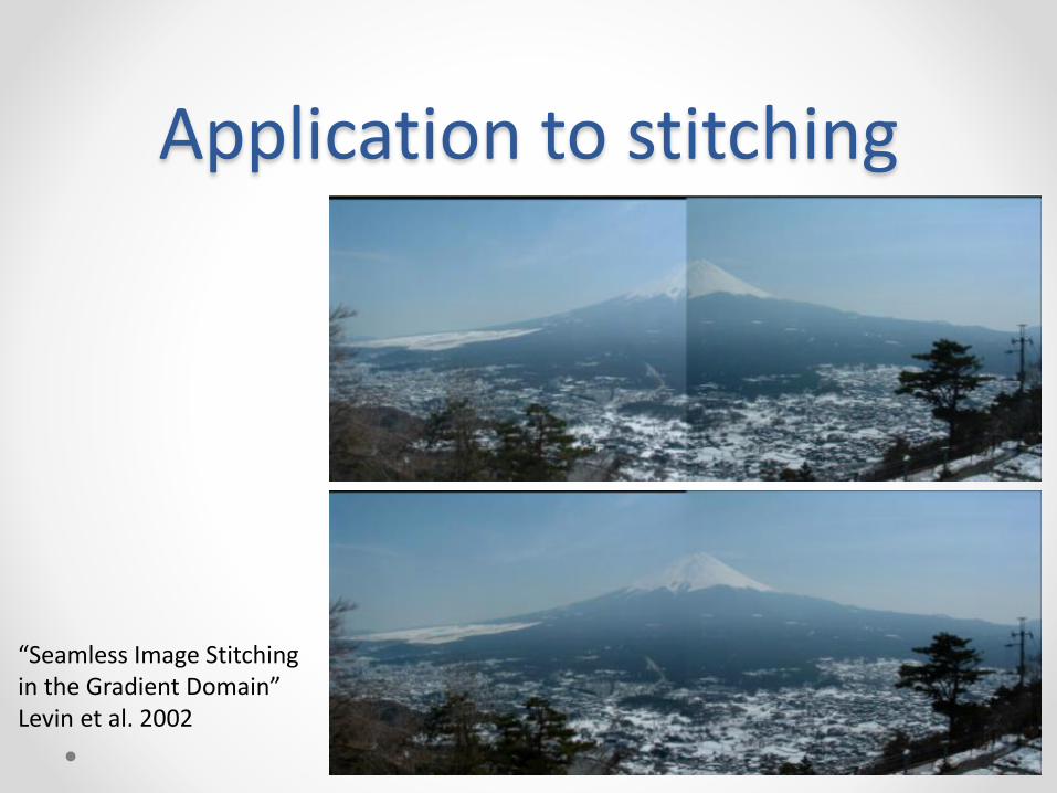
Application to stitching

“Seamless Image Stitching in the Gradient Domain”Levin et al. 2002

Intrinsic decompositions

“User-Assisted Intrinsic Images”, Bousseau et al. 2009

Intrinsic decompositions𝐼 = 𝑆. 𝑅

Image Shading Reflectance

• The Retinex assumption:o Shading layer smoother than reflectance layer

o So, shading gradients are smaller

o Color Retinex: if a gradient is colored, most likely comes from reflectance

• Ideas:o Work in log-domain : log 𝐼 = log 𝑆 + log𝑅

o Work with gradients : 𝛻 log 𝐼 = 𝛻 log 𝑆 + 𝛻 log𝑅

o Now, identify gradients belonging to either (log) S or R

“Ground truth dataset and baseline evaluations for intrinsic image algorithms”, Grosse et al. 09

Intrinsic decompositions• Denote 𝑟𝑥 the horizontal gradient of log 𝑅 (same for 𝑦, I

and S)

• Color Retinex algorithm:o If 𝑖𝑥

𝑏𝑟 > 𝑇𝑏𝑟 𝑎𝑛𝑑 𝑖𝑥𝑐ℎ𝑟 > 𝑇𝑐ℎ𝑟, 𝑟𝑥 = 𝑖𝑥

𝑏𝑟 𝑒𝑙𝑠𝑒 𝑟𝑥 = 0

o Reconstruct R by solving a Poisson equation Δ log 𝑅 = Δ𝑟

• Can alternatively use an L1 reconstruction min 𝛻 log 𝑅 − 𝛻𝑟 𝑑𝑥

o Obtain shading: 𝑆 = 𝐼/𝑅

Intrinsic decompositions• Extensions:

o Add non-local constraints on reflectance

o Constrain reflectance colors to be sparse

o Add reflectance constraints in time (for videos)

o Add user constraints

• Applications:o Re-texturing ; re-lighting

o Image compositing

o Better optical flows

o Image segmentation

o Scene understanding...

Intrinsic decompositions• Other approaches:

o Based on machine learning: Neural networks, Conditional Random Fields ...

• Difficulty: finding ground truth decompositions to learn from

o Approaches estimating jointly shape, environment map and intrinsic decomposition

o Algorithms based on other assumptions

• Line model: Under skylight, pixels of same reflectance on same log-RGB line

• Locally linear reflectance model

Intrinsic decomposition• Ground truth images

o Realistic scenes difficult to obtain

o No good definition for specular scenes

Blind Video Temporal Consistency

1CNRS / LIRIS3Adobe Research

2

Nicolas Bonneel1 James Tompkin2 Kalyan Sunkavalli3

Deqing Sun2 Sylvain Paris3 Hanspeter Pfister2

26

Observation

Image processing algorithms are often temporally unstable

HDR Tone Mapping Spatial White Balance Intrinsic Decomposition

27

Observation

Image processing algorithms are often temporally unstable

HDR Tone Mapping Spatial White Balance Intrinsic Decomposition

28

each frame processed independently

GoalInput video

=

29

Image processing per frame

+

Stable video processing(our result)

Method

30[Bonneel et al. - Blind Video

Temporal Consistency]

Variational formulation

min 𝛻𝑂𝑛 − 𝛻𝑃𝑛2

High frequency scene dynamics

31

Input video (V) Processed video (P) Output video (O)


min 𝛻𝑂𝑛 − 𝛻𝑃𝑛2 + 𝑂𝑛 −𝑤𝑎𝑟𝑝 𝑂𝑛−1

2


Temporal consistency

32



min 𝛻𝑂𝑛 − 𝛻𝑃𝑛2 +𝑤 𝑥 𝑂𝑛 −𝑤𝑎𝑟𝑝 𝑂𝑛−1

2


Temporal consistency

𝑤 = λ exp(− 𝑉𝑛 − 𝑤𝑎𝑟𝑝 𝑉𝑛−1 )

33


• Temporal consistency strengtho Scalar factor λ in w(x)

• “warp” operatoro Optical flow methods

[Sun et al. 2014] or [Wulff and Black 2015]

o Nearest neighbor fields[PatchMatch, Barnes et al. 2009]

User parameters

34

min 𝛻𝑂𝑛 − 𝛻𝑃𝑛2 + 𝑤 𝑥 𝑂𝑛 − 𝑤𝑎𝑟𝑝 𝑂𝑛−1

2

Screened Poisson Equation

• Energy can be minimized locally

−Δ𝑂𝑛 +𝑤 𝑥 𝑂𝑛 = −Δ𝑃𝑛 +𝑤 𝑥 𝑤𝑎𝑟𝑝 𝑂𝑛−1

• Standard linear equationo Details in the paper

35


Fourier analysis (const. w)

ℱ 𝑂𝑛 𝜉 = 1 − 𝛼 ℱ 𝑃𝑛 + 𝛼 ℱ(𝑤𝑎𝑟𝑝 𝑂𝑛−1 )

with 𝛼 =𝑤

4𝜋2𝜉2+𝑤depends on spatial frequency 𝜉

• Low and high spatial frequencies treated differentlyo Low frequencies more regularized

o Unlike previous work that treats them uniformly



Processed(current frame)

Output (previous frame)

Output(current frame)

Synthetic test

High frequencynoise

(except first frame)

Our result(not suitable for

denoising)

37

Synthetic test

Low frequency noise

(except first frame)

Our result

38

Results

39

Color grading

Input video Per-frame processing

40

Color grading

Our result

41

Spatial White Balance [Hsu et al. 2008]


42

Input video Our result

43

Spatial White Balance [Hsu et al. 2008]

Intrinsic Images [Bell et al. 2014]


44

Intrinsic Images [Bell et al. 2014]


45

Dehazing[Tang et al. 2014]

46


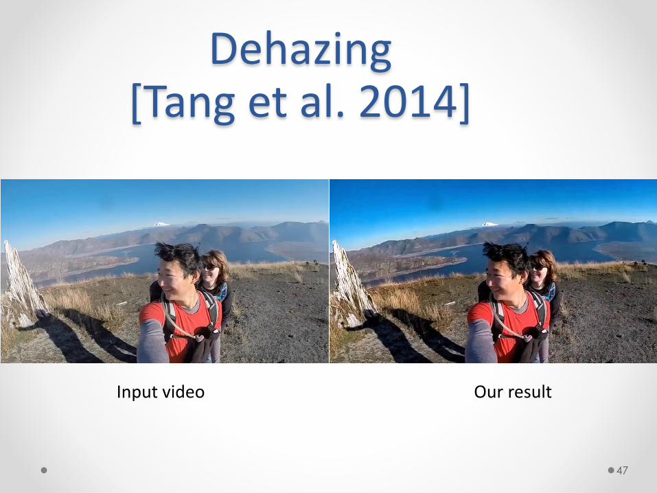
Dehazing[Tang et al. 2014]

47


Limitations

Processing creating edges Matting



Conclusion

• “Blind” approach to temporal consistencyo Supported by Fourier analysis

• Wide range of image processing ported to videoso Can be applied as is to current and future algorithms

• C++ code http://liris.cnrs.fr/~nbonneel/consistency/



“Remove occupant…”Texture synthesis

(also works with ex-gf/bf)

“Parallel Controllable Texture Synthesis”, Lefebvre and Hoppe 2005

Texture synthesis• Idea : copy pixels from the image that are coherent with an

initial guess


initial guess

Initial guess


initial guess

Refinement

Texture synthesis• Multi-resolution && initialization

Initialization here

Texture synthesis• ok – but artifacts

Texture synthesis• Idea : use a guide

“Image Analogies”, Hertzmann et al. 2001 (image-by-number approach)

Texture synthesis• Idea : use a guide

Texture synthesis• Extension:

o copy pixel gradients instead of pixels

o Reconstruct an image with Poisson equation

Proxy-Guided Texture Synthesis

“Proxy-Guided Texture Synthesis for Rendering Natural Scenes”, Bonneel et al. 2010

Texture synthesis• That’s the dinosaur version of Neural style transfer:

“A Neural Algorithm of Artistic Style”, Gatys et al. 2015

Gradient Shop• Demoes filters achievable in the gradient domain

• Keeps a screened Poisson formulation∇. 𝑤 𝑥 ∇𝑢 − 𝐹 ∇𝐼 + 𝑤′ 𝑥 𝑢 − 𝐺 𝐼 = 0

o Sharpening: 𝐹 𝛻𝐼 = 𝑐. ∇𝐼 𝐺 𝐼 = 𝐼 𝑤 = 1 𝑤′ = 𝑑

• More robust with spatially varying w

o NPR: 𝐹𝑥 ∇𝐼 = cos2 𝑒 .𝜕𝐼

𝜕𝑥𝑛 𝐹𝑦 𝛻𝐼 = sin2 𝑒 .

𝜕𝐼

𝜕𝑦𝑛

𝐺 𝐼 = 𝐼 𝑤′ = 𝑑

With e an edge detector, and n another weighting term

o etc. etc.

“GradientShop: A Gradient-Domain Optimization Framework for Image and Video Filtering”, Bhat et al. 2008

Depth of Field• Circle of confusion: 𝑐 =

𝐹2

𝑛 (𝑍𝑓−𝐹)

𝑍−𝑍𝑓

𝑍= 𝛼

𝑍−𝑍𝑓

𝑍

o Z: depth ; 𝑍𝑓: focal distance ; F: focal length ; 𝑛: aperture

• Consider anisotropic diffusion:

o𝜕𝐼

𝜕𝑡= ∇. (𝑔 ∇𝐼) where 𝑔 is the diffusivity

o Take 𝑔 = 𝛼𝑍−𝑍𝑓

2

𝑍2

“Real-time, Accurate Depth of Field using Anisotropic Diffusion and Programmable Graphics Cards”, Bertalmio et al. 2004

Diffusion curves

• Two Poisson equations:o Δ𝐼 = 𝑑𝑖𝑣 𝑤 for colors (+ user constraints to I)

o Δ𝐵 = 0 for blur (+ 𝐵 = 𝜎 on curve)

• Then blur I using B with anisotropic diffusion

“Diffusion Curves: A Vector Representation for Smooth-Shaded Images”, Orzan et al. 2008

In rendering

Poisson in Rendering• Image derivatives of Metropolis light transport

o Augment path space with vertical and horizontal image offsets

o Estimate 𝐼𝑗+1 = ℎ𝑗+1 𝑥 𝑓 𝑥 𝑑𝜇(𝑥)

• 𝑥 in path space

• ℎ image filter

• 𝑓 image contribution

o Use both 𝐼𝑗+1 − 𝐼𝑗 (gradient) and 𝐼𝑗 (actual value)

o Drive sampler with a linear combination of both gradient norm and value

o Solve the Screened Poisson equation (L1 works better)

“Gradient-Domain Metropolis Light Transport”, Lehtinen et al. 2013

Poisson in Rendering

Poisson in Rendering• Simpler formulation with path tracing:

“Gradient-Domain Path Tracing”, Kettunen et al. 2015 – reading list.

Solvers

Solving the Poisson Equation• The Poisson equation Δ𝑢 = 𝑓 can be discretized in 2d:

o 4𝑣𝑥,𝑦 − 𝑣𝑥+1,𝑦 − 𝑣𝑥,𝑦+1 − 𝑣𝑥−1,𝑦 − 𝑣𝑥,𝑦−1 = fx,y (2nd order centered laplacian)

o In matrix form : 𝑀 𝑣 = 𝑓 with

𝑀 =

⋱−1 … −1 4 −1 … −1

−1 … −1 4 −1 …−1 … −1 4 −1

−1 … −1 4

• We have seen one method so faro 𝑣′𝑥,𝑦 =

1

4𝑣𝑥+1,𝑦 + 𝑣𝑥,𝑦+1 + 𝑣𝑥−1,𝑦 + 𝑣𝑥,𝑦−1 + f𝑥,𝑦

o This is the Jacobi method: 𝑀 = 𝐷 − 𝐿 − 𝑈 with 𝐷 = 𝑑𝑖𝑎𝑔(𝑀)

o 𝑀 𝑣 = 𝑓 ⇔ 𝐷 − 𝐿 − 𝑈 𝑣 = 𝑓 ⇔ 𝐷𝑣 = 𝐿 + 𝑈 𝑣 + 𝑓

o Build a converging sequence 𝐷𝑣(𝑘+1) = 𝐿 + 𝑈 𝑣(𝑘) + 𝑓

(in practice, this is –Laplacian)

Note: The solvers we’ll see here also apply to other linear systems like the Radiosity linear system we saw in week 2.

Solving the Poisson Equation• Jacobi is easy to parallelize but

o Converges iif 𝐷−1(𝐿 + 𝑈) has max abs. eigenvalue < 1

• Gershgorin argument just not enough here

• Depends on BC (e.g., periodic BC has max eig = 1)

o Converges if strictly diagonal dominant : not the case here

o In practice, converges super slowly (or even not at all due to numerical precision)

• Gauss-Seidel:o Instead: 𝐷 − 𝐿 − 𝑈 𝑣 = 𝑓 ⇔ 𝐷 − 𝐿 𝑣 = 𝑈𝑣 + 𝑓

o This corresponds to solving a triangular system via backsubstitution:

o 𝑣𝑖𝑘+1

=1

𝑀𝑖𝑖𝑓𝑖 − 𝑗=1

𝑖−1𝑀𝑖𝑗𝑣𝑗𝑘+1

− 𝑗=𝑖+1𝑛 𝑀𝑖𝑗𝑣𝑗

𝑘

o For Poisson : 𝑣′𝑥,𝑦 =1

4𝑣𝑥+1,𝑦 + 𝑣𝑥,𝑦+1 + 𝑣′𝑥−1,𝑦 + 𝑣′𝑥,𝑦−1 + f𝑥,𝑦

Solving the Poisson Equation• Gauss-Seidel:

o Converges faster

o Converges if SPD matrix

• Not necessarily: also depends on BC (in many cases, one degree of freedom) ; fixing them (Dirichlet) makes it ok

• for the case of Radiosity, granted by energy conservation and reciprocity

o Converges if strictly diagonal dominant

• Still nope

o In practice, converges a bit faster

o Not parallelizable (easily) : depends on previously solved values

Solving the Poisson Equation• Successive Over-Relaxation (SOR)

o Use a weighted combination of previous and current iteration with Gauss-Seidel

o 𝐷 − 𝐿 − 𝑈 𝑣 = 𝑓 ⇔ 𝜔 𝐷 − 𝐿 𝑣 = 𝜔𝑈𝑣 + 𝜔𝑓⇔ 𝐷 − 𝜔𝐿 𝑣 = 1 − 𝜔 𝐷 + 𝜔𝑈 + 𝜔𝑓

o Leads to 𝑣𝑖(𝑘+1)

= 1 − 𝜔 𝑣𝑖𝑘+

𝜔

𝑀𝑖𝑖𝑓𝑖 − 𝑗=1

𝑖−1𝑀𝑖𝑗𝑣𝑗𝑘+1

− 𝑗=𝑖+1𝑛 𝑀𝑖𝑗𝑣𝑗

𝑘

o For Poisson : 𝑣′𝑥,𝑦 = 1 − 𝜔 𝑣𝑥,𝑦 +𝜔

4𝑣𝑥+1,𝑦 + 𝑣𝑥,𝑦+1 + 𝑣′𝑥−1,𝑦 + 𝑣′𝑥,𝑦−1 + f𝑥,𝑦

• Convergenceo If SPD matrix, converges for 0 < 𝜔 < 2

o Expect to converge fast with 𝜔 > 1 (goes further than GS)

o For tridiagonal matrices (e.g., 1D Poisson): 𝜔𝑜𝑝𝑡 =2

1+ 1−𝜌( 𝐷−𝐿 −1𝑈)

o For 2D Poisson on an 𝑛 × 𝑛 grid: 𝜔𝑜𝑝𝑡 =2

1+sin(𝜋

𝑛)

Solving the Poisson Equation• Geometric Multigrid

o Last time we saw a multiscale approach. Good if we can build the rhs at any scale (e.g., Poisson Image Editing).

o Otherwise:

• Approximately solve 𝑀ℎ𝑣ℎ = 𝑓ℎ• Take residual 𝑟ℎ = 𝑓ℎ −𝑀ℎ𝑣ℎ and downsample it to 𝑟2ℎ• Approximately solve 𝑀2ℎ𝑟′2ℎ = 𝑟2ℎ• ... continue...

• Upsample 𝑟2ℎ′ to 𝑟ℎ

′ by interpolation

• Continue solving 𝑀ℎ𝑣′ℎ = 𝑓ℎ with 𝑣ℎ + 𝑟ℎ′ as starting point

o Converges *much* faster: solves a linear system in 𝑂(𝑛)

o Still requires the matrix 𝑀ℎ at any scale ℎ

• If not, see “Algebraic multigrid”

Solving the Poisson Equation• Conjugate Gradient

o Example: 𝑣 𝑘+1 = 𝑣(𝑘) + 𝑓 +𝑀𝑣(𝑘) (gradient descent for F 𝑣 =1

2𝑣𝑇𝑀𝑣 − 𝑓𝑣)

• Take 𝑣(1) = 𝑓

• Shows 𝑣(𝑘) in 𝒦𝑘 = 𝑆𝑝𝑎𝑛(𝑓,𝑀𝑓,𝑀2𝑓,… ,𝑀𝑘−1𝑓) : Krylov subspace

• Can build orthogonal basis for 𝒦𝑘 with Gram-Schmidt

o We want residual r k = 𝑓 −𝑀𝑣(𝑘) (which is in 𝒦𝑘+1) to be orthogonal to 𝒦𝑘

• Squeezes the residual to smaller and smaller subspaces

• So, r k orthogonal to 𝑟(𝑙) ∀𝑙 < 𝑘

o r k ⊥ 𝒦𝑘 and r k−1 ⊥ 𝒦𝑘−1 so r k − 𝑟(𝑘−1) ⊥ 𝒦𝑘−1

o and 𝑣(𝑙) − 𝑣 𝑙−1 ∈ 𝒦𝑘

o So: 𝑣 𝑙 − 𝑣 𝑙−1 𝑇r k − 𝑟 𝑘−1 = 0 for 𝑙 < 𝑘

o We have r k − r k−1 = −𝑀 𝑣 𝑘 − 𝑣 𝑘−1

o So: 𝑣 𝑙 − 𝑣 𝑙−1 𝑇𝑀 𝑣 𝑘 − 𝑣 𝑘−1 = 0 for 𝑙 < 𝑘

• The difference between iterates is M-conjugate

Solving the Poisson Equation• Conjugate Gradient

o 𝛼(𝑘) =𝑟 𝑘−1 𝑇 𝑟 𝑘−1

𝑑 𝑘−1 𝑇𝑀 𝑑 𝑘−1 // such that 𝑟 𝑘 ⊥ 𝑟 𝑘−1

o 𝑣 𝑘 = 𝑣 𝑘−1 + 𝛼 𝑘 𝑑 𝑘−1

o 𝑟 𝑘 = 𝑟 𝑘−1 − 𝛼 𝑘 𝑀𝑑 𝑘−1 // r k − r k−1 = −𝑀 𝑣 𝑘 − 𝑣 𝑘−1

o 𝛽 𝑘 =𝑟 𝑘 𝑇 𝑟 𝑘

𝑟 𝑘−1 𝑇 𝑟 𝑘−1 // such that 𝑑 𝑘 conjugate with 𝑑 𝑘−1

o 𝑑 𝑘 = 𝑟 𝑘 + 𝛽 𝑘 𝑑 𝑘−1

• Works for SPD matrices o Again, beware of BC for Poisson problems

• Convergence: 𝑥 − 𝑥𝑘 𝑀 ≤ 2𝜆𝑚𝑎𝑥− 𝜆𝑚𝑖𝑛

𝜆𝑚𝑎𝑥+ 𝜆𝑚𝑖𝑛

𝑘

𝑥 − 𝑥0 𝑀

Solving the Poisson Equation• These methods don’t require building the matrix M

o Only need applying matrix M to vector v

o That’s fortunate: even if matrices are sparse, direct solver can eat much memory

• In many cases (not Poisson), need preconditionerso Solver converge better when eigenvalues not too spread

o Instead solve : 𝑃 𝑀𝑣 = 𝑃𝑓 with 𝑃 ≈ 𝑀−1

• Jacobi preconditioner: 𝑃 = 𝑑𝑖𝑎𝑔 𝑀 −1

• ICP: Incomplete Cholesky (e.g., a band of Cholesky)

• Or any iterations we’ve seen so far (e.g., solve with CG, use multigrid preconditioner)

Solving the Poisson Equation• Fourier-based approach

o Δ𝑣 = 𝑓 ⟺ ℱ Δ𝑣 = ℱ 𝑓⟺ 4𝜋2|𝜉|2ℱ 𝑣 = ℱ 𝑓

o Numerically:

• When periodic BC, use FFT (and then inverse FFT) : 𝑣 =ℎ2 𝑓

2 cos𝜋𝑚

𝑀+ cos

𝜋𝑛

𝑁−2

• When Dirichlet BC ( 𝑣 = 0 ), use DST : 𝑣 =ℎ2 𝑓

2 cos𝜋𝑚

𝑀+cos

𝜋𝑛

𝑁−2

• When Neumann BC (∇𝑣 = 0), use DCT : 𝑣 =ℎ2 𝑓

2 cos𝜋𝑚

𝑀+cos

𝜋𝑛

𝑁−2

Solving the Poisson Equation• Green’s kernel approach

o Given solution of Δ𝐺 = 𝛿 with 𝐺 = 0 on 𝜕Ω,

• Solution of Δ𝑣 = 0 with 𝑣 = 0 on 𝜕Ω is 𝑣 = 𝐺 ∗ 𝑓

• Proof: Δ𝑣 = Δ 𝐺 ∗ 𝑓 = Δ𝐺 ∗ 𝑓 = 𝛿 ∗ 𝑓 = 𝑓

o Green’s kernel for Δ (in 2D) : 𝐺 𝜌 =1

2𝜋ln 𝜌

o Green’s kernel for 2d diffusion: 𝜕

𝜕𝑡− 𝑘Δ : 𝐺 𝑡, 𝜌 = 𝐻 𝑡

1

4𝜋 k texp −

𝜌2

4 𝑘 𝑡

• Gaussian convolutions

Application• Geodesic computation

o Varadhan’s formula: 𝑑 𝑥, 𝑦 = lim𝑡→0 −4𝑡 log 𝑘𝑡,𝑥 𝑦

• 𝑘𝑡,𝑥(𝑦) heat kernel: heat transferred from 𝑥 to 𝑦 after time 𝑡

• Too sensitive to errors

o We know that ∇𝑑 = 1 (Eikonal equation)

o Instead only consider ∇𝑣 of correct direction

• 𝑣 − 𝑡 Δ𝑣 = 0 on 𝑀 \ 𝛾

• 𝑣 0, 𝑥 = 1 on 𝛾

• Take just one Euler step to obtain 𝑣(𝜖, 𝑥)

• Consider vector field 𝑋 =∇𝑣

∇𝑣

• Solve Poisson eq. Δ𝑑 = ∇. 𝑋

“Geodesics in Heat: A New Approach to Computing Distance Based on Heat Flow”, [Crane et al. 2013]

Application• Discretization of Δ on meshes – see with Julie next time

• Solver:o Iterative ?

o Advocate for Cholesky factorization: eats memory and slow but can be reused

• Only depends on mesh (no BC!)

• Gives Δ = 𝐿𝐿𝑇 , solved via backsubstitution

Poisson Equation for Fluid simulation

The Navier-Stokes equations𝜕𝑢

𝜕𝑡+ 𝑢. ∇𝑢 +

1

𝜌∇p = g + 𝜈Δ𝑢

∇. 𝑢 = 0

𝐷𝑢

𝐷𝑡

(e.g., consider𝑑

𝑑𝑡𝑓 𝑥 𝑡 , 𝑡 and use chain rule)

~ acceleration

𝑚 𝑣 = 𝑓𝑜𝑟𝑐𝑒𝑠Forces: ∇𝑝 , 𝜌 𝑔, 𝜌𝜈Δ𝑢

Viscosity: deviation of 𝑢from average

“Fluid Simulation for Computer Graphics”, Bridson 2008 (book)

Incompressibility

Simple Fluid Solver• First 𝑢′ = advect 𝑢 + Δ𝑡 𝑔 based on interpolation

• Then 𝑢′′ = 𝑝𝑟𝑜𝑗𝑒𝑐𝑡 𝑢′

o 𝑢′′ = 𝑢′ − Δ𝑡1

𝜌∇𝑝

o Find 𝑝 such that 𝑢′′ incompressible: ∇. 𝑢′′ = ∇. 𝑢′ −Δ𝑡

𝜌Δ𝑝 = 0

o i.e., solve the Poisson equation Δ𝑝 =𝜌

Δ𝑡∇. 𝑢′

(we dropped viscosity: this actually the inviscid Euler equations ; Though numerical errors will lead to some viscosity anyway ; could other add a timestep or implicit solve of viscous term)

BonusCool Image and Video processing without Poisson

Bonus: Seam carving

Resize

(no Poisson here!)

Seam carving

Crop

Seam carving

Seam Carving

Seam Carving

“Seam Carving for Content-Aware Image Resizing”, Avidan and Shamir 2007

Seam Carving

Seam Carving

E(x,y)

Seam Carving

𝑉 𝑥, 𝑦 = min(𝑉 𝑥 − 1, 𝑦 − 1 , 𝑉 𝑥, 𝑦 − 1 , 𝑉 𝑥 + 1, 𝑦 − 1 )+E(x,y)

Dynamic programming:

Seam Carving

Backtracking

Seam Carving

Bonus:Bilateral Filter

“A Gentle Introduction to Bilateral Filtering and its Applications” Paris et al. 2008 [course]

ie. Blur.• Blur : Each pixel is a weighted average of its neighbors:

𝐼 𝑥, 𝑦 =

𝑖=−𝐾

𝐾

𝑗=−𝐾

𝐾

𝑤 𝑖, 𝑗 . 𝐼𝑥+𝑖,𝑦+𝑗

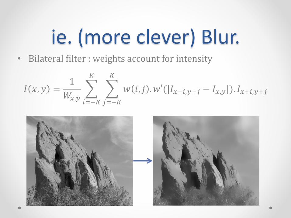
ie. (more clever) Blur.• Bilateral filter : weights account for intensity

𝐼 𝑥, 𝑦 =1

𝑊𝑥,𝑦

𝑖=−𝐾

𝐾

𝑗=−𝐾

𝐾

𝑤 𝑖, 𝑗 . 𝑤′(|𝐼𝑥+𝑖,𝑦+𝑗 − 𝐼𝑥,𝑦|). 𝐼𝑥+𝑖,𝑦+𝑗

Bonus:Motion MagnificationFollowing slides from “Phase-Based Video Motion Processing”,

[Wadhwa et al. 2013]

Goal• Magnify motion:

(That’s using a previous approach)

• For illustration, let’s look at a 1D image profile

Fourier Decomposition

FFT

Space (x)

Inte

nsi

ty

𝐴1 ×

Space (x)

Inte

nsi

ty

+⋯+𝐴2 ×

Inte

nsi

ty

Space (x)

𝑓 𝑥

𝜔=−∞

∞

𝐴𝜔𝑒𝑖𝜔𝑥

FFT

Amplitude of Basis Function

𝐴1 × +𝐴2 × +⋯

𝑆𝜔

Amplitude (𝑆1) Amplitude (𝑆2)

Space (x) Space (x)

Inte

nsi

ty

Inte

nsi

ty

Inte

nsi

ty

Space (x)

FFT

𝑓 𝑥

𝜔=−∞

∞


FFT

• Phase controls location of sinusoid

𝑓 𝑥𝑓 𝑥 − 𝛿

Fourier Shift Theorem

𝐴1 × +𝐴2 × +⋯

𝜔=−∞

∞


FFT

𝑒−𝑖𝜔𝛿

Phase (𝑒−𝑖𝛿) Phase(𝑒−𝑖2𝛿)

Space (x) Space (x)

Inte

nsi

ty

Inte

nsi

ty

Phase Shift ↔ Translation

Inte

nsi

ty

Space (x)

FFT

Local Motions• Fourier shift theorem only lets us

handle global motion

• But, videos have many local motions

• Need a localized Fourier Series for local motion

Mast

Hook

Building

Complex Steerable Pyramid [Simoncelli et al. 1992]

Filter Bank

Orientation 2

Real Imag

Scal

e 1

Orientation 1

Scal

e 2

Orientation 1

Orientation 2Fr

equ

ency

(𝜔𝑦)

Frequency (𝜔𝑥)

Idealized Transfer Functions

Scale

Orientation

FFT

Complex Steerable Pyramid Basis Functions

×

Window

Inte

nsi

ty

Space (x)

Complex Sinusoid (Global)

Inte

nsi

tySpace (x)

Space (x)

Inte

nsi

ty

Single Sub-Band (Scale)• In single scale, image is coefficients times translated copies of

basis functions

𝐴1 × +𝐴2 × +⋯

Single Sub-band of Image Profile

=

Local Amplitude• Local amplitude controls strength of basis function

𝐴1 ×

+𝐴2 × +⋯


=

Local Amplitude

Local Phase• Local phase controls location of sinusoid under window, approximates local

translation

+𝐴2 × +⋯


=

Local Phase

Local Phase Shift ↔ Local Translation

Local Motions

𝐴1 ×

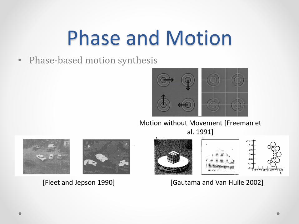
• Phase-based motion synthesis

• Phase-based optical flow

Phase and Motion

[Fleet and Jepson 1990] [Gautama and Van Hulle 2002]

Motion without Movement [Freeman et al. 1991]

Time (t)

Phase over Time

Rad

ian

s

Time (t)

Time (t)

Rad

ian

s

Phase over Time

…

WaveletsInput

Space(x)

Inte

nsi

tyIn

ten

sity

Space(x)

a

Inte

nsi

ty

Space(x)

Phase over Time

Time (t)

Phase over TimeInput Motion-magnified

Space(x)

Rad

ian

s

Time (t)

Time (t)

Rad

ian

s

Space(x)

Inte

nsi

ty

Inte

nsi

ty

…Space(x)

Inte

nsi

tyIn

ten

sity

Space(x)

Wavelets

2D Complex Steerable Pyramid

Filter Bank

Orientation 2

Real Imag

Scal

e 1

Orientation 1

Scal

e 2

Orientation 1

Orientation 2Fr

equ

ency

(𝜔𝑦)

Frequency (𝜔𝑥)

Idealized Transfer Functions

Scale

Orientation

FFT

HipassResidual

LopassResidual

Complex Steerable Pyramid Decomposition

Amplitude

Sub-bands

Filter Bank

Orientation 2

Real Imag

Scal

e 1

Orientation 1

Scal

e 2

Orientation 1

Orientation 2

Phase

Amplitude Phase

𝐴 𝑒𝑖𝜙×

Phase over TimeAmplitude

Sub-bands

Filter Bank

Orientation 2

Real Imag

Scal

e 1

Orientation 1

Scal

e 2

Orientation 1

Orientation 2

Phase

Ph

ase

Time (s)

Phase over time

Ph

ase

Bandpassed Phase over time

Time (s)

Temporal Filtering

New Phase-Based PipelineAmplitude

Sub-bands

Filter Bank

Complex steerable pyramid[Simoncelli et al. 1992]

BandpassedPhase

Orientation 2

Real Imag

Scal

e 1

Orientation 1

Scal

e 2

Orientation 1

Orientation 2

Phase

Rec

on

stru

ctio

n

𝛼 ⊗

𝛼 ⊗

𝛼 ⊗

𝛼 ⊗

Tem

po

ral F

ilter

ing

Temporal filtering on phases

Linear Pipeline (Wu et al. 2012)

Laplacian pyramid[Burt and Adelson 1983] Temporal filtering on intensities

New Phase-Based PipelineAmplitude

Sub-bands

Filter Bank

Complex steerable pyramid[Simoncelli et al. 1992]

BandpassedPhase

Orientation 2

Real Imag

Scal

e 1

Orientation 1

Scal

e 2

Orientation 1

Orientation 2

Phase

Rec

on

stru

ctio

n

𝛼 ⊗

𝛼 ⊗

𝛼 ⊗

𝛼 ⊗

Tem

po

ral F

ilter

ing

Temporal filtering on phases

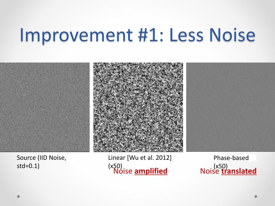
Improvement #1: Less Noise

Noise amplified Noise translated

Source (IID Noise, std=0.1)

Linear [Wu et al. 2012] (x50)

Phase-based (x50)

Improvement #2: More Amplification

Amplification factor Motion in the sequence

Range of linear method:

Range of phase-based method:

4 times theamplification!

Attenuated

• Local phase can move image features, but only within the filter window

Limits of Phase Based Magnification

Amplification factor

See Paper For…• The bound on amplification

• Sub-octave bandwidth pyramid

𝛼𝛿 <𝜆

2

Amplification Initial motion Spatial wavelength

Compact Overcomplete

Comparison with [Wu et al. 2012]

Wu et al. 2012 Phase-Based (this paper)

Vibration due to Camera’s Mirror

Source (300 FPS) Wu et al. 2012 Phase-based (this paper)

Comparison with [Wu et al. 2012] and Video Denoising

Wu et al. with VBM3D

Phase-based (this paper)

Wu et al.

Wu et al. + Liu and Freeman 2010

Talk Overview• Eulerian Video Magnification [Wu et al. SIGGRAPH’12]

o Hao-yu Wu, Michael Rubinstein, Eugene Shih, John Guttag, Frédo Durand, William T. Freeman

• Phase-Based Video Motion Processing [this paper]o Neal Wadhwa, Michael Rubinstein, Frédo Durand, William T. Freeman

• Results, new applications, controlled sequences

Eye Movements

Source (500FPS) Motion magnified x150 (30-50 Hz)

Expressions

Low frequency motions Mid-range frequency motions

Source

Ground Truth Validation

• Induce motion (with hammer)

• Record with accelerometer

AccelerometerHammer Hit

Ground Truth Validation

Qualitative Comparison

Input(motion of 0.1 px)

“Ground truth”(motion of 5 px)

Motion-magnified (x50)

time

space

Motion Attenuation

Source Turbulence Removed

Sequence courtesy Vimeo user Vincent Laforet

Car EngineSource

Car Engine22Hz Magnified

Car EngineSource

Car Engine22Hz Magnified

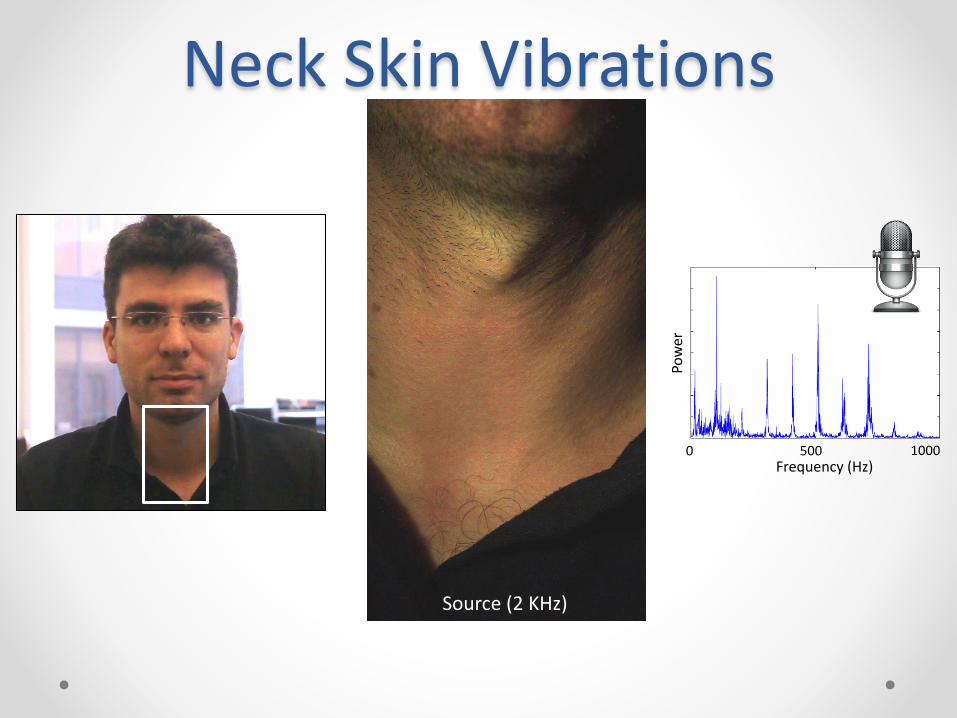
Neck Skin Vibrations

Frequency (Hz)0 500 1000

Pow

er

Source (2 KHz)

Source (2 KHz)

Frequency (Hz)0 500 1000

Pow

er

Source (2 KHz) 100 Hz Amplified x100

Fundamental frequency: ~100Hz

Source (2 KHz) Amplified (x100)

Conclusions• New representation for analyzing and

editing small motions

• Much better than linear EVM [Wu et al. 2012] o Less noiseo More amplification

• Still “Eulerian” (no optical flow), but more explicit representation of motion o New capabilities (e.g. attenuating distracting motions)

LinearSIGGRAPH’12

Phase-basedSIGGRAPH’13

Phase over time

Phase-Based Motion Processing: Code and Web App

• Code available soon: http://people.csail.mit.edu/nwadhwa/phase-video/

http://videoscope.qrclab.com/

http://people.csail.mit.edu/nwadhwa/phase-video/

http://videoscope.qrclab.com/

Overall Conclusion• Many problems involve solving for Poisson equations

o For image editing

o For video processing

o For rendering

o For geometry processing (more with Julie)

• Many solvers existo Iterative solvers (Krylov or not...)

o Direct solvers (Cholesky)

o Fourier, FFT or Green’s function-based

• We have seen other cool image/video applicationso ... though not with Poisson!

Image and video processing - Centre national de la … Bonneel1 James Tompkin2 Kalyan Sunkavalli3...

Documents

Transcript of Image and video processing - Centre national de la … Bonneel1 James Tompkin2 Kalyan Sunkavalli3...