FullText (17)
80
Title On mixed portmanteau statistics for the diagnostic checking of time series models using Gaussian quasi-maximum likelihood approach Advisor(s) Li, G; Li, WK Author(s) Li, Yuan; 李源 Citation Issued Date 2012 URL http://hdl.handle.net/10722/173876 Rights The author retains all proprietary rights, (such as patent rights) and the right to use in future works.
description
thesisi
Transcript of FullText (17)

TitleOn mixed portmanteau statistics for the diagnostic checking oftime series models using Gaussian quasi-maximum likelihoodapproach
Advisor(s) Li, G; Li, WK
Author(s) Li, Yuan; 李源
Citation
Issued Date 2012
URL http://hdl.handle.net/10722/173876
Rights The author retains all proprietary rights, (such as patent rights)and the right to use in future works.
Abstract of thesis entitled
ON MIXED PORTMANTEAU STATISTICS
FOR THE DIAGNOSTIC CHECKING OF
NONLINEAR TIME SERIES USING
GAUSSIAN QUASI-MAXIMUM LIKELIHOOD
APPROACH
Submitted by
Yuan LI
for the degree of Master of Philosophy
at The University of Hong Kong
in September 2012
This thesis aims at investigating different forms of residuals from a general
time series model with conditional mean and conditional variance fitted by the
Gaussian quasi-maximum likelihood method. We investigated the limiting dis-
tributions of autocorrelation and partial autocorrelation functions under differ-
ent forms of residuals. Based on them we devised some individual portmanteau
tests and two mixed portmanteau tests. We started by exploring the asymp-
totic normalities of the residual autocorrelation functions, the squared resid-
ual autocorrelation functions and absolute residual autocorrelation functions
from the fitted time series model. This leads to three individual portmanteau

tests. Then we generalized them to their counterparts of partial autocorrela-
tion functions, and this results in another three individual portmanteau tests.
We carried out simulations studies to compare the six individual portmanteau
tests and find that some tests are sensitive to mis-specification in the condi-
tional mean while other tests are effective to detect mis-specification in the
conditional variance. However, for the case that the mis-specifications happen
in both conditional mean and variance, none of these individual portmanteau
tests present remarkable power. Based on this, we continued to investigate the
joint limiting distributions of the residual autocorrelation functions and ab-
solute residual autocorrelation functions of the fitted model since the former
one is powerful to identify mis-specification in the conditional mean and the
latter one works well when the conditional variance is mis-specified. This leads
to two mixed portmanteau tests for diagnostic checking of the fitted model.
Simulation studies are carried out to check the asymptotic theory and to as-
sess the performance of the mixed portmanteau tests. It shows that the mixed
portmanteau tests have the power to detect mis-specification in the conditional
mean and conditional variance respectively while it is feasible to detect both
of them.

ON MIXED PORTMANTEAU STATISTICS
FOR THE DIAGNOSTIC CHECKING OF
TIME SERIES MODELS USING GAUSSIAN
QUASI-MAXIMUM LIKELIHOOD
APPROACH
by
Yuan LI
A thesis submitted in partial fulfillment of the requirements for
the Degree of Master of Philosophy
at The University of Hong Kong.
September 2012

Declaration
I declare that this thesis represents my own work, except where due ac-
knowledgement is made, and that it has not been previously included in a
thesis, dissertation or report submitted to this University or to any other in-
stitution for a degree, diploma or other qualifications.
Signed....................................................
Yuan LI
i

Acknowledgements
I am indebted to my supervisor Dr. Guodong Li and Professor Wai Keung
Li for providing a pleasant research environment and constant support during
my study. I benefit tremendously from their valuable advices and inspiring
discussions. As my main supervisor, Dr.Guodong Li spent much time in su-
pervising me and has always been so nice and approachable whenever I need
help.
I am very grateful to staff and fellow research postgraduates at the De-
partment of Statistics and Actuarial Sciences, the University of Hong Kong
for their kindness and support. Thanks also go to my friends, especially those
in Morrison Hall. They enrich my life outside research and help me become a
well-rounded person.
My greatest gratitude must be addressed to my beloved parents for their
unconditional love and support. It has been and will always be the major
impetus for me.
ii

Contents
Declaration i
Acknowledgements i
Contents iii
1 Introduction 1
1.1 Diagnostic checking tools in literature . . . . . . . . . . . . . . . 1
1.2 Organization of this thesis . . . . . . . . . . . . . . . . . . . . . 4
2 Some portmanteau tests for time series models by the Gaus-
sian quasi-maximum likelihood estimation 6
2.1 Introduction . . . . . . . . . . . . . . . . . . . . . . . . . . . . . 6
2.2 Models and Assumptions . . . . . . . . . . . . . . . . . . . . . . 9
2.3 Autocorrelation-based Portmanteau Tests . . . . . . . . . . . . 11
2.4 Partial autocorrelation-based Portmanteau Tests . . . . . . . . . 28
2.5 Simulation study of Q1(M) ∼ Q6(M) . . . . . . . . . . . . . . . 34
3 Two Mixed Portmanteau Tests for Time Series using Gaussian
iii
Quasi Maximum Likelihood Estimation 40
3.1 Introduction . . . . . . . . . . . . . . . . . . . . . . . . . . . . . 40
3.2 The mixed portmanteau test Q∗1(2M) based on residual and
absolute residual autocorrelations . . . . . . . . . . . . . . . . . 42
3.3 The mixed portmanteau test Q∗2(2M) based on residual and
squared residual autocorrelations . . . . . . . . . . . . . . . . . 48
3.4 Simulation Study of Q∗1(2M) and Q∗2(2M) . . . . . . . . . . . . 52
4 An Illustrative Example 57
5 Conclusion 65
iv

List of Tables
2.1 Empirical sizes and powers of Q1(M) ∼ Q6(M). . . . . . . . . . 37
3.1 Empirical size and power of Q1(M) ∼ Q6(M), Q∗1(2M) and
Q∗1(2M). . . . . . . . . . . . . . . . . . . . . . . . . . . . . . . . 56
vi

Chapter 1
Introduction
1.1 Diagnostic checking tools in literature
One of the statistician’s main tasks is to come up with a mathematical model
from the statistical perspective that can describe the real data adequately.
Based on the same dataset, statisticians can have different models to describe
it. Therefore, the key question is to choose the model that fits the data well.
The same can be said about time series analysis. In order to do that, some
statistical tests should be designed as the diagnostic tool to check whether
the proposed model is powerful enough for describing the data. Since Karl
Pearson came up with the first diagnostic tools, a chi-squared goodness-of-fit
test, many tests have been suggested.
1
Box and Pierce (1970)’s seminal work has been the foundation of many
diagnostic tools after it. They introduced a portmanteau test, which is the
sum of squares of residual autocorrelations, follows a chi-squared distribution
asymptotically. Since it is an asymptotic result, some modifications can be
implemented to improve the portmanteau test. One of the widely recognized
efforts is done by Ljung and Box (1978). They improved the approximation
by using the standardized autocorrelations to substitute the initial ones in
Box and Pierce’s test statistic. They showed that the new statistic is still
asymptotically chi-squared distributed but the approximation is closer to the
theoretical chi-squared distribution. For linear time series models, Ljung and
Box test is still frequently used today.
However, that is not the end of the story of diagnostic checking for time
series models. Monti (1994) proposed a portmanteau test based on residual
partial autocorrelations, which offered a new perspective since the diagnos-
tic tools before him had all been focused on autocorrelations. Monti’s test
statistic maintained the structure of Ljung-Box’s, replacing residual autocor-
relations with partial autocorrelations. He showed by simulation experiments
that the new portmanteau test was more powerful when the fitted model un-
derestimated the order of the moving average part in the ARMA model.
The dominant status of linear time series models has been shaken by non-
linear time series models during last thirty years. As a result, almost all the
new diagnostic tools have been suggested for nonlinear time series models. Li
2

and Mak (1994) first proposed a portmanteau test for the diagnostic checking
of the fitted ARCH/GARCH type models. However, for nonlinear time series
models other than ARCH/GARCH, new portmanteau tests are still needed.
Based on the fact that Ljung-Box statistic and Li-Mak statistic are sensitive
to lack of fit in the first and second moments of the data structure respectively,
Wong and Ling (2005) proposed a mixed portmanteau statistic by combining
these two statistics. This test statistic can apply to a very general type of
nonlinear time series model.
In addition, the autocorrelations of absolute values of returns for some asset
prices have been discussed in finance literature. That offers us a natural idea to
consider its somewhat counterpart in statistics, absolute residual autocorrela-
tions. In fact, Li and Li (2005) has made their attempt in devising a portman-
teau statistic based on absolute residual autocorrelation in the background of
least absolute deviation estimation for GARCH models. Furthermore, Li and
Li (2008) generalized their results to the ARFRIMA-GARCH model based on
absolute residual autocorrelations using the least absolute deviation methods.
Therefore, while the development in the field of diagnostic checking is going
on stably, there are still some gaps that need to be filled. First, although the
least absolute deviation method obtained some popularity these years, the
mainstream estimation method used in the field of time series is still quasi-
maximum likelihood estimation method, supported by the fact that almost
all the popular statistical software choose Gaussian quasi-maximum likelihood
3

method as default. This drives us to consider the results proposed under the
least absolute deviation method and to derive similar ones under Gaussian
quasi-maximum likelihood method. Second, partial autocorrelation functions
offer us an alternative way to investigate the residuals of the fitted time series
models but so far it is only investigated for the ARMA model. Scare papers
on partial autocorrelation functions have appeared so far. As a result, we are
motivated to consider this tool in nonlinear time series models. Third, in such
a complex world as the one we have, an individual diagnostic test may not
be able to satisfy our need in practice. Each of them shows some advantages
within comparatively narrow conditions. Considering the mixed form of them
may be the possible way to loosen the conditions for the time series models
and the computational power we have today can totally eliminate our worries
about the computation complexity of the mixed tests.
1.2 Organization of this thesis
In this chapter, we have reviewed the development of diagnostic checking tools
in the literature. In Chapter 2, we will first devise three portmanteau tests
based on autocorrelation functions of the residuals, squared residuals and ab-
solute residuals by the Gaussian quasi-maximum likelihood method. Then
we will generalize them by considering the partial autocorrelation functions
4

and further devise another three portmanteau tests. We will compare these
portmanteau tests through simulation experiments and focus on their perfor-
mances in three cases: the conditional mean is mis-specified; the conditional
heteroscedacity is mis-specified; both the conditional mean and conditional
heteroscedacity are mis-specified. In Chapter 3, we will devise two mixed
portmanteau test based on our simulation results in Chapter 2. Again we use
simulation experiments to compare the two mixed portmanteau test together
with the six individual portmanteau tests devised in Chapter 2. Chapter 4 is
an illustrative example to show the usefulness of the mixed portmanteau test
in application. The data we use is the monthly log return of IBM stock based
on the closing price from January 1926 to December 2008. In the end, we
make our final conclusions in Chapter 5.
5

Chapter 2
Some portmanteau tests for time
series models by the Gaussian
quasi-maximum likelihood
estimation
2.1 Introduction
So far, we have found in the literature many portmanteau tests based on
autocorrelations and partial autocorrelations of some forms of residuals from
the fitted ARMA and GARCH models.
Box and Pierce (1970) first devise a portmanteau test for ARMA models
based on residual autocorrelation functions. Ljung and Box (1978) improved
6

the portmanteau test by adjusting the weight on residual autocorrelations at
different lags and their portmanteau test has become the most frequently used
diagnostic checking tool for linear time series models.
The motivation of defining squared residual autocorrelation for diagnostic
checking can date back to Miller (1979). Miller found that the residuals of
a fitted ARMA model did not appear to be autocorrelated but the squared
residual was significantly autocorrelated when modelling a mean series of daily
riverflow. From then on, researchers have found significantly autocorrelation
in squared residuals from numerous hydrological and economic time series fit-
ted by ARMA models, while the traditional residual autocorrelations did not
indicate any model inadequacy.
McLeod and Li (1983) first proposed a portmanteau statistic for the di-
agnostic checking of general ARMA(p, q) models using squared residual au-
tocorrelations. They also found that this diagnostic tool was not sensitive to
the estimation methods used, even though one of the estimation methods they
considered was least square method, which was not robust to outliers.
Li and Mak (1994) extended the portmanteau statistic using squared resid-
ual autocorrelations to the diagnostic checking of non-linear time series with
conditional mean and heteroscedasticity. The model they used could include
the popular ARCH and GARCH model. The estimation method they used
was conditional maximum likelihood method.
Following the work of Peng and Yao (2003), Li and Li (2005) defined the
7

absolute residual autocorrelation and used it to devise a portmanteau test
based on absolute residual autocorrelations and using the least absolute devi-
ation method for the pure GARCH model. Their simulation results indicated
the similar effect of autocorrelations of the squared residuals and the port-
manteau test based on absolute residual autocorrelations seemed to be the
superior one. Li and Li (2008) further investigated the diagnostic tool based
on absolute residual autocorrelations for ARFIMA-GARCH models, which was
a special case for the non-linear time series model with conditional mean and
heteroscedasticity stated above.
In another path, Monti (1994) first considered the residual partial autocor-
relation functions to devise portmanteau tests for ARMA models. He showed
that this kind of portmanteau test was better than those using residual auto-
correlation functions when the mean part was underestimated.
In this section, we will consider the general nonlinear time series with condi-
tional variance in Li and Mak (1994), and examine the potential portmanteau
tests based on different forms of residuals (residuals, absolute residuals and
squared residuals) in terms of both autocorrelation and partial autocorrela-
tion functions. The Gaussian quasi-maximum likelihood estimation method is
employed. We summarize the scenarios in the following table.
8
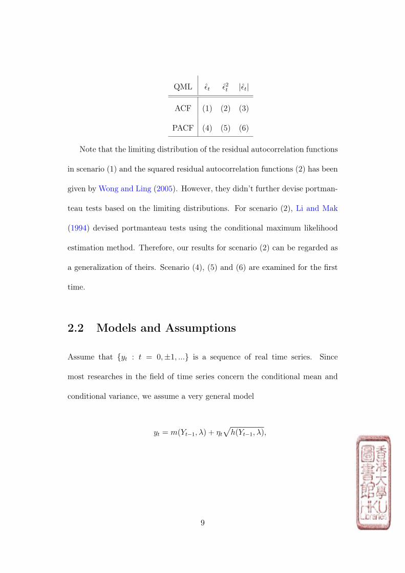
QML εt ε2t |εt|
ACF (1) (2) (3)
PACF (4) (5) (6)
Note that the limiting distribution of the residual autocorrelation functions
in scenario (1) and the squared residual autocorrelation functions (2) has been
given by Wong and Ling (2005). However, they didn’t further devise portman-
teau tests based on the limiting distributions. For scenario (2), Li and Mak
(1994) devised portmanteau tests using the conditional maximum likelihood
estimation method. Therefore, our results for scenario (2) can be regarded as
a generalization of theirs. Scenario (4), (5) and (6) are examined for the first
time.
2.2 Models and Assumptions
Assume that yt : t = 0,±1, ... is a sequence of real time series. Since
most researches in the field of time series concern the conditional mean and
conditional variance, we assume a very general model
yt = m(Yt−1, λ) + ηt√h(Yt−1, λ),
9
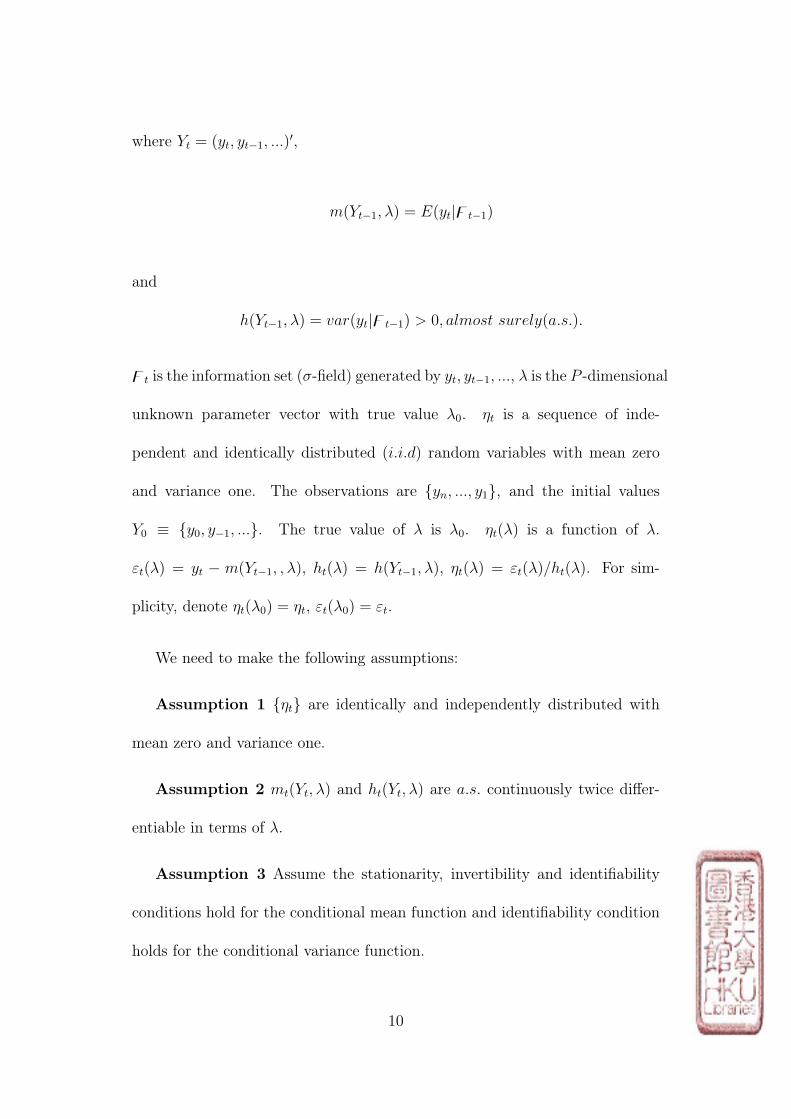
where Yt = (yt, yt−1, ...)′,
m(Yt−1, λ) = E(yt|zt−1)
and
h(Yt−1, λ) = var(yt|zt−1) > 0, almost surely(a.s.).
zt is the information set (σ-field) generated by yt, yt−1, ..., λ is the P -dimensional
unknown parameter vector with true value λ0. ηt is a sequence of inde-
pendent and identically distributed (i.i.d) random variables with mean zero
and variance one. The observations are yn, ..., y1, and the initial values
Y0 ≡ y0, y−1, .... The true value of λ is λ0. ηt(λ) is a function of λ.
εt(λ) = yt − m(Yt−1, , λ), ht(λ) = h(Yt−1, λ), ηt(λ) = εt(λ)/ht(λ). For sim-
plicity, denote ηt(λ0) = ηt, εt(λ0) = εt.
We need to make the following assumptions:
Assumption 1 ηt are identically and independently distributed with
mean zero and variance one.
Assumption 2 mt(Yt, λ) and ht(Yt, λ) are a.s. continuously twice differ-
entiable in terms of λ.
Assumption 3 Assume the stationarity, invertibility and identifiability
conditions hold for the conditional mean function and identifiability condition
holds for the conditional variance function.
10
Assumption 4 εt is strictly stationary and ergodic with finite fourth
order moment, i.e. Eε4t < +∞
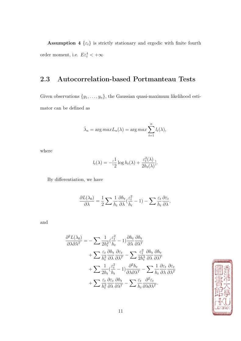
2.3 Autocorrelation-based Portmanteau Tests
Given observations y1, . . . , yn, the Gaussian quasi-maximum likelihood esti-
mator can be defined as
λn = argmaxLn(λ) = argmaxn∑t=1
lt(λ),
where
lt(λ) = −[1
2log ht(λ) +
ε2t (λ)
2ht(λ)].
By differentiation, we have
∂L(λ0)
∂λ=
1
2
∑ 1
ht
∂ht∂λ
(ε2tht− 1)−
∑ εtht
∂εt∂λ
,
and
∂2L(λ0)
∂λ∂λT=−
∑ 1
2h2t(ε2tht− 1)
∂ht∂λ
∂ht∂λT
+∑ εt
h2t
∂ht∂λ
∂εt∂λT
−∑ ε2t
2h3t
∂ht∂λ
∂ht∂λT
+∑ 1
2ht(ε2tht− 1)
∂2ht∂λ∂λT
−∑ 1
ht
∂εt∂λ
∂εt∂λT
+∑ εt
h2t
∂εt∂λ
∂ht∂λT
−∑ εt
ht
∂2εt∂λ∂λT
.
11

By the ergodic theorem, the first, second, fourth, sixth and seventh items
on the right hand side are zero. Therefore, we have
∂2L(λ0)
∂λ∂λT≈ −
∑ ε2tht
1
2h2t
∂ht∂λ
∂ht∂λT
−∑ 1
ht
∂εt∂λ
∂εt∂λT
.
A Taylor expansion of ∂L∂λ
around λ0 estimated at λn yields
0 =∂L(λn)
∂λ≈∂L(λ0)
∂λ+∂2L(λ0)
∂λ∂λT(λn − λ0).
Therefore,
√n(λn − λ0) = −[
1
n
∂2L(λ0)
∂λ∂λT]−1
1√n
∂L(λ0)
∂λ+ op(1).
Denote
Dt =∂lt(λ0)
∂λ=
1
2ht
∂ht∂λ
(ε2tht− 1)− εt
ht
∂εt∂λ
,
and
Σ = − 1
n
∂2L(λ0)
∂λ∂λT=
1
n
∑ 1
2h2t
∂ht∂λ
∂ht∂λT
+1
n
∑ 1
ht
∂εt∂λ
∂εt∂λT
.
Therefore, we can write the estimator λn in the following expansion:
√n(λn − λ0) =
Σ−1√n
n∑t=1
Dt + op(1).
Note thatDt is a martingale difference with respect tozt with E(Dt|zt−1) =
12

0 and E(DtD′t) ≡ Ω. By the Martingale Central Limit Theorem in Billingsley
(1961), it can be shown that
1√n
n∑t=1
Dt → N(0,Ω)
in distribution. Therefore, we directly have
√n(λn − λ0)→ N(0,Σ−1ΩΣ−1)
in distribution.
By a direct calculation, we have
Ω =E[DtD′t]
=κ1E[1
4h2t
∂ht∂λ
∂ht∂λT
] + E[1
ht
∂εt∂λ
∂εt∂λT
]
− κ2E[1
2h3/2t
(∂ht∂λ
∂εt∂λT
+∂εt∂λ
∂ht∂λT
)],
where κ1 = E[(η2t − 1)2] and κ2 = E[(η2t − 1)ηt].
Next, we will investigate the six scenarios one by one in order to devise
a portmanteau test under each scenario. Since there will be many notations
and definition, we will identify similar notations with the same letter with the
number in the upper right to indicate the scenario it belongs to.
13

In scenario (1), residuals are defined as
ηt =εt√ht,
where ηt is short for ηt(λn). εt and ht are similarly defined. Further, the lag-k
standardized residual autocorrelation can be defined in the traditional way as
ρk(1) =
∑nt=k+1(ηt − η1)(ηt−k − η1)∑n
t=1(ηt − η1)2,
where η1 = n−1∑n
t=1 ηt.
Note that
η =1
n
n∑t=1
ηt =1
n
n∑t=1
εt(Yt−1, λn)√ht(Yt−1, λn)
=1
n
n∑t=1
εt(Yt−1, λ0)√ht(Yt−1, λ0)
+∂ηt(Yt−1, λ0)
∂λ(λn − λ0)
=1
n
∑ηt +
1
n
∑ ∂ηt(Yt−1, λ0)
∂λ(λn − λ0).
As a result, we have√nη = Op(1) and n(η)2 = Op(1).
Similarly, it is easy to show that
1
n
n∑t=1
η2t =1
n
n∑t=1
η2t + op(1) = 1 + op(1).
14

Therefore, we only need to consider
√nρk
(1) =n−1/2
∑ηtηt−k −
√n(η)2
n−1∑η2t − (η)2
=n−1/2
∑ηtηt−k
n−1∑η2t
+ op(1)
=1√n
∑ηtηt−k + op(1).
Denote C(1) = (C(1)1 , . . . , C
(1)M ) and ∂C(1)
∂λ= (
∂C(1)1
∂λ, . . . ,
∂C(1)M
∂λ)′, where C(1)
k =
n−1∑ηtηt−k and C(1)
k = n−1∑ηtηt−k. By Taylor expansion, we have
C(1) l C(1) +∂C(1)
∂λ(λn − λ0).
It holds that, for k = 1, . . . ,M,
∂C(1)k
∂λ=− 1
n
∑ ∂mt
∂λ
1√ht
εt−k√ht−k
− 1
2n
∑ εt
h3/2t
∂ht∂λ
εt−k√ht−k
− 1
n
∑ ∂mt−k
∂λ
1√ht−k
εt√ht− 1
2n
∑ εt−k
h3/2t−k
∂ht−k∂λ
εt√ht.
By the ergodic theorem, the last three items on the right-hand side converge
to zero in probability. Hence,
∂C(1)k
∂λ≈ − 1
n
∑ ∂mt
∂λ
ηt−k√ht
≈1
n
∑ ∂εt∂λ
ηt−k√ht.
Denote ρ(1) = (ρ(1)1 , . . . , ρ
(1)M )′ and ρ(1) = (ρ
(1)1 , . . . , ρ
(1)M )′. Therefore, for any
15

given integer M,
√nρ(1) =
√nρ(1) +X(1)
ρ
√n(λn − λ0) + op(1),
where
X(1)ρ = (X
(1)ρ1 , X
(1)ρ2 , . . . , X
(1)ρM)′,
X(1)ρk = E[
∂εt∂λ
ηt−k√ht
], k = 1, 2, . . . ,M.
Based on this result, we have the following theorem under scenario (1).
Theorem 2.1. Under Assumptions 1-4, then
√nρ(1) =
√n(ρ
(1)1 , . . . , ρ
(1)M )′ → N(0, V1),
where
V1 = IM+X(1)ρ Σ−1ΩΣ−1X(1)T
ρ +(κ22X(1)∗ρ −X(1)
ρ )Σ−1X(1)Tρ +X(1)
ρ Σ−1(κ22X(1)∗ρ −X(1)
ρ )T .
Proof of Theorem 1. From above mentioned properties of the Gaussian quasi-
maximum likelihood estimator, we have the following results:
∂L(λ0)
∂λ=
1
2
∑ 1
ht
∂ht∂λ
(ε2tht− 1) +
∑ εtht
∂mt
∂λ,
16

and
√n(λn − λ0)→ N(0,Σ−1ΩΣ−1).
From Theorem 2.8.1 in Lehmann (1998), we can obtain that
√nC(1) → N(0, IM)
in distribution, where IM is the M ×M identity matrix.
Therefore, by Mann-Wald device and Martingale Central Limit Theorem
in Billingsley (1961), C(1) therefore ρ(1) is asymptotically normally distributed.
We need to calculate its covariance matrix,
cov√n(λn − λ0),
√nC(1) = E(Σ−1
∂L
∂λC(1)T ) = Σ−1E(
∂L
∂λC(1)T ).
The expectation of ∂L∂λ
and C(1)k is equal to
n−1E[1
2
∑ 1
ht
∂ht∂λ
(ε2tht− 1) +
∑ εtht
∂mt
∂λ∑ εs√
hs
εs−k√hs−k
].
By taking iterative expectation with respect to zt−1, we find
E[1
2ht
∂ht∂λ
(ε2tht− 1)ηtηt−k] =
κ22X
(1)∗ρk ,
where
X(1)∗ρk = E[
∂ht∂λ
ηt−kht
], k = 1, 2, . . . ,M.
17

Therefore,
E(∂L
∂λC
(1)k ) =
κ22X
(1)∗ρk + n−1E[
∑ εtht
∂mt
∂λ
∑ εs√hs
εs−k√hs−k
]
=κ22X
(1)∗ρk − n
−1∑∑
E[εtht
∂εt∂λ
εs√hs
εs−k√hs−k
]
=κ22X
(1)∗ρk − n
−1∑
E[εtht
∂εt∂λ
εt√ht
εt−k√ht−k
]
=κ22X
(1)∗ρk − E(
ε2tht
)E[∂εt∂(λ)
ηt−k√ht
]
=κ22X
(1)∗ρk −X
(1)ρk .
Denote X(1)∗ρ = (X
(1)∗ρ1 , X
(1)∗ρ2 , . . . , X
(1)∗ρM )′. Then
cov√n(λn − λ0),
√nC(1) = Σ−1E(
∂L
∂λC(1)T ) = Σ−1(
κ22X(1)∗ρ −X(1)
ρ )T .
Therefore, the covariance matrix of√nρ(1) is
var(√nρ(1)) = var(
√nC(1))
=var(√nC(1)) + var(X(1)
ρ
√n(λn − λ0))
+ cov(√nC(1), X(1)
ρ
√n(λn − λ0)) + cov(X(1)
ρ
√n(λn − λ0),
√nC(1))
=IM +X(1)ρ Σ−1ΩΣ−1X(1)T
ρ
+ (κ22X(1)∗ρ −X(1)
ρ )Σ−1X(1)Tρ +X(1)
ρ Σ−1(κ22X(1)∗ρ −X(1)
ρ )T .
This completes the proof.
From the above theorem, we can directly devise the following portmanteau
18

test:
Q1(M) = nρ(1)T V1−1ρ(1) ∼ χ2(M),
where V1 is the estimated value when X(1)ρ , X(1)∗
ρ , Σ and Ω are estimated by
the respective sample averaging.
For scenario (2), similar to Li and Mak (1994), we can prove the following
theorem. Note that their result is based on conditional maximum likelihood
estimation, unlike the quasi-maximum likelihood estimation we employ. See
also Wong and Ling (2005).
In scenario (2), the squared residuals are defined as
η2t =ε2t
ht.
Further, the lag-k standardized squared residual autocorrelation can be defined
in the way in Li and Mat (1994) as
ρk(2) =
∑nt=k+1(η
2t − η2)(η2t−k − η2)∑nt=1(η
2t − η2)2
,
where η2 = n−1∑n
t=1 η2t .
Similar to the argument in scenario (1), if this model is correct, we have
η2 = µ2 + op(1) = 1 + op(1),1
n
n∑t=1
(η2t − η2)2 = σ22 + op(1),
where µ2 = Eη2t , and σ22 = var(η2t ).
19

Therefore, we only need to consider
ρk(2) =
1
nσ22
n∑t=k+1
(η2t − 1)(η2t−k − 1).
Denote C(2) = (C(2)1 , . . . , C
(2)M ) and ∂C(2)
∂λ= (
∂C(2)1
∂λ, . . . ,
∂C(2)M
∂λ)′, where C(2)
k =
n−1∑
(η2t−1)(η2t−k−1) and Ck = n−1∑
(η2t−1)(η2t−k−1). By Taylor expansion,
we have
C(2) ≈ C(2) +∂C(2)
∂λ(λn − λ0).
It holds that, for k = 1, . . . ,M,,
∂Ck∂λ
= − 1
n
∑ η2tht
∂ht∂λ
(ε2t−kht−k
− 1).
Denote ρ(2) = (ρ(2)1 , . . . , ρ
(2)M )′ and ρ(2) = (ρ
(2)1 , . . . , ρ
(2)M )′. Therefore, for any
given integer M,
√nρ(2) =
√nρ(2) + σ−22 X(2)
ρ
√n(λn − λ0) + op(1),
where
X(2)ρ = (X
(2)ρ1 , X
(2)ρ2 , . . . , X
(2)ρM)′,
X(2)ρk = E[
1
ht
∂ht∂λ
(1− η2t−k)], k = 1, 2, . . . ,M.
Based on this result, we have the following theorem under scenario (2).
20
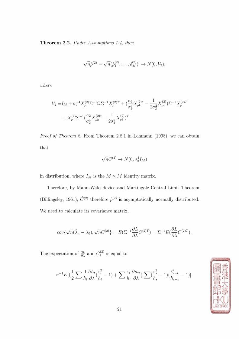
Theorem 2.2. Under Assumptions 1-4, then
√nρ(2) =
√n(ρ
(2)1 , . . . , ρ
(2)M )′ → N(0, V2),
where
V2 =IM + σ−42 X(2)ρ Σ−1ΩΣ−1X(2)T
ρ + (κ2σ42
X(2)∗ρk −
1
2σ22
X(2)ρk )Σ−1X(2)T
ρ
+X(2)ρ Σ−1(
κ2σ42
X(2)∗ρk −
1
2σ22
X(2)ρk )T .
Proof of Theorem 2. From Theorem 2.8.1 in Lehmann (1998), we can obtain
that
√nC(2) → N(0, σ4
2IM)
in distribution, where IM is the M ×M identity matrix.
Therefore, by Mann-Wald device and Martingale Central Limit Theorem
(Billingsley, 1961), C(2) therefore ρ(2) is asymptotically normally distributed.
We need to calculate its covariance matrix,
cov√n(λn − λ0),
√nC(2) = E(Σ−1
∂L
∂λC(2)T ) = Σ−1E(
∂L
∂λC(2)T ).
The expectation of ∂L∂λ
and C(2)k is equal to
n−1E[1
2
∑ 1
ht
∂ht∂λ
(ε2tht− 1) +
∑ εtht
∂mt
∂λ∑
(ε2shs− 1)(
ε2s−khs−k
− 1)].
21

By taking iterative expectation with respect to zt−1, we have
E[εtht
∂mt
∂λ(η2t − 1)(η2t−k − 1)] = κ2X
(2)∗ρk ,
where
X(2)∗ρk = E[
1√ht
∂εt∂λ
(1− η2t−k)], k = 1, 2, . . . ,M.
Also,
n−1E[∑ 1
2ht
∂ht∂λ
(ε2tht− 1)
∑(ε2shs− 1)(
ε2s−khs−k
− 1)]
=n−1∑∑
E[1
2ht
∂ht∂λ
(ε2tht− 1)(
ε2shs− 1)(
ε2s−khs−k
− 1)]
=n−1∑
E[1
2ht
∂ht∂λ
(ε2tht− 1)(
ε2tht− 1)(
ε2t−kht−k
− 1)]
=E[σ22
2ht
∂ht∂λ
(η2t−k − 1)]
=− σ22
2X
(2)ρk .
Therefore,
E[∂L
∂λC
(2)k ] = −σ
22
2X
(2)ρk + κ2X
(2)∗ρk .
Denote X(2)∗ρ = (X
(2)∗ρ1 , X
(2)∗ρ2 , . . . , X
(2)∗ρM )′. Then
cov√n(λn − λ0),
√nC(2) = Σ−1(κ2X
(2)∗ρ − σ2
2
2X(2)ρ )T .
22

Therefore, the covariance matrix of√nρ(2) is
var(√nρ(2)) = σ−42 var(
√nC(2))
=σ−42 [var(√nC(2)) + var(X(2)
ρ
√n(λn − λ0))
+ cov(√nC(2), X(2)
ρ
√n(λn − λ0)) + cov(X(2)
ρ
√n(λn − λ0),
√nC(2))]
=IM + σ−42 X(2)ρ Σ−1ΩΣ−1X(2)T
ρ
+ (κ2σ42
X(2)∗ρk −
1
2σ22
X(2)ρk )Σ−1X(2)T
ρ +X(2)ρ Σ−1(
κ2σ42
X(2)∗ρk −
1
2σ22
X(2)ρk )T .
This completes the proof.
From the above theorem, we can directly devise the following portmanteau
test:
Q2(M) = nρ(2)T V2−1ρ(2) ∼ χ2(M),
where V2 is the estimated value when X(2)ρ , X(2)∗
ρ , Σ and Ω are estimated by
the respective sample averaging.
In scenario (3), the absolute standardized residual is defined as
|ηt| =|εt|√ht.
As usual, |ηt| is short for |ηt(λn)|, where λn is the Gaussian quasi-maximum
likelihood estimator. The lag-k absolute standardized residual autocorrelation
23

can be defined as in Li and Li (2005)
ρk =
∑nt=k+1(|ηt| − η3)(|ηt−k| − η3)∑n
t=1(|ηt| − η3)2,
where η3 = n−1∑n
t=1 |ηt|. If this model is correct, we have
η3 = µ3 + op(1),1
n
n∑t=1
(|ηt| − η3)2 = σ23 + op(1),
where µ3 = E|ηt|, and σ23 = var(|ηt|). Therefore, we only need to consider
ρk(3) =
1
nσ23
n∑t=k+1
(|ηt| − µ3)(|ηt−k| − µ3).
Denote C(3) = (C(3)1 , . . . , C
(3)M ), where
C(3)k =
1
n
n∑t=k+1
(| εt√ht| − µ3)(|
εt−k√ht−k| − µ3).
C(3)k is defined similarly when λ is taken as the Gaussian quasi-maximum like-
lihood estimator λn.
However, when the conditional mean function m(Yt−1, λ) is nonzero, for
the lag-k sample standardized absolute residual autocorrelation function, the
vector C is a function of λn and this function may not be smooth. Therefore
the classic Taylor expansion cannot be used here. We consider a similar form
as Taylor’s expansion of Ck around λ0 estimated at λn.
Denote ρ(3) = (ρ(3)1 , . . . , ρ
(3)M )′ and ρ(3) = (ρ
(3)1 , . . . , ρ
(3)M )′. Following the
24

result of Li and Li (2008), we have:
√nρ(3) =
√nρ(3) − σ−23 X(3)
ρ
√n(λn − λ0) + op(1),
where
X(3)ρ = (X
(3)ρ1 , X
(3)ρ2 , . . . , X
(3)ρM)′,
and
X(3)ρk = E[
1
2ht
∂ht∂λ
(|ηt−k| − µ3)], k = 1, 2, . . . ,M.
Then we can construct its asymptotic distribution.
Theorem 2.3. Under Assumptions 1-4, then
√nρ(3) =
√n(ρ
(3)1 , . . . , ρ
(3)M )′ → N(0, V3),
where
V3 =IM + σ−43 [X(3)ρ Σ−1ΩΣ−1X(3)T
ρ
− (κ3X(3)ρ − 2κ4X
(3)∗ρ )Σ−1X(3)T
ρ −X(3)ρ Σ−1(κ3X
(3)ρ − 2κ4X
(3)∗ρ )T ].
Proof of Theorem 3. From Theorem 2.8.1 in Lehmann (1998), we can obtain
that
√nC → N(0, σ4
3IM)
in distribution, where IM is the M ×M identity matrix.
25
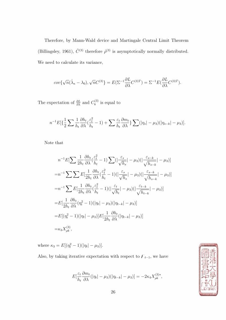
Therefore, by Mann-Wald device and Martingale Central Limit Theorem
(Billingsley, 1961), C(3) therefore ρ(3) is asymptotically normally distributed.
We need to calculate its variance,
cov√n(λn − λ0),
√nC(3) = E(Σ−1
∂L
∂λC(3)T ) = Σ−1E(
∂L
∂λC(3)T ).
The expectation of ∂L∂λ
and C(3)k is equal to
n−1E[1
2
∑ 1
ht
∂ht∂λ
(ε2tht− 1) +
∑ εtht
∂mt
∂λ∑
(|ηs| − µ3)(|ηs−k| − µ3)].
Note that
n−1E[∑ 1
2ht
∂ht∂λ
(ε2tht− 1)
∑(| εs√
hs| − µ3)(|
εs−k√hs−k| − µ3)]
=n−1∑∑
E[1
2ht
∂ht∂λ
(ε2tht− 1)(| εs√
hs| − µ3)(|
εs−k√hs−k| − µ3)]
=n−1∑
E[1
2ht
∂ht∂λ
(ε2tht− 1)(| εt√
ht| − µ3)(|
εt−k√ht−k| − µ3)]
=E[1
2ht
∂ht∂λ
(η2t − 1)(|ηt| − µ3)(|ηt−k| − µ3)]
=E[(η2t − 1)(|ηt| − µ3)]E[1
2ht
∂ht∂λ
(|ηt−k| − µ3)]
=κ3X(3)ρk ,
where κ3 = E[(η2t − 1)(|ηt| − µ3)].
Also, by taking iterative expectation with respect to zt−1, we have
E[εtht
∂mt
∂λ(|ηt| − µ3)(|ηt−k| − µ3)] = −2κ4X
(3)∗ρk ,
26

where κ4 = E[ηt(|ηt| − µ3)], and
X(3)∗ρk = E[
1
2√ht
∂εt∂λ
(|ηt−k| − µ3)], k = 1, 2, . . . ,M.
Therefore,
E[∂L
∂λC
(3)k ] = κ3X
(3)ρk − 2κ4X
(3)∗ρk .
Denote X(3)∗ρ = (X
(3)∗ρ1 , X
(3)∗ρ2 , . . . , X
(3)∗ρM )′. Then
cov√n(λn − λ0),
√nC = Σ−1(κ3X
(3)ρ − 2κ4X
(3)∗ρ )T .
Therefore, the covariance matrix of√nρ(3) is
var(√nρ(3)) = σ−43 var(
√nC(3))
=σ−43 [var(√nC(3)) + var(X(3)
ρ
√n(λn − λ0))
− cov(√nC(3), X(3)
ρ
√n(λn − λ0))− cov(X(3)
ρ
√n(λn − λ0),
√nC(3))]
=IM + σ−43 [X(3)ρ Σ−1ΩΣ−1X(3)T
ρ
− (κ3X(3)ρ − 2κ4X
(3)∗ρ )Σ−1X(3)T
ρ −X(3)ρ Σ−1(κ3X
(3)ρ − 2κ4X
(3)∗ρ )T ].
This completes the proof.
Then we can devise the portmanteau test under scenario (3)
Q3(M) = nρ(3)T V3−1ρ(3) ∼ χ2(M),
27
where V3 is the estimated value when X(3)ρ , X(3)∗
ρ , Σ and Ω are estimated by
the respective sample averaging.
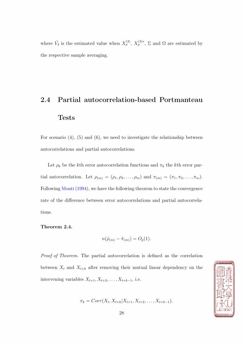
2.4 Partial autocorrelation-based Portmanteau
Tests
For scenario (4), (5) and (6), we need to investigate the relationship between
autocorrelations and partial autocorrelations.
Let ρk be the kth error autocorrelation functions and πk the kth error par-
tial autocorrelation. Let ρ(m) = (ρ1, ρ2, . . . , ρm) and π(m) = (π1, π2, . . . , πm).
Following Monti (1994), we have the following theorem to state the convergence
rate of the difference between error autocorrelations and partial autocorrela-
tions.
Theorem 2.4.
n(ρ(m) − π(m)) = Op(1).
Proof of Theorem. The partial autocorrelation is defined as the correlation
between Xt and Xt+k after removing their mutual linear dependency on the
intervening variables Xt+1, Xt+2, . . . , Xt+k−1, i.e.
πk = Corr(Xt, Xt+k|Xt+1, Xt+2, . . . , Xt+k−1).
28

Without loss of generality, we assume E(Xt) = 0. Let the linear depen-
dency of Xt+k on Xt+1, Xt+2, . . . , Xt+k−1 be defined as the best linear estimate
in the sense of mean square:
Xt+k = α1Xt+k−1 + α2Xt+k−2 + · · ·+ αk−1Xt+1,
where αi (1 ≤ i ≤ k − 1) are obtained by minimizing
E(Xt+k − Xt+k)2 = E(Xt+k − α1Xt+k−1 − α2Xt+k−2 − · · · − αk−1Xt+1)
2.
By differentiation, we have
γi = α1γi−1 + α2γi−2 + · · ·+ αk−1γi−k+1, 1 ≤ i ≤ k − 1,
where γi = cov(Xt, Xt+i).
Hence,
ρi = α1ρi−1 + α2ρi−2 + · · ·+ αk−1ρi−k+1, 1 ≤ i ≤ k − 1.
Similarly,
Xt = β1Xt+1 + β2Xt+2 + · · ·+ βk−1Xt+k−1,
29

where βi (1 ≤ i ≤ k − 1) are obtained by minimizing
E(Xt − Xt)2 = E(Xt − β1Xt+1 − β2Xt+2 − · · · − βk−1Xt+k−1)
2.
Hence,
ρi = β1ρi−1 + β2ρi−2 + · · ·+ βk−1ρi−k+1, 1 ≤ i ≤ k − 1.
Therefore, we have αi = βi (1 ≤ i ≤ k − 1).
Now, we calculate
var(Xt − Xt)
=E[(Xt+k − α1Xt+k−1 − α2Xt+k−2 − · · · − αk−1Xt+1)2]
=E[Xt+k(Xt+k − α1Xt+k−1 − α2Xt+k−2 − · · · − αk−1Xt+1)]
− α1E[Xt+k−1(Xt+k − α1Xt+k−1 − α2Xt+k−2 − · · · − αk−1Xt+1)]
− · · · − αk−1E[Xt+k−1(Xt+1 − α1Xt+k−1 − α2Xt+k−2 − · · · − αk−1Xt+1)]
=E[Xt+k(Xt+k − α1Xt+k−1 − α2Xt+k−2 − · · · − αk−1Xt+1)]
=γ0 − α1γ1 − · · · − αk−1γk−1,
30

and
cov[(Xt − Xt), (Xt+k − Xt+k)]
=E[(Xt − α1Xt+1 − · · · − αk−1Xt+k−1)(Xt+k − α1Xt+ k − 1− · · · − αk−1Xt+1)]
=E[(Xt − α1Xt+1 − α2Xt+2 − · · · − αk−1Xt+k−1)Xt+k]
=γk − α1γk−1 − · · · − αk−1γ1.
Therefore,
πk =cov[(xt − xt), (xt+k − xt+k)]√var(xt − xt)
√var(xt+k − xt+k)
=ρk − α1ρk−1 − · · · − αk−1ρ11− α1ρ1 − · · · − αk−1ρk−1
.
Then,
πk = ψk(ρ(k)) =ρk − ρ
′
(k−1)R−1(k−1)ρ
∗(k−1)
1− ρk − ρ′(k−1)R
−1(k−1)ρ(k−1)
,
whereR(k) = (ρ|i−j|)i,j=1,2,...,k, and ρ∗(k−1) = (ρk, ρk−1, . . . , ρ1)′ . See also Monti(1994).
Now if the error autocorrelations are zero, then
ρk = Op(n− 1
2 ).
Further,
R(k) = Ik +Op(n− 1
2 ).
Therefore, we have
π(m) = ρ(m) +Op(n− 1
2 ),
31
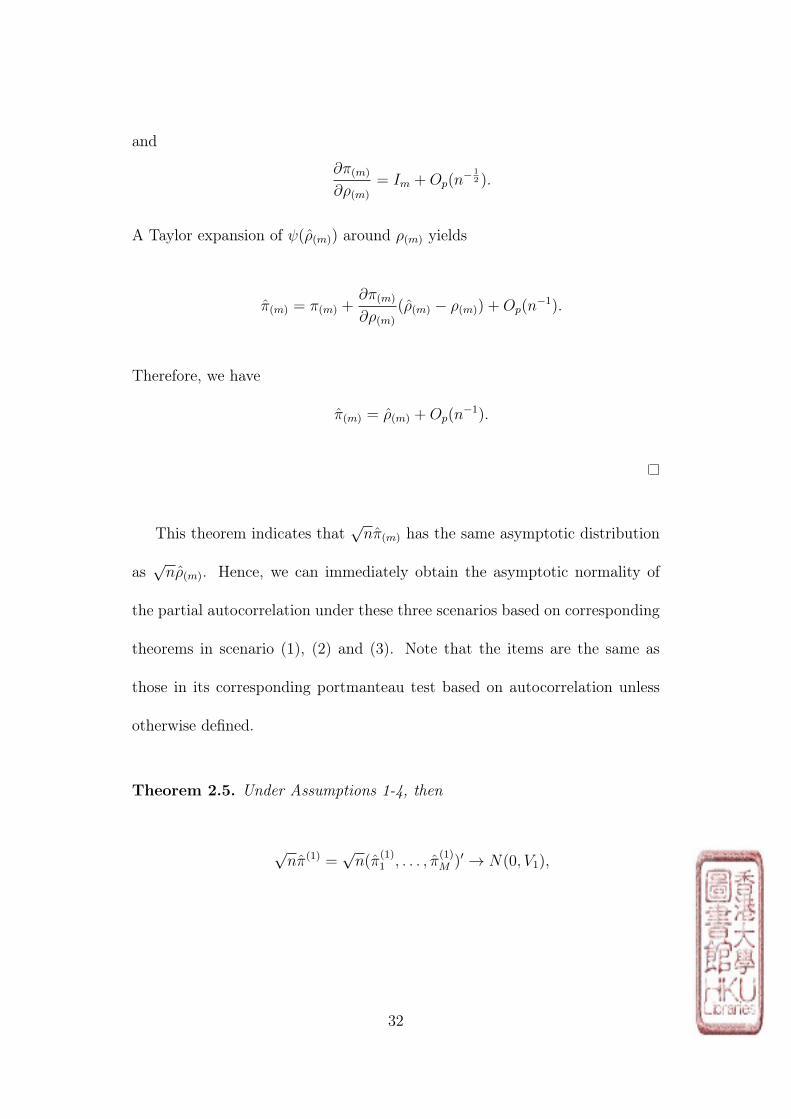
and
∂π(m)
∂ρ(m)
= Im +Op(n− 1
2 ).
A Taylor expansion of ψ(ρ(m)) around ρ(m) yields
π(m) = π(m) +∂π(m)
∂ρ(m)
(ρ(m) − ρ(m)) +Op(n−1).
Therefore, we have
π(m) = ρ(m) +Op(n−1).
This theorem indicates that√nπ(m) has the same asymptotic distribution
as√nρ(m). Hence, we can immediately obtain the asymptotic normality of
the partial autocorrelation under these three scenarios based on corresponding
theorems in scenario (1), (2) and (3). Note that the items are the same as
those in its corresponding portmanteau test based on autocorrelation unless
otherwise defined.
Theorem 2.5. Under Assumptions 1-4, then
√nπ(1) =
√n(π
(1)1 , . . . , π
(1)M )′ → N(0, V1),
32

where
V1 = IM+X(1)ρ Σ−1ΩΣ−1X(1)T
ρ +(κ22X(1)∗ρ −X(1)
ρ )Σ−1X(1)Tρ +X(1)
ρ Σ−1(κ22X(1)∗ρ −X(1)
ρ )T .
Theorem 2.6. Under Assumptions 1-4, then
√nπ(2) =
√n(π
(2)1 , . . . , π
(2)M )′ → N(0, V2),
where
V2 =IM + σ−42 X(2)ρ Σ−1ΩΣ−1X(2)T
ρ + (κ2σ42
X(2)∗ρk −
1
2σ22
X(2)ρk )Σ−1X(2)T
ρ
+X(2)ρ Σ−1(
κ2σ42
X(2)∗ρk −
1
2σ22
X(2)ρk )T .
Theorem 2.7. Under Assumptions 1-4, then
√nπ(3) =
√n(π
(3)1 , . . . , π
(3)M )′ → N(0, V3),
where
V3 =IM + σ−43 [X(3)ρ Σ−1ΩΣ−1X(3)T
ρ
− (κ3X(3)ρ − 2κ4X
(3)∗ρ )Σ−1X(3)T
ρ −X(3)ρ Σ−1(κ3X
(3)ρ − 2κ4X
(3)∗ρ )T ].
Therefore, we can devise another three portmanteau tests based on partial
33
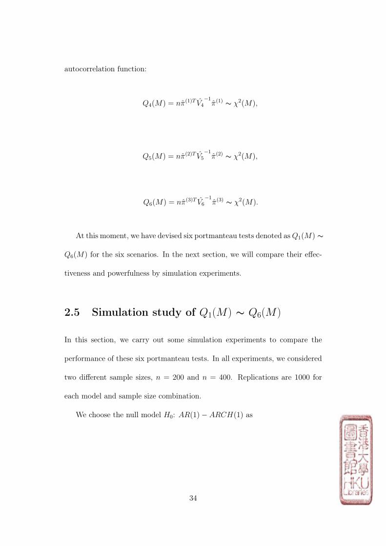
autocorrelation function:
Q4(M) = nπ(1)T V4−1π(1) ∼ χ2(M),
Q5(M) = nπ(2)T V5−1π(2) ∼ χ2(M),
Q6(M) = nπ(3)T V6−1π(3) ∼ χ2(M).
At this moment, we have devised six portmanteau tests denoted asQ1(M) ∼
Q6(M) for the six scenarios. In the next section, we will compare their effec-
tiveness and powerfulness by simulation experiments.
2.5 Simulation study of Q1(M) ∼ Q6(M)
In this section, we carry out some simulation experiments to compare the
performance of these six portmanteau tests. In all experiments, we considered
two different sample sizes, n = 200 and n = 400. Replications are 1000 for
each model and sample size combination.
We choose the null model H0: AR(1)− ARCH(1) as
34

yt = 0.5yt−1 + εt,
εt = ηt√ht,
ht = 0.01 + 0.4ε2t−1.
(2.5.1)
The following three alternative models are considered to investigate the
powers of each portmanteau test. H1(1):AR(2)− ARCH(1):
yt = 0.5yt−1 + 0.2yt−2 + εt,
εt = ηt√ht,
ht = 0.01 + 0.4ε2t−1.
(2.5.2)
H1(2):AR(1)− ARCH(2):
yt = 0.5yt−1 + εt,
εt = ηt√ht,
ht = 0.01 + 0.4ε2t−1 + 0.3ε2t−2.
(2.5.3)
H1(3):AR(2)− ARCH(2):
yt = 0.5yt−1 + 0.1yt−2 + εt,
εt = ηt√ht,
ht = 0.01 + 0.4ε2t−1 + 0.2ε2t−2.
(2.5.4)
Note that the three alternative models represent the mean mis-specification,
variance mis-specification, mean and variance mis-specification jointly, respec-
35

tively.
We choose M = 6 as that in Li and Mat (1994). The percentage of re-
jections is based on the upper 5th percentile of the presumed χ2 distributions
with the degrees of freedom 6. The result is summarized in Table 2.1.
36
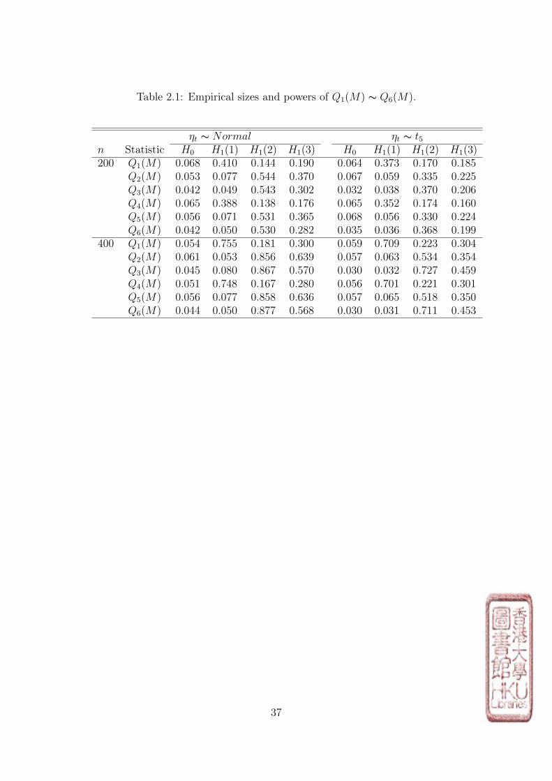
Table 2.1: Empirical sizes and powers of Q1(M) ∼ Q6(M).
ηt ∼ Normal ηt ∼ t5n Statistic H0 H1(1) H1(2) H1(3) H0 H1(1) H1(2) H1(3)200 Q1(M) 0.068 0.410 0.144 0.190 0.064 0.373 0.170 0.185
Q2(M) 0.053 0.077 0.544 0.370 0.067 0.059 0.335 0.225Q3(M) 0.042 0.049 0.543 0.302 0.032 0.038 0.370 0.206Q4(M) 0.065 0.388 0.138 0.176 0.065 0.352 0.174 0.160Q5(M) 0.056 0.071 0.531 0.365 0.068 0.056 0.330 0.224Q6(M) 0.042 0.050 0.530 0.282 0.035 0.036 0.368 0.199
400 Q1(M) 0.054 0.755 0.181 0.300 0.059 0.709 0.223 0.304Q2(M) 0.061 0.053 0.856 0.639 0.057 0.063 0.534 0.354Q3(M) 0.045 0.080 0.867 0.570 0.030 0.032 0.727 0.459Q4(M) 0.051 0.748 0.167 0.280 0.056 0.701 0.221 0.301Q5(M) 0.056 0.077 0.858 0.636 0.057 0.065 0.518 0.350Q6(M) 0.044 0.050 0.877 0.568 0.030 0.031 0.711 0.453
37
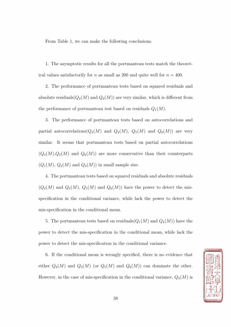
From Table 1, we can make the following conclusions.
1. The asymptotic results for all the portmanteau tests match the theoret-
ical values satisfactorily for n as small as 200 and quite well for n = 400.
2. The performance of portmanteau tests based on squared residuals and
absolute residuals(Q2(M) and Q3(M)) are very similar, which is different from
the performance of portmanteau test based on residuals Q1(M).
3. The performance of portmanteau tests based on autocorrelations and
partial autocorrelations(Q2(M) and Q3(M), Q5(M) and Q6(M)) are very
similar. It seems that portmanteau tests based on partial autocorrelations
(Q4(M),Q5(M) and Q6(M)) are more conservative than their counterparts
(Q1(M), Q2(M) and Q3(M)) in small sample size.
4. The portmanteau tests based on squared residuals and absolute residuals
(Q2(M) and Q3(M), Q5(M) and Q6(M)) have the power to detect the mis-
specification in the conditional variance, while lack the power to detect the
mis-specification in the conditional mean.
5. The portmanteau tests based on residuals(Q1(M) and Q4(M)) have the
power to detect the mis-specification in the conditional mean, while lack the
power to detect the mis-specification in the conditional variance.
6. If the conditional mean is wrongly specified, there is no evidence that
either Q2(M) and Q3(M) (or Q5(M) and Q6(M)) can dominate the other.
However, in the case of mis-specification in the conditional variance, Q3(M) is
38

superior to Q2(M) in terms of power. Similarly, Q6(M) is superior to Q5(M)
in terms of power.
7. When the sample size becomes larger, the powers of all portmanteau
tests increase.
8. The distribution of ηt does not affect all the conclusions above.
Based on the simulation study in this section, a natural idea is to devise a
mixed portmanteau test in order to be effective in the joint mis-specification
in both conditional mean and variance. Although portmanteau tests based on
partial autocorrelation are more robust in smaller sample size, in the following
chapter we will only consider portmanteau tests based on autocorrelation due
to its simple calculations. However, if in practice the sample size is small (less
than 200), we can directly generalize the results in next chapter to the case of
partial autocorrelations.
39

Chapter 3
Two Mixed Portmanteau Tests for
Time Series using Gaussian Quasi
Maximum Likelihood Estimation
3.1 Introduction
For the non-linear time series model with conditional mean and heteroscedas-
ticity, the diagnostic checking for conditional heteroscedasticity is only one
aspect and the diagnostic checking for conditional mean still needs consider-
ation. Fortunately we already have many powerful diagnostic checking tools
for the conditional mean. One natural idea is to view conditional mean and
heteroscedasticity as a package and devise a mixed portmanteau statistics to
test them at the same time. Wong and Ling (2005) first made their attempt
40

and showed that their mixed portmanteau test could be simplified as a direct
summation of Ljung-Box statistic and Li-Mak statistic under some conditions.
In this chapter, we focus on the diagnostic checking for conditional vari-
ance since modeling conditional heteroscedasticity is an important issue for-
ever in economic and financial time series. The autoregressive conditional
heteroscedasticity (ARCH) model proposed by Engle (1982) and the general-
ized autoregressive conditional heteroscedasticity (GARCH) model proposed
by Bollerslev (1986) have achieved great success. From then on, many exten-
sions of GARCH models have appeared in literature. Many of these models
assume the errors are normally distributed so that parameter estimation can
be obtained directly by maximizing the explicit conditional likelihood func-
tion, but it contradicts with the general fact that the distribution of errors is
unknown in real practice. Therefore the Gaussian quasi-maximum likelihood
estimation has been proposed. Weiss (1986) established the asymptotic dis-
tribution of quasi-maximum likelihood estimator for general ARCH(p) model.
For the general GARCH(p, q), Hall and Yao (2003) investigated the asymp-
totic properties of the Gaussian quasi-maximum likelihood estimator.
Based on our simulation experiments in chapter 2, we will construct a mixed
portmanteau test based on residual and absolute residual autocorrelation func-
tions using the Gaussian quasi-maximum likelihood estimation method.
41

3.2 The mixed portmanteau test Q∗1(2M) based
on residual and absolute residual autocorre-
lations
Consider the same model as that in chapter 2.
yt = m(Yt−1, λ) + ηt√h(Yt−1, λ),
where Yt = (yt, yt−1, ...)′,
m(Yt−1, λ) = E(yt|zt−1)
and
h(Yt−1, λ) = var(yt|zt−1) > 0, almost surely(a.s.)
yt : t = 0,±1, ... is a sequence of real time series. zt is the information set
(σ-field) generated by yt, yt−1, .... ηt is a sequence of independent and iden-
tically distributed (i.i.d) random variables with mean zero and variance one.
The observations are yn, ..., y1, and the initial values Y0 ≡ y0, y−1, .... The
parameter λ is (r+s)-dimension with r unknown parameters in the conditional
mean part and s unknown parameters in the conditional variance part. The
true value of λ is λ0. For simplicity, denote ηt(λ0) = ηt, εt(λ0) = εt.
42

Again, we make same assumptions as those in chapter 2.
To maintain consistence with those in chapter 2, we will use the same
notations in this chapter unless pointing out otherwise.
From the results in chapter 2, for the lag-k standardized residual autocor-
relation function, we only need to consider the asymptotic distribution of
√nρ
(1)k =
1√n
∑ηtηt−k + op(1).
Under the Assumptions 1-4,
√nρ(1) =
√nρ(1) +X(1)
ρ
√n(λn − λ0) + op(1)
for any given integer M , where
√nρ
(1)k =
1√n
∑ηtηt−k + op(1),
X(1)ρ = (X
(1)ρ1 , X
(1)ρ2 , . . . , X
(1)ρM)′,
X(1)ρk = E[
∂εt(λ0)
∂(λ)
ηt−k√ht
], k = 1, 2, . . . ,M.
For the lag-k standardized absolute residual autocorrelation, we only need
to consider the asymptotic distribution of
√nρk
(3) =1√nσ2
3
n∑t=k+1
(ηt − µ3)(ηt−k − µ3),
43

where µ3 = E|ηt|, and σ23 = var(|ηt|).
Under Assumptions 1-4,
√nρ(3) =
√nρ(3) − σ−23 X(3)
ρ
√n(λn − λ0) + op(1)
for any given integer M , where
ρ(3)k =
1
nσ23
n∑t=k+1
(| εt√ht| − µ3)(|
εt−k√ht−k| − µ3),
X(3)ρ = (X
(3)ρ1 , X
(3)ρ2 , . . . , X
(3)ρM)′,
X(3)ρk = E[
1
2ht
∂ht∂λ
(|ηt−k| − µ3)], k = 1, 2, . . . ,M.
Also note the following expansion in chapter 2:
√n(λn − λ0) =
Σ−1√n
n∑t=1
Dt + op(1),
where
Dt =∂lt(λ0)
∂λ=
1
2ht
∂ht∂λ
(ε2tht− 1)− εt
ht
∂εt∂λ
and
Σ = − 1
n
∂2L(λ0)
∂λ∂λT=
1
n
∑ 1
2h2t
∂ht∂λ
∂ht∂λT
+1
n
∑ 1
ht
∂εt∂λ
∂εt∂λT
.
44

From all the above results, we have the following theorem about the joint
distribution of ρ(1) and ρ(3):
Theorem 3.1. If all assumptions hold, then,
√n
ρ(1)ρ(3)
→ N(0, P1Ω1PT1 ).
Proof of Theorem. It follows that
√n
ρ(1)ρ(3)
=√nP1
ρ(1)
ρ(3)
1n
∑nt=1Dt
+ op(1),
where
P1 =
IM 0 X(1)ρ Σ−1
0 IM −σ−23 X(3)ρ Σ−1
.
Denote
Zn =√n[ρ(1)T , ρ(3)T , n−1
∑DTt ]T .
Then
√n(ρ(1)T , ρ(3)T )T = P1Zn + op(1),
45

where
Zn =1√n
n∑t=1
[ηtηt−1, . . . , ηtηt−M , (|ηt| − µ3)(|ηt−1| − µ3)/σ23,
. . . , (|ηt| − µ3)(|ηt−M | − µ3)/σ23, D
Tt ]T + op(1)
,1√n
n∑t=1
νt + op(1).
It is straightforward to check E[νt|zt−1] = 0 and furthermore νt is a mar-
tingale difference with respect to zt. By Martingale Central Limit Theorem
(Billingsley, 1961), we have
Zn → N(0,Ω1)
in distribution, where
Ω1 = E(νtνTt ).
Ω1 is a (M + r + s)× (M + r + s) symmetric block matrix. r + s is the total
number of parameters in the model. By block matrix multiplication, we have
Ω1 =
IM κ24IM/σ
23 −X(1)
ρ + κ2X(1)∗ρ /2
∗ IM κ3X(3)ρ /σ2
3 − 2κ4X(3)∗ρ /σ2
3
∗ ∗ Ω
,
where
κ1 = E[(η2t − 1)2], κ2 = Eη3t ,
46

κ3 = E[(η2t − 1)(|ηt| − µ3)], κ4 = E[ηt(|ηt| − µ3)]
X(1)∗ρ = (X
(1)∗ρ1 , X
(1)∗ρ2 , . . . , X
(1)∗ρM )′,
X(1)∗ρk = E[
∂ht∂(λ)
ηt−kht
], k = 1, 2, . . . ,M,
X(3)∗ρ = (X
(3)∗ρ1 , X
(3)∗ρ2 , . . . , X
(3)∗ρM )′,
X(3)∗ρk = E[
1
2√ht
∂εt∂λ
(|ηt−k| − µ3)], k = 1, 2, . . . ,M,
and
Ω = κ1E[1
4h2t
∂ht∂λ
∂ht∂λT
] +E[1
ht
∂εt∂λ
∂εt∂λT
]−κ2E[1
2h3/2t
(∂ht∂λ
∂εt∂λT
+∂εt∂λ
∂ht∂λT
)].
Therefore,
√n
ρ(1)ρ(3)
→ N(0, P1Ω1PT1 ).
In practice, given the observations yn, . . . , y1, we can estimate the ma-
trixes P1 and Ω1 by their sample averaging, denoted by P1 and Ω1. It is easy
to show that
P1 = P1 + op(1) and Ω1 = Ω1 + op(1).
From the above theorem, we can design the following portmanteau statistic
Q∗1(2M) , n
ρ(1)ρ(3)
T
(P1Ω1PT1 )−1
ρ(1)ρ(3)
→d χ2(2M).
47

We use this portmanteau statistic for diagnostic checking of the proposed
general model with conditional mean and variance fitted by the Gaussian quasi-
maximum likelihood estimation method.
3.3 The mixed portmanteau test Q∗2(2M) based
on residual and squared residual autocorre-
lations
From the results in chapter 2, for the lag-k standardized squared residual
autocorrelation, we only need to consider the asymptotic distribution of
√nρk
(2) =1√nσ2
2
n∑t=k+1
(η2t − 1)(η2t−k − 1),
where µ2 = Eη2t , and σ22 = var(η2t ).
Under Assumptions 1-4,
√nρ(2) =
√nρ(2) + σ−22 X(2)
ρ
√n(λn − λ0) + op(1)
48

for any given integer M, where
ρ(2)k =
1
nσ22
n∑t=k+1
(ε2tht− 1)(
ε2t−kht−k
− 1),
X(2)ρ = (X
(2)ρ1 , X
(2)ρ2 , . . . , X
(2)ρM)′,
X(2)ρk = E[
1
ht
∂ht∂λ
(1− η2t−k)], k = 1, 2, . . . ,M.
The joint distribution of ρ(1) and ρ(2) can be stated in the following theorem.
Theorem 3.2. If all assumptions hold, then,
√n
ρ(1)ρ(2)
→ N(0, P2Ω2PT2 ).
Proof of Theorem. It follows that
√n
ρ(1)ρ(2)
=√nP2
ρ(1)
ρ(2)
1n
∑nt=1Dt(λ0)
+ op(1),
where
P2 =
IM 0 X(1)ρ Σ−1
0 IM σ−22 X(2)ρ Σ−1
.
Denote
Z∗n =√n[ρ(1)T , ρ(2)T , n−1
∑DTt (λ0)]
T .
49
Then
√n(ρ(1)T , ρ(2)T )T = P2Z
∗n + op(1),
where
Z∗n =1√n
n∑t=1
[ηtηt−1, . . . , ηtηt−M , (η2t − 1)(η2t−1 − 1)/σ2
2,
. . . , (η2t − 1)(η2t−M − 1)/σ22, D
Tt ]T + op(1)
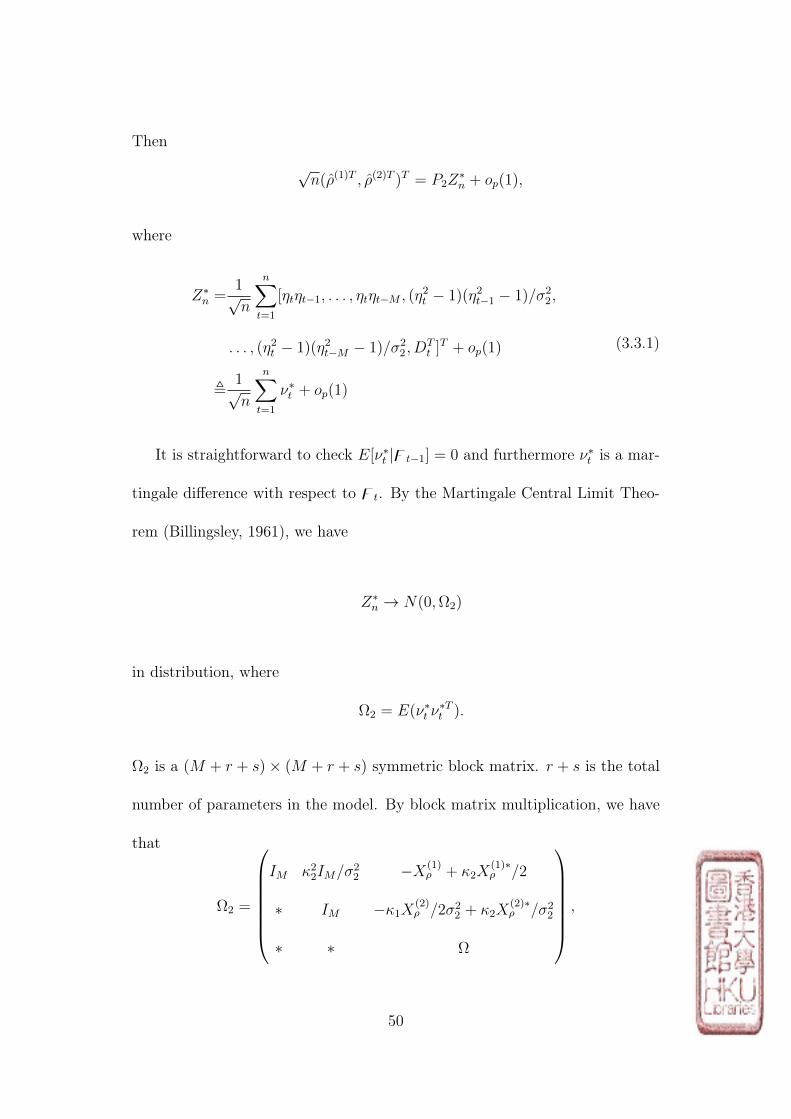
,1√n
n∑t=1
ν∗t + op(1)
(3.3.1)
It is straightforward to check E[ν∗t |zt−1] = 0 and furthermore ν∗t is a mar-
tingale difference with respect to zt. By the Martingale Central Limit Theo-
rem (Billingsley, 1961), we have
Z∗n → N(0,Ω2)
in distribution, where
Ω2 = E(ν∗t ν∗Tt ).
Ω2 is a (M + r + s)× (M + r + s) symmetric block matrix. r + s is the total
number of parameters in the model. By block matrix multiplication, we have
that
Ω2 =
IM κ22IM/σ
22 −X(1)
ρ + κ2X(1)∗ρ /2
∗ IM −κ1X(2)ρ /2σ2
2 + κ2X(2)∗ρ /σ2
2
∗ ∗ Ω
,
50
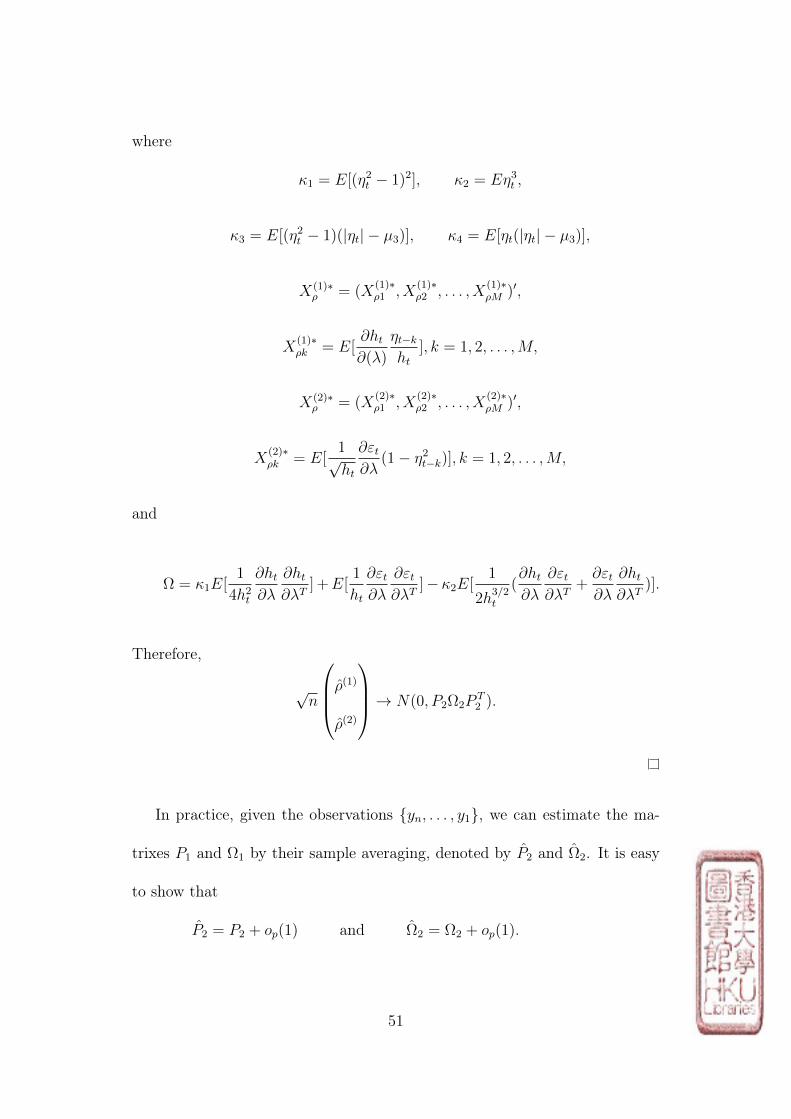
where
κ1 = E[(η2t − 1)2], κ2 = Eη3t ,
κ3 = E[(η2t − 1)(|ηt| − µ3)], κ4 = E[ηt(|ηt| − µ3)],
X(1)∗ρ = (X
(1)∗ρ1 , X
(1)∗ρ2 , . . . , X
(1)∗ρM )′,
X(1)∗ρk = E[
∂ht∂(λ)
ηt−kht
], k = 1, 2, . . . ,M,
X(2)∗ρ = (X
(2)∗ρ1 , X
(2)∗ρ2 , . . . , X
(2)∗ρM )′,
X(2)∗ρk = E[
1√ht
∂εt∂λ
(1− η2t−k)], k = 1, 2, . . . ,M,
and
Ω = κ1E[1
4h2t
∂ht∂λ
∂ht∂λT
] +E[1
ht
∂εt∂λ
∂εt∂λT
]−κ2E[1
2h3/2t
(∂ht∂λ
∂εt∂λT
+∂εt∂λ
∂ht∂λT
)].
Therefore,
√n
ρ(1)ρ(2)
→ N(0, P2Ω2PT2 ).
In practice, given the observations yn, . . . , y1, we can estimate the ma-
trixes P1 and Ω1 by their sample averaging, denoted by P2 and Ω2. It is easy
to show that
P2 = P2 + op(1) and Ω2 = Ω2 + op(1).
51

From the above theorem, we can design the following portmanteau statistic
Q∗2(2M) , n
ρ(1)ρ(2)
T
(P2Ω2PT2 )−1
ρ(1)ρ(2)
→d χ2(2M).
We use this portmanteau statistic for diagnostic checking of the proposed
general model with conational mean and variance fitted by the quasi-maximum
likelihood estimation method.
3.4 Simulation Study of Q∗1(2M) and Q∗2(2M)
In this section, we carry out some simulation experiments to study the perfor-
mance of two proposed portmanteau tests Q∗1(2M) and Q∗2(2M). We will also
compare the results with those individual portmanteau tests Q1(M) ∼ Q6(M).
In all experiments, we considered two different sample sizes, n = 200 and
n = 400. The number of replications is 1000 for each model and sample size
combination. For the sake of comparison, we choose the same null and alter-
native models as those in the simulation study in chapter 2:
We choose the null model H0:AR(1)− ARCH(1) as
52

yt = 0.5yt−1 + εt,
εt = ηt√ht,
ht = 0.01 + 0.4ε2t−1.
(3.4.1)
The following three alternative models are considered to investigate the
powers of each portmanteau tests. H1(1):AR(2)− ARCH(1):
yt = 0.5yt−1 + 0.2yt−2 + εt,
εt = ηt√ht,
ht = 0.01 + 0.4ε2t−1.
(3.4.2)
H1(2):AR(1)− ARCH(2):
yt = 0.5yt−1 + εt,
εt = ηt√ht,
ht = 0.01 + 0.4ε2t−1 + 0.3ε2t−2.
(3.4.3)
H1(3):AR(2)− ARCH(2):
yt = 0.5yt−1 + 0.1yt−2 + εt,
εt = ηt√ht,
ht = 0.01 + 0.4ε2t−1 + 0.2ε2t−2.
(3.4.4)
Note that the three alternative models represent the mean mis-specification,
53
variance mis-specification, mean and variance mis-specification jointly, respec-
tively.
We choose M = 6 as that in Wong and Ling (2005). The percentage of
rejections is based on the upper 5th percentile of the presumed χ2 distributions
with the degree of freedom 12.
Note that we have examined the sizes of portmanteau tests Q1(M) ∼
Q6(M) by simulation experiments in chapter 2. Therefore, we leave the cor-
responding entries blank in order to focus on our main objective in this chap-
ter, that is, examine the asymptotic distribution of mixed portmanteau test
Q∗1(2M) and compare its power with individual portmanteau tests Q1(M) ∼
Q6(M). The result is summarized in Table 3.1.
54

Based on the simulation results, we can make some conclusions.
1. The asymptotic results for the mixed portmanteau tests match the
theoretical values quite well for n as small as 200.
2. If the conditional mean is mis-specified, Q1(M) is slightly superior to
the mixed portmanteau test Q∗1(2M) and Q∗2(2M) in terms of the power, but
the latter ones have remarkable improvement in power compared with Q2(M),
Q3(M), Q5(M) and Q6(M).
3. If the conditional variance is mis-specified, Q3(M) Q2(M) are slightly
superior to the mixed portmanteau tests Q∗1(2M) and Q∗2(2M) in terms of the
power, but the latter ones have remarkable improvement in power compared
with Q1(M) and Q4(M).
4. The mixed portmanteau test Q∗1(2M) and Q∗2(2M) are feasible to detect
the mis-specification in both condition mean and conditional variance and
hence it is more robust.
5. In small sample size (n=200), Q∗2(2M) seems to be better than Q∗1(2M).
However, when the sample size become larger, we can clearly see that Q∗1(2M)
is superior to Q∗2(2M) in all three situations, that is, conditional mean mis-
specification, conditional variance mis-specification and both conditional mean
and variance mis-specification.
6. When the sample size becomes larger, the powers of all portmanteau
tests increase.
7. The distribution of ηt does not affect all the conclusions above.
55
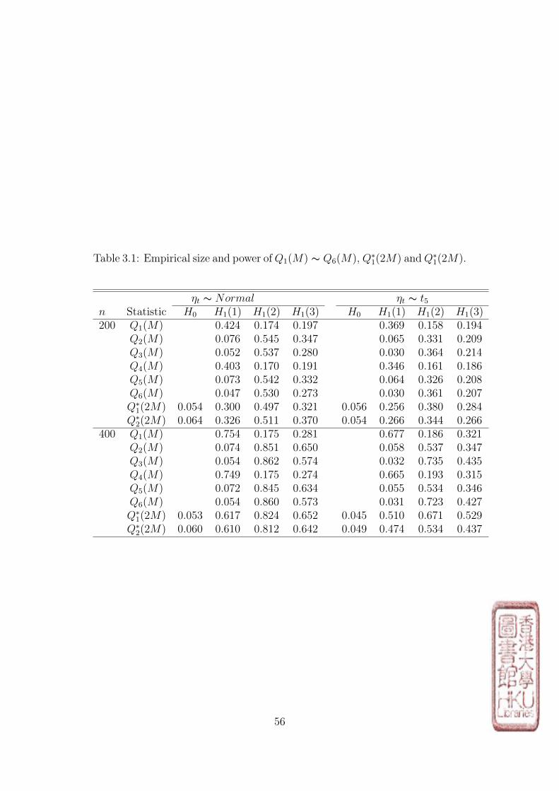
Table 3.1: Empirical size and power ofQ1(M) ∼ Q6(M), Q∗1(2M) andQ∗1(2M).
ηt ∼ Normal ηt ∼ t5n Statistic H0 H1(1) H1(2) H1(3) H0 H1(1) H1(2) H1(3)200 Q1(M) 0.424 0.174 0.197 0.369 0.158 0.194
Q2(M) 0.076 0.545 0.347 0.065 0.331 0.209Q3(M) 0.052 0.537 0.280 0.030 0.364 0.214Q4(M) 0.403 0.170 0.191 0.346 0.161 0.186Q5(M) 0.073 0.542 0.332 0.064 0.326 0.208Q6(M) 0.047 0.530 0.273 0.030 0.361 0.207Q∗1(2M) 0.054 0.300 0.497 0.321 0.056 0.256 0.380 0.284Q∗2(2M) 0.064 0.326 0.511 0.370 0.054 0.266 0.344 0.266
400 Q1(M) 0.754 0.175 0.281 0.677 0.186 0.321Q2(M) 0.074 0.851 0.650 0.058 0.537 0.347Q3(M) 0.054 0.862 0.574 0.032 0.735 0.435Q4(M) 0.749 0.175 0.274 0.665 0.193 0.315Q5(M) 0.072 0.845 0.634 0.055 0.534 0.346Q6(M) 0.054 0.860 0.573 0.031 0.723 0.427Q∗1(2M) 0.053 0.617 0.824 0.652 0.045 0.510 0.671 0.529Q∗2(2M) 0.060 0.610 0.812 0.642 0.049 0.474 0.534 0.437
56

Chapter 4
An Illustrative Example
In this section, we conduct a real data analysis to illustrate how to use these
tests, both individuals tests and mixed tests, to check whether the proposed
model is adequate. We also use this real data example to indicate that our
individual portmanteau tests are superior to the existing tests for this type of
models.
The data set we use in this section is the monthly log returns of IBM stock
based on the closing price. There is a total of 996 observations from January
1926 to December 2008. The returns are defined as
Yt = 100(logXt − logXt−1),
where Xt is the closing price at time t.
The reason why we choose the monthly return instead of the daily return
57
is that the daily returns tend to be distributed with zero mean based on the
efficient market theory. If that is the case, our model would degenerate to a
pure conditional heteroskedasticity model, such as ARCH and GARCHmodels.
The mean and standard deviation of this monthly log return series is equal
to 1.0891 and 7.0333 respectively. It seems that the mean is significantly
nonzero. The t test further confirms our observation with p − V alue 1.192 ×
10−6. We set M to be 10 in this section. Note that the theoretical chi-square
statistics with degree of freedom 10 and 20 are χ2(10) = 18.3070 and χ2(20) =
31.4104, respectively, when the significance level is 0.05.
First we model a GARCH(1,1) model. We clearly know the conditional
mean is mis-specified due to the previous argument. Our individual portman-
teau tests Q1(M) and Q4(M) with values 33.2376 and 26.8522 respectively,
and mixed portmanteau tests Q∗1(2M) and Q∗2(2M) with values 37.6950 and
39.8640 respectively, can correctly identify the mis-specification in the condi-
tional mean equation. However, the built-in portmanteau tests based on the
output of garchFit function in fGarch package of R software can not identify
the mis-specification in the conditional mean. Specifically, for the Ljung-Box
Test based on residual autocorrelation functions, when M is equal to 10 the
test statistic is 15.2719 with p− V alue 0.1225; when M is equal to 15 the test
statistic is 20.3862 with p−V alue 0.1576; when M is equal to 20 the test statis-
tic is 27.1920 with p − V alue 0.1299. For the conditional variance equation,
both the built-in tests and our individual tests Q2(M), Q3(M), Q5(M) and
58

Q6(M) indicate the model is adequate in modeling the heteroskedasticity, but
our tests are more sensitive, supported by the fact that Q2(M)=5.8221 and
Q5(M)=5.8935 are larger than 5.0273, which is the value of the Ljung-Box
test statistics with M=10.
Therefore, we can see that our individual portmanteau tests are superior
to existing tests for this type of model.
Next, we illustrate how to use these individual tests and mixed tests to
pick up an adequate model. Note that we set M to be 10 in the following
discussion.
We consider four models to fit the monthly log return seris Yt:
AR(3)− ARCH(4), AR(3)−GARCH(1, 1),
µ− AR(1)− ARCH(4), µ− AR(1)−GARCH(1, 1).
The fitted Model 1 is AR(3)− ARCH(4)
yt = 0.1103yt−1 + 0.0411yt−2 + 0.0538yt−3 + εt,
εt = ηt√ht,
ht = 26.1907 + 0.1437ε2t−1 + 0.0919ε2t−2 + 0.1372ε2t−3 + 0.1241ε2t−4,
where Q1(M) = 17.1869, Q2(M) = 21.1163, Q3(M) = 23.8432, Q4(M) =
17.5826, Q5(M) = 21.4392, Q6(M) = 25.3961, Q∗1(2M) = 42.5865 andQ∗2(2M) =
59

38.9472. Q1(M) and Q4(M), though don’t exceed the theoretical chi-squared
statistic value with 10 degrees of freedom at the 0.05 significance level, but
are very close to it. That indicates the model is inadequate in modeling the
conditional mean equation. The value of Q2(M), Q3(M), Q5(M) and Q6(M)
indicate the model is inadequate in modeling the conditional variance equation
either. The mixed tests Q∗1(2M) and Q∗2(2M) indicate the model is inadequate
as a whole.
The fitted Model 2 is AR(3)−GARCH(1, 1):
yt = 0.1054yt−1 + 0.0427yt−2 + 0.0452yt−3 + εt,
εt = ηt√ht,
ht = 3.0584 + 0.1054ε2t−1 + 0.8336ht−1,
(4.0.1)
where Q2(M) = 5.5455, Q3(M) = 5.1630, Q4(M) = 21.1470, Q5(M) = 5.6136,
Q6(M) = 5.1987, Q∗1(2M) = 25.3672 and Q∗2(2M) = 27.7269. The values
of Q1(M) and Q4(M) indicate the mis-specification in the conditional mean
equation. The values of Q2(M), Q3(M), Q5(M) and Q6(M) indicate that the
model is adequate in modeling the conditional variance equation. Q∗1(2M) and
Q∗2(2M), though don’t exceed the theoretical chi-squared statistic value with
20 degrees of freedom at the 0.05 significance level, but are very close to it.
That indicates that the model is inadequate as a whole.
60
The fitted Model 3 is µ− AR(1)− ARCH(4):
yt = 1.2058 + 0.0750yt−1 + εt,
εt = ηt√ht,
ht = 24.6607 + 0.1440ε2t−1 + 0.1122ε2t−2 + 0.1496ε2t−3 + 0.1177ε2t−4,
(4.0.2)
where Q1(M) = 10.9531, Q2(M) = 17.2460, Q3(M) = 21.9713, Q4(M) =
11.0132, Q5(M) = 17.4227, Q6(M) = 23.2969, Q∗1(2M) = 33.4795 andQ∗2(2M) =
28.5613. The values of Q1(M) and Q4(M) indicate that the model is adequate
in modeling the conditional mean equation. The values of Q3(M) and Q6(M)
indicate the conditional variance equation is mis-specified. Q2(M) and Q5(M),
though don’t exceed the theoretical chi-squared statistic value with 10 degrees
of freedom at the 0.05 significance level, but are very close to it. That indi-
cates the model is inadequate in modeling the conditional variance. Similarly,
Q∗1(2M) rejects the model and Q∗2(2M), which is close to the theoretical chi-
squared statistic value at the 0.05 significance level though it does not exceed
it, indicate the model is inadequate in modeling the conditional variance. The
result here is also consistent with our simulation results in Chapter 2 and Chap-
ter 3, in which we have stated that the portmanteau tests using the absolute
residual autocorrelation functions are more sensitive to the mis-specification in
the conditional variance than that using the squared residual autocorrelation
functions.
61
The fitted Model 4 is µ− AR(1)−GARCH(1, 1):
yt = 1.1328 + 0.0818yt−1 + εt,
εt = ηt√ht,
ht = 3.2434 + 0.1118ε2t−1 + 0.8222ht−1,
(4.0.3)
where Q1(M) = 9.9210, Q2(M) = 4.4080, Q3(M) = 4.0323, Q4(M) = 10.0892,
Q5(M) = 4.4999, Q6(M) = 4.0658, Q∗1(2M) = 13.9269 and Q∗2(2M) =
14.2265. All the statistics’ values are largely smaller than the correspond-
ing theoretical chi-squared statistic value with 10 and 20 degrees of freedom at
the 0.05 significance level. That indicates the model is adequate in all aspects.
Further, we make some arguments based on the above results.
1. If we focus on the outputs of Model 1 or 2, both in which the conditional
variance is mis-specified, we can find Q4(M), Q5(M) and Q6(M) are large than
their counterparts Q1(M), Q2(M) and Q3(M), respectively. This result will
stay the same no matter the conditional mean equation is correctly specified
or not. However, when the conditional variance equation is correctly specified,
we can find Q4(M), Q5(M) and Q6(M) are very close to their counterparts,
Q1(M), Q2(M) and Q3(M), respectively, from the outputs of Model 2 and
Model 4. The results convince us the usefulness of portmanteau tests based
on partial autocorrelation functions.
2. Another fact is that the mixed test Q∗1(2M) is sensitive to the mis-
62

specification in the conditional variance based on the outputs of Model 1 and
Model 3 and hence superior to the mixed test Q∗2(2M). This result is consistent
with the simulation study in Chapter 3.
3. When the model is correctly specified, the mixed tests is very close to
a direct summation of the two corresponding individual tests, see the outputs
of Model 4. Therefore, sometime mixed tests can be simplified to a direct
summation form of two individual tests. However, this fact may not be true
when the model is mis-specified, see the outputs of Model 1, Model 2 and
Model 3. Hence, if possible, we still recommend to use the complete form of
the mixed tests in practice.
4. We need to point out that both individual tests and mixed tests are
indispensable. For example, in Model 2, the mixed tests don’t exceed the
theoretical chi-squared statistic value, though very close to. It drives us to
doubt the adequacy of the model. At the same time, the individual tests clearly
show the model is inadequate and hence gives us more confidence to reject the
model. On the other hand, note that the theoretical chi-square statistics with
degree of freedom 10 and 20 are χ2(10) = 18.3070 and χ2(20) = 31.4104. From
the last argument, we may encounter the case in practice when both individual
tests don’t exceed the theoretical value 18.3070 but the mixed test based on
these two individual test does.
From this example, we can see that our individual tests are superior than
the existing tests built in popular statistical software. This individual tests,
63

together with the mixed portmanteau test would be a useful tool in checking
the adequacy of nonlinear time series models with conditional mean and condi-
tional heteroskedasticity. In the real application, especially the financial time
series, in which modeling the conditional heteroskedasticity may be more im-
portant than the conditional mean, we recommend to useQ∗1(2M),Q4(M),Q5(M)
and Q6(M) as a diagnostic checking package for this type of models.
64
Chapter 5
Conclusion
In this thesis, we choose a very general time series model that can represent
a wide class of the conditional mean and the conditional variance models.
We investigate the asymptotic distribution of some forms of residuals auto-
correlation functions from the general time series models fitted by Gaussian
quasi-maximum likelihood estimation method. Based on this we devise some
individual portmanteau tests using residual autocorrelation functions. We at-
tach equal importance to the residual partial autocorrelation functions as well,
which didn’t obtain much attention before in literature. By investigating the
relationship between residual autocorrelation functions and partial autocorre-
lation functions, we devise some individual portmanteau tests based on residual
partial autocorrelation functions. We illustrate the corresponding powerful-
ness of those individual portmanteau tests in detecting mis-specification in
65

the conditional mean and the conditional variance respectively by simulation
experiments. Based on findings from simulation experiments, we devise two
mixed portmanteau tests aiming at detecting the mis-specification in both the
conditional mean and the conditional variance.
First we summarize the findings about the comparison between the indi-
vidual tests and mixed tests. In different cases of mis-specification, some tests
are more powerful than others. When the conditional mean is mis-specified,
Q1(M) is slightly superior to the mixed test Q∗1(2M) and Q∗2(2M) in terms of
the power, but the latter ones have remarkable improvement in power com-
pared withQ2(M), Q3(M), Q5(M) andQ6(M). When the conditional variance
is mis-specified, Q3(M) and Q2(M) are slightly superior to the mixed port-
manteau tests Q∗1(2M) and Q∗2(2M) in terms of the power, but the latter ones
have remarkable improvement in power compared with Q1(M) and Q4(M).
When both the condition mean and conditional variance are mis-specified,
only mixed tests Q∗1(2M) and Q∗2(2M) are trustworthy. In such situation,
Q1(M) and Q4(M) work unsatisfactorily, while Q2(M), Q3(M), Q5(M) and
Q6(M) totally lack power.
Then we focus our attention to the residual partial autocorrelation func-
tions. We find that the values of individual tests based on partial autocorrela-
tion functions Q4(M), Q5(M) and Q6(M) are very close to their counterparts
Q1(M), Q2(M) and Q3(M) based on residual autocorrelation functions. How-
ever, when the conditional variance is mis-specified, we can findQ4(M), Q5(M)
66

and Q6(M) are large than their counterparts Q1(M), Q2(M) and Q3(M), re-
spectively. This result will stay the same no matter the conditional mean
equation is correctly specified or not. In addition, when the conditional vari-
ance equation is correctly specified, we can find Q4(M), Q5(M) and Q6(M) are
very close to their counterparts, Q1(M), Q2(M) and Q3(M), respectively. The
results convince us the usefulness of portmanteau tests based on partial auto-
correlation functions, especially when the conditional variance is mis-specified.
Regarding the comparison between the mixed tests Q∗1(2M) and Q∗2(2M),
we find that Q∗1(2M) is sensitive to the mis-specification in the conditional
variance and hence superior to the mixed test Q∗2(2M). We also find that
when sample size is large, Q∗1(2M) turns out to be a better one in terms of the
power.
We need to point out that both individual tests and mixed tests are in-
dispensable. In the real data example, it happens that the mixed tests don’t
exceed the theoretical chi-squared statistic value, though very close to. It
drives us to doubt the adequacy of the model. At the same time, the indi-
vidual tests clearly show the model is inadequate and hence gives us more
confidence to reject the model. On the other hand, as we point in the real
data example, we may encounter the case in practice when both individual
tests don’t exceed the theoretical value but the mixed test based on these two
individual test does.
There are also some other advantages of our tests. For example, the asymp-
67

totic results for all the individual and mixed portmanteau tests match the the-
oretical values quite well for n as small as 200. The distribution of ηt does
not affect all the conclusions. In fact, in the real data example, the distribu-
tion of ηt is totally unknown. Also, our individual tests are better than the
built-in diagnostic tests for the same type of models in the R software. Besides,
since the time series model based on which we devised portmanteau tests is
very general, we expect the extensive applications of our tests in practice.
In the real application, especially the financial time series, in which mod-
eling the conditional heteroskedasticity may be more important than the con-
ditional mean, we recommend to use Q∗1(2M),Q4(M) and Q6(M) as a diag-
nostic checking package for this type of models. If Q4(M) is significant but
Q6(M) and Q∗1(2M) are insignificant, we are given strong evidence that the
mis-specification only happens in the conditional mean. If Q6(M) is signifi-
cant but Q4(M) and Q∗1(2M) are insignificant, it is very likely that the mis-
specification only happens in the conditional variance rather than the condi-
tional mean. In sum, the package of the mixed portmanteau test Q∗1(2M) and
two individual portmanteau tests Q4(M) and Q6(M) will benefit our judge-
ment on whether the model inadequacy comes from the conditional mean or
the conditional variance.
68

Bibliography
Billingsley, P. (1961), “The Linderberg-Levy Theorem for Martingales.” Pro-
ceedings of the American Mathematical Society,, 12, 788–792.
Bollerslev, T. (1986), “Generalized autoregression conditional heteroscedastic-
ity,” Journal of Econometrics, 31, 307–327.
Box, G. E. P. and Pierce, D. A. (1970), “Distribution of the residual autocor-
relations in autoregressive integrated moving average time series models,”
Journal of the American Statistical Association, 65, 1509–1526.
Engle, R. F. (1982), “Autoregression conditional heteroscedasticity with esti-
mates of the variance of U.K. inflation,” Econometrica, 50, 987–1008.
Hall, P. and Yao, Q. (2003), “Inference in ARCH and GARCH models with
heavy-tailed errors,” Econometrica, 71, 285–317.
Lehmann, E. L. (1998), “Elements of Large-Sample Theory.” New York
Springer.
Li, G. and Li, W. K. (2005), “Diagnostic checking for time series models with
69
conditional heteroscedasticity estimated by the least absolute deviation ap-
proach,” Biometrika, 92, 691–701.
— (2008), “Least absolute deviation estimation for fractionally integrated
autoregressive moving average time series models with conditional het-
eroscedasticity,” Biometrika, 95, 399–414.
Li, W. K. and Mak, T. K. (1994), “On the squared residual autocorrelations in
nonlinear time series with conditional heteroskedasticity,” Journal of Time
Series Analysis, 15, 627–636.
Ljung, G. M. and Box, G. E. P. (1978), “On a measure of lack of fit in time
series models,” Biometrika, 65, 297–303.
McLeod, A. I. and Li, W. K. (1983), “Diagnostic checking ARMA time series
models using squared residual autocorrelations,” Journal of Time Series
Analysis, 4, 269–273.
Miller, R. B. (1979), “Book review on An introduction to Bilinear Time Series
Models,” Journal of the American Statistical Association, 74, 927.
Monti, A. C. (1994), “A proposal for a residual autocorrelation test in linear
models,” Biometrika, 81, 776–780.
Peng, L. and Yao, Q. (2003), “Least absolute deviations estimation for ARCH
and GARCH models,” Biometrika, 90, 967–975.
70

Weiss, A. (1986), “Asymptotic theory for ARCH models: estimation and test-
ing,” Econometric Theory, 2, 107–131.
Wong, H. and Ling, S. (2005), “Mixed portmanteau tests for time-series mod-
els,” Journal of Time Series Analysis, 26, 569–579.
71