FullText (31)
146
Title 3D reconstruction of coronary artery and brain tumor from 2D medical images Author(s) Law, Kwok-wai, Albert.; 羅國偉. Citation Issued Date 2004 URL http://hdl.handle.net/10722/51497 Rights The author retains all proprietary rights, (such as patent rights) and the right to use in future works.
description
thes
Transcript of FullText (31)
Title 3D reconstruction of coronary artery and brain tumor from 2Dmedical images
Author(s) Law, Kwok-wai, Albert.; 羅國偉.
Citation
Issued Date 2004
URL http://hdl.handle.net/10722/51497
Rights The author retains all proprietary rights, (such as patent rights)and the right to use in future works.

3D Reconstruction of Coronary Artery and Brain Tumor
from 2D Medical Images
Law Kwok Wai Albert
B.Eng. H.K.U.
A thesis submitted in partial fulfillment of the requirements for
the Degree of Doctor of Philosophy
at The University of Hong Kong
June 2004
Declaration
I declare that this thesis represents my own work, except where due acknowledgement
is made, and that it has not been previously included in a thesis, dissertation or report
submitted to this University or to any other institution for a degree, diploma or other
qualification.
Signed
Law Kwok Wai Albert
Acknowledgements
I wish to express my sincere gratitude to my supervisors, Prof. Francis H. Y .
Chan and Dr. F. K . Lam, for their continual advice, guidance, and encouragement
throughout my postgraduate study. I would like to thank Prof. Paul W. F. Poon,
Department of Physiology,National Cheng Kung University, Taiwan, and Prof.
Morton H. Friedman, Department of Biomedical Engineering, Duke University, USA,
for their visiting invitations. I would like to express my thanks to Prof. K. Y. Lam,
Department of Pathology, James Cook University, Australia, Dr. H. Zhu,Department
of Biomedical Engineering, Duke University, USA, Dr. Brent C. B. Chan and Dr. P.
P. lu, Department of Radiology, Kwong Wah Hospital, Hong Kong for their valuable
suggestions to my research work. Thanks should also be given to Dr. Chunqi Chang,
Dr. George S. K. Fung, Dr. Weichao Xu, Miss M. M. Au, Miss Jiyun Ren, Miss
Teresa K. W. Wong, Mr. Neil S. K. Kwan, Mr. Gary C. C. Leung, Mr. K. H. Ting,
and Mr. Jianchao Yao in our research group for their assistance and help.
Finally, financial support from Postgraduate Studentship, Swire Scholarship,
Hung Hing Ying Scholarship, Taipei Trade Centre Exchange Scheme, CRCG
Conference Grant, and Swire Travel Grant is gratefully acknowledged.

Abstract of thesis entitled
3D Reconstruction of Coronary Artery and Brain Tumor
from 2D Medical Images
Submitted by
Law Kwok Wai Albert
for the degree of Doctor of Philosophy
at The University of Hong Kong
in June 2004
The technique of 3D medical image reconstruction plays a useful role in
medical diagnosis and prognosis, as it enables 3D biological objects to be derived
from 2D medical images such as X-ray and M R images. There are two main types of
3D reconstruction: the multiview approach and the multislice approach. The
multiview approach reconstructs the 3D volume using the 2D projection images from
different view angles. The multislice approach reconstructs the 3D volume by
stacking the spatially contiguous and aligned slices on top of each other.
In this study, two novel methods were developed for the 3D reconstruction of
2D images in medical applications, one using the multiview approach and the other
using the multislice approach. They were applied to reconstruct 3D representation of a
coronary artery from biplane angiograms and of a brain tumor from multislice M R
images.
In order to reconstruct 3D representation of coronary arteries from biplane
angiograms, a pair of 2D projection images of a coronary artery was captured from
different view angles. A front propagation algorithm was used to reconstruct the
coronary artery pathways and centerlines in 3D space. The reconstruction was
controlled by the combined image information from two 2D projection images. After
front propagation, the vessel diameter was estimated along the extracted 3D
centerlines based on the reconstructed 3D coronary artery pathways. The 3D
smoothed coronary artery pathways were reconstructed using the position and
diameter at each point of the vessel centerlines.
In order to reconstruct 3D representation of brain tumors from multislice M R
images, multislice M R images of a brain tumor were captured at a fixed distance
between each other. The shape and position of tumor in one slice was assumed to be
similar to that of neighboring slices. Using this correlation between consecutive
images, the initial plan applied to each slice was obtained from the resulting boundary
of the previous slice. The tumor boundary was located by a two-step method,
involving region deformation followed by contour deformation, with a fairly rough
initial plan. The advantage of this method is that only one coarse manual initial plan is
required for the whole series of M R image slices. The tumor was then reconstructed
in 3D space using the located tumor boundary at each slice of the M R image series.
The proposed 3D reconstruction methods may also be used in multiview
multislice 3D reconstructions in other medical applications. They can be applied for
the 3D reconstruction of blood vessels and tumors in other parts of the body. They can

also be used for the reconstruction of 3D representation of bones, of organs such as
the heart, lungs and brain, and even of biological cells.
Contents
Declaration
Acknowledgements
Contents
List of Figures
List of Tables
Author's Publications
Chapter 1 Introduction
1.1 Preamble
1.2 Medical Imaging
1.2.1 X-Ray
1.2.2 Computed Tomography
1.2.3 Magnetic Resonance Imaging
1.3 Medical Image Processing
1.3.1 Boundary Detection
1.3.2 Segmentation
1.3.3 Tracking
1.3.4 3D Reconstruction
1.4 3D Reconstruction from 2D Medical Images
1.4.1 Multiview Approach
1.4.2 Multislice Approach
1.5 3D Reconstruction Technique in Medical Imaging 1-13
1.5.1 A Typical Deformable Model --- “Snake” 1-14
1.5.2 Variations in Deformable Models 1-15
1.6 Clinical Applications of 3D Reconstruction of Medical Images 1-18
1.7 Motivations 1-19
1.8 Research Goals and Objectives 1-20
1.9 Contributions 1 -21
1.10 Thesis Organization 1 -22
1.11 References 1-23
Chapter 2 3D Reconstruction of Coronary Artery
from Biplane Angiograms 2-1
2.1 Preamble 2-1
2.2 Introduction 2-1
2.3 Related Research 2-4
2.3.1 Segmentation 2-5
2.3.2 3D Reconstruction 2-7
2.4 Methodology
2.4.1 Image Acquisition and Preprocessing 2_ 10
2.4.2 A 3D Vessel Response Measure 2_ 11
2.4.3 Front Propagation 2-13
2.4.4 Reconstruction of the 3D Coronary Artery 2-15
2.5 Validation 2一18
2.6 Results 2-19
iv
2.6.1 Comparisons of Fixed Thresholding and Adaptive Thresholding 2-19
2.6.2 Results of Validation with the Coronary Arterial Phantom 2-22
2.6.3 Results of Coronary Artery Reconstruction 2-26
2.7 Discussions 2-34
2.8 Summary 2-36
2.9 References 2-37
Chapter 3 3D Reconstruction of Brain Tumor
from Multislice MR Images 3-1
3.1 Preamble 3-1
3.2 Introduction 3-1
3.3 Related Research 3-4
3.3.1 Boundary Detection 3-5
3.4 Methodology 3-7
3.4.1 Region Deformation 3-8
3.4.2 Contour Deformation 3-10
3.5 Analysis of Results 3-11
3.6 Results 3-11
3.6.1 Comparisons of Proposed Model and Deformable Region Model 3-11
3.6.2 Tolerance of the Two-step Method 3-14
3.6.3 Comparisons of GVF Snake and Two-step Method 3-16
3.6.4 Processing of M R Image Sets 3-18
3.7 Discussions
3.8 Summary 3-34

3.9 References 3-34
Chapter 4 Conclusions and Future Works 4-1
4.1 Conclusions 4-1
4.2 Future Works 4-2
Appendix A-l
v i

List of Figures
Fig. 1.1 The medical object scanned at various view angles. 1-11
Fig. 1.2 The medical object scanned at various levels. 1 -11
Fig. 2.1 Block diagram of the coronary artery 3D reconstruction approach. 2-10
Fig. 2.2 A coronary arterial phantom. 2-18
Fig. 2.3 (a) L A O projection image, (b) Segmentation result by fixed
thresholding method, (c) Segmentation result by adaptive
thresholding method. 2-20
Fig. 2.4 (a) RAO projection image, (b) Segmentation result by fixed
thresholding method, (c) Segmentation result by adaptive
thresholding method. 2-21
Fig. 2.5 (a) LAO and (b) RAO projection pairs of a coronary arterial
phantom. 2-23
Fig. 2.6 Segmentation results of the (a) LAO and (b) RAO projection
images. 2-23
Fig. 2.7 The 3D reconstructed centerline of coronary arterial phantom
projected back to the ⑷ LAO and (b) RAO projection images. 2-24
Fig. 2.8 (a) LAO and (b) RAO projection pairs of a coronary arterial
phantom. 2-25
Fig. 2.9 Segmentation results of the (a) LAO and (b) RAO projection
images. 2-25
Fig. 2.10 The 3D reconstructed centerline of coronary arterial phantom
projected back to the (a) LAO and (b) RAO projection images. 2-26
vii
Hg. 2.11 (a) LAO and (b) RAO projection pairs of a right coronary artery. 2-27
Fig. 2.12 Segmentation results of adaptive thresholding applied to the (a)
LAO and (b) RAO projection images. 2-28
Fig. 2.13 The 3D reconstructed coronary artery centerline projected back to
the (a) LAO and (b) RAO projection images. 2-28
Fig. 2.14 The 3D coronary artery pathway at different view angles. 2-29
Fig. 2.15 The diameter of coronary artery plotted against the position along
vessel centerline. 2-30
Fig. 2.16 (a) L A O and (b) RAO projection pairs of a left coronary artery. 2-31
Fig. 2.17 Segmentation results of adaptive thresholding applied to the (a)
L A O and (b) RAO projection images. 2-31
Fig. 2.18 The 3D reconstructed coronary artery centerline projected back to
the (a) LAO and (b) RAO projection images. 2-32
Fig. 2.19 The 3D coronary artery pathway at different view angles. 2-33
Fig. 2.20 The diameter of coronary artery plotted against the position along
vessel centerline. 2-34
Fig. 3.1 Block diagram of the brain tumor 3D reconstruction approach. 3-8
Fig. 3.2 (a) Initial plan outside the brain tumor, (b) Tumor boundary result
from initial plan shown in (a) for 15. 3-13
Fig. 3.3 (a) Initial plan inside the brain tumor, (b) Tumor boundary result
from initial plan shown in (a) foTk= 15. 3-13
Fig. 3.4 (a) Initial plan of tumor boundary, (b) Tumor boundary result from
initial plan shown in (a), (c) Tolerable radius range of circular initial
plans of the two-step method, (d) Tolerable radius range of circular
initial plans of the fast snake method. 3-15
Vlll
Fig. 3.5 (a) Initial plan outside brain tumor, (b) Tumor boundary result by
GVF snake, (c) Tumor boundary result by two-step method. 3-17
Fig. 3.6 (a) Initial plan inside brain tumor, (b) Tumor boundary result by
GVF snake, (c) Tumor boundary result by two-step method. 3-18
Fig. 3.7 Selected image slices from a M R image set containing a brain
tumor. 3-21
Fig. 3.8 Extracted tumor boundaries, superimposed on the original image
slices from the M R image set in Fig. 3.7. 3-22
Fig. 3.9 The 3D reconstructed tumor at different view angles. 3-23
Fig. 3.10 Selected image slices from another M R image set containing a brain
tumor. 3-26
Fig. 3.11 Extracted tumor boundaries, superimposed on the original image
slices from the MR image set in Fig. 3.10. 3-28
Fig. 3.12 The 3D reconstructed tumor at different view angles. 3-29
ix

List of Tables
Table 2.1 Results of validation with the coronary arterial phantom. 2-26
Table 3.1 The computation time required for different values of k in the brain
tumor boundary extraction using two kinds of initial plans. 3-14
Author、Publications
[1] A. K. W. Law, F. K. Lam, K. Y. Lam, F. H. Y. Chan, T. K. W. Wong,and J. L.
S. Poon, "Computer-based counting for MIB-1 stained nuclei in esophageal
cancer," in Proceedings of the Annual Conference of Engineering and the
Physical Sciences in Medicine, Newcastle, Australia, 2000, pp. 82.
[2] A. K. W. Law, H. Zhu, B. C. B. Chan,P. P. Iu3 F. K. Lam, and F. H. Y. Chan,
"Semi-automatic tumor boundary detection in MR image sequences," in
Proceedings of2001 International Symposium on Intelligent Multimedia , Video
and Speech Processing, Hong Kong, 2001,pp. 28-31.
[3] A. K. W. Law, H. Zhu, F. K. Lam, F. H. Y. Chan, B. C. B. Chan, and P. P. Iu,
“Tumor boundary extraction in multislice MR brain images using region and
contour deformation," in Proceedings of International Workshop on Medical
Imaging and Augmented Reality, Hong Kong,2001, pp. 183-187.
[4] A. K. W. Law,F. K. Lam, K. Y. Lam, F. H. Y. Chan,and D. S. K. Chan,
“Image-based method for estimating the aspect ratio of thyroid cancer cells,” in
Proceedings of the Annual Conference of Engineering and the Physical
Sciences in Medicine and Asia Pacific Conference on Biomedical Engineering,
Fremantle, Australia, 2001,pp. 173.
[5] A. K. W. Law, F. K. Lam, and F. H. Y. Chan, “A fast deformable region model
for brain tumor boundary extraction," in Proceedings of the Second Joint
EMBS/BMES Conference , Houston, USA,2002,pp. 1055-1056.
[6] A. K. W. Law, K. Y. Lam, F. K. Lam, T. K. W. Wong,J. L. S. Poon, and F. H.
Y. Chan,"Image analysis system for assessment of immunohistochemically
xi

stained proliferative marker (MIB-1) in oesophageal squamous cell carcinoma,”
Computer Methods and Programs in Biomedicine, vol. 70,pp. 37-45, 2003.
[7] A. K. W. Law, K. Y. Lam, F. K. Lam, M. M. Au, and F. H. Y. Chan, “A new
computer-based method for counting MIB-1 stained nuclei in esophageal
cancer," in Proceedings of World Congress on Medical Physics and Biomedical
Engineering, Sydney, Australia, 2003.
[8] A. K. W. Law, H. Zhu, and F. H. Y. Chan, “3D reconstruction of coronary
artery using biplane angiography," in Proceedings of the 25th Annual
International Conference of the IEEE Engineering in Medicine and Biology
Society, Cancun, Mexico,2003,pp. 533-536.
xii
Chapter 1 Introduction
Chapter 1
Introduction
1.1 Preamble
It is difficult to visualize the three dimensional (3D) geometry of anatomical
and histological structures from two dimensional (2D) medical images. Computerized
modeling of anatomical and histological structures has become very powerful for
displaying and visualizing complex three dimensional forms. Computer models not
only provide a way to visualize 3D complex structures from 2D medical images, but
also permit mathematical modeling of medical diagnosis and investigation. Prior to
the 1970,8, initial attempt was made to generate 3D models based on graphical
reconstruction. Outlines of histological structures were traced on opaque paper and
superimposed to provide a 3D model. Computerized applications of 3D modeling
began during the 1970fs. Structural edges were digitized and histological structures
were expressed as line reconstructions. However, surface information was not
sufficient in these reconstructions. Significant research effort was then made to
develop models in dealing with various 3D reconstruction problems,such as surface
modeling in 3D space. For the past decade, deformable models have raised much
interest and found a wide variety of applications in the fields of computer vision and
medical imaging. They have been used for pattern recognition,boundary tracking,
image registration, 3D reconstruction. Among them,surface representations,
1-1
Chapter 1 Introduction
boundary detection, and segmentation based on deformable models have been
developed to tackle different 3D reconstruction problems.
1.2 Medical Imaging
Medical imaging has undergone a phenomenal growth during the last century.
Rapid developments of powerful computers, advanced imaging systems, and digital
image processing techniques have contributed a lot to medical imaging. It has become
one of the most important parts in the fields of medicine and science. The use of
medical images is very common for medical diagnosis and scientific research in
clinics, hospitals, and research institutes.
Medical imaging is the interaction of anatomical and histological structures
with various forms of radiation as well as the development of appropriate technology
to extract clinically useful information from observations of this interaction [1]. Such
information is generally displayed in an image format. There are different types of
medical images. It can be ranged from a projection image, such as X-ray, to a
computer reconstructed image, such as computed tomography using X-rays and
magnetic resonance imaging using intense magnetic fields. Medical images can
provide various kinds of medical and biological information. Systems utilizing
projection images give anatomic information, while others utilizing radioisotopes
provide functional information [2]. If both anatomic and functional information are
required, technology has to be developed to merge these data for further research and
investigations.
The beginning of medical imaging can be regarded as Roentgen's discoveries
of X-rays in 1895 [3]. A beam of X-rays was directed through the patient onto a film.
The developed film provided a projection image as a direct representation of the X -
1-2
Chapter 1 Introduction
ray passage through the patient s body. It was used to visualise bones and other
structures within the living body. The wide application of X-ray systems in medicine
is because of their processing speed as well as the cost of system acquisition and
diagnostic procedure.
Contemporary medical imaging began in the 1970,s with the invention of
computed tomography (CT) [4]. The first X-ray CT device was developed by G. N.
Hounsfield in 1972 at EMI in England. It was based in part on the mathematical
methods developed by A. M. Cormack [5] a decade earlier. Mathematical methods
were used to reconstruct tomographic (cross sectional) images of the structure, if
enough projection data from different angles were obtained. The development of CT
revolutionized medical radiology that physicians could acquire high quality
tomographic images of inner structures of the body.
In 1972, the birth of X-ray CT, NMR (nuclear magnetic resonance) imaging
began to appear and was applied in medicine. It was commonly known as MRI
(magnetic resonance imaging). The phenomenon of NMR was discovered
independently by Felix Bloch and Edward Purcell. The work was extended to produce
NMR spectra by Richard R. Emst. Kumar et al. [6] made a major contribution to form
the basis of modem MRI in 1975. Comparing to X-ray CT, MRI is non-invasive and
has better image contrast. However, MRI is slow in speed and the deformation of
structure shape is larger.
While X-ray CT and MRI give anatomic information of structure, SPECT
(single photon emission computed tomography) and PET (positron emission
tomography) can provide the functional information by monitoring the physiological
functional processes of the inner organs [2]. Now, MRI is moving from static imaging
to dynamic imaging,so it can also study the physiological functional processes.
1-3
Chapter 1 Introduction
Ultrasound imaging [2] of the soft tissue within the body began in the early
1970 s. Technologies available were able to capture and display the echoes
backscattered by structures within the body as images, static compound images, and
real-time moving images. The systems could show organ motions and dimensions as
well as structural relations.
Apart from the above medical imaging modalities,infrared imaging, light
microscopic imaging,confocal microscopic imaging are common tools applied in
medicine and science. Details of some medical imaging modalities will be given as
follows.
1.2.1 X-Ray
Conventional X-ray radiography [7] generates anatomic images that are
shadowgrams based on the X-ray absorption. The X-rays, which are produced from
nearly a point source, are directed on the structure to be imaged. The X-rays emerging
from the anatomy are detected to form a 2D image,where each point in the image has
a brightness related to the intensity of the X-rays at that point. Image production
depends on the amounts of X-rays penetrating through the structure and the amounts
of X-rays absorbed by different parts of the structure. If the structure of interest does
not absorb X-rays differently from surrounding regions,image contrast may be
increased by introducing strong X-ray absorbers.
X-rays striking an object may either pass through unaffected or may undergo
an interaction. These interactions usually involve either the photoelectric effect
(where the X-ray is absorbed) or scattering (where the X-ray is deflected to the side
with a loss of energy). X-rays that have been scattered may undergo deflection
through a small angle and still reach the image detector; in this case they reduce
1-4

Chapter 1 Introduction
image contrast and thus degrade the image. This degradation can be reduced by
introducing an air gap between the structure and the image receptor or by using an
antiscatter grid.
Angiography [8] is a diagnostic and therapeutic modality concerned with
disease of the circulatory system such as vascular disease. Projection radiography
studies the vascular structure in which the vessel of interest is opacified by injection
of a radiopaque contrast agent. Contrast material is needed to opacify vascular
structures because the radiographic contrast of blood is essentially the same as that of
soft tissue. Serial radiographs of the contrast material flowing through the vessel are
then acquired. This examination is performed in an angiographic suite,a special
procedure laboratory, or a cardiac catheterization laboratory. Some cine angiographic
installations provide biplane imaging in which two independent imaging chains can
acquire orthogonal images of the injection sequence. The acquisition of multiple X«
ray projections may be required because of the eccentricity of coronary lesions and
the asymmetric nature of cardiac contraction abnormalities.
1.2.2 Computed Tomography
The development of computed tomography (CT) [4] revolutionised medical
radiology that physicians could obtain high quality tomographic images of inner
structures of the body. Computed tomographic images are reconstructed from a large
number of measurements of X-ray transmission through the patient, which is called
projection data. Projection data may be acquired in one of several possible geometries:
parallel-beam geometry, fan beam with multiple detectors,fan beam with rotating
detectors, fan beam with fixed detectors, and scanning electron beam [9]. The
resulting images are tomographic “maps” of the X-ray linear attenuation coefficient.
1-5
Chapter 1 Introduction
Both iterative and analytical estimations of the X-ray linear attenuation have been
used for transmission CT reconstruction. Iterative estimation was used in the first
commercially successful CT scanner [10]. It permits easy incorporation of physical
processes that cause deviations from the linearity. However, its practical usefulness is
limited. Analytical estimation or direct reconstruction used a nunierical approxirnation
of the inverse Radon transform [11].
1.23 Magnetic Resonance Imaging
MRI [12] scanners use the technique of nuclear magnetic resonance to induce
and detect a very weak radio frequency signal that is a manifestation of nuclear
magnetism. Nuclear magnetism refers to weak magnetic properties that are exhibited
by some materials as a consequence of the nuclear spin that is associated with their
atomic nuclei. The proton, which is the nucleus of the hydrogen atom,possesses a
nonzero nuclear spin and is an excellent source of NMR signals. The human body
contains enormous numbers of hydrogen atoms,especially in water and lipid
molecules. Although biologically significant NMR signals can be obtained from other
chemical elements in the body,such as phosphorous and sodium, the great majority of
clinical MRI studies utilize signals originating from protons that are present in the
water and lipid molecules within the body.
The patient to be imaged must be placed in an environment in which several
different magnetic fields can be simultaneously or sequentially applied to elicit the
desired NMR signal. Every MRI scanner utilizes a strong static field magnet in
conjunction with a set of coils and radiofrequency coils [13]. The gradients and the
radiofrequency components are switched on and off in a precisely timed pattern, or
pulse sequence. Different pulse sequences are used to extract different kinds of data
1-6

Chapter 1 Introduction
from the patient. M R images are characterized by excellent contrast between the
various forms of soft tissues within the body. MRI scanning is safe and can be
repeated very often when necessary without danger [14]. This is one of the major
advantages of MRI over X-ray and CT. Moreover, it is not necessary to add
radioactive tracer materials to the patient.
1.3 Medical Image Processing
The main objective of taking medical images is to extract useful medical and
biological information from them. Such information is important for medical and
scientific investigations. Information extraction from medical images usually involves
boundary detection, classification, counting, and size measurement. If it is done by
human only, the extracted information may be inaccurate and subjective. Moreover,it
is a tedious and time-consuming task. Digital image processing techniques can assist
human in the analysis of medical images. They can extract reliable, objective, and
accurate information quickly. Therefore, they have found contributions to this field.
This is known as medical image processing. Accurate and reliable processing results
are significant for medical diagnosis and scientific research. Since the development of
CT and MRI, 3D medical image processing [15] becomes vital and provides more
information in 3D space for diagnostic assessment and treatment of diseases. Medical
image processing techniques have been developed to work on 3D space beyond the
2D space. With the incorporation of time domain,they can be farther extended to 4D
space for motion tracking and monitoring. They contribute to accurate radiotherapy,
surgical planning and simulation.
Medical image processing techniques can accommodate the significant
variability of biological structures over time within an individual and across different
1-7

Chapter 1 Introduction
individuals. A priori knowledge from medical experts, such as radiologists and
pathologists, can be incorporated into the techniques. The applications of medical
image processing are very wide, covering every medical image modalities, various
parts of the body, and range of scale from the whole body to cellular components of
anatomic structures. There are different types of medical image processing techniques:
boundary detection, segmentation, tracking, and 3D reconstruction. Here some typical
examples wil l be given.
1.3.1 Boundary Detection
The application of medical image processing to cell recognition [16] has
drawn much attention in the field of cell biology. The cell recognition is often based
on the boundary detection techniques [17], [18]. Fok,Chan, and Chin [19] applied the
active contour model for the detection of nerve cell boundaries from electron-
micrographic images. A rough identification of all the axon centers was performed by
use of an elliptical Hough transform procedure. Boundaries of each axon were then
extracted based on active contour model. Physical properties of the axons were used
in an optimization scheme to guide the model to detect axon boundaries for accurate
sheath measurement. The number of nerve fibers (axons) in a nerve, the axon size,
and shape are important neuroanatomical features in understanding different aspects
of nerves in the brain. Potentially meaningful studies can be performed in objective,
reliable and accurate manner by applying medical image processing in cell
measurements.
1-8
Chapter 1 Introduction
1.3.2 Segmentation
The accurate segmentation of brain tissues [20], [21] has become more and
more important for visualisation, surgical planning, and intraoperative navigation. In
the latest research and investigation of this field, a 3D brain atlas is applied to match
to a newly obtained image volume for automatic segmentation, localization, and
identification of brain structures. In the brain atlas, curves or surfaces are used to
represent the anatomical knowledge of brain. The forces driving the surfaces towards
the desired locations in the image are functions of the image features and include the
prior brain information. Under these forces, curves or surfaces are deformed to
segment the whole 3D brain volume [22]-[24].
1.3.3 Tracking
Tracking is also an essential part in medical image processing for motion
monitoring. Heart wall motion tracking is a typical example. Heart wall motion has
important clinical implications for the assessment of viability in the heart wall. It is a
sensitive and useful indicator of heart disease such as ischemia. Heart wall motion can
be monitored and recorded in 2D image sequences such as echocardiography and
angiocardiography, or in 3D image sequences such as MRI. Various models [25]-[28]
were developed for the tracking of heart motion. The heart wall is located in the first
image of the sequence. Then the located boundaries or positions can be used as the
initial estimations to extract the heart wall in the next image. This process is repeated
for the whole image sequence. Finally,the motion of heart wall is detected over a
certain period of time.
1-9

Chapter 1 Introduction
1.3.4 3D Reconstruction
The technique of 3D reconstruction can be applied in different types of
medical objects. The application can cover the reconstruction of organs [29], [30],
biological structures [31], [32] and biological cells [33]. The 3D reconstructed
medical objects can be used to calculate a projection image with a reproducible angle
of view. It can provide important information regarding their changes in shape,
location and geometry. Selected anatomic features over a long time interval may be
compared, e.g. coronary artery stenosis or pulmonary opacity. The quantitative and
qualitative characteristics can be improved by integrating image information from one
imaging modality and another one. This technique is constructive and vital for the
diagnosis of diseases and radiation treatment planning.
1.4 3D Reconstruction from 2D Medical Images
As mentioned in the last section, 3D reconstruction is one of the most
important parts in medical image processing. Although medical objects can be
scanned and recorded in 3D data sets, the 3D anatomical information is often
converted to a 2D image, either in projection plane or cross sectional plane.
Ambiguities in shape,location and geometry may occur, resulting in interpretation
errors. Therefore,the reconstruction of 3D medical objects from 2D images is vital in
clinical applications as well as in medical and scientific researches. There are mainly
two types of 3D reconstruction: multiview approach and multislice approach. The
projection imaging modality,known as multiview approach,is to scan around the
medical object at various views as shown in Fig. 1.1. The 3D volume can be
reconstructed using the 2D projection images of the object from different view angles.
1-10
Chapter 1 Introduction
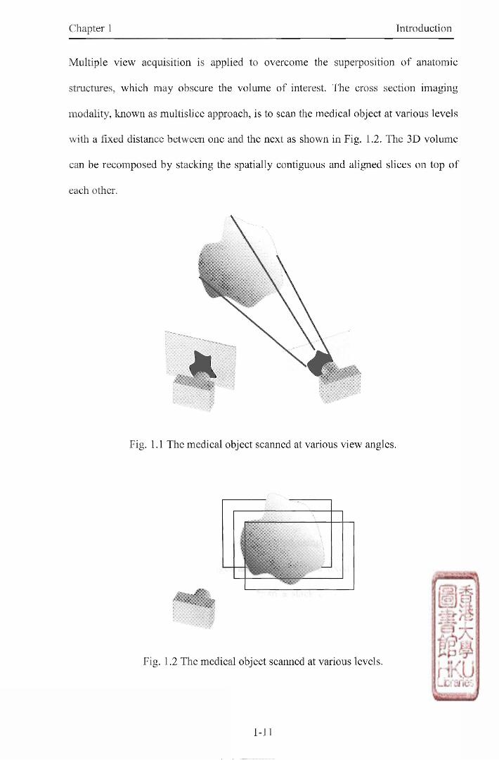
Multiple view acquisition is applied to overcome the superposition of anatomic
structures, which may obscure the volume of interest. The cross section imaging
modality, known as multislice approach, is to scan the medical object at various levels
with a fixed distance between one and the next as shown in Fig. 1.2. The 3D volume
can be recomposed by stacking the spatially contiguous and aligned slices on top of
each other.
Fig. 1.1 The medical object scanned at various view angles.
Fig. 1.2 The medical object scanned at various levels.
1-11
Chapter 1 Introduction
1.4.1 Multiview Approach
The 3D volume can be reconstructed using multiple 2D image projections of
the object at various view angles. There are some geometrical relationships between
the medical object and the 2D projection images. Calibration may be carried out to
determine these relationships in some cases [34]-[36], while it may not be required in
other cases [37]. In the coronary artery angiograms, a 3D Plexiglas cube, which
contains twelve radio-opaque markers in known position and orientation relation to
one another, and a Plexiglas board embedded with a gnd of radio-opaque balls are
imaged at the same geometry as it is used when capturing the artery images for the
calibration of the imaging system and correction of the pincushion distortion of the
projection images [38]. Effects of medical object overlap and foreshortening in
individual projection image can be mostly minimized by combining information from
various projection images. As only a very small number of projections, usually two or
three, is available, medical image processing techniques, such as image modelings,
are needed to incorporate the object information from different projection images for
the 3D reconstruction.
1.4.2 Multislice Approach
The 3D volume can also be reconstructed using a stack of 2D cross sectional
images. The cross sectional images are parallel with a fixed distance between each
other. The 3D data set can be built up from a stack of 2D cross sectional images.
Image rendering can be performed by surface or volume description. This includes
contour detection or segmentation [39],[40], piecewise linear approximation [41] and
triangulation [42] between portions of contours within adjacent cross sections. The
critical part is the contour detection or segmentation. The information regarding the
1-12
Chapter 1 Introduction
characteristics of organs and tissues is usually required in contour detection or
segmentation. Some attempts can be made to represent the 3D medical objects
through the combination of domain specific or a priori knowledge and contour
detection or segmentation methods. Accurate detected contours or segmented regions
are vital for the reconstruction of the 3D volume by image rendering. The best surface
approximation of the medical objects depends on the optimal selection of vertices on
the surface.
1.5 3D Reconstruction Technique in Medical Imaging
As described in the previous section, the 3D reconstruction usually involves
image modelings, surface or volume representations,contour detection,and
segmentation. Deformable model is one of the most important models for medical
image processing. It can be applied for the contour detection or segmentation of 2D
medical image as well as the surface or volume description in 3D space. In addition, it
can incorporate specific or a priori knowledge of organs and biological structures.
Thus, deformable model is a powerM tool for the 3D reconstruction of medical
images.
For the past decade, deformable models have been found a wide variety of
applications in the 3D reconstruction of medical images. It is difficult to give a
general definition to all of the existing deformable models. Some are developed for
boundary detection or segmentation, while some are for the volume or surface
representation. To have a better understanding,a typical deformable model, "Snake"
and some variations in deformable models will be presented.
1-13

Chapter 1 Introduction
1.5.1 A Typical Deformable Model - _ 一 “Snake,,
“Snake” [17] is an active contour model. The objective of active contour
model is to locate the desired image contour from a nearby initial plan. Active contour
model is an energy-minimizing spline guided by two forces. One is smoothness
constraint force of the contour. The other one is image force related to some specific
image features of interest.
/ ( x j ) represents an image. The active contour model is represented
parametrically by v ( x O ) , , w h e r e x and y are the coordinate functions, and
s e [OJ] is the parametric space. The energy of the model has two parts: internal
energy and external energy.
Esnake = J^(V(^))^
? ( 1 . 1 )
0
The internal energy is
4 = “ ) | v » | 2 + P ⑴|V»|2)/2, (1.2)
where and (^) are the first and second order derivatives, respectively. These
two terms are used to control the continuity and smoothness of the contour, with a ^ )
and (3(̂ ) representing the weights. The internal energy term can also formally be
regarded as a stabilizing function to regularize the problem [43].
The external energy is related to some specific image features of interest, such
as lines and edges. A typical example is
E e x t ^ - c { G ^ l ) \ (1.3)
where Ga is a Gaussian operator with standard deviation cj,V is the gradient operator
for edge detection, * is the convolution operator, and c is used to control the
1 -14
Chapter 1 Introduction
amplitude of the external energy. VI can be realised by some edge detection operators
such as Robert and Sobel. By this energy composition, minimizing the energy wil l not
only constrain the smoothness of the contour, but also move the contour to image
intensity edges.
According to the calculus of variations [44], minimizing the active contour
modd's energy corresponds to the solution of the following Euler-Lagrange equation
卜⑴袋 j + K ( " )
When aO) = a and (3(̂ ) = p are constants, this vector partial differential equation can
be decomposed into two independent differential equations
dE
dEX • ( 1 . 5 )
l 办
These equations can be solved by numerical algorithms [45]. The derivatives can be
approximated by finite differences with v0) being converted to its discrete form.
Active contour model has given a good framework for the boundary detection
in 2D images. Both high level knowledge,e.g. closed and smooth contour, as well as
low level knowledge, e.g. some specific image features,are taken into account in the
model.
1.5.2 Variations in Deformable Models
After the evolution of the active contour model, “Snake”,many researchers
have been attracted to modify this model and apply in various situations. Many
improvements have been done in various directions. These improvements or
variations can be categorized under six main aspects [46]:
1-15
Chapter 1 Introduction
1. 3D deformable surfaces
Active contour model, Snake", can represent the object boundary or other
curve-like image features in 2D space. The active contour model was further extended
to a 3D surface model by Terzopoulos et al. [47]. This extension was used for 3D
shape recovery [47],3D nonrigid object tracking [47], 3D image segmentation [48],
and 3D surface reconstruction [49].
2. Representations of the model
In active contour model, the contour can be represented as a discrete form [50],
[51]. So the contour deformation can be determined by moving a set of control points.
Another way to represent curves is by Fourier descriptors, which emphasises on the
effects of global shape deformation. Staib and Duncan proposed a deformable model
based on the elliptic Fourier decomposition of the contour [52]. A wavelet multiscale
technique, which emphasises on the effects of both local and global shape
deformation, was also used to represent curves and surfaces. Chuang and Kuo
proposed a wavelet descriptor and applied it to construct a deformable model [53].
3. External energy construction
The external energy decides the target image features for detection in a
deformable model. Different external energy constructions can be applied for various
vision problems. In active contour model, edge information, such as the image grey
level gradients, is used to attract the deformable contour to the desired object
boundary. On the other hand, the deformable contour can be attracted by region
information, such as the image grey level distribution. Furthermore, the image grey
level contrast can also be used to construct the external energy term [54],[55]. A
combination of both edge and region information can be used for the external energy
term in one deformable model [56].
1-16

Chapter 1 Introduction
4. Optimization methods
The deformable model problem is an optimization problem. The finite
difference method was used in active contour model to solve the corresponding Euler-
Lagrange equation. Apart from that, various optimizing methods have been proposed
to solve the problem. Finite element method [57] was used to minimize the variational
form directly. A greedy searching algorithm was proposed to find the minimum
energy contour [58]. Global optimization methods, including dynamic programming
[59] and simulated annealing [60], were adopted to overcome the local minima in the
deformation process.
5. Weight adjustment
In the deformable model, the influence of contour properties and image
features to its performance is controlled by the weights of each term in the energy
function. In general, they are set as constants along the contour. Terzopoulos [61]
proposed a method to deal with the discontinuities problems in deformable models by
adjusting the weights of each term in internal energy. Samadani [62] proposed
adaptive snake in which the weights varied adaptively in the process of its
deformation.
6. Topology independent models
Most of the deformable models require that their shape topologies stay
invariant during the deformation process. On the other hand, some models allow
topological changes. Sethian [63] proposed level set methods and fast marching
methods in which the deformable model was regarded as propagating surface in
higher dimension space. Along with the evolution of the surface, the topology of the
model can be changed. Mclnemey and Terzopoulos [64] proposed topologically
adaptable snake for medical image segmentation. Space decomposition and
1-17

Chapter 1 Introduction
topological transformation were applied in the deformation process, so the model
could flow into complex shapes from a simple one. Moreover, there are some other
models with the ability to handle topology changes along the deformable process [65],
[66].
1.6 Clinical Applications of 3D Reconstruction of Medical Images
Using the 3D reconstruction technique,reliable,objective, and accurate
medical information can be extracted from 2D medical images. Such information has
significant clinical applications and medical educational interpretations. The 3D
reconstructed medical surface or volume can aid routine application in many clinical
procedures, consisting of diagnostics, pre-operative planning, intra-operative
navigation, surgical robotics, post-operative validation, and telesurgery [67]. The
development of 3D reconstruction technique has made pre-operative planning a
powerful tool for creating plans and deciding surgical techniques prior to surgery, as
well as teaching surgical techniques [68], [69]. Such technique decreases the amount
of invasiveness and exploration during surgery. Intra-operative navigation uses both
pre-operative images and intra-operative images to provide localization information
during surgery [70]. The registration of the pre-operative data with the surgical
environment is an important part in surgical navigation. Modem operating rooms have
adopted real-time volumetric navigation techniques, which combine the 3D
reconstructed image with the patient's physical anatomy [69]. Robots can be used to
carry out routine procedures, increase the surgeon's precision in performing delicate
tasks, and reduce the number of people in the operating room [71], [72]. Post-
operative validation from the reconstructed 3D data is valuable for medical experts to
follow up on their surgical procedures [73]. With the technology of telesurgery, the
1-18
Chapter 1 Introduction
surgeon may be physically distant from the patient [74], [75]. Reliability and speed of
network are critical for such application.
Loss of volumetric information may occur when representing volumetric
organs and biological structures in 2D medical images. Thus the clinical analysis
based on 2D medical images may bring out some discrepancies. Computer-based
reconstruction is a useful tool for accurate and reliable analysis based on 3D
reconstructed medical objects. Tomographic examination of pathologies can be
performed by 3D-based rather than slice-based visual inspection. Moreover, accurate
visualization and measurement of the internal organs and their geometrical and spatial
relationships to each other is the main aim in medical imaging [76]. Fast volumetric
data acquisition and reconstruction are essential for providing an efficient 3D-based
data analysis [77].
1.7 Motivations
From the application point of view, reliable, objective, and accurate medical
information can be extracted from medical images using medical image processing
techniques. Since organs and biological structures are three dimensional, the 3D
anatomical information can be obtained from 2D medical images using 3D
reconstruction technique. Volumetric, geometric, and spatial information of organs
and biological structures is significant in many medical and scientific applications.
Therefore, it is worth pursuing farther researches on 3D reconstruction in medical
imaging.
From the engineering point of view, 3D reconstruction involves image
modelings, surface or volume representations,contour detection,and segmentation.
Deformable models can incorporate specific or a priori knowledge of organs and
1»19
Chapter 1 Introduction
biological structures. Surface or volume modelings, boundary detection,and
segmentation based on deformable models have been developed to tackle different 3D
reconstruction problems in medical imaging. It is desirable to investigate existing
deformable models and develop new methods based on deformable models for the 3D
reconstruction of medical images.
In the early attempts, many 3D reconstruction techniques have been limited to
the traditional 2D approach, in which 2D medical images are analyzed individually,
and then the 3D medical object is reconstructed. The 3D properties of medical object
are not utilized in these techniques. In recent years,more advanced techniques, which
consider the 3D properties of medical object, have been developed. The 3D
information among 2D medical images is utilized for the 3D reconstruction. Along
this research direction, new methods, which can utilize more 3D information among
medical images, may be developed for the multiview and multislice approaches of 3D
reconstruction. For the multiview approach, the 3D reconstruction of coronary artery
from biplane angiograms will be focused. For the multislice approach, the 3D
reconstruction of brain tumor from multislice MR images will be focused.
1.8 Research Goals and Objectives
This thesis presents new methods for the 3D reconstruction of 2D medical
images. There are two main types of 3D reconstruction: multiview approach and
multislice approach. Multiview approach is to reconstruct the 3D volume using the
2D projection images from different view angles. Multislice approach is to reconstruct
the 3D volume by stacking the spatially contiguous and aligned slices on top of each
other. The main objectives of this thesis are as follows.
1-20
Chapter 1 Introduction
For the multiview approach, a novel method is developed to reconstruct the
3D coronary artery from biplane angiograms. Using the combined image information
from two 2D projection images, the coronary artery pathways and centerlines are
extracted directly in 3D space. The vessel diameter can be obtained accurately along
the extracted 3D centerlines based on the reconstructed 3D coronary artery pathways.
For the multislice approach, a robust method is developed to reconstruct the
3D brain tumor from multislice M R images. The shape and position of tumor in one
slice could be assumed to be similar to that in its neighboring slices. Using this 3D
information among 2D M R images,the brain tumor boundary is located at each slice.
The brain tumor is then reconstructed in 3D space using the located tumor boundary
at each slice of the multislice MR images.
1.9 Contributions
By utilizing the 3D information among medical images, two new methods are
proposed for the 3D reconstruction of 2D medical images, one for multiview
approach and the other one for multislice approach. In this thesis, theories of the
methods have been developed and verified using real 2D medical images. The main
contributions of this thesis are as follows.
For the multiview approach, a novel method is developed to reconstruct the
coronary artery from biplane angiograms (refer to Chapter 2). Using the combined
image information from two 2D projections, a front propagation algorithm is used to
reconstruct the coronary artery pathways and centerlines directly in 3D space. The
vessel diameter is obtained along the extracted 3D centerlines based on the
reconstructed 3D coronary artery pathways. The 3D smoothed coronary artery
pathways are successfully reconstructed using the position and diameter at each point
1-21
Chapter 1 Introduction
of the vessel centerlines. Two image sets of coronary arterial phantom have been used
to test the capability and accuracy of the method. The 3D coronary arterial phantoms
are successfully reconstructed. The percentage errors in diameter are 2.33% and
4.57% respectively.
For the multislice approach,a robust method is developed to reconstruct the
brain tumor from multislice MR images (refer to Chapter 3). The shape and position
of tumor in one slice is assumed to be similar to that in its neighboring slices. Using
this correlation between consecutive images,the initial plan applied for each slice is
extracted from the resulting boundary of the previous slice. The tumor boundary is
located by region and contour deformation from a fairly rough initial plan. Therefore,
only one coarse manual initial plan is required for the multislice MR images. The
brain tumor is successfixlly reconstructed in 3D space using the located tumor
boundary at each slice of the multislice MR images. The extracted tumor regions are
compared with those traced by radiologist. For the first set of multislice MR images,
slices 23-60 intersect the tumor. The percentage overlapped in area is over 80% for
slices 31-49. For the second set, slices 04-10 intersect the tumor. The percentage
overlapped in area is over 80% for slices 06-09.
1.10 Thesis Organization
In this chapter,medical imaging and medical image processing have been
studied. The 3D reconstruction and its applications in medical imaging have been
reviewed.
In Chapter 2,a novel method is presented for the 3D reconstruction of
coronary arteries in biplane angiography. After reviewing the related research on 3D
reconstruction of coronary artery, theories of the method are described in detail. It
1-22
Chapter 1 Introduction
consists of four main steps: image acquisition and preprocessing, a 3D vessel
response measure, front propagation, reconstruction of the 3D coronary artery.
Performance of the method has been evaluated on two image sets of coronary arterial
phantom. The method has been applied to the biplane angiograms of human coronary
arteries.
In Chapter 3,a robust method for the 3D reconstruction of brain tumor from
multislice MR images is presented. The related research on boundary detection and
3D reconstruction of brain tumor is reviewed. Theories of the method are described.
The major steps are as follows. An initial slice is selected from the multislice MR
images and an initial plan is set manually for tumor boundary detection. Then region
and contour deformation are applied to locate tumor boundary. The tumor boundary is
located and it is also used as initial plan for the next slice. Finally,the brain tumor is
reconstructed in 3D space. Performance of the method has been evaluated on
multislice MR images. Comparisons with manual tracing by radiologist show the
accuracy and effectiveness of the method.
In the last chapter, results, achievements,and contributions of this research are
concluded. The future works, which can further enhance or extent this research,will
also be given.
1.11 References
[1] Z. H. Cho, J. P. Jones, and M. Singh,Foundations of Medical Imaging. New
York: John Wiley & Sons,Inc., 1993.
[2] J. D. Bronzino, The Biomedical Engineering Handbook, 2nd ed. Boca Raton,FL:
CRC Press, 2000.
[3] W. K. Roentgen, “On a new kind of rays,” Nature, vol. 53,pp. 274-276, 1896.
1-23

Chapter 1 Introduction
[4] G. N. Hounsfield, “Computed medical imaging," Med, Phys ., vol. 7,no. 4,pp.
283,1980.
[5] A. M. Cormack, "Representation of a function by its line integrals, with some
radiological applications,” J. Appl Physics, vol. 34, pp. 2722-2727, 1963.
[6] A. Kumar, D. Welti, and R. Emst, “NMR fourier zeugmatography,” J. Magn.
Reson., vol. 18, pp. 69,1975.
[7] J. T. Bushberg, J. A. Seibert, E. M. Leidholdt, and J. M. Boone, The Essential
Physics of Medical Imaging. Baltimore: Williams & Wilkins, 1994.
[8] E. L. Nickoloff and K. J. Strauss, Categorical Course in Diagnostic Radiology
Physics: Cardiac Catheterization Imaging. Oak Brooks, IL: Radiological
Society of North America, 1998.
[9] E. Seeram,Computed Tomography: Physical Principles, Clinical Applications
and Quality Control. Philadelphia: Saunders, 1994.
[10] G. N. Hounsfield, "Computerized transverse axial scanning (tomography): Part
I," Brit J. Radiol, vol. 46, pp. 1016-1022,1973.
[11] G. T. Herman, Image Reconstruction from Projection: The Fundamentals of
Computerized Tomography. New York: Academic Press, 1980.
[12] M. A. Brown and R. C. Semelka, MRI: Basic Principles and Applications. New
York: Wiley-Liss,1995.
[13] M. J. Bronskill and P. Sprawls, Eds,The Physics of MRI, Medical Physics
Monograph No. 21. Woodbury, NY: American Institute of Physics, 1993.
[14] F. G. Shellock and E. Kanal, Magnetic Resonance: Bioeffects, Safety and
Patient Management, 2nd ed. Philadelphia: Saunders, 1998.
[15] J. L. Coatrieux, C, Toumoulin, C. Hamon, and L. Luo, “Future trends in 3D
medical imaging,” IEEE Eng. Med. Biol Mag •, vol. 9,pp. 33-39, 1990.
1-24
Chapter 1 Introduction
[16] A . Elmoataz, M . Revenu, and C. Porquet, "Segmentation and classification of
various types of cells in cytological images,” in P roa Int. Conf Image
Processing Applicat., 1992, pp. 385-388.
[17] M. Kass, A. Witkin, and D. Terzopoulos, “Snakes: Active contour models,” in
Proc. 1st Int. Conf. Comput. Vision, 1987, pp. 259-269.
[18] S. Menet, P. Saint-Marc, and G. Medioni,“Active contour models: Overview,
implementation and applications," in Proc. IEEE Int. Conf. Systems, Man
Cybern., 1990,pp. 924-929.
[19] Y.-L. Fok,J. C. K. Chan, and R. T. Chin, “Automated analysis of nerve-cell
images using active contour models," IEEE Trans. Med. Imag., vol. 15, no. 3,
pp. 353隱368,1996.
[20] J. W. Snell, M. B. Merickel, J. M. Ortega, J. C. Goble,J. R. Brookeman, and N.
F. Kassell, "Segmentation of the brain from 3D MRI using a hierarchical active
surface template," in Proc. SPIE, vol. 2167,1994,pp. 2-9.
[21] C. Nikou,F. Heitz,and J.-P. Armspach, "Brain segmentation from 3D MRI
using statistically learned physics-based deformable models," in IEEE Nuclear
Science Symp. and Medical Imaging Conf, vol. 3, 1999,pp. 2045-2049.
[22] A. C. Evans,W. Dai, L. Collins,P. Neelin, and S. Marrett, “Warping of a
computerized 3D atlas to match brain image volumes for quantitative
neuroanatomical and functional analysis,” in Proc. SPIE, vol. 1445,1991,pp.
236-246.
[23] S. Sandor,and R. Leahy, "Surface-based labeling of cortical anatomy using
deformable atlas,” IEEE Trans. Med. Imag” vol. 16,no. 1,pp. 41-54,1997.
1-25
Chapter 1 Introduction
[24] M . Ferrant, O. Cuisenaire, and B. Macq,"Multi-object segmentation of brain
structures in 3D MRI using a computerized atlas,” in Proc. SPIE, vol. 3661,
1999,pp. 986-995.
[25] V. Chalana, D. T. Linker, D. T. Haynor, and Y. Kim, “A multiple active contour
model for cardiac detection on echocardiographic sequences,” IEEE Trans. Med.
Imag., vol. 15,no. 3,pp. 290-298,1996.
[26] J. Park, D. Metaxas, and L. Axel, “Analysis of left ventricular wall motion
based on volumetric deformable models and MRI-SPAMM,,,Med. Image Anal,
vol. 1,no. 1, pp. 53-72, 1996.
[27] J. Park, D. Metaxas, A. A. Young, and L. Axel, “Deformable models with
parameter functions for cardiac motion analysis from tagged MRI data,,,IEEE
Trans. Med. Imag., vol. 15,no. 3,pp. 278-289,1996.
[28] J. C. McEachen, and J. S. Duncan, "Shape-based tracking of left ventricular
wall motion,” IEEE Trans. Med. Imag., vol. 16, no. 3,pp. 270-283, 1997.
[29] M. Ding, T. Zhuang, and H. Zuo, “Fast 3D reconstruction and display of human
heart from anatomical sections," in Proc. 12th Annu. Int. Conf. IEEE EMBS,
1990,pp. 1186-1187.
[30] D. Wang, Y. Xiong, and L. Li,"Three-dimensional reconstruction and 3D
calculation for medical images,” in Proc. SPIE, vol. 2564,1995,pp. 558-562.
[31] W.-H. Liao,S. J. Aggarwal, and J. K. Aggarwal,"Reconstruction of dynamic
3D structure of biological objects using stereo microscope images,” Machine
Vision Applicat ., vol. 9,no. 4,pp. 166-178,1997.
[32] K. R. Subramanian,M. J. Thubrikar, B. Fowler,M. T. Mostafavi, and M. W.
Funk, “Accurate 3D reconstruction of complex blood vessel geometries from
1-26
Chapter 1 Introduction
intravascular ultrasound images: In vitro study,” 1 Med. Eng. TechnoL, vol. 24,
no. 4,pp. 131-140, 2000.
[33] J. R. Anderson, M. J. Wilcox, P. R. Wade, and S. F. Barrett, "Segmentation and
3D reconstruction of biological cells from serial slice images," Biomedical
Sciences Instrumentation, vol. 39, pp. 117-122, 2003.
[34] A. Rougee, C. Picard,C. Ponchut, and Y. Trousset, “Geometrical calibration of
X-ray imaging chains for three-dimensional reconstruction," Comput. Med.
Imaging Graph., vol. 17, no. 4, pp. 295-300, 1993.
[35] X. Tang, R. Ning,R. Yu,and D. Conover,“2D wavelet-analysis-based
calibration technique for flat panel imaging detectors: Application in cone beam
volume CT,” in Proc. SPIE, vol. 3659, 1999,pp. 806-816.
[36] P. Wang, X. Mou, Z. Qin, and Y. Cai, “Calibration of x-ray projections in 3D
reconstruction," in Proc. SPIE, vol. 4553,2001, pp. 44-49.
[37] K. Achour and M. Benkhelif, "A new approach to 3D reconstruction without
camera calibration," Pattern Recognition, vol. 34,no. 12,pp. 2467-2476,2001.
[38] H. Zhu and M. H. Friedman, “Tracking 3-D coronary artery motion with
biplane angiography," in IEEE Int. Symp. Biomedical Imaging, Washington, DC,
2002,pp. 605-608.
[39] X. M. Pardo,M. J. Carreira, A. Mosquera, and D. Cabello, “A snake for CT
image segmentation integrating region and edge information,” Image Vision
Comput” vol. 19,no. 6, pp. 461-475,2001.
[40] D. Jang,Y. Cho,and S. Kim, “3D segmentation of medical image using the
geometric active contour model," in Proc. SPIE, vol. 3661, 1999,pp. 957-967.
[41] R. Poli,G. Coppini, and G. Valli,"Recovery of 3D closed surfaces from sparse
data," CVGIP: Image Underst ., vol. 60,no. 1,pp. 1-25, 1994.
1-27

Chapter 1 Introduction
[42] T. Lu and D. Y . Y . Yunt, “Optimizing triangular mesh generation from range
images,” in Proc. SPIE, vol. 3958, 2000,pp. 161-169.
[43] T. Poggio, V. Torre, and C. Koch, “Computational vision and regularization
theory," Nature, vol. 317, pp. 314-319, 1985.
[44] E. Kreyszig, Advanced Engineering Mathematics, 17th ed. New York: John
Wiley & Sons, Inc., 1993.
[45] W. H. Press, S. A. Teukolsky, W. T. Vetterling, and B. P. Flannery, Numerical
Recipes in C: The Art of Scientific Computing, 2nd ed. Cambridge: Cambridge
University Press, 1992.
[46] H. Zhu, “Deformable models and their applications in medical image
processing,” Ph.D. Thesis, The University of Hong Kong, 1998.
[47] D. Terzopoulos, A. Witkin, and M. Kass, “Constrains on deformable models:
recovering 3D shape and nonrigid motion,,,Artif. Intell., v o l 36,pp. 91-123,
1988.
[48] 1. Cohen, L. D. Cohen, and N. Ayache, “Using deformable surfaces to segment
3-D images and infer differential structures," CVGIP: Image Underst, vol. 56,
no. 2,pp. 242-263,1992.
[49] J. Montagnat,H. Delingette, and N. Ayache, ‘‘A review of deformable surfaces:
topology, geometry and deformation," Image Vision Comput” vol. 19,pp. 1023-
1040,2001.
[50] C Nastar and N. Ayache, "Frequency-based nonrigid motion analysis:
application to four dimensional medical images,,,IEEE Trans. Pattern Anal
Machine Intell^ vol. 18,no. 11, pp. 1067-1079, 1996.
[51] H. Delingette, "General object reconstruction based on simplex meshes,,,Int. J.
Comput. Vision, vol. 32,no. 2,pp. 111-146,1999.
1-28
Chapter 1 Introduction
[52] L. H. Staib, and J. S. Duncan, "Boundary finding with parametrically
deformable models,,,IEEE Trans, Pattern Anal Machine Intell ., vol. 14, no. 11,
pp. 1061-1075,1992.
[53] G. C.-H. Chuang and C.-C. J. Kuo, “Wavelet descriptor of planar curves: theory
and applications," IEEE Trans, Image Process,, vol. 5,no. 1,pp. 56-70, 1996.
[54] F. O'sullivan and M. Qian, “A regularized contrast statistic for object boundary
estimation - implementation and statistical evaluation," IEEE Trans. Pattern
Anal Machine Intell, vol. 16,no. 6, pp. 561-570,1994.
[55] R. Ronfard, ‘‘Region-based strategies for active contour models," Int. J. Comput.
Vision , vol. 13,no. 2,pp. 229-251, 1994.
[56] J. M. Gauch, H. H. Pien, and J. Shah, “Hybrid boundary-based and region-based
deformable models for biomedical image segmentation," in Proc. SPIE, vol.
2299, 1994,pp. 72-83.
[57] L. D. Cohen and 1. Cohen, "Finite-element methods for active contour models
and balloons for 2-D and 3-D images," IEEE Trans. Pattern Anal Machine
Intell, vol. 15,no. 11,pp. 1131-1147, 1993.
[58] D. J. Williams and M. Shah, "A fast algorithm for active contours and curvature
estimation,” CVGIP: Image UndersL, vol. 55, no. 1,pp. 14-26,1992.
[59] A. A. Amini,T. E. Weymouth, and A. K. Jain, "Using dynamic programming
for solving variational problems in vision,” IEEE Trans. Pattern Anal Machine
Intell ; vol. 12,no. 9,pp. 855-867,1990.
[60] G. Stovik,"A Bayesian approach to dynamic contours through stochastic
sampling and simulated annealing," IEEE Trans. Pattern Anal. Machine Intell.,
vol. 16, no. 10,pp.976-986,1994.
1-29
Chapter 1 Introduction
[61] D. Terzopoulos, “Regularization of inverse visual problems involving
discontinuities," IEEE Trans. Pattern Anal Machine Intell ? vol. 8,no. 4,pp.
413-424, 1986.
[62] R. Samadani,“Adaptive snakes: control of damping and material parameters,”
in Proc. SPIE, vol. 1570, 1991,pp. 202-213.
[63] J. A. Sethian, Level Set Methods and Fast Marching Methods: Evolving
Interfaces in Computational Geometry, Fluid Mechanics, Computer Vision and
Materials Science. Cambridge: Cambridge University Press,1999.
[64] T. Mclnemey and D. Terzopoulos,"Medical image Segmentation using
topologically adaptable snakes,” in Proc. 1st Int Conf. Comput. Vision , Virtual
Reality, and Robotics in Medicine (CVRMed , 95 ), 1995,pp. 92-100.
[65] J.-O. Lachaud and A. Montanvert,"Deformable meshes with automated
topology changes for coarse-to-fme three-dimensional surface extraction," Med
Image Anal,, vol. 3,no. 2,pp. 187-207,1999.
[66] H. Delingette and J. Montagnat, “New algorithms for controlling active
contours shape and topology,,,in European Conf. on Computer Vision
(ECCVW), Dublin, Ireland, 2000,pp. 381-395.
[67] R. Shahidi,R. Tombropoulos,R. P. Grzeszczuk, “Clinical application of three-
dimensional rendering of medical data sets,” Proc. IEEE, vol. 86, no. 3,pp.
555-568,1998.
[68] R. Kikinis,P. L. Gleason,and F. A. Jolesz, "Surgical planning using computer-
assisted three-dimensional reconstructions," in R. H. Taylor et al •, Eds,
Computer-Integrated Surgery. Cambridge, MA : MIT Press, 1995,pp. 147-154.
1 - 30

Chapter 1 Introduction
[69] R. Shahidi, R. Mezrich, and D. Silver, “Proposed simulation of volumetric
image navigation using a surgical microscope," J. Image Guided Surgery, vol. 1,
pp. 249-265, 1995.
[70] B. Guthrie and J. R. Adler, “Frameless stereotaxy: Computer interactive
neurosurgery," Persp. Neurolog. Surgery, vol. 2,no. 1, pp. 1-22, 1991.
[71] 1. W. Hunter, L. A. Jones, M. A. Sagar, S. R. Lafontaine, and P. J. Hunter,
“Ophthalmic microsurgical robot and associated virtual environment," Comput.
Biol Med., vol. 25,no. 2, pp. 173-182, 1995.
[72] R. H. Taylor, J. Funda, B. Eldridge,S. Gomory, K. Gruben, D. LaRose, M.
Talamini, L. Kavoussi, and J. Anderson, “A telerobotic assistant for
laparoscopic surgery," IEEE Eng. Med. Biol. Mag” vol. 14,pp. 279-288, 1995.
[73] G. D. Rubin,C. F. Beaulieu, V. Argiro, H. Ringl, A. Norbash, J. Feller, M.
Dake, R. B. Jeffrey, and S. Napel, "Perspective volume rendering of CT and
MR images: Applications for endoscopic imaging," Radiology, vol. 199,pp.
321-330,1996.
[74] R. M. Satava,"Virtual reality and telepresence for military medicine," Comput.
Biol Med., vol. 25,no. 2,pp. 229-236, 1995.
[75] P. S. Green,J. W. Hill, J. F. Jensen, and A. Shah, "Telepresence surgery,,,IEEE
Eng. Med. Biol. Mag., vol. 14, pp. 324-329, 1995.
[76] J. Toriwaki, S. Yokoi, and T. Yasuda,“A simulation system for craniofacial
surgeries based on 3-D image processing,” IEEE Eng. Med. Biol Mag” vol. 9,
pp. 20-32,1990.
[77] T. Mclnemey and D, Terzopoulos, "Deformable models in medical image
analysis, a survey,,,她么 Image Anal, vol. 1 no. 2,pp. 91-108,1996.
1-31
Chapter 2 3D Reconstruction of Coronary Artery
Chapter 2
3D Reconstruction of Coronary Artery
from Biplane Angiograms
2.1 Preamble
In this chapter, a new approach is presented for the 3D reconstruction and
visualization of coronary arteries in biplane angiography. Most of the existing
methods reconstruct the 3D coronary artery pathways based on the 2D vessel analysis.
As the vessel analysis is performed on individual 2D projection images,the analytical
results may be significantly affected by the problems of vessel overlap and
foreshortening. A 3D front propagation algorithm, guided by the combined image
information from two 2D projections, is used to reconstruct both 3D pathways and
centerlines of the coronary artery. The vessel diameter is then estimated along the
extracted 3D centerlines based on the reconstructed 3D coronary artery pathways. As
shown in the experimental results, coronary arteries are successfully reconstructed
from two projections of biplane angiograms.
2.2 Introduction
The visualization of 3D coronary artery pathways has attracted increasing
attention in cardiac research in recent years. Quantitative coronary angiography (QCA)
has been developed to apply computer technology for the 3D reconstruction and
2-1
Chapter 2 3D Reconstruction of Coronary Artery
visualization of coronary arteries. It provides vital data for the diagnosis and
prognosis of coronary artery disease. The X-ray angiograms, which are projections of
the 3D spatial data into a 2D representation, provide important information for the
coronary artery reconstruction. Basically, there are two main approaches for the 3D
reconstruction of coronary artery from 2D projection data: use of motion and use of
multiple views [1]. The use of motion to derive the 3D pathways of coronary artery is
difficult because the heart motion is too complicated to be modeled only by some
simple geometric transformations, such as rotation and scaling. The use of multiple
views, on the other hand, is more appropriate for solving this problem, although
additional equipments for obtaining multiple views are generally needed. Among the
current clinical cardiac imaging modalities, biplane angiography, which provides two
2D X-ray projection images of the coronary artery, is the most widely applied
technique to extract the 3D information for the coronary artery reconstruction.
Reconstruction of 3D vessels from biplane angiograms mainly consists of
three major techniques. The first one is calibration of biplane imaging system. This
can be implemented either by using calibration phantoms [2], [3],or by directly
detecting corresponding points, such as bifurcation points, in the two projection vessel
images [4],[5]. While the former one is more accurate, the latter one is more
convenient in clinical applications, but needs some additional information for
obtaining the absolute size of a reconstructed object. The second technique is the
reconstruction algorithm based on the epipolar geometry. The last technique is
identification of vessel tree structure. Although some rule-based or knowledge-based
automatic methods were proposed [6]-[12],those semi-automatic methods with minor
human interactions [5],[13] are more reliable and robust. The works in this chapter is
focused on the reconstruction algorithm. The biplane imaging system was calibrated
2-2
Chapter 2 3D Reconstruction of Coronary Artery
by using a standard calibration cube and the main vessels were reconstructed from
pairs of projection images.
A number of computer-assisted methods have been developed for the
estimation of the 3D coronary arteries from biplane projection data [14]-[24]. Most of
these methods employ a bottom-up approach to reconstruct a vessel in 3D, by which
the centerlines of the vessel are extracted in each projection image individually first,
and then the 3D centerline is reconstructed using the epipolar lines. Recently, several
methods based on a top-down approach have been proposed [25]-[27]. In these works,
the centerline of a vessel is located directly in 3D by simultaneously adapting its
projections to certain features in each projection image. The advantage of this "back-
projection" approach is that it can combine the information from all of the projection
images instead of utilizing them separately. However,most of these methods cannot
extract the 3D vessel pathways so that lumen size cannot be obtained directly. In [3],
a reconstruction algorithm of the 3D coronary artery pathways based on the 2D vessel
analysis at the projected points along the extracted 3D centerlines on the projection
images was proposed. As the vessel analysis is performed at individual projection
images in 2D space,the analytical results may be significantly affected by the
problems of vessel overlap and foreshortening in the projection images.
In this chapter, a new approach is proposed for the 3D reconstruction and
visualization of coronary arteries in biplane angiography. A 3D front propagation
algorithm, guided by the combined image information from two 2D projection images,
is used to reconstruct both 3D pathways and centerlines of the coronary artery. By
selecting one or more points on the vessel in one projection image and determining
their corresponding points in the other projection image,the 3D positions of these
points are reconstructed. Starting from these points, the front is expanded in 3D space
2-3
Chapter 2 3D Reconstruction of Coronary Artery
with a propagation speed defined by combining the 2D vessel response of each
projection image. The vessel diameter is then estimated along the extracted 3D
centerlines based on the reconstructed 3D coronary artery pathways. The position and
diameter at each point of the vessel centerlines provide sufficient information to
reconstruct the 3D smoothed coronary artery pathways.
In section 2.3, related research on 3D reconstruction of coronary artery from
biplane angiograms is presented. Section 2.4 gives a detailed description of the new
approach. Section 2.5 is the validation. The experimental results are shown in section
2.6. Finally, discussions and summary are presented in sections 2.7 and 2.8
respectively.
23 Related Research
The purpose of having X-ray angiogram is to obtain projection images of 3D
coronary artery at different view angles. There are several ways to utilize these
coronary artery projection images. In the projection images, the important parameters
of coronary artery may be measured by medical experts for the treatment of coronary
artery disease. Since the implantation of stents changes the geometry and dynamics of
coronary artery, it is vital to compare the coronary artery's geometric dynamics before
and after stenting using biplane angiography. The analysis results may have the
potential to improve some aspects of stent design and procedure. Moreover, the
projection images may be investigated by mcdical researchers for the periodic
monitoring of coronary artery disease. This is significant for the research and
investigation of coronary artery disease development. Furthermore, some of the
projection images may be analyzed by medical image processing techniques. The
required coronary artery parameters or data can be extracted for further investigations
2-4
Chapter 2 3D Reconstruction of Coronary Artery
in the fields of biology, medicine and science. The processing results are objective
and reliable with minimal amount of human interactions.
The analysis of coronary artery may be performed in 2D or 3D space using the
2D projection images. One of the most important niedical image processing
techniques is 3D reconstruction. The reconstruction of 3D coronary artery can provide
3D anatomical information and parameters of coronary artery. They are vital for the
research work on coronary artery and its related diseases. It may also be required to
analyze the coronary artery in 2D space. This can give significant 2D analysis results
for the 3D reconstruction process. Moreover, the 2D anatomical information and
parameters of coronary artery may be suitable in some investigations. Therefore,
segmentation of coronary artery in the 2D projection images is also another important
medical image processing technique. In this section, some closely related researches
on segmentation and 3D reconstruction are surveyed and presented.
2.3.1 Segmentation
Segmentation [28] is to separate bright objects from dark image backgrounds
or vice versa. It can be divided into three categories: thresholding, edge-based
segmentation and region-based segmentation. Thresholding represents the simplest
image segmentation process, and it is computationally inexpensive and fast. A
brightness constant called a threshold is used to segment objects and background.
Some modifications are: global thresholding, local thresholding, and multi-
thresholding. Edge-based segmentation relies on edges found in an image by edge
detecting operators. The most common problems of edge-based segmentation are
caused by image noise and unsuitable information in an image. Region-based
segmentation relies on regions found in an image constrained b y homogeneity
2-5
Chapter 2 3D Reconstruction of Coronary Artery
conditions. Three basic approaches are: region merging, region spliting,and split-and-
merge region growing.
Thresholding has several advantages. It is comparatively simple in both
computation and implementation. It can give closed boundaries. In addition,
thresholding is more immune to noise than edge-based segmentation. In the X-ray
angiogram of coronary artery, the quality of projection images may be varied from
case to case. For a patient with a big body, the projection images may be very noisy.
The image contrast will be significantly degraded. Moreover, the gray level of
coronary artery in projection images may not be homogeneous. Some parts of
coronary artery may be brighter than the other parts. The background of projection
image may not be uniform in terms of the gray level intensity. Region-based
segmentation, therefore,is not suitable for segmenting the coronary artery from X-ray
angiogram.
Otsu [29] presented a fixed thresholding method for image segmentation. It is
one of the most important thresholding methods. A fixed threshold is applied to
segment the whole image. It is very simple in terms of computation and
implementation. Only the zero and first order cumulative moments of the gray level
histogram are utilized. A straightforward extension to multi-thresholding problems is
feasible by virtue of the criterion on which the method is based. Furthermore, the
method does not require a priori knowledge about the shape of the histogram.
Chan et al. [30] proposed an adaptive thresholding method using variational
theory. Threshold is varied spatially according to local image situations. The
threshold surface is obtained by deforming the original image gray level surface, so
that it meets the image gray level surface at the points of highest gradients. Different
thresholds can be used for the segmentation of each individual pixel in the image.
2-6
Chapter 2 3D Reconstruction of Coronary Artery
When the image background is uneven as a result of poor or non-uniform illumination
conditions, a fixed threshold will not segment the image correctly. Adaptive
thresholding method may be able to deal with such cases.
In the X-ray angiogram of coronary artery, the gray level of coronary artery
and background is uneven in the projection image owing to substantial intra-patient
and inter-patient variability. A beam of X-rays may be directed through non-uniform
body environment onto a film. The developed film provides a projection image as a
direct representation of the X-ray passage through the patient's coronary artery and
some parts of the body. The background of projection image may not have a uniform
gray level intensity. During the acquisition of biplane angiograms, contrast agent is
injected so that the vessel lumen is clearly visible in both projection images. Non-
uniform distribution of contrast agent can lead to significant intensity variations along
coronary artery. The gray level of coronary artery may not be uniform even within a
projection image‘ After considering the image properties of X-ray angiogram,
adaptive thresholding method is found to be suitable for the segmentation of coronary
artery in the projection images.
2.3.2 3D Reconstruction
The technique of 3D reconstruction is to convert 2D images into 3D
information. As mentioned in Chapter 1,there are mainly two types of 3D
reconstruction: multiview approach and multislice approach. The projection imaging
modality, known as multiview approach,is to scan around the medical object at
various views. The 3D volume can be reconstructed using the 2D projection images of
the object from different view angles. The cross section imaging modality, known as
multislice approach, is to scan the medical object at various levels with a fixed
2-7
Chapter 2 3D Reconstruction of Coronary Artery
distance between one and the next. The 3D volume can be recomposed by stacking
the spatially contiguous and aligned slices on top of each other.
The reconstruction of 3D coronary artery from two 2D projection images
belongs to the multiview approach. A single 2D projection image does not provide
enough information about the 3D coronary artery. With one more 2D projection
image from another view angle, it will provide more information for the
reconstruction of 3D coronary artery. Obviously,more projection images will give
more information for the 3D reconstruction. It will also increase the acquisition time
and encounter more technical difficulties. Therefore, among the current clinical
cardiac imaging modalities,biplane angiography is the most widely applied technique
to extract the information for the 3D coronary artery reconstruction. The research
works in this chapter is focused on the 3D reconstruction from two 2D projection
images.
The 3D reconstruction of coronary artery can be categorized as bottom-up
approach and top-down approach. The bottom-up approach [22]-[24] is to reconstruct
the 3D coronary artery from two 2D projection images with very little a priori
knowledge about the vessel The centerlines of the vessel are extracted in each
projection image individually. Then the 3D centerline is reconstructed using the
epipolar lines. In this approach, the two projection images are analyzed and processed
separately. The top-down approach [3],[25]-[27] is to reconstruct the 3D coronary
artery from two 2D projection images with constraints and a priori knowledge about
the vessel. The centerline of a vessel is located directly in 3D space by simultaneously
adapting its projections to certain features in each projection image. In this approach,
it can combine the information from the two projection images instead of utilizing
them separately.
2-8

Chapter 2 3D Reconstruction of Coronary Artery
Constrained by the combined information from the two 2D projection images,
the coronary artery structure can be extracted by expanding from one or more
initialized points in 3D space. The front propagation algorithm [31] has been shown to
be a reliable method, for vessel extraction in X-ray angiography [3] and magnetic
resonance angiography [32], [33]. In [3], [33],a model based propagation speed
response was proposed. The front expands most rapidly along the vessel centerline,
with the model fitting closely there. After propagation, the 3D vessel centerline can be
recovered by following the path of fastest propagation. The measurement of 3D vessel
centerline and its related parameters is vital for the research and treatment of coronary
artery disease.
2.4 Methodology
The proposed approach comprises of four main steps as shown in Fig. 2.1 • The
first step is image acquisition and preprocessing. The next step is to measure the 3D
vessel response, which is defined by combining the image information of the two
projections based on adaptive thresholding and Euclidean distance transform. The
third step is front propagation for the extraction of the 3D coronary artery pathways
and centerlines. The final step is the reconstruction of the 3D smoothed coronary
artery pathways.
2-9

Chapter 2 3D Reconstruction of Coronary Artery
Front propagation
A 3D vessel response measure
Image acquisition and preprocessing
Reconstruction of the 3D coronary artery
Fig. 2.1 Block diagram of the coronary artery 3D reconstruction approach.
2.4.1 Image Acquisition and Preprocessing
Biplane coronary angiograms are acquired during routine clinical
catheterization. A 3D Plexiglas cube, which contains twelve radio-opaque markers in
known position and orientation relation to one another,and a Plexiglas board
embedded with a grid of radio-opaque balls are imaged at the same geometry as it is
used to capture the artery images for the calibration of the biplane system and
correction of the pincushion distortion of the images. The preprocessing of the images
includes: image contrast enhancement by linear gray level stretch; pincushion
distortion correction using nonlinear transformations parameterized from the grid
images; and calibration of the geometry of the imaging system.
A projection of a given 3D point onto a 2D point can be represented by
2-10
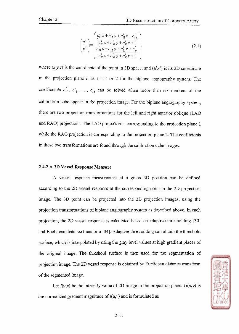
Chapter 2 3D Reconstruction of Coronary Artery
+ c^y + + c14
+ + + ̂ 24 c^x + c^y + c^z-hl
(2.1)
where (xfyfz) is the coordinate of the point in 3D space, and (u l}v l) is its 2D coordinate
in the projection plane / , a s / = 1 or 2 for the biplane angiography system. The
coefficients c“,c|2,…,c; can be solved when more than six markers of the
calibration cube appear in the projection image. For the biplane angiography system,
there are two projection transformations for the left and right anterior oblique (LAO
and RAO) projections. The LAO projection is corresponding to the projection plane 1
while the RAO projection is corresponding to the projection plane 2. The coefficients
in these two transformations are found through the calibration cube images.
2.4.2 A 3D Vessel Response Measure
A vessel response measurement at a given 3D position can be defined
according to the 2D vessel response at the corresponding point in the 2D projection
image. The 3D point can be projected into the 2D projection images, using the
projection transformations of biplane angiography system as described above. In each
projection, the 2D vessel response is calculated based on adaptive thresholding [30]
and Euclidean distance transform [34]. Adaptive thresholding can obtain the threshold
surface, which is interpolated by using the gray level values at high gradient places of
the original image. The threshold surface is then used for the segmentation of
projection image. The 2D vessel response is obtained by Euclidean distance transform
of the segmented image.
Let /(w,v) be the intensity value of 2D image in the projection plane. G{u,v) is
the normalized gradient magnitude of /(w,v) and is formulated as
2-11

Chapter 2 3D Reconstruction of Coronary Artery
, |W(i/,v)| V ) - max^V/(H?v)|) • ( 2 . 2 )
The segmented image L(u , v) may be defined as
JO, if I(u,v)<x{u,v) L{u,v) - ^ (2.3)
[1, if I{u,v)>x{u,v)
where x(u,v) is the threshold surface at the point (w,v) in the projection plane. I{u,v)
and T(W,V) are two surfaces which intersect at positions C = { ( I / , V ) | / ( W , V ) = T ( W 5 V ) } . C
should define the locations of the object boundaries. That means if T(U,V) is the right
threshold surface, J G{u,v)dHx{u,v)JC should be a maximum, wherein1 is the 1-D
Hausdorff measure supported by c, and C is the number of object boundary points.
This necessitates in finding t in a function space Q to
minf F(x)dH\u,v)/c, (2.4) xeQ. Jc f
where F(T) = -G(u,v),(u,V)E C.
To solve this problem, a penalty term should be introduced into the object
function for regularisation. Then the object function to be minimised is
)dHl ( w , v ) + 入 J J du
+ 9v
dudv , (2.5)
where X is the regularisation parameter. Minimising (2.5) is equal to solving the
following Poisson equation:
f 8F(t) • “ 、 • 2 咖 , 和 a I , l f ( “ , V ) e c . (2.6)
[0 ,otherwise
Here, a=(\l2)X. Since F{x) relates to c, F(t) can be written as B y the
chain rule,
2-12
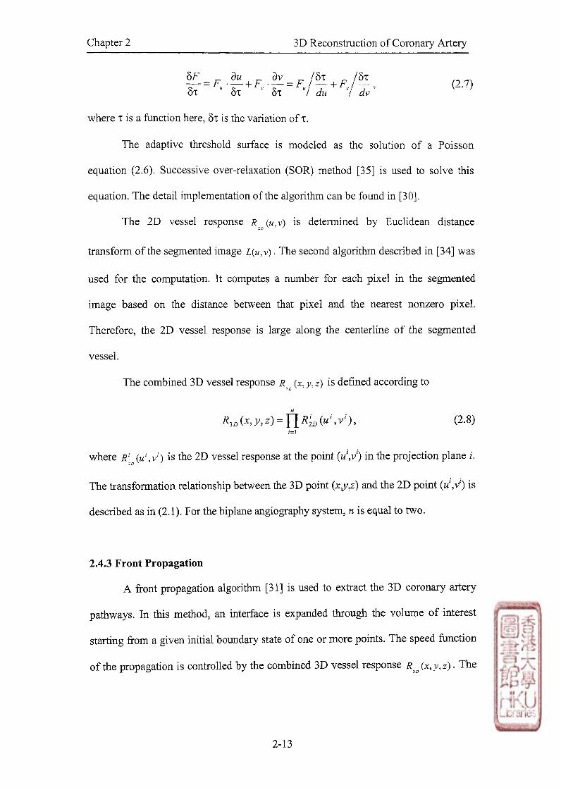
Chapter 2 3D Reconstruction of Coronary Artery
5F du dv /8x /8t - 5 + 〜 ( 2 . 7 )
where T is a function here, 5t is the variation of T.
The adaptive threshold surface is modeled as the solution of a Poisson
equation (2.6). Successive over-relaxation (SOR) method [35] is used to solve this
equation. The detail implementation of the algorithm can be found in [30].
The 2D vessel response R 丨)(u,v) is determined by Euclidean distance
transform of the segmented image L(u,v). The second algorithm described in [34] was
used for the computation. It computes a number for each pixel in the segmented
image based on the distance between that pixel and the nearest nonzero pixel.
Therefore, the 2D vessel response is large along the centerline of the segmented
vessel.
The combined 3D vessel response R 。(X, y,z) is defined according to
R w { x , y , z ) = Y \ R l2 D ( u \ v l ) , (2.8)
/=1
where R[d (w、v' ) is the 2D vessel response at the point {u\vl) in the projection plane /•
The transformation relationship between the 3D point (x,y,z) and the 2D point (u\vl) is
described as in (2.1). For the biplane angiography system,n is equal to two.
2.4.3 Front Propagation
A front propagation algorithm [31] is used to extract the 3D coronary artery
pathways. In this method,an interface is expanded through the volume of interest
starting from a given initial boundary state of one or more points. The speed function
of the propagation is controlled by the combined 3D vessel response (x, y, z) • The
2-13
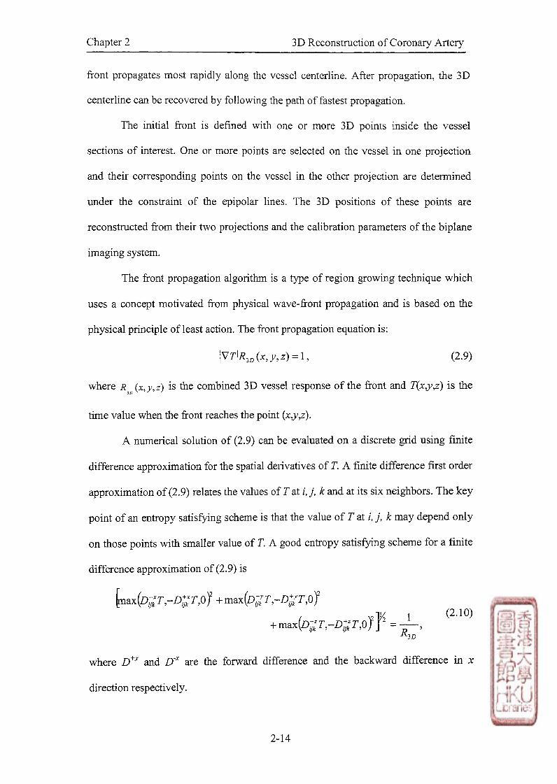
Chapter 2 3D Reconstruction of Coronary Artery
front propagates most rapidly along the vessel centerline. After propagation, the 3D
centerline can be recovered by following the path of fastest propagation.
The initial front is defined with one or more 3D points inside the vessel
sections of interest. One or more points are selected on the vessel in one projection
and their corresponding points on the vessel in the other projection are determined
under the constraint of the epipolar lines. The 3D positions of these points are
reconstructed from their two projections and the calibration parameters of the biplane
imaging system.
The front propagation algorithm is a type of region growing technique which
uses a concept motivated from physical wave-front propagation and is based on the
physical principle of least action. The front propagation equation is:
\VT\Rw{x,y,z) = l , (2.9)
where R^{x,y,z) is the combined 3D vessel response of the front and T{x,y )̂ is the
time value when the front reaches the point
A numerical solution of (2.9) can be evaluated on a discrete grid using finite
difference approximation for the spatial derivatives of T. A finite difference first order
approximation of (2.9) relates the values of T at i, j , k and at its six neighbors. The key
point of an entropy satisfying scheme is that the value of T at i, j, k may depend only
on those points with smaller value of L A good entropy satisfying scheme for a finite
difference approximation of (2.9) is
+ m a x ( D ^ r ^ r ? o ) 2
( i (2.10) + m a x ( A ^ r ? ^ r ? o ; f 2 = — ?
火3D
where Z)+x and n x are the forward difference and the backward difference in x
direction respectively.
2-14
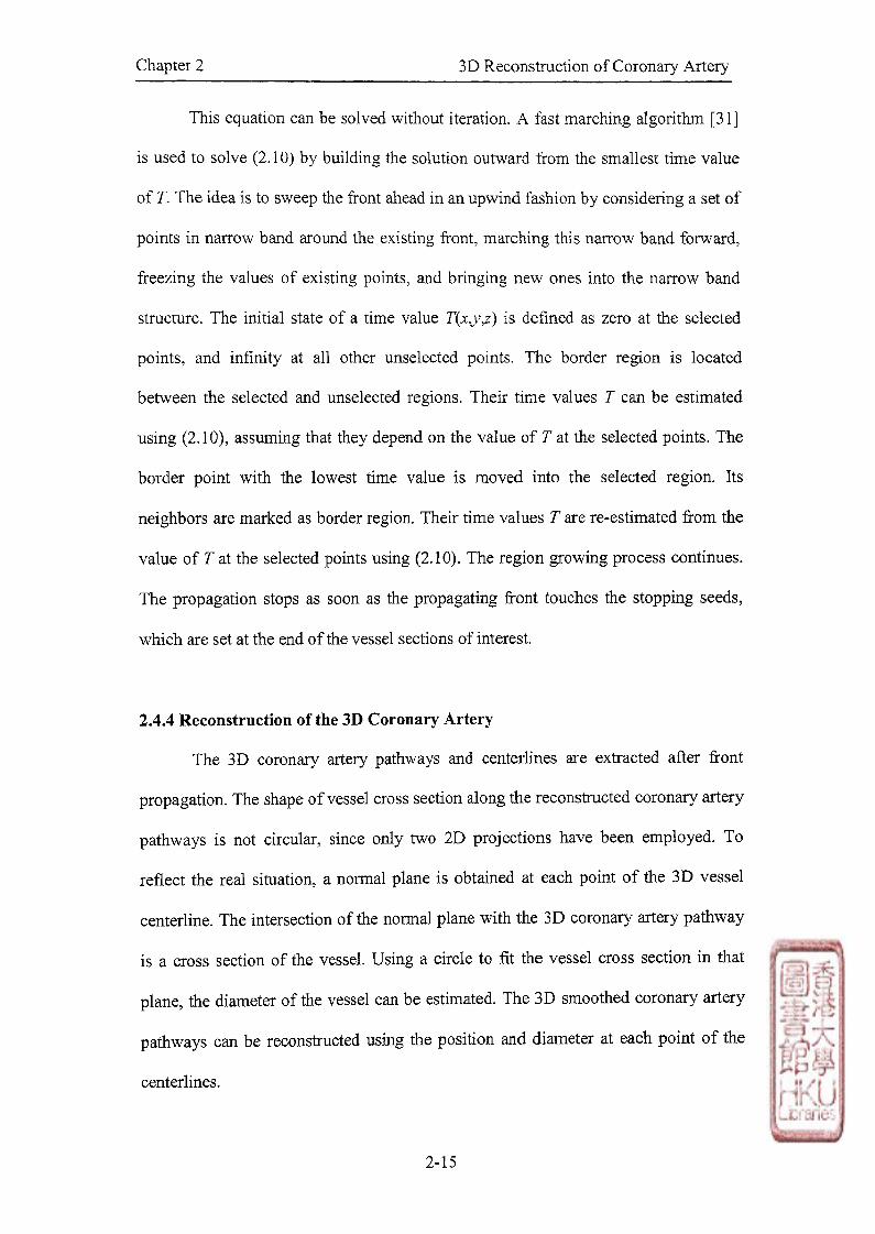
Chapter 2 3D Reconstruction of Coronary Artery
This equation can be solved without iteration. A fast marching algorithm [31]
is used to solve (2.10) by building the solution outward from the smallest time value
of T. The idea is to sweep the front ahead in an upwind fashion by considering a set of
points in narrow band around the existing front, marching this narrow band forward,
freezing the values of existing points, and bringing new ones into the narrow band
structure. The initial state of a time value T(x,y,z) is defined as zero at the selected
points, and infinity at all other unselected points. The border region is located
between the selected and unselected regions. Their time values T can be estimated
using (2.10),assuming that they depend on the value of T at the selected points. The
border point with the lowest time value is moved into the selected region. Its
neighbors are marked as border region. Their time values T are re-estimated from the
value of T at the selected points using (2.10). The region growing process continues.
The propagation stops as soon as the propagating front touches the stopping seeds,
which are set at the end of the vessel sections of interest.
2.4.4 Reconstruction of the 3D Coronary Artery
The 3D coronary artery pathways and centerlines are extracted after front
propagation. The shape of vessel cross section along the reconstructed coronary artery
pathways is not circular, since only two 2D projections have been employed. To
reflect the real situation, a normal plane is obtained at each point of the 3D vessel
centerline. The intersection of the normal plane with the 3D coronary artery pathway
is a cross section of the vessel. Using a circle to fit the vessel cross section in that
plane, the diameter of the vessel can be estimated. The 3D smoothed coronary artery
pathways can be reconstructed using the position and diameter at each point of the
centerlines.
2-15

Chapter 2 3D Reconstruction of Coronary Artery
The direction of vessel of a point is determined by the coordinates of that point
and its neighboring point along the 3D vessel centerline. The normal plane is defined
by a plane perpendicular to the vessel direction at each point of the vessel centerline.
Instead of finding a normal plane, the 3D coronary artery pathway can be translated
and rotated [36] to a new position such that a point of the vessel centerline is relocated
to the coordinate origin and its vessel direction is along with i axis. Then the xy plane
becomes the normal plane of the 3D coronary artery pathway at that point of the
vessel centerline.
A point P\ and its neighboring point Pt are extracted along the 3D vessel
centerline. The vessel direction is defined by a vector V pointing from P\ to 尸2 as
( Z 1 1 ) = (x2 -x15J;2-yx ,z1 - A )
A unit vector u is then defined as
V = (2.12)
where the components “1, “2,and <33 of the unit vector u are the direction cosines of
the vector:
x〗一 _ y 2 — c " ) 1 七 = _ | ^ ,
( .
3 )
The first step in the transformation is to set up the translation matrix that
translates the vector so that it passes through the coordinate origin. This can be
accomplished by moving Pi to the coordinate origin. The translation matrix is
1 0 0 — Xj 0 1 0 - 凡
0 0 1 — Zj 0 0 0 1
(2.14)
2-16
Chapter 2 3D Reconstruction of Coronary Artery
The vector can be put on the z axis by two more steps. The vector is
transformed into the xz plane by rotating about the x axis. This is achieved by the
following rotation matrix:
0 0
(2.15)
where + a\ • Then the vector is aligned with the z axis by rotating about the
y axis. This is realized by the following rotation matrix:
0 1 0 0 al 0 a4 0 0 0 0 1
(2.16)
To complete the translation and rotation of the 3D coronary artery pathway,
the transformation matrix can be expressed as the composition of the above three
transformations:
•M, (2.17)
Hence, the 3D coronary artery pathway is transformed to a new position such
that the xy plane becomes the normal plane. The intersection of the xy plane with the
3D coronary artery pathway is a cross section of the vessel at the point of the vessel
centerline. The area of vessel cross section is measured. Assuming that the vessel
cross section is circular, the diameter of the vessel can be estimated by the following
equation:
AA (2.18)
where d and A are the diameter and area of the vessel cross section respectively.
2-17

Chapter 2 3D Reconstruction of Coronary Artery
2.5 Validation
To test the capability and accuracy of the new approach for the 3D
reconstruction of coronary artery in biplane angiography, a coronary arterial phantom
[2] was used for validation. A coronary arterial phantom mimicking the 3D course of
an idealized left anterior descending coronary artery portion was made. It is 3mm
diameter radio-opaque wire solder embedded on the side surface of a Plexiglas
cylinder as shown in Fig. 2.2. The cylinder is 35mm in height and 88mm in diameter,
comparable to the dimensions of a human heart.
Fig. 2.2 A coronary arterial phantom. The thick dark curve is a radio-opaque wire
solder mimicking the 3D course of an idealized left anterior descending
coronary artery portion [2].
The coronary arterial phantom was placed in the angiography system at a
position corresponding to that of a patient's heart during catheterization. Projection
images of the phantom were taken, together with the calibration images. The new
approach was applied to reconstruct the 3D vessel phantom.
2-18

Chapter 2 3D Reconstruction of Coronary Artery
2.6 Results
In this section, performance of the proposed approach is shown. Our study is
based on biplane cineangiograms acquired during clinical catheterization at the Duke
University Medical Center, using Philips Polydiagnostic C-arm biplane angiography
systems. It consists of three parts. The first part is to compare the fixed thresholding
method and adaptive thresholding method in the segmentation of coronary artery in
the projection images. The second part gives the validation results of the coronary
arterial phantom. It shows the capability and accuracy of the new approach for the 3D
reconstruction of coronary artery in biplane angiography. The third part shows the
experimental results of the new 3D reconstruction approach applied to the biplane
angiograms of human coronary arteries.
2.6.1 Comparisons of Fixed Thresholding and Adaptive Thresholding
The fixed thresholding method [29] and adaptive thresholding method [30]
were compared in the segmentation of coronary artery in the projection images. There
are left and right anterior oblique (LAO and RAO) projection pairs in the biplane
angiograms of coronary artery. In Fig. 2.3, the fixed thresholding method and
adaptive thresholding method were applied to the segmentation of coronary artery in
the LAO projection image. The black region is the segmented vessel while the white
region is the background. Similarly, both methods were applied to the segmentation of
coronary artery in the RAO projection image as shown in Fig. 2 A
2-19
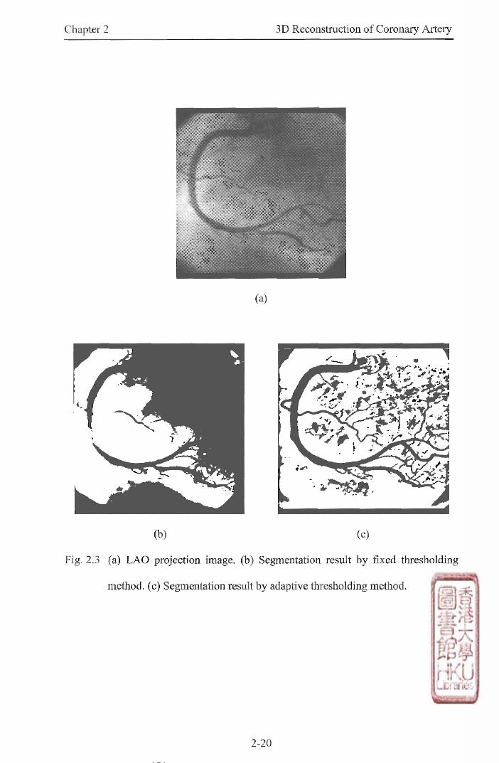
Chapter 2 3D Reconstruction of Coronary Artery
(b) (c)
Fig. 2.3 (a) L A O projection image, (b) Segmentation result by fixed thresholding
method, (c) Segmentation result by adaptive thresholding method.

Chapter 2 3D Reconstruction of Coronary Artery
(a)
(b) (c)
Fig. 2.4 (a) RAO projection image, (b) Segmentation result by fixed thresholding
method, (c) Segmentation result by adaptive thresholding method.
2-21
Chapter 2 3D Reconstruction of Coronary Artery
2.6.2 Results of Validation with the Coronary Arterial Phantom
A 3D coronary arterial phantom was reconstructed from two 2D projection
images. Fig. 2.5 shows the left and right anterior oblique (LAO and RAO) projection
pairs of a coronary arterial phantom (Phantom 1). The vessel phantom has lower gray
level values than its surroundings. The phantom can be easily segmented by most
thresholding methods such as fixed thresholding or adaptive thresholding. As seen
from Fig. 2.6,the vessel phantoms were well segmented in both projection images.
The 2D vessel response was obtained by Euclidean distance transform of the
segmented images. The 3D coronary arterial phantom and its centerline were
extracted using front propagation controlled by the combined 3D vessel response. Fig.
2.7 shows the 3D reconstructed centerline of coronary arterial phantom projected back
to the LAO and RAO projection images. The 3D smoothed coronary arterial phantom
was reconstructed using the position and diameter at each point of the centerline. The
mean and standard deviation of the calculated diameter were 2.930mm and 0.205mm
respectively. The percentage error was 2.33% when compared with the actual
diameter of coronary arterial phantom.
2-22

Chapter 2 3D Reconstruction of Coronary Artery
⑻ (b)
Fig. 2.5 (a) LAO and (b) RAO projection pairs of a coronary arterial phantom.
(a) (b)
Fig. 2.6 Segmentation results of the (a) LAO and (b) RAO projection images.
2-23

Chapter 2 3D Reconstruction of Coronary Artery
(a) (b)
Fig. 2,7 The 3D reconstructed centerline of coronary arterial phantom projected back
to the (a) L A O and (b) RAO projection images.
Similarly, the proposed approach was applied to the projection images of the
same phantom taken at a different acquisition angle. Fig. 2.8 shows the left and right
anterior oblique (LAO and RAO) projection pairs of a coronary arterial phantom
(Phantom 2). Fig. 2.9 shows the segmentation results of vessel phantoms in both
projection images. Fig. 2.10 shows the 3D reconstructed centerline of coronary
arterial phantom projected back to the LAO and RAO projection images. The mean
and standard deviation of the calculated diameter were 2.863mm and 0.247mm
respectively. The percentage error was 4.57% when compared with the actual
diameter of coronary arterial phantom. Table 2.1 summarizes the results of validation
with the coronary arterial phantom.
2-24
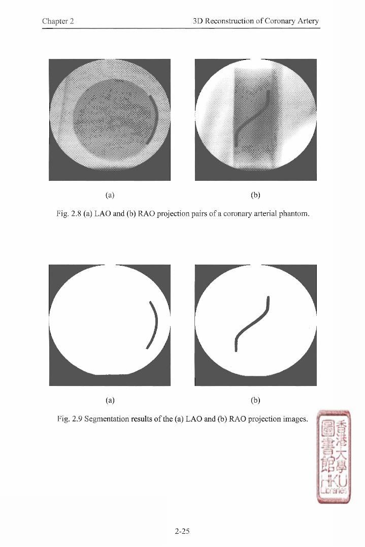
Chapter 2 3D Reconstruction of Coronary Artery
(a) (b)
Fig. 2.8 (a) L A O and (b) RAO projection pairs of a coronary arterial phantom.
(a) (b)
Fig. 2.9 Segmentation results of the (a) LAO and (b) RAO projection images.
2-25

Chapter 2 3D Reconstruction of Coronary Artery
(a) (b)
Fig. 2.10 The 3D reconstructed centerline of coronary arterial phantom projected back
to the (a) LAO and (b) RAO projection images.
Diameter
Phantom
Actual value
(mm)
Mean of
calculated value
(mm)
Standard deviation
of calculated value
(mm)
Percentage
error
Phantom 1 3.000 2.930 0.205 2.33%
Phantom 2 3.000 2.863 0.247 4,57%
Table 2.1 Results of validation with the coronary arterial phantom.
2.6.3 Results of Coronary Artery Reconstruction
A 3D coronary artery pathway was reconstructed from two 2D projection
images. Fig. 2.11 shows the left and right anterior oblique (LAO and RAO) projection
pairs of a right coronary artery (RCA). The segmentation results of adaptive
thresholding applied to the LAO and RAO projection images were given in Fig. 2.12.
2-26
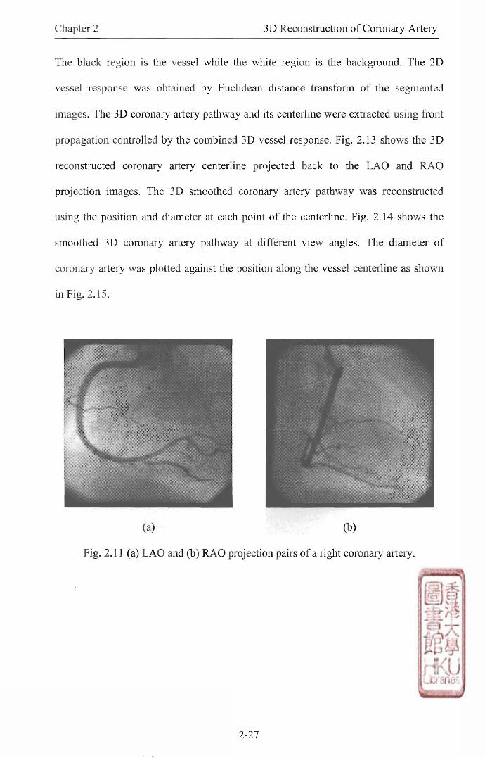
Chapter 2 3D Reconstruction of Coronary Artery
The black region is the vessel while the white region is the background. The 2D
vessel response was obtained by Euclidean distance transform of the segmented
images. The 3D coronary artery pathway and its centerline were extracted using front
propagation controlled by the combined 3D vessel response. Fig. 2.13 shows the 3D
reconstructed coronary artery centerline projected back to the LAO and RAO
projection images. The 3D smoothed coronary artery pathway was reconstructed
using the position and diameter at each point of the centerline. Fig. 2.14 shows the
smoothed 3D coronary artery pathway at different view angles. The diameter of
coronary artery was plotted against the position along the vessel centerline as shown
in Fig. 2.15.
(a) (b)
Fig. 2.11 (a) LAO and (b) RAO projection pairs of a right coronary artery
2-27
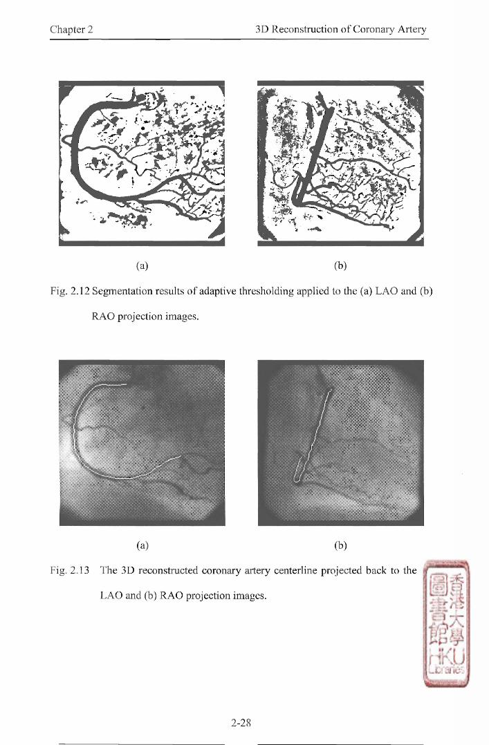
Chapter 2 3D Reconstruction of Coronary Artery
r •
(a) (b)
Fig. 2.12 Segmentation results of adaptive thresholding applied to the (a) LAO and (b)
RAO projection images.
(a) (b)
Fig. 2.13 The 3D reconstructed coronary artery centerline projected back to the (a)
LAO and (b) RAO projection images.
2-28
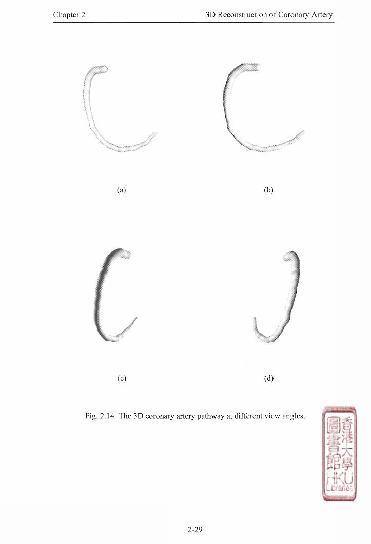
Chapter 2 3D Reconstruction of Coronary Artery
⑻ (b)
(c) (d)
Fig. 2.14 The 3D coronary artery pathway at different view angles.
2-29

Chapter 2 3D Reconstruction of Coronary Artery
0 20 40 60 80 100 120 Position along vessel centerline《mm)
Fig. 2.15 The diameter of coronary artery plotted against the position along vessel
centerline.
The proposed approach was then applied to another case of left coronary
artery (LCA). Fig. 2.16 shows the left and right anterior oblique (LAO and RAO)
projection pairs of a left coronary artery. Since this patient has a big body, the contrast
of the lateral projected image (RAO image) is significantly degraded when compared
with the LAO image. However, our adaptive thresholding algorithm still worked well
for both images as shown in Fig. 2.17. Similarly,the smoothed 3D coronary artery
pathway and its centerline were reconstructed. Fig. 2.18 shows the 3D reconstructed
coronary artery centerline projected back to the LAO and RAO projection images. Fig.
2.19 shows the smoothed 3D coronary artery pathway at different view angles. The
diameter of coronary artery was plotted against the position along the vessel
centerline as shown in Fig. 2.20.
(UIE)
tBJg AJeuoJO
O
lo JBaEeQ
2-30
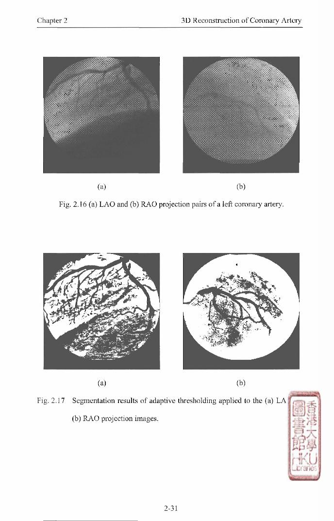
Chapter 2 3D Reconstruction of Coronary Artery
(a) (b)
Fig. 2.】6 (a) LAO and (b) RAO projection pairs of a left coronary artery.
(a) (b)
Fig. 2.17 Segmentation results of adaptive thresholding applied to the (a) LAO and
(b) RAO projection images.
2-31
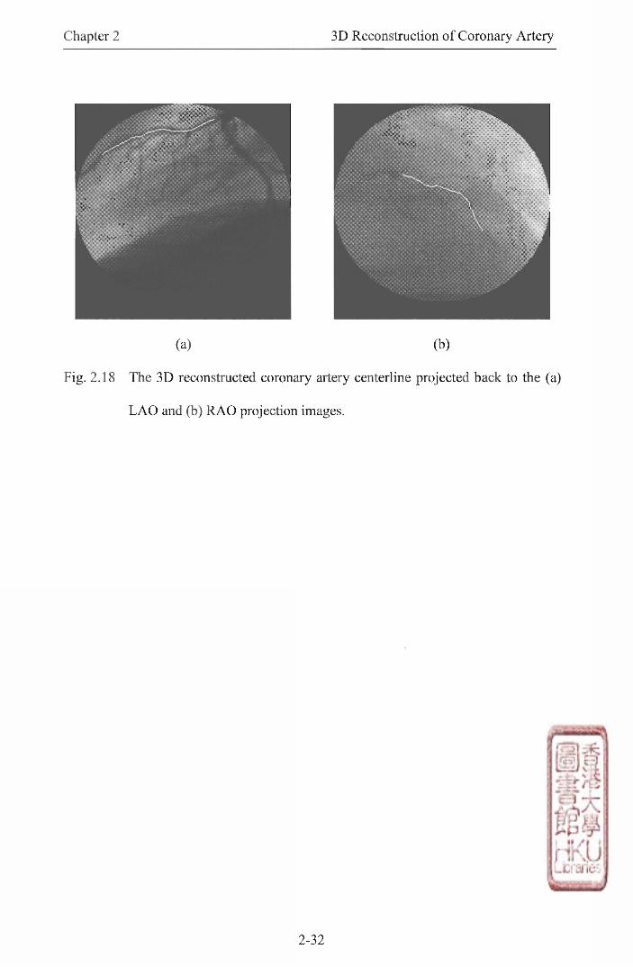
Chapter 2 3D Reconstruction of Coronary Artery
(a) (b)
Fig. 2.18 The 3D reconstructed coronary artery centerline projected back to the (a)
L A O and (b) RAO projection images.
2-32
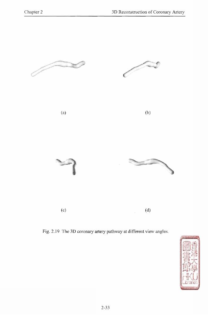
Chapter 2 3D Reconstruction of Coronary Artery
(a) (b)
(c) (d)
Fig. 2.19 The 3D coronary artery pathway at different view angles.
2-33
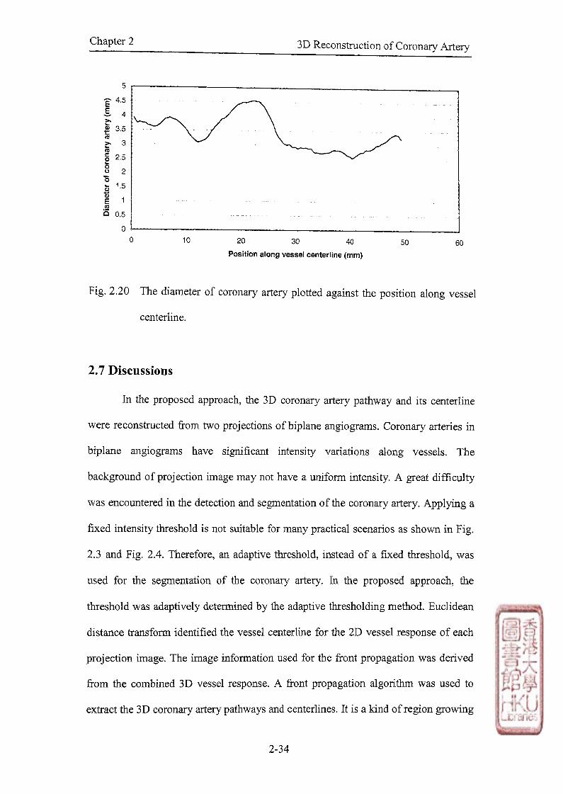
o 10 20 30 40 50 60
Position along vessel centerline (mm)
Fig. 2.20 The diameter of coronary artery plotted against the position along vessel
centerline.
2.7 Discussions
In the proposed approach, the 3D coronary artery pathway and its centerline
were reconstructed from two projections of biplane angiograms. Coronary arteries in
biplane angiograms have significant intensity variations along vessels. The
background of projection image may not have a uniform intensity. A great difficulty
was encountered in the detection and segmentation of the coronary artery. Applying a
fixed intensity threshold is not suitable for many practical scenarios as shown in Fig.
2.3 and Fig. 2.4. Therefore, an adaptive threshold, instead of a fixed threshold,was
used for the segmentation of the coronary artery. In the proposed approach, the
threshold was adaptively determined by the adaptive thresholding method. Euclidean
distance transform identified the vessel centerline for the 2D vessel response of each
projection image. The image information used for the front propagation was derived
from the combined 3D vessel response. A front propagation algorithm was used to
extract the 3D coronary artery pathways and centerlines. It is a kind of region growing
Chapter 2 — 3D Reconstruction of Coronary Artery
2-34
Chapter 2 3D Reconstruction of Coronary Artery
technique which uses a concept motivated from physical wave-front propagation and
is based on the physical principle of least action. This front propagation algorithm was
originally developed to work on 2D space and it was extended to operate on 3D space
for the vessel reconstruction in this case. Actually, it is possible to farther extend it to
work on 4D space. Then the temporal information of the 3D coronary artery pathways
and centerlines could be incorporated for the tracking of 3D coronary artery motion in
the future research and development.
There is an advantage of the proposed approach over those methods which
reconstruct the vessel pathways from 2D or 3D centerlines [3], [25]-[27] based on the
2D vessel analysis. In the proposed approach, the 3D coronary artery pathways and
centerlines are extracted after front propagation. Then the vessel diameter is estimated
along the extracted 3D centerlines based on the reconstructed 3D coronary artery
pathways. Therefore, the 3D smoothed coronary artery pathways are reconstructed
based on the 3D vessel analysis rather than the 2D vessel analysis. The problems of
vessel overlap and foreshortening in the 2D vessel analysis wil l be minimized.
The capability of the proposed approach for the 3D reconstruction of coronary
artery in biplane angiography was validated using a coronary arterial phantom
mimicking a coronary artery. The validations have shown that the proposed approach
can reliably reconstruct the 3D coronary artery pathways and centerlines from two 2D
projection images,and accurately quantify the diameter of the vessel In the results of
the 3D coronary artery reconstruction, the smoothed 3D coronary artery pathways and
centerlines were well reconstructed from two 2D projection images. The diameter of
the vessel was also estimated along the 3D vessel centerline. The estimated vessel
diameter will provide vital information for the research and treatment of coronary
artery disease.
2-35

Chapter 2 3D Reconstruction of Coronary Artery
The image information from two 2D projection images is combined for the
reconstruction of 3D coronary artery pathways. Effects of vessel overlap and
foreshortening in individual projections are mostly minimized by combining
information from the two projection images. Further improvement on the
reconstruction results will be obtained i f better quality projections, with less vessel
overlap, can be used for the reconstruction of the 3D coronary artery pathways. The
traditional trial and error method provides views in which overlapping and
foreshortening are minimized, depending on the subjective experience-based
judgment of the angiographer [5]. The patient, however, might receive substantial
radiation and contrast materials during diagnostic and interventional procedures. The
optimal view strategy [37],[38] has been developed for the minimization of vessel
overlap and foreshortening.
2.8 Summary
In this chapter, a new approach has been presented for the 3D reconstruction
and visualization of coronary arteries in biplane angiography. The front propagation
algorithm was applied to extract the 3D coronary artery pathways and centerlines. The
vessel diameter was determined along vessel centerlines. The 3D smoothed coronary
artery pathways were reconstructed using vessel centerlines and diameter.
Experimental results showed that 3D coronary arteries were successfully
reconstructed from two projections of biplane angiograms. The capability and
accuracy of the proposed approach was validated using a coronary arterial phantom. It
can be further developed for the quantitative analysis of coronary artery in biplane
angiography.
2-36

Chapter 2 3D Reconstruction of Coronary Artery
2.9 References
[1] T. V . Nguyen and J. Sklansky, “Reconstructing the 3-D medical axes of
coronary arteries in single-view cineangiograms;' IEEE Trans. Med. Imag., vol.
13,pp. 61-73, 1994.
[2] Z. Ding, and M. H. Friedman, "Quantification of 3-D Coronary Arterial Motion
Using Clinical Biplane Angiograms," InL J. Cardiac Imag” vol. 16, pp. 331-346,
2000.
[3] S. Young, B. Movassaghi,J. Weese, and V. Rasche, “3D vessel axis extraction
using 2D calibrated x-ray projections for coronary modeling," in Proc. SPIE,
2003.
[4] F. Cheriet,J. Meunier, J. Lesperance, and M. Bertrand, "Self-calibration of a
stereo system using matched points: Application to biplane X-ray imaging," in
Proc. SPIE, vol. 2354,1994,pp. 279-289.
[5] S. J. Chen and J. D. Carroll, “3-D reconstruction of coronary arterial tree to
optimize angiographic visualization," IEEE Trans. Med. Imag” vol. 19,pp. 318-
336,2000.
[6] S. Stansfield,“ANGI: A rule based expert system for automatic segmentation of
coronary vessels from digital subtracted angiograms,,,IEEE Trans. Pattern Anal.
Machine Intell, vol. 8, pp. 188-199, 1986.
[7] C. Smets, F. Vandewerf, P. Suetens, and A. Oosterlixick,"An expert system for
the labeling and 3D reconstruction of the coronary arteries from two
projections," Int. J. Cardiac Imag” vol. 5,pp. 145-154,1990.
[8] M. Garreau, J. L. Coatrieux, R. Collorec, and C. Chardenon, “A knowledge-
based approach for 3D reconstruction and labeling of vascular networks from
2-37
Chapter 2 3D Reconstruction of Coronaiy Artery
biplane angiographic projections,” IEEE Trans. Med. Imag” vol. 10, pp. 122-
131,1991.
[9] G. Coppini, M. Demi, R. Mennini, and G. Valli, “3D knowledge driven
reconstruction of coronary trees," Med. Biol Eng. Comput., vol. 29, pp. 535-542,
1991.
[10] D. Delaere, C. Smets, P. Suetens,G. Marchal, and F. Van de Werf,
"Knowledge-based system for the 3D reconstruction of blood vessels from two
angiographic projections," Med. Biol Eng. Comput ., vol. 29,pp. 27-36,1991.
[11] J. A. Fessler and A. Macovski,“Object-based 3D reconstruction of arterial trees
from magnetic resonance angiograms," IEEE Trans. Med. Imag., vol. 10,pp.
25-39, 1991.
[12] 1. Liu and Y. Sun, “Fully automated reconstruction of 3D vascular tree
structures from two orthogonal views using computational algorithms and
production rules,” Opt. Eng., vol. 31, pp. 2197-2207,1992.
[13] K. Haris, S. N. Efstratiadis, N. Maglaveras,C. Pappas, J. Gourassas, and G.
Louridas, “Model-based morphological segmentation and labeling of coronary
angiograms," IEEE Trans. Med. Imag” vol. 18, pp. 1003-1015,1999.
[14] H. C. Kim,B. G. Min,T. S. Lee, S. J. Lee, C. W. Lee, J. H. Park, and C. Han,
“ 3-D digital subtraction angiography," IEEE Trans. Med. Imag ” vol. 1,pp.
152-158, 1982.
[15] D. L. Parker, D. L. Pope, R. van Bree, and H. W. Marshall, “3-D reconstruction
of moving arterial beds from digital subtraction angiography,” Comput Biomed
Res., vol. 20, pp. 166-185, 1987.
2-38
Chapter 2 3D Reconstruction of Coronary Artery
[16] K . Kitamura, J. M. Tobis, and J. Sklansky, “Estimating the 3-D skeletons and
transverse areas of coronary arteries from biplane angiograms;' IEEE Trans.
Med. Imag., vol. 7,pp. 173-187,1988.
[17] T. Saito, M. Misaki, K. Shirato, and T. Takishima, "Three-dimensional
quantitative coronary angiography," IEEE Trans. Biomed. Eng ., vol. 37,pp.
768-777, 1990.
[18] C. P. Pellot, A. Herment, M. Sigelle,P. Horain,H. Maitre,and P. Peronneau, “A
3-D reconstruction of vascular structures from two x-ray angiograms using an
adapted simulated annealing algorithm," IEEE Trans. Med. Imag” vol. 13, pp.
48-60, 1994.
[19] N. Guggenheim, P. A. Doriot,P. A. Dorsaz, P. Descouts, and W. Rutishauser,
“Spatial reconstruction of coronary arteries from angiographic images," Phys.
Med. Biol, vol. 36,pp. 99-110,1991.
[20] C. Seller, R. L. Kirkeeide,and K. L. Gould, “Basic structure-function relations
of the epicardial coronary tree," Circulation, vol. 85, pp. 1987-2003, 1992.
[21] J. L. Coatrieux, J. Rong, and R. Collorec, “A framework for automatic analysis
of the dynamic behavior of coronary angiograms," Int. J. Cardiac Imag., vol. 8,
pp. 1-10, 1992.
[22] Y. Yanagihara, T. Hashimoto, T. Sugahara, and N. Sugimoto, “A new method
for automatic identification of coronary arteries in standard biplane
angiograms," Int J. Cardiac Imag ., vol. 10, pp. 253-261,1994.
[23] A. C. M. Dumay, J. H. C. Reiber, and J. J. Gerbrands, “Determination of
optimal angiographic viewing angles: Basic principles and evaluation study,,,
IEEE Trans. Med. Imag” vol. 13,pp. 13-24,1994.
2-39

Chapter 2 3D Reconstruction of Coronary Artery
[24] G. P. M. Prause, S. C. DeJong,C. R. McKay, and M. Sonka, “Semi-automated
segmentation and 3d reconstruction of coronary trees: Biplane angiography and
intravascular ultrasound data function," in Proc. SPIE, vol. 2709, 1996,pp. 82-
92.
[25] H. Zhu and M. H. Friedman, “Tracking 3-D coronary artery motion with biplane
angiography," in IEEE Int. Symp. on Biomedical Imaging, Washington, DC,
2002, pp. 605-608.
[26] C. Canero, F. Vilarino, J. Mauri, and P. Redeva, "Predictive (un)distortion
model and 3-D reconstruction by biplane snakes,,,IEEE Trans. Med. Imag ., vol.
21, pp. 1188-1201,2002.
[27] C. Sbert and A. F. Sole, “3D curves reconstruction based on deformable
models,” J. Math. Imaging Vis ., vol. 18, pp. 211-223, 2003.
[28] M. Sonka, V. Hlavac, and R. Boyle, Image Processing, Analysis, and Machine
Vision, 2nd ed. Pacific Grove, California: PWS Publishing, 1999.
[29] N. Otsu, “A threshold selection method from gray-level histogram," IEEE Trans.
Syst Man Cybern., vol. 8,pp. 62-66,1979.
[30] F. H. Y. Chan, F. K. Lam, and H. Zhu, "Adaptive thresholding by variational
method,” IEEE Trans. Image Process., vol. 7,pp. 468-473,1998.
[31] J. A. Sethian, Level Set Methods and Fast Marching Methods: Evolving
Interfaces in Computational Geometry, Fluid Mechanics, Computer Vision and
Materials Science. Cambridge: Cambridge University Press, 1999.
[32] B. B. Avants and J. P. Williams, “An adaptive minimal path generation
technique for vessel tracking in CTA/CE-MRA volume images,” in Proc.
MICCAI2000, 2000,pp. 707-716.
2-40
Chapter 2 3D Reconstruction of Coronary Artery
[33] S. Young, V. Pekar, and J. Weese, “Vessel segmentation for visualization of
MRA with blood pool contrast agent,” in Proc. MICCAI 2001 , 2001,pp. 491-
498.
[34] H. Breu, J. Gil,D. Kirkpatrick, and M. Werman, “Linear Time Euclidean
Distance Transform Algorithms,” IEEE Trans. Pattern Anal Machine Intell,
vol. 17, no. 5,pp. 529-533,1995.
[;35] W. H. Press, S. A . Teukolsky, W. T. Vetterling, and B. P. Flannery, Numerical
Recipes in C: The Art of Scientific Computing, 2nd ed. Cambridge: Cambridge
University Press, 1992.
[36] D. Heam and M. P. Baker, Computer Graphics C Version, 2nd ed. Upper Saddle
River, NJ: Prentice Hall,1997, pp. 407-430.
[37] Y. Sato, T. Araki,M. Hanayama,H. Natio, and S. Tamura, “A viewpoint
determination system for stenosis diagnosis and quantification in coronary
angiographic image acquisition,” IEEE Trans. Med. Imag” vol. 17, pp. 121-137,
1998.
[38] S.-Y. J. Chen and J. D. Carroll, “3-D coronary angiography: Improving
visualization strategy for coronary interventions,” in J. H. C. Reiber and E. E.
van der Wall, Eds,What's New in Cardiovascular Imaging, Amsterdam, The
Netherlands: Kluwer, 1998,pp. 61-77.
2-41

Chapter 3 3D Reconstruction of Brain Tumor
Chapter 3
3D Reconstruction of Brain Tumor
from Multislice MR Images
3.1 Preamble
In this chapter, a new approach for the 3D reconstruction of brain tumor in a
series of 2D M R image slices will be presented. The shape and position of tumor in
one slice could be assumed to be similar to that in its neighboring slices. Using this
correlation between consecutive images, the initial plan applied for each slice is
extracted from the resulting boundary of the previous slice. The tumor boundary is
located by a two-step method, which performs region deformation and then contour
deformation, from a fairly rough initial plan. Therefore, only one coarse manual initial
plan is required for the whole series of M R image slices. The tumor is then
reconstructed in 3D space using the located tumor boundary at each slice of the M R
image series. Performance of the proposed approach is evaluated on M R image sets.
Comparisons with manual tracing show the accuracy and effectiveness of the
proposed approach.
3.2 Introduction
Managing non-surgical therapy of brain tumor involves periodic monitoring of
tumor development in terms of area, volume, and shape. Routine magnetic resonance
3-1
Chapter 3 3D Reconstruction of Brain Tumor
(MR) examination gives only a series of two-dimensional (2D) image slices while
subtle changes in the tumor may not be readily noticeable. Although radiologists can
manually trace the tumor boundary in each of the 2D image slices for a rough
estimation of its volume, it is really a tedious and time-consuming process. Routine
application of this process would not be practical. Moreover, the results may not be
consistent and repeatable owing to substantial intra-observer and inter-observer
variability.
A series of parallel 2D M R images produce a 3D representation of the brain
tumor. Successive 2D M R images have some similarities between each other in terms
of size, shape, axis,and gray intensity of the tumor. The change in various properties
of tumor between one image and the next will be small when the slice thickness is
kept within a certain value. In the analysis of successive 2D MR image slices,the
traditional way was to process one by one separately. The correlation between
consecutive images was not taken into consideration. In this chapter,a new approach
for the 3D reconstruction of brain tumor in a series of 2D MR image slices will be
presented. For each of the slice, the initial condition (initial plan) applied is extracted
from the resulting boundary of the previous slice. Then only one coarse manual initial
condition (initial plan) is needed for the whole series of MR image slices. The
information carried within the series of MR image slices is utilized since we treat the
processing of multislice MR images as a 3D problem rather than different separate 2D
problems.
A range of methods has been developed for the processing of medical image
sequences. Zhu and Yan [1] proposed an approach for the detection of brain tumor
boundaries in a series of MR image slices using Hopfield neural network. Mowing et
al [2] proposed an algorithm for recognizing and tracking deformable organs in X-
3-2
Chapter 3 3D Reconstruction of Brain Tumor
ray image sequences based on active contour model. A geometrical constraint was
used, which explicitly introduces a priori knowledge on the expected shape of the
contour. Kang [3] presented a stable snake algorithm for tracking contours in large
M R image sequences. A shape constraint for active contours was introduced to avoid
undesirable deformation effects. However, some methods are not robust enough while
others are limited by constraints or assumptions.
In the proposed approach, a two-step method using region and contour
deformation was applied for the extraction of brain tumor boundary in a series of 2D
M R image slices. Region and contour deformation were derived from the one
introduced in [4] and further developed in [5] and [6]. In the previous work [5],
deformable region model (region deformation) was successfully used to locate the
boundary of brain tumor. The initial plan can be far away from the actual boundary.
The deformable region model [5] is more tolerant to initial plan than the fast snake
method (contour deformation) [7]. However, it is time consuming for computing and
comparing the gray level distribution of the object and its every boundary points. A
fast deformable region model will be proposed for the extraction of brain tumor
boundary. The number of boundary point processed is greatly reduced using a point
sampling technique. Hence, the proposed model can be used as the initial step in
boundary estimation from a coarse initial plan. Then,the detected boundary can be
further refined by the fast snake method [7].
In section 3.3, related research on 3D reconstruction of brain tumor from
multislice MR images is presented. In section 3.4, a new approach for the 3D
reconstruction of brain tumor in a series of 2D MR image slices will be proposed. The
analysis of results will be given in section 3.5. In section 3.6, some experimental
3-3

Chapter 3 3D Reconstruction of Brain Tumor
results will be shown. Section 3.7 gives some discussions. Section 3.8 is the summary
of this chapter.
3.3 Related Research
The purpose of having M R image is to obtain cross section images of 3D brain
tumor at different levels. There are several ways to utilize these brain tumor cross
section images. In the cross section images, the important parameters of brain tumor
may be measured by medical experts for the diagnosis and treatment of brain tumor.
The tumor details, including the position, area and volume of tumor, are vital in the
planning of gamma knife operation. These data are important in determining focus
position in such operation. The analysis results may have the potential to improve
some aspects of the operation's design and procedure. Moreover, the cross section
images may be investigated by medical researchers for the periodic monitoring of
brain tumor. This is significant for the research and investigation of brain tumor
development. Furthermore, some of the cross section images may be analyzed by
medical image processing techniques. The required brain tumor parameters or data
can be extracted for further investigations in the fields of biology, medicine and
science. The processing results are objective and reliable with minimal amount of
human interactions.
The analysis of brain tumor may be performed in 2D or 3D space using the 2D
cross section images. One of the most important medical image processing techniques
is 3D reconstruction. The reconstruction of 3D brain tumor can provide 3D
anatomical information and parameters of the tumor. They are vital for the research
work on brain tumor. As mentioned in Chapter 1,there are mainly two types of 3D
reconstruction: multiview approach and multislice approach. The reconstruction of 3D
3-4

Chapter 3 3D Reconstruction of Brain Tumor
brain tumor from multislice MR images belongs to the multislice approach. Obviously,
more cross section images will give more information for the 3D reconstruction. It
will also increase the acquisition time and encounter more technical difficulties. In
practical application, the slice thickness is from 3mm to 5mm for MRI brain scanning.
The research works in this chapter is focused on the 3D reconstruction of brain tumor
from multislice MR images with such slice thickness.
Although the brain tumor is a 3D entity, it may also be required to analyze the
tumor in 2D space. This can give significant 2D analysis results for the 3D
reconstruction process. Moreover, the 2D anatomical information and parameters of
brain tumor may be needed in some investigations. Therefore, boundary detection of
brain tumor in the 2D cross section images is also an important medical image
processing technique. In this section, some closely related researches on boundary
detection are surveyed and presented.
3.3.1 Boundary Detection
Computer-based boundary detection is a method to extract brain tumor in
medical images. Previous methods [8]-[10] have been widely used in the detection of
various structures in medical images. However, they involve a lot of human
interventions. When these methods are applied to medical images of patient cases,
they lack robustness and encounter difficulties in interactive tuning. The performance
can be improved using active contour model known as “snake,,[4], which locates the
tumor by minimizing the energy function of its boundary. Traditionally, each MR
image required an initial plan to be traced manually for active contour model when
the series of 2D MR images was processed one by one separately. Using the proposed
approach,the initial plan may not be close enough to the actual boundary for the
3-5

Chapter 3 3D Reconstruction of Brain Tumor
active contour model. This model is not robust enough to extract the tumor boundary
in a series of 2D M R images.
Based on active contour model [4], different types of deformable models [11]-
[13] have been developed using edge, region, and shape information of the image.
Some models [7],[14]-[18] used edge information while others [19]-[22] employed
region information. There are two ways in combining the advantages of both models.
One is to use a two-step method [23], [24]. The other is to merge the two aspects into
a function [25]-[28]. Several models [29]-[31] made use of shape information.
For most models using edge information, the initial plan has to be close
enough to the actual boundary. Although the difference in characteristics of tumor
between one slice and the next is small, the distance between actual boundary and
initial plan is still very large for these models. For those using region information,
some models assumed that the gray level of object must be of normal distribution.
Some required the initial plan to be within the object as only growing operation was
used in the deformation process. In tumor boundary extraction using the proposed
approach, a priori knowledge about the shape of tumor cannot be provided for the
model, as the shape can be different from case to case. The initial plan may be inside
or outside the tumor. The gray level of tumor is not normally distributed in most
practical situations. Therefore, the underlying assumption in these models may be
invalid. The shape of brain tumor is random, so those models using shape information
is not suitable in tumor boundary detection.
As mentioned above,some models require the initial plan to be close to the
actual boundary. Moreover, they have difficulties progressing into boundary
concavities. To overcome these, Xu and Prince [15] proposed an external force,
gradient vector flow (GVF), for the active contour model. It is computed as a
3-6
Chapter 3 3D Reconstruction of Brain Tumor
diffusion of the gradient vectors of a gray level or binary edge map derived from the
image. Lie and Chuang [32] developed a no-search movement scheme for the active
contour model with gradient vector flow as the external force. However, other objects
and noise can also give high gray level gradients in the image. The optimization
functions may have many local optima. The extracted boundary will be greatly
dependent on the location of initial plan. Therefore, such models still require the
initial plan to be close enough to the brain tumor.
In multislice M R images, a two-step method using region and contour
deformation is suitable for the extraction of brain tumor boundary using the proposed
approach. Region deformation [5] was successfully used to locate the boundary of
brain tumor. The initial plan can be far away from the actual boundary. Then, the
detected boundary can be further refined by the contour deformation [7]. This can
increase the accuracy of tumor boundary detection.
3.4 Methodology
The new approach is to reconstruct brain tumor in a series of 2D M R image
slices, which is a sequence of parallel 2D images with known separation between each
other. A s the brain is a connected entity,it could be assumed that the shape and
position of tumor in one slice should be similar to that in its neighboring slices. Based
on this assumption, the detected boundary in the current slice can be used as initial
plan for the next slice. Therefore, only one coarse initial plan is required at a
convenient slice with an obvious tumor for the whole series of MR images, instead of
tracing an initial plan manually for each image. The major steps of the new approach
are shown in Fig. 3.1. First,an initial slice is selected from the MR image set and an
initial plan is set manually for tumor boundary detection. Then region and contour
3-7
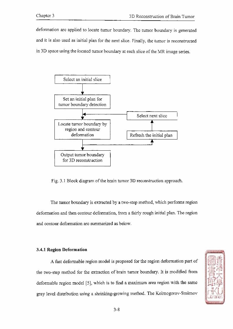
Chapter 3 3D Reconstruction of Brain Tumor
deformation are applied to locate tumor boundary. The tumor boundary is generated
and it is also used as initial plan for the next slice. Finally, the tumor is reconstructed
in 3D space using the located tumor boundary at each slice of the MR image series.
Select next slice
Select an initial slice
Set an initial plan for tumor boundary detection
Output tumor boundary for 3D reconstruction
Locate tumor boundary by region and contour
deformation
Fig. 3.1 Block diagram of the brain tumor 3D reconstruction approach.
The tumor boundary is extracted by a two-step method, which performs region
deformation and then contour deformation, from a fairly rough initial plan. The region
and contour deformation are summarized as below.
3.4.1 Region Deformation
A fast deformable region model is proposed for the region deformation part of
the two-step method for the extraction of brain tumor boundary. It is modified from
deformable region model [5], which is to find a maximum area region with the same
gray level distribution using a shrixiking-growing method. The Kolmogorov-Smimov
3-8

Chapter 3 3D Reconstruction of Brain Tumor
(KS) test method [33] is used to test whether the boundary pixel set and the object
pixel set have the same gray level distribution. The Kolmogorov-Smimov distance D
is defined as
where Fo and FB are the gray level cumulative frequency distribution of object and
boundary respectively. The hypothesis Fo = FB is accepted when D < d, and d is
defined as
where c is the significance level of the test, A is the area of object, and L is the length
of boundary.
When D > d, the region plan covers a region different from the tumor.
Shrinking is performed to deform the region to meet D < d. Hence, the homogeneity
of the region can be guaranteed. The shrinking algorithm is the erosion operation in
mathematical morphology [34]. It only deletes the region boundary elements, which
has a different gray level distribution. In the proposed model, the boundary points are
sampled with intervals of k pixels. Instead of processing all boundary points of the
object, one of every k boundary points will be computed. When D < ?̂ the region plan
covers a region inside the tumor. The region, however, may not cover the whole
tumor. To obtain the maximum area, growing is performed until D 〉 d . The growing
algorithm is the dilation operation of the whole object in mathematical morphology
[34]. The growing algorithm of the proposed model is the same as deformable region
model [5]. After each shrinking and growing, the new region area is compared with
the previous one. If the region area does not change, the process stops; otherwise, the
iteration of shrinking and growing continues.
(3.1)
(3.2)
9
i
3

Chapter 3 3D Reconstruction of Brain Tumor
3.4.2 Contour Deformation
The boundary obtained from region deformation can be further refined by the
fast snake method (contour deformation) [7]. The "snake" method [4] modeled the
contour as an energy-minimizing spline guided by internal and external forces.
i E s m k e = J K (v ⑴ ) + Eext (v ⑷ ) ¼ , (3.3)
o
where v^) = (xO), (̂̂ )) is the parametric equation of the contour, and s is the arc
length.
The internal energy Eint has two parts.
Eint = ( A O ) H O ) | 2 + P O ) | V » | 2 ) / 2 , (3.4)
where and are the first and second order derivatives, respectively. These two
terms are used to control the continuity and smoothness of the contour, with a and (5
representing the weights.
The external energy Eext is from the image edge information. V is the gradient
operator and I is the image. V2/ is the second order derivatives of the image.
^ = Y ( ^ ) l o g ( l + |G a *V 2 / | ) ? (3.5)
where y{s) is the weight and G a is a Gaussian function of the standard deviation a.
The contour v can be represented as a points sequence vo, vi, ..., v/„;, v/, v/+/,...,
vn. vs2 and vss
2 are approximated by v/ [4]. A greedy algorithm has been proposed to
find the minimum energy contour [7]. This algorithm searches for the position of the
minimum energy contour by adjusting each point on the contour during iteration to a
lower energy position in its eight neighbors. The results are comparable with the
variational calculus method [4] and the dynamic programming method [14]. But this
method requires less computation time.
3-10

Chapter 3 3D Reconstruction of Brain Tumor
3.5 Analysis of Results
Results from the proposed approach were compared with those from manual
tracing by the radiologist (P.P. Iu). Double blind method was used in this analysis.
One did not know the results from the other when they performed their own parts. The
result comparison was done afterwards for checking against each other. The
percentage overlapped in area was determined for the results obtained from the
proposed approach and manual tracing in each image. For the manual tracing, the
Paint application from Windows Accessories was used. The image was enlarged to
200% and the radiologist used mouse to draw the tumor boundary with pencil tools in
white color.
3.6 Results
In this section,performance of the proposed approach is shown. It can be
divided into four parts. The first part is to compare the proposed fast deformable
region model and deformable region model with respect to the processing speed in
finding brain tumor boundary in a MR image. The tolerance of the two-step method
will be shown in the second part. The third part is to compare the GVF snake and two-
step method in the extraction of brain tumor boundary in MR image. In the fourth
part, the processing results of different MR image sets using the proposed approach
will be given.
3.6.1 Comparisons of Proposed Model and Deformable Region Model
The proposed fast deformable region model and deformable region model [5]
were implemented using MATLAB code. In the experiments, the significance level of
3-11

Chapter 3 3D Reconstruction of Brain Tumor
the test c was fixed at 3. In the proposed model, the boundary points were sampled
with intervals of k pixels. The values of k tried were ranging from 1 to 15. For k
equals to 1, the proposed model went back to the deformable region model.
Performance of both models was tested using Pentium III PC computer.
A M R image (8-bit grayscale, 256 x 256 pixels) with a brain tumor was used.
The pixel size is 0.898mni x 0.898mm. Circular initial plans were tried, as the shape
of tumor in this image was similar to a circle. In Fig. 3.2a, a circular initial plan
centered at (128,107),with radius 20 pixels, was set outside the brain tumor manually.
The boundary of brain tumor was located using the proposed model with various
settings of h For k equals to 1, the result obtained was that of deformable region
model. While k is small, the resulting boundaries of proposed model were similar to
that of deformable region model. The result difference became larger when k was
larger. Fig. 3.2b shows the resulting boundary when k = 15. The computation time
required by the proposed model was reduced when compared with the deformable
region model. When the computation time required b y the proposed model was
19.4s, nearly one fifth of the time needed by the deformable region model.
In Fig. 3.3a,a circular initial plan centered at (128,107), with radius 10 pixels,
was set inside the brain tumor manually. The boundary of brain tumor was located
using the proposed model with various settings of k. Again, while k is small,both
results were similar. When k became larger, the result difference was larger. Fig. 3.3b
shows the resulting boundary when k = 15. When k = 5,the computation time
required by the proposed model was 13.9s. It was reduced when compared with the
deformable region model. Table 3.1 summaries the computation time required for
different values of k in the brain tumor boundary extraction using two kinds of initial
plans.
3 4 2

Chapter 3 3D Reconstruction of Brain Tumor
⑻ (b)
Fig. 3.2 (a) Initial plan outside the brain tumor, (b) Tumor boundary result from
initial plan shown in (a) for A: = 15.
(a) (b)
Fig. 3.3 (a) Initial plan inside the brain tumor, (b) Tumor boundary result from initial
plan shown in (a) for A: = 15.
3-13

Chapter 3 3D Reconstruction of Brain Tumor
Time Required (s)
k (pixel)
Initial plan outside the
brain tumor
Initial plan inside the
brain tumor
1 88.7 21.9
3 29.6 14.9
5 19.4 13.9
7 17.9 10.6
9 9.8 6.8
11 7.1 3.8
13 6.1 3.6
15 5.9 3.6
Table 3.1 The computation time required for different values of k in the brain tumor
boundary extraction using two kinds of initial plans.
3.6.2 Tolerance of the Two-step Method
The tolerance of the two-step method was tested using a M R image (8-bit
grayscale, 256 x 256 pixels). The pixel size is 0.898min x 0.898xmn. A brain tumor is
contained in the middle of image. The initial plan of tumor boundary was traced
manually as in Fig. 3.4a. The resulting boundary (Fig. 3.4b) was obtained by the two-
step method and fast snake method [7]. The tolerance with respect to the initial plan
was tested in this image. Circular initial plans were tried, as the shape of tumor in this
image was similar to a circle. With the circular initial plan centered at (128,107), the
radius could vary from 9 to 45 pixels (Fig. 3.4c) to generate the result as in Fig. 3.4b
3«14

Chapter 3 3D Reconstruction of Brain Tumor
when using the two-step method. It could only vary from 13 to 16 pixels (Fig. 3.4d)
when using the fast snake method [7].
(c) (d)
Fig. 3.4 (a) Initial plan of tumor boundary, (b) Tumor boundary result from initial
plan shown in (a), (c) Tolerable radius range of circular initial plans of the
two-step method, (d) Tolerable radius range of circular initial plans of the
fast snake method.
3-15

Chapter 3 3D Reconstruction of Brain Tumor
3.6.3 Comparisons of G V F Snake and Two-step Method
The GVF snake [15] and two-step method were compared in the extraction of
brain tumor boundary in M R image. It was tested using a M R image (8-bit grayscale,
256 x 256 pixels). The pixel size is 0.898mm x 0.898mm. A brain tumor is contained
in the middle of image. The initial plan was traced manually outside the brain tumor
as in Fig. 3.5a. The resulting boundary was obtained by GVF snake and two-step
method as shown in Fig. 3.5b and Fig. 3.5c respectively. Similarly,both methods
were applied to extract the brain tumor boundary from an initial plan inside the tumor.
Fig. 3.6 shows the resulting boundaries from both methods.
3 -16
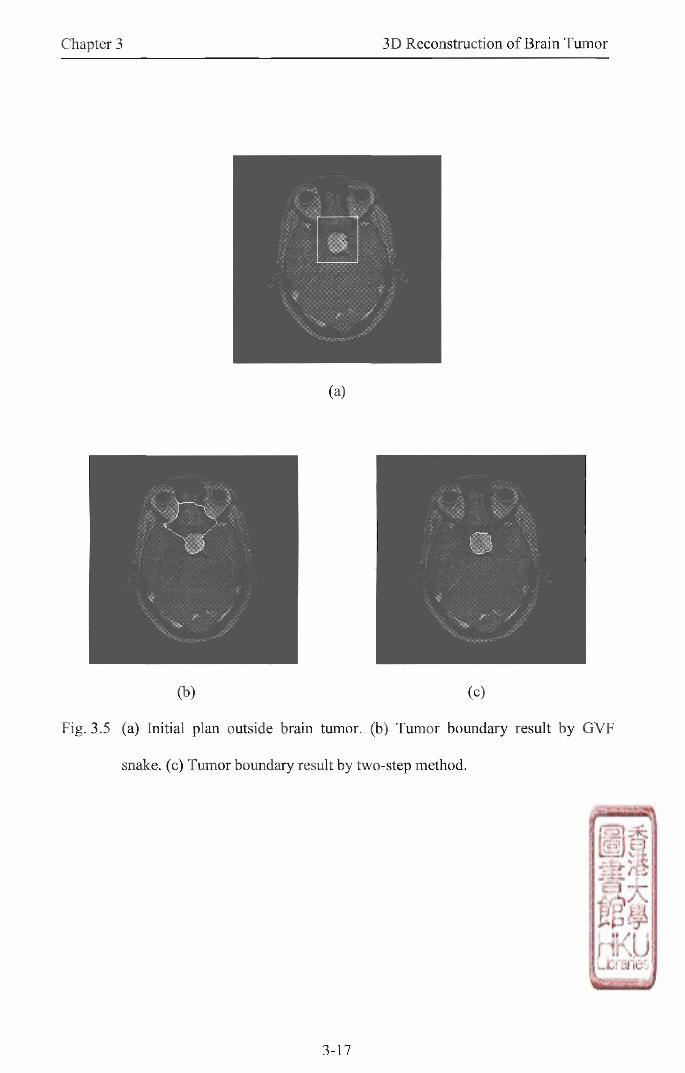
(b) (c)
Fig. 3.5 (a) Initial plan outside brain tumor, (b) Tumor boundary result by GVF
snake, (c) Tumor boundary result by two-step method.
3-17

Chapter 3 3D Reconstruction of Brain Tumor
(a)
(b) (c)
Fig. 3.6 (a) Initial plan inside brain tumor, (b) Tumor boundary result by GVF snake,
(c) Tumor boundary result by two-step method.
3.6.4 Processing of MR Image Sets
In the first experiment, the proposed approach using the two-step method was
applied on a M R image set with 74 slices. Fig. 3.7 shows several selected images
from this set (8-bit grayscale, 256 x 256 pixels). The pixel size of each slice is
3-18
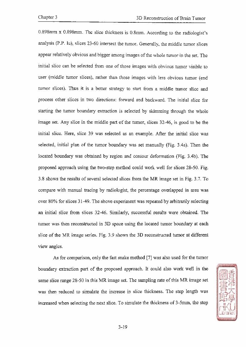
Chapter 3 3D Reconstruction of Brain Tumor
0.898mm x 0.898mm. The slice thickness is 0.8mm. According to the radiologist's
analysis (P.P• Iu), slices 23-60 intersect the tumor. Generally, the middle tumor slices
appear relatively obvious and bigger among images of the whole tumor in the set. The
initial slice can be selected from one of those images with obvious tumor visible to
user (middle tumor slices),rather than those images with less obvious tumor (end
tumor slices). Thus it is a better strategy to start from a middle tumor slice and
process other slices in two directions: forward and backward. The initial slice for
starting the tumor boundary extraction is selected by skimming through the whole
image set. Any slice in the middle part of the tumor, slices 32-46,is good to be the
initial slice. Here, slice 39 was selected as an example. After the initial slice was
selected, initial plan of the tumor boundary was set manually (Fig. 3.4a). Then the
located boundary was obtained by region and contour deformation (Fig. 3.4b). The
proposed approach using the two-step method could work well for slices 28-50. Fig.
3.8 shows the results of several selected slices from the MR image set in Fig. 3.7. To
compare with manual tracing by radiologist, the percentage overlapped in area was
over 80% for slices 31-49. The above experiment was repeated by arbitrarily selecting
an initial slice from slices 32-46. Similarly, successful results were obtained. The
tumor was then reconstructed in 3D space using the located tumor boundary at each
slice of the MR image series. Fig. 3.9 shows the 3D reconstructed tumor at different
view angles.
As for comparison, only the fast snake method [7] was also used for the tumor
boundary extraction part of the proposed approach. It could also work well in the
same slice range 28-50 in this MR image set. The sampling rate of this MR image set
was then reduced to simulate the increase in slice thickness. The step length was
increased when selecting the next slice. To simulate the thickness of 3-5inm,the step

Chapter 3 3D Reconstruction of Brain Tumor
length should be 4-6 slices, corresponding to 3.2-4.8mm. The proposed approach
using the two-step method could work well at any step length from 1 to 6 slices.
When it increased to 4 slices, only using the fast snake method [7] failed.
3-20
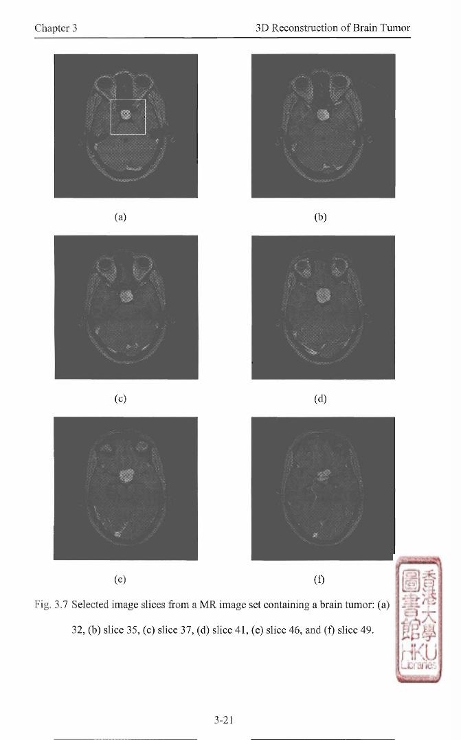
Chapter 3 3D Reconstruction of Brain Tumor
(e) (f)
Fig. 3.7 Selected image slices from a M R image set containing a brain tumor: (a) slice
32,(b) slice 35,(c) slice 37,(d) slice 41,(e) slice 46,and (f) slice 49.
3-21

Chapter 3 3D Reconstruction of Brain Tumor
(e) (f)
Fig. 3.8 Extracted tumor boundaries, superimposed on the original image slices from
the M R image set in Fig. 3.7. Only a portion of the image [the rectangular
region shown in Fig. 3.7a] containing the tumor is shown here: (a) slice 32,
(b) slice 35, (c) slice 37, (d) slice 41,(e) slice 46,and (f) slice 49.
3-22
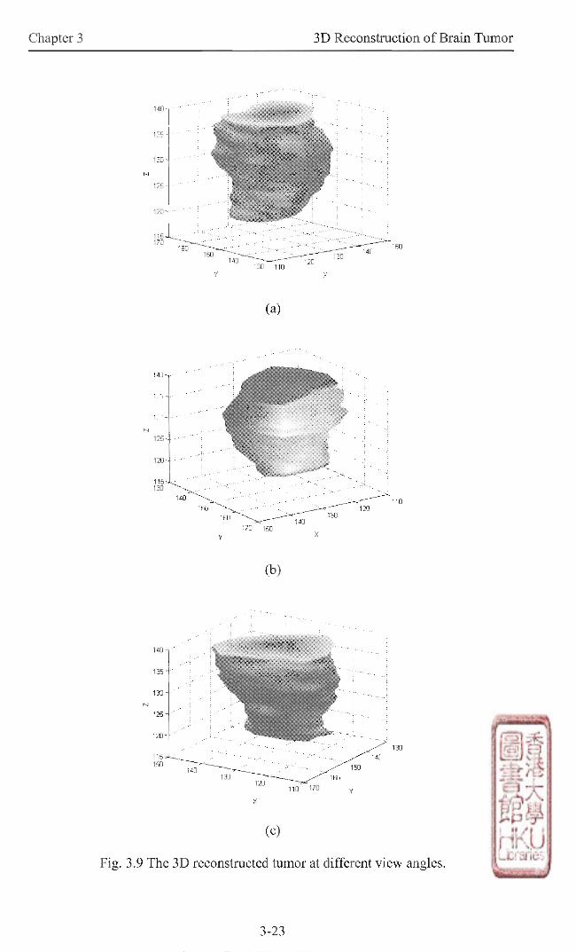
Chapter 3 3D Reconstruction of Brain Tumor
3-23

Chapter 3 3D Reconstruction of Brain Tumor
The second example is a MR image set with 15 slices. Fig. 3.10 shows several
images from this set (8-bit grayscale, 256 x 256 pixels). The pixel size of each slice is
0.977mm x 0.977mm. The slice thickness is 3mm. According to the radiologist's
analysis (P.P. Iu), slices 04-10 intersect the tumor. Slice 07 was chosen as the initial
slice. The proposed approach using the two-step method was used for processing this
M R image set. Fig. 3.11 shows the results of several selected slices from the M R
image set in Fig. 3.10. When compared with manual tracing, the percentage
overlapped in area was over 80% for slices 06-09. The tumor was then reconstructed
in 3D space using the located tumor boundary at each slice of the M R image series.
Fig. 3.12 shows the 3D reconstructed tumor at different view angles.
In the above experiment, the parameters a(s), ^(s), and y(s) in equation (3.4)
and (3.5) were fixed at 1,1,and 10 respectively. Apart from that, there were two more
parameters. One was the parameter c in equation (3.2) for controlling the significance
level in the Kolmogorov-Smimov (KS) test method of region deformation. The other
one was the parameter a in equation (3.5) for controlling the standard deviation of
Gaussian function in the external energy of contour deformation. The values that we
used were chosen by trial and error to give the best estimations of the tumor
boundaries. For the two parameters, c and a , the values tried were ranging from 0.7 to
2.5, and from 2.5 to 4.3 respectively.
3-24

Chapter 3 3D Reconstruction of Brain Tumor
(c) (d)
(Continuing ...)
3-25

Chapter 3 3D Reconstruction of Brain Tumor
(e) (f)
(g)
Fig. 3.10 Selected image slices from another M R image set containing a brain tumor:
(a) slice 04,(b) slice 05,(c) slice 06,(d) slice 07,(e) slice 08,(f) slice 09,
and (g) slice 10.
3-26

Chapter 3 3D Reconstruction of Brain Tumor
3-27
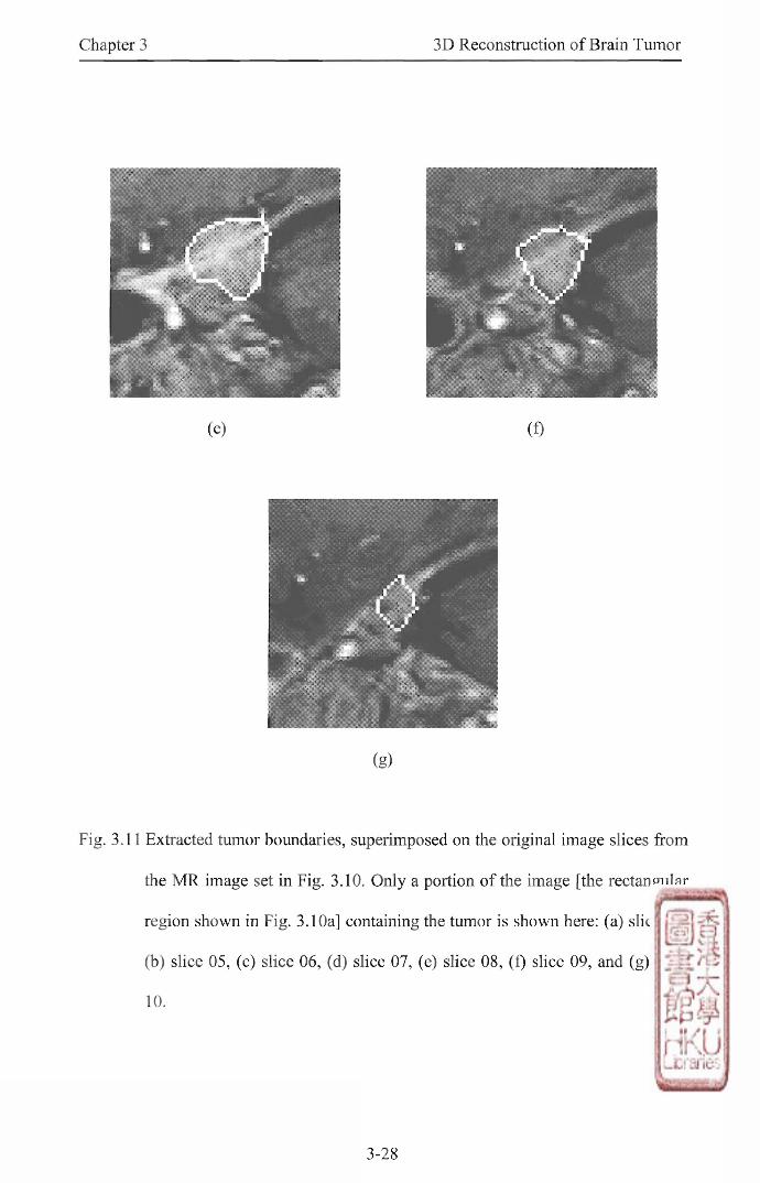
Chapter 3 3D Reconstruction of Brain Tumor
(g)
Fig. 3.11 Extracted tumor boundaries, superimposed on the original image slices from
the M R image set in Fig. 3.10. Only a portion of the image [the rectangular
region shown in Fig. 3.10a] containing the tumor is shown here: (a) slice 04,
(b) slice 05,(c) slice 06,(d) slice 07, (e) slice 08,(f) slice 09, and (g) slice
10.
3-28

Chapter 3 3D Reconstruction of Brain Tumor
(c)
Fig. 3.12 The 3D reconstructed tumor at different view angles.
3-29
Chapter 3 3D Reconstruction of Brain Tumor
3.7 Discussions
The processing speed of the proposed fast deformable region model was tested
using a M R image as shown in Fig. 3.2. As shown in Table 3.1, the computation time
required for processing is greatly reduced by the proposed model The computation
time is decreasing when using a larger value of k. However, the resulting boundary
would become worse and locate at a larger distance from the brain tumor boundary. It
may be out of the capturing range of the fast snake method [7] (Fig. 3.4d). Therefore,
the value setting of k should achieve both aims of giving resulting boundary with
enough accuracy for processing as well as having an appropriate computation time.
When k = 5 with an initial plan outside the tumor, the computation time required by
the proposed model is about one fifth of that of the deformable region model. With
the same setting of k and an initial plan inside the tumor, the computation time
required by the proposed model is about two third of that of the deformable region
model. It is because the proposed model differs in that the point sampling technique
was used only in the shrinking part of the model. In the first case (Fig. 3.2a),
shrinking was mostly used for an initial plan outside the tumor. In the second case
(Fig. 3.3a), growing was mostly used for an initial plan inside the tumor. Thus, the
reduction in computation time required will be greater i f the initial plan is set outside
instead of inside the tumor.
The tolerance of the two-step method was tested by processing a M R image as
shown in Fig. 3.4. The results showed that the radius of initial plan could have a very
large range (Fig. 3.4c) compared with the fast snake method [7] (Fig. 3.4d). If the
radius further increases, the two-step method will fail to locate the tumor boundary.
This is because the area percentage of tumor is too small compared with the whole
region covered by initial plan. The tumor becomes insignificant and cannot be
3-30

Chapter 3 3D Reconstruction of Brain Tumor
detected. If the radius is too small, the method will concentrate on detecting the sub-
region of the whole tumor. In the two-step method, both the region and contour
information are utilized for the brain tumor boundary extraction. Thus, a coarser
initial plan can be tolerated, while the accuracy of the resulting boundary can be
maintained.
X u and Prince [15] proposed an external force,gradient vector flow (GVF),
for the active contour model. The GVF snake has a large capture range and is able to
move into boundary concavities. The initial plan can be far away from the actual
boundary. The resulting boundary can also achieve a high accuracy. However, other
objects and noise can also give high gray level gradients in the image. The GVF snake
can be attracted by these objects as shown in Fig. 3.5b. On the other hand,the two-
step method can still extract the brain tumor boundary successfully in such situation
as shown in Fig. 3.5c.
The tumor boundary was extracted by a two-step method, which performs
region deformation and then contour deformation, from a fairly rough initial plan. No
assumption was made on the gray level distribution of brain tumor. There was no
restriction on the position of initial plan, so it could be either inside or outside the
tumor. As seen from Fig. 3.8, the tumor boundary in each slice was extracted with
pixel accuracy in the first MR image set. When compared with manual tracing, the
accuracy of the proposed approach using the two-step method was higher for the
middle part of the tumor. It is reasonable, as the middle part is bigger and clearer than
other parts of the tumor. The density of tumor is changed at the later part of image set.
This may pose some problems for boundary extraction due to the change in brightness
of the tumor. From slice 27,the tumor becomes unidentified from the surrounding
tissues. From slice 51,the tumor is no longer a homogeneous region. The assumptions
3-31
Chapter 3 3D Reconstruction of Brain Tumor
of the two-step method were not met in these slices. Therefore, the proposed approach
using the two-step method could only work well for slices 28-50.
The thickness of slice in the first M R image set, which was specially taken for
experiments, is very small (0.8mm). So the shape and position of tumor does not
change a lot from one slice to the next. In practical application, the slice thickness is
from 3mm to 5mm for MRI brain scanning because of the expense and time reasons.
The variations in shape and position of the tumor will increase with the slice
thickness. In the first experiment of processing M R image sets, the proposed approach
using the two-step method could work well at larger step length than only using the
fast snake method [7]. Thus, the two-step method is more tolerant than the fast snake
method for the tumor boundary extraction part of the proposed approach.
Zhu and Yan [1] developed an approach to detect brain tumor boundary in M R
image set. We used the same M R image set (Fig. 3.7) for comparison. Results from
both approaches were similar. (Please refer to Fig. 11 in [1] for their results.) In the
approach developed by Zhu and Yan, the M R images were preprocessed for
enhancement. This changed the pixel information,especially the gray level. The
number of parameter required tuning was three. Only two parameters were tuned in
the proposed approach using the two-step method. Moreover, the tolerance of the
proposed approach is very large. It is more suitable for the brain tumor boundary
extraction in practical application.
As brain is the most complicated part of human body,the difficulty in locating
tumors in different parts of brain may vary. In the second example of MR image sets
(Fig. 3.10), the tumor boundary extraction was difficult and challenging. This is
because the slice thickness is larger (3mm) and this tumor is located near the base of
skull rather than in the upper region of skull. Other tissues of similar intensity are
3-32

Chapter 3 3D Reconstruction of Brain Tumor
existed near the base of skull. If the tumor is located in the upper region of skull, it
wil l be easier as only gray matter and white matter are present. Therefore, the
robustness of the proposed approach using the two-step method could be tested by
this set of M R images. The brain tumor boundary was extracted with high accuracy as
shown in Fig. 3.11. The accuracy was higher for the middle part of tumor when
compared with manual tracing. This is because the middle part of tumor is of higher
intensity contrast.
Several steps of the proposed approach using the two-step method can be
further investigated. The initial slice can be selected automatically. The initial plan
may be obtained by thresholding. The accuracy of the initial plan does not need to be
very high, as the proposed approach can be tolerant for a rough initial plan. Attempts
may be made to quantitatively optimize the choice of the two parameters. The present
work could be extended in several directions. Tumor boundaries obtained at different
layers of the M R image set may be used for the study of shape, axis, and area of the
brain tumor. This helps doctors to monitor different properties of brain tumor at each
stage,as it is very difficult to detect minor changes of tumor by just viewing the MR
images. The proposed approach may also be applied to other types of tumor in human
body, such as tumor in elbow. A sequence of 2D MR image slices can be
reconstructed into 3D voluxxietric images by volume rendering, surface fitting and
visualization [35]-[37]. This provides useful information for delineation and spatial
correlation of tumor in one image rather than a sequence of 2D image slices. This is
important for monitoring and analyzing pathological changes as well as making
correct decision for patient management. Therapy planning, in terms of radiation
planning and stereotaxic guidance, using 2D MR images may sometimes be difficult
for physicians. Physicians may benefit a lot from the 3D reconstruction technique in
3-33
Chapter 3 3D Reconstruction of Brain Tumor
examining problems and extracting tumor details in terms of position, area and
volume of the tumor. The tumor details obtained are very useful in the gamma knife
operation [38]-[40].
3.8 Summary
In this chapter, the proposed approach is applied to reconstruct brain tumor in
a sequence of 2D M R image slices. Experimental results showed that 3D brain tumors
were successfully reconstructed. The main advantage of the approach is to segment
the tumor in different slices by tracing only one coarse initial plan manually. This
reduces the time and effort required for the processing. Therefore, this approach is
very useful for patient management and scientific research.
3.9 References
[1] Y . Zhu and H. Yan, "Computerized tumor boundary detection using a Hopfield
neural network,,,IEEE Trans. Med. Imag., vol. 16,no. 1,pp.55-67,1997.
[2] F. Howing, D. Wermser, and L. S. Dooley,"Recognition and tracking of
articulatory organs in X-ray image sequences," Electron. Lett, vol. 32,no. 5,pp.
444-445,1996.
[3] D. J. Kang, "Stable snake algorithm for convex tracking of MRI sequences;'
Electron. Lett., vol. 35,no. 13,pp. 1070-1071, 1999.
[4] M. Kass, A. Witkin, and D. Terzopoulos,"Snakes: Active contour models;' in
Proc. 1st Int. Conf. Comput. Vision, 1987,pp. 259-269.
[5] H. Zhu, F. H. Y. Chan, F. K. Lam, and P. W. F. Poon, “A deformable region
model for locating the boundary of brain tumor,,,in Proc. 17 Annu. Conf. IEEE
EMBS, 1995, pp. 411-412.
3-34

Chapter 3 3D Reconstruction of Brain Tumor
[6] F. H. Y . Chan,F. K. L猶,P. W. F. Poon, H. Zhu, and K . H. Chan, “Object
boundary location by region and contour deformation;' 1EE Proc. Vis. Image
Signal Process., vol. 143, no. 6,pp. 353-360,1996.
[7] D. J. Williams and M. Shah, “A fast algorithm for active contours and curvature
estimation,” CVGIP: Image Underst, vol. 55,no. 1, pp. 14-26, 1992.
[8] M. Joliot and B. M. Mazoyer, “Three-dimensional segmentation and
interpolation of magnetic resonance brain images,,,IEEE Trans. Med. Imag.,
vol. 12,no. 2,pp. 269 -277, 1993.
[9] R. Deklerck, J. Comelis,and M. Bister,“Segmentation of medical images,,,
Image Vision Comput., vol. 11, no. 8,pp. 486-503,1993.
[10] I. Cohen, L. D. Cohen,and N. Ayache, “Using deformable surfaces to segment
3-D images and infer differential structures," CVGIP: Image Underst, vol. 56,
no. 2,pp. 242-263,1992.
[11] K. J. Anil,Z. Yu, and D.-J. Marie-Pierre, "Deformable template models: A
review," Signal Processing, vol. 71,no. 2,pp. 109-129,1998.
[12] T. Mclnemey and D. Terzopoulos, "Deformable models in medical image
analysis, a survey," Med. Image AnaL , vol. 1 no. 2,pp. 91-108,1996.
[13] S. D. Fenster and J. R. Kender, “A comparative technique and performance
results on novel learned snakes in two dissimilar medical domains,” in Proc.
IEEE Conf. Computer Vision and Pattern Recognition, vol. 2,2000,pp. 706-713.
[14] A. A. Amini, T. E. Weymouth, and A. K. Jain, "Using dynamic programming
for solving variational problems in vision,” IEEE Trans, Pattern Anal Machine
Intell, v o l 12,no. 9,pp. 855-867,1990.
[15] C. Xu and J. L. Prince, “Snakes,shapes, and gradient vector flow,” IEEE Trans.
Image Process., vol. 7 no. 3,pp. 359-369, 1998.
3-35

Chapter 3 3D Reconstruction of Brain Tumor
[16] M . Wang, J. Evans, L. Hassebrook, and C. Knapp, "Multistage, optimal active
contour model,” IEEE Trans. Image Process., vol. 5,no. 11, pp. 1586-1591,
1996.
[17] A. K. Klein, F. Lee, and A. A. Amini, "Quantitative coronary angiography with
deformable spline models," IEEE Trans. Med. Imag” vol. 16, no. 5, pp. 468-482,
1997.
[18] Y. Y. Wong, P. C. Yuen, and C. S. Tong, “Segmented snake for contour
detection,” Pattern Recognition , vol. 31,no. 11,pp. 1669-1679, 1998.
[19] J. Ivins and J. Porrill, “Active region models for segmenting medical images," in
Proc. IEEE Int. Conf. Image Processing, 1994,pp. 227-231.
[20] J. Ivins and J. Porrill, “A semiautomatic tool for 3D medical image analysis
using active contour models," Med. Inform., vol. 19,no. 1,pp. 81-90,1994.
[21] M. Figueiredo,J. Leitao,and A. K. Jain, “Adaptive B-splines and boundary
estimation," in Proc. IEEE Conf. Computer Vision and Pattern Recognition,
1997, pp. 724-730.
[22] C. Chesnaud and P. Refregier, “Fast algorithm for region snake based
segmentation adapted to physical noise models and application to object
tracking," in Proc. SPIE, vol. 3816,1999,pp. 77-87.
[23] T. Pavlidis and Y.-T. Liow,"Integrating region growing and edge detection,”
IEEE Trans. Pattern Anal. Machine Intell., vol. 12,no. 3, pp. 225-233,1990.
[24] J. M. Gauch, H. H. Pien,and J. Shah, “Hybrid boundary-based and region-based
deformable models for biomedical image segmentation,” in Proc. SPIE, v o l
2299, 1994,pp. 72-83.
3-36
Chapter 3 3D Reconstruction of Brain Tumor
[25] I. L. Herlm, C. Nguyen, and C. Graffigne, “A deformable region model using
stochastic processes applied to ehocardiographic images," in Proc. IEEE Conf.
Computer Vision and Pattern Recognition, 1992,pp. 534-537.
[26] 1. L. Herlin, C. Nguyen, and C. Graffigne, “Stochastic segmentation of
ultrasonic images," in Proc. 11th IEEE Int Conf. Pattern Recognition, 1992, pp.
289-292.
[27] C.-H. Wu and Y.-N. Sun, "Texture analysis approach for kidney boundary
detection from ultrasonic images,” in Proc. Annu. Int. Conf. IEEE EMBS, 1999,
pp. 1138.
[28] H. Luo, Q. Lu,R. S. Acharya, and R. Gaborski,“Robust snake model," in Proc.
IEEE Conf. Computer Vision and Pattern Recognition, vol. 1,2000,pp. 452-457.
[29] T. F. Cootes, A. Hill, C. J. Taylor, and J. Haslam,"Use of active shape models
for locating structures in medical images,” Image Vision Comput ., vol 12, no. 6,
pp. 355-366,1994.
[30] T. F. Cootes, C. J. Taylor, D. H. Cooper, and J. Graham,“Active shape models -
Their training and application,,,Comput. Vision Image Underst., vol. 61,no. 1,
pp. 38-59,1995.
[31] N. Duta and M. Sonka, "Segmentation and interpretation of MR brain images
using an improved knowledge based active shape model,,,in Proc. IPMI !97
Conf. Lecture Notes in Computer Science , Springer, Berlin, 1997,pp. 375-380.
[32] W. N. Lie and C. H. Chuang, "Fast and accurate snake model for object contour
detection,” Electron. Lett” vol. 37, pp. 624-626, 2001.
[33] W. J. Conover, Practical Nonparametric Statistics, 3rd ed. New York: Wiley,
1999.
[34] L Pitas, Digital Image Processing Algorithms. New York: Prentice Hall,1993.
3-37

Chapter 3 3 D Reconstruction of Brain Tumor
[35] A . S. Pandya, P. P. Patel, M. B. Desai, and P. Desai, “3D reconstruction,
visualization, and measurement of MRI images,” in Proc. SPIE, vol. 3640,1999,
pp. 179-190.
[36] K. L. Chan and S. H. Wong, “3 dimensional medical image reconstruction from
serial cross sections," in IEE Conference Publication, no. 443, pt. 2,1997,pp.
525-529.
[37] R. W. McColl, J. L Fleckenstein,J. Bowers, G. Theriault, and R. M. Peshock,
“Three-dimensional reconstruction of skeletal muscle from MRI,’’ Comput Med,
Imaging Graph ., vol. 16, no. 6,pp. 363-371, 1992.
[38] Y. Xiong, D. Wang, and Q. Zhou, “New techniques of determining focus
position in gamma knife operation using 3D image reconstruction/' in Proc.
SPIE, vol. 2298,1994, pp.708-714.
[39] R. L. Foote, R. J. Coffey, D. A. Gorman,J. D. Earle, P. J. Schomberg, R. W.
Kline, and S. E. Schild, "Stereotactic radiosurgery for glomus jugulare tumors:
A preliminary report," Int. J. Radiat. Oncol. Biol. Phys ., vol. 38,no. 3,pp. 491-
495,1997.
[40] S. J. Goetsch,B. D. Murphy, R. Schmidt,J. Micka, L. De Werd,Y. Chen,and S.
Shockley, "Physics of rotating gamma systems for stereotactic radiosurgery, Int
J. Radiat Oncol Biol Phys” vol. 43, no. 3,pp. 689-696,1999.
3-38
Chapter 4 Conclusions and Future Works
Chapter 4
Conclusions and Future Works
4.1 Conclusions
The technique of 3D reconstruction is powerful and attractive in medical
image processing. It can be applied for the reconstruction of 3D biological objects
from 2D medical images. There are two main types of 3D reconstruction: multiview
approach and multislice approach. Multiview approach is to reconstruct the 3D
volume using the 2D projection images from different view angles. Multislice
approach is to reconstruct the 3D volume by stacking the spatially contiguous and
aligned slices on top of each other. The 3D reconstructed medical objects can assist
routine application in many clinical processes, such as diagnosis of diseases, surgical
planning, clinical validation, and telesurgery.
In this thesis,after a study of the 3D reconstruction and its applications in
medical imaging, two methods, which can utilize 3D information among medical
images, have been proposed for the 3D reconstruction in medical applications. One is
for multiview approach to reconstruct the coronary artery from biplane angiograms.
The other one is for multislice approach to reconstruct the brain tumor from multislice
MR images.
In Chapter 2,a new approach has been developed for the 3D reconstruction of
coronary arteries in biplane angiography. Two 2D projection images of coronary
4-1

Chapter 4 Conclusions and Future Works
artery are captured from different view angles. A front propagation algorithm is used
to reconstruct the coronary artery pathways and centerlines in 3D space. The
reconstruction is controlled by the combined image information from two 2D
projection images. After front propagation, the vessel diameter is estimated along the
extracted 3D centerlines based on the reconstructed 3D coronary artery pathways. The
3D smoothed coronary artery pathways are reconstructed successfully using the
position and diameter at each point of the vessel centerlines.
In Chapter 3,a new approach has been proposed for the 3D reconstruction of
brain tumor from multislice 2D MR images. Multislice MR images of brain tumor are
captured at a fixed distance between each other. The shape and position of tumor in
one slice could be assumed to be similar to that in its neighboring slices. Using this
correlation between consecutive images, the initial plan applied for each slice is
extracted from the resulting boundary of the previous slice. The tumor boundary is
located by a two-step method, which performs region deformation and then contour
deformation,from a fairly rough initial plan. Therefore, only one coarse manual initial
plan is required for the whole series of MR image slices. The tumor is then
reconstructed in 3D space using the located tumor boundary at each slice of the MR
image series.
4.2 Future Works
In this thesis,the 3D coronary arteries have been reconstructed from biplane
angiograms. Angiograms of coronary artery may be captured at different phases of the
heart cycle. The vessel size can be estimated at systole and diastole phases. The
difference in vessel size at these two phases is deserved to be investigated. Moreover,
the proposed method can also be applied to compare the geometric dynamics of the
4-2
Chapter 4 Conclusions and Future Works
coronary artery before and after stenting. The 3D brain tumors have been
reconstructed from multislice M R images. M R images of brain tumor may be
captured at different periods of time. It is important for the periodic monitoring of
brain tumor development in terms of area, volume,and shape. The tumor details,such
as position, area, and volume, are significant in the gamma knife operation.
The applications of the 3D reconstruction techniques in coronary artery and
brain tumor are illustrations of proposed methods. The two proposed methods can
also be used for the multiview approach and multislice approach of the 3D
reconstruction in other medical applications. For the multiview approach,it can be
applied for the 3D reconstruction of blood vessels in other parts of the body as well as
bone,colon, and ventricle. For the multislice approach, it can be employed for the 3D
reconstruction of tumors in other parts of the body as well as brain,lung, and
biological cells.
In addition, the temporal information can be combined with the 3D
reconstruction. It can be farther extended the 3D reconstruction to work on 4D space.
It is useful for motion tracking of the whole medical object rather than its centerline
or center of mass only. The motion of 3D reconstructed medical object can be
visualized and investigated by medical and scientific researchers. The motion
information can also be applied for the validation of the 3D reconstruction results.
Hence, the reliability and accuracy may be further enhanced.
The medical information from different medical imaging modalities can be
incorporated into the 3D reconstruction technique. Anatomic and functional
information of the organs or biological structures can be taken by scanning with
different medical imaging modalities. During 3D reconstruction of the organs or
biological structures, anatomic and functional information from different medical
4-3

Chapter 4 Conclusions and Future Works
imaging modalities may be combined to reconstruct the 3D volume. The 3D
reconstructed volume with different medical information may be valuable for the
medical diagnosis and biological research.
4-4
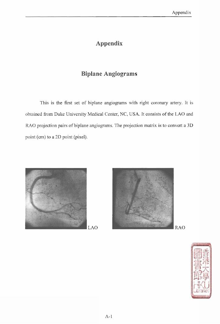
Appendix
Appendix
Biplane Angiograms
This is the first set of biplane angiograms with right coronary artery. It is
obtained from Duke University Medical Center, NC, USA. It consists of the LAO and
RAO projection pairs of biplane angiograms. The projection matrix is to convert a 3D
point (cm) to a 2D point (pixel).
A - l

Appendix
.
I
S
r
l
d
D
h g
3
:I ^
con
y
t
c
^ to
D
n
s
s
o
t
• 1
)
r
s
、
0
-1
X
c
t
l
s
r
i
A
o
a
t
c
m
1
t
1
h
i
m
thL
o
A
.tl
w
s
X
TJ
c
g
L
.01
m
^
r
a
rc
p
grN
比
.
¾ter
,
T
i
n
n
s
.
3
c
n
'
e
carr
a
n
l
s
g
r
1M
c
o
• 1
. IX
.>lld
g
b
仏
a
n
f
v
[
a
0
A-
e
•
过
.
l
t
y
§
叫
s 2
w
ix
ndwbicp
議
u
n
i
M
.mt
c
T-
s
o
s
e
i
r
F
e
k
m
)
k
u
p
D
D
n
2
s
1
o
a
1
m ti o
s
o
X
t
w
f
r
.
J
e
力
T
n
e
d
p
l
-
o
(
c
m
.
a
l⑷
n
t
h
l
A
o
i
o
R
p
A-2

Appendix
Multislice MR Images
This is the first set of multislice M R images with a brain tumor. It is obtained
from Image Processing Group at Guy's Hospital, London, U.K. It consists of 74 slices.
The pixel size is 0.898mm x 0.898mm. The slice thickness is 0.8mm.
A-3

slice 05
slice 07
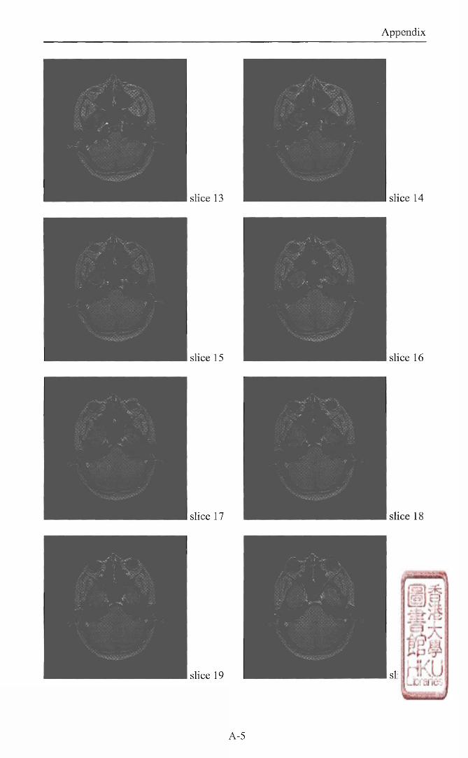
slice 13
slice 15
slice 17
slice 19
A-5

slice 23

Appendix
slice 29
slice 31
slice
si i r e
slice 30
slice 32
slice 34
slice 36
A-7
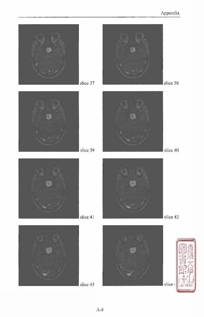
Appendix
slice 41 slice 42
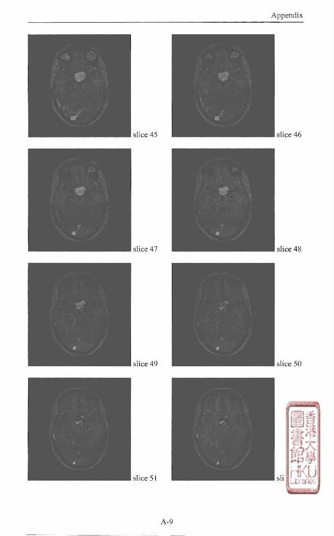
Appendix
slice 45
slice 47
slice 49
sl ice SI
slice 46
slice 48
slice 50
slice 52
A-9
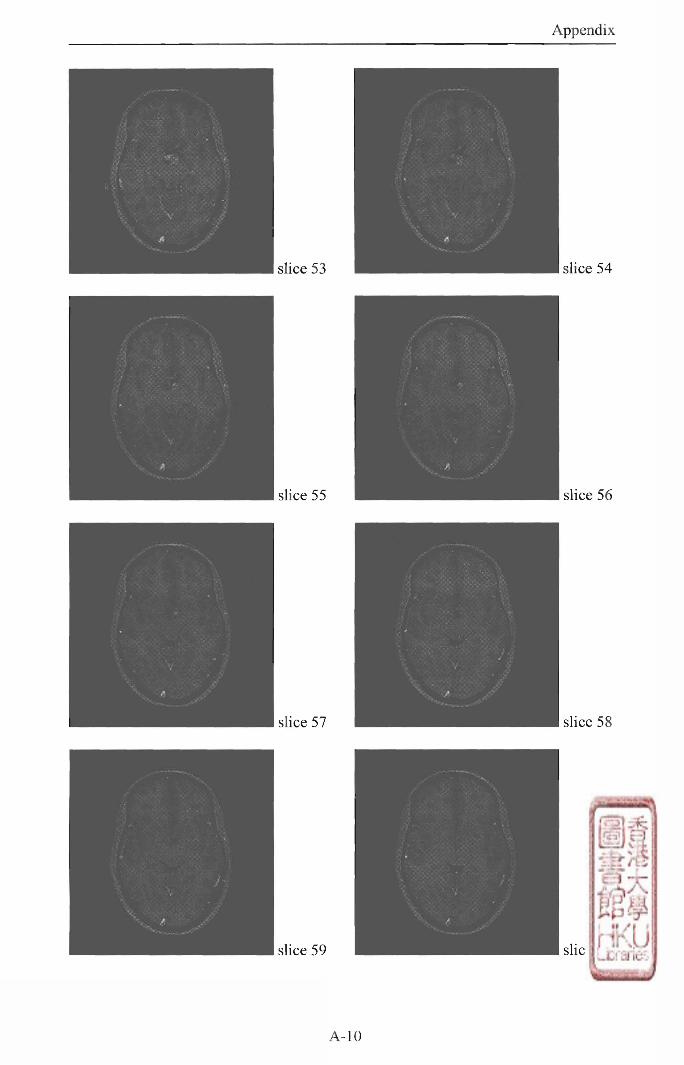
Appendix
slice 53
slice 55
slice 57
sl ice SQ
slice 54
slice 56
slice 58
slice 60
A-10

Appendix
slice 67 slice 68

slice 69
slice 71
slice 73
A-

Appendix
This is the second set of multislice M R images with a brain tumor. It is
obtained from Department of Radiology at Kwong Wah Hospital, Kowloon, Hong
Kong. It consists of 15 slices. The pixel size is 0.977mm x 0.977mm. The slice
thickness is 3mm.
slice 01 slice 02
slice 03 slice 04
slice 05 slice 06
A-13
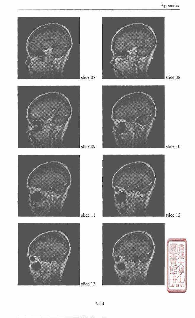
Appendix
slice 07 slice 08
slice
1 slice 12
slice 13 slice 14

3 1) JUL 2004 L Appendix
slice 15
A-15