University of São PauloInstitute of Mathematics and Statistics

Bachelor of Computer Science

Hash Functions and Hash Tables

Breno Helfstein Moura

Final Essaymac0499 — Capstone Project

Program: Computer ScienceAdvisor: José Coelho de Pina Junior

São PauloDecember 10th, 2019

Resumo

Breno Helfstein Moura. Funções e Tables de Hash. Monogra�a (Bacharelado). Instituto deMatemática e Estatística, Universidade de São Paulo, São Paulo, 2019.

Este trabalho de conclusão de curso trata de um dos mais fascinantes e úteis conceitos emciência da computação: funções de hash e tabelas de hash. O texto está organizado em trêspartes principais:

• Funções de Hash

• Tabelas de Hash

• Aplicações

Funções de hash é uma ideia importante em ciência da computação e vai muito além deseu uso em tabelas de hash. Nesse texto são descritas algumas das ideias que Donald Knuthapresentou em seu livro inspirador, The Art of Computer programming, Vol. 3 (Knuth, 1973).Estimamos a qualidade de funções de hash através de algumas métricas conhecidas.

Tabelas de hash é uma das mais usadas estruturas de dados em programação. Indicamosos componentes de tabelas de hash em que funções de hash têm um papel primordial. De-screvemos várias das implementações clássicas dessa estrutura; cada uma apropriada paraum determinado cenário.

Por �m, descrevemos algumas aplicações de funções e tabelas de hash em problemas recor-rentes em ciência da computação. Entre as aplicações está o algoritmo Rabin-Karp para buscade padrão em textos que utiliza hashing e um algoritmo e�ciente para identi�car isomor�smoem árvores utilizando funções de hash.

Espero que esse trabalho seja tão divertido de ler quanto foi para escrever!

Obs: O idioma escolhido para o trabalho foi o inglês devido a muitos termos que se referem ahashing estarem nesse idoma.

Palavras-chave: Hash. Hashing. Function. Maps. Dictionaries. Symbol Tables

Abstract

Breno Helfstein Moura. Hash Functions and Hash Tables. Capstone Project Report (Bach-elor). Institute of Mathematics and Statistics, University of São Paulo, São Paulo, 2019.

This text deals with one of the most fascinating and useful concepts in Computer Science,which are hash functions and hash tables. It is organized in three main topics:

• Hash functions

• Hash tables

• Applications

Hash functions is a key tool in Computer Science, its applications goes far beyond its usein hash tables. In this text it is presented some of the ideas Donald Knuth described in hisinspiring book, The Art of Computer programming, Vol. 3 (Knuth, 1973), and we apply somemetrics in order to estimate the quality of a hash function.

Hash tables is one of the most used data structures in computer programming. We presentthe constituents parts of a hash table, in which hash functions have a prominent role, andshow some of the classic implementations of this data structure; each one particularly usefulin a speci�c scenario.

Finally, we describe some applications of hash functions and hash tables in every day com-puter science problems. Among the algorithms shown there are Rabin-Karp, a string searchalgorithm that uses hashing and a solution to identify isomorphism on trees using hashingfunctions.

I hope this is as fun to read for you as it was for me to write!

Keywords: Hash. Hashing. Function. Maps. Dictionaries. Symbol Tables

v

Contents

1 Introduction 1

2 Hash Functions 52.1 De�nition . . . . . . . . . . . . . . . . . . . . . . . . . . . . . . . . . . . 62.2 Division and Multiplicative Methods . . . . . . . . . . . . . . . . . . . . 72.3 Hashing Strings . . . . . . . . . . . . . . . . . . . . . . . . . . . . . . . . 82.4 Quality of Hash Functions . . . . . . . . . . . . . . . . . . . . . . . . . . 9

3 Hash Tables 153.1 No collision open addressing hash table . . . . . . . . . . . . . . . . . . 173.2 Open addressing . . . . . . . . . . . . . . . . . . . . . . . . . . . . . . . . 183.3 Linear Probing . . . . . . . . . . . . . . . . . . . . . . . . . . . . . . . . . 193.4 Quadratic Probing . . . . . . . . . . . . . . . . . . . . . . . . . . . . . . . 213.5 Double Hashing . . . . . . . . . . . . . . . . . . . . . . . . . . . . . . . . 223.6 Robin Hood Hashing . . . . . . . . . . . . . . . . . . . . . . . . . . . . . 223.7 Cuckoo Hashing . . . . . . . . . . . . . . . . . . . . . . . . . . . . . . . . 253.8 Coalesced Hashing . . . . . . . . . . . . . . . . . . . . . . . . . . . . . . 273.9 Chaining hashing . . . . . . . . . . . . . . . . . . . . . . . . . . . . . . . 293.10 Simple Chaining Hashing Algorithm . . . . . . . . . . . . . . . . . . . . 303.11 Move to front . . . . . . . . . . . . . . . . . . . . . . . . . . . . . . . . . 313.12 How to delete an entry . . . . . . . . . . . . . . . . . . . . . . . . . . . . 323.13 When to resize an array . . . . . . . . . . . . . . . . . . . . . . . . . . . . 333.14 Open Addressing vs Chaining Hashing . . . . . . . . . . . . . . . . . . . 33

4 Applications 354.1 3-sum problem . . . . . . . . . . . . . . . . . . . . . . . . . . . . . . . . . 354.2 Rabin-Karp . . . . . . . . . . . . . . . . . . . . . . . . . . . . . . . . . . . 374.3 Complete tripartite graph . . . . . . . . . . . . . . . . . . . . . . . . . . . 404.4 Hashing trees to check for isomorphism . . . . . . . . . . . . . . . . . . . 40

vi

5 Final Remarks 43

References 45

1

Chapter 1

Introduction

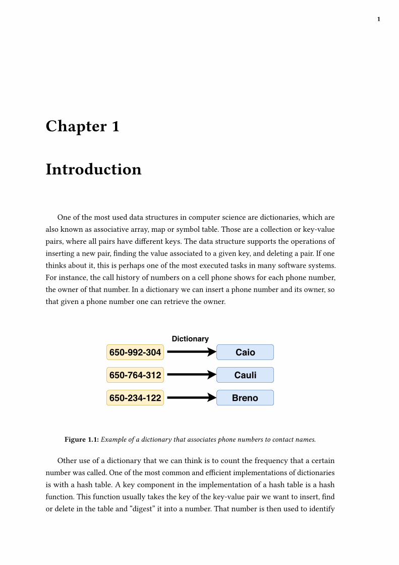
One of the most used data structures in computer science are dictionaries, which arealso known as associative array, map or symbol table. Those are a collection or key-valuepairs, where all pairs have di�erent keys. The data structure supports the operations ofinserting a new pair, �nding the value associated to a given key, and deleting a pair. If onethinks about it, this is perhaps one of the most executed tasks in many software systems.For instance, the call history of numbers on a cell phone shows for each phone number,the owner of that number. In a dictionary we can insert a phone number and its owner, sothat given a phone number one can retrieve the owner.

650-992-304

650-764-312

650-234-122

Caio

Cauli

Breno

Dictionary

Figure 1.1: Example of a dictionary that associates phone numbers to contact names.

Other use of a dictionary that we can think is to count the frequency that a certainnumber was called. One of the most common and e�cient implementations of dictionariesis with a hash table. A key component in the implementation of a hash table is a hashfunction. This function usually takes the key of the key-value pair we want to insert, �ndor delete in the table and “digest” it into a number. That number is then used to identify

2

1 | INTRODUCTION

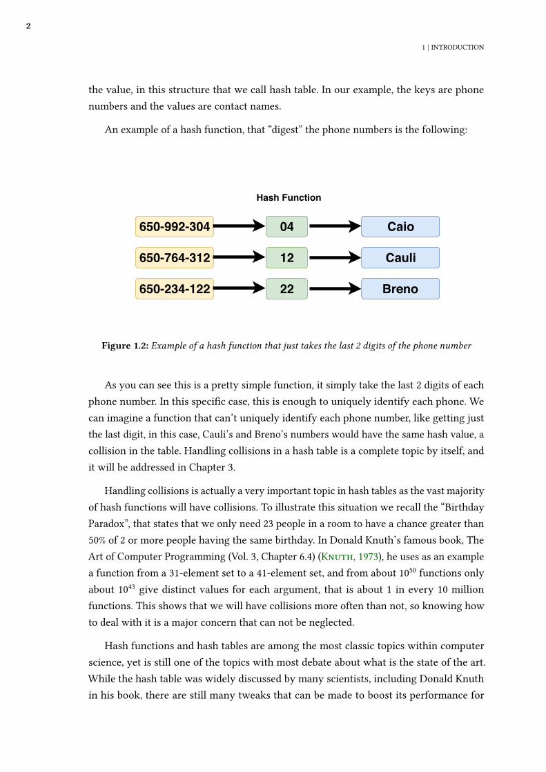
the value, in this structure that we call hash table. In our example, the keys are phonenumbers and the values are contact names.

An example of a hash function, that “digest” the phone numbers is the following:

650-992-304

650-764-312

650-234-122

Caio

Cauli

Breno

Hash Function

04

12

22

Figure 1.2: Example of a hash function that just takes the last 2 digits of the phone number

As you can see this is a pretty simple function, it simply take the last 2 digits of eachphone number. In this speci�c case, this is enough to uniquely identify each phone. Wecan imagine a function that can’t uniquely identify each phone number, like getting justthe last digit, in this case, Cauli’s and Breno’s numbers would have the same hash value, acollision in the table. Handling collisions in a hash table is a complete topic by itself, andit will be addressed in Chapter 3.

Handling collisions is actually a very important topic in hash tables as the vast majorityof hash functions will have collisions. To illustrate this situation we recall the “BirthdayParadox”, that states that we only need 23 people in a room to have a chance greater than50% of 2 or more people having the same birthday. In Donald Knuth’s famous book, TheArt of Computer Programming (Vol. 3, Chapter 6.4) (Knuth, 1973), he uses as an examplea function from a 31-element set to a 41-element set, and from about 1050 functions onlyabout 1043 give distinct values for each argument, that is about 1 in every 10 millionfunctions. This shows that we will have collisions more often than not, so knowing howto deal with it is a major concern that can not be neglected.

Hash functions and hash tables are among the most classic topics within computerscience, yet is still one of the topics with most debate about what is the state of the art.While the hash table was widely discussed by many scientists, including Donald Knuthin his book, there are still many tweaks that can be made to boost its performance for

1 | INTRODUCTION

3

speci�c use cases. One great example is F14, an open-source memory e�cient hash tableby Facebook (Facebook, 2019).

An example of lack of consensus in this area are the di�erent hash functions and hashtables built-in implementations in di�erent languages. There is no clear consensus onhow to decide the size of a hash table, what are the trade-o�s of the collision-resolutionalgorithms or even what de�nes a good hash function. Hopefully, we got years of researchon the topic to study and present a view on the subject, and that is what is presentedthroughout this undergraduate thesis.

It’s important to notice that during this thesis we will present code snippets of im-plementations, all of them are in C++14 and can be compiled with the following com-mand:

g++ -std=c++14 -Wall -Wshadow -O2 code.cpp -o code

5

Chapter 2

Hash Functions

Outside computer science, the word “hash” in the English language means to “chop” orto “mix” something. This meaning is entirely related to what hash functions are supposedto do. Hash functions are functions that are used to map data of an arbitrary size to dataof a �xed size (Wikipedia, 2019c).

They have wide applications in computer science, being used in information and datasecurity, compilers, distributed systems and hardcore algorithms. In this chapter we �rstde�ne and explain the basics of a hash function, then we give an intuition on some metricsthat tries to capture the idea of what is expected of a good hash function, as discussed inthe famous “Red Dragon Book” (Aho et al., 1986) along with some reproduction of knownresults in the area.

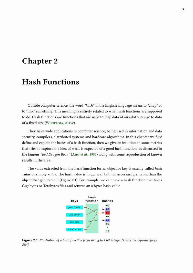
The value extracted from the hash function for an object or key is usually called hashvalue or simply value. The hash value is in general, but not necessarily, smaller than theobject that generated it (Figure 2.1). For example, we can have a hash function that takesGigabytes or Terabytes �les and returns an 8 bytes hash value.

hashfunctionkeys

John Smith

Lisa Smith

Sam Doe

Sandra Dee

hashes

00

01

02

03

04

05

:

15

Figure 2.1: Illustration of a hash function from string to 4 bit integer. Source: Wikipedia, JorgeStol�

6

2 | HASH FUNCTIONS

2.1 De�nition

A hash function over a set X is a function H that takes an element x in X and associatesto x an integer H (x) in the interval [0, M), for some integer M . In symbols

H ∶ X → [0, M)

When dealing with hash tables, X is the set of possible keys and M is the size of the table,which is usually just an array. Moreover, we saw earlier that hash functions are usuallymore useful when |X | > M . This is the same de�nition used by Donald Knuth (Knuth,1973) and some articles (Celis, 1986). This de�nition makes sense for our purpose becausewe will be talking mostly about hash functions used in hash tables. In that case we wantintegers that will be indexes in an array (as we will see later on). In other cases we maysee hash values as strings, like for when we hash a string for password storage or whenwe use a hash function in �les for checking integrity (for when we are checking if two�les are the same). For the goal of this text we will not cover those functions, but it isimportant to notice that strings can also be easily associated to integers if we just look attheir bytes.

For our purpose we are looking for a hash function that performs well for the con-struction of hash tables. Ideally, these functions should be fast to compute and minimizethe number of collisions. Depending on our goals we might want a di�erent metric, forcheck-sums for example we may want a function that is very sensible to changes, andfor passwords one that is very hard to �nd its inverse, those are so called cryptographicfunctions. For some collision resolution techniques, as we will see later, we may also wantthat the hash function disperse the values well too. Intuitively, a hash function shouldlook like a random function having a given key as seed.

As written in Knuth’s book, we know that it is theoretically impossible to create a hashfunction that generates true random data from non random data in actual �le, but we cando pretty close to that or in some cases, even fewer collision than an uniformly randomfunction. Knuth describes two speci�c methods for simple hash function, named divisionhashing and multiplicative hashing techniques. As the name suggests, the �rst is based ondivision operation and the latter on multiplication operation.

2.2 | DIVISION AND MULTIPLICATIVE METHODS

7

2.2 Division and Multiplicative Methods

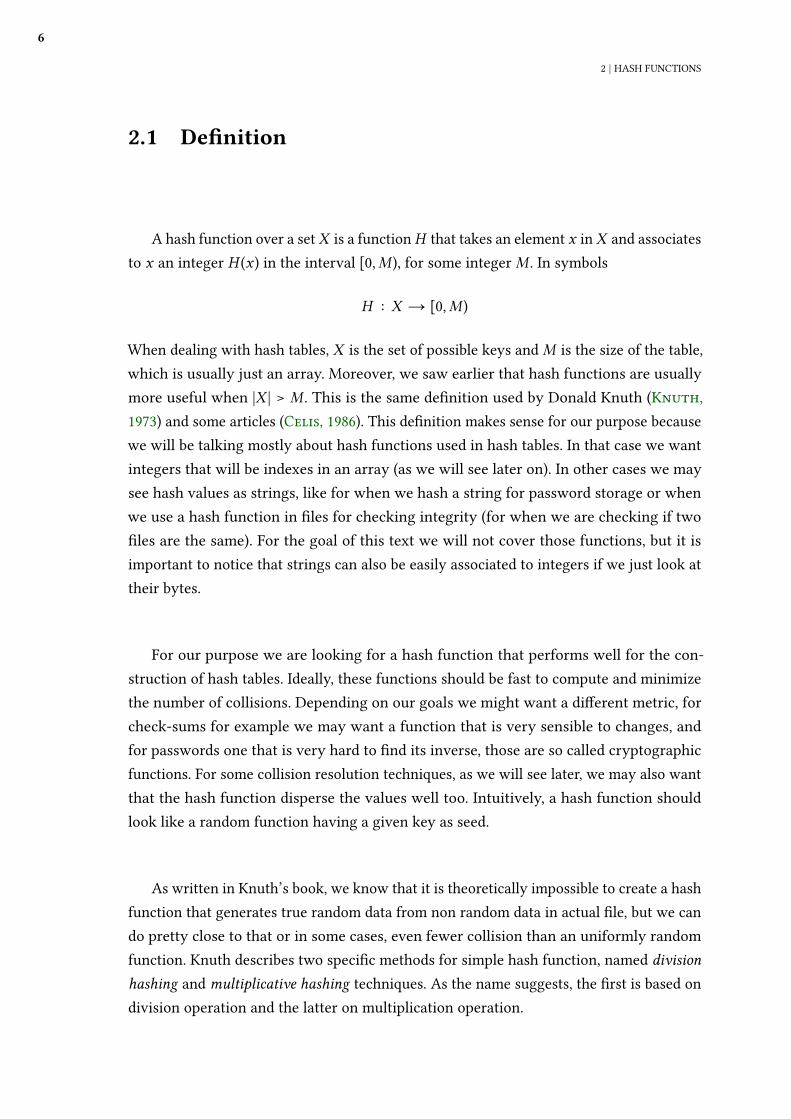
The division hashing method maps an integer X associated to the data to its remaindermodulo an integer M . Supposing we can represent the data as a non negative integer X ,the division hashing would be to choose a value M and the hashing function would be Xmod M . The code would look as following:

1 unsigned int d i v i s i o n H a s h i n g ( unsigned int X , unsigned int M ) {

2 return X % M ;

3 }

A good hash function combines number theory, statistics and engineering and ingeneral, large prime numbers tend to be a good value to M , to avoid unwanted patterns orrepetitions. One great example of this is if M is even, then the parity of hash value of Xwill match the parity of X (which will cause a bad distribution).

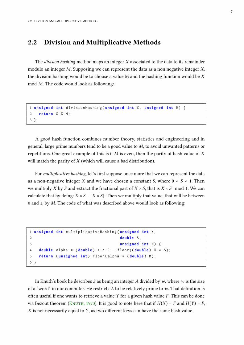
For multiplicative hashing, let’s �rst suppose once more that we can represent the dataas a non-negative integer X and we have chosen a constant S, where 0 < S < 1. Thenwe multiply X by S and extract the fractional part of X × S, that is X × S mod 1. We cancalculate that by doing: X × S − ⌊X × S⌋. Then we multiply that value, that will be between0 and 1, by M . The code of what was described above would look as following:

1 unsigned int m u l t i p l i c a t i v e H a s h i n g ( unsigned int X ,

2 double S ,

3 unsigned int M ) {

4 double alpha = ( double ) X * S - floor (( double ) X * S ) ;

5 return ( unsigned int ) floor ( alpha * ( double ) M ) ;

6 }

In Knuth’s book he describes S as being an integer A divided by w , where w is the sizeof a “word” in our computer. He restricts A to be relatively prime to w . That de�nition isoften useful if one wants to retrieve a value Y for a given hash value F . This can be donevia Bezout theorem (Knuth, 1973). It is good to note here that if H (X ) = F and H (Y ) = F ,X is not necessarily equal to Y , as two di�erent keys can have the same hash value.

8

2 | HASH FUNCTIONS

2.3 Hashing Strings

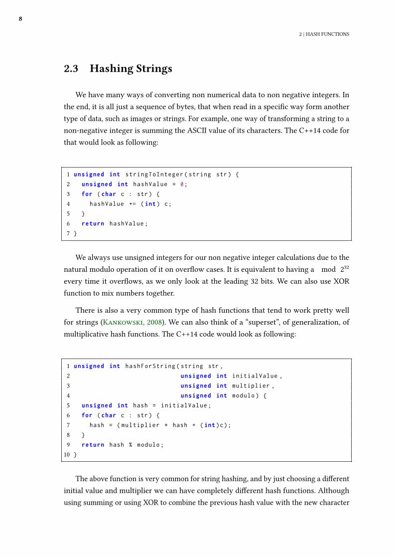
We have many ways of converting non numerical data to non negative integers. Inthe end, it is all just a sequence of bytes, that when read in a speci�c way form anothertype of data, such as images or strings. For example, one way of transforming a string to anon-negative integer is summing the ASCII value of its characters. The C++14 code forthat would look as following:

1 unsigned int s t r i n g T o I n t e g e r ( string str ) {

2 unsigned int hashValue = 0 ;

3 for ( char c : str ) {

4 hashValue += ( int ) c ;

5 }

6 return hashValue ;

7 }

We always use unsigned integers for our non negative integer calculations due to thenatural modulo operation of it on over�ow cases. It is equivalent to having a mod 2

32

every time it over�ows, as we only look at the leading 32 bits. We can also use XORfunction to mix numbers together.

There is also a very common type of hash functions that tend to work pretty wellfor strings (Kankowski, 2008). We can also think of a “superset”, of generalization, ofmultiplicative hash functions. The C++14 code would look as following:

1 unsigned int h a s h F o r S t r i n g ( string str ,

2 unsigned int initialValue ,

3 unsigned int multiplier ,

4 unsigned int modulo ) {

5 unsigned int hash = i n i t i a l V a l u e ;

6 for ( char c : str ) {

7 hash = ( m u l t i p l i e r * hash + ( int ) c ) ;

8 }

9 return hash % modulo ;

10 }

The above function is very common for string hashing, and by just choosing a di�erentinitial value and multiplier we can have completely di�erent hash functions. Althoughusing summing or using XOR to combine the previous hash value with the new character

2.4 | QUALITY OF HASH FUNCTIONS

9

usually don’t provide much di�erence, with XOR operation we do not need to worry aboutover�ow. Some values are of known hash functions, for example with multiplier = 33 andinitialValue = 5381 generates Bernstein hash djb2 (Bernstein, 1991) or multiplier = 31

and initialValue = 0 generates Kernighan and Ritchie’s hash (Kernighan and Ritchie,1988). Those are famous functions and their values are not chosen randomly, as there aresome factors that maximize the chance of producing a good hash function, where goodmeans low collision rate and fast computation. Those factors are:

• The multiplier should be bigger than the size of the alphabet, in our case usually26 for English words or 256 for ASCII. That is the case because if it is smaller wecan have wrong matches easier. For example, suppose that multiplier = 10 andinitialValue = 0, we have H (′ABA′) = H (′AAK ′

) = 7225 before taking the modulooperation.

• The multiplication by the multiplier should be easy to compute with simple opera-tions, such as bitwise operations and adding. That is quite intuitive as we want ahash function that is fast to calculate.

• The multiplier should be coprime with the modulo. That is because otherwise wewill “cycle” hashes at a greater rate than the modulo (We can use some modulararithmetic to prove that). Usually prime numbers tend to be good multipliers.

2.4 Quality of Hash Functions

Now that we know some good templates for producing hash functions let us try to �nda concrete metric or formula that measures the quality of a hash function. Fortunately, thefamous book Compilers: Principles, Techniques, and Tools, also known as “Red DragonBook” (Aho et al., 1986), has already proposed a quantity to measure the quality of a hashfunction. This quantity is given by:

m−1

∑

j=0

bj(bj + 1)/2

(n/2m)(n + 2m − 1)

,

where n is the number of keys, m is the number of total slots and bj is the number ofkeys in the j-th slot. The intuition for the numerator is that it represents the number ofoperations we will need to perform to �nd each element of the table. For example, we need1 operation to �nd the �rst element, 2 to �nd the second, and so on. That means that wewill end up with an arithmetic progression. We know that a hash function that distributesthe keys according to an uniformly random distribution has expected bucket size of n/m,

10

2 | HASH FUNCTIONS

so we can calculate that the expected value of the numerator formula is (n/2m)(n + 2m − 1).So that gives us a ratio of collisions (thinking just about operations to access a value) of“our” hash function with an “ideal” function. That means that a value close to 1.00 of theabove formula is good, and values below 1.00 means that we had less collisions than anuniformly distributed random function.

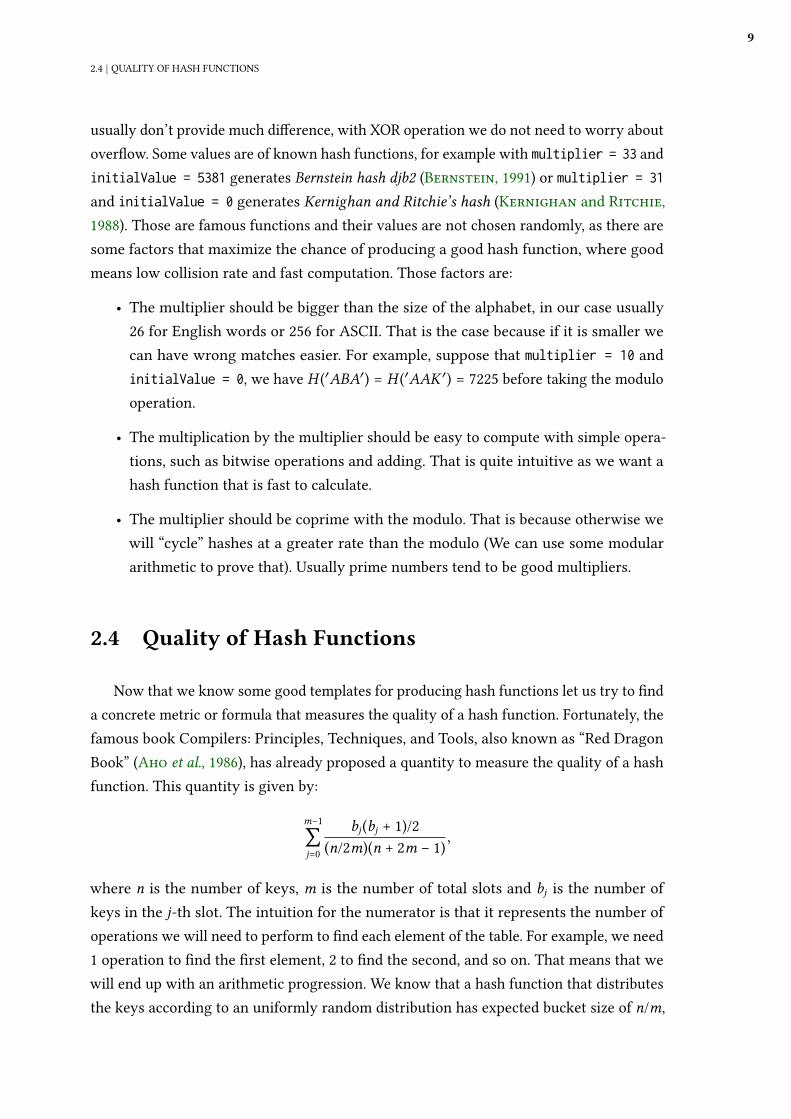
For common data as the ones in Dragon Book and Strchr website (Kankowski, 2008)some tests with the previously cited hash functions were performed.

Figure 2.2: Functions tested against a “small” table

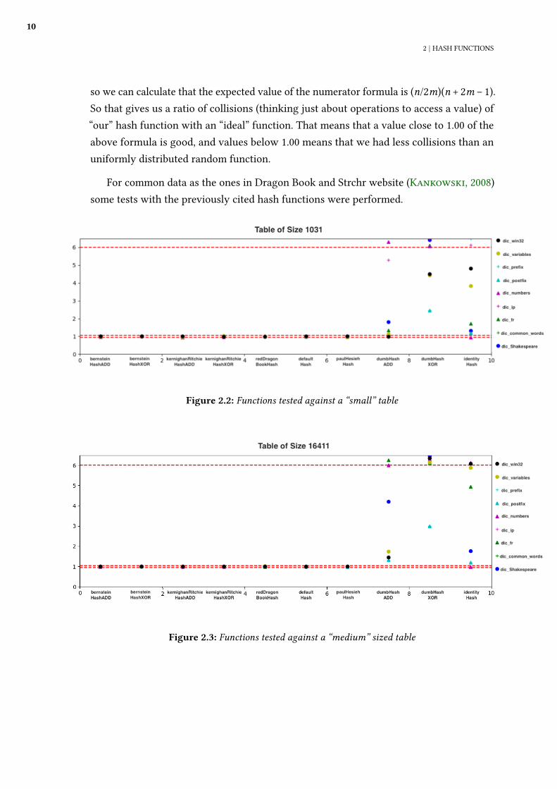
Figure 2.3: Functions tested against a “medium” sized table

2.4 | QUALITY OF HASH FUNCTIONS

11

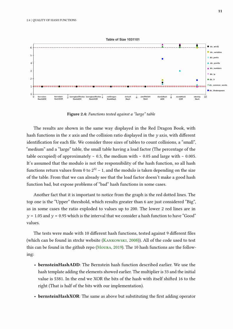
Figure 2.4: Functions tested against a “large” table

The results are shown in the same way displayed in the Red Dragon Book, withhash functions in the x axis and the collision ratio displayed in the y axis, with di�erentidenti�cation for each �le. We consider three sizes of tables to count collisions, a “small”,“medium” and a “large” table, the small table having a load factor (The percentage of thetable occupied) of approximately ∼ 0.5, the medium with ∼ 0.05 and large with ∼ 0.005.It’s assumed that the modulo is not the responsibility of the hash function, so all hashfunctions return values from 0 to 232 − 1, and the modulo is taken depending on the sizeof the table. From that we can already see that the load factor doesn’t make a good hashfunction bad, but expose problems of “bad” hash functions in some cases.

Another fact that it is important to notice from the graph is the red dotted lines. Thetop one is the “Upper” threshold, which results greater than 6 are just considered “Big”,as in some cases the ratio exploded to values up to 200. The lower 2 red lines are iny = 1.05 and y = 0.95which is the interval that we consider a hash function to have “Good”values.

The tests were made with 10 di�erent hash functions, tested against 9 di�erent �les(which can be found in strchr website (Kankowski, 2008)). All of the code used to testthis can be found in the github repo (Moura, 2019). The 10 hash functions are the follow-ing:

• bernsteinHashADD: The Bernstein hash function described earlier. We use thehash template adding the elements showed earlier. The multiplier is 33 and the initialvalue is 5381. In the end we XOR the bits of the hash with itself shifted 16 to theright (That is half of the bits with our implementation).

• bernsteinHashXOR: The same as above but substituting the �rst adding operator

12

2 | HASH FUNCTIONS

by the XOR operation.

• kernighanRitchieHashADD The Kernighan and Ritchie Hash function describedearlier. We use the given hash template adding the elements. The multiplier is 31and the initial value is 0.

• kernighanRitchieHashXOR The same as above but substituting the �rst addingoperator by the XOR operation.

• redDragonBookHash The hash function tested in the Red Dragon Book. It isdescribed as x65599 in the book.

• defaultHash The default hash function of C++ standard template library.

• paulHesiehHash A fast hash function described by Paul Hesieh (Hesieh, 2004). Itis fast to calculate and more complex than Knuth multiplicative or division Hashing.

• dumbHashADD A hash function that simply add all characters.

• dumbHashXOR A hash function that simply XOR all characters.

• identityHash A hash function that takes the �rst 4 bytes of the string.

We have a variety of hash functions, with all being considered “fast” hash functions.The �les tested include common words in English and french, strings of some IP values,numbers, common variable names and words with common pre�x and su�x.

First, we can notice from those graphs that changing the ADD function to XOR doesn’tmake a good multiplicative hash function bad. Both are actually “Equivalent” given thatwe are also multiplying the values. For dumbHashADD and dumbHashXOR we can see cleardi�erences, with dumbHashXOR being clearly worse. This can be explained by the cancellationproperty of XOR. We can see this example on the hash of this IP below:

dumbHashXOR(’168.1.1.0’) = dumbHashXOR(’168.2.2.0’) = dumbHashXOR(’124.6.8.0’)

We can see that many di�erent IPs have the same hash value. More than that, XORdon’t increase the number of bits, so all the hashes will be of just 1 byte.

We can also notice that “identity” hash is good or perfect in some cases. One obviouscase that “identity” function works perfectly is for numbers as we will have 0 collisions.Some languages, like Python 3, use the identity function to calculate hash for integers,as it is very fast and produces no collisions. But we can see that for other cases, such ascommon pre�x, it works terrible as we just get the �rst 4 bytes.

The most common multiplicative hash functions tend to work similarly well, beingreasonably close to an uniformly random function (that is our “ideal” hash function) in all

2.4 | QUALITY OF HASH FUNCTIONS

13

cases.

As we can see, we don’t need a lot of complexity to make a good hash function for ahash table. We have some functions working better for some speci�c case, like identityfunction working well for numbers, but general functions already work well enough.

It is important to note here that hash function is a very vast topic, and here wejust covered hash functions related to hash tables. Hash functions have applicationsin distributed systems (consistent hashing), database indexing, caching, compilers (RedDragon Book) and cryptography. Each application has di�erent requirements and makesome hash functions better than others.

15

Chapter 3

Hash Tables

Hash tables or hash maps is one of the most used applications of hash functions. It isactually so used in computer science that is almost impossible to talk about one withoutmentioning the other. This data structure consists in associating a key to a value in a table.That is, given a key, it can retrieve the value for it.

It is one of the possible, and many times considered the best, implementations of adictionary. It has to implement the insert, find and remove operations, that can be accessedfrom outside the dictionary. It usually implements a lot of other private methods.

This data structure is usually considered very useful among software engineers andcomputer scientists, although it usually has a linear worst case cost for retrieving, insertingand deleting a key-value pair. That is because hash tables usually have a constant averagecost for those operations.

Moreover, when talking about hash tables we have the problem of key collision, that iswhen two keys map to the same hash value. As we saw in the previous chapter, collisionsare more common than not, so collision resolution is a critical problem. To solve thatproblem, we have several techniques that involve di�erent trade-o�s. Those techniquesare usually divided into two main categories, open addressing and separate chaining.Other problem to consider regarding this data structure is when to resize the hash table,to minimize the chance of collision and the use o memory. For this last one we usuallyconsider a load factor, � , that is the ratio of keys with the available slots in the table.

16

3 | HASH TABLES

Also, hash tables can be easily abstracted to hash sets, commonly used to store a set ofelements and check whether an element is in the set. We can abstract hash sets to a hashtable always with an empty value. Hash sets are one of the common ways to implementsets in programming languages, like unordered_set from C++14.

It is also important to notice that hash tables have applications in di�erent areas ofcomputer science also, like compilers, caches and database indexing.

hashfunctionkeys

John Smith

Lisa Smith

Sandra Dee

buckets

00

01 521-8976

02 521-1234

03

: :

13

14 521-9655

15

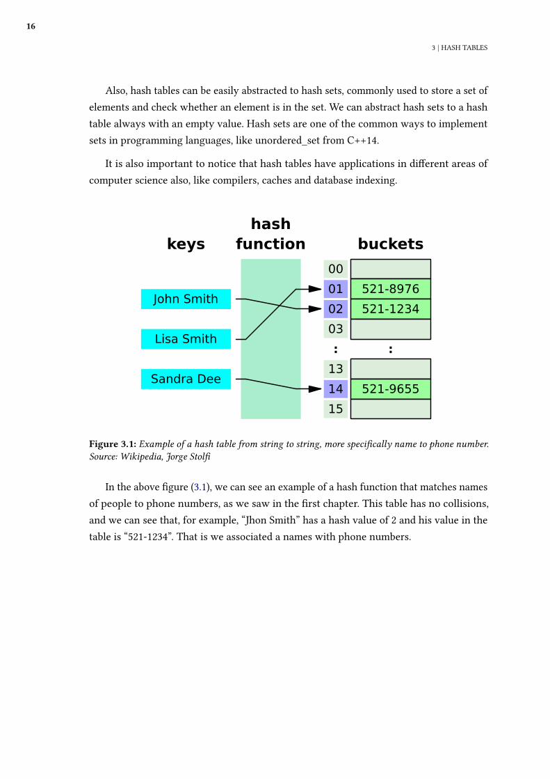
Figure 3.1: Example of a hash table from string to string, more speci�cally name to phone number.Source: Wikipedia, Jorge Stol�

In the above �gure (3.1), we can see an example of a hash function that matches namesof people to phone numbers, as we saw in the �rst chapter. This table has no collisions,and we can see that, for example, “Jhon Smith” has a hash value of 2 and his value in thetable is “521-1234”. That is we associated a names with phone numbers.

3.1 | NO COLLISION OPEN ADDRESSING HASH TABLE

17

3.1 No collision open addressing hash table

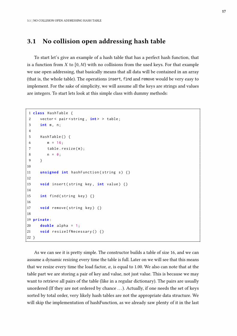
To start let’s give an example of a hash table that has a perfect hash function, thatis a function from X to [0, M) with no collisions from the used keys. For that examplewe use open addressing, that basically means that all data will be contained in an array(that is, the whole table). The operations insert, find and remove would be very easy toimplement. For the sake of simplicity, we will assume all the keys are strings and valuesare integers. To start lets look at this simple class with dummy methods:

1 class HashTable {

2 vector < pair < string , int > > table ;

3 int m , n ;

45 HashTable () {

6 m = 1 6 ;

7 table . resize ( m ) ;

8 n = 0 ;

9 }

1011 unsigned int h a s h F u n c t i o n ( string s ) {}

1213 void insert ( string key , int value ) {}

1415 int find ( string key ) {}

1617 void remove ( string key ) {}

1819 private :

20 double alpha = 1 ;

21 void r e s i z e I f N e c e s s a r y () {}

22 }

As we can see it is pretty simple. The constructor builds a table of size 16, and we canassume a dynamic resizing every time the table is full. Later on we will see that this meansthat we resize every time the load factor, � , is equal to 1.00. We also can note that at thetable part we are storing a pair of key and value, not just value. This is because we maywant to retrieve all pairs of the table (like in a regular dictionary). The pairs are usuallyunordered (If they are not ordered by chance . . . ). Actually, if one needs the set of keyssorted by total order, very likely hash tables are not the appropriate data structure. Wewill skip the implementation of hashFunction, as we already saw plenty of it in the last

18

3 | HASH TABLES

chapter, so we will go right in for the implementation of insert:

1 void insert ( string key , int value ) {

2 r e s i z e I f N e c e s s a r y () ;

3 unsigned int idx = h a s h F u n c t i o n ( key ) ;

4 table [ idx ] = pair < string , int >( key , value ) ;

5 n ++;

6 }

That is pretty simple, that is mostly because we will assume that we will never have acollision, so we just put the key on the position returned by the hash function. The methodfind is implemented as following:

1 int find ( string key ) {

2 unsigned int idx = h a s h F u n c t i o n ( key ) ;

3 if ( table [ idx ]. first == key )

4 return table [ idx ]. second ;

5 return 0 ;

6 }

Also very simple, we always know the value will be in position returned by idx. Theremove will be of the same simplicity, as following:

1 void remove ( string key ) {

2 unsigned int idx = h a s h F u n c t i o n ( key ) ;

3 table [ idx ]. first = pair < string , int >( " " , 0 ) ;

4 n - -;

5 }

Here we make the assumption that an empty position has an empty string. We couldalso carry a boolean, usually called a tombstone, to check if the position is occupied or not.If the hash function is perfect, than the insert, �nd and delete operations can be performedin constant time and linear space.

3.2 Open addressing

We can de�ne open addressing in a general way as a hash table algorithm where thedata always stay within the same vector. So, in the case of a collision, we need to de�ne a

3.3 | LINEAR PROBING

19

systematic way to traverse the table. The sequence of elements we need to traverse whenwe have a collision is called “Probe sequence”. With that our hash function would changeto the following:

ℎ(x, i)

, where x is our key and i is the probe sequence number. So every time we have a collisionin ℎ(x, i) we can simply go to ℎ(x, i + 1). Given that, lets look into some di�erent probesequences.

At the end of each section there will be auand adto indicate a summary of prosand cons.

3.3 Linear Probing

Linear probing is one of the most simple an practical probe sequences known. Theprobe sequence is basically:

ℎ(x, i) = (H (x) + i) mod M

, where M is the table size. That is a very simple probe sequence with not much secret onit. To implement the insert we can do the following:

1 void insert ( string key , int value ) {

2 r e s i z e I f N e c e s s a r y () ;

3 unsigned int idx = h a s h F u n c t i o n ( key ) ;

4 while ( table [ idx ] != pair < string , int >( " " , 0 ) )

5 idx = ( idx + 1 ) % m ;

6 table [ idx ] = pair < string , int >( key , value ) ;

7 n ++;

8 }

That assumes that pair<string, int>("", 0) is the empty position, and performsa linear search until it �nds one empty position to put the new (key, value) pair. Theimplementation of find is very similar:

20

3 | HASH TABLES

1 int find ( string key ) {

2 unsigned int idx = h a s h F u n c t i o n ( key ) ;

3 while ( table [ idx ] != pair < string , int >( " " , 0 ) ) {

4 if ( table [ idx ]. first == key )

5 return table [ idx ]. second ;

6 idx = ( idx + 1 ) % m ;

7 }

8 return 0 ; // Default value

9 }

It performs a linear search until it �nds the element. If the key is not found the functionreturns a default value, that in our case is 0.

For removal, we have the problem that we cannot leave “holes” in our table. That willbe discussed more in depth later on the section “How to delete an entry”. For now we willremove the element, and reinsert the key-value pairs that come right after it:

1 void remove ( string key ) {

2 unsigned int idx = h a s h F u n c t i o n ( key ) ;

3 while ( table [ idx ] != pair < string , int >( " " , 0 ) ) {

4 if ( table [ idx ]. first == key )

5 break ;

6 idx = ( idx + 1 ) % m ;

7 }

89 if ( table [ idx ]. first == key ) {

10 table [ idx ] = pair < string , int >( " " , 0 ) ;

11 vector < pair < string , int > > toRehash ;

12 int j = ( idx + 1 ) % m ;

13 while ( table [ j ] != pair < string , int >( " " , 0 ) ) {

14 toRehash . push_back ( table [ j ]) ;

15 table [ j ] = pair < string , int >( " " , 0 ) ;

16 j = ( j + 1 ) % m ;

17 }

18 for ( auto p : toRehash ) {

19 insert ( p . first , p . second ) ;

20 }

21 n - -;

22 }

23 }

With that, the three operations have linear time complexity in the worst case. As we

3.4 | QUADRATIC PROBING

21

saw, we know hash functions that are considered good, with a rate of collision very closeto an uniformly random function. Those functions will leave us with an expected constanttime complexity for those operations, and we will see later on that in practice it is muchfaster than linear access. Another great bene�t that linear probing has, specially whencompared to other collision resolution strategies, is locality and cache friendliness.

However linear probing has the problem of clustering, that is long chains of occupiedpositions. This generates a greater problem, as long chains are only expected to get longerand longer. This can get worse if the hash function is not too sensitive to changes, havinga lot of sequential hash values.

u It is easy to implement and cache friedly.

d It has problems with clustering.

3.4 Quadratic Probing

Another strategy for resolving collisions is quadratic probing. In this case, the probesequence can be de�ned as:

ℎ(x, i) = (H (x) + i2) mod M.

That solves the problem of having sequential hash values. The implementation of quadraticprobing is very similar to the implementation of linear probing, with the exception thatinstead of adding one for each step we can keep the initial value and add the square of acounter.

However, quadratic probing doesn’t solve the problem of clustering. Long chains arestill expected to get longer and longer, the only di�erence is that the positions that lead toa longer chain are better distributed in the table. Another thing to notice is that quadraticprobing has a worse locality and cache friendliness than linear probing.

u It is easy to implement and has less problems with clustering than linear probing.

d It is less cache friendly than linear probing and still has some clustering problems.

22

3 | HASH TABLES

3.5 Double Hashing

As we saw the two strategies above have the problem of clustering, due to the factthat the sequences are the same for all keys. For that reason double hashing is a verygood approach for open addressing. Double hashing probe sequence can be de�ned asfollowing:

ℎ(x, i) = (H1(x) + i ∗ H2(x)) mod M,

where H1 and H2 are two distinct hash functions. In that way not only the initial hashvalue will depend on x , but it’s probe sequence o�set (that is, the number of slots betweenℎ(x, i) and ℎ(x, i + 1)) will too. The implementation of double hashing is very similar toboth quadratic and linear probing, except that we sum a di�erent o�set.

These last three implementations of hash table give us linear time worst case complexityfor all operations and constant time expected time complexity under the simple uniformhashing assumption.

u It is harder to get collisions than linear probing and chaining hashing.

d It is less cache friendly than linear probing and requires 2 hash functions.

3.6 Robin Hood Hashing

Robin Hood Hashing is an optimization technique regarding collision resolution withopen addressing. It should be paired with Linear Probing, Quadratic Probing or DoubleHashing, but usually it is paired with linear probing due to it is good locality and cachefriendliness. It is basic is that it minimizes the distance of each key from its “home Slot”,that is, its initial hash value position. (Celis, 1986). Also, Robin Hood hashing is one ofthe few open addressing strategies to be built-in in hash tables of some languages, such asRust.

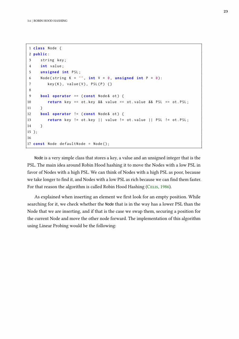
In order to minimize the distance from each key from its home slot, Robin Hoodhashing uses a concept that is called Probe Sequence Length, or PSL, of a key-value pair.The PSL of a key-value pair is the number of probes required to �nd that pair. For thatreason we need to de�ne a new class to store in our table, that we will call Node:

3.6 | ROBIN HOOD HASHING

23

1 class Node {

2 public :

3 string key ;

4 int value ;

5 unsigned int PSL ;

6 Node ( string K = " " , int V = 0 , unsigned int P = 0 ) :

7 key ( K ) , value ( V ) , PSL ( P ) {}

89 bool operator == ( const Node & ot ) {

10 return key == ot . key && value == ot . value && PSL == ot . PSL ;

11 }

12 bool operator != ( const Node & ot ) {

13 return key != ot . key || value != ot . value || PSL != ot . PSL ;

14 }

15 };

1617 const Node d e f a u l t N o d e = Node () ;

Node is a very simple class that stores a key, a value and an unsigned integer that is thePSL. The main idea around Robin Hood hashing it to move the Nodes with a low PSL infavor of Nodes with a high PSL. We can think of Nodes with a high PSL as poor, becausewe take longer to �nd it, and Nodes with a low PSL as rich because we can �nd them faster.For that reason the algorithm is called Robin Hood Hashing (Celis, 1986).

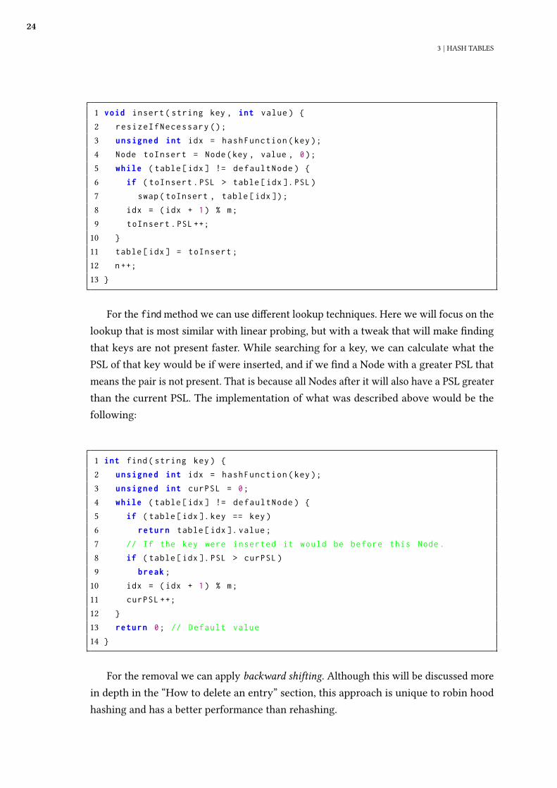
As explained when inserting an element we �rst look for an empty position. Whilesearching for it, we check whether the Node that is in the way has a lower PSL than theNode that we are inserting, and if that is the case we swap them, securing a position forthe current Node and move the other node forward. The implementation of this algorithmusing Linear Probing would be the following:

24

3 | HASH TABLES

1 void insert ( string key , int value ) {

2 r e s i z e I f N e c e s s a r y () ;

3 unsigned int idx = h a s h F u n c t i o n ( key ) ;

4 Node toInsert = Node ( key , value , 0 ) ;

5 while ( table [ idx ] != d e f a u l t N o d e ) {

6 if ( toInsert . PSL > table [ idx ]. PSL )

7 swap ( toInsert , table [ idx ]) ;

8 idx = ( idx + 1 ) % m ;

9 toInsert . PSL ++;

10 }

11 table [ idx ] = toInsert ;

12 n ++;

13 }

For the find method we can use di�erent lookup techniques. Here we will focus on thelookup that is most similar with linear probing, but with a tweak that will make �ndingthat keys are not present faster. While searching for a key, we can calculate what thePSL of that key would be if were inserted, and if we �nd a Node with a greater PSL thatmeans the pair is not present. That is because all Nodes after it will also have a PSL greaterthan the current PSL. The implementation of what was described above would be thefollowing:

1 int find ( string key ) {

2 unsigned int idx = h a s h F u n c t i o n ( key ) ;

3 unsigned int curPSL = 0 ;

4 while ( table [ idx ] != d e f a u l t N o d e ) {

5 if ( table [ idx ]. key == key )

6 return table [ idx ]. value ;

7 // If the key were inserted it would be before this Node .

8 if ( table [ idx ]. PSL > curPSL )

9 break ;

10 idx = ( idx + 1 ) % m ;

11 curPSL ++;

12 }

13 return 0 ; // Default value

14 }

For the removal we can apply backward shifting. Although this will be discussed morein depth in the “How to delete an entry” section, this approach is unique to robin hoodhashing and has a better performance than rehashing.

3.7 | CUCKOO HASHING

25

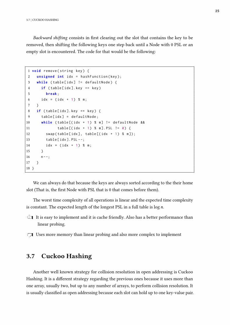
Backward shifting consists in �rst clearing out the slot that contains the key to beremoved, then shifting the following keys one step back until a Node with 0 PSL or anempty slot is encountered. The code for that would be the following:

1 void remove ( string key ) {

2 unsigned int idx = h a s h F u n c t i o n ( key ) ;

3 while ( table [ idx ] != d e f a u l t N o d e ) {

4 if ( table [ idx ]. key == key )

5 break ;

6 idx = ( idx + 1 ) % m ;

7 }

8 if ( table [ idx ]. key == key ) {

9 table [ idx ] = d e f a u l t N o d e ;

10 while ( table [( idx + 1 ) % m ] != d e f a u l t N o d e &&

11 table [( idx + 1 ) % m ]. PSL != 0 ) {

12 swap ( table [ idx ] , table [( idx + 1 ) % m ]) ;

13 table [ idx ]. PSL - -;

14 idx = ( idx + 1 ) % m ;

15 }

16 n - -;

17 }

18 }

We can always do that because the keys are always sorted according to the their homeslot (That is, the �rst Node with PSL that is 0 that comes before them).

The worst time complexity of all operations is linear and the expected time complexityis constant. The expected length of the longest PSL in a full table is log n.

u It is easy to implement and it is cache friendly. Also has a better performance thanlinear probing.

d Uses more memory than linear probing and also more complex to implement

3.7 Cuckoo Hashing

Another well known strategy for collision resolution in open addressing is CuckooHashing. It is a di�erent strategy regarding the previous ones because it uses more thanone array, usually two, but up to any number of arrays, to perform collision resolution. Itis usually classi�ed as open addressing because each slot can hold up to one key-value pair.

26

3 | HASH TABLES

For this explanation let’s assume that we are using two arrays. Cuckoo hashing requiresalso one hash function per array used, in our case two hash functions.

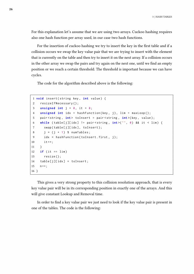
For the insertion of cuckoo hashing we try to insert the key in the �rst table and if acollision occurs we swap the key value pair that we are trying to insert with the elementthat is currently on the table and then try to insert it on the next array. If a collision occursin the other array we swap the pairs and try again on the next one, until we �nd an emptyposition or we reach a certain threshold. The threshold is important because we can havecycles.

The code for the algorithm described above is the following:

1 void insert ( string key , int value ) {

2 r e s i z e I f N e c e s s a r y () ;

3 unsigned int j = 0 , it = 0 ;

4 unsigned int idx = h a s h F u n c t i o n ( key , j ) , lim = maxLoop () ;

5 pair < string , int > toInsert = pair < string , int >( key , value ) ;

6 while ( table [ j ][ idx ] != pair < string , int >( " " , 0 ) && it < lim ) {

7 swap ( table [ j ][ idx ] , toInsert ) ;

8 j = ( j + 1 ) % numTables ;

9 idx = h a s h F u n c t i o n ( toInsert . first , j ) ;

10 it ++;

11 }

12 if ( it == lim )

13 resize () ;

14 table [ j ][ idx ] = toInsert ;

15 n ++;

16 }

This gives a very strong property to this collision resolution approach, that is everykey value pair will be in its corresponding position in exactly one of the arrays. And thiswill give constant Lookup and Removal time.

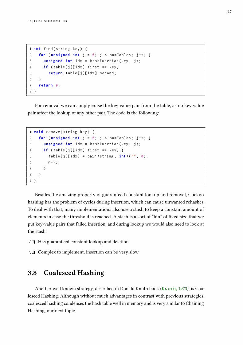
In order to �nd a key value pair we just need to look if the key value pair is present inone of the tables. The code is the following:

3.8 | COALESCED HASHING

27

1 int find ( string key ) {

2 for ( unsigned int j = 0 ; j < numTables ; j ++) {

3 unsigned int idx = h a s h F u n c t i o n ( key , j ) ;

4 if ( table [ j ][ idx ]. first == key )

5 return table [ j ][ idx ]. second ;

6 }

7 return 0 ;

8 }

For removal we can simply erase the key value pair from the table, as no key valuepair a�ect the lookup of any other pair. The code is the following:

1 void remove ( string key ) {

2 for ( unsigned int j = 0 ; j < numTables ; j ++) {

3 unsigned int idx = h a s h F u n c t i o n ( key , j ) ;

4 if ( table [ j ][ idx ]. first == key ) {

5 table [ j ][ idx ] = pair < string , int >( " " , 0 ) ;

6 n - -;

7 }

8 }

9 }

Besides the amazing property of guaranteed constant lookup and removal, Cuckoohashing has the problem of cycles during insertion, which can cause unwanted rehashes.To deal with that, many implementations also use a stash to keep a constant amount ofelements in case the threshold is reached. A stash is a sort of “bin” of �xed size that weput key-value pairs that failed insertion, and during lookup we would also need to look atthe stash.

u Has guaranteed constant lookup and deletion

d Complex to implement, insertion can be very slow

3.8 Coalesced Hashing

Another well known strategy, described in Donald Knuth book (Knuth, 1973), is Coa-lesced Hashing. Although without much advantages in contrast with previous strategies,coalesced hashing condenses the hash table well in memory and is very similar to ChainingHashing, our next topic.

28

3 | HASH TABLES

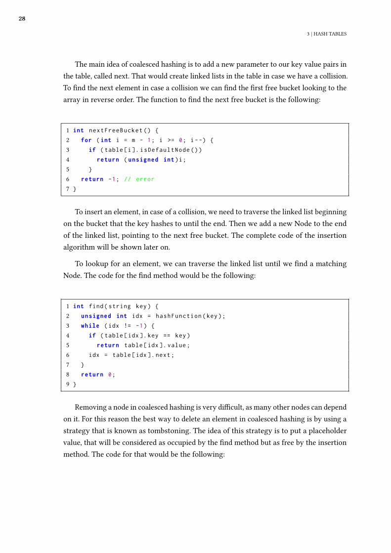
The main idea of coalesced hashing is to add a new parameter to our key value pairs inthe table, called next. That would create linked lists in the table in case we have a collision.To �nd the next element in case a collision we can �nd the �rst free bucket looking to thearray in reverse order. The function to �nd the next free bucket is the following:

1 int n e x t F r e e B u c k e t () {

2 for ( int i = m - 1 ; i >= 0 ; i - -) {

3 if ( table [ i ]. i s D e f a u l t N o d e () )

4 return ( unsigned int ) i ;

5 }

6 return -1 ; // error

7 }

To insert an element, in case of a collision, we need to traverse the linked list beginningon the bucket that the key hashes to until the end. Then we add a new Node to the endof the linked list, pointing to the next free bucket. The complete code of the insertionalgorithm will be shown later on.

To lookup for an element, we can traverse the linked list until we �nd a matchingNode. The code for the �nd method would be the following:

1 int find ( string key ) {

2 unsigned int idx = h a s h F u n c t i o n ( key ) ;

3 while ( idx != -1 ) {

4 if ( table [ idx ]. key == key )

5 return table [ idx ]. value ;

6 idx = table [ idx ]. next ;

7 }

8 return 0 ;

9 }

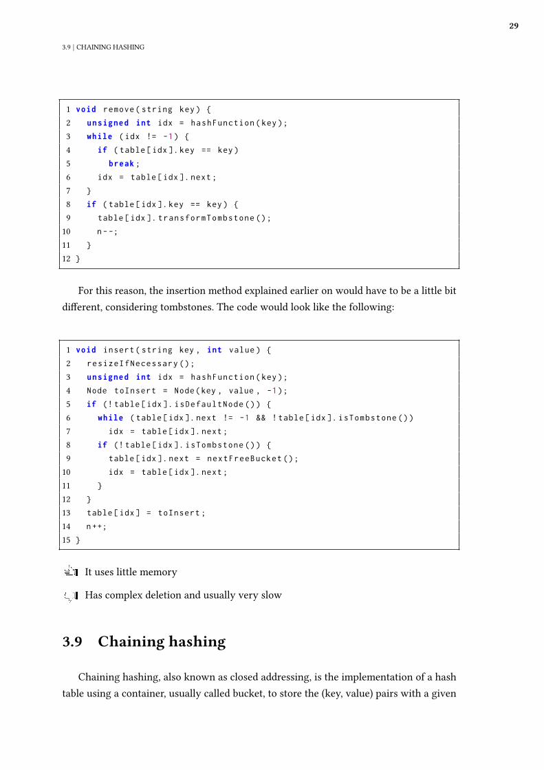
Removing a node in coalesced hashing is very di�cult, as many other nodes can dependon it. For this reason the best way to delete an element in coalesced hashing is by using astrategy that is known as tombstoning. The idea of this strategy is to put a placeholdervalue, that will be considered as occupied by the �nd method but as free by the insertionmethod. The code for that would be the following:

3.9 | CHAINING HASHING

29

1 void remove ( string key ) {

2 unsigned int idx = h a s h F u n c t i o n ( key ) ;

3 while ( idx != -1 ) {

4 if ( table [ idx ]. key == key )

5 break ;

6 idx = table [ idx ]. next ;

7 }

8 if ( table [ idx ]. key == key ) {

9 table [ idx ]. t r a n s f o r m T o m b s t o n e () ;

10 n - -;

11 }

12 }

For this reason, the insertion method explained earlier on would have to be a little bitdi�erent, considering tombstones. The code would look like the following:

1 void insert ( string key , int value ) {

2 r e s i z e I f N e c e s s a r y () ;

3 unsigned int idx = h a s h F u n c t i o n ( key ) ;

4 Node toInsert = Node ( key , value , -1 ) ;

5 if (! table [ idx ]. i s D e f a u l t N o d e () ) {

6 while ( table [ idx ]. next != -1 && ! table [ idx ]. i s T o m b s t o n e () )

7 idx = table [ idx ]. next ;

8 if (! table [ idx ]. i s T o m b s t o n e () ) {

9 table [ idx ]. next = n e x t F r e e B u c k e t () ;

10 idx = table [ idx ]. next ;

11 }

12 }

13 table [ idx ] = toInsert ;

14 n ++;

15 }

u It uses little memory

d Has complex deletion and usually very slow

3.9 Chaining hashing

Chaining hashing, also known as closed addressing, is the implementation of a hashtable using a container, usually called bucket, to store the (key, value) pairs with a given

30

3 | HASH TABLES

hash. On this implementation, each bucket of the table is a linked list, that will carry thekey value pair in our case. We deal with collisions with this implementation by adding anew node to the start of the list.

This implementation is considered simpler than open addressing, usually because theway of dealing with collisions is clearer. Also it is less system dependent if we considerperformance (as we saw one of the key advantages of open addressing is that it is cachefriendly). That is one of the key reasons that C++ uses chaining hashing for its defaultimplementation of unordered_hash (Austern, 2003a).

Below we will discuss an implementation of chaining hashing and just like in openaddressing at the end of each section there will be auand adto indicate a summaryof pros and cons.

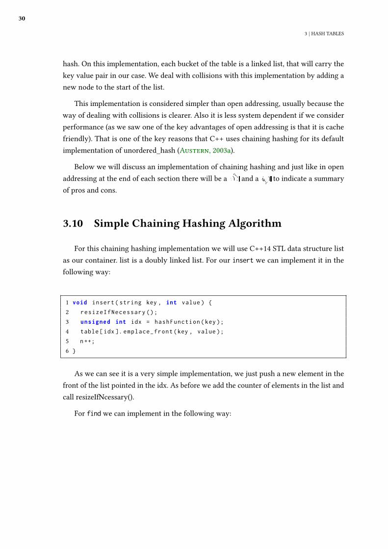
3.10 Simple Chaining Hashing Algorithm

For this chaining hashing implementation we will use C++14 STL data structure listas our container. list is a doubly linked list. For our insert we can implement it in thefollowing way:

1 void insert ( string key , int value ) {

2 r e s i z e I f N e c e s s a r y () ;

3 unsigned int idx = h a s h F u n c t i o n ( key ) ;

4 table [ idx ]. e m p l a c e _ f r o n t ( key , value ) ;

5 n ++;

6 }

As we can see it is a very simple implementation, we just push a new element in thefront of the list pointed in the idx. As before we add the counter of elements in the list andcall resizeIfNcessary().

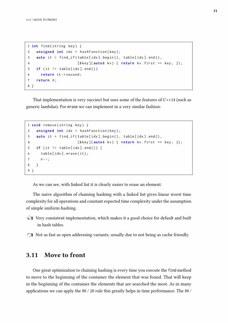
For find we can implement in the following way:

3.11 | MOVE TO FRONT

31

1 int find ( string key ) {

2 unsigned int idx = h a s h F u n c t i o n ( key ) ;

3 auto it = find_if ( table [ idx ]. begin () , table [ idx ]. end () ,

4 [& key ]( auto & kv ) { return kv . first == key ; }) ;

5 if ( it != table [ idx ]. end () )

6 return it - > second ;

7 return 0 ;

8 }

That implementation is very succinct but uses some of the features of C++14 (such asgeneric lambdas). For erase we can implement in a very similar fashion:

1 void remove ( string key ) {

2 unsigned int idx = h a s h F u n c t i o n ( key ) ;

3 auto it = find_if ( table [ idx ]. begin () , table [ idx ]. end () ,

4 [& key ]( auto & kv ) { return kv . first == key ; }) ;

5 if ( it != table [ idx ]. end () ) {

6 table [ idx ]. erase ( it ) ;

7 n - -;

8 }

9 }

As we can see, with linked list it is clearly easier to erase an element.

The naive algorithm of chaining hashing with a linked list gives linear worst timecomplexity for all operations and constant expected time complexity under the assumptionof simple uniform hashing.

u Very consistent implementation, which makes it a good choice for default and builtin hash tables.

d Not as fast as open addressing variants, usually due to not being as cache friendly.

3.11 Move to front

One great optimization to chaining hashing is every time you execute the find methodto move to the beginning of the container the element that was found. That will keepin the beginning of the container the elements that are searched the most. As in manyapplications we can apply the 80 / 20 rule this greatly helps in time performance. The 80 /

32

3 | HASH TABLES

20 rule is basically the idea that usually, 20% of the keys will represent 80% of the searches,this rule is also cited by Knuth (Knuth, 1973).

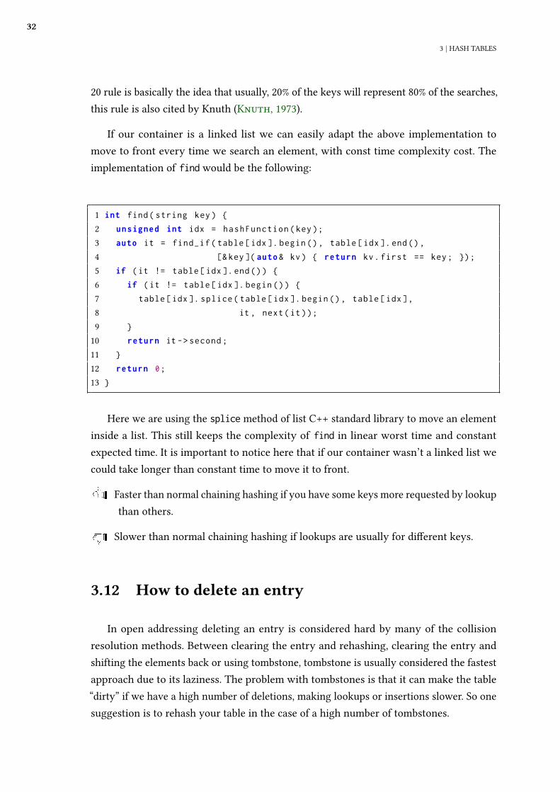
If our container is a linked list we can easily adapt the above implementation tomove to front every time we search an element, with const time complexity cost. Theimplementation of find would be the following:

1 int find ( string key ) {

2 unsigned int idx = h a s h F u n c t i o n ( key ) ;

3 auto it = find_if ( table [ idx ]. begin () , table [ idx ]. end () ,

4 [& key ]( auto & kv ) { return kv . first == key ; }) ;

5 if ( it != table [ idx ]. end () ) {

6 if ( it != table [ idx ]. begin () ) {

7 table [ idx ]. splice ( table [ idx ]. begin () , table [ idx ] ,

8 it , next ( it ) ) ;

9 }

10 return it - > second ;

11 }

12 return 0 ;

13 }

Here we are using the splice method of list C++ standard library to move an elementinside a list. This still keeps the complexity of find in linear worst time and constantexpected time. It is important to notice here that if our container wasn’t a linked list wecould take longer than constant time to move it to front.

u Faster than normal chaining hashing if you have some keys more requested by lookupthan others.

d Slower than normal chaining hashing if lookups are usually for di�erent keys.

3.12 How to delete an entry

In open addressing deleting an entry is considered hard by many of the collisionresolution methods. Between clearing the entry and rehashing, clearing the entry andshifting the elements back or using tombstone, tombstone is usually considered the fastestapproach due to its laziness. The problem with tombstones is that it can make the table“dirty” if we have a high number of deletions, making lookups or insertions slower. So onesuggestion is to rehash your table in the case of a high number of tombstones.

3.13 | WHEN TO RESIZE AN ARRAY

33

In contrast, deleting an entry in chaining hashing is delegated to the container thatcontains the key. That is, if we have a linked list as our container we just delegate thedeletion to it. This is much easier is create less problems than open addressing deletion.That is one of the reasons why chaining hashing is usually chosen for default hash tableimplementation in many languages, like in C++ (Austern, 2003b).

3.13 When to resize an array

In open addressing the load factor to resize a hash table can’t be greater than 1.0,because the table can’t have more elements than its capacity. That is not true for chaininghashing as we will see later on. A good load factor depends on several factors, such as thestrategy used. Some strategies are more “permissive” of a load factor closer to 1, RobinHood for example can still work well with load factors close to 0.9 and doesn’t lose muchperformance with load factors greater than that (Sylvan, 2013). On the other hand, CuckooHashing doesn’t work well with load factors greater than 0.5. Higher load factors meansa better use o memory, which is an advantage of Open Addressing, where lower loadfactors means more memory used but greater e�ciency when using the data structure.For that reason we try to always use the greater load factor possible without degradingmuch performance when using open addressing. In general this value ranges from 0.3 forcuckoo hashing up to .9 for Robin Hood hashing.

In contrast to open addressing, chaining hashing can have max load factors greaterthan 1.0, although many times those are not used, and when they are used they are notfar from 1.0. Default hash tables of C++ and Java use chaining hashing, and the max loadfactor for a hash table in C++ is 1.0, while for java is 0.75. (C++, 2019). It can be easilyproven that the expected time complexity for operations in chaining hashing is O(1 + �)where � is the max load factor. For that reason an big alphas still works reasonably wellwith chaining hashing. Golang for example has 6.5 as max load factor. Although chaininghashing can still work well with bigger load factors it ends up using more memory andalso has a worse locality for cache purposes.

3.14 Open Addressing vs Chaining Hashing

When comparing Open Addressing vs Chaining hashing we can cite many pros andcons. Let us start with the open addressing pros. Among the pros of open addressing wecan see that open addressing techniques such as linear probing tend to be more cache

34

3 | HASH TABLES

friendly. That is because as the key value pairs are stored in the memory in a sequentialway with the vector, when loading a key value pair we will load a chunck of memory thatis around it (that will have other key value pairs). Related to it is the 80 / 20 rule, that whenapplied to hash tables means that “in practice” 80% of the keys will be accessed 20% of thetime (and 20% of the keys will be accessed 80% of the time). This is only for illustrationpurposes, obviously this is not valid for every application, as we can arti�cially createone that does not follow the rule. Another advantage of open addressing is that all thememory will be in a single and sequential “Block” of memory.

35

Chapter 4

Applications

Hash functions and hash tables have a great number of applications in computerscience. In this chapter we present applications of hash functions in algorithms, and otherareas (like cryptography, data deduplication and caching).

We focus in two applications: Rabin-Karp (Wikipedia, 2019e) string matching algorithmand hashing of a rooted tree for isomorphism checking. Rabin-karp string matchingalgorithm is one of the main application of a technique called rolling hashing. Hashingof rooted tree for isomorphism checking (rng_58, 2017) is an interesting applicationsometimes used in competitive programming.

We start by presenting the so called 3-sum problem as a motivation.

4.1 3-sum problem

The problem is stated as following:

“Make a function that given an array of integer numbers and an integer S, it returnsif there are any 3 di�erent elements in this array that its sum equals S. Assume that thereare no three di�erent elements in the array that over�ow a 32-bit integer when summedtogether.”

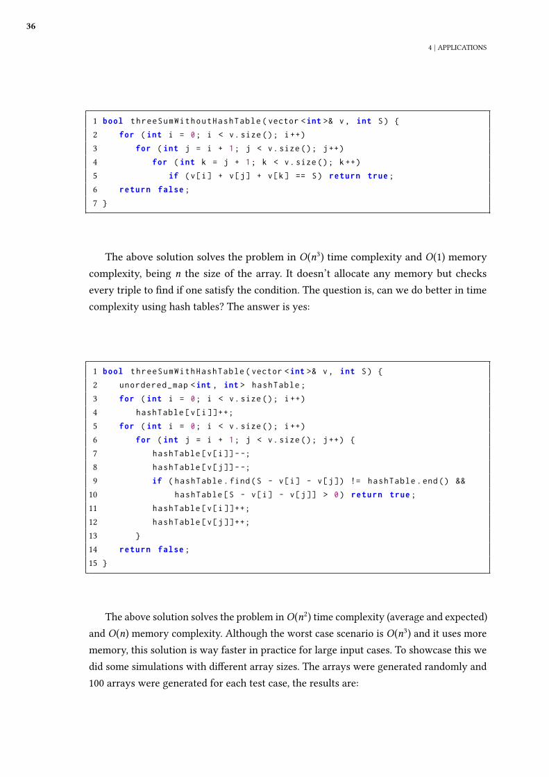
This a very interesting problem that has many di�erent solutions. To start we presentthe brute force solution:

36

4 | APPLICATIONS

1 bool t h r e e S u m W i t h o u t H a s h T a b l e ( vector < int >& v , int S ) {

2 for ( int i = 0 ; i < v . size () ; i ++)

3 for ( int j = i + 1 ; j < v . size () ; j ++)

4 for ( int k = j + 1 ; k < v . size () ; k ++)

5 if ( v [ i ] + v [ j ] + v [ k ] == S ) return true ;

6 return false ;

7 }

The above solution solves the problem in O(n3) time complexity and O(1) memory

complexity, being n the size of the array. It doesn’t allocate any memory but checksevery triple to �nd if one satisfy the condition. The question is, can we do better in timecomplexity using hash tables? The answer is yes:

1 bool t h r e e S u m W i t h H a s h T a b l e ( vector < int >& v , int S ) {

2 unordered_map < int , int > hashTable ;

3 for ( int i = 0 ; i < v . size () ; i ++)

4 hashTable [ v [ i ]]++;

5 for ( int i = 0 ; i < v . size () ; i ++)

6 for ( int j = i + 1 ; j < v . size () ; j ++) {

7 hashTable [ v [ i ]] - -;

8 hashTable [ v [ j ]] - -;

9 if ( hashTable . find ( S - v [ i ] - v [ j ]) != hashTable . end () &&

10 hashTable [ S - v [ i ] - v [ j ]] > 0 ) return true ;

11 hashTable [ v [ i ]]++;

12 hashTable [ v [ j ]]++;

13 }

14 return false ;

15 }

The above solution solves the problem in O(n2) time complexity (average and expected)and O(n) memory complexity. Although the worst case scenario is O(n3) and it uses morememory, this solution is way faster in practice for large input cases. To showcase this wedid some simulations with di�erent array sizes. The arrays were generated randomly and100 arrays were generated for each test case, the results are:

4.2 | RABIN-KARP

37

ArraySize Time Without Hash Table Time with Hash Table Increase in Performance128 4.231ms 6.494ms -53.4%256 34.223ms 26.665ms 22.0%512 267.499ms 99.130ms 62.9%1024 1742.688ms 302.453ms 82.6%2048 7345.126ms 683.197ms 90.6%4096 25029.888ms 761.363ms 96.9%

As we can see in the table above, the three sum solution using hash table quicklysurpasses the brute force implementation. To learn more about how the tests were made,you can check the GithubRepo (Moura, 2019).

4.2 Rabin-Karp

Rabin Karp is a famous pattern matching on string algorithm. Di�erently than otherclassic solutions to pattern matching, such as Knuth-Morris-Pratt (Wikipedia, 2019d)algorithm or Boyer Moore (Wikipedia, 2019a), Rabin Karp is based on hashing. It relieson the property that if the hashes of two strings are not equal, they are certainly di�erentstrings, and if they are equal, they can be the same string. The de�nition of the patternmatching problem is the following:

“Make a function that given two strings, one string t and one string p, it returns the indexof the �rst occurrence of p in t, or -1 if p is not present in t. It is guaranteed that the length oft is greater than the length of p.”

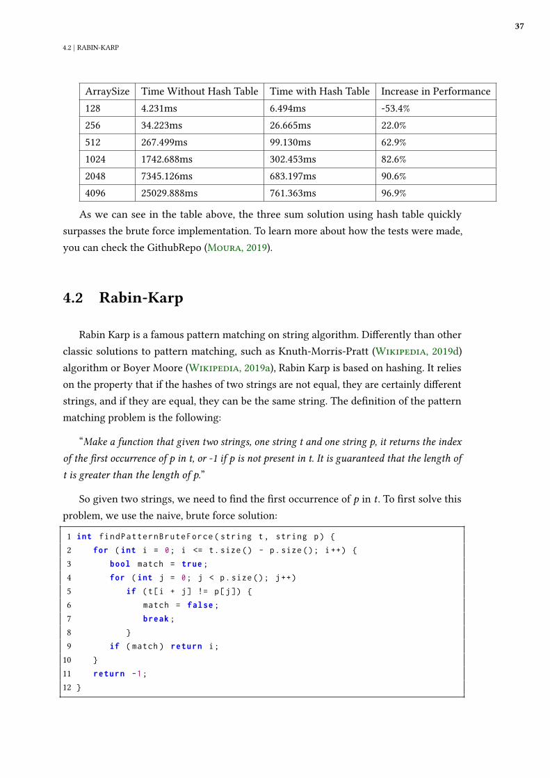
So given two strings, we need to �nd the �rst occurrence of p in t . To �rst solve thisproblem, we use the naive, brute force solution:

1 int f i n d P a t t e r n B r u t e F o r c e ( string t , string p ) {

2 for ( int i = 0 ; i <= t . size () - p . size () ; i ++) {

3 bool match = true ;

4 for ( int j = 0 ; j < p . size () ; j ++)

5 if ( t [ i + j ] != p [ j ]) {

6 match = false ;

7 break ;

8 }

9 if ( match ) return i ;

10 }

11 return -1 ;

12 }

38

4 | APPLICATIONS

We can see that the brute force solution has worst case scenario of O(nm) being n = |t |,the size of the string t , and m = |p|, the size of the string p. One possible optimization forthis solution is if we could check a text interval against the pattern quicker than O(m). Ifwe had the hash of the pattern and the hash of the text interval, we could easily do that. Thehash of the pattern is constant, but we have O(n) intervals to check, and given that eachinterval has O(m) size, if we calculated each of them alone this would take O(nm) again.However, for some hash functions, given the hash of an interval we could calculate thenext hash faster. One example of a hash function with this property is the dumbHasℎXORhash function presented in chapter 1. Lets test it with intervals in “abracadabra” withintervals of size 4:

dumbHasℎXOR(′brac′) = dumbHasℎXOR(′abra′) ⊕ ′a′ ⊕ ′c′

So given the hash of ’abra’ we could easily move to ’brac’. Functions with this“shifting” property are called rolling hash functions. As we saw in the hash functionchapter, “dumbHashXOR” is, generally, a not so good hash function. Hopefully, we havebetter rolling hash functions for that, one example is polynomial hashing. The polynomialhashing of a string s with prime P would be:

m−1

∑

i=0

s[i] × Pi

So we know that given hash of s[0 . . m−1] we can calculate the hash of s[1 . . m] inO(1) in the following way:

PolynomialHasℎ(s[1 . . m]) =

m

∑

i=1

s[i] × Pi−1=

m−1

∑

i=0

s[i] × Pi− s[0] + s[m] × P

m−1

We would just need to store Pm−1 for recalculating the hash. So we can check if thepattern is matched on the text quicker with hashing. As just hashing may return a matchwhere we don’t have a match, we need to double check to have 100% accuracy. So thealgorithm will be:

4.2 | RABIN-KARP

39

1 const int PRIME = 3 3 ;

2 const int MOD = 1 0 0 0 0 3 3 ;

3 int f i n d P a t t e r n R a b i n K a r p ( string t , string p ) {

4 int textHash = 0 , p a t t e r n H a s h = 0 ;

5 int pot = 1 ;

6 // pot will be PRIME ^{ p . size () - 1}

7 for ( int i = 0 ; i < p . size () - 1 ; i ++)

8 pot = ( pot * PRIME ) % MOD ;

9 for ( int i = 0 ; i < p . size () ; i ++) {

10 textHash = ( textHash * PRIME + t [ i ]) % MOD ;

11 p a t t e r n H a s h = ( p a t t e r n H a s h * PRIME + p [ i ]) % MOD ;

12 }

13 for ( int i = 0 ; i <= t . size () - p . size () ; i ++) {

14 if ( textHash == p a t t e r n H a s h ) {

15 bool match = true ;

16 for ( int j = 0 ; j < p . size () ; j ++)

17 if ( t [ i + j ] != p [ j ]) {

18 match = false ;

19 break ;

20 }

21 if ( match ) return i ;

22 }

23 textHash = ( PRIME * ( textHash - pot * t [ i ]) + t [ i + p . size () ])

% MOD ;

24 if ( textHash < 0 ) textHash += MOD ;

25 }

26 return -1 ;

27 }

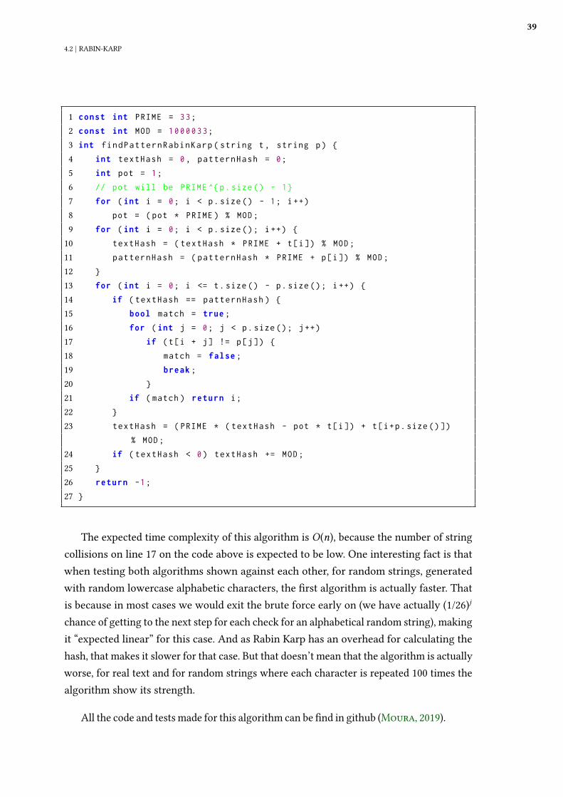
The expected time complexity of this algorithm is O(n), because the number of stringcollisions on line 17 on the code above is expected to be low. One interesting fact is thatwhen testing both algorithms shown against each other, for random strings, generatedwith random lowercase alphabetic characters, the �rst algorithm is actually faster. Thatis because in most cases we would exit the brute force early on (we have actually (1/26)j

chance of getting to the next step for each check for an alphabetical random string), makingit “expected linear” for this case. And as Rabin Karp has an overhead for calculating thehash, that makes it slower for that case. But that doesn’t mean that the algorithm is actuallyworse, for real text and for random strings where each character is repeated 100 times thealgorithm show its strength.

All the code and tests made for this algorithm can be �nd in github (Moura, 2019).

40

4 | APPLICATIONS

4.3 Complete tripartite graph

We can also use hashing for graph problems. This is a pretty speci�c problem but witha very interesting application from the hashing point of view. The problem statement goesas following:

“Given an undirected graph, decide if the vertices can be partitioned in three groups, suchthat no two vertices of the same group are connected and every two vertices of di�erent groupsare connected .”

That is, given a graph decide if the graph is a tripartite complete graph.

We can notice that all the vertices from a partition will have the same adjacency list(They will be adjacent all the other vertices). From that we can hash every adjacency listinto an integer, and divide the nodes in groups. If we have 3 groups, we have a potentialtripartition. Then we can double check if all the vertices in a partition have an adjacency listof size n−partitionSize, where n is the number of vertices in the graph and partitionSizeis the size of the partition. That will guarantee that they are pointing to all vertices outsidethe partition.

For the hashing algorithm in the solution of this problem, we can use any of the hashingalgorithms described in the �rst chapter, as we can see an array of integers as a string. Ifwe use a hashing algorithm that is not dumbXOR or dumbADD, we need to �rst sort thearray to ensure that all equivalent lists will have the same array.

If we use dumbXOR or dumbADD, one thing that can help to minimize collisions isto give each vertex a random value in a greater set. For example if we have n = 105 for thesize of our graph, we can map the nodes to a random value between 0 and 109 + 7. Thatwould increase the size of our potential hashes, minimizing the possible collisions. Thisproblem can be seen in codeforces: h�ps://codeforces.com/contest/1228/problem/D

4.4 Hashing trees to check for isomorphism

For this last algorithmic application of hash functions and hash tables we describehow to decide if two rooted trees are isomorphic. We say that two trees, T1 and T2 areisomorphic if there is a bijection � between the set of vertices V1 and V2 of the trees, suchthat:

4.4 | HASHING TREES TO CHECK FOR ISOMORPHISM

41

∀u, v ∈ V1 u adjT1v ⟺ �(u) adjT2

�(v)

That is, if u is adjacent to v in the �rst tree, �(u) must be adjacent to �(v) in the secondtree and vice-versa.

Given that de�nition, we can state the problem of deciding if two trees are isomor-phic:

“Write a function that given two rooted trees, decide if they are isomorphic.”

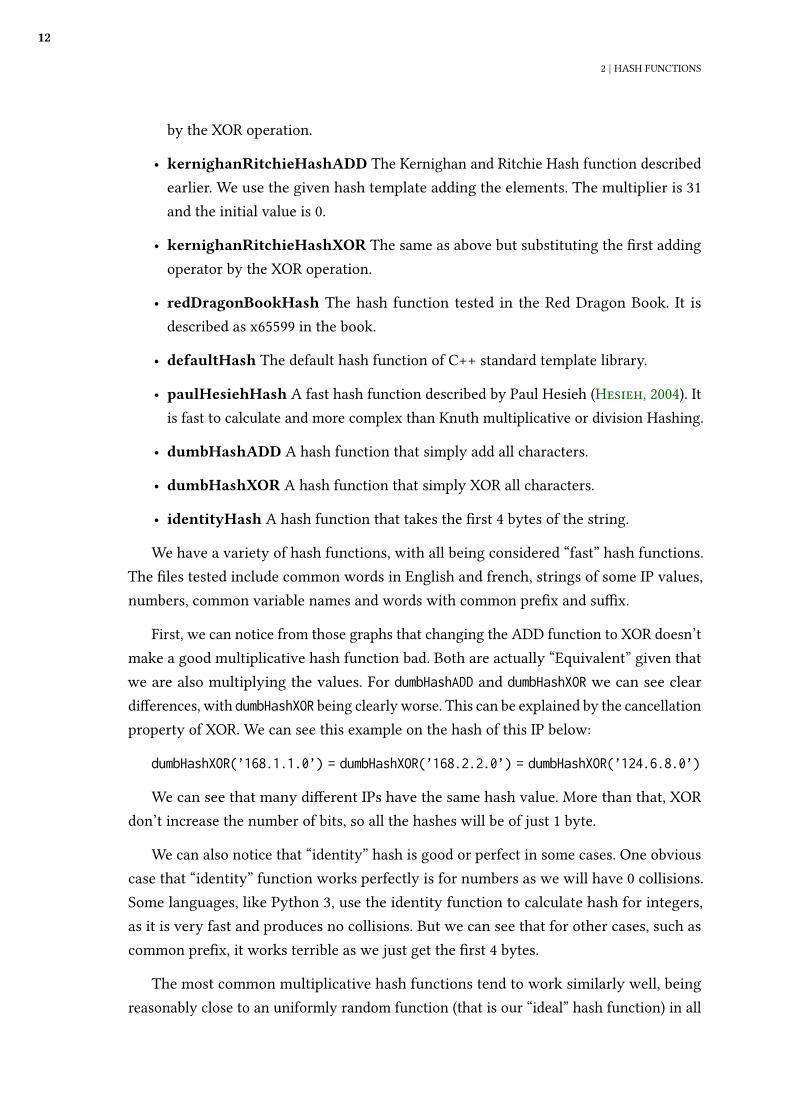
We could solve this problem using hash functions if we knew how to hash trees tointegers. As we saw in the �rst chapter, everything is bits in the end and we just need asmart way of representing our data. We can represent a rooted tree as a node that pointsto its child nodes and so on. So we could de�ne a hash function that always collide whenwe have isomorphic trees. The following hash function was described by competitiveprogrammer rng_58 in his blog (rng_58, 2017).

Hasℎ(N ) =

⎧⎪⎪

⎨⎪⎪⎩

x0 if N is a leaf (has no childs)

Πk

i=1(xd + Hasℎ(Ci)) modM where Ci is a child node, and d is the height of N

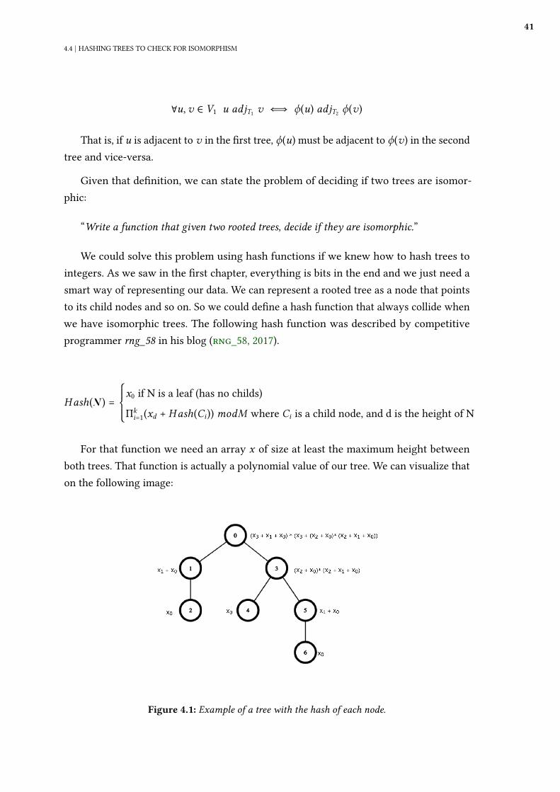
For that function we need an array x of size at least the maximum height betweenboth trees. That function is actually a polynomial value of our tree. We can visualize thaton the following image:

Figure 4.1: Example of a tree with the hash of each node.

42

4 | APPLICATIONS

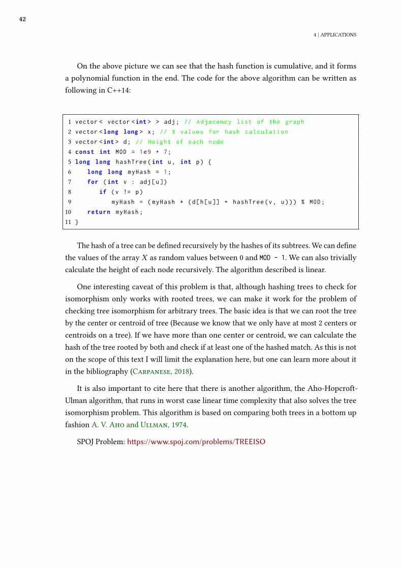
On the above picture we can see that the hash function is cumulative, and it formsa polynomial function in the end. The code for the above algorithm can be written asfollowing in C++14:

1 vector < vector < int > > adj ; // Adjacency list of the graph

2 vector < long long > x ; // X values for hash c a l c u l a t i o n

3 vector < int > d ; // Height of each node

4 const int MOD = 1 e 9 + 7 ;

5 long long hashTree ( int u , int p ) {

6 long long myHash = 1 ;

7 for ( int v : adj [ u ])

8 if ( v != p )

9 myHash = ( myHash * ( d [ h [ u ]] + hashTree (v , u ) ) ) % MOD ;

10 return myHash ;

11 }

The hash of a tree can be de�ned recursively by the hashes of its subtrees. We can de�nethe values of the array X as random values between 0 and MOD - 1. We can also triviallycalculate the height of each node recursively. The algorithm described is linear.

One interesting caveat of this problem is that, although hashing trees to check forisomorphism only works with rooted trees, we can make it work for the problem ofchecking tree isomorphism for arbitrary trees. The basic idea is that we can root the treeby the center or centroid of tree (Because we know that we only have at most 2 centers orcentroids on a tree). If we have more than one center or centroid, we can calculate thehash of the tree rooted by both and check if at least one of the hashed match. As this is noton the scope of this text I will limit the explanation here, but one can learn more about itin the bibliography (Carpanese, 2018).

It is also important to cite here that there is another algorithm, the Aho-Hopcroft-Ulman algorithm, that runs in worst case linear time complexity that also solves the treeisomorphism problem. This algorithm is based on comparing both trees in a bottom upfashion A. V. Aho and Ullman, 1974.

SPOJ Problem: h�ps://www.spoj.com/problems/TREEISO

43

Chapter 5

Final Remarks

As we can see by previous chapters, hash functions and hash tables are very widetopics, with several details that we can have pages and pages with explanations. This textaimed to provide a glance on how to implement a hash table data structure, with someother applications of the hash function itself.

It is important to notice that almost every programming language has it’s implemen-tation of a hash table, with some having a built-in implementation of a hash functionfor external usage. The most famous that we can cite here is Java, C++ (which havean implementation on STL), Golang, Python, Ruby, C# and Scala. Its implementationmay di�er among paradigms as well, for example although in Scala Mutable hash mapsuses chaining hashing, it also uses a Hash Trie for immutable hash maps, which is acomplete di�erent implementation with it’s own speci�calities and bene�ts for functionalprogramming languages. (Cohen, 2017)

Another interesting fact about hash tables is that it is an example about how memorylocality is important in modern data structures. Memory locality is the proximity of thedata accessed, which means that the data of your data structure is close to each otherand it is “cache friendly”. Although not accounted by usual complexity analysis, it is animportant factor for regular used data structures, as one of the key performance factors ofmodern day processors.

During this text I also realized how deep we can go in each hash related topic. Forthat reason there are many contents that are not included here but are interesting to learnabout. The main topics that would be included if I had more time were:

• Consistent Hashing

• Distributed Hash Table

44

5 | FINAL REMARKS

• A deep analysis of the hash tables implemented during this text

Consistent hashing is a very interesting topic, because it is a special kind of hashfunction commonly used to implement sharded databases. It is special because when thetable is resized, only K

nkeys need to be remapped on average, where K is the number of

keys and N is the number of slots.(Wikipedia, 2019b) This is very interesting and veryuseful in the context of databases because it easily allows horizontal scaling (that is, addingmore machines).

Another interesting topic that I would have liked to discuss is distributed hash tables.A very used application in modern day, distributed hash table is a service that simulateda hash table lookup in a distributed environment. Common examples of this is modernservices such as Memcached and Redis, that allow fast responses and scaling in modernweb applications.

Lastly, it would be interesting to do a deep analysis of the hash tables implementedduring this text. This would be di�erent because we would see in practice many of thetrade-o�s discussed during this text, such as memory locality. There are many di�erentfactors in a deep analysis like this, like testing with di�erent load factors, di�erent deletingstrategies, and di�erent queries (random queries or queries closer to the 80/20 rule).

45

References

[Aho et al. 1986] Alfred V. Aho, Monica S. Lam, Ravi Sethi, and Je�rey D. Ullman.Compilers: Principles, Techniques, and Tools. Pearson Education, Inc, 1986 (cit. onpp. 5, 9).

[A. V. Aho and Ullman 1974] J. E. Hopcroft A. V. Aho and J. D. Ullman. “The Designand Analysis of Computer Algorithms”. In: Addison-Wesley (1974) (cit. on p. 42).

[Austern 2003a] Matthew Austern. A Proposal to Add Hash Tables to the StandardLibrary (revision 4). 2003. url: h�p://www.open-std.org/jtc1/sc22/wg21/docs/

papers/2003/n1456.html (cit. on p. 30).

[Austern 2003b] Matthew Austern. A Proposal to Add Hash Tables to the StandardLibrary (revision 4). 2003. url: h�p://www.open-std.org/jtc1/sc22/wg21/docs/

papers/2003/n1456.html (cit. on p. 33).

[Bernstein 1991] Bernstein. djb2. 1991. url: h�p://www.cse.yorku.ca/~oz/hash.html

(cit. on p. 9).

[C++ 2019] C++. C++ Reference max_load_factor. 2019. url: h�p://www.cplusplus.com/

reference/unordered_set/unordered_set/max_load_factor/ (cit. on p. 33).

[Carpanese 2018] Igor Carpanese. An illustrated introduction to centroid decomposition.2018. url: h�ps : / /medium.com/carpanese/an- illustrated- introduction- to-

centroid-decomposition-8c1989d53308 (cit. on p. 42).

[Celis 1986] Pedro Celis. “Robin Hood Hashing”. In: Waterloo PhD Research (1986).url: h�ps://cs.uwaterloo.ca/research/tr/1986/CS-86-14.pdf (cit. on pp. 6, 22, 23).

[Cohen 2017] Russel Cohen. An Analysis of Hash Map Implementations in PopularLanguages. 2017. url: h�ps://rcoh.me/posts/hash-map-analysis/ (cit. on p. 43).

46

REFERENCES

[Facebook 2019] Facebook. “F14 is Open Sourced”. In: Facebook Blog (2019). url: h�ps:

//engineering.fb.com/developer-tools/f14/ (cit. on p. 3).

[Hesieh 2004] Paul Hesieh. Hash functions. 2004. url: h�p://www.azillionmonkeys.

com/qed/hash.html (cit. on p. 12).

[Kankowski 2008] Peter Kankowski. Hash functions: An empirical comparison. 2008.url: h�ps://www.strchr.com/hash_functions (cit. on pp. 8, 10, 11).

[Knuth 1973] Donald Knuth. The Art of Computer Programming, Volume 3: Sortingand Searching. Addison-Wesley, 1973 (cit. on pp. i, iii, 2, 6, 7, 27, 32).

[Kernighan and Ritchie 1988] Brian W Kernighan and Dennis M. Ritchie. The Cprogramming language, second edition. Prentice Hall Software Series, 1988 (cit. onp. 9).

[Moura 2019] Breno Helfstein Moura. Code for Undergraduate thesis. 2019. url: h�ps:

//github.com/breno-helf/TCC/tree/master/monografia/code (cit. on pp. 11, 37,39).

[rng_58 2017] rng_58. Hashing and Probability of Collision. 2017. url: h�p : / / rng-

58.blogspot.com/2017/02/hashing-and-probability-of-collision.html (cit. onpp. 35, 41).

[Sylvan 2013] Sebastian Sylvan. Robin Hood Hashing should be your default Hash Tableimplementation. 2013. url: h�ps://www.sebastiansylvan.com/post/robin-hood-

hashing-should-be-your-default-hash-table-implementation/ (cit. on p. 33).

[Wikipedia 2019a] Wikipedia. Boyer-Moore string-search Algorithm. 2019. url: h�ps:

//en.wikipedia.org/wiki/Boyer-Moore_string-search_algorithm (cit. on p. 37).

[Wikipedia 2019b] Wikipedia. Consistent Hashing. 2019. url: h�ps://en.wikipedia.org/

wiki/Consistent_hashing (cit. on p. 44).

[Wikipedia 2019c] Wikipedia. Hash Function. 2019. url: h�ps://en.wikipedia.org/wiki/

Hash_function (cit. on p. 5).

[Wikipedia 2019d] Wikipedia. Knuth-Morris-Pratt Algorithm. 2019. url: h�ps://en.

wikipedia.org/wiki/Knuth-Morris-Pra�_algorithm (cit. on p. 37).

REFERENCES

47

[Wikipedia 2019e] Wikipedia. Rabin Karp. 2019. url: h�ps://en.wikipedia.org/wiki/

Rabin-Karp_algorithm (cit. on p. 35).