EVALUATION OF NANOFILTRATION FOR THE TREATMENT … Hub Documents/Research Reports/1230-… ·...
137
EVALUATION OF NANOFILTRATION FOR THE TREATMENT OF RURAL GROUNDWATER FOR POTABLE WATER USE Report to the WATER RESEARCH COMMISSION by S J Modise 1 and H M Krieg 2 Durban Institute of Technology 1 Vaal University of Technology 2 North-West University WRC Report No 1230/1/04 ISBN No 1-77005-150-3 MARCH 2004
Transcript of EVALUATION OF NANOFILTRATION FOR THE TREATMENT … Hub Documents/Research Reports/1230-… ·...
EVALUATION OF NANOFILTRATION FOR THE
TREATMENT OF RURAL GROUNDWATER FOR
POTABLE WATER USE
Report to the WATER RESEARCH COMMISSION
by
S J Modise1and H M Krieg2 Durban Institute of Technology
1Vaal University of Technology
2North-West University
WRC Report No 1230/1/04 ISBN No 1-77005-150-3
MARCH 2004

Disclaimer This report emanates from a project financed by the Water Research Commission (WRC) and is approved for publication. Approval does not signify that the contents necessarily reflect the views and policies of the WRC or the members of the project steering committee, nor does mention of trade names or commercial products constitute endorsement or recommendation for use.

ii
Contents
Contents ii
List of Tables iv
List of Figures v
Executive Summary viii
Acknowledgments xii
1 Background 1
1.1 Introduction 1
1.2 Motivation 1
2 Literature review 3
2.1 Nanofiltration – Historical background 3
2.2 Development of membranes in South Africa 4
2.3 Membrane processes 6
2.4 Pressure driven processes 6
2.5 Fouling 7
2.6 Summary and conclusion 10
3 Dead-end NF and preliminary tests 17
3.1 Filtration set-up 17
3.2 Membranes 18
3.3 Permeation measurements 19
3.4 Nanofiltration of salts 22
3.5 Theory 23
3.6 Tests 23
3.7 Summary and conclusion 37
4 Building and testing the cross-flow unit 40
4.1 Capacity 40
4.2 Avoiding rusting of equipment 42
4.3 Possibility of transporting the unit 42
iii
4.4 Operation modes and parameters 43
4.5 Process Flow Diagram 44
4.6 Testing the unit 47
5 Treatment of rural water 51
5.1 Pollution and its effect 51
5.2 Experimental 52
5.3 Water classification methodology 54
5.4 Water sampling and monitoring 57
5.5 Water classification results 60
5.6 Water treatment 62
5.7 Dead-end studies 63
5.8 Cross-flow studies 72
5.9 Summary and Conclusion 76
6 Evaluation and recommendations 80
6.1 Evaluation 80
6.2 Highlights 81
6.3 General discussions 82
6.4 Recommendations and further research 83

iv
Appendix A 84
Appendix B 86
Appendix C 87
Appendix D 88
Appendix E 89
Appendix F 90
Appendix G 93
Appendix H 97
Appendix I 98
Appendix J 99
Appendix K 107
Appendix L 110
Appendix M 113
Appendix N 114
Appendix O 115
Appendix P 117
Appendix Q 119
Appendix R 121
Appendix S 123
List of Tables
Table 3. 1 Specifications of NF-membranes 18
Table 3. 2 Clean water permeability and porosity value of NF-membranes 22
Table 3. 3 Single salt retentions of (2-1), (1-1), and (1-2) salts on different membranes 28
Table 4.1 Pressure drop over the system as a function of the pipe diameter used 42

v
Table 5. 1 List of locations where water samples were collected 53
Table 5. 2 Colour code classification and effects of components in water intended for domestic use 55
Table 5. 3 Concentration ranges of various chemical components used in water colour classification 56
Table 5. 4 The Rustenburg region water classification for maximum concentration values observed 60
Table 5. 5 The Rustenburg region water classification for average concentration values observed 61
Table 5. 6 Initial concentration (feed), permeate and brine of sampled and treated water by NF membranes on a dead-end mode unit. 71
Table 5. 7 Sampled water chemical composition and characteristics 72
Table 5. 8 Water classification (fluoride) before and after treatment by various nanofiltration membranes 78
List of Figures
Figure 2. 1 Dead-end (A) and cross-flow (B) membrane processes 7
Figure 2. 2 The concentration polarization phenomenon 8
Figure 2. 3 Pore blocking mechanisms (A: complete pore blocking, entrance to pore sealed, B: pore bridging: partial obstruction to entrance, C: internal pore binding, entrapment/adsorption of non-retained species), D: lateral cake formation 9
Figure 3. 1 The high-pressure dead-end module 17
Figure 3. 2 Water flux- time plot on TFC-S nanofiltration membrane (T = 25oC, cross flow module) 21
Figure 3. 3 Water flux – pressure plot for different membranes (T = 25oC, dead-end module) 21
Figure 3. 4 Solute flux – pressure relations of varying NaCl concentrations through different membranes (T = 25oC, dead-end mode) 25
Figure 3. 5 Retention versus concentrations of (2-1), (1-1), and (1-2) salts (anions) 27
vi
Figure 3. 6 Retention – pressure relation showing the effect of stirring on TFC-SR membrane (T = 25oC, dead-end mode) 29
Figure 3. 7 Flux – pressure relations showing the effect of stirring on TFC-SR membrane (50ppm CaSO4, T = 25oC, dead-end mode) 30
Figure 3. 8 Rejection of NaCl and Na2SO4 mixture on 3 different membranes (pressure = 10 bar, total Na+ concentration = 200ppm) 31
Figure 3. 9 Rejection of CaSO4 and CaCl2 mixture on 3 different membranes (pressure = 10 bar, total Ca2+ concentration = 200ppm) 33
Figure 3. 10 Rejection of NaCl and CaCl2 mixtures on 3 different membranes (pressure = 10 bar, total Cl- concentration = 200ppm) 35
Figure 3. 11 Rejections of Na2SO4 and CaSO4 mixtures on 3 different membranes (pressure = 10 bar, total SO4
2- concentration = 200ppm) 36
Figure 3. 12 Rejection of CaCl2and CaF2 mixtures on TFC-SR (pressure = 10 bar, F- concentration = 5ppm) 37
Figure 4. 1 Process flow diagram of sand filter, micro-filter and NF unit in series 44
Figure 4. 2 Process flow diagram of the NF unit 45
Figure 4. 3 Modified NF unit diagram 46
Figure 4. 4 Permeabilities of clean water on various membranes 47
Figure 4. 5 Volume flux and retention coefficient of various salts on various membranes 49
Figure 5. 1 Selected chemical component concentrations recorded for various sampling sites during the wet season (A = Klerksdorp, B = Koster, C = Rustenburg, and D = Mafikeng Regions. X-axis = sampling points) 57
Figure 5. 2 Selected chemical component concentrations recorded for various sampling sites during dry seasons (A = Klerksdorp, B = Koster, C = Rustenburg, and D = Mafikeng Regions. X-axis = sampling points) 58
Figure 5. 3 Average chemical component concentrations recorded for various sampling sites over one year (A = Klerksdorp, B = Koster sub-, C = Rustenburg, and D = Mafikeng Regions. X-axis = sampling points) 59
vii
Figure 5. 4 Retention coefficient of various NF membranes on the treatment of the Lerome groundwater (Pressure = 20 bar, temperature = 20oC. x-axis = membrane types) 64
Figure 5. 5 Presentation of membrane performance for Lerome groundwater (Pressure = 20 bar, temperature = ambient) 65
Figure 5. 6 Retention coefficient of various NF membranes on the treatment of the Ledig rural water (Pressure = 20 bar, temperature = 20oC. x-axis = membrane types) 66
Figure 5. 7 Presentation of membrane performance on Ledig rural water (Pressure = 20 bar, temperature = ambient) 66
Figure 5. 8 Retention coefficient of various NF membranes on the treatment of the Haaskraal water components (Pressure = 20 bar, temperature = 20oC. x-axis = membrane type) 67
Figure 5. 9 Presentation of membrane performance on Haaskraal rural water (Pressure = 20 bar, temperature = ambient) 68
Figure 5. 10 Retention coefficient of various NF membranes on the treatment of Vaal River water (Pressure = 20 bar, temperature = 20oC. x-axis = membrane type) 69
Figure 5. 11 Presentation of the membrane performance on Vaal River water (Pressure = 20 bar, temperature = ambient) 70
Figure 5. 12 Presentation of the membrane performance on Lerome water (Pressure = 5bar, temperature = ambient, cross-flow) 73
Figure 5. 13 Presentation of the membrane performance on Ledig water (Pressure = 5bar, temperature = ambient, cross-flow) 74
Figure 5. 14 Presentation of the membrane performance on Haaskraal water (Pressure = 5bar, temperature = ambient, cross-flow) 74
Figure 5. 15 Presentation of the membrane performance on Vaal River water (Pressure = 5bar, temperature = ambient, cross-flow) 75
viii
EVALUATION OF NANOFILTRATION FOR THE TREATMENT OF
RURAL GROUNDWATER FOR POTABLE WATER USE
EXECUTIVE SUMMARY
Clean drinking water and sanitation, effective wastewater or industrial effluent treatment
and management, and safe and efficient health care facilities and awareness are vital
services to all communities around the world and in particular, South Africa. The South
African government has embarked on the provision of adequate and safe water to all. This
has lead to a more intensive water research than ever before to ensure increasing and
continued supply of drinkable and other survival related water. As a result, a new Water
Services Act evolved to ensure access to water by the many families that never had one
before. Coupled to this Act, is the National Water Act 36 of 1998, which guarantees save
water. The Act guards against pollution and intends to conserve and protect water.
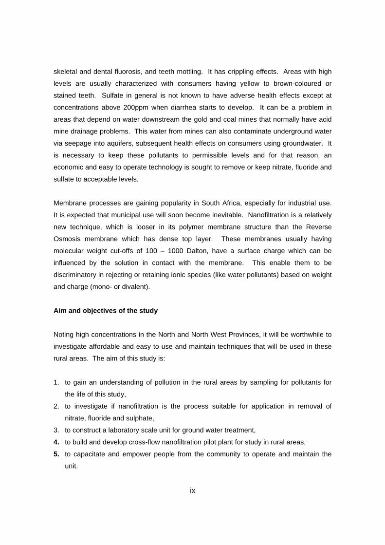
Characterization of rural water
South African rural areas are characterized by underground water abstraction, and largely
depend on this for a living. Apart from this, some areas get their water from streams,
rivers, and springs. Although groundwater is normally “clean”, some areas experience
high levels, than is acceptable, of nitrate, fluoride and in some instances, high sulfate in
their water. Salinity is also of major concern but will however not be dealt with in this
study. These pollutants have their levels higher than the SABS specifications for human
consumption, livestock watering and irrigation. High fluoride concentrations are
experienced in borehole waters in the Mankwe (about 14ppm), Moretele (4 to 5ppm) and
Taung districts (approximately 5ppm). The waters are not fit for human consumption.
Nitrate concentrations are as high as 173ppm in Moretele and 130ppm in Kudumane
districts [1].
High levels of nitrate (>10ppm as N) is known to easily convert the nitrite in the stomach
which in turn get adsorbed in the blood stream. Nitrite hinders or defects oxygen
adsorption and as a result causes oxygen depletion in the blood. Fluoride (>1ppm) causes
ix
skeletal and dental fluorosis, and teeth mottling. It has crippling effects. Areas with high
levels are usually characterized with consumers having yellow to brown-coloured or
stained teeth. Sulfate in general is not known to have adverse health effects except at
concentrations above 200ppm when diarrhea starts to develop. It can be a problem in
areas that depend on water downstream the gold and coal mines that normally have acid
mine drainage problems. This water from mines can also contaminate underground water
via seepage into aquifers, subsequent health effects on consumers using groundwater. It
is necessary to keep these pollutants to permissible levels and for that reason, an
economic and easy to operate technology is sought to remove or keep nitrate, fluoride and
sulfate to acceptable levels.
Membrane processes are gaining popularity in South Africa, especially for industrial use.
It is expected that municipal use will soon become inevitable. Nanofiltration is a relatively
new technique, which is looser in its polymer membrane structure than the Reverse
Osmosis membrane which has dense top layer. These membranes usually having
molecular weight cut-offs of 100 – 1000 Dalton, have a surface charge which can be
influenced by the solution in contact with the membrane. This enable them to be
discriminatory in rejecting or retaining ionic species (like water pollutants) based on weight
and charge (mono- or divalent).
Aim and objectives of the study
Noting high concentrations in the North and North West Provinces, it will be worthwhile to
investigate affordable and easy to use and maintain techniques that will be used in these
rural areas. The aim of this study is:
1. to gain an understanding of pollution in the rural areas by sampling for pollutants for
the life of this study,
2. to investigate if nanofiltration is the process suitable for application in removal of
nitrate, fluoride and sulphate,
3. to construct a laboratory scale unit for ground water treatment,
4. to build and develop cross-flow nanofiltration pilot plant for study in rural areas,
5. to capacitate and empower people from the community to operate and maintain the
unit.

x
During sampling, the areas of the greater Rustenburg region showed high levels of fluoride
and to some extend of nitrate. For the other three regions (Klerksdorp, Mafikeng and
Koster), the levels of these two pollutants were within the limits. The study was continued
on the cross-flow unit using sampled water from selected sites.
Nine commercial NF-membranes (D11, D12, CTC1, NF70, NF90, TFC-S, TFC-SR, TFC-
HR and TFC-ULP) were evaluated in this and another [2] study for their efficiency (flux and
retention) using pure water, non-charged solutes, single and mixed salts as well as
numerous water samples from North West rural areas. All membranes had a negative
surface charge density. While D11, D12 and TFC-SR had the highest flux for all systems
tested, they had the lowest retention in terms of non-charged solutes as well as single
salts. NF70, NF90 and TFC-S displayed reverse osmosis (RO) properties with high
reflection coefficients () but low permeabilities for non-charged solutes and single salts.
Membrane performance varied greatly when using mixed salts (depending on the salt
combinations) and no correlation could be found.
A small laboratory scale NF unit was built to do preliminary studies in terms of screening
and characterising the NF membranes. The NF unit, which could be operated up to 25bar,
was built with the courtesy of Henk Veldhuis (Twente University, Holland).
For rural water treatment and testing of the high-pressure cross-flow NF unit, the best
retention for fluoride and nitrate. All membranes efficiently removed sulfate due to their
negative surface charge. While it was not possible to correlate membrane performance for
different sample sites, TFC-S, TFC-SR, NF70 and NF90 had the best retentions on a
dead-end module, and are recommended for further investigations.
The built high-pressure cross-flow unit was tested for performance by rejecting prepared
solutions of sulfate, nitrate and fluoride. The results were comparable to those of the dead-
end mode studies. In treating rural water, the membrane performance varied slightly from
those observed during dead-end studies. Although the divalent ion (e.g.sulfate) levels
were reduced greatly, monovalent ions were poorly rejected by all membranes, including
the NF70 which showed promising results during the dead-end mode studies.

xi
The backlog of the study was the failure to train and empower community people to
operate the unit. This was because it was difficult to transport the unit to various sites of
interest. The sampled water was instead brought on-site to where the unit was built. The
ease of operation of the unit is recommended for further study.

xii
Acknowledgments
The authors are grateful to the Water Research Commission (WRC) for its financial
support without which this research would not have been possible.
The research focus area Separation Science and Technology (SST) of the
Potchefstroom University for CHE is acknowledged for its fiscal and infrastructure
support.
The help of Hennie van Zyl and Jan Kroeze with the design, manufacture and
commissioning of the pilot plant. The contribution of Japie Scholtz (Sasol
SASTECH) is also acknowledged,
We would like to thank Hein Neomagus for his valuable contributions in terms of
various chemical engineering aspects of the project.
Finally an acknowledgment to Klaas Keizer who fundamentally contributed to the
membrane related education of both authors.
1. Schoeman, J.J., Steyn, A. (2000). Defluoridation, denitrification and desalination of
water using ion-exchange and reverse osmosis technology, Water Research
Commission TT124/00, WRC, Pretoria.
2. Modise, S.J. (2002) South African rural water, Ph.D. Thesis, Potchefstroom
Universityfor CHE, Potchefstroom, South Africa.

1
1 Background
1.1 Introduction
Prosperity of man is, among others, highly dependent on the availability and adequate
supply of clean water. In the past, clean water supply meant clear water. If one water
supply failed then another one would be easily found, as the population was small and
as such water was abundantly available. The principle of the “best available source”
was applied. Water-borne diseases infected some communities over time, and there
had to be a way to treat water prior to drinking. Over the years man became capable
of making water safe from the infectious diseases by the introduction of filtration and
chlorination with subsequent development of water treatment strategies. This resulted
in a shift from using the best available water to using the most economic source [1]. One
of the latest strategies includes the development of membrane processes that will
supplement if not substitute conventional water treatment processes. These
developments result from the ever-growing need for and scarcity of water due to
industrialization and the population increase, which necessitates revision and
development of water regulation.
1.2 Motivation
The development of South Africa in technology advances in terms of industrial,
economic, and international relations requires more cautious environmental
considerations. These include air, water and soil pollution, which singly and collectively
directly affect our health, wealth and prosperity. Added to industrialization are political,
social, economic and demographic changes this country is experiencing. Needless to
say, a decrease in water quality cannot be ignored any longer.
A major water related problem in South Africa (and probably in other countries) is that
of high levels of ionic pollutants in rural water. Here, many people depend on
boreholes as their source of water. Water from some of these boreholes is of low
quality (high levels of nitrate, sulfate, fluoride, salinity, hardness and turbidity). It is not
clear yet as to the underground geohydrological patterns and if these would be the
cause of such pollutants. It is believed however, that degraded water quality is due to
farming practices, polluted water seepages, and geochemical aquifer composition
around the affected areas. Fluoride in the water is high in some areas and cannot go
unchecked since it has chronic long-term toxicity concentrations slightly above the
2
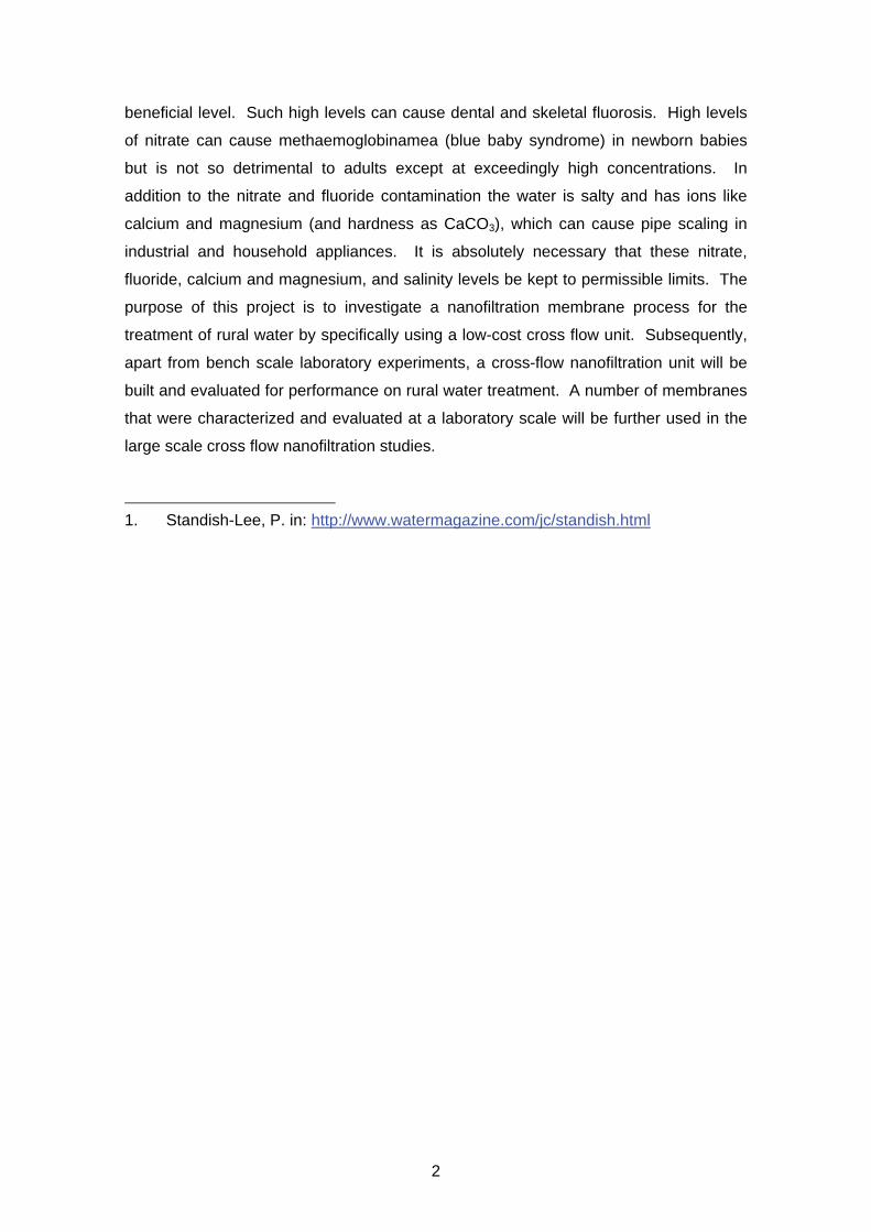
beneficial level. Such high levels can cause dental and skeletal fluorosis. High levels
of nitrate can cause methaemoglobinamea (blue baby syndrome) in newborn babies
but is not so detrimental to adults except at exceedingly high concentrations. In
addition to the nitrate and fluoride contamination the water is salty and has ions like
calcium and magnesium (and hardness as CaCO3), which can cause pipe scaling in
industrial and household appliances. It is absolutely necessary that these nitrate,
fluoride, calcium and magnesium, and salinity levels be kept to permissible limits. The
purpose of this project is to investigate a nanofiltration membrane process for the
treatment of rural water by specifically using a low-cost cross flow unit. Subsequently,
apart from bench scale laboratory experiments, a cross-flow nanofiltration unit will be
built and evaluated for performance on rural water treatment. A number of membranes
that were characterized and evaluated at a laboratory scale will be further used in the
large scale cross flow nanofiltration studies.
1. Standish-Lee, P. in: http://www.watermagazine.com/jc/standish.html

3
2 Literature review
2.1 Nanofiltration – Historical background
Filtration is one of the ancient methods used for water treatment. Sir Francis Bacon,
the philosopher, already used filtration in the 17th century to purify water. Water
filtration for an entire town was in operation in 1804 in Praisley, Scotland. Due to these
successful developments, a large water treatment plant was commissioned (in 1806) in
Paris, using the River Seine as source. In this plant, water was settled for 12 hours
prior to filtration then run through sponge pre-filters that were renewed every hour. The
filters consisted of sand and charcoal [1].
In the late 1800’s, filtration was for the first time recognised not only for straining
unwanted particles, but also for removing deadly germs. During this period, rapid sand
filters were developed, enabling further reduction in turbidity and bacteria. In the
1920’s and 1930’s the use of filtration and chlorination had virtually eliminated
epidemics of major water-borne diseases such as typhoid and cholera. It was within
these two decades that the dissolved air flotation, early membrane filters (primarily for
analytical use), floc-blanked sedimentation and the solid-contact clarifiers were
developed. A major step towards desalination came in the 1940’s during the Second
World War when various military establishments required water to supply troops in arid
regions [2].
Presently, filtration processes are still in use and are continually being refined as more
and better understanding of the complex web of physical and chemical interactions of
the processes (filtration) come to the fore. Particles can now be measured in microns,
compounds in parts per billion and parts per trillion levels. Regulations now require
careful control of by-products of disinfecting processes. As a result, membrane filters
are starting to provide the same and even better purification than conventional water
treatments [1]. The latest of these membrane filtration technologies is nanofiltration
(NF).
In 1988 Eriksson (of FilmTec® Corporation in Minneapolis, USA) was one of the first
authors to toss the word “Nanofiltration” [3] and further gave a broad overview of the
process as well as some applications of NF. NF was defined as a pressure driven
membrane process between reverse osmosis (RO) and ultrafiltration (UF). It gives low
4
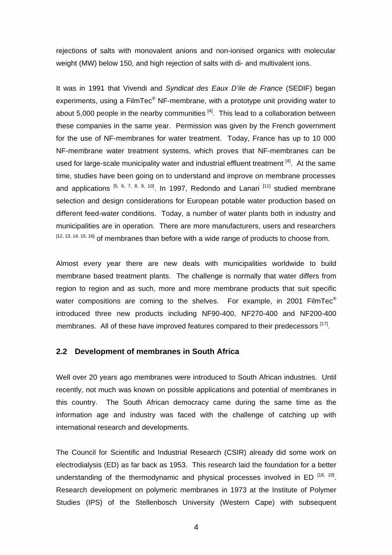
rejections of salts with monovalent anions and non-ionised organics with molecular
weight (MW) below 150, and high rejection of salts with di- and multivalent ions.
It was in 1991 that Vivendi and Syndicat des Eaux D’ile de France (SEDIF) began
experiments, using a FilmTec® NF-membrane, with a prototype unit providing water to
about 5,000 people in the nearby communities [4]. This lead to a collaboration between
these companies in the same year. Permission was given by the French government
for the use of NF-membranes for water treatment. Today, France has up to 10 000
NF-membrane water treatment systems, which proves that NF-membranes can be
used for large-scale municipality water and industrial effluent treatment [4]. At the same
time, studies have been going on to understand and improve on membrane processes
and applications [5, 6, 7, 8, 9, 10]. In 1997, Redondo and Lanari [11] studied membrane
selection and design considerations for European potable water production based on
different feed-water conditions. Today, a number of water plants both in industry and
municipalities are in operation. There are more manufacturers, users and researchers [12, 13, 14, 15, 16] of membranes than before with a wide range of products to choose from.
Almost every year there are new deals with municipalities worldwide to build
membrane based treatment plants. The challenge is normally that water differs from
region to region and as such, more and more membrane products that suit specific
water compositions are coming to the shelves. For example, in 2001 FilmTec®
introduced three new products including NF90-400, NF270-400 and NF200-400
membranes. All of these have improved features compared to their predecessors [17].
2.2 Development of membranes in South Africa
Well over 20 years ago membranes were introduced to South African industries. Until
recently, not much was known on possible applications and potential of membranes in
this country. The South African democracy came during the same time as the
information age and industry was faced with the challenge of catching up with
international research and developments.
The Council for Scientific and Industrial Research (CSIR) already did some work on
electrodialysis (ED) as far back as 1953. This research laid the foundation for a better
understanding of the thermodynamic and physical processes involved in ED [18, 19].
Research development on polymeric membranes in 1973 at the Institute of Polymer
Studies (IPS) of the Stellenbosch University (Western Cape) with subsequent

5
establishment of the first local membrane manufacturing company in 1979 are some of
the important highlights [20]. Currently, membrane research and development are being
pursued at all fronts by educational institutions and private companies, including the
water and power supply institutions.
Some developments recorded include:
Development of woven fibre MF by the Pollution Research Group (University of
Natal, KwaZulu-Natal) in 1980 [21],
Advanced research on cost-efficient manufacture of ozone using membranes and
anode oxidation (University of Western Cape and IPS,
Western Cape) [22],
Extraction of metals by encapsulated supported liquid membranes (SLM)
(Potchefstroom University, North West) [23],
UF membrane bioreactors (IPS, Potchefstroom University and Rhodes University),
Membrane fouling centering around electromagnetic, enzymatic, and chemical
defouling, and surface modifications (Universiy of Stellenbosch, IPS, University of
South Africa) [24, 25],
Development of ceramic membranes by the Separation Science and Technology
(Membrane Group) (Potchefstroom University, North West) [26].
Weir-Envig, a South African membrane company, has designed, manufactured and
commissioned water treatment plants for both private and public sectors since 1985.
Their work included desalination of brackish water and cooling tower blowdown (Sun
International, Dept. Water Affairs, Bateman, Clover SA, ESKOM, Impala, Polifin, etc.),
clarification and concentration of agricultural products e.g. juice, wine, etc. (SFW, CFI,
KWV, Gilbeys’, etc.), paper mill effluent treatment (Mondi paper), etc. [27].
It is the combination of these technological advances and the shortage of drinkable
water that makes the treatment of South African rural water more urgent than before.
Techniques have already been researched but need to be adapted and developed
within the South African context so as to attain this goal.
6
2.3 Membrane processes
A membrane is a selective barrier between two phases. A membrane process is a unit
operation which selectively divides a feed stream into two streams (the retentate and
permeate). The retentate has a higher concentration of the entities retained by the
membrane than the feed, while the other outlet stream, the permeate, has a lower
concentration of the entities held back by the membrane than the feed.
Energy has to be added to the unit operation (membrane process) in order to yield a
separation. This energy input, called the driving force, can be used (in a broad sense)
as a means of classification of membrane processes. The driving force can be any of
the following [28]:
pressure gradient (P),
concentration gradient (c),
temperature gradient (T), or
electrical potential gradient (E).
2.4 Pressure driven processes
There are five pressure driven membrane processes, namely microfiltration (MF),
ultrafiltration (UF), nanofiltration (NF), reverse osmosis (RO) and particle filtration. The
latter is not necessarily seen as a classical membrane operation. RO-membranes,
which are the least permeable, are used for desalination. The disadvantage, however,
is their high operational pressure. Microfiltration membranes are usually porous and
are used for the removal of very small particles, for example during the clarification of
fruit juices. Ultrafiltration gives a rejection of macromolecules (for example the removal
of colour from dye solutions). Nanofiltration membranes are more loose in their
polymer structure than RO-membranes, but have a dense top-layer. The membranes
discriminate between monovalent and multivalent ions as separation takes place on the
basis of both charge and particle size [29, 30].
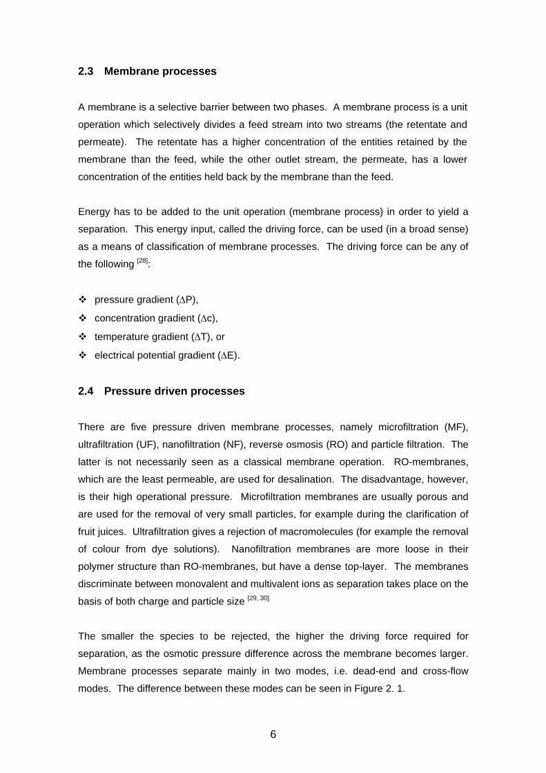
The smaller the species to be rejected, the higher the driving force required for
separation, as the osmotic pressure difference across the membrane becomes larger.
Membrane processes separate mainly in two modes, i.e. dead-end and cross-flow
modes. The difference between these modes can be seen in Figure 2. 1.

7
Figure 2. 1 Dead-end (A) and cross-flow (B) membrane processes
The dead-end mode (marked A) has its feed perpendicular to the membrane and as a
result the retentate builds up on the membrane surface. This might lead to cake
formation or fouling of the membrane surface due to pore clogging or increased
adsorption. In the cross-flow mode (marked B) the feed flows parallel to the membrane
surface, thereby decreasing the fouling or cake formation on the membrane surface.
As a result, cross-flow can have longer sustained fluxes than the dead-end mode of
transport.
2.5 Fouling
During NF, concentration polarization (CP) occurs when the solute is largely rejected
by the membrane. As shown in Figure 2. 2, dissolved species are transported towards
the membrane surface by convective flow during filtration. Water and species smaller
than the pore radius will transport through the membrane whilst larger species are
retained. As these retained species build up on the surface and membrane interface,
their concentration increases until it is higher than that of the bulk stream providing a
driving force for diffusion back into the bulk stream. This build-up at the interface is
known as concentration polarization.
This polarization can be reduced by operating the system at high cross-flow velocities,
so as to increase the shear rate at the membrane interface [31].
feed pressure feed pressure
Dead-end permeate Cross-flow permeate
A B

8
Figure 2. 2 The concentration polarization phenomenon
An irreversible or not easily reversible deposition or binding of solute or particulate onto
or within the membrane is known as fouling. This results in a loss of solvent flux over
time and a change in solute rejection influenced by concentration polarization (CP).
This common problem of flux decline and fouling has direct implications on costs,
energy and the environment during operation.
Foulants include inorganic scalants, suspended solutes and colloidal matter, metal
oxides, organic matter as well as biological material [32, 33, 34]. Fouling can be divided
into several phases [35, 36, 37] which result from concentration polarization, pore blocking
and adsorption of hydrophobic species onto the membrane [38, 39].
Pore blocking is another fouling phenomenon (Figure 2. 3). Pores may either become
clogged when species smaller than their size adsorb onto the inner walls. Chemical
cleaning in place (CIP) is not very effective in removing this adsorbed material on the
inside of the pores and may lead to irreversible fouling.
boundary layer
diffusive transport
convective transport
membrane
cake
Cbulk feed flow
Cwall
permeate flux

9
Figure 2. 3 Pore blocking mechanisms (A: complete pore blocking, entrance to
pore sealed, B: pore bridging: partial obstruction to entrance, C: internal pore
binding, entrapment/adsorption of non-retained species), D: lateral cake
formation (Adapted from Jacobs et al [31])
Apart from fouling, scaling can also occur on the membrane surface. Scaling entails
the precipitation of dissolved salt in the feed water due to the increase in concentration
on the adsorbent surface due to CP. This happens as soon as salts exceed their
solubility product and precipitate. Compounds with a low solubility commonly present
in feed water are calcium carbonate, barium sulfate, silica and calcium phosphate [40].
When scaling occurs, the permeability of the membrane decreases and the head-loss
in the feed-brine channel increases. A higher feed pressure is usually applied to
maintain the desired flux, causing an increase in energy consumption. Even under
these conditions, scaling would still continue causing a further decrease in flux while
simultaneously shortening the life expectancy of the membrane.
There are two causes of flux decline during scale formation in RO; cake formation and
surface blockage [41, 42, 38]. During cake formation, crystal particles, which are formed in
the bulk phase; through bulk (homogenous) or secondary crystallization, are deposited
on the membrane to form a layer. Accumulation of this porous layer precipitate causes
flux decline which can be described by a resistance-in-series model (Equation 2.1):
)( cm RR
PJ
(2. 1)
A B C D
nuclei particle
bulk crystallization
surface crystallization
10
where P is the trans-membrane pressure (bar), is the osmotic pressure difference
(bar), is the permeate viscosity, Rm the membrane resistance and Rc the resistance
due to cake formation.
Surface blockage can also occur due to (heterogeneous) crystallization on the
membrane surface with the subsequent blockage of the membrane by lateral growth of
crystals (Figure 2. 3 D). As the solute (retentate) becomes saturated, it crystallizes in
the bulk solution to form nuclei, which nucleate into particles that precipitate onto the
membrane surface to form a porous cake. Some of the saturated solute precipitates
on the membrane surface and crystallizes. These crystals grow into an impermeable
layer (cake) which subsequently blocks the membrane pores.
Hydrophobic species present in the process water tend to adsorb on hydrophobic
membranes. These species form a layer on the membrane surface that cannot be
removed hydrodynamically, leading to a flux reduction with time. In this case CIP can
initially restore the membrane performance.
In general, fouling (and scaling) control is important as it results in increased energy
consumption, decreased salt rejection and high cleaning frequency which may shorten
the life time of the membrane [43, 44].
2.6 Summary and conclusion
The shortage of water in many parts of the country and the need for strategic water
reuse and management, makes membrane application a necessity for supplementing
current water treatment techniques. Currently however, there is a pressing need to
make clean water available to the rural poor, who largely depend on the extraction of
groundwater for domestic use and farming. The backlog in the usage of this water
source in some areas is caused by the high pollutant content (nitrate and fluoride).
This problem is intense in the Rustenburg area of the North West Province and the far
regions of the Limpopo Province where the levels are unacceptably high. These
pollutants can possibly be reduced to acceptable levels using the nanofiltration
membrane process.
Although nanofiltration is a relatively new membrane process, it has already been
widely applied specifically for water treatment in developed countries (European, Israel
11
and the United States of America) [45, 46, 47]. Research is ongoing in an attempt to
model varying parameters involved during the membrane process (e.g. transport
modeling, adsorption on surface, etc.) [48, 49, 50]. It is attempted to improve on the
membrane products, efficiency and applicability of the membranes. Although there
had been developments in membrane manufacturing in South Africa, there has been
no commercial application and use. The potential of the nanofiltration process to
reduce fluoride and nitrate results from the membrane surface charge that can repel or
attract ions depending on their charge and valence. This is apart from the exclusion of
the solutes based on their molecular sizes. These exclusion properties are as a result
of electrostatic repulsion between the charged membrane and the solute. Retention of
fluoride, nitrate and/or sulfate is dependent on the charge effects. The monovalent
ions are less effectively repelled than the di- and trivalent ions of the same sign of
charge. In NF, retention is also influenced by the co-ion which will be repelled by the
membrane of the same charge.
1. http://www.webster.wrb.stat.ri.us/programs/eo/historydrinkingwater.htm
2 http://www.webster.wrb.stat.ri.us/programs/eo/historydrinkingwater.htm
3. Eriksson, P. (1988) Nanofiltration extends the range of membrane filtration.
Environmental Progress, 7 (1): 58-62.
4. www.dow.com/liquidseps/news/20000926a.html
5. Gould, C. (1995) Treating industrial water with membrane technology. Separation
and Filtration Systems (http://www.osmonics.com).
6. Pickering, K., Wiesner, M.R. (1993) J. Environm. Engineering, 119 (5): 772 –
797.
7. Wiesner, M.R., Sethi, S., Hackney, J., Jacangelo, J. and Lamné, J.M. (1994) J.
Am. Water Works Assoc. 86 (12): 33 – 41.
8. Nafao, S. and Gakkaishi, K. (1995) Current status of membrane separation
separation technology and its future. J. Membrane Science, 18 (2), 66 – 73.

12
9. Shoichi, K., Yasumoto, M., Masaki, I. and Osamu, T. (1995) A corporative study
on the application of the membrane technology on public water supply. J.
Membrane Science, 102 (1-3): 149 – 154.
10. Aron, A. (1996) Membrane technology in water treatment and environmental
protection. Filtration Separation, 33 (6): 459 – 462.
11. Redondo, J.A., and Lanari, F. (1997) Membrane selection and design
considerations for meeting European potable water requirements. Desalination,
113: 309 – 323.
12. Peters, T.A. (1998) Purification of landfill leachate with reverse osmosis and
nanofiltration. Desalination, 119: 289 – 293.
13. Fane, A.G. (1996) Membranes for water production and wastewater reuse.
Desalination, 106: 1 – 9.
14. Wiesner, M.R. and Chellan, S. (1999) The promise of membrane technology.
Environm. Science Technol. 33 (17): 360.
15. Afonso, M.D. and de Pinho, M.N. (2000) Transport of MgSO4, MgCl2 and
Na2SO4 across an amphoteric nanofiltration membrane. J. Membrane Science,
179: 137.
16. Choi, S., Yun, Z., Hong, S. and Ahn, K. (2001) The effect of co-existing ions and
surface characteristics of nanomembranes on the removal of nitrate and fluoride.
Desalination, 133: 53.
17. http://www.dow.com/liquidseps/news/20010304a.html
18. Offringa, G. (2000) Membrane development in South Africa. Membrane
Technology, 119: 4 – 7.
19. Wilson, J.R. (Ed.) Demineralization by electrodialysis. Butterworth Scientific
Publications, London.

13
20. WRC 25 Years 1971-1996 (1996) SA Waterbulletin. Water Research
Commission, South Africa.
21. Pillay, V.L. (1998) Development of cross-flow microfilter for rural water supply.
WRC report No. 386/1/98, Water Research Commission, South Africa.
22. Bessaradov, D.G. (1999) Membranes help to produce high-concentration ozone:
New challenges. Membrane Technology, 114: 5 – 8.
23. Smith J.J. and Koekemoer, L.R. (1996) The extraction of nickel with the use of
supported liquid membrane capsules. Water SA 22 (3): 249 – 256.
24. Leukes, W.D. Buchanan, K. and Rose P.D. (1999) Defouling of ultrafiltration
membranes by linkage of defouling enzymes to membranes for the purpose of
low-cost, low maintenance ultrafiltration of river water. WRC report No. 791/1.99,
Water Research Commission, South Africa.
25. Maartens, A., Swart, P., Jacobs, E.P. (1999) Feed-water and membrane
pretreatment: methods to reduce fouling by natural organic matter. J. Membr.
Sci., 163: 51 – 62.
26. Krieg, H.M., Breytenbach, J.C., and Keizer, K. (2000) Chiral resolution by -
cyclodextrin polymer-impregnated ceramic membranes. J. Membr. Sci,. 164: 177
– 185.
27. http://www.weirenvig.co.za/projects.htm
28. Mulder, M. (1997) Basic principles of membrane technology (2nd ed.). Kluwer
Academic Publishers, Dordrecht.
29. Visser, T.J.K. (2000) Performance of nanofiltration membranes for the removal of
sulphates from acidic solutions. M.Eng. Thesis, Potchefstroom University for
CHE, South Africa.
30. Visser, T.J.K., Modise, S.J., Krieg, H.M. and Keizer, K. (2000) The removal of
acid sulphate pollution by nanofiltration. Desalination, 140: 79 – 86.

14
31. Jacobs, E.P., Pillay, V.L., Pryor, M. and Swart, P. (2000) Water supply to rural
and peri-urban communities using membrane technologies. WRC report no.
764/1/00. Water Research Commission, South Africa.
32. Speth, T.F., Gusses, A.M. and Scott Summer, R. (2000) Evaluation of NF
pretreatments for flux loss control. Desalination, (130): 31 – 44.
33. Osta, T.K. and Bakheet, L.M. (1987) Pretreatment system in reverse osmosis
plants. Desalination 63: 71 – 80.
34. Baker, J., Stephenson, T., Dard, S. and Côté, P. (1995) Characterization of
fouling of nanofiltration membranes used to treat surface waters. Envir. Techn.
16: 977 – 985.
35. Flemming, H.C. and Schaule, G. (1988) Biofouling on membrane – a microbial
approach. Desalination, 70: 95 – 119.
36. Winfield, B.A. (1979) The treatment of sewage effluents by reverse osmosis – pH
based studies of the fouling layer and its removal. Water Resources, 13: 561 –
564.
37. Winfield, B.A. (1979) A study of factors affecting the fouling of reverse osmosis
membranes treating secondary sewage effluents. Water resources, 13: 565 –
570.
38. Lee, S., Kim, J. and Lee, C-K. (1999) Analysis of CaSO4 scale formation
mechanism in various nanofiltration modules. J. of Membrane Science, 163: 63 –
74.
39. Van der Graaf, J.H.J.M., and Roorda, J.H. (October 2000) New developments in
upgrading waste-water treatment plant effluent using ultrafiltration. Membrane
Technology, (126): 4.
15
40. van de Lisdonk, C.A.C., Paassen, J.A.M. and Scippers, J.C. (2000) Monitoring
scaling in nanofiltration and reverse osmosis membrane systems. Desalination,
132: 101 – 108.
41. Gilbron, J. and Hasson, D. (1987) Calcium sulphate fouling of reverse osmosis
membranes: flux decline mechanism. Chem. Engin. Science, 42: 2351 – 2360.
42. Pervov, A.G. (1991) Scale formation prognosis and cleaning procedure
schedules in reverse osmosis systems operation. Desalination, 83: 77 – 118.
43. Bonne, P.A.C., Hofman, J.A.M.H. and van der Hoek, J.P. (2000) Scaling control
of RO membranes and direct treatment of surface water. Desalination, 132: 109.
44. Darton, E.G. (2000) Membrane chemical research: centuries apart. Desalination,
132: 121 – 131.
45. Pahwa, M. and Maheshwari, R.C. Potential of membrane separation technology
forfluride removal from underground water in:
http://envisjnu.tripod.com/newslet/v8nl/model.html
46. Chellam, S. and Sharma, S. (2001) Quality membrane treatability of the lake
Houston Water Supply (Fina Report). The Texas Water Resource Institute,
Technical report 186, Texas.
47. Madireddi, K., Levine, B., Kim, J.H. and Stenstrom, M.K. Dual membrane
separation for removal of organics and dissolved solids during municipal
wastewater reclamation for indirect potable reuse in:
http://www.seas.ucla.edu/stenstro/
48. Nyström, M., Tenninen, J. and Meinttan, M. (2000) Separation of the metal
sulfate and nitrate from their acid using nanofiltration, Membrane Technology,
117: 5 – 9.
49. Ceveal, J.N., Suratt, W.B. and Burke, J.E. (1995) Nitrate removal and water
quality improvement with reverse osmosis for Brighton. Colorado Dessitation,
103: 101 – 112.
16
50. Croll, B.T. and Squires, R. (1993) Exxchange: Dynamic membrane process for
removal of iron, manganese and nitrate from water. Proc. Membr. Technol. Conf.,
553 – 567.

17
3 Dead-end NF and preliminary tests
3.1 Filtration set-up
The bench-scale unit was built (courtesy of Twente University, Henk Veldhuis) to allow
the solution through the top opening or feed inlet as shown in Figure 3.1. A membrane
of a required diameter (9.0cm) is cut and placed at the bottom of the unit on a porous
support. After sealing the unit, it is pressurised up to 20 bar.
The solution (~1.2 litres) is then stirred with a free rotating magnetic bar propelled by
the magnetic stirrer (field). The permeate through the membrane (A = 64cm2) was
collected with plastic sample beakers whilst monitoring the mass flux with the help of a
weighing pan.
Safety valve
Permeate outlet
Membrane onsupport
Diameter = 9 cm
Magnetic stirrer
Feed solution
Pressure inlet Feed inlet
Height = 19 cm
Safety valve
Permeate outlet
Membrane onsupport
Diameter = 9 cm
Magnetic field
Feed solution
Pressure inlet Feed inlet
Height = 19 cm
Figure 3. 1 The high-pressure dead-end module

18
3.2 Membranes
The NF-membranes of different specifications (Table 3. 1) used in this study were
obtained from different manufacturers. These polymeric membranes were supplied as
flat sheets, except for the NF70 and NF90, which were spiral-wound and thus had to be
unwound and cut to flat sheets. The membranes used were:
D11 and D12 from MembraTek-Envig South Africa,
NF70 and NF90 from Dow – FilmTec®,
TFC-S, TFC-SR, and TFC-HR from Koch Membrane Systems, and
CTC1 (Chlorine tolerant membrane) from Hydranautics.
Table 3. 1 Specifications of NF-membranes
D11 D12 NF70 NF90 CTC1 TFC-S TFC-SR TFC-HR
MWCO (Da) 180 180 200 – – – – –
NaCl (%) 50 15 – – 90e 85c 30c 99.5
MgSO4 (%) 96a 96a 95b 96b – 95d 98.5d –
Design- or pressure range (bar)
5 – 28 5 – 28 17 17 41.6 4 – 7 5 15
Max. temp (oC) 50 50 35 35 45 45 45 45
pH range 4 – 11 4 – 11 3 – 9 3 – 9 3 – 10 4 – 11 4 – 11 4 – 11
Flow (m3.d-1) 7.6 f 10.6g 3.2g 2.5g 0.3g – – –
a: 1000ppm solute at 6.9bar net pressure; b: <2000ppm solute, at 5bar, pH = 7 and 25oC; c:
1000ppm solute, 6bar, pH = 7 and 25oC; d: 2500ppm solute, 6bar, pH = 7 and 25oC; e: 500ppm
solute at 4.5bar applied pressure, pH = 6.5-7.0 and 25oC; f: model D11 4040 element, g: 2540
elements, area = 2.6m2.
The Envig (D11 and D12) membranes are both thin film composite membranes with
the molecular weight cut-off range well within that of nanofiltration membranes. The
NF70 and NF90 are composite membranes. NF70 has a negative charge at high pH
values due to the dissociation state of the amine groups in the thin layer [1]. TFC-S is a
thin layer composite polyamide membrane on a polysulfone base. It is usually stored
these membranes were donated courtesy of the manufacturers

19
wet in a dark area and must be “cleaned” or pretreated before use. TFC-SR is a thin-
film composite propriety membrane on a polysulfone base. It is supplied dry with a
poly(vinyl)alcohol (PVA) coating which has to be removed by washing or water
permeation before use. TFC-HR is also a thin-film polyamide membrane on a
polysulfone base. It is stored dry and also has a PVA coating. CTC1 is a thin layer
composite polyamide membrane.
All the membranes were pretreated by flushing the membrane with feed in situ, sending
the permeate to drain for about 10min or until the permeate was clear.
3.3 Permeation measurements
There are various variables that have an influence on the performance of a membrane.
Normally, a compromise is struck between the retention capacity and the flux of a
membrane. Although a high retention and flux are desirable, the two parameters
(retention and flux) are antagonistic, with high fluxes yielding low retention and vice
versa. The volume fluxes are influenced by the applied pressure while the solute fluxes
are proportional to the concentration gradient.
There is also the sterical hindrance of solutes that are transported through the
membrane pores, which is dependent on the molecular weight and ionic charge and
size of the transported solutes. This means that solutes will be discriminated based on
their molecular sizes as well as on their ionic charge in case of electrolytes. Larger
molecules will be rejected while the smaller ones are transported through the
membrane “pores” to the permeate phase.
3.3.1 Clean water flux
Clean water (demineralized) is used as a reference in membrane characterization
since charge or concentration polarisation and/or molecular weight have no effect on
the flux. The water flux (Jw) is measured at various trans-membrane pressure
differences (TMP) to yield the water permeability (AW or Lp in L.m-2.s-1.bar-1 or
m.s-1.bar-1). This relation is best described by the Hagen-Poiseuille Equation:
x
PrJw
.
8
2
(3. 1)
20
where Jw is the water flux (in m.s-1 or L.m-2.hr-1), is the porosity, r is the pore radius (in
m), is the tortuosity (indicative of how straight the pores are, equals one when the
pores are straight), is the viscosity of water (in Pa.s), x is the membrane thickness
(in m) and P is the applied trans-membrane pressure (in kPa).
The linear relationship between flux and pressure is indicative of a constant
permeability for every membrane. The water flux can be described according to the
model of Darcy [2]:
PAJ ww (3. 2)
Since both the feed and permeate of the membrane consist of water, the osmotic
pressure difference () across the membrane is zero and Equation (3. 2) is reduced
to:
PAJ ww (3. 3)
which is comparative to the Hagen-Poiseuille model.
Combining Equations (3. 1) and (3. 3), Equation (3. 4) is obtained:
x
rAw
8
2
(3. 4)
where
xP
(3. 5)
is the tortuosity (-) with p the real length of the pore (in m) and x the membrane
thickness (in m). Tortuosity equals one if both x and p are the same, which means
that the pores are perpendicular to the membrane surface.
21
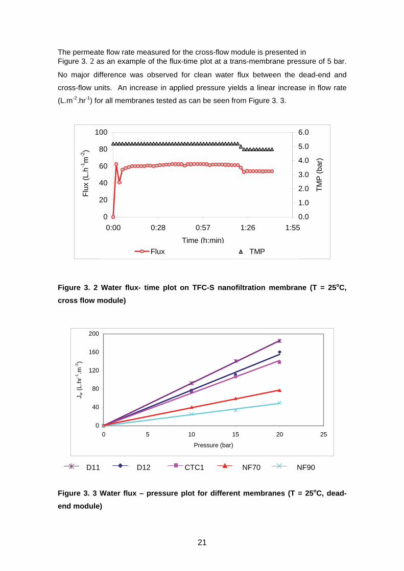
The permeate flow rate measured for the cross-flow module is presented in Figure 3. 2 as an example of the flux-time plot at a trans-membrane pressure of 5 bar.
No major difference was observed for clean water flux between the dead-end and
cross-flow units. An increase in applied pressure yields a linear increase in flow rate
(L.m-2.hr-1) for all membranes tested as can be seen from Figure 3. 3.
0
20
40
60
80
100
0:00 0:28 0:57 1:26 1:55
Time (h:min)
Flu
x (L
.h-1
m-2
)
0.0
1.0
2.0
3.0
4.0
5.0
6.0
TM
P (
bar)
Flux TMP
Figure 3. 2 Water flux- time plot on TFC-S nanofiltration membrane (T = 25oC,
cross flow module)
0
40
80
120
160
200
0 5 10 15 20 25
Pressure (bar)
J w (
L.hr
-1.m
-2)
D11 D12 CTC1 NF70 NF90
Figure 3. 3 Water flux – pressure plot for different membranes (T = 25oC, dead-
end module)

22
When it is approximated that
1 then
wAxr 82 (3. 6)
The value of Aw is obtained experimentally from the slope of the plot of volume flux
(L.m-2.hr-1) versus pressure (bar) as in Figure 3. 3. It can be assumed that the viscosity
of pure water is 0.001Pa.s and x is 1m. From the above approximation . r can be
calculated from the water permeability data (Table 3. 2).
Table 3. 2 Clean water permeability and porosity value of NF-membranes
Membrane
type
Aw
(L.m-2.hr-1.bar-1)
.r
(Å)
D11 9.21 4.52
D12 8.79 4.42
CTC1 6.08 3.68
NF70 3.66 2.85
NF90 2.48 2.35
TFC-S 2.04 2.13
TFC-SR 12.0 5.16
TFC-HR 3.45 2.77
The values of water permeability (Aw) and .r are given in Table 3. 2 for the membranes
tested. Two classifications of the membranes can be done; those that have low clean
water permeability between 2 and 3 L.m-2.hr-1.bar-1 (NF70, NF90, TFC-S and TFC-HR)
and those that exceed 6 L.m-2.hr-1.bar-1 (D11, D12, CTC1 and TFC-SR). The latter
suggests that these membranes are more loosely packed while NF70, NF90, TFC-S
and TFC-HR are more tightly packed. The observed water permeability are
proportional to the product (.r)2.
3.4 Nanofiltration of salts
The ability of nanofiltration membranes to reject electrolytes is owed to the Donnan
exclusion effect. During the membrane surface’s contact with electrolytes, co-ions
(those having the same charge as the membrane) and counter-ions are distributed
23
between the membrane and the solution. At this stage, the electrical forces on the
membrane-electrolyte interfaces (feed-membrane and permeate-membrane interfaces)
play an important role in the membrane performance. In the case of salt mixtures, the
diffusion coefficients and the hindrance factors also come into play resulting in the
Donnan equilibrium. These added factors yield improved multivalent rejections.
In this section, the rejection capabilities of the NF-membranes that are used later for
water treatment are presented. The ions (sulfate, chloride and nitrate), both as single
salts and salt mixtures, were used to determine the retention behaviour of the NF70,
NF90, D11, D12, CTC1, TFC-S, TFC-SR and TFC-HR membranes. The effect of pH
on retention was also determined.
3.5 Theory
It was stated before that the properties of NF-membranes are between those of reverse
osmosis and ultrafiltration. The separation by ultrafiltration membranes is largely
influenced by steric effects whilst electric effects influence the reverse osmosis
membrane processes. NF-membranes are influenced by both effects. Separation is
influenced by the physical parameters such as pore radius, membrane thickness and
the electrical charge density on the surface. The overall result is that the NF-
membrane can reject mono- and divalent ions. As complex as the process can be, it
can be explained in terms of theories such as the extended Nernst-Planck model,
charge shielding, Donnan exclusion and the degree of hydration. Modeling of
electrolytes has been done by a number of researchers [3, 4, 5, 6] and will not be dealt
with in this section. Instead, only performance in terms of the rejection coefficient and
flux will be investigated.
3.6 Tests
3.6.1 NF of single salts
The effects of stirring (and speed), concentration and pressure (and flow mode) were
investigated. All the concentrations were monitored by a colorimeter (HACH DR/890),
a conductimeter (HI pH9032) and an IC (Waters Model 510). All experiments were
carried out on CTC1, TFC-S, TFC-SR TFC-HR, NF70 and NF90 membranes on a
dead-end unit, unless otherwise stated.
24
The fluxes of the membranes were first determined using solutions of sodium chloride
(NaCl), sodium sulfate (Na2SO4), calcium chloride (CaCl2), sodium nitrate (NaNO3),
sodium fluoride (NaF), and calcium sulfate (CaSO4). The solutions were prepared at
concentrations of 20, 50, 100 and 200ppm (prepared as anion concentration). The
sulphuric acid concentration (H2SO4) ranged from 50 to 2000ppm as total sulphate
concentration. The pressure applied in all experiments were 5, 10, 15 and 20bar.
Additionally, some experiments at lower trans-membrane pressures (2–6bar) were
carried out for CaSO4, NaNO3, H2SO4, NaCl, Na2SO4 and CaCl2 on NF70, NF90, and
CTC1 membranes.
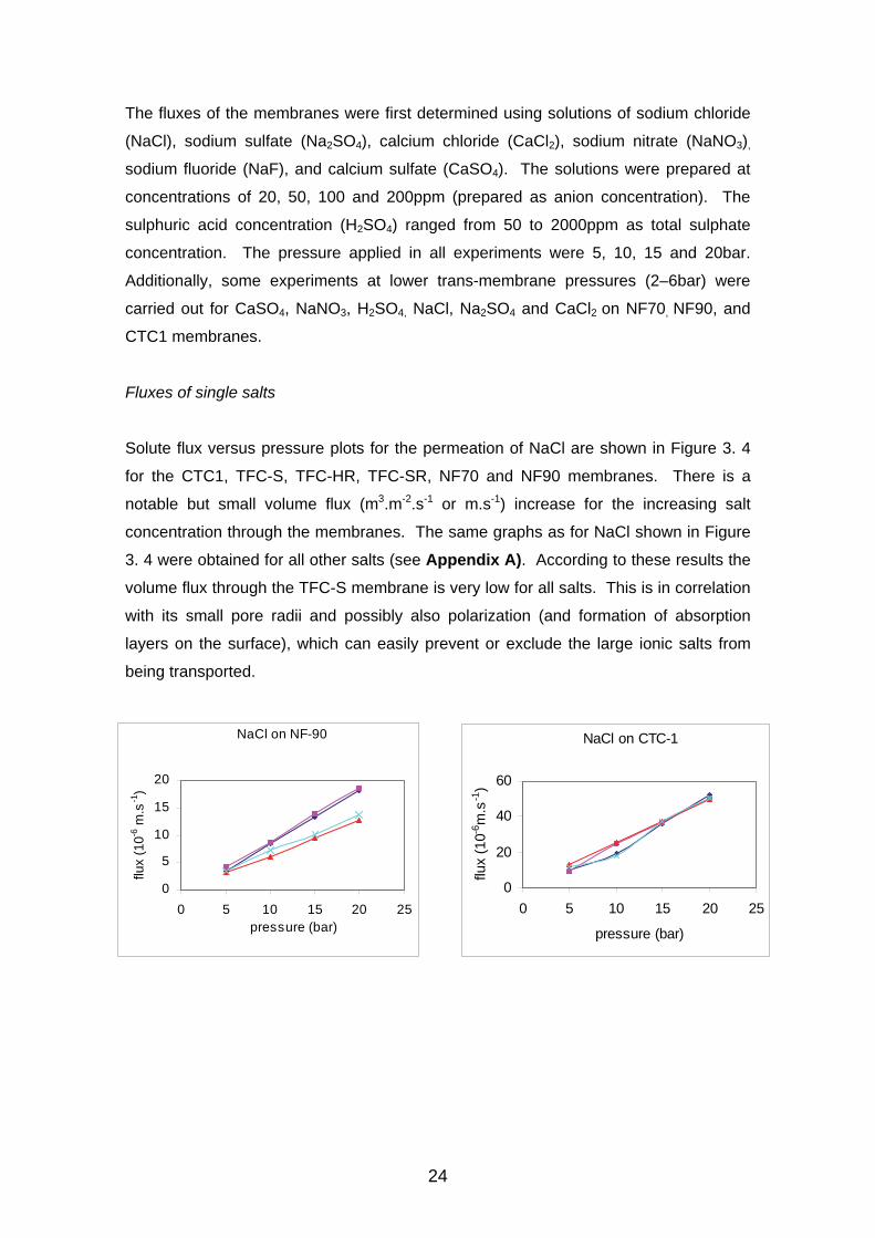
Fluxes of single salts
Solute flux versus pressure plots for the permeation of NaCl are shown in Figure 3. 4
for the CTC1, TFC-S, TFC-HR, TFC-SR, NF70 and NF90 membranes. There is a
notable but small volume flux (m3.m-2.s-1 or m.s-1) increase for the increasing salt
concentration through the membranes. The same graphs as for NaCl shown in Figure
3. 4 were obtained for all other salts (see Appendix A). According to these results the
volume flux through the TFC-S membrane is very low for all salts. This is in correlation
with its small pore radii and possibly also polarization (and formation of absorption
layers on the surface), which can easily prevent or exclude the large ionic salts from
being transported.
NaCl on NF-90
0
5
10
15
20
0 5 10 15 20 25pressure (bar)
flux
(10-6
m.s
-1)
NaCl on CTC-1
0
20
40
60
0 5 10 15 20 25
pressure (bar)
flux
(10-6
m.s
-1)

25
NaCl on NF-70
0
5
10
15
20
0 5 10 15 20 25
pressure (bar)
flux
(10
-6m
.s-1
)
NaCl on TFC-S
0.0
0.2
0.4
0.6
0.8
1.0
0 5 10 15 20 25
pressure (bar)
flux
(10-6
m.s
-1)
NaCl on TFC-HR
0
5
10
15
20
25
0 5 10 15 20 25
pressure (bar)
flux
(10-6
m.s
-1)
NaCl on TFC-SR
0
20
40
60
80
0 5 10 15 20 25
pressure (bar)
flux
(10
-6 m
.s-1
)
0 mg/L 20 mg/L 50 mg/L 100 mg/L 200 mg/L
Figure 3. 4 Solute flux – pressure relations of varying NaCl concentrations
through different membranes (T = 25oC, dead-end mode)
Contrary to TFC-S, TFC-SR has high fluxes in the presence of all salts. Furthermore,
the permeated flux through the membrane is relatively constant for all the salts (1-1
(e.g. NaCl), 2-1 (e.g. CaCl2), and 1-2 (e.g. Na2SO4)). The water flux (Aw in L.m-2.hr-
1.bar-1) shows the same trend as the solute fluxes for the TFC-SR membrane,
indicating that the membrane is equally permeable even for the charged solutes. The
same cannot be said for the CTC1 membrane which has higher water fluxes than
solute fluxes. In general, the concentration polarization is not that severe for the
membranes except for TFC-S and NF90 which show noticeable differences in fluxes,
probably due to surface polarization and restricted pore radii. Solute flux decreases in
the order TFC-SR > CTC1 > NF70, NF90 > TFC-S.
26
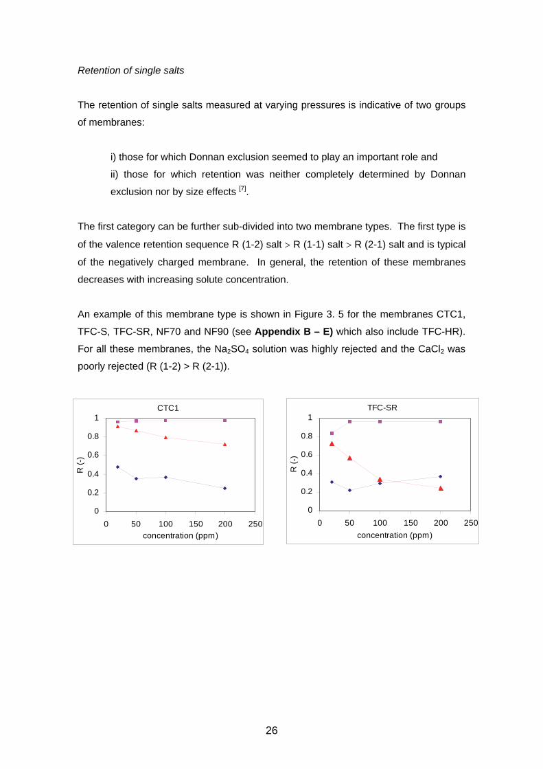
Retention of single salts
The retention of single salts measured at varying pressures is indicative of two groups
of membranes:
i) those for which Donnan exclusion seemed to play an important role and
ii) those for which retention was neither completely determined by Donnan
exclusion nor by size effects [7].
The first category can be further sub-divided into two membrane types. The first type is
of the valence retention sequence R (1-2) salt R (1-1) salt R (2-1) salt and is typical
of the negatively charged membrane. In general, the retention of these membranes
decreases with increasing solute concentration.
An example of this membrane type is shown in Figure 3. 5 for the membranes CTC1,
TFC-S, TFC-SR, NF70 and NF90 (see Appendix B – E) which also include TFC-HR).
For all these membranes, the Na2SO4 solution was highly rejected and the CaCl2 was
poorly rejected (R (1-2) > R (2-1)).
CTC1
0
0.2
0.4
0.6
0.8
1
0 50 100 150 200 250
concentration (ppm)
R (
-)
TFC-SR
0
0.2
0.4
0.6
0.8
1
0 50 100 150 200 250
concentration (ppm)
R (
-)

27
TFC-S
0
0.2
0.4
0.6
0.8
1
0 50 100 150 200 250
concentration (ppm)
R (
-)
NF70
0
0.2
0.4
0.6
0.8
1
0 50 100 150 200 250
concentration (ppm)
R (
-)
NF90
0
0.2
0.4
0.6
0.8
1
0 50 100 150 200 250
concentration (ppm)
R (
-)
Figure 3. 5 Retention versus concentrations of (2-1), (1-1), and (1-2) salts (anions)
The second type of the first category shows the ionic valence retention sequence R (2-
1) salt R (1-1) salt R (1-2) salt, which is a reverse of the first type. This sequence is
typical of positively charged membranes. An example of this type in this category was
however not found among the membranes evaluated.
In Table 3. 3 a summary of the behaviour of membranes in terms of the rejections of
CaCl2, NaCl, and Na2SO4. According to these results, all membranes tend to fall within
the first category. The difference in retention for (2-1) salt and (1-1) salt by NF70,
NF90, TFC-S, and TFC-SR, is statistically not significant in assigning a membrane
surface charge. While NF70, TFC-S, and TFC-SR show a tendency towards
negatively charged membranes, CTC1 gives the typical behaviour of a negatively
charged membrane. NF70 and NF90 showed membrane characteristics that are
Na2SO4 NaCl Na2SO4
28
closer to those of reverse osmosis membranes than NF, as all salts were retained
equally well by these membranes.
Table 3. 3 Single salt retentions of (2-1), (1-1), and (1-2) salts on different
membranes
Single salts retention * (%)
Membrane CaCl2 (2-1) NaCl (1-1) salt Na2SO4 (1-2) salts
NF70 92.3 96.2 99.1
NF90 93.8 91.0 92.7
CTC1 36.4 79.6 97.7
TFC-S 82.7 88.9 97.3
TFC-SR 29.3 33.8 96.2
*at concentration = 20ppm and pressure = 20bar
3.6.2 Salt mixtures
The experiments were done at pressures of 10 and 20bar using mixtures of
CaCl2/CaSO4, CaCl2/CaF2, NaCl/CaCl2, CaSO4/Na2SO4, and NaCl/Na2SO4 on TFC-SR,
NF70 and NF90 membranes. The ion ratios used were 1:9, 3:7, 5:5, 7:3 and 9:1. The
total concentration of the common ion was set to 200ppm. A pH meter (HI pH301),
colorimeter (HACH DR/890), ion chromatography (Water model 510), and atomic
absorption (Varian SpectrAA 250 plus) were used for monitoring the ions. All mixtures
were prepared using demineralized water.
The dead end unit was equipped with a stirrer to maintain the concentration as
homogenous as possible throughout the reactor. The stirrer could be set at low or high
stirring modes. To study the effect of stirring rate on concentration polarization at low
concentration, clean water and a 100ppm solution of CaSO4 was used on a TFC-SR
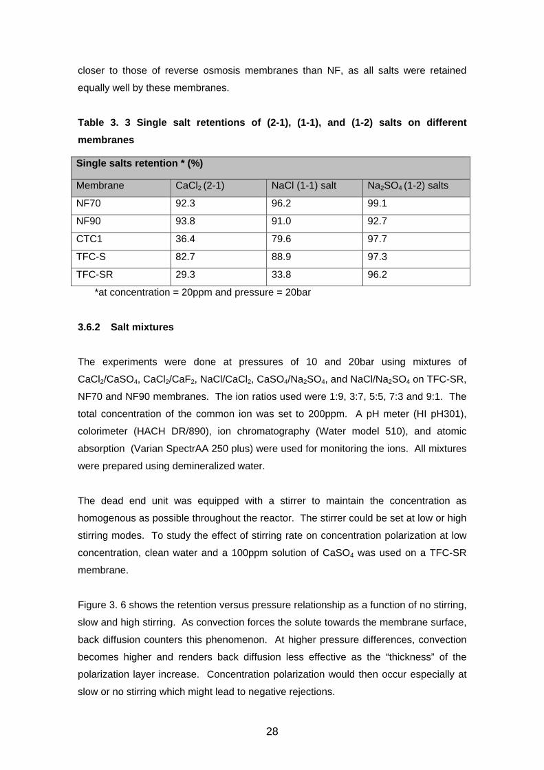
membrane.
Figure 3. 6 shows the retention versus pressure relationship as a function of no stirring,
slow and high stirring. As convection forces the solute towards the membrane surface,
back diffusion counters this phenomenon. At higher pressure differences, convection
becomes higher and renders back diffusion less effective as the “thickness” of the
polarization layer increase. Concentration polarization would then occur especially at
slow or no stirring which might lead to negative rejections.
29
0
0.2
0.4
0.6
0.8
1
0 5 10 15 20 25
pressure (bar)
R(-
)
no stirring slow stirring fast stirring
Figure 3. 6 Retention – pressure relation showing the effect of stirring on TFC-SR
membrane (T = 25oC, dead-end mode)
Stirring (slow/fast) compared to no stirring leads to high rejections but does not
necessarily mean it would completely remove polarisation. Since the solvent
permeates through the membrane, the solute that was formerly dissolved accumulates
on the membrane surfaces. The concentration of the solute then increases, especially
in the boundary layer. The local concentration difference across the membrane would
then increase, ultimately resulting in increased fluxes of the solute through the
membrane.
The flux–pressure relationship for clean water and CaSO4 solution is shown in Figure
3. 7 at varying stirring rates. The solute flux decreases with decreasing stirring rate
while fast stirring improves the solute flux to such an extent that it becomes
comparable to, although somewhat lower than the flux of clean water, which remained
the same regardless of the stirring speed. This is because water has no charged ions
that concentrate on the membrane surface. Therefore, it can be concluded that stirring
is important when using a dead–end mode in order to minimize concentration
polarization.

30
0
20
40
60
80
100
120
0 5 10 15 20 25pressure (bar)
flux
(10
-6m
.s-1)
salt no stirring salt slow stirring salt fast stirring
water no stirring water slow stirring water fast stirring
Figure 3. 7 Flux – pressure relations showing the effect of stirring on TFC-SR
membrane (50ppm CaSO4, T = 25oC, dead-end mode)
A set of salt mixtures were prepared and permeated through all the membranes as with
the single salts.
Retention of NaCl/Na2SO4
These experiments were carried out on TFC-SR, NF70 and NF90. The two former
membranes showed a slight negatively charged behaviour during single (NaCl and
Na2SO4) salt studies and were classified within the first category of the membranes
(Donnan exclusion important). NF90 seemed to reject both divalent anions and cations
equally well, while also retaining NaCl.
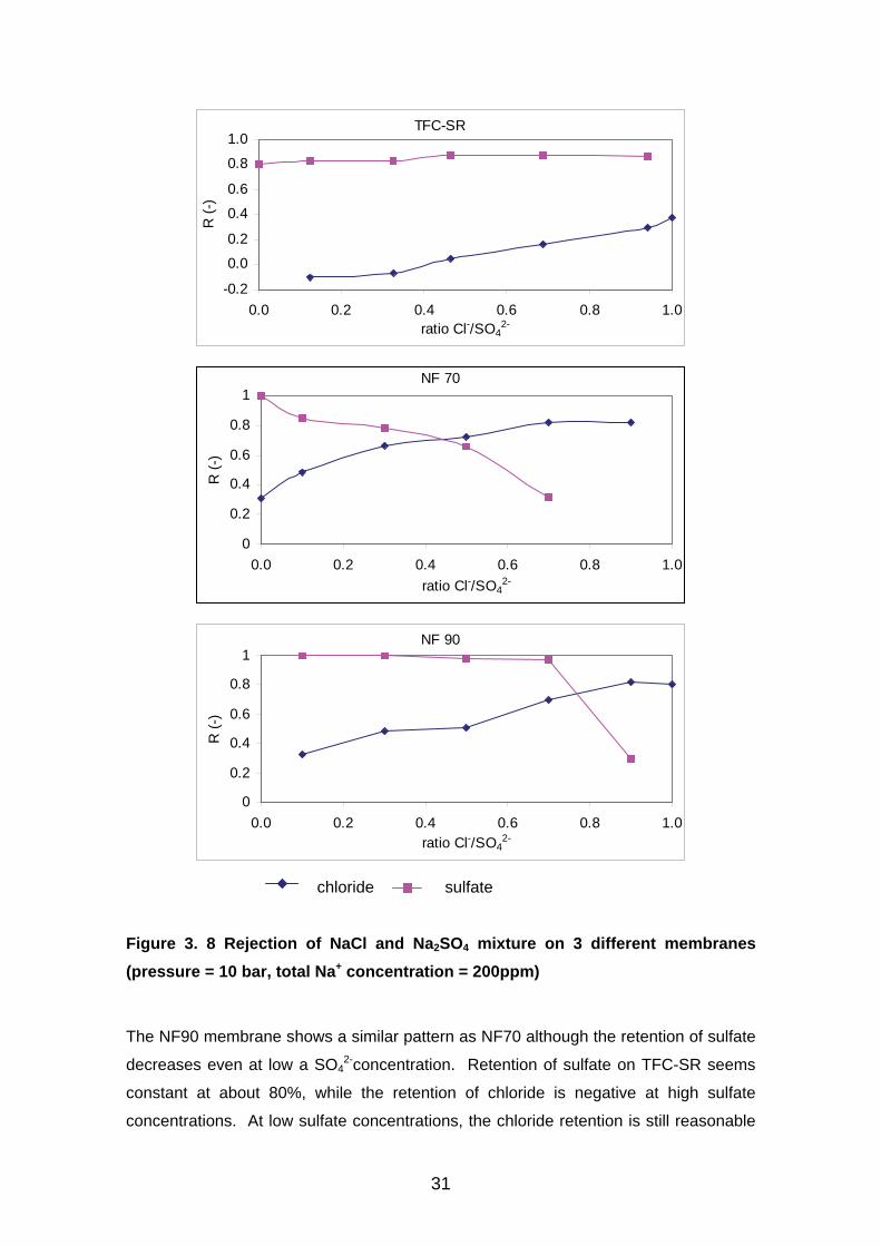
Figure 3. 8 is an example of the retention-ion fraction plot of the NaCl/Na2SO4 mixture
for the three chosen membranes. Except for TFC-SR, the chloride retention decreases
as the concentration of the sulfate increases in the mixture. The implication is that
increasing high valence co-ion (SO42-) concentration will “push” more chloride into the
membrane and decrease its retention while the retention of sulfate would
simultaneously increase. The rejection of the sulfate is depressed by an increasing
chloride concentration in the solution (except for TFC-SR). The reason for this is that
the sulfate concentrations are low at this ratio and their retention is compromised by
the retention of the chlorides.
31
TFC-SR
-0.2
0.0
0.2
0.4
0.6
0.8
1.0
0.0 0.2 0.4 0.6 0.8 1.0ratio Cl-/SO4
2-
R (
-)
NF 70
0
0.2
0.4
0.6
0.8
1
0.0 0.2 0.4 0.6 0.8 1.0
ratio Cl-/SO42-
R (
-)
NF 90
0
0.2
0.4
0.6
0.8
1
0.0 0.2 0.4 0.6 0.8 1.0ratio Cl-/SO4
2-
R (
-)
chloride sulfate
Figure 3. 8 Rejection of NaCl and Na2SO4 mixture on 3 different membranes
(pressure = 10 bar, total Na+ concentration = 200ppm)
The NF90 membrane shows a similar pattern as NF70 although the retention of sulfate
decreases even at low a SO42-concentration. Retention of sulfate on TFC-SR seems
constant at about 80%, while the retention of chloride is negative at high sulfate
concentrations. At low sulfate concentrations, the chloride retention is still reasonable
32
for NF70 and NF90 (~80%), but low for TFC-SR (~30%). This shows that there is little
transport of sulfate into the membrane whilst that of the monovalent co-ion is
increased. In general, the retention of the monovalent co-ion was lower for the salt
mixtures as compared to the single salt studies.
The volume flux (m.s-1) of the mixtures remains constant for increasing ratios but
increases with increasing pressure. For TFC-SR the volume flux was ~22 x 10-6 m.s-1
at 10 bar and ~41 x 10-6 m.s-1 at 20 bar.
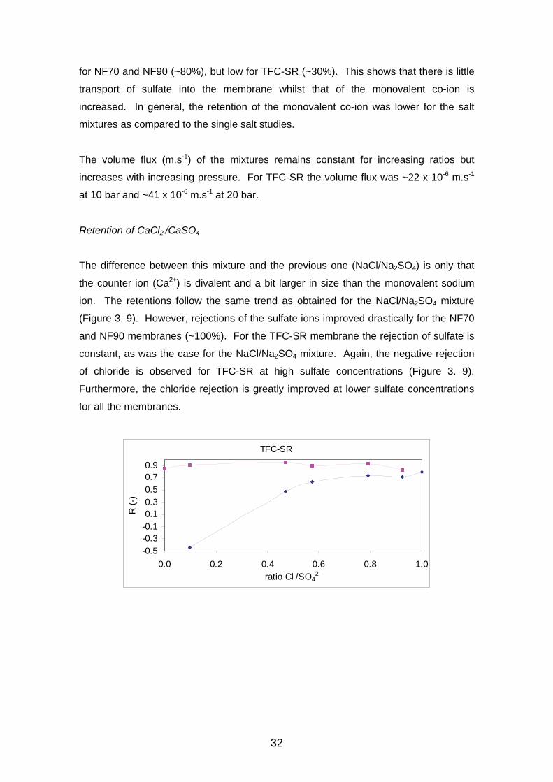
Retention of CaCl2 /CaSO4
The difference between this mixture and the previous one (NaCl/Na2SO4) is only that
the counter ion (Ca2+) is divalent and a bit larger in size than the monovalent sodium
ion. The retentions follow the same trend as obtained for the NaCl/Na2SO4 mixture
(Figure 3. 9). However, rejections of the sulfate ions improved drastically for the NF70
and NF90 membranes (~100%). For the TFC-SR membrane the rejection of sulfate is
constant, as was the case for the NaCl/Na2SO4 mixture. Again, the negative rejection
of chloride is observed for TFC-SR at high sulfate concentrations (Figure 3. 9).
Furthermore, the chloride rejection is greatly improved at lower sulfate concentrations
for all the membranes.
TFC-SR
-0.5-0.3-0.10.10.30.50.70.9
0.0 0.2 0.4 0.6 0.8 1.0ratio Cl-/SO4
2-
R (
-)

33
NF-70
0.0
0.2
0.4
0.6
0.8
1.0
0.0 0.2 0.4 0.6 0.8 1.0ratio Cl-/SO4
2-
R (
-)
NF-90
0.0
0.2
0.4
0.6
0.8
1.0
0.0 0.2 0.4 0.6 0.8 1.0
ratio Cl-/SO42-
R (
-)
chloride sulfate
Figure 3. 9 Rejection of CaSO4 and CaCl2 mixture on 3 different membranes
(pressure = 10 bar, total Ca2+ concentration = 200ppm)
This can be due to the slight impermeability of counter ions, which causes chloride ions
to remain behind on the feed side. This effect ‘costs’ two chloride ions for every
calcium that fails to be transported through the membrane. It seems, however, that this
effect is countered by high sulfate concentrations.
Retention of NaCl/CaCl2
The NF70 and NF90 membranes show almost similar tendencies as with the anionic
co-ion rejections (Cl-/SO42-). The calcium rejection by NF70 and NF90 is about 90%
and remains nearly constant even with increasing calcium concentrations (Figure 3.
10). Contrary to the monovalent anion retention pattern, the monovalent cation
retention is high even at high calcium concentrations. That is, retention does not

34
increase with increasing high valence concentration. This is because the transport of
Na+ is not accelerated resulting from the negative charge of the membrane.
The high retention of both cations (Na+ and Ca2+) by the NF90 membrane results in the
improved rejections of the monovalent anion, which is a co-ion in this case. The
retention of sodium decreases with increasing concentration at low divalent cation
concentrations. This is an opposite effect to a decrease in retention in chlorides at high
divalent cation concentrations. Also, there would be reduced retention of cationic
divalents as compared to the anionic divalents if the NaCl/Na2SO4 or CaCl2/CaSO4
mixture were to be used. The same trend is observed for the NF70 membrane.
The rejection on the TFC-SR shows a similar pattern as in the anionic co-ion retentions
except that rejections here are even lower (not more than 70% for calcium). Calcium
shows a decrease in rejection at low concentrations, increasing at high calcium
concentrations. Again, sodium ions have their rejections reduced at high divalent
cation concentrations. No negative retention was observed though, as seemingly not
much of the sodium is transported into the membrane when using this mixture, owed to
the poor rejection of divalent calcium, even at high concentrations.
TFC-SR
0.0
0.2
0.4
0.6
0.8
1.0
0.0 0.2 0.4 0.6 0.8 1.0
ratio Na+/Ca2+
R (
-)

35
NF-70
0.0
0.2
0.4
0.6
0.8
1.0
0.0 0.2 0.4 0.6 0.8 1.0
ratio Na+/Ca2+
R (
-)
calcium sodium
Figure 3. 10 Rejection of NaCl and CaCl2 mixtures on 3 different membranes
(pressure = 10 bar, total Cl- concentration = 200ppm)
Retention of Na2SO4/Ca2SO4
Figure 3. 11 is a retention-ion fraction plot for the NF70, NF90 and TFC-SR
membranes.
NF-90
0.0
0.2
0.4
0.6
0.8
1.0
0.0 0.2 0.4 0.6 0.8 1.0
ratio Na+/Ca2+
R (
-)

36
TFC-SR
0.5
0.6
0.7
0.8
0.9
1.0
0.0 0.2 0.4 0.6 0.8 1.0
ratio Na+/Ca2+
R (
-)
NF-70
0.5
0.6
0.7
0.8
0.9
1.0
0.0 0.2 0.4 0.6 0.8 1.0
ratio Na+/Ca2+
R (
-)
NF-90
0.5
0.6
0.7
0.8
0.9
1
0.0 0.2 0.4 0.6 0.8 1.0
ratio Na+/Ca2+
R (
-)
calcium sodium
Figure 3. 11 Rejections of Na2SO4 and CaSO4 mixtures on 3 different membranes
(pressure = 10 bar, total SO42- concentration = 200ppm)
The difference between this mixture and the one in the previous section is that the co-
ion is a divalent (SO42-). The NF70 and the NF90 show high rejection of calcium and
the sulfate co-ion. The two membranes show the same behaviour as for the

37
NaCl/CaCl2 mixtures. TFC-SR shows the same behaviour as the NF70 and NF90 also
for the NaCl/CaCl2 rejected ion since the ratio of the counter-ions are similar.
Retention of CaCl2/CaF2
Mixtures of CaCl2/CaF2 were prepared with a maximum concentration of 5ppm calcium
fluoride and calcium chloride due to the low solubility of CaF2, and tested on TFC-SR.
The rejections of both fluoride and chloride were high (80% and 85%, respectively)
irrespective of the Cl-/F- ratio (Figure 3. 12).
TFC-SR
0.0
0.2
0.4
0.6
0.8
1.0
0.0 0.2 0.4 0.6 0.8 1.0
ratio Cl-/F-
R (
-)
chloride fluoride calcium
Figure 3. 12 Rejection of CaCl2and CaF2 mixtures on TFC-SR (pressure = 10 bar,
F- concentration = 5ppm)
This constant rejection may be dependent on electronegativity but not on the ion size
and valence since although chloride has a larger ion radius (1.81 Å) than fluoride (1.33
Å), it is not rejected more. It could be that calcium is not transported through the
membrane, but at the same time it cannot be retained without a neutralising charge.
One could assume that a mixture of NaCl/NaF would probably have reduced rejections
since both the counter-ions (sodium) and co-ions (fluoride and chloride) are
monovalent.
3.7 Summary and conclusion
38
The possible occurrence of concentration polarization can be minimized by stirring at
high speeds. This polarization was evident when there was no stirring or at very low
stirring speeds. This results from the concentration build-up on the membrane surface.
By stirring, the concentration becomes homogenous throughout the feed tank and in
the membrane reactor.
All membranes in this study seem to have a negative membrane surface charge. As a
result, the negatively charged co-ions, especially of high valence are easily retained by
the membrane. Such retention is even more effective at high concentrations of such
divalents. This has been demonstrated by single salt and salt mixture experiments.
The Donnan equilibrium and exclusion plays an important role in the rejections of these
ions.
All membranes, except NF90 were found to fall within the first type of the first category.
For this category and type, the valence retention sequence noticed is R (1-2) > R (1-1)
> R (2-1). The NF90 could not be classified in any of the categories as it rejects ions
equally suggesting that the membrane is amphoteric in nature.
Studies with salt mixtures showed decreased retention for monovalent co-ions but
improved retention for divalent co-ions, especially at high concentrations which will
“push” more monovalents into the membrane, thereby decreasing their retention. The
high valence counter-ions are generally poorly rejected but cause a better rejection of
monovalent co-ions.
1. Visser, T.J.K., Modise S.J., Krieg, H.M. and Keizer, K. (2000) The removal of acid
sulfate pollution by nanofiltration. Desalination, 140: 79 – 86.
2. Mulder, M. (1997) Basic principles of membrane technology. (2nd Ed.), Kluwer
Academic Publishers, Dordrecht.
3. Afonso, M.D., de Pinho, M.N. (2000) Transport of MgSO4, MgCl2, and Na2SO4
across an amphoteric nanofiltration membrane. J. of Membrane Science, 179:
137.

39
4. Choi, S., Yun, Z., Hong, S. and Ahn, K. (2001) The effect of co-existing ions and
surface characteristics of nanomembranes on the removal of nitrate and fluoride.
Desalination, 133: 53.
5. Bowen, W.R., Mohammad, A.W. and Hilal, N. (1997) Characterization of
nanofiltration membranes for predictive purposes – use of salts, uncharged
solutes and atomic force microscopy. J. of Membrane Science, 60: 1811.
6. Linde, K. and Jonsson, A.S. (1995) Nanofiltration of salt solution and landfill
leachate. Desalination, 103: 223.
7. Peeters, J.M.M. (1997) Charaterization of nanofiltration membranes. Ph.D.
Thesis, Twente University, Enschede, The Netherlands.

40
4 Building and testing the cross-flow unit
The following factors were considered in designing and constructing the NF unit:
1. Capacity,
2. Operation modes and multi-functionality.
4.1 Capacity
The number of intended consumers in rural areas and the chosen water treatment
process and volume product per capita needed determines the capacity. The full-site
pump should be able to deliver the minimum flow pressure to counter the osmotic
pressure so as to maximize performance of the commercial available spiral wound
membrane module. The pump used is a B0204 monopump (from Orbit Pumps) and
can deliver cross-flow of up to 0.75m3.hr-1 with a pump speed of 600rev.min-1 to induce
an applied pressure of 21bar over the membrane.
The valves and flow meters should be able to handle the required flow and pressure. A
spring-loaded safety valve (nominal pressure 25bar, nominal diameter 40 inch) from
Rolyn Instruments is used as a safety measure to prevent pressure from exceeding
25bar. When there is pressure build-up the valve will relief pressure from the line by
purging the excessive feed back to the reservoir. Two 2-port electrical attenuated
valves (Rolyn Instruments) are used to regulate the feed flow and induce pressure on
to the membrane. The valves are placed before (flow control) and after (pressure
control) the membrane. The control can be done electronically or manually and the
latter option was used in this project.
The pipes and the reservoir on the other hand should be large enough to handle the
pump feeding flow to the membrane without having the pump to go dry. The pressure
drop in a pipe is basically a function of the Reynolds number in the pipe and the pipe
roughness, expressed as the factor e/d [1]. For commercial steel the e-factor is 0.046
mm. The following equation describes pressure drop along a pipe due to friction:
2
4 2v
d
f
L
P
(4. 1)

41
where ∆P is the pressure drop (in Pa), L is the length of the tube (in m), 4f is the friction
factor (equals 64/Re for laminar flow and can be obtained from chart or from Blasius
equation for turbulent flow) (-), d is inner tube diameter (in m), ρ is the density of fluid
(in kg.m-3) and v is the fluid velocity (in m.s-1).
Coulson [1] suggested the friction factor f/2 to be as a function of the Reynolds number
and e/d. Blasius suggested a few fits, depending on the roughness of the pipe. For
smooth pipes Blasius suggests:
25.0Re0396.02
f
(4. 2)
for flow velocity greater than 2m.s-1, which is high. When a water stream containing
small particles is fed to a NF module it will certainly plug resulting in a Reynolds
number decreasing below the turbulent regime. If one wants a turbulent regime the
Reynolds number should be higher than 2x10³ at the end of the module where the
Reynolds number is defined as:
vd
Re (4. 3)
where Re is the Reynolds number (-), is the feed density (in kg.m-3), v is feed cross
flow velocity (m.s-1), d is the hydraulic diameter (in m), and is viscosity (kg.m-1.s-1). If
a hydraulic diameter of 0.001m and a viscosity of 0.001kg.m-1.s-1 is assumed, then the
cross flow velocity has to be as high as 2m.s-1. If the inner volume is occupied by the
membrane and spacer, then a velocity of 2m.s-1 corresponds to a flow of 28m3.hr-1.
Even with a recovery of 0% it will be difficult to get this flow through the ½inch inlet of
the module.
The difference between the calculations by Blasius and the one obtained from the chart
is rather big. The table below gives the pressure drop per meter of pipe, obtained by
both Blasius and Coulson [1]. Furthermore, it gives the pressure drop estimated for the
entire plant, without the NF module. There are some rules of thumb given by Coulson [1], to compare for example a bend or a valve with a piece of straight pipe. In the table,
8x 90 bends and 1 valve were taken into account.

42
Table 4.1 Pressure drop over the system as a function of the pipe diameter used
do
(mm)
inner
surface
area (x10-4) e/d
Re
(x104)
f/2
chart
dP
(Pa.m-1)
process
(bar)
f/2
Blasius
dP
(Pa.m-1)
process
(bar)
12.5 1.23 0.00368 8.49 0.0023 34234 3.08 0.0032 47219 4.25
25 4.91 0.00184 4.24 0.0028 1272 0.17 0.0032 1476 0.19
40 12.6 0.00115 2.65 0.0031 136 0.02 0.0032 141 0.03
Considering the table results, one should choose 1 inch piping. Despite this fact, 1½
inch piping was chosen because the mono pump has a delivery side flanged this size.
The wall thickness of the piping can be calculated. But just like there are standard
sizes, there is also only standard thickness of different schedules. Schedule 25 means
that the piping can withstand 25bar of pressure. The next standard is Schedule 40.
Normally one would not operate the nanofiltration process above 25bar, but in case
something goes wrong it is good to know, that the piping will stay intact. This is the
reason why Schedule 40 piping and flanging was chosen.
4.2 Avoiding rusting of equipment
All high pressure piping, valves and fittings are of 316 steel. Fittings are flanges, which
enable transportation without having to dismantle the entire installation. For the piping
and flanges 316L steel was chosen because it is weld-able. The low-pressure part of
the installation can be made of plastic or rubber provided that it is non-toxic. Heli-steel
rubber hoses were used for this purpose.
4.3 Possibility of transporting the unit
Because the unit is to be commissioned on different kinds of borehole water, it would
be the most convenient to take it on-site for pilot testing, instead of taking water to the
unit site. If the entire installation could be loaded onto a bakkie or in a small truck then
transportation would be possible. Furthermore, the unit has to fit through ideal
entrances and exits (e.g. door), which limits the vertical size to 1.90m and the
horizontal size to 0.70m. The installation can be as long as a normal transport allows.
It would be possible but not necessary to put wheels on it, as the frequency of transport
is limited. For the purpose of testing the unit performance, water was instead
transported to the unit site.

43
4.4 Operation modes and parameters
4.4.1 Sand filter and microfilter
The most important reason for putting a sand filter before the nanofilter is fouling.
When water feed containing small particles is fed to a NF module it will certainly foul
the NF membrane. Therefore, small particles will have to be filtered out before the NF
module. The reason for a microfiltration membrane pre-treatment is mainly to further
deal with micro-organisms in the feed. It is intended that the microfilter permeate will
feed the NF reservoir. The various operations were designed to function separately to
be able to study what the single effect of one process step and all of them collectively
would be. The first two pre-treatment steps were used during the rural water treatment
but not when testing single salts for membrane and unit performance.
4.4.2 NF membrane operation
In commercial plants membranes are mostly placed horizontally. For compactness, it
is favourable to place the membrane vertically. During operation the membrane can be
placed in either ways. To make these modes possible, there has to be a flexible
connection between the rigid system and the membrane module, which can handle a
25bar operating pressure. For the connection a steel-wire supported flexible hose
(Bellows tubing) was used.
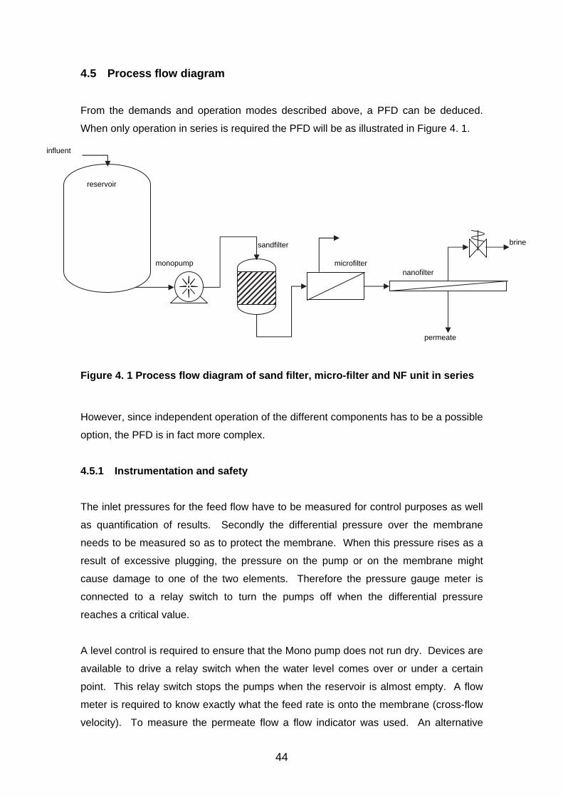
44
4.5 Process flow diagram
From the demands and operation modes described above, a PFD can be deduced.
When only operation in series is required the PFD will be as illustrated in Figure 4. 1.
Figure 4. 1 Process flow diagram of sand filter, micro-filter and NF unit in series
However, since independent operation of the different components has to be a possible
option, the PFD is in fact more complex.
4.5.1 Instrumentation and safety
The inlet pressures for the feed flow have to be measured for control purposes as well
as quantification of results. Secondly the differential pressure over the membrane
needs to be measured so as to protect the membrane. When this pressure rises as a
result of excessive plugging, the pressure on the pump or on the membrane might
cause damage to one of the two elements. Therefore the pressure gauge meter is
connected to a relay switch to turn the pumps off when the differential pressure
reaches a critical value.
A level control is required to ensure that the Mono pump does not run dry. Devices are
available to drive a relay switch when the water level comes over or under a certain
point. This relay switch stops the pumps when the reservoir is almost empty. A flow
meter is required to know exactly what the feed rate is onto the membrane (cross-flow
velocity). To measure the permeate flow a flow indicator was used. An alternative
reservoir
permeate
influent
brine
monopump
sandfilter
microfilter nanofilter

45
measuring technique would be to use a mass balance which can be placed in line with
the help of Sartorius (Sartowedge) software.
With this instrumentation a hybrid diagram of a PFD and a PID is obtained, with
electronic signals shown in dotted lines (Figure 4.2).
Figure 4. 2 Process flow diagram of the NF unit
4.5.2 Bypass
There are three reasons for creating a bypass from the NF module. The first is to be
able to finely adjust the feed flow to the membrane. The Mono pump is indeed
adjustable between several flows, but when one wants to work at a flow that is even
lower than the lowest set flow, or in between two, it would be convenient if one could
bypass some of the feed away from the membrane module. This has to be done
making sure what the exact feed flow is. This is typically a feature that will not appear
in a commercial version of this process.
The second reason for a bypass is for commissioning reasons. When starting up the
plant for the first time, one can expect flow and pressure problems. If this problem
occurs in the pressure-reducing valve, one can blow up the membrane. The third
reason has to do with replacing a membrane. Normally one would have to shut down
MF permeate
Lc
dP
F
F
P
atmospheric
permeate
influent
brine
5
2 bar
1 bar

46
and drain the entire system. Now the system can keep on running. One only has to
release the pressure-reducing valve and drain the part between the two valves where
the membrane is situated.
When doing duration tests, one can choose to lead both permeate and brine/bypass
mixtures back to the reservoir. Then one does not waste all of the bypassed feed while
ensuring constant concentrations. When using only this bypass, one has to ensure
that water is not entering the NF module from the backside. Therefore a valve has to
be added at the brine side of the module.
During operation, one wants to have easy access to all instrumentation and valves. It
is, for example, not favourable to set a valve and have to walk back to see what the
effect on the flow is. Or another example: When pressure rises too quickly, one wants
to be able to switch off the process immediately. Therefore the ambition is to have all
valves and instrumentation in one geometric plane. The best would be to have names
on the equipment as well, so that one can see immediately what is going on.
A final diagram is as in Figure 4. 3 whilst the electrical installations for operating the
pumps are given in Appendix F.
1
MF
Sample
Filter
Borehole water
Dirty Water In
NF feed tank
Drain
Monopump
sample2
sample3
PCV
Control Valve
Sandfilt
PI FIC
FE PID
NF
B1
2
3
Figure 4. 3 Modified NF unit diagram

47
Problems experienced during operation include the danger of the pump running dry
when the unit is not on auto-run. This can occur since the level controllers are not
active as they are not on-line when the manual switch is used. Once dry the pump
burns the rubber at its rotor, which further blocks the pipeline towards the flow
controller. Such blockages cause pressure build-up between the pump and the flow
meter with a risk of damage to the pump. This is to an extent relieved by the pressure
relieve valve which purges excessive pressure and contents back to the reservoir
(green line). Because some membranes have more water and volume flux than the
others the feed flow required at a specific pressure is difficult to attain, especially at
highly permeable membranes. Such membranes have high fluxes and an attempt to
get to higher pressures only cause high permeates of poor quality.
4.6 Testing the unit
4.6.1 Clean water flux
The membranes were tested for clean water flux at 5 bar (Figure 4. 4).
Total volume
Flux(solute)volume/(time.area)
4.03609E-06 4.0360874.1548E-06 4.154796
4.19437E-06 4.1943654.21415E-06 4.214154.22602E-06 4.2260214.23393E-06 4.233935
#DIV/0! #DIV/0!4.22323E-06 4.223228
#DIV/0! #DIV/0! 0.00.51.01.52.02.53.03.54.04.5
0 50 100
Aw (
L.hr
-1.m
-2.b
ar-1
)
Figure 4. 4 Permeabilities of clean water on various membranes
D11 and D12 membranes yielded lower permeabilities (3.05x10⁻⁶ and 3.39x10⁻⁶ L.hr-
1.m-2.bar-1 respectively) compared to the permeabilities attained in the dead-end
module (see Table 3.2). In the dead-end mode, the water permeability in the D11
(9.21x10⁻⁶ L.hr-1.m-2.bar-1) was slightly higher than that of D12 (8.79x10⁻⁶ L.hr-1.m-2.
bar-1). The two values are however, well within the range of those for NF90 and CTC1
(3.10x10⁻⁶ and 4.3x10⁻⁶ L.hr-1.m-2.bar-1, respectively), the values are equivalent to those
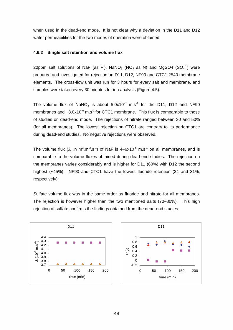
48
when used in the dead-end mode. It is not clear why a deviation in the D11 and D12
water permeabilities for the two modes of operation were obtained.
4.6.2 Single salt retention and volume flux
20ppm salt solutions of NaF (as F-), NaNO3 (NO3 as N) and MgSO4 (SO42-) were
prepared and investigated for rejection on D11, D12, NF90 and CTC1 2540 membrane
elements. The cross-flow unit was run for 3 hours for every salt and membrane, and
samples were taken every 30 minutes for ion analysis (Figure 4.5).
The volume flux of NaNO3 is about 5.0x10⁻⁶ m.s-1 for the D11, D12 and NF90
membranes and ~8.0x10⁻⁶ m.s-1 for CTC1 membrane. This flux is comparable to those
of studies on dead-end mode. The rejections of nitrate ranged between 30 and 50%
(for all membranes). The lowest rejection on CTC1 are contrary to its performance
during dead-end studies. No negative rejections were observed.
The volume flux (Jv in m3.m-2.s-1) of NaF is 4–6x10⁻⁶ m.s-1 on all membranes, and is
comparable to the volume fluxes obtained during dead-end studies. The rejection on
the membranes varies considerably and is higher for D11 (60%) with D12 the second
highest (~45%). NF90 and CTC1 have the lowest fluoride retention (24 and 31%,
respectively).
Sulfate volume flux was in the same order as fluoride and nitrate for all membranes.
The rejection is however higher than the two mentioned salts (70–80%). This high
rejection of sulfate confirms the findings obtained from the dead-end studies.
D11
3.73.83.94.04.14.24.34.4
0 50 100 150 200
time (min)
J v (
10-6
m.s
-1)
D11
-0.20
0.20.40.60.8
1
0 50 100 150 200
time (min)
R (
-)

49
D12
4.6
4.7
4.8
4.9
5.0
5.1
5.2
0 50 100 150 200
time (min)
J v (10
-6 m
.s-1)
D12
0
0.2
0.4
0.6
0.8
1
0 50 100 150 200
time (min)
R (
-)
CTC1
0
2
4
6
8
10
0 50 100 150 200
time (min)
J v (
10-6
m.s
-1)
CTC1
-0.20
0.20.40.60.8
1
0 50 100 150 200
time (min)
R (
-)
NF90
4.2
4.3
4.4
4.5
4.6
4.7
4.8
0 50 100 150 200
time (min)
J v (10
-6 m
.s-1)
NF90
-0.2
0
0.2
0.4
0.6
0.8
1
0 50 100 150 200
time (min)
R (
-)
NaNO3 NaF MgSO4
Figure 4. 5 Volume flux and retention coefficient of various salts on various
membranes
To summarize, the selected membranes show good rejections for divalent sulfate and
poor (up to 50%) for monovalent fluoride and nitrate. This trend is typical of NF
membrane processes in which monovalents are not completely rejected as opposed to
multivalents, which are highly rejected.

50
1. Coulson and Richardson’s Chemical Engineering, volume 6, second edition,
R.K. Sinnott; 1993, Butterworth-Heinemann, Oxford

51
5 Treatment of rural water
The levels of nitrate and fluoride are high in the rural water of some parts of the North
West Province. This water is however ideally suited for this study and was used in an
attempt to remove the nitrate and fluoride concentrations to acceptable or
recommended levels by nanofiltration membrane processes. Other chemical
components including sulfate, chloride, copper, total hardness (TH), and total dissolved
solids (TDS) were also monitored. The sampled water was also classified in terms of
its quality for domestic use with the help of colour coding.
5.1 Pollution and its effect
The management of water use and reuse is made critical by the extensive agricultural
practices (e.g. livestock and crop farming), industrial activities (e.g. gold and platinum
mining), lack of proper sanitation and geohydrochemical influences. The poor quality
of the water available for rural domestic use is of concern. Sadly, however, this
pollution goes unchecked, or is minimally monitored in many towns.
Nitrate, which has harmful biological effects when converted to nitrite, has its many
sources of pollution from human waste (especially due to the use of pit latrines in South
African rural areas), animal waste (due to heavy cattle farming), industrial waste (e.g.
pesticides, food processing, munitions and some polyresin facilities), spills of
nitrogenous compounds, and septic tanks. The most harmful effect of nitrate pollution
is methemoglobinaemia (“blue baby syndrome”) in infants and ruminants. Also, in the
nitrogenous environment and under favourable conditions, algae may grow rapidly if
uncontrolled, with subsequent clogging of valves, pipelines, sprinklers and filtering
equipment, resulting in high maintenance costs.
High fluoride levels are found around Pilanesberg of the North West Province and
around some parts of the Limpopo Province as fluor-deposit in soil and rocks [1, 2].
Fluoride from minerals and in geochemical deposits is released into the subsoil water
sources (aquifers) by the slow natural degradation of fluorine contained in the rocks [3].
Its presence in the groundwater is pH dependent as it only leaches under acidic
conditions. Its harmful effects include skeletal and dental fluorosis characterized by
hardening of skeletal joints and/or mottling (staining) of the teeth.

52
5.2 Experimental
Sampling was done over a two-year period during two different (wet and dry) seasons
(equivalent to a total of 4 sampling opportunities) at numerous locations within the
North West Province (Table 5. 1). Samples were collected in the beginning and middle
of both the dry and wet seasons. The dry season is characterized by high temperature
with very little or no rain, normally at the beginning of spring (from September to
October). As such, not much seepage of pollutants to the groundwater is expected
during this season. Chemical compositions during this season are therefore expected
to be mostly influenced by the rock composition of the aquifers (geohydrochemical
factors). Furthermore, the surface water as well as most of the streams have run dry or
have low water content. As a result, chemical components might concentrate, as the
solute water decreases.
The wet season is characterized by heavy rains (from December to April). During this
period, aquifers are recharged and a lot of chemical seepage can be expected with
subsequent increase in, or dilution (leaching) of, the already present chemical
components. For surface water however, dilution of chemical components is expected.
The areas or locations mentioned in Table 5. 1 were sampled and monitored for nitrate
(NO3-N), fluoride (F-), sulfate (SO42-), chloride (Cl-), total hardness (Ca2+ and Mg2+ as
CaCO3), copper (Cu2+), total dissolved solids (TDS) and pH.
Sampling steps were adapted from the protocols as outlined in the Hach DR/890
manual which adheres to the sampling, storage and analysis specifications according
to the US Environmental Protection Agency. Water quality classification is done in line
with the SA Bureau of Standards (SABS) “Specifications for water for domestic
supplies” (SABS 241, 1998) [4] and the Department of Water Affairs and Forestry’s
“Quality of domestic water supplies ”[5].

53
Table 5. 1 List of locations where water samples were collected
The sampling and storage procedure was as follows:
Clean, acid washed plastic (PTFE) sample holders were used for every sample
(100ml–5000ml);
Before sampling, the stopper and holder were rinsed a number of times with
sample water;
For surface water, the holder was dipped, cautiously not to disturb the bottom
sediments, in the water before it was capped;
Sample name and location
Sample number
Source type Locality description
Kle
rksd
orp
regi
on
Mooi River 1 River River flowing through the sporting fields of the University, from Potch dam.
Potch University 2 Groundwater Borehole within the University terrain, used for irrigation. Boitshoko School
2a Groundwater Borehole in the Ikageng semi-rural area.
Sarafina 2b Groundwater Borehole in the Ikageng rural area, new settlement. Haaskraal 3 Groundwater Cattle and maize farm with about 10 family units. Taaiboschspruit 4 Spring Holiday resort. Dominated by different species of birds. Vaal River 6 River Sampled downstream of the gold mines. Also tourist
destination.
Kos
ter
regi
on
Kaallaagte1 8a Groundwater Domestic use by about 30 family units. Kaallaagte2 8b Groundwater Domestic use by about 30 family units. Rhenosterfontein
9 Groundwater Livestock (cattle) and domestic use by about 6 scattered family units.
Tlholego 1 10a Groundwater Domestic use by about 5 family units. Tlholego 2 10b Groundwater Domestic use by about 5 family units. Tlholego 3 10c Groundwater Domestic use by about 5 family units. Tlholego 4 10d Groundwater Domestic use by about 5 family units. Roodewal 11 Groundwater Livestock (cattle) and domestic use by about 5 scattered
family units.
Rus
tenb
urg
regi
on
Rietvlei 12 Groundwater Around an industrial area. Greenside 13 Groundwater Private borehole, near platinum mines. Mogwase stream
14 Stream Stream normally with drinking cattle on site.
Beestekraal 15 Stream Sampled downstream the dam but closer to the communities.
Bakgatla 20 Groundwater Public tap. Lerome 1 13a Groundwater Public handpump for use by about 100 family units. Lerome 2 21 Groundwater Private borehole. Lerome 3 25 Groundwater Private borehole. Ledig 1 23 Groundwater Public tap. Ledig 2 22 Groundwater Public tap. Lefaragatlhe 24 Groundwater Private tap.
Maf
iken
g
Lichtenburg 5 Groundwater Irrigation water. Lime plant in the vicinity. Mmabatho 16 Groundwater Private borehole. Letlamoreng 1 17 Groundwater Tourist and holiday resort. Cattle and holiday makers
around the dam. Letlamoreng 2 18 Spring Tourist and holiday resort. Cattle and holiday makers
around the dam.

54
For boreholes (mechanical and hand pumps), the pump was operated for some
time with subsequent bottle rinsing before sampling;
Samples from running streams were taken as close as possible to the middle of the
stream (crocodiles were friendly!);
Electrical conductivity and pH were measured on site.
A wide distribution of sampling was necessary to elucidate the water quality status in
the Province. Both the south-east and the north-west of the Province were not
sampled due to travelling constraints. The sample points were grouped into four
regions (Klerksdorp, Rustenburg, Koster and Mafikeng Regions). Groundwater was
the main sampling target although streams, rivers and catchments (or springs) were
also sampled.
The following instruments were used for the sample analysis:
An ion chromatograph (IC) with Waters column IC-Pak anion HC, Model 430
conductivity detector and Model510 pump for the analysis of NO3-, Cl- and
SO42-;
An atomic absorption analyser (AA Varian 250+) was used for the analysis of Ca2+
and Mg2+;
A colorimeter of Hach DR/890 was used for the analysis of NO3-N, F-, Cl-, SO42-
and total hardness (as CaCO3);
A pH301 from Hanna Instruments was used for pH detection and
A Hanna Instruments’ HI 9032 conductimeter was used for the conductometric (and
TDS) determination.
The complete sampling data is shown in Appendix G, including tables of average and
maximum chemical components (Appendices H and I). A combined graphical
presentation is shown in Appendix J.
5.3 Water classification methodology
The sampled water was classified specifically for domestic use in terms of drinking
(health and aesthetic), food preparation, bathing and laundry for every concentration of
pollutant analysed. In Table 5. 2 the structure of the classification system with
description of the effects of different classes of water on various domestic uses is
shown. Such an approach gives an idea of how suitable water is for these various
domestic uses.
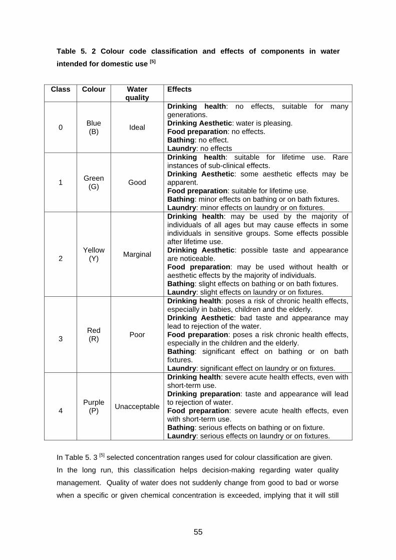
55
Table 5. 2 Colour code classification and effects of components in water
intended for domestic use [5]
In Table 5. 3 [5] selected concentration ranges used for colour classification are given.
In the long run, this classification helps decision-making regarding water quality
management. Quality of water does not suddenly change from good to bad or worse
when a specific or given chemical concentration is exceeded, implying that it will still
Class Colour Water quality
Effects
0 Blue (B)
Ideal
Drinking health: no effects, suitable for many generations. Drinking Aesthetic: water is pleasing. Food preparation: no effects. Bathing: no effect. Laundry: no effects
1 Green
(G) Good
Drinking health: suitable for lifetime use. Rare instances of sub-clinical effects. Drinking Aesthetic: some aesthetic effects may be apparent. Food preparation: suitable for lifetime use. Bathing: minor effects on bathing or on bath fixtures. Laundry: minor effects on laundry or on fixtures.
2
Yellow (Y)
Marginal
Drinking health: may be used by the majority of individuals of all ages but may cause effects in some individuals in sensitive groups. Some effects possible after lifetime use. Drinking Aesthetic: possible taste and appearance are noticeable. Food preparation: may be used without health or aesthetic effects by the majority of individuals. Bathing: slight effects on bathing or on bath fixtures. Laundry: slight effects on laundry or on fixtures.
3
Red (R)
Poor
Drinking health: poses a risk of chronic health effects, especially in babies, children and the elderly. Drinking Aesthetic: bad taste and appearance may lead to rejection of the water. Food preparation: poses a risk chronic health effects, especially in the children and the elderly. Bathing: significant effect on bathing or on bath fixtures. Laundry: significant effect on laundry or on fixtures.
4
Purple (P)
Unacceptable
Drinking health: severe acute health effects, even with short-term use. Drinking preparation: taste and appearance will lead to rejection of water. Food preparation: severe acute health effects, even with short-term use. Bathing: serious effects on bathing or on fixture. Laundry: serious effects on laundry or on fixtures.

56
be usable for some time before it will have unbearable effects. Classification is done
by use of a colour coding range from ideal to totally unacceptable water quality.
Table 5. 3 Concentration ranges of various chemical components used in water
colour classification
Range <450 450–1000 1000–2400
2400–3400
> 3400 -
Tot
al
diss
olve
d so
lids
(mg.
L-1)
Drinking (H) B G Y R P - Drinking (A) B G Y R P -
Food preparation
B G Y R P -
Bathing B B B G Y - Laundry B B G Y R -
Range < 0.7 0.7 – 1.0 1.0 – 1.5 1.5 – 3.5 > 3.5
Flu
orid
e (m
g.L-1
)
Drinking (H) B G Y R P - Drinking (A) B B B B B -
Food preparation
B G Y R P -
Bathing B B B B B - Laundry B B B B B -
Range < 6 6 – 10 10 – 20 20 – 40 > 40 -
Nitr
ate
(mg.
L-1 a
s ni
trog
en)
Drinking (H) B G B R P - Drinking (A) B B B B B -
Food preparation
B G B R P -
Bathing B B G Y R - Laundry B B B B B -
Range <100 100 – 200 200 – 400 400 – 600
600 – 1000
> 1000
Sul
fate
(m
g.L-1
)
Drinking (H) B B G Y R P Drinking (A) B B G Y R P
Food preparation
B B G Y R P
Bathing B B B G Y R Laundry B B G Y R P
Range < 100 100 – 200 200 – 600
600 - 1200
> 1200 -
Chl
orid
e (m
g.L-1
)
Drinking (H) B G Y R P - Drinking (A) B G Y R P -
Food preparation
B G Y R P -
Bathing B B B B B - Laundry B G Y R P -
H = health, A = aesthetic. B = blue (ideal), G = green (good), Y = yellow (marginal), R = red
(poor), P = purple (completely unacceptable)

57
5.4 Water sampling and monitoring
Samples were collected during the beginning and middle of the dry and wet seasons to
cover the full range of possible conditions. The samples collected during the wet
season (middle rainy season (MRS) and beginning rainy season (BRS)) indicate that
the chemical components (pollutants) were well below their recommended limits
(Figure 5. 1). This means that both the groundwater and surface water components
are diluted by continued water recharge resulting in improved ground water quality.
Middle of rainy season
0
2
4
6
8
10
12
14
16
1 2 2a 2b 3 4 6 8a 8b 910
a10
b10
c10
d 11 12 13 14 15 20 13a 21 25 23 22 24 5 16 17 18
conc
entr
atio
n (p
pm)
fluoride (ppm) nitrate as N (ppm)
A B C D
Begin of rainy season
02468
10121416
1 2 2a 2b 3 4 6 8a 8b 910
a10
b10
c10
d 11 12 13 14 15 20 13a 21 25 23 22 24 5 16 17 18
conc
entr
atio
n (p
pm)
fluoride (ppm) nitrate as N (ppm)
A B C D
Figure 5. 1 Selected chemical component concentrations recorded for various
sampling sites during the wet season (A = Klerksdorp, B = Koster, C =
Rustenburg, and D = Mafikeng Regions. x-axis = sampling points)

58
When sampled immediately after the first rainfall (BRS), increased concentrations of
chemical components are observed although not as high as those observed during the
dry seasons (beginning dry season (BDS) and middle dry season (MDS)) as presented
in Figure 5. 2.
Middle dry season
0
2
4
6
8
10
12
14
1 2
2a 2b
3 4 6
8a 8b
9
10a
10b
10c
10d 11 12 13 14 15 20
13a 21 25 23 22 24
5
16 17 18
con
cen
trat
ion
(p
pm
)
fluoride nitrate as N
A B C D
Begin of dry season
0
2
4
6
8
10
12
14
16
1
2a
3 6
8b
10a
10c
11 13 15
13a 25 22
5
17
conc
entr
atio
n (p
pm)
fluoride (ppm) nitrate as N (ppm)
A B C D
Figure 5. 2 Selected chemical component concentrations recorded for various
sampling sites during dry seasons (A = Klerksdorp, B = Koster, C = Rustenburg,
and D = Mafikeng Regions. x-axis = sampling points)

59
The nitrate concentration is low in groundwater (sample points 2, 5, 9–13, 16, 18–25)
during the dry season but increases immediately after the first rains. This is probably
due to seepage/leaching of nitrate that was adsorbed by the soil. Also, during dry
seasons, farming activities are low and any nitrate pollutants (and other ions) are held
in the soil. These nitrates will enter the aquifers during the first rain, leading to an
increase in concentrations (Figure 5. 2).
Sulfate concentrations (see Appendix G – J) seemed to be low during wet seasons
but slightly higher during dry seasons, increasing further immediately after the first
rainfalls as it is leached from the soil into the aquifers. Fluoride is within acceptable
limits within all regions except the Rustenburg region (marked C) where it is at
unacceptable levels throughout the year.
Figure 5. 3 shows the graphical presentation of the average concentration of chemical
components (for four sampling opportunities) in surface (sample points 1, 3, 4, 6, 14,
15 and 17) and groundwater (2, 5, 9–13, 16, 18–25).
0
2
4
6
8
10
12
14
16
1 2 2a 2b 3 4 6 8a 8b 910
a10
b10
c10
d 11 12 13 14 15 20 13a 21 25 23 22 24 5 16 17 18
conc
netr
atio
n (
ppm
)
fluoride (ppm) nitrate as N (ppm)
A B C D
Figure 5. 3 Average chemical component concentrations recorded for various
sampling sites over one year (A = Klerksdorp, B = Koster sub-, C = Rustenburg,
and D = Mafikeng Regions. x-axis = sampling points)
Due to the nitrate (as nitrogen) concentration found in the private borehole (sample 13)
within the Rustenburg region, the water is of marginal quality (Figure 5. 3), which gives
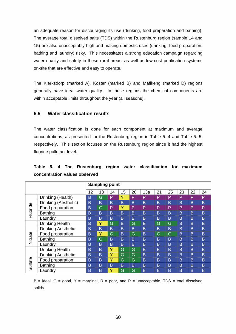
60
an adequate reason for discouraging its use (drinking, food preparation and bathing).
The average total dissolved salts (TDS) within the Rustenburg region (sample 14 and
15) are also unacceptably high and making domestic uses (drinking, food preparation,
bathing and laundry) risky. This necessitates a strong education campaign regarding
water quality and safety in these rural areas, as well as low-cost purification systems
on-site that are effective and easy to operate.
The Klerksdorp (marked A), Koster (marked B) and Mafikeng (marked D) regions
generally have ideal water quality. In these regions the chemical components are
within acceptable limits throughout the year (all seasons).
5.5 Water classification results
The water classification is done for each component at maximum and average
concentrations, as presented for the Rustenburg region in Table 5. 4 and Table 5. 5,
respectively. This section focuses on the Rustenburg region since it had the highest
fluoride pollutant level.
Table 5. 4 The Rustenburg region water classification for maximum
concentration values observed
Sampling point
12 13 14 15 20 13a 21 25 23 22 24
Flu
orid
e
Drinking (Health) B G P Y P P P P P P P Drinking (Aesthetic) B B B B B B B B B B B Food preparation B G P Y P P P P P P P Bathing B B B B B B B B B B B Laundry B B B B B B B B B B B
Nitr
ate
Drinking Health B Y G B G B G G B B B Drinking Aesthetic B B B B B B B B B B B Food preparation B Y G B G B G G B B B Bathing B G B B B B B B B B B Laundry B B B B B B B B B B B
Sul
fate
Drinking Health B B Y G G B B B B B B Drinking Aesthetic B B Y G G B B B B B B Food preparation B B Y G G B B B B B B Bathing B B B B B B B B B B B Laundry B B Y G G B B B B B B
B = ideal, G = good, Y = marginal, R = poor, and P = unacceptable. TDS = total dissolved
solids.
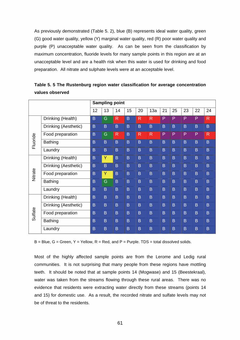
61
As previously demonstrated (Table 5. 2), blue (B) represents ideal water quality, green
(G) good water quality, yellow (Y) marginal water quality, red (R) poor water quality and
purple (P) unacceptable water quality. As can be seen from the classification by
maximum concentration, fluoride levels for many sample points in this region are at an
unacceptable level and are a health risk when this water is used for drinking and food
preparation. All nitrate and sulphate levels were at an acceptable level.
Table 5. 5 The Rustenburg region water classification for average concentration
values observed
Sampling point
12 13 14 15 20 13a 21 25 23 22 24
Flu
orid
e
Drinking (Health) B G R B R R P P P P R
Drinking (Aesthetic) B B B B B B B B B B B
Food preparation B G R B R R P P P P R
Bathing B B B B B B B B B B B
Laundry B B B B B B B B B B B
Nitr
ate
Drinking (Health) B Y B B B B B B B B B
Drinking (Aesthetic) B B B B B B B B B B B
Food preparation B Y B B B B B B B B B
Bathing B G B B B B B B B B B
Laundry B B B B B B B B B B B
Sul
fate
Drinking (Health) B B B B B B B B B B B
Drinking (Aesthetic) B B B B B B B B B B B
Food preparation B B B B B B B B B B B
Bathing B B B B B B B B B B B
Laundry B B B B B B B B B B B
B = Blue, G = Green, Y = Yellow, R = Red, and P = Purple. TDS = total dissolved solids.
Most of the highly affected sample points are from the Lerome and Ledig rural
communities. It is not surprising that many people from these regions have mottling
teeth. It should be noted that at sample points 14 (Mogwase) and 15 (Beestekraal),
water was taken from the streams flowing through these rural areas. There was no
evidence that residents were extracting water directly from these streams (points 14
and 15) for domestic use. As a result, the recorded nitrate and sulfate levels may not
be of threat to the residents.
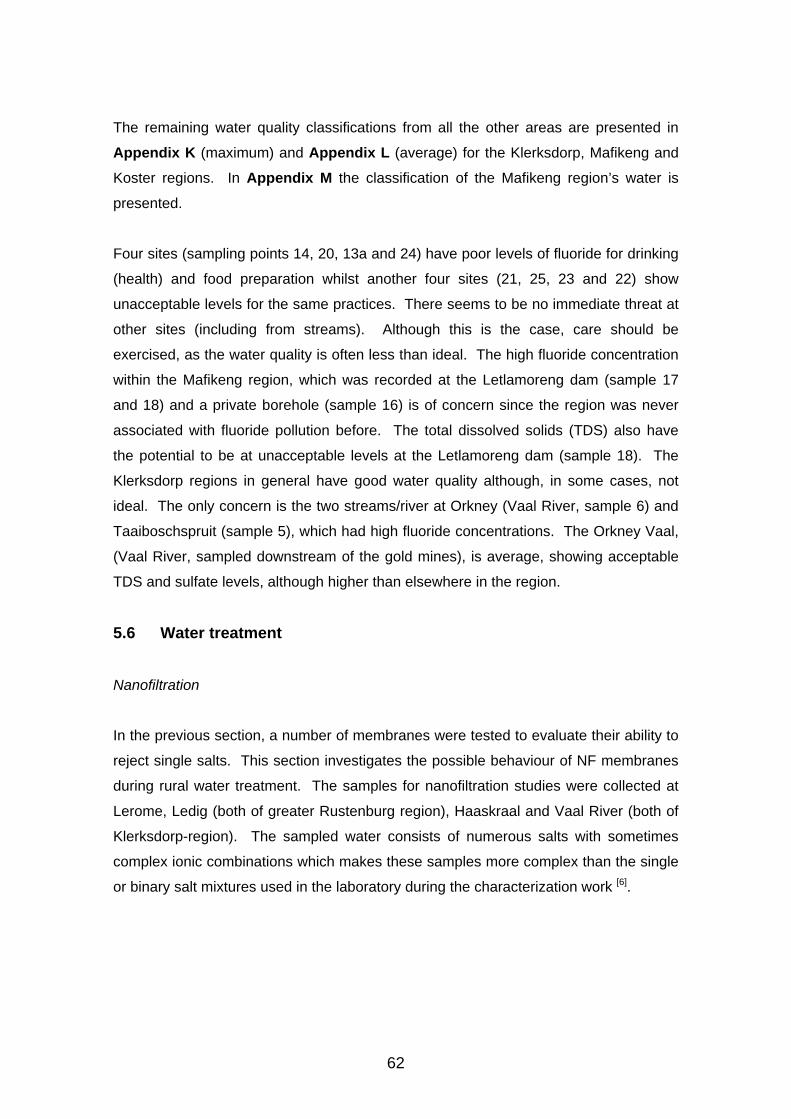
62
The remaining water quality classifications from all the other areas are presented in
Appendix K (maximum) and Appendix L (average) for the Klerksdorp, Mafikeng and
Koster regions. In Appendix M the classification of the Mafikeng region’s water is
presented.
Four sites (sampling points 14, 20, 13a and 24) have poor levels of fluoride for drinking
(health) and food preparation whilst another four sites (21, 25, 23 and 22) show
unacceptable levels for the same practices. There seems to be no immediate threat at
other sites (including from streams). Although this is the case, care should be
exercised, as the water quality is often less than ideal. The high fluoride concentration
within the Mafikeng region, which was recorded at the Letlamoreng dam (sample 17
and 18) and a private borehole (sample 16) is of concern since the region was never
associated with fluoride pollution before. The total dissolved solids (TDS) also have
the potential to be at unacceptable levels at the Letlamoreng dam (sample 18). The
Klerksdorp regions in general have good water quality although, in some cases, not
ideal. The only concern is the two streams/river at Orkney (Vaal River, sample 6) and
Taaiboschspruit (sample 5), which had high fluoride concentrations. The Orkney Vaal,
(Vaal River, sampled downstream of the gold mines), is average, showing acceptable
TDS and sulfate levels, although higher than elsewhere in the region.
5.6 Water treatment
Nanofiltration
In the previous section, a number of membranes were tested to evaluate their ability to
reject single salts. This section investigates the possible behaviour of NF membranes
during rural water treatment. The samples for nanofiltration studies were collected at
Lerome, Ledig (both of greater Rustenburg region), Haaskraal and Vaal River (both of
Klerksdorp-region). The sampled water consists of numerous salts with sometimes
complex ionic combinations which makes these samples more complex than the single
or binary salt mixtures used in the laboratory during the characterization work [6].

63
5.7 Dead-end studies
The water samples were nanofiltered through the NF membranes at a trans-membrane
pressure difference of 20bar without any pre-treatment. The concentration of each
component (pollutant) in every sample was monitored for feed, permeate and brine
chemical composition with subsequent calculation of the retention coefficient using
Equation 5.1:
f
p
C
CR 1 100% (5. 1)
where Cp and Cf are the permeate and feed concentrations (in ppm), respectively.
The unit was stirred at the maximum possible speed to minimize concentration
polarization and to hinder possible fouling. The pH of the samples was not adjusted
and the experiments were carried out at ambient temperatures. Ion chromatography,
atomic adsorption, conductimeter and a colorimeter were used for concentration
monitoring.
Selected rural groundwater sites (sample 13a, 22, 3) and the stream water of the Vaal
River (sample site 6) were chosen for treatment by nanofiltration. Site 3 was chosen
because it is in a farming area (cattle and maize farm), is in the proximity of the
Potchefstroom University and showed high nitrate levels. Sites 22 and 13a were
chosen because they are in the rural Rustenburg area and have higher levels of
fluoride and nitrate than any other sampled area. Site 6 was chosen because the
sampling point in the Vaal River is downstream from the gold mines, and has low
nitrate and fluoride levels but high sulfate levels.
In the following sections, results of the treatments of the various water samples are
presented.
5.7.1 Lerome (sample 13a)
According to Figure 5. 4, improvement of the Lerome rural water was achieved with all
the tested membranes (D11, D12, NF90, NF70, TFC-S, TFC-SR, TFC-ULP and
CTC1). Sulfate was retained (up to 100%) by the membranes (Figure 5. 4) confirming

64
that the membranes are negatively charged as characterized [6]. Total hardness (TH) is
poorly rejected by D11 and CTC1 (about 20%) and well rejected by all other
membranes. Total dissolved solids (TDS) is moderately rejected by all membranes
(30–60%).
Monovalents (fluoride and nitrate) showed negative rejection on some membranes.
These monovalent co-ions are transported through the membrane in the presence of
high valence co-ions. Such negative rejections are due to increased transport induced
by the high valence co-ions, causing the permeate concentration to be higher than the
feed concentration. For the Lerome rural water (containing high levels of fluoride)
negative fluoride rejection is, in particular, observed for the TFC-SR and D12
membranes whilst D11, NF90 and CTC-1 show poor rejections (5–20%). Good
fluoride retentions are recorded only for the membranes TFC-S (~70%), and NF70
(~75%).
Lerome
-0.2
0
0.2
0.4
0.6
0.8
1
1.2
TFC-S TFC-ULP D11 D12 NF70 NF90 TFC-SR CTC-1
R (
-)
fluoride nitrate sulfate TH TDS
Figure 5. 4 Retention coefficient of various NF membranes on the treatment of
the Lerome groundwater (Pressure = 20 bar, temperature = 20oC. x-axis =
membrane types)
Nitrate is negatively rejected by TFC-SR and D12 and poorly rejected by D11, NF90
and CTC1 (1–20%). Good nitrate rejection is again observed on TFC-S (~70%), NF70
(~75%) and also TFC-ULP (~90%). Figure 5. 5 summarizes rejections for different ions
and membranes used in the Lerome water treatment.

65
Lerome
-0.2
0
0.2
0.4
0.6
0.8
1
1.2
fluoride nitrate sulfate TH TDS
R (
-)
TFC-S TFC-ULP D11 D12 NF70 NF90 TFC-SR CTC-1
Figure 5. 5 Presentation of membrane performance for Lerome groundwater
(Pressure = 20 bar, temperature = ambient)
5.7.2 Ledig (sample 23)
The efficiency of the removal of ions from the Ledig (a rural area in Rustenburg) water
sample differed for varying membranes (Figure 5. 6). Sulfate rejection is excellent
(>95%) whilst TH is well reduced by all membranes (60–80%) except for TFC-S and
TFC-ULP. TDS is moderately rejected by all membranes (30–60%). This is
comparable to the performance of these membranes for the Lerome water.
Good rejection of nitrate is attained for the Ledig rural water on TFC-S (~58%), NF90
(~70%) and NF70 (~80%) (Figure 5. 6). TFC-ULP also performed poorly, even though
it showed better rejections of this anion on the Lerome rural water owing to the effect
of different other ions (e.g. chloride, copper, sulfate, magnesium, etc.) in the different
water sources. Fluoride levels detected in the Ledig water are as high as in the
Lerome water. The rejection is negative for the NF90 and D11 (was positive for the
Lerome water treatment on both membranes). Moderate fluoride rejection is attained
by all other membranes (10–30%). TFC-S retains fluoride in the Ledig poorly (~15%)
compared to 70% fluoride rejection observed for the Lerome water.
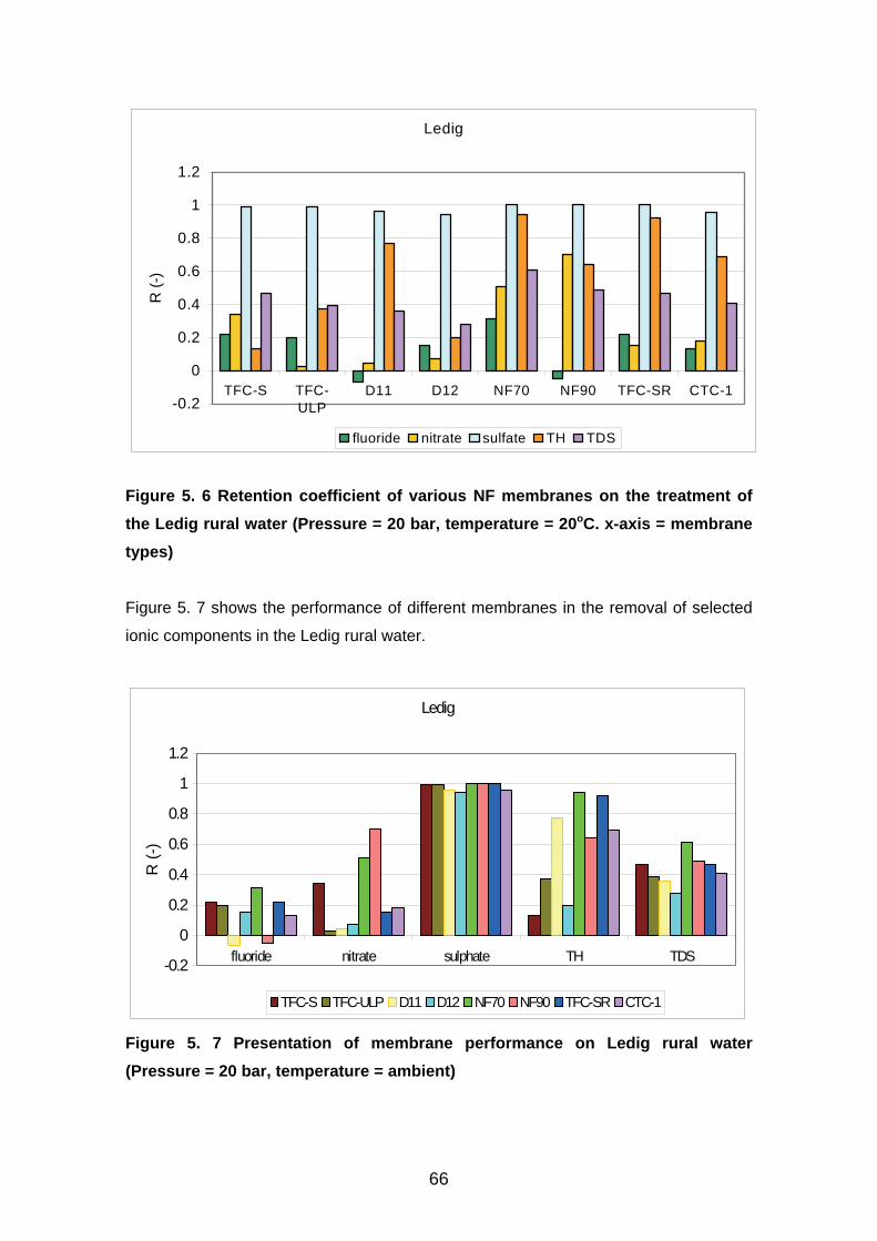
66
Ledig
-0.2
0
0.2
0.4
0.6
0.8
1
1.2
TFC-S TFC-ULP
D11 D12 NF70 NF90 TFC-SR CTC-1
R (
-)
fluoride nitrate sulfate TH TDS
Figure 5. 6 Retention coefficient of various NF membranes on the treatment of
the Ledig rural water (Pressure = 20 bar, temperature = 20oC. x-axis = membrane
types)
Figure 5. 7 shows the performance of different membranes in the removal of selected
ionic components in the Ledig rural water.
Ledig
-0.2
0
0.2
0.4
0.6
0.8
1
1.2
fluoride nitrate sulphate TH TDS
R (
-)
TFC-S TFC-ULP D11 D12 NF70 NF90 TFC-SR CTC-1
Figure 5. 7 Presentation of membrane performance on Ledig rural water
(Pressure = 20 bar, temperature = ambient)

67
5.7.3 Haaskraal (sample 3)
Similarly, sulfate removal was excellent in the Haaskraal (cattle and maize farm) water
sample (Figure 5. 8). This rejection, although not as high as in the Lerome and Ledig
rural water, ranged from 90–100%. The sulfate content in this water was higher than
that of Lerome and Ledig. It is not clear what causes this slight decreased rejection of
sulfate. Again, the rejection of TH is high for the TFC-SR (~90%), NF70 (~85%), NF90
(~70%) and D11 (~78%) membranes. Moderate TH rejection were shown by TFC-ULP
(~38%) whilst TFC-S (~9%) and D12 (~30%) showed poor rejections. TDS, like in
Lerome and Ledig, is moderately rejected by all membranes.
Only TFC-ULP showed negative rejection for nitrate whilst, contrary to Lerome and
Ledig, TFC-S showed improved nitrate rejection (~55%). D11, D12, TFC-SR and
CTC1 all show poor to moderate nitrate rejection (1–30%). Good nitrate rejection is
recorded for the NF70 and NF90 membranes (70–80%). Negative fluoride rejections
are noticed for CTC-1 and NF90 membranes. TFC-S, D12, NF70 and TFC-SR
rejected fluoride poorly (10–30%). Good fluoride rejection is observed for the TFC-ULP
and D11 (60–70%) membranes.
Haaskraal
-0.2
0
0.2
0.4
0.6
0.8
1
1.2
TFC-S TFC-ULP
D11 D12 NF70 NF90 TFC-SR CTC-1
R (
-)
fluoride nitrate sulfate TH TDS
Figure 5. 8 Retention coefficient of various NF membranes on the treatment of
the Haaskraal water components (Pressure = 20 bar, temperature = 20oC. x-axis =
membrane type)
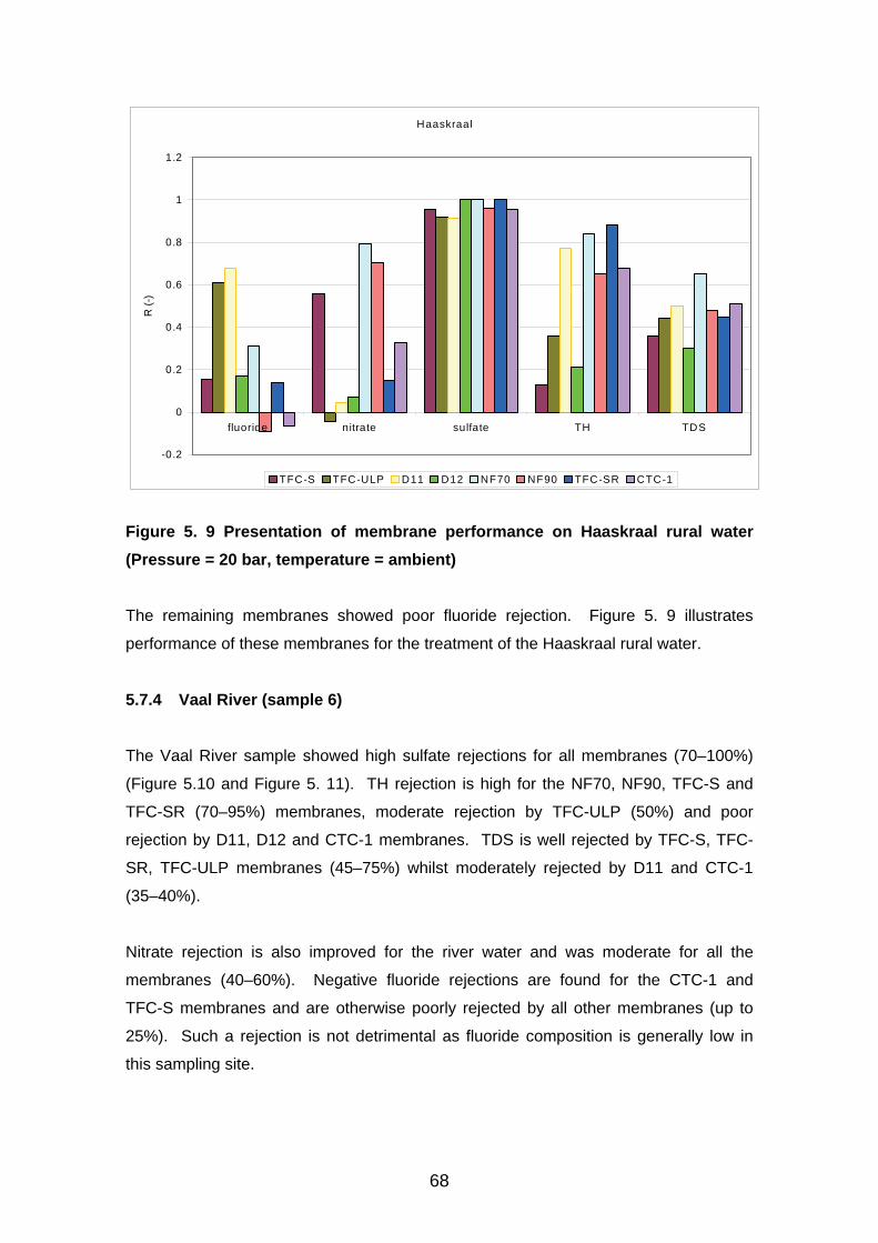
68
Haaskraal
-0.2
0
0.2
0.4
0.6
0.8
1
1.2
fluoride nitrate sulfate TH TDS
R (
-)
TFC-S TFC-ULP D11 D12 NF70 NF90 TFC-SR CTC-1
Figure 5. 9 Presentation of membrane performance on Haaskraal rural water
(Pressure = 20 bar, temperature = ambient)
The remaining membranes showed poor fluoride rejection. Figure 5. 9 illustrates
performance of these membranes for the treatment of the Haaskraal rural water.
5.7.4 Vaal River (sample 6)
The Vaal River sample showed high sulfate rejections for all membranes (70–100%)
(Figure 5.10 and Figure 5. 11). TH rejection is high for the NF70, NF90, TFC-S and
TFC-SR (70–95%) membranes, moderate rejection by TFC-ULP (50%) and poor
rejection by D11, D12 and CTC-1 membranes. TDS is well rejected by TFC-S, TFC-
SR, TFC-ULP membranes (45–75%) whilst moderately rejected by D11 and CTC-1
(35–40%).
Nitrate rejection is also improved for the river water and was moderate for all the
membranes (40–60%). Negative fluoride rejections are found for the CTC-1 and
TFC-S membranes and are otherwise poorly rejected by all other membranes (up to
25%). Such a rejection is not detrimental as fluoride composition is generally low in
this sampling site.
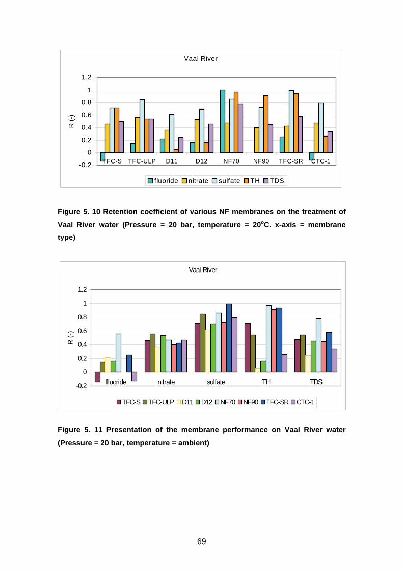
69
Vaal River
-0.2
0
0.2
0.4
0.6
0.8
1
1.2
TFC-S TFC-ULP D11 D12 NF70 NF90 TFC-SR CTC-1
R (
-)
f luoride nitrate sulfate TH TDS
Figure 5. 10 Retention coefficient of various NF membranes on the treatment of
Vaal River water (Pressure = 20 bar, temperature = 20oC. x-axis = membrane
type)
Vaal River
-0.2
0
0.2
0.4
0.6
0.8
1
1.2
fluoride nitrate sulfate TH TDS
R (
-)
TFC-S TFC-ULP D11 D12 NF70 NF90 TFC-SR CTC-1
Figure 5. 11 Presentation of the membrane performance on Vaal River water
(Pressure = 20 bar, temperature = ambient)

70
5.7.5 Fluoride rejection
Fluoride levels are a cause for concern due to high levels in the North West Province.
Successfully removing or reducing it to acceptable levels from the affected water will
bring hope of improving water quality in the rural areas. This section compares
performance of various membranes (TFC-S, TFC-ULP, D11, D12, NF70, NF90, TFC-
SR and CTC1) in reducing fluoride from water samples (Lerome, Ledig, Haaskraal, and
Vaal River) of different initial fluoride levels. Furthermore, the overall performance of
these membranes in improving water fluoride content are compared to each other.
5.7.6 Effect of initial fluoride concentration
The effect of initial fluoride concentration of sampled water on rejection is shown in
Table 5. 6. TFC-S, TFC-ULP and NF70 membranes had high rejections for high
fluoride levels (Lerome). NF90, TFC-SR and CTC1 membranes had poor rejections.
Poor rejections for both high and low levels of fluoride were observed at all sampling
sites when TFC-SR, CTC1, NF90 and D12 membranes are used. D11 had poor
rejection for all the sampled water except for the Haaskraal water (70%) which is
already low in fluoride.
In general, high rejections are observed for higher fluoride concentrations. The
rejections at Vaal River are influenced by a high sulfate content leading to zero or
negative rejections (by “pushing” the monovalents through the membrane). This is
consistent with the observed trend when divalent co-ion levels are high [6]. The NF70
membrane rejects the fluoride even in the presence of high sulfate level, suggesting
that the membrane has more reverse osmosis properties than other nanofiltration
membranes. This RO property of NF70 confirms earlier observations made in our
laboratory[6].
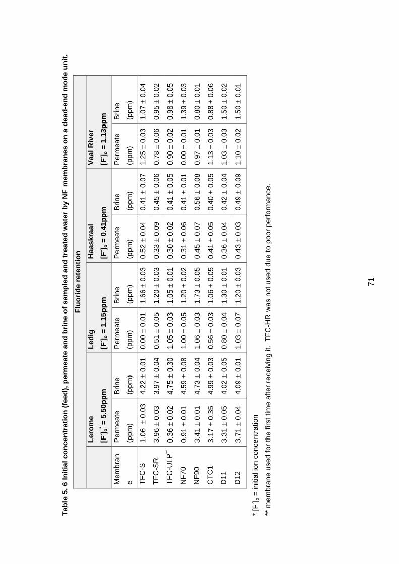
71
Tab
le 5
. 6 In
itia
l co
nce
ntr
atio
n (
feed
), p
erm
eate
an
d b
rin
e o
f sa
mp
led
an
d t
reat
ed w
ater
by
NF
mem
bra
nes
on
a d
ead
-en
d m
od
e u
nit
.
Flu
ori
de
rete
nti
on
L
ero
me
[F- ] o
* = 5
.50p
pm
Led
ig
[F- ] o
= 1
.15p
pm
Haa
skra
al
[F- ] o
= 0
.41p
pm
Vaa
l Riv
er
[F- ] o
= 1
.13p
pm
Mem
bran
e
Per
mea
te
(ppm
)
Brin
e
(ppm
)
Per
mea
te
(ppm
)
Brin
e
(ppm
)
Per
mea
te
(ppm
)
Brin
e
(ppm
)
Per
mea
te
(ppm
)
Brin
e
(ppm
)
TF
C-S
1.
06
0.0
3 4.
22
0.0
1 0.
00
0.0
1 1.
66
0.0
3 0.
52
0.0
4 0.
41
0.0
7 1.
25
0.0
3 1.
07
0.0
4
TF
C-S
R
3.96
0
.03
3.97
0
.04
0.51
0
.05
1.20
0
.03
0.33
0
.09
0.45
0
.06
0.78
0
.06
0.95
0
.02
TF
C-U
LP**
0.36
0
.02
4.75
0
.30
1.05
0
.03
1.05
0
.01
0.30
0
.02
0.41
0
.05
0.90
0
.02
0.98
0
.05
NF
70
0.91
0
.01
4.59
0
.08
1.00
0
.05
1.20
0
.02
0.31
0
.06
0.41
0
.01
0.00
0
.01
1.39
0
.03
NF
90
3.41
0
.01
4.73
0
.04
1.06
0
.03
1.73
0
.05
0.45
0
.07
0.56
0
.08
0.97
0
.01
0.80
0
.01
CT
C1
3.
17
0.3
5 4.
99
0.0
3 0.
56
0.0
3 1.
06
0.0
5 0.
41
0.0
5 0.
40
0.0
5 1.
13
0.0
3 0.
88
0.0
6
D11
3.
31
0.0
5 4.
02
0.0
5 0.
80
0.0
4 1.
30
0.0
1 0.
36
0.0
4 0.
42
0.0
4 1.
03
0.0
3 1.
50
0.0
2
D12
3.
71
0.0
4 4.
09
0.0
1 1.
03
0.0
7 1.
20
0.0
3 0.
43
0.0
3 0.
49
0.0
9 1.
10
0.0
2 1.
50
0.0
1
* [F
- ] o =
initi
al io
n co
ncen
trat
ion
** m
em
bran
e us
ed fo
r th
e fir
st ti
me
afte
r re
ceiv
ing
it. T
FC
-HR
was
not
use
d du
e to
poo
r pe
rfor
man
ce.

72
5.8 Cross-flow studies
5.8.1 Sampled water characteristics
The chemical composition of the sampled water for the cross-flow studies presented
in Table 5. 7 correlates with the composition found previously (see Figure 5. 1 to
Figure 5. 3). The samples were nanofiltered on various membranes (D11, D12,
CTC1 and NF90) at 5bar for about 30 hours using the cross-flow unit discussed in
the previous section. The choice of the membranes was based on their availability
and performance on dead-end modules when using single salts. The reasons for
choosing the selected sites remain the same as discussed for the dead-end mode
studies.
Table 5. 7 Sampled water chemical composition and characteristics
NO3-N Na+ F- TH Cl- SO42- Cu2+ TDS pH
Lerome 1.2 80 5.8 51 36 50 0.01 900 7.0
Ledig 1.8 113 6.9 19 40 22 0.13 832 6.6
Haaskraal 13.9 60 0.2 32 29 70 0.04 1000 7.3
Vaal River 1.6 210 2.7 18 41 112 0.02 1108 6.8
5.8.2 Lerome (sample 13a)
The sulfate and TDS levels are well rejected by all membranes tested (Figure 5. 12 –
see also Appendix O). Water is softened well by all the membranes except CTC1.
This poor performance of CTC1 is consistent with earlier investigations on dead-end
mode. The monovalent ions (nitrate and fluoride) are not well rejected. Nitrate is
poorly rejected by all membranes (8-20%) except for NF90, which rejected fluoride in
the Lerome water by up to 70%. This rejection behaviour is not in line with the
observations made during dead-end studies in which nitrate was rejected by all
membranes. Fluoride is poorly rejected by all membranes. No negative rejections
were observed for all membranes as observed in earlier studies.
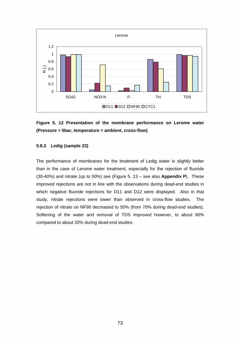
73
Lerome
0
0.2
0.4
0.6
0.8
1
1.2
SO42- NO3-N F- TH TDS
R (
-)
D11 D12 NF90 CTC1
Figure 5. 12 Presentation of the membrane performance on Lerome water
(Pressure = 5bar, temperature = ambient, cross-flow)
5.8.3 Ledig (sample 23)
The performance of membranes for the treatment of Ledig water is slightly better
than in the case of Lerome water treatment, especially for the rejection of fluoride
(30-40%) and nitrate (up to 50%) see (Figure 5. 13 – see also Appendix P). These
improved rejections are not in line with the observations during dead-end studies in
which negative fluoride rejections for D11 and D12 were displayed. Also in that
study, nitrate rejections were lower than observed in cross-flow studies. The
rejection of nitrate on NF90 decreased to 50% (from 70% during dead-end studies).
Softening of the water and removal of TDS improved however, to about 90%
compared to about 20% during dead-end studies.
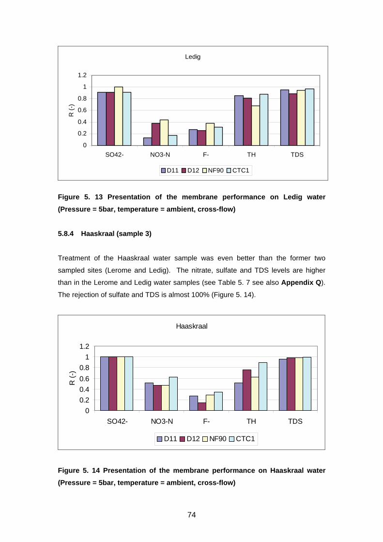
74
Ledig
0
0.2
0.4
0.6
0.8
1
1.2
SO42- NO3-N F- TH TDS
R (
-)
D11 D12 NF90 CTC1
Figure 5. 13 Presentation of the membrane performance on Ledig water
(Pressure = 5bar, temperature = ambient, cross-flow)
5.8.4 Haaskraal (sample 3)
Treatment of the Haaskraal water sample was even better than the former two
sampled sites (Lerome and Ledig). The nitrate, sulfate and TDS levels are higher
than in the Lerome and Ledig water samples (see Table 5. 7 see also Appendix Q).
The rejection of sulfate and TDS is almost 100% (Figure 5. 14).
Haaskraal
0
0.2
0.4
0.6
0.8
1
1.2
SO42- NO3-N F- TH TDS
R (
-)
D11 D12 NF90 CTC1
Figure 5. 14 Presentation of the membrane performance on Haaskraal water
(Pressure = 5bar, temperature = ambient, cross-flow)
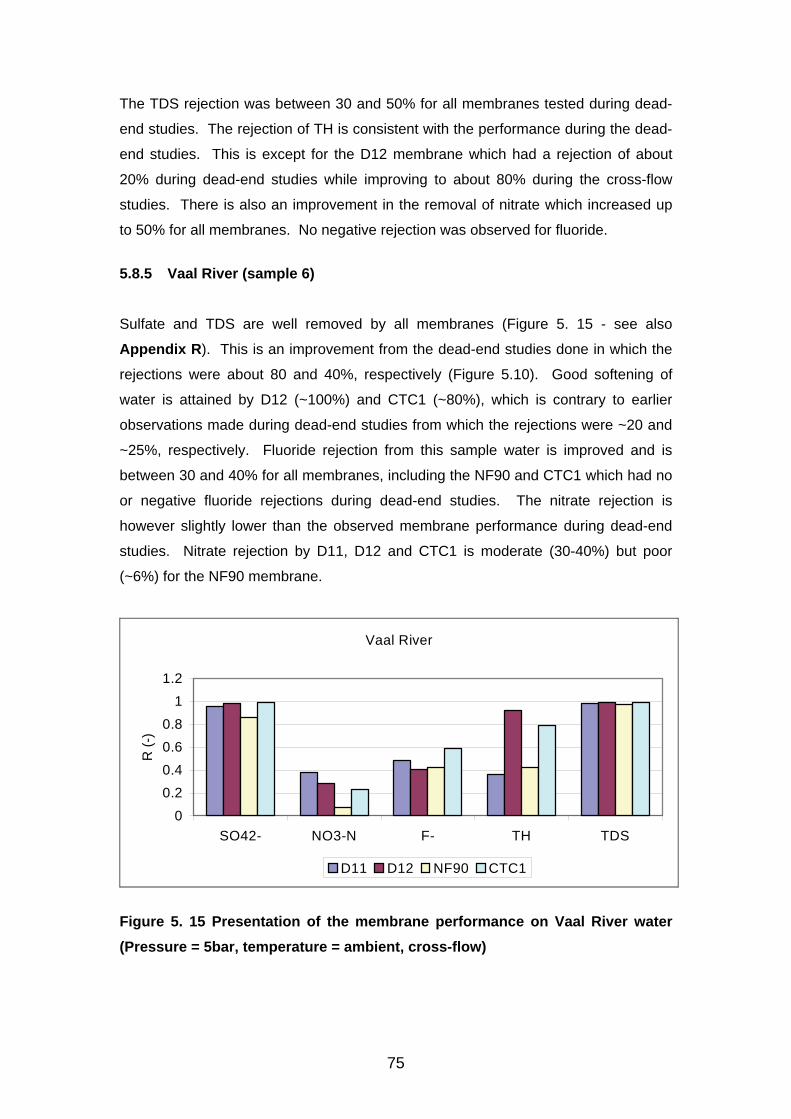
75
The TDS rejection was between 30 and 50% for all membranes tested during dead-
end studies. The rejection of TH is consistent with the performance during the dead-
end studies. This is except for the D12 membrane which had a rejection of about
20% during dead-end studies while improving to about 80% during the cross-flow
studies. There is also an improvement in the removal of nitrate which increased up
to 50% for all membranes. No negative rejection was observed for fluoride.
5.8.5 Vaal River (sample 6)
Sulfate and TDS are well removed by all membranes (Figure 5. 15 - see also
Appendix R). This is an improvement from the dead-end studies done in which the
rejections were about 80 and 40%, respectively (Figure 5.10). Good softening of
water is attained by D12 (~100%) and CTC1 (~80%), which is contrary to earlier
observations made during dead-end studies from which the rejections were ~20 and
~25%, respectively. Fluoride rejection from this sample water is improved and is
between 30 and 40% for all membranes, including the NF90 and CTC1 which had no
or negative fluoride rejections during dead-end studies. The nitrate rejection is
however slightly lower than the observed membrane performance during dead-end
studies. Nitrate rejection by D11, D12 and CTC1 is moderate (30-40%) but poor
(~6%) for the NF90 membrane.
Vaal River
0
0.2
0.4
0.6
0.8
1
1.2
SO42- NO3-N F- TH TDS
R (
-)
D11 D12 NF90 CTC1
Figure 5. 15 Presentation of the membrane performance on Vaal River water
(Pressure = 5bar, temperature = ambient, cross-flow)
76
5.9 Summary and Conclusion
The aim of this investigation was to evaluate a cross-flow nanofiltration membrane
unit and process for the removal of the divalents/multivalents (sulfate, total hardness,
total dissolved solids) and the monovalents (nitrate and fluoride). The separation
principle of such a process is based on molecular size exclusion and ionic (charge)
exclusion. Compared to reverse osmosis membranes, which indiscriminately
exclude almost all dissolved solids, regardless of their charge, nanofiltration
membranes remove the high valence ions (co-ions) mostly whilst selectively/partly
retaining the monovalents. In the treatment of rural water, the membranes were
successful in removing sulfate and in some cases effectively softened the sample
waters. The monovalent fluoride and nitrate were, however, retained average to poor
depending on the different compositions of the rural water.
During dead-end mode studies, NF70, TFC-S, D11 and TFC-SR membranes showed
good fluoride retentions for varying water samples. NF70 could reduce fluoride in the
Lerome rural water from about 4ppm to less than 1ppm (~76%) whilst permeation
with TFC-ULP was even less than 0.5ppm fluoride (91%). Although it yielded
negative fluoride rejection and even poor fluoride rejection for Haaskraal, Ledig and
Vaal River sample water, TFC-S showed satisfactory fluoride rejection for the
Lerome sample water.
Nitrate contents in all the sampled water were already within acceptable levels,
except at Haaskraal and Greenside. Still, when nanofiltered, only NF70 could show
satisfactory nitrate retention. Most other membranes showed little or negative
rejections. Appendix N and Appendix S shows detailed membrane performance for
each ionic component and sample water. The NF70 membrane can be
recommended for further investigation and use in rural water treatment due to its
overall retention capacity, even though (as also shown in previous work [7]) it shows
reverse osmosis tendencies by rejecting almost all components. The TFC-S and
TFC-SR membranes also have potential for selected cases of rural water treatment.
The high sulfate rejection by all membranes confirms that the membranes have a
negative surface charge. To improve the removal of other pollutants, a combination
of these membranes with the available positive NF and/or inorganic membranes can
be used.

77
Characterization by single or even binary salt mixtures cannot be used to predict
“real” performance of the membrane since it will be affected by the composite water it
is in contact with. Furthermore, it cannot be assumed that if a membrane improves
water quality of one contaminated site that it will do the same for other sites. As soon
as ion composition and composition of sampled water changes during treatment,
selectivity is drastically influenced. Each membrane has to be tested (screened) and
optimized for use for each site.
Generally, the nanofiltration membranes performed better in removing divalents
(especially anions) than monovalents for all sample water compositions. However,
some divalents, especially cations, were not so well retained, depending on the
nature of the membrane and the composition of the sample feed.
The unacceptable water quality (intended for drinking and food preparation) of
Lerome (purple) was not improved by any of the membranes. The same can be said
for the Ledig water. The Haaskraal water was in any case ideal so there was no
difference brought about by the membranes (Table 5. 8). The moderate fluoride level
at Vaal River is slightly improved to marginal quality.

78
Table 5. 8 Water classification (fluoride) before and after treatment by various
nanofiltration membranes
Fluoride
Lerome Ledig Haaskraal Vaal River
[F]o = 5.8 [F]o = 7.2 [F]o = 0.2 [F]o = 2.7
Brin
e
Product Brin
e
Product Brin
e
Product Brin
e
Produc
t
D11
Drinking (H)
Drinking (A)
Food
preparation
Bathing
Laundry
P P P P B B R Y
B B B B B B B B
P P P P B B R Y
B B B B B B B B
B B B B B B B B
D12
Drinking (H) P P P P B B R Y
Drinking (A) B B B B B B B B
Food
preparation
P P P P B B R Y
Bathing B B B B B B B B
Laundry B B B B B B B B
NF
90
Drinking (H) P P P P B B R Y
Drinking (A) B B B B B B B B
Food
preparation
P P P P B B R Y
Bathing B B B B B B B B
Laundry B B B B B B B B
CT
C1
Drinking (H) P P P P B B R Y
Drinking (A) B B B B B B B B
Food
preparation
P P P P B B R Y
Bathing B B B B B B B B
Laundry B B B B B B B B
H = Health, A = Aesthetic, B = Blue, G = Green, Y = Yellow, R = Red, and P = Purple.
79
1. McCaffrey, L. P. (1993). The Geohydrology of Pilanesburg. M.Sc. dissertation,
University of the Witwatersrand, Johannesburg, South Africa.
2. McCaffrey, L. P., Harris, C and Willis, J.P. (1996). An occurrence of calcites,
stontianites and ankerite in the Pilanesburg Complex, North West Province,
South Africa. S Afr. J.Geol., 99: 33 – 36.
3. Çengelogu, Y., Kir, E., and Ersöz, M. (2002). Removal of fluoride from aqueous
solution by using red mud. Separation and Purification Technology, 28: 81 –
86.
4. South Africa Bureau of Standards (2001) South African Standards,
Specification 241-1984: Drinking Water. Edition 5, SABS, Pretoria.
5. Water Research Commission (1998) Quality of domestic water supplies, vol 1
Assessment Guide. Water Research Commission Report TT101/88, WRC,
Pretoria.
6 Modise, S.J.(2003) South African rural water, Ph.D. thesis, Potchefstroom
University for CHE, Potchefstroom, South Africa.
7. Visser, T.J.K., Modise, S.J., Krieg, H.M. and Keizer, K. (2000) The removal of
acid sulfate pollution by nanofiltration. Desalination, 140: 79 – 86.
80
6 Evaluation and recommendations
The main findings of the characterization of the membranes, and their performance on the
rejection of selected electrolytes and rural water samples are given. Finally, some
recommendations for further research is presented.
6.1 Evaluation
The global importance of clean water cannot be over-emphasized. Everywhere
institutions and organisations have begun reviewing provisions of safe and clean water.
The South African response has been the enactment of the National Water Act 36 of 1998,
which guarantees safe water by guarding against pollution with the intention to protect and
conserve water. If implemented properly, many rural areas will benefit by getting clean
water that is free from hazardous organic or inorganic components.
In view of the aforementioned, the high levels of fluoride (around the Pilanesberg) and
nitrate (around Moretele and Kudumane districts) within the North West region cannot be
left unattended. The high levels of fluoride result is mottling of the teeth and skeletal
fluorosis, which is clearly noticeable within the Pilanesberg region.
Sampling in the selected regions of the North West Province was done to gain an
understanding of the extent of pollution, especially in rural areas. Fluoride levels were
found to be high in the greater Pilanesberg area and in some parts of the Mafikeng region.
Other chemical components, including nitrates, were found to be within the acceptable
limits. Sulfate concentration was high only at the Vaal River, downstream from the gold
mines.
During characterization, D11, D12 and TFC-SR showed high water fluxes and
permeabilities. TFC-SR membrane had higher solute fluxes than TFC-S. The lowest
solute fluxes were observed for NF70, NF90 and TFC-HR. NF70, NF90 and TFC-S
displayed more properties of reverse osmosis (RO) than nanofiltration (NF) characteristics
with low permeability.
Various nanofiltration membranes were tested for their ability to remove the chemical
components from the sampled water of Lerome, Ledig, Haaskraal and the Vaal River.
Sulfate was efficiently removed by all membranes (confirming previous findings on the

81
removal of sulfate ions from acid mine water [1]). However, not all membranes could
satisfactorily remove total hardness. Fluoride was also not retained well by all
membranes. Nitrate was retained well by the NF70 membrane only. The other
membranes showed poor, and in some cases even negative retention. In general, the
FilmTec® NF70, and the Koch Membrane Systems’ TFC-S and TFC-SR showed relative
good removal of both mono- and divalent chemical components. The model solution
(single and mixture salts) studies, however, cannot be used to predict the membrane
behaviour in rural water treatment. One cannot even deduce that the membrane will
perform the same way for different water sources.
6.2 Highlights
Fluoride in the Rustenburg area is at an unacceptable level especially around the
Pilanesberg region. Some boreholes around the Mafikeng area have fluoride levels
just above 1ppm which can be a cause of concern as this area is not usually
associated with these pollutants;
Nitrate levels in the sampled areas was not a health threat except in one private
borehole of Rustenburg’s Greenside area (sample 13);
Of all the sampled points, sulfate levels were high at the Vaal river, downstream of
some gold mines;
Sulfate removal by NF-membranes was excellent (as also observed in mine water
treatment [1]);
NF-membranes behave differently for different rural water compositions;
Characterization of nanofiltration membranes does not necessarily predict how they
will perform with polluted water as removal of pollutants depend largely on the
composition of the water; i.e. the presence and concentration of other ions;
NF70 can be recommended as it could remove most salts from both prepared
solutions and polluted water;
82
D11, D12 and CTC-1 can be recommended with restrictions (due to its limited nitrate
and fluoride removal);
6.3 General discussions
The NF-membrane process offers a technique that can be used for rural water treatment.
If the correct membrane is chosen for a specific locality, then sulfate, fluoride, and nitrate
levels can be reduced. However, screening tests have to be done initially to select the
proper membrane. The dead-end NF set-up built in this study is ideal for such membrane
screening.
The scattered homes in the rural areas make it difficult for the treatment of water by NF-
membranes. The difficulty is enhanced by the fact that most boreholes in the affected
areas are private and in backyards and it will be difficult to closely monitor all of them.
Hence, the membrane process can only be effective if the water is treated by the local
(central) water authority and then distributed to the consumers. In so doing, the unit could
benefit more residents than when it was placed at only a specific borehole. Such a unit
might, however, be necessary in affected areas, forming a part of an integrated rural
development. The other possible hindrance of a membrane application in the rural areas
is the cost of technology transfer, maintenance and the availability of skilled labour. It
should be noted that even though the unit might be moved to another community, it will be
the owner’s responsibility to make sure that it does not become a white elephant.
Water treated by NF-membranes, has value added to it. Such an addition of value would
necessitate that the communities pay for the product. Such an approach might be difficult
in the poverty stricken rural areas. Besides, rural communities have most of the water
sources right in the yards, and as long as they can remember they never had to pay for
water. Part of the solution to this addition of value will therefore require direct involvement
of the communities so that they can take ownership of the activities, including the pricing
of the water. It would be a futile exercise to do any of this membrane water treatment
tests without the involvement of the local community.
The brine, as one of the membrane process products, needs to be disposed of or reused.
It will therefore be important to study the area for possible wastewater reuse. The options
that can be considered in such areas are irrigation, livestock watering, development of
mini-parks, etc.
83
6.4 Recommendations and further research
Private boreholes in the backyards of the rural areas need constant quality
assessment, especially by the water-supply authorities. Not all boreholes need to be
monitored, but they can be selected in such a way that they are representative of all
other boreholes. To do this, a strategic assessment and monitoring plan might be
necessary over a limited number of years.
There is a need for further monitoring of nitrate and fluoride levels; including or
extending the current sampling regions. This necessitates collaboration with the
Health Department on issues like the effects of high levels on the consumers.
Membrane characterization methods would need to be quantified and systematized as
a protocol so that there is uniformity and comparability when characterizing
membranes. Also, much more and better understanding of the mechanism of
separation as well as the influence of other ions is required before any prediction of
membrane performance is possible.
Parameters that might hinder optimum water treatment by nanofiltration membranes
(e.g. fouling) need intense investigation.
The use of nanofiltration membranes have a backlog of poor monovalent rejections.
This however, is not a limitation to optimally use the built cross-flow unit for intense
nanofiltration studies.
Campaigns on the importance and scarcity of water need to be run to educate all
South Africans. In the many areas visited; leaking taps, unattended running water and
overflowing water from tanks were found. In many cases the residents themselves did
not know what to do with such problems (even where to report them). Water reuse (for
washing cars, gardening, sanitation, etc.) has to be encouraged.
References
1. Visser, T.J.K, Modise S.J., Krieg, H.M. and Keizer, K. (2000) The removal of
acid sulfate pollution by nanofiltration. Desalination, 140: 79-86.

84
Ap
pen
dix
A S
olu
te f
lux
of
vari
ou
s m
od
el s
olu
tio
ns
at d
iffe
ren
t tr
ans-
mem
bra
ne
pre
ssu
res
S
olu
te f
lux
(10-6
m.s
-1)
Mem
bra
ne
Co
nce
ntr
atio
n
(pp
m)
NaC
l H
2SO
4
5 10
15
20
5
10
15
20
TF
C-S
20
X
X
X
X
X
X
X
X
50
X
X
X
X
X
X
X
X
100
X
X
0.47
0.
63
X
X
2.30
3.
33
200
X
X
0.27
0.
39
X
X
2.89
3.
71
TF
C-S
R
20
18.9
34
.5
52.1
71
.0
19.4
34
.9
52.5
70
.2
50
19.5
36
.5
52.1
71
.0
20.3
37
.2
55.8
77
.2
100
19.7
36
.5
55.3
74
.4
21.3
38
.1
54.8
74
.4
200
20.0
36
.5
54.8
73
.5
20.4
38
.6
56.8
72
.7
TF
C-H
R
20
X
X
X
X
X
X
X
X
50
X
X
X
X
X
X
X
X
100
4.84
7.
97
10.6
13
.7
3.91
7.
66
11.9
15
.3
200
3.75
7.
18
10.6
14
.1
3.59
7.
18
11.1
14
.7
CT
C1
20
9.89
19
.1
26.9
38
.8
8.12
16
.1
23.9
30
.0
50
9.39
24
.5
36.3
50
.0
7.74
15
.3
23.0
32
.3
100
12.8
25
.6
37.0
37
.5
7.88
15
.7
22.6
35
.0
200
12.0
X
37
.0
50.4
8.
00
15.6
23
.6
33.5
NF
70
20
3.60
7.
84
11.4
15
.1
2.66
5.
31
8.13
10
.8
50
3.60
7.
00
11.0
14
.8
2.81
5.
31
8.28
12
.3
100
3.82
7.
63
11.4
15
.5
2.81
5.
47
8.59
11
.4
200
4.03
7.
63
11.4
15
.1
2.34
4.
84
7.03
10
.0
NF
90
20
3.39
8.
48
13.4
18
.2
2.43
5.
18
9.19
13
.6
50
4.24
8.
69
14.0
18
.7
2.43
5.
23
8.98
13
.8
100
3.18
6.
15
9.54
12
.7
2.41
5.
17
9.10
13
.7
200
3.39
7.
21
10.2
13
.8
2.43
5.
31
9.06
13
.3

85
App
endi
x A
(co
ntin
ued…
)
Vo
lum
e fl
ux
(10-6
m.s
-1)
Mem
bra
ne
Co
nce
ntr
atio
n
(pp
m)
CaS
O4
Na 2
SO
4
5 10
15
20
5
10
15
20
TF
C-S
20
X
X
X
X
X
X
X
X
50
X
X
X
X
X
X
X
X
100
X
X
0.25
0.
58
X
X
0.38
0.
66
200
X
X
0.41
0.
48
X
X
0.47
0.
53
TF
C-S
R
20
X
X
X
53.0
21
.5
39.8
56
.3
73.5
50
X
39
.3
55.8
71
.0
21.6
38
.6
54.8
69
.4
100
20.7
38
.6
54.6
67
.6
19.2
35
.3
50.0
61
.3
200
20.3
36
.2
50.0
59
.0
18.9
35
.1
48.8
61
.3
TF
C-H
R
20
3.59
7.
34
11.4
14
.7
3.52
7.
27
10.3
14
.2
50
3.59
7.
34
10.6
13
.9
3.56
7.
26
10.3
14
.6
100
3.75
7.
19
11.6
15
.8
3.54
7.
26
10.2
13
.8
200
3.44
6.
88
10.5
14
.4
3.86
7.
19
10.3
13
.7
CT
C1
20
8.04
15
.8
23.3
31
.5
7.74
15
.4
22.9
30
.9
50
7.76
15
.7
22.3
31
.0
8.23
14
.8
23.5
31
.2
100
8.88
16
.0
23.6
31
.3
7.68
15
.7
23.0
30
.7
200
7.32
14
.9
22.4
32
.3
7.69
15
.9
23.4
31
.1
NF
70
20
2.66
5.
63
8.75
11
.9
2.74
6.
01
9.13
12
.1
50
2.97
5.
94
9.22
12
.2
2.40
6.
09
9.15
12
.6
100
2.97
5.
63
8.91
12
.5
2.42
6.
12
9.13
11
.9
200
2.81
5.
63
8.75
11
.3
2.41
6.
03
9.13
12
.4
NF
90
20
2.43
5.
51
7.58
9.
62
2.82
5.
60
8.32
11
.2
50
2.42
5.
43
7.54
9.
60
2.85
5.
66
8.45
11
.2
100
2.43
5.
49
7.53
9.
58
2.81
5.
91
8.38
11
.7
200
2.43
5.
47
7.53
9.
61
2.84
5.
73
8.36
10
.8

86
Appendix B Retention of NaNO3 solutions on different membranes
NaNO3 on CTC-1
0.00
0.20
0.40
0.60
0.80
0 5 10 15 20 25
pressure (bar)
R (
-)
20 mg/l 50 mg/l 100 mg/l 200 mg/l
NaNO3 on TFC-SR
0.000.100.200.300.400.500.60
0 5 10 15 20 25
pressure (bar)
R (
-)
20 mg/l 50 mg/l 100 mg/l 200 mg/l
NaNO3 on TFC-HR
0.00
0.20
0.40
0.60
0.80
1.00
0 5 10 15 20 25
pressure (bar)
R (
-)
20 mg/l 50 mg/l 100 mg/l 200 mg/l
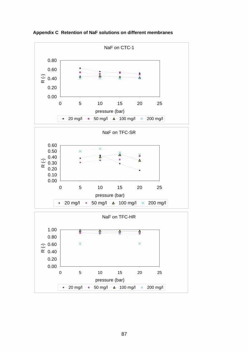
87
Appendix C Retention of NaF solutions on different membranes
NaF on CTC-1
0.00
0.20
0.40
0.60
0.80
0 5 10 15 20 25
pressure (bar)
R (
-)
20 mg/l 50 mg/l 100 mg/l 200 mg/l
NaF on TFC-SR
0.000.100.200.300.400.500.60
0 5 10 15 20 25
pressure (bar)
R (
-)
20 mg/l 50 mg/l 100 mg/l 200 mg/l
NaF on TFC-HR
0.00
0.20
0.40
0.60
0.80
1.00
0 5 10 15 20 25
pressure (bar)
R (
-)
20 mg/l 50 mg/l 100 mg/l 200 mg/l
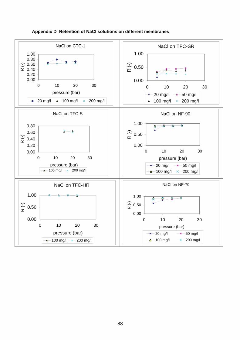
88
Appendix D Retention of NaCl solutions on different membranes
NaCl on CTC-1
0.000.200.400.600.801.00
0 10 20 30
pressure (bar)
R (
-)
20 mg/l 100 mg/l 200 mg/l
NaCl on TFC-SR
0.00
0.50
1.00
0 10 20 30
pressure (bar)
R (
-)
20 mg/l 50 mg/l
100 mg/l 200 mg/l
NaCl on TFC-S
0.00
0.20
0.40
0.60
0.80
0 10 20 30
pressure (bar)
R (
-)
100 mg/l 200 mg/l
NaCl on NF-90
0.00
0.50
1.00
0 10 20 30
pressure (bar)
R (
-)
20 mg/l 50 mg/l
100 mg/l 200 mg/l
NaCl on TFC-HR
0.00
0.50
1.00
0 10 20 30
pressure (bar)
R (
-)
100 mg/l 200 mg/l
NaCl on NF-70
0.00
0.50
1.00
0 10 20 30
pressure (bar)
R (
-)
20 mg/l 50 mg/l
100 mg/l 200 mg/l
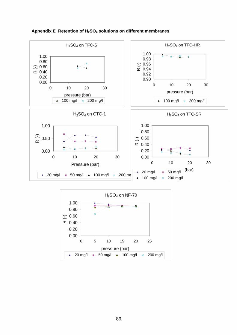
89
Appendix E Retention of H2SO4 solutions on different membranes
H2SO4 on TFC-S
0.000.200.400.600.801.00
0 10 20 30
pressure (bar)
R (
-)
100 mg/l 200 mg/l
H2SO4 on CTC-1
0.00
0.50
1.00
0 10 20 30
Pressure (bar)
R (
-)
20 mg/l 50 mg/l 100 mg/l 200 mg/l
H2SO4 on TFC-HR
0.900.920.940.960.981.00
0 10 20 30
pressure (bar)
R (
-)
100 mg/l 200 mg/l
H2SO4 on TFC-SR
0.00
0.20
0.40
0.60
0.80
1.00
0 10 20 30
pressure (bar)
R (
-)
20 mg/l 50 mg/l
100 mg/l 200 mg/l
H2SO4 on NF-70
0.00
0.20
0.40
0.60
0.80
1.00
0 5 10 15 20 25
pressure (bar)
R (
-)
20 mg/l 50 mg/l 100 mg/l 200 mg/l

90
Appendix F Electrical connections to pump 1. Electrical connections to pump 1 (sandfilter pump, operating pressure = ~1
bar)
8
NC
N
4
1
32
25
28
13
1
12
From L2 in Pump3
3
Red
19
2
N
5
30
N
1
2
22Overload
30
OnYellow
6
7
Green
Pump2
White
Torelay
9
31
29
13
2
StandBy
Pump1
20L1
Timer
22
Override
21
4
N
19
3
N
4
N
21
24
L1
3
Low
21
7
4
24
N
14
4
4
10
26Thickwire
18
15
17
31
5
14
5
29
15 23
1
Relay2
23
Red
11
Relay
27
18
Twist Button StartCircle
N
Override
Pump1
4
7
6
6
8
204
From L1in Pump3
N
29
28
Tank1
Stop
8
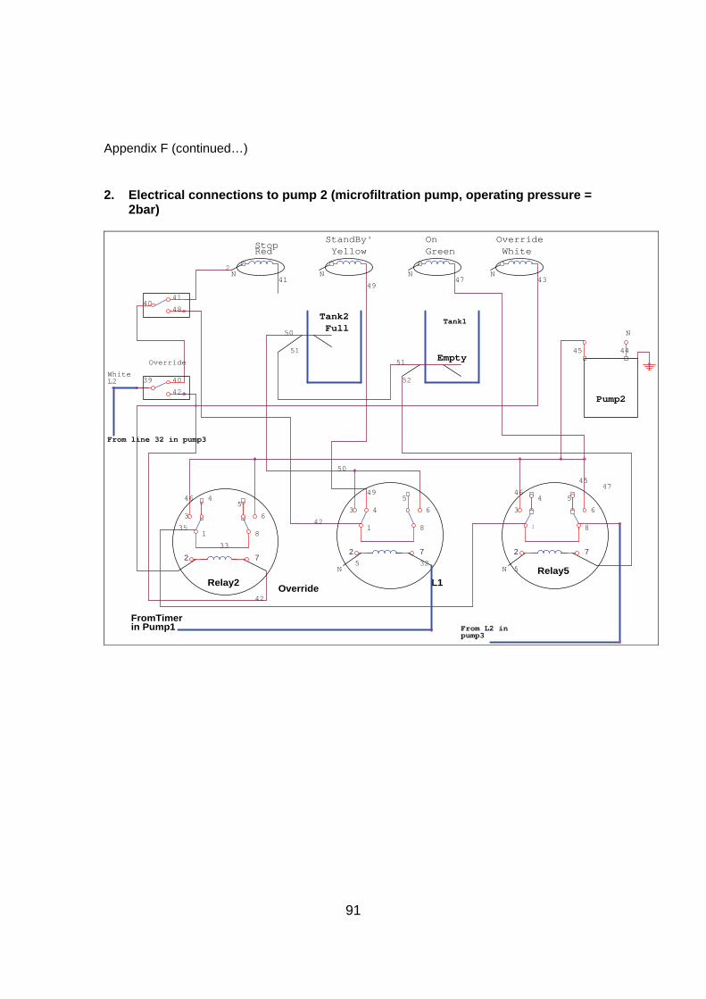
91
Appendix F (continued…) 2. Electrical connections to pump 2 (microfiltration pump, operating pressure =
2bar)
4
52
42
Tank2
4
Full
2
6
Empty
1
5
50
From L2 inpump3
Override
43
8
7
WhiteL2
StandBy'
32
2
From line 32 in pump3
44
40
35
41
2
63
N
40
2
N
Relay5
Green
39
White
N
45
6
5
47
StopOn
47
L1
42
45
1
Relay2
42
7
4
Tank1
Pump2
N
3
46
N
3
5
Override
Override
49
8
Red
7
51
5
Yellow
N
8
FromTimerin Pump1
1
5
49
48
33
51
46
N41
50
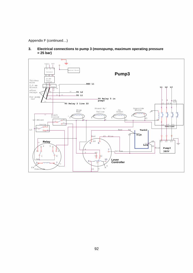
92
Appendix F (continued…) 3. Electrical connections to pump 3 (monopump, maximum operating pressure
= 25 bar)
63
L363
58
7
L3
TO Relay 5 inpump2
Stand By'
66
64
3
7
L1
NYellow
L3
58
L3
TO L2
L3
Isolator
Pump3
39
L1
60
62
4
Relay
30 Amp
N
1
2.0 mmdirect
N
L2
56
8 10
L2
6
L1
5
Supply 380V
2
6
Yellow
12
Override
Low
9
3
High
39
Tank2
Blue
8
Circuit breaker
N
Blue
L3
64
6
afterrelays
Red
N
Earth
Stop
L3
56
L2
65
Neutral Block
53
N 61
StartCircle
7
60
L1
L1
6
5
60 Amp
62
On
61 Pump3
L1
L2
L2
55
9
12
White
2
Green
3
L3
22
65
53
(Blue)
7
for pump 1&2
59
Leakage
380V
N
4
L2
L3
10
59
Red
Override
Thickerwire
Override
1
RED L1
Overload
55
LeverController
L1
54
54
L2
TO L1
6
L1
L1
62
Red
TO Relay 2 line 22
66
11
8

93
Appendix G Water quality from various sampling sites within the North West Province on four different occasions
Sampling 1: Beginning of rainy season (BRS) F-
(mg.l-1) NO3-N (mg.l-1)
SO42-
(mg.l-1) Cl- (mg.l-1)
Na+
(mg.l-1) TH (mg.l-1)
Cu2+ (mg.l-1)
TDS (mg.l-1)
pH
Kle
rksd
orp
regi
on
Mooi River 1 1.4 1.6 23 18 131 67 0.08 1201 6.6 Potch Univ. 2 1.0 2.3 19 24 42 83 0.06 198 6.6 Boitshoko School 2a 0.8 0.0 8 21 32 38 0.03 1341 7.3 Sarafina 2b 0.7 0.0 9 19 56 38 0.01 1800 7.8 Rietspruit 3 0.2 5.4 21 11 90 23 0.04 305 7.1 Taaiboschspruit 4 1.7 6.2 72 12 140 42 0.03 315 6.9 Orkney Vaal 6 2.7 1.6 112 41 210 18 0.02 1108 7.3
Kos
ter
regi
on
Kaallagte 1 8a 0.3 1.1 0 6 71 57 0.03 299 7.0 Kaallagte 2 8b 0.2 0.0 0 0 39 17 0.03 600 6.5 Rhenosterfontein 9 0.0 1.7 64 5 83 15 1.41 330 6.3 Tlholego 1 10a 0.9 1.5 63 7 86 17 1.40 1036 6.4 Tlholego 2 10b 0.4 0.0 60 0 79 47 0.19 1131 7.4 Tlholego 3 10c 0.4 0.0 61 0 68 60 0.93 1203 7.1 Tlholego 4 10d 0.2 0.0 63 0 91 76 0.81 1347 7.1 Roodewal 11 1.0 0.2 9 5 23 83 0.04 1263 6.8
Rus
tenb
urg
regi
on
Rietvlei 12 0.0 2.8 5 5 36 57 0.08 1098 6.9 Greenside 13 1.0 14 0 26 117 58 0.10 1018 6.4 Mogwase 14 2.6 0.1 138 10 339 72 0.15 5280 6.3 Beestekraal 15 1.1 0.2 60 69 143 41 0.08 2936 6.3 Bakgatla 20 3.8 2.5 61 96 31 47 0.21 591 6.9 Lerome 1 13a 5.5 0.0 0 16 29 35 0.14 2300 7.3 Lerome 2 21 4.5 1.5 59 70 19 59 0.23 893 7.0 Lerome 3 25 3.3 1.2 50 36 86 51 0.01 899 7.6 Ledig 1 23 7.2 1.0 20 40 113 18 0.13 831 7.5 Ledig 2 22 3.3 0.7 50 24 30 38 0.14 1200 6.8 Lefaragatlhe 24 0.2 4.8 29 42 67 21 0.06 583 6.3
Maf
iken
g Lichtenburg 5 1.1 2.3 0 28 178 21 0.03 851 6.6
Mmabatho 16 0.6 0.8 15 63 73 56 0.09 649 6.3 Letlamoreng 1 17 1.8 0.8 62 52 138 119 0.09 1093 6.4 Letlamoreng 2 18 1.8 0.8 30 71 93 137 0.10 2999 7.1
TH = Total hardness as CaCO3, TDS = Total dissolved solids

94
Appendix G (continued…)
Sampling 2: Middle of rainy season (MRS) F-
(mg.l-1) NO3-N (mg.l-1)
SO42-
(mg.l-1) Cl-
(mg.l-1) Na+
(mg.l-1) TH (mg.l-1)
Cu2+ (mg.l-1)
TDS (mg.l-1)
pH
Kle
rksd
orp
regi
on
Mooi River 1 0.30 0.45 34 0.3 67 35 0.05 1300 6.1 Potch Univ. 2 0.21 6.30 79 0.1 83 13 0.05 531 7.2 Boitshoko School 2a 0.00 0.00 42 0.1 81 18 0.06 900 6.4 Sarafina 2b 0.00 0.00 19 0.1 62 16 0.07 1356 6.3 Rietspruit 3 0.00 2.71 21 0.1 78 21 0.06 831 6.5 Taaiboschspruit 4 0.00 3.08 64 2.3 131 31 0.06 631 6.3 Orkney Vaal 6 0.00 4.11 163 3.9 190 44 0.03 631 6.5
Kos
ter
regi
on
Kaallagte 1 8a 0.07 1.40 35 0.6 82 28 0.06 636 6.8 Kaallagte 2 8b 0.00 0.00 29 0.5 98 33 0.03 1039 6.1 Rhenosterfontein 9 0.00 0.00 24 0.7 72 57 0.05 843 7.8 Tlholego 1 10a 0.00 0.00 56 0.3 168 58 0.05 869 6.3 Tlholego 2 10b 0.01 0.00 52 0.0 156 54 0.05 999 5.9 Tlholego 3 10c 0.03 0.00 51 0.0 170 60 0.05 831 6.4 Tlholego 4 10d 0.05 1.36 48 0.0 166 51 0.03 1103 6.3 Roodewal 11 0.23 0.00 30 0.1 62 44 0.06 898 6.8
Rus
ten
burg
re
gion
Rietvlei 12 0.00 3.08 8 0.6 63 37 0.06 1090 6.5 Greenside 13 0.60 14.7 10 1.3 215 52 0.09 1534 6.6 Mogwase 14 0.30 0.79 108 0.8 336 39 0.14 3606 6.6 Beestekraal 15 0.21 0.29 43 0.8 123 43 0.03 5311 6.9 Bakgatla 20 4.72 7.45 111 1.9 286 93 0.01 906 6.4 Lerome 1* 13a - - - - - - - - - Lerome 2 21 3.91 6.28 41 1.3 135 46 0.08 1100 6.3 Lerome 3 25 3.50 8.61 31 0.6 86 19 0.01 837 7.6 Ledig 1 23 8.30 0.59 68 0.7 138 35 0.03 600 7.2 Ledig 2 22 5.10 5.11 58 0.1 142 26 0.03 1109 6.3 Lefaragatlhe 24 0.99 3.79 70 0.5 168 73 0.03 543 6.3
Maf
iken
g
Lichtenburg 5 0.26 3.11 59 1.4 122 8 0.05 942 7.3 Mmabatho 16 0.00 1.49 53 0.1 128 33 0.06 743 6.5 Letlamoreng 1 17 0.08 0.00 27 0.0 139 50 0.01 1099 6.6 Letlamoreng 2 18 0.46 0.70 31 0.1 193 30 0.01 2046 6.5
TH = Total hardness as CaCO3, TDS = Total dissolved solids * not sampled as no water could be pumped out.

95
Appendix G (continued…)
Sampling 3: Beginning of dry season (BDS) F-
(mg.l-1) NO3-N (mg.l-1)
SO42-
(mg.l-1) Cl-
(mg.l-1) Na+
(mg.l-1) TH (mg.l-1)
Cu2+ (mg.l-1)
TDS (mg.l-1)
pH
Kle
rksd
orp
regi
on
Mooi River 1 0.3 14.9 51 21 128 51 0 1138 6.0 Potch Univ. 2 0.2 4.54 83 24 53 80 0 195 7.1 Boitshoko School 2a 0.3 5.65 39 23 28 0 0 1256 6.8 Sarafina 2b 0.3 1.11 48 19 51 0 0.01 3042 6.4 Rietspruit 3 0.1 0.77 28 30 88 40 0 415 6.3 Taaiboschspruit 4 0.6 5.65 83 18 133 23 0 467 6.3 Orkney Vaal 6 0.3 0.88 246 48 198 63 0 1280 6.8
Kos
ter
regi
on
Kaallagte 1 8a 0.3 2.51 56 13 61 18 0 357 6.3 Kaallagte 2 8b 0.4 2.12 55 9 43 10 0.12 817 7.5 Rhenosterfontein 9 0.6 1.54 60 21 91 15 0 344 6.9 Tlholego 1 10a 0.1 2.15 73 16 84 31 1.46 1882 6.8 Tlholego 2 10b 0.1 1.19 69 22 71 0 1.41 1642 7.1 Tlholego 3 10c 0.1 1.85 83 6 79 0 0.81 1839 6.3 Tlholego 4 10d 0.2 0.63 71 23 93 0 0 1798 6.4 Roodewal 11 0.1 1.24 56 71 19 53 0 1149 6.4
Rus
ten
burg
re
gio
n
Rietvlei 12 0.2 2.10 63 16 29 55 0.93 1121 7.3 Greenside 13 0.9 13.1 81 17 114 78 0.96 1753 6.3 Mogwase 14 6.8 7.05 59 29 300 39 0.09 6468 6.3 Beestekraal 15 0.6 1.38 183 83 123 43 0.05 3835 6.3 Bakgatla 20 0.6 3.82 28 27 33 21 0 642 6.9 Lerome 1 13a 0.1 2.87 47 42 31 0 0.01 2367 6.5 Lerome 2 21 4.5 2.28 51 68 21 17 0.06 983 6.4 Lerome 3 25 3.8 3.12 55 61 84 11 0 839 6.3 Ledig 1 23 7.4 3.07 63 55 116 23 0 685 6.3 Ledig 2 22 5.3 2.21 57 93 25 46 0 1035 6.2 Lefaragatlhe 24 0.3 0.79 24 96 66 31 0 781 6.1
Maf
ike
ng
Lichtenburg 5 0.5 2.37 58 28 102 60 0 964 7.6 Mmabatho 16 0.5 2.64 69 197 86 113 0.03 748 6.7 Letlamoreng 1 17 0.3 0.75 53 402 125 81 0.04 1396 6.4 Letlamoreng 2 18 0.2 0.95 21 451 92 128 0 3373 7.2
TH = Total hardness as CaCO3, TDS = Total dissolved solids
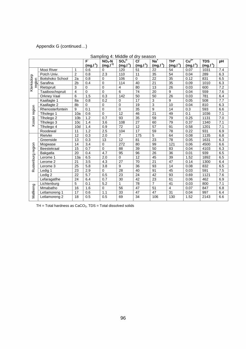
96
Appendix G (continued…)
Sampling 4: Middle of dry season F-
(mg.l-1) NO3-N (mg.l-1)
SO42-
(mg.l-1) Cl- (mg.l-1)
Na+
(mg.l-1) TH* (mg.l-1)
Cu2+ (mg.l-1)
TDS (mg.l-1)
pH
Kle
rksd
orp
regi
on
Mooi River 1 0.6 0 120 51 22 54 0.07 1031 7.4 Potch Univ. 2 0.8 2.3 110 11 35 54 0.04 289 6.3 Boitshoko School 2a 0.8 0 106 0 22 35 0.12 831 6.5 Sarafina 2b 0.4 0 114 40 21 35 0.09 1010 6.3 Rietspruit 3 0 0 4 80 13 26 0.03 600 7.2 Taaiboschspruit 4 0 0 6 74 20 9 0.04 559 7.6 Orkney Vaal 6 1.5 0.3 142 50 50 26 0.03 781 6.4
Kos
ter
regi
on
Kaallagte 1 8a 0.8 0.2 0 17 3 9 0.05 508 7.7 Kaallagte 2 8b 0 0 0 19 3 10 0.04 810 6.3 Rhenosterfontein 9 0.1 0 0 35 9 14 0.3 593 6.6 Tlholego 1 10a 0.6 0 12 46 21 49 0.1 1036 7.1 Tlholego 2 10b 1.2 0.7 93 35 59 79 0.25 1131 7.0 Tlholego 3 10c 1.4 3.6 108 27 60 79 0.37 1340 7.1 Tlholego 4 10d 1.4 0.9 72 12 57 91 0.58 1201 7.1 Roodewal 11 1.2 2.5 104 17 59 78 0.22 931 6.9
Rus
ten
burg
re
gion
Rietvlei 12 0.3 2.0 7 175 5 64 0.08 1135 6.8 Greenside 13 0.3 13 12 81 23 78 0.05 1631 6.3 Mogwase 14 3.4 0 272 80 99 121 0.06 4500 6.6 Beestekraal 15 0.7 0 88 39 50 83 0.04 4103 6.3 Bakgatla 20 0.4 4.7 95 96 26 36 0.01 939 6.5 Lerome 1 13a 6.5 2.0 0 12 45 39 1.52 1892 6.5 Lerome 2 21 3.5 4.3 27 70 21 47 0.14 1300 6.4 Lerome 3 25 5.8 3.8 9 36 93 14 0.08 832 6.5 Ledig 1 23 2.9 0 28 40 91 45 0.03 591 7.5 Ledig 2 22 5.7 0.5 23 24 42 93 0.69 1121 7.6 Lefaragatlhe 24 6.4 0.7 30 42 23 61 0.06 462 6.9
Maf
ike
ng
Lichtenburg 5 0.1 5.2 1 78 7 41 0.03 800 7.1 Mmabatho 16 1.6 0 56 47 51 4 0.07 847 6.8 Letlamoreng 1 17 0.6 1.1 33 47 47 31 0.04 997 6.4 Letlamoreng 2 18 0.5 0.5 69 34 106 130 1.52 2143 6.6
TH = Total hardness as CaCO3, TDS = Total dissolved solids
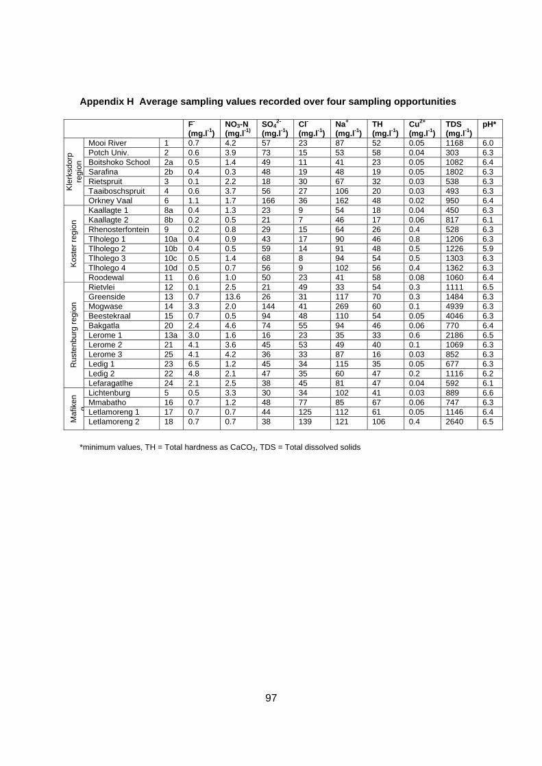
97
Appendix H Average sampling values recorded over four sampling opportunities
F- (mg.l-1)
NO3-N (mg.l-1)
SO42-
(mg.l-1) Cl-
(mg.l-1) Na+
(mg.l-1) TH (mg.l-1)
Cu2+ (mg.l-1)
TDS (mg.l-1)
pH*
Kle
rksd
orp
regi
on
Mooi River 1 0.7 4.2 57 23 87 52 0.05 1168 6.0 Potch Univ. 2 0.6 3.9 73 15 53 58 0.04 303 6.3 Boitshoko School 2a 0.5 1.4 49 11 41 23 0.05 1082 6.4 Sarafina 2b 0.4 0.3 48 19 48 19 0.05 1802 6.3 Rietspruit 3 0.1 2.2 18 30 67 32 0.03 538 6.3 Taaiboschspruit 4 0.6 3.7 56 27 106 20 0.03 493 6.3 Orkney Vaal 6 1.1 1.7 166 36 162 48 0.02 950 6.4
Kos
ter
regi
on
Kaallagte 1 8a 0.4 1.3 23 9 54 18 0.04 450 6.3 Kaallagte 2 8b 0.2 0.5 21 7 46 17 0.06 817 6.1 Rhenosterfontein 9 0.2 0.8 29 15 64 26 0.4 528 6.3 Tlholego 1 10a 0.4 0.9 43 17 90 46 0.8 1206 6.3 Tlholego 2 10b 0.4 0.5 59 14 91 48 0.5 1226 5.9 Tlholego 3 10c 0.5 1.4 68 8 94 54 0.5 1303 6.3 Tlholego 4 10d 0.5 0.7 56 9 102 56 0.4 1362 6.3 Roodewal 11 0.6 1.0 50 23 41 58 0.08 1060 6.4
Rus
ten
burg
re
gio
n
Rietvlei 12 0.1 2.5 21 49 33 54 0.3 1111 6.5 Greenside 13 0.7 13.6 26 31 117 70 0.3 1484 6.3 Mogwase 14 3.3 2.0 144 41 269 60 0.1 4939 6.3 Beestekraal 15 0.7 0.5 94 48 110 54 0.05 4046 6.3 Bakgatla 20 2.4 4.6 74 55 94 46 0.06 770 6.4 Lerome 1 13a 3.0 1.6 16 23 35 33 0.6 2186 6.5 Lerome 2 21 4.1 3.6 45 53 49 40 0.1 1069 6.3 Lerome 3 25 4.1 4.2 36 33 87 16 0.03 852 6.3 Ledig 1 23 6.5 1.2 45 34 115 35 0.05 677 6.3 Ledig 2 22 4.8 2.1 47 35 60 47 0.2 1116 6.2 Lefaragatlhe 24 2.1 2.5 38 45 81 47 0.04 592 6.1
Maf
iken
g
Lichtenburg 5 0.5 3.3 30 34 102 41 0.03 889 6.6 Mmabatho 16 0.7 1.2 48 77 85 67 0.06 747 6.3 Letlamoreng 1 17 0.7 0.7 44 125 112 61 0.05 1146 6.4 Letlamoreng 2 18 0.7 0.7 38 139 121 106 0.4 2640 6.5
*minimum values, TH = Total hardness as CaCO3, TDS = Total dissolved solids
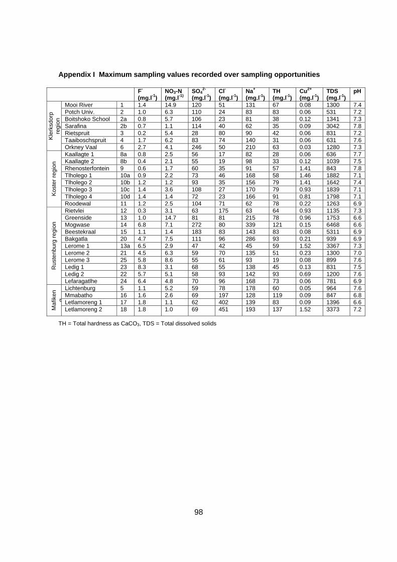
98
Appendix I Maximum sampling values recorded over sampling opportunities
F- (mg.l-1)
NO3-N (mg.l-1)
SO42-
(mg.l-1) Cl-
(mg.l-1) Na+
(mg.l-1) TH (mg.l-1)
Cu2+ (mg.l-1)
TDS (mg.l-1)
pH
Kle
rksd
orp
regi
on
Mooi River 1 1.4 14.9 120 51 131 67 0.08 1300 7.4 Potch Univ. 2 1.0 6.3 110 24 83 83 0.06 531 7.2 Boitshoko School 2a 0.8 5.7 106 23 81 38 0.12 1341 7.3 Sarafina 2b 0.7 1.1 114 40 62 35 0.09 3042 7.8 Rietspruit 3 0.2 5.4 28 80 90 42 0.06 831 7.2 Taaiboschspruit 4 1.7 6.2 83 74 140 31 0.06 631 7.6 Orkney Vaal 6 2.7 4.1 246 50 210 63 0.03 1280 7.3
Kos
ter
regi
on
Kaallagte 1 8a 0.8 2.5 56 17 82 28 0.06 636 7.7 Kaallagte 2 8b 0.4 2.1 55 19 98 33 0.12 1039 7.5 Rhenosterfontein 9 0.6 1.7 60 35 91 57 1.41 843 7.8 Tlholego 1 10a 0.9 2.2 73 46 168 58 1.46 1882 7.1 Tlholego 2 10b 1.2 1.2 93 35 156 79 1.41 1642 7.4 Tlholego 3 10c 1.4 3.6 108 27 170 79 0.93 1839 7.1 Tlholego 4 10d 1.4 1.4 72 23 166 91 0.81 1798 7.1 Roodewal 11 1.2 2.5 104 71 62 78 0.22 1263 6.9
Rus
ten
burg
re
gio
n
Rietvlei 12 0.3 3.1 63 175 63 64 0.93 1135 7.3 Greenside 13 1.0 14.7 81 81 215 78 0.96 1753 6.6 Mogwase 14 6.8 7.1 272 80 339 121 0.15 6468 6.6 Beestekraal 15 1.1 1.4 183 83 143 83 0.08 5311 6.9 Bakgatla 20 4.7 7.5 111 96 286 93 0.21 939 6.9 Lerome 1 13a 6.5 2.9 47 42 45 59 1.52 3367 7.3 Lerome 2 21 4.5 6.3 59 70 135 51 0.23 1300 7.0 Lerome 3 25 5.8 8.6 55 61 93 19 0.08 899 7.6 Ledig 1 23 8.3 3.1 68 55 138 45 0.13 831 7.5 Ledig 2 22 5.7 5.1 58 93 142 93 0.69 1200 7.6 Lefaragatlhe 24 6.4 4.8 70 96 168 73 0.06 781 6.9
Maf
iken
g
Lichtenburg 5 1.1 5.2 59 78 178 60 0.05 964 7.6 Mmabatho 16 1.6 2.6 69 197 128 119 0.09 847 6.8 Letlamoreng 1 17 1.8 1.1 62 402 139 83 0.09 1396 6.6 Letlamoreng 2 18 1.8 1.0 69 451 193 137 1.52 3373 7.2
TH = Total hardness as CaCO3, TDS = Total dissolved solids

99
Appendix J Graphical presentation of the sampling data
First sampling: Beginning of rainy season (BRS)
0
1
2
3
4
5
6
7
8
1 2 2a 2b 3 4 6 8a 8b 9
10a
10b
10c
10d
11 12 13 14 15 20 13a
21 25 23 22 24 5 16 17 18
co
nc
en
tra
tio
n (
pp
m)
0
2
4
6
8
10
12
14
16
co
nc
en
tra
tio
n (
pp
m)
fluoride copper nitrate as nitrogen
A B C D
0
20
40
60
80
100
120
140
160
1 2 2a 2b 3 4 6 8a 8b 9
10a
10b
10c
10d
11 12 13 14 15 20 13a
21 25 23 22 24 5 16 17 18
con
cen
trat
ion
(p
pm
)
0
20
40
60
80
100
120
140
160
con
cen
trat
ion
(p
pm
)
sulfate chloride total hardness
A B C D

100
Appendix J (continued…)
0
50
100
150
200
250
300
350
400
450
1
2a
3 6
8b
10a
10c
11 13 15
13a 25 22
5
17
conc
entr
atio
n (p
pm)
0
1000
2000
3000
4000
5000
6000
conc
entr
atio
n (p
pm)
carbonate sodium TDS
A B C D

101
Appendix J (continued…)
Second Sampling: Middle of rainy season (MRS)
0
1
2
3
4
5
6
7
8
9
1 2 2a
2b 3 4 6 8a
8b 9
10
a1
0b
10
c1
0d
11
12
13
14
15
20
13
a2
12
52
32
22
4 5 16
17
18
con
cen
trat
ion
(p
pm
)
0
2
4
6
8
10
12
14
16
con
cen
trat
ion
(p
pm
)
fluoride (ppm) TDS (ppm) nitrate as nitrogen (ppm)
A B C D
0
20
40
60
80
100
120
140
160
180
1 2 2a 2b 3 4 6 8a 8b 910
a10
b10
c10
d11 12 13 14 15 20 13
a21 25 23 22 24 5 16 17 18
con
cen
trat
ion
(p
pm
)
0
10
20
30
40
50
60
70
80
90
100
con
cen
trat
ion
(p
pm
)
sulfate (ppm) chloride (ppm) total hardness (ppm)
A B C D
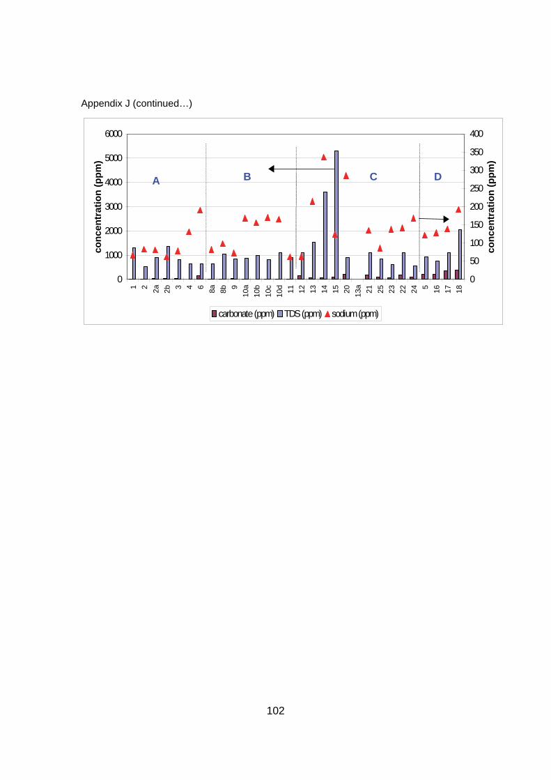
102
Appendix J (continued…)
0
1000
2000
3000
4000
5000
60001 2 2a 2b 3 4 6 8a 8b 9
10a
10b
10c
10d
11 12 13 14 15 20 13a
21 25 23 22 24 5 16 17 18
con
cen
trat
ion
(p
pm
)
0
50
100
150
200
250
300
350
400
con
cen
trat
ion
(p
pm
)
carbonate (ppm) TDS (ppm) sodium (ppm)
A B DC

103
Appendix J (continued…)
Third sampling: Beginning of dry season (BDS)
0
1
2
3
4
5
6
7
8
1 2 2a 2b 3 4 6 8a 8b 9
10a
10b
10c
10d
11 12 13 14 15 20 13a
21 25 23 22 24 5 16 17 18
con
cen
trat
ion
(p
pm
)
0
2
4
6
8
10
12
14
16
con
cen
trat
ion
(p
pm
)
fluoride (ppm) copper (ppm) nitrate as nitrogen (ppm)
A B C D
0
50
100
150
200
250
300
350
400
450
1 2 2a
2b 3 4 6 8a
8b 9
10
a
10
b
10
c
10
d
11
12
13
14
15
20
13
a
21
25
23
22
24 5 16
17
18
con
cen
trat
ion
(p
pm
)
0
1000
2000
3000
4000
5000
6000
7000
con
cen
trat
ion
(p
pm
)
carbonate sodium TDS
A B C D
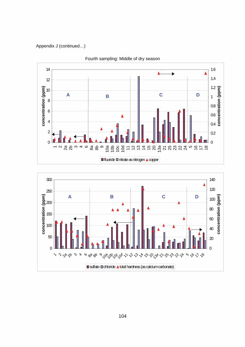
104
Appendix J (continued…)
Fourth sampling: Middle of dry season
0
2
4
6
8
10
12
14
1 2 2a 2b 3 4 6 8a 8b 910
a10
b10
c10
d11 12 13 14 15 20 13
a21 25 23 22 24 5 16 17 18
con
cen
trat
ion
(p
pm
)
0
0.2
0.4
0.6
0.8
1
1.2
1.4
1.6
con
cen
trat
ion
(p
pm
)
fluoride nitrate as nitrogen copper
A B C D
0
50
100
150
200
250
300
1 2 2a 2b 3 4 6 8a 8b 910
a10
b10
c10
d 11 12 13 14 15 20 13a 21 25 23 22 24 5 16 17 18
con
cen
trat
ion
(p
pm
)
0
20
40
60
80
100
120
140
con
cen
trat
ion
(p
pm
)
sulfate chloride total hardness (as calcium carbonate)
A B C D
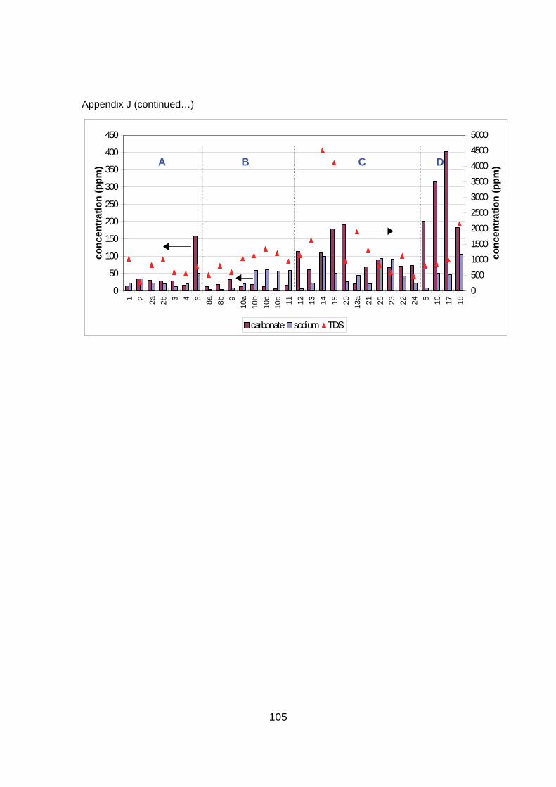
105
Appendix J (continued…)
0
50
100
150
200
250
300
350
400
4501 2 2a 2b 3 4 6 8a 8b 9
10a
10b
10c
10d
11 12 13 14 15 20 13a
21 25 23 22 24 5 16 17 18
con
cen
trat
ion
(p
pm
)
0
500
1000
1500
2000
2500
3000
3500
4000
4500
5000
con
cen
trat
ion
(p
pm
)
carbonate sodium TDS
A B C D

106
Appendix J (continued…)
Averaged values
0
50
100
150
200
250
300
350
400
1 2 2a 2b 3 4 6 8a 8b 9
10a
10b
10c
10d
11 12 13 14 15 20 13a
21 25 23 22 24 5 16 17 18
con
cen
trat
ion
(p
pm
)
0
1000
2000
3000
4000
5000
6000
con
cen
trat
ion
(p
pm
)
carbonate sodium TDS
A B C D
0
20
40
60
80
100
120
140
160
180
1 2 2a
2b 3 4 6 8a
8b 9
10
a
10
b
10
c
10
d
11
12
13
14
15
20
13
a
21
25
23
22
24 5 16
17
18
con
cen
trat
ion
(p
pm
)
0
20
40
60
80
100
120
con
cen
trat
ion
(p
pm
)
sulfates chloride total hardness
A B C D

107
Appendix K Water classification by maximum recorded values of components in the sampled water for the Rustenburg, Klerksdorp and Koster regions
Rustenburg Sampling point
12 13 14 15 20 13a 21 25 23 22 24
Fluoride
Drinking (Health) B G P Y P P P P P P P Drinking (Aesthetic) B B B B B B B B B B B Food preparation B G P Y P P P P P P P Bathing B B B B B B B B B B B Laundry B B B B B B B B B B B
Nitrate
Drinking Health B Y G B G B G G B B B Drinking Aesthetic B B B B B B B B B B B Food preparation B Y G B G B G G B B B Bathing B G B B B B B B B B B Laundry B B B B B B B B B B B
Sulfate
Drinking Health B B Y G G B B B B B B Drinking Aesthetic B B Y G G B B B B B B Food preparation B B Y G G B B B B B B Bathing B B B B B B B B B B B Laundry B B Y G G B B B B B B
Rustenburg
Sampling point
12 13 14 15 20 13a 21 25 23 22 24
pH
Drinking (Health) B B B B B B B B B B B Drinking (Aesthetic) B B B B B B B B B B B Food preparation B B B B B B B B B B B Bathing B B B B B B B B B B B Laundry B B B B B B B B B B B
Chloride
Drinking (Health) G B B B B B B B B B B Drinking (Aesthetic) G B B B B B B B B B B Food preparation G B B B B B B B B B B Bathing B B B B B B B B B B B Laundry B B B B B B B B B B B
Sodium
Drinking (Health) B Y Y G Y B G B G G G Drinking (Aesthetic) B Y Y G Y B G B G G G Food preparation B Y Y G Y B G B G G G Bathing B B B B B B B B B B B Laundry B B B B B B B B B B B
Total hardness
Drinking (Health) B B B B B B B B B B B Drinking (Aesthetic) B B B B B B B B B B B Food preparation B B G B B B B B B B B Bathing G G G G G G G B G G G Laundry B B G B B B B Y G B B
Copper
Drinking (Health) B B B B B Y B B B B B Drinking (Aesthetic) G G B B B Y B B B G B Food preparation G G B B B Y B B B G B Bathing B B B B B Y B B B B B Laundry G G B B B Y B B B G B
TDS
Drinking (Health) Y Y P P G Y Y G G Y G Drinking (Aesthetic) Y Y P P G Y Y G G Y G Food preparation Y Y P P G Y Y G G Y G Bathing B B Y Y B B B B B B B Laundry G G R R B G G G G G B

108
Appendix K (continued…)
Rustenburg Sampling point
12 13 14 15 20 13a 21 25 23 22 24
pH
Drinking (Health) B B B B B B B B B B B Drinking (Aesthetic) B B B B B B B B B B B Food preparation B B B B B B B B B B B Bathing B B B B B B B B B B B Laundry B B B B B B B B B B B
Chloride
Drinking (Health) G B B B B B B B B B B Drinking (Aesthetic) G B B B B B B B B B B Food preparation G B B B B B B B B B B Bathing B B B B B B B B B B B Laundry B B B B B B B B B B B
Sodium
Drinking (Health) B Y Y G Y B G B G G G Drinking (Aesthetic) B Y Y G Y B G B G G G Food preparation B Y Y G Y B G B G G G Bathing B B B B B B B B B B B Laundry B B B B B B B B B B B
Total hardness
Drinking (Health) B B B B B B B B B B B Drinking (Aesthetic) B B B B B B B B B B B Food preparation B B G B B B B B B B B Bathing G G G G G G G B G G G Laundry B B G B B B B Y G B B
Copper
Drinking (Health) B B B B B Y B B B B B Drinking (Aesthetic) G G B B B Y B B B G B Food preparation G G B B B Y B B B G B Bathing B B B B B Y B B B B B Laundry G G B B B Y B B B G B
TDS
Drinking (Health) Y Y P P G Y Y G G Y G Drinking (Aesthetic) Y Y P P G Y Y G G Y G Food preparation Y Y P P G Y Y G G Y G Bathing B B Y Y B B B B B B B Laundry G G R R B G G G G G B

109
Appendix K (continued…)
Klerksdorp and Koster Sampling point
Klerksdorp Koster 1 2 2a 2b 3 4 6 8a 8b 9 10a 10b 10c 10d
pH
Drinking (Health) B B B B B B B B B B B B B B Drinking (Aesthetic) B B B B B B B B B B B B B B Food preparation B B B B B B B B B B B B B B Bathing B B B B B B B B B B B B B B Laundry B B B B B B B B B B B B B B
Chloride
Drinking (Health) B B B B B B B B B B B B B B Drinking (Aesthetic) B B B B B B B B B B B B B B Food preparation B B B B B B B B B B B B B B Bathing B B B B B B B B B B B B B B Laundry B B B B B B B B B B B B B B
Sodium
Drinking (Health) G B B B B G Y B B B G G G G Drinking (Aesthetic) G B B B B G Y B B B G G G G Food preparation G B B B B G Y B B B G G G G Bathing B B B B B B B B B B B B B B Laundry B B B B B B B B B B B B B B
Total hardness
Drinking (Health) B B B B B B B B B B B B B B Drinking (Aesthetic) B B B B B B B B B B B B B B Food preparation B B B B B B B B B B B B B B Bathing G G G G G G G G G G G G G G Laundry B B G G G G B G G B B B B B
Copper
Drinking (Health) B B B B B B B B Y Y Y B B B Drinking (Aesthetic) B B B B B B B B Y Y Y G G B Food preparation B B B B B B B B Y Y Y G G B Bathing B B B B B B B B Y Y Y B B B Laundry B B B B B B B B Y Y Y G G B
Fluoride
Drinking (Health) Y G G G B R R G B B G Y Y Y Drinking (Aesthetic) B B B B B B B B B B B B B B Food preparation Y G G G B R R G B B G Y Y Y Bathing B B B B B B B B B B B B B B Laundry B B B B B B B B B B B B B B
Nitrate
Drinking (Health) Y G G B B G B B B B B B B B Drinking (Aesthetic) B B B B B B B B B B B B B B Food preparation Y G G B B G B B B B B B B B Bathing G B B B B B B B B B B B B B Laundry B B B B B B B B B B B B B B
Sulfate
Drinking (Health) B B B B B B G B B B B B B B Drinking (Aesthetic) B B B B B B G B B B B B B B Food preparation B B B B B B G B B B B B B B Bathing B B B B B B B B B B B B B B Laundry B B B B B B G B B B B B B B
TDS
Drinking (Health) Y G Y R G G Y G Y G Y Y Y Y Drinking (Aesthetic) Y G Y R G G Y G Y G Y Y Y Y Food preparation Y G Y R G G Y G Y G Y Y Y Y Bathing B B B G B B B B B B B B B B Laundry G B G Y B B G B G B G G G G

110
Appendix L Water classification based on average recorded values over four sampling opportunities for the Rustenburg, Klerksdorp and Koster regions
Rustenburg Sampling point
12 13 14 15 20 13a 21 25 23 22 24
Fluoride
Drinking (Health) B G R B R R P P P P R Drinking (Aesthetic) B B B B B B B B B B B Food preparation B G R B R R P P P P R Bathing B B B B B B B B B B B Laundry B B B B B B B B B B B
Nitrate
Drinking (Health) B Y B B B B B B B B B Drinking (Aesthetic) B B B B B B B B B B B Food preparation B Y B B B B B B B B B Bathing B G B B B B B B B B B Laundry B B B B B B B B B B B
Sulfate
Drinking (Health) B B B B B B B B B B B Drinking (Aesthetic) B B B B B B B B B B B Food preparation B B B B B B B B B B B Bathing B B B B B B B B B B B Laundry B B B B B B B B B B B
Rustenburg
Average values Sampling point12 13 14 15 20 13a 21 25 23 22 24
pH
Drinking (Health) B B B B B B B B B B B Drinking (Aesthetic) B B B B B B B B B B B Food preparation B B B B B B B B B B B Bathing B B B B B B B B B B B Laundry B B B B B B B B B B B
Chloride
Drinking (Health) B B B B B B B B B B B Drinking (Aesthetic) B B B B B B B B B B B Food preparation B B B B B B B B B B B Bathing B B B B B B B B B B B Laundry B B B B B B B B B B B
Sodium
Drinking (Health) B G Y Y B B B B G B B Drinking (Aesthetic) B G Y Y B B B B G B B Food preparation B G Y Y B B B B G B B Bathing B B B B B B B B B B B Laundry B B B B B B B B B B B
Total hardness
Drinking (Health) B B B B B B B B B B B Drinking (Aesthetic) B B B B B B B B B B B Food preparation B B B B B B B B B B B Bathing G G G G G G G B G G G Laundry G B B B G G G Y G G G
Copper
Drinking (Health) B B B B B B B B B B B Drinking (Aesthetic) B B B B B G B B B B B Food preparation B B B B B G B B B B B Bathing B B B B B B B B B B B Laundry B B B B B G B B B B B
TDS
Drinking (Health) Y Y P P G Y Y G G Y G Drinking (Aesthetic) Y Y P P G Y Y G G Y G Food preparation Y Y P P G Y Y G G Y G Bathing B B Y Y B B B B B B B Laundry G G R R B G G B B G B

111
Appendix L (continued…)
Rustenburg
Sampling point12 13 14 15 20 13a 21 25 23 22 24
pH
Drinking (Health) B B B B B B B B B B B Drinking (Aesthetic) B B B B B B B B B B B Food preparation B B B B B B B B B B B Bathing B B B B B B B B B B B Laundry B B B B B B B B B B B
Chloride
Drinking (Health) B B B B B B B B B B B Drinking (Aesthetic) B B B B B B B B B B B Food preparation B B B B B B B B B B B Bathing B B B B B B B B B B B Laundry B B B B B B B B B B B
Sodium
Drinking (Health) B G Y Y B B B B G B B Drinking (Aesthetic) B G Y Y B B B B G B B Food preparation B G Y Y B B B B G B B Bathing B B B B B B B B B B B Laundry B B B B B B B B B B B
Total hardness
Drinking (Health) B B B B B B B B B B B Drinking (Aesthetic) B B B B B B B B B B B Food preparation B B B B B B B B B B B Bathing G G G G G G G B G G G Laundry G B B B G G G Y G G G
Copper
Drinking (Health) B B B B B B B B B B B Drinking (Aesthetic) B B B B B G B B B B B Food preparation B B B B B G B B B B B Bathing B B B B B B B B B B B Laundry B B B B B G B B B B B
TDS
Drinking (Health) Y Y P P G Y Y G G Y G Drinking (Aesthetic) Y Y P P G Y Y G G Y G Food preparation Y Y P P G Y Y G G Y G Bathing B B Y Y B B B B B B B Laundry G G R R B G G B B G B
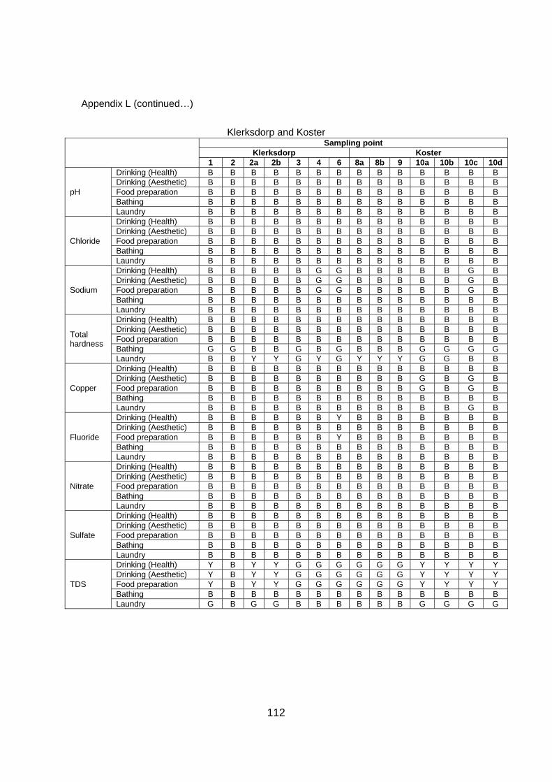
112
Appendix L (continued…)
Klerksdorp and Koster
Sampling pointKlerksdorp Koster
1 2 2a 2b 3 4 6 8a 8b 9 10a 10b 10c 10d
pH
Drinking (Health) B B B B B B B B B B B B B B Drinking (Aesthetic) B B B B B B B B B B B B B B Food preparation B B B B B B B B B B B B B B Bathing B B B B B B B B B B B B B B Laundry B B B B B B B B B B B B B B
Chloride
Drinking (Health) B B B B B B B B B B B B B B Drinking (Aesthetic) B B B B B B B B B B B B B B Food preparation B B B B B B B B B B B B B B Bathing B B B B B B B B B B B B B B Laundry B B B B B B B B B B B B B B
Sodium
Drinking (Health) B B B B B G G B B B B B G B Drinking (Aesthetic) B B B B B G G B B B B B G B Food preparation B B B B B G G B B B B B G B Bathing B B B B B B B B B B B B B B Laundry B B B B B B B B B B B B B B
Total hardness
Drinking (Health) B B B B B B B B B B B B B B Drinking (Aesthetic) B B B B B B B B B B B B B B Food preparation B B B B B B B B B B B B B B Bathing G G B B G B G B B B G G G G Laundry B B Y Y G Y G Y Y Y G G B B
Copper
Drinking (Health) B B B B B B B B B B B B B B Drinking (Aesthetic) B B B B B B B B B B G B G B Food preparation B B B B B B B B B B G B G B Bathing B B B B B B B B B B B B B B Laundry B B B B B B B B B B B B G B
Fluoride
Drinking (Health) B B B B B B Y B B B B B B B Drinking (Aesthetic) B B B B B B B B B B B B B B Food preparation B B B B B B Y B B B B B B B Bathing B B B B B B B B B B B B B B Laundry B B B B B B B B B B B B B B
Nitrate
Drinking (Health) B B B B B B B B B B B B B B Drinking (Aesthetic) B B B B B B B B B B B B B B Food preparation B B B B B B B B B B B B B B Bathing B B B B B B B B B B B B B B Laundry B B B B B B B B B B B B B B
Sulfate
Drinking (Health) B B B B B B B B B B B B B B Drinking (Aesthetic) B B B B B B B B B B B B B B Food preparation B B B B B B B B B B B B B B Bathing B B B B B B B B B B B B B B Laundry B B B B B B B B B B B B B B
TDS
Drinking (Health) Y B Y Y G G G G G G Y Y Y Y Drinking (Aesthetic) Y B Y Y G G G G G G Y Y Y Y Food preparation Y B Y Y G G G G G G Y Y Y Y Bathing B B B B B B B B B B B B B B Laundry G B G G B B B B B B G G G G
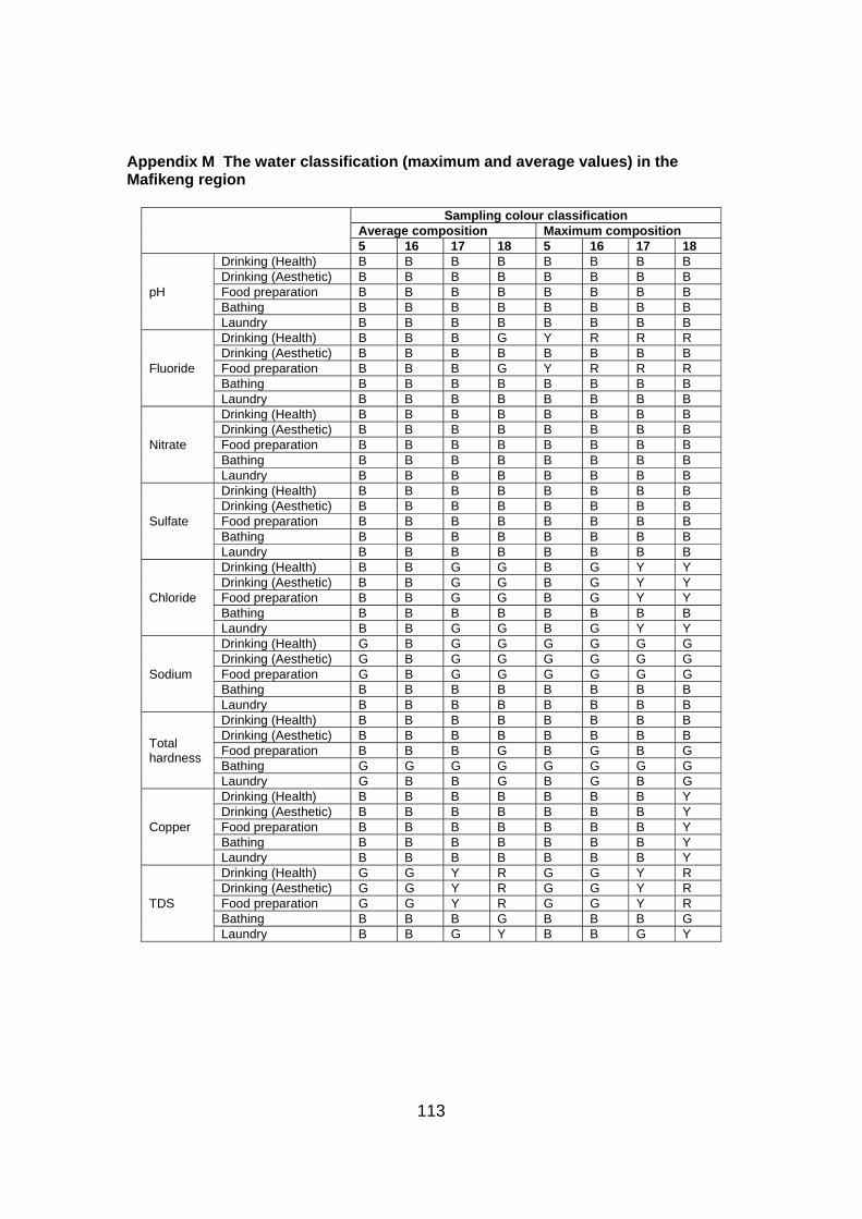
113
Appendix M The water classification (maximum and average values) in the Mafikeng region
Sampling colour classification Average composition Maximum composition 5 16 17 18 5 16 17 18
pH
Drinking (Health) B B B B B B B B Drinking (Aesthetic) B B B B B B B B Food preparation B B B B B B B B Bathing B B B B B B B B Laundry B B B B B B B B
Fluoride
Drinking (Health) B B B G Y R R R Drinking (Aesthetic) B B B B B B B B Food preparation B B B G Y R R R Bathing B B B B B B B B Laundry B B B B B B B B
Nitrate
Drinking (Health) B B B B B B B B Drinking (Aesthetic) B B B B B B B B Food preparation B B B B B B B B Bathing B B B B B B B B Laundry B B B B B B B B
Sulfate
Drinking (Health) B B B B B B B B Drinking (Aesthetic) B B B B B B B B Food preparation B B B B B B B B Bathing B B B B B B B B Laundry B B B B B B B B
Chloride
Drinking (Health) B B G G B G Y Y Drinking (Aesthetic) B B G G B G Y Y Food preparation B B G G B G Y Y Bathing B B B B B B B B Laundry B B G G B G Y Y
Sodium
Drinking (Health) G B G G G G G G Drinking (Aesthetic) G B G G G G G G Food preparation G B G G G G G G Bathing B B B B B B B B Laundry B B B B B B B B
Total hardness
Drinking (Health) B B B B B B B B Drinking (Aesthetic) B B B B B B B B Food preparation B B B G B G B G Bathing G G G G G G G G Laundry G B B G B G B G
Copper
Drinking (Health) B B B B B B B Y Drinking (Aesthetic) B B B B B B B Y Food preparation B B B B B B B Y Bathing B B B B B B B Y Laundry B B B B B B B Y
TDS
Drinking (Health) G G Y R G G Y R Drinking (Aesthetic) G G Y R G G Y R Food preparation G G Y R G G Y R Bathing B B B G B B B G Laundry B B G Y B B G Y

114
Appendix N General performance of NF membranes
Membrane performance D11 D12 NF70 NF90 TFC-S TFC-
SR TFC-ULP
CTC-1
Lero
me
Fluoride - - - - + + - - + + - - + + - - Nitrate - - + + + - - - - - + - - Overall - - - - + + - - - - - + + - - Sulfate + + + + + + + + + + + + + + + + Calcium - - + - - + + - - + + - - - - Magnesium - - - - - - - - - - - - - Overall - + - + + + + - + + + - - -
Membrane performance D11 D12 NF70 NF90 TFC-S TFC-
SR TFC-ULP
CTC-1
Kaa
llaa
gte
Fluoride + + - - - - - - - - - + + - - Nitrate - - - - + + + + + - - - - - Overall - - - + - - - - - - - - - Sulfate + + + + + + + + + + + + + + + + Calcium + + - - + + + - - - + + - - + Magnesium - - - - - - - - - - - - - Overall + - + + + - - + + - + -
Membrane performance D11 D12 NF70 NF90 TFC-S TFC-
SR TFC-ULP
CTC-1
Rhe
nost
erfo
ntei
n Fluoride - - - - - - - + + + - - + - Nitrate - - - - + + - - - - - - - - - Overall - - - - - - - + - - - - - Sulfate + + + + + + + + + + + + + + + + Calcium + + - + + + - - - - + - + + Magnesium - - - - - - - - - - - - - - - - Overall + + - + - + - + + - + +
Membrane performance D11 D12 NF70 NF90 TFC-S TFC-
SR TFC-ULP
CTC-1
Rie
tvle
i
Fluoride - - - - - - - - - - - - - - - - Nitrate - - - + - - - - - - - - - Overall - - - - - - - - - - - - - - - Sulfate + + + + + + + + + + + + + + + + Calcium + + - + - + - + - + - + + + - Magnesium - - - - + + - - - - - - - + - Overall + - + + + - + + + + +
Membrane performance D11 D12 NF70 NF90 TFC-S TFC-
SR TFC-ULP
CTC-1
Vaa
l Riv
er
Fluoride - - - - + + - - - - - - - - - - Nitrate - - + - - + - - + + - Overall - - - + + - - - - - - - - Sulfate + + + + + + + + + + + + + + + + Calcium - - - - + + + + - - + + - - - Magnesium - - - - - - - + - - - - - - Overall - - - - + + + - + - + + + - -
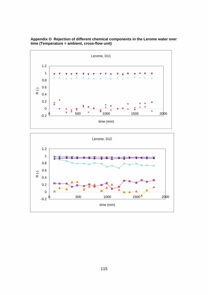
115
Appendix O Rejection of different chemical components in the Lerome water over time (Temperature = ambient, cross-flow unit)
Lerome, D11
-0.2
0
0.2
0.4
0.6
0.8
1
1.2
0 500 1000 1500 2000
time (min)
R (
-)
Lerome, D12
-0.2
0
0.2
0.4
0.6
0.8
1
1.2
0 500 1000 1500 2000
time (min)
R (
-)
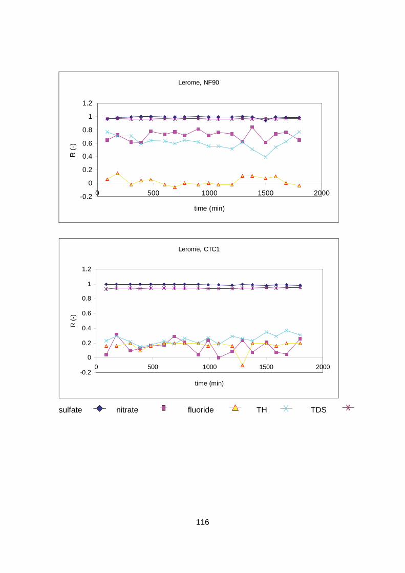
116
Lerome, NF90
-0.2
0
0.2
0.4
0.6
0.8
1
1.2
0 500 1000 1500 2000
time (min)
R (
-)
Lerome, CTC1
-0.2
0
0.2
0.4
0.6
0.8
1
1.2
0 500 1000 1500 2000
time (min)
R (
-)
sulfate nitrate fluoride TH TDS

117
Appendix P Rejection of different chemical components on various membranes in the Ledig water over time (Temperature = ambient, cross-flow unit)
Ledig, D11
-0.2
0
0.2
0.4
0.6
0.8
1
1.2
0 500 1000 1500 2000
time (min)
R (
-)
Ledig, D12
-0.2
0
0.2
0.4
0.6
0.8
1
1.2
0 500 1000 1500 2000
time (min)
R (
-)

118
Ledig, NF90
0
0.2
0.4
0.6
0.8
1
1.2
0 500 1000 1500 2000
time(min)
R(-
)
Ledig, CTC1
0
0.2
0.4
0.6
0.8
1
1.2
0 500 1000 1500 2000
time (min)
R(-
)
sulfate nitrate fluoride TH TDS

119
Appendix Q Rejection of different chemical components on various membranes in the Haaskraal water over time (Temperature = ambient, cross-flow unit)
Haaskraal, D11
0
0.2
0.4
0.6
0.8
1
1.2
0 500 1000 1500 2000
time (min)
R (
-)
Haaskraal, D12
-0.2
0
0.2
0.4
0.6
0.8
1
1.2
0 500 1000 1500 2000
time (min)
R (
-)
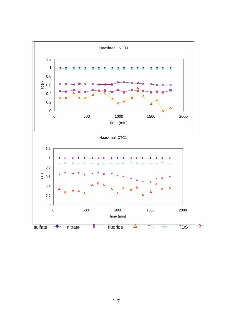
120
Haaskraal, NF90
0
0.2
0.4
0.6
0.8
1
1.2
0 500 1000 1500 2000
time (min)
R (
-)
Haaskraal, CTC1
0
0.2
0.4
0.6
0.8
1
1.2
0 500 1000 1500 2000
time (min)
R (
-)
sulfate nitrate fluoride TH TDS

121
Appendix R Rejection of different chemical components on various membranes in the Vaal River over time (Temperature = ambient, cross-flow unit)
Vaal River, D11
0
0.2
0.4
0.6
0.8
1
1.2
0 500 1000 1500 2000
time (min)
R (
-)
Vaal River, D12
0
0.2
0.4
0.6
0.8
1
1.2
0 500 1000 1500 2000
time (min)
R (
-)
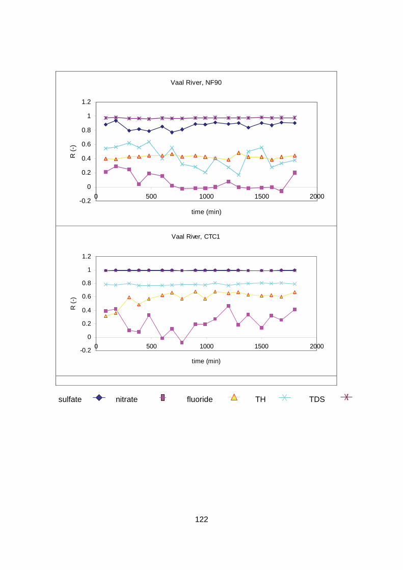
122
Vaal River, NF90
-0.2
0
0.2
0.4
0.6
0.8
1
1.2
0 500 1000 1500 2000
time (min)
R (
-)
Vaal River, CTC1
-0.2
0
0.2
0.4
0.6
0.8
1
1.2
0 500 1000 1500 2000
time (min)
R (
-)
sulfate nitrate fluoride TH TDS

123
Appendix S Membrane performance in rejecting various chemical components from selected sites
Flouride
Lerome
[F]o = 5.78ppm
Ledig
[F]o = 7.23ppm
Haaskraal
[F]o = 0.22ppm
Vaal River
[F]o = 2.71ppm
Brine Product Brine Product Brine Product Brine Product
D11 5.93 5.67 9.14 5.26 0.25 0.15 4.00 1.40
D12 6.36 5.23 9.07 5.33 0.23 0.17 3.81 1.59
NF90 5.17 5.63 9.94 4.46 0.26 0.14 3.83 1.57
CTC1 6.79 4.81 9.43 4.97 6.27 0.13 4.29 1.11
Nitrate
Lerome
[NO3-]o = 1.21ppm
Ledig
[NO3-]o = 1.76ppm
Haaskraal
[NO3-]o = 13.9ppm
Vaal River
[NO3-]o = 1.60ppm
Brine Product Brine Product Brine Product Brine Product
D11 1.25 1.15 2.04 1.56 21.0 6.81 2.21 0.99
D12 1.47 0.93 2.48 1.12 20.1 7.37 2.05 1.15
NF90 2.05 0.35 2.59 1.01 20.4 7.37 1.71 1.49
CTC1 1.38 1.02 2.11 1.49 22.5 5.28 1.97 1.23
Sulfate
Lerome
[SO42-]o = 50ppm
Ledig
[SO42-]o = 20ppm
Haaskraal
[SO42-]o = 70ppm
Vaal River
[SO42-]o = 112ppm
Brine Product Brine Product Brine Product Brine Product
D11 99.0 1.0 38.2 1.8 140 0 219 4.5
D12 96.8 3.2 38.2 1.8 140 0 222 2.2
NF90 99.4 0.7 40.0 0.0 140 0 208 15.7
CTC1 100.0 0.5 38.2 1.8 140 0 223 1.1
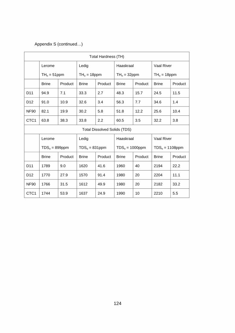
124
Appendix S (continued…)
Total Hardness (TH)
Lerome
THo = 51ppm
Ledig
THo = 18ppm
Haaskraal
THo = 32ppm
Vaal River
THo = 18ppm
Brine Product Brine Product Brine Product Brine Product
D11 94.9 7.1 33.3 2.7 48.3 15.7 24.5 11.5
D12 91.0 10.9 32.6 3.4 56.3 7.7 34.6 1.4
NF90 82.1 19.9 30.2 5.8 51.8 12.2 25.6 10.4
CTC1 63.8 38.3 33.8 2.2 60.5 3.5 32.2 3.8
Total Dissolved Solids (TDS)
Lerome
TDSo = 899ppm
Ledig
TDSo = 831ppm
Haaskraal
TDSo = 1000ppm
Vaal River
TDSo = 1108ppm
Brine Product Brine Product Brine Product Brine Product
D11 1789 9.0 1620 41.6 1960 40 2194 22.2
D12 1770 27.9 1570 91.4 1980 20 2204 11.1
NF90 1766 31.5 1612 49.9 1980 20 2182 33.2
CTC1 1744 53.9 1637 24.9 1990 10 2210 5.5