LD Didactic GmbH . Leyboldstrasse 1 . D-50354 Huerth / Germany . Phone: (02233) 604-0 . Fax: (02233) 604-222 . e-mail: info@ld-didactic.de by LD Didactic GmbH Printed in the Federal Republic of Germany Technical alterations reserved

P3.4.6.1

LD

Physics

Leaflets

Electricity

Electromagnetic induction

Measuring the earth’s magnetic field

Measuring the earth’s mag-netic field with a rotating induc-tion coil (earth inductor)

Objects of the experiment

g Determination of the components of the earth’s magnetic field.

g Determination of the inclination angle of the earth ‘s magnetic field.

Bi

03

05

Principles

When circular induction coil with N turns and an area A = π⋅R2

rotates at a constant angular velocity ω in an homogenous magnetic field B around its diameter d as an axis it is perme-ated by a magnetic flux

)tcos(BNR2 ⋅ω⋅⋅⋅⋅π=Φ (I)

ω: angular velocity

R: radius of the induction coil

N: turns of the induction coil

Equation (I) assumes that the axis of rotation is perpendicular to the magnetic field B. The magnetic field B can be deter-mined from the amplitude of the induced voltage U by

)tsin(BNRdt

dU 2 ⋅ω⋅ω⋅⋅⋅⋅π=

Φ−= (II)

Using the revolution time T = 2⋅π / ω we find for the peak value of the induced AC voltage:

BaBT

RNU ⋅=⋅

⋅⋅⋅=

222ˆ π

(III)

T

RNa

222 ⋅⋅⋅

=π

(IV)

For a rotation of the coil around the z-direction of a Cartesian coordinate system (Fig. 1) the voltage amplitude

2y

2xZ BBaU +⋅= (V)

is induced in the earth’s magnetic field

=

z

y

x

B

B

B

Br

(VI)

For reasons of symmetry the following equations apply for orientations in the x- or y-direction:

2z

2yx BBaU +⋅= (VII)

2x

2zy BBaU +⋅= (VIII)

The components of the earth’s magnetic field can be calcu-lated by resolving the system of equations (V), (VII) and (VIII):

2

2z

2y

2x

xa2

UUUB

⋅

++−= (IX)

2

2z

2y

2x

ya2

UUUB

⋅

+−= (X)

2

2z

2y

2x

za2

UUUB

⋅

−+= (XI)

In particular, we have for the total value of the earth’s mag-netic field:

2

2z

2y

2x2

z2y

2x

a2

UUUBBBB

⋅

++=++= (XII)

P3.4.6.1 - 2 - LD Physics leaflets

LD Didactic GmbH . Leyboldstrasse 1 . D-50354 Huerth / Germany . Phone: (02233) 604-0 . Fax: (02233) 604-222 . e-mail: info@ld-didactic.de by LD Didactic GmbH Printed in the Federal Republic of Germany Technical alterations reserved

The angle of the dip ϑ of the earth’s magnetic field can be obtained by the relation:

2z

2z

2y

2x

2y

2x

z

U2

UUU

BB

Btan

⋅

−+=

+=ϑ (XIII)

This formula is mathematically correct, but due to unavoid-able measurement imprecision the argument of the square root might become negative when the experiment is carried out close to the equator. For a solution see the end of this leaflet.

In this experiment the axis of rotation of the induction coil is aligned in the x-, y- and z-direction of a rectangular coordi-nate system successively. The amplitude of the induced volt-age is measured as function of time with CASSY in each case. From the recorded signals the amplitude and frequency is used to determine the strength and angle of the dip of the earth’s magnetic field.

Fig. 1: Experimental setup with experiment motor (schematically).

Setup

- Place the experiment motor on the corner of the bench like shown in Fig. 1 so that an alignment in three directions (x, y, z) is possible.

- Use two 2 m long twisted connecting leads for the connec-

tion between the µV-box and the induction loop.

Carrying out the experiment

Carrying out the experiment with experiment motor

- Load the CASSY example file “earth magnetic field”. Note: This file is not listed in the CASSY experiment example files. It has to be loaded from the hard disk by using the

button or pressing the function key F3.

- Clear the example data by using the button or pressing the function key F4.

- Set the speed of the experiment motor to zero.

- Switch on the motor carefully and increase gently the speed to approximately 0.3 revolutions per second.

- Guide the twisted connecting leads by hand so that they are wound up by the experiment motor. Ensure that they are not get caught in the chuck while the conductor loop is rotating.

- Start the measurement of the induced voltage as function of time by pressing the function key F9 or using the button

alternatively.

- Note: The measurement stops automatically after 20 s. For details of the measurement parameters press two

times to see the settings in the menu “measuring pa-rameter”.

- Make sure that the motor is switched off after the meas-urement is finished. Reverse the experiment motor’s direc-tion and stop the motor in good time.

- Change the axis of rotation to the x-direction and repeat the measurement for the same angular velocity.

- Finally turn the experiment motor by 90° degree to meas-ure the induction voltage as function of time for the y-direction as axis of rotation.

- Measure the diameter d of the induction coil.

Carrying out the experiment without experiment motor

- Load the CASSY example file “earth magnetic field”. Note: This file is not listed in the CASSY experiment example files. It has to be loaded from the hard disk by using the

button or pressing the function key F3.

- Clear the example data by using the button or pressing the function key F4.

- Start the measurement of the induced voltage as function of time by pressing the function key F9 or using the button

alternatively.

- Rotate the induction coil manually around the z-direction.

- Note: The measurement stops automatically after 20 s. For details of the measurement parameters press two

times to see the settings in the menu “measuring pa-rameter”.

- Repeat the measurement for the rotation about the y- and x-direction.

Apparatus

1 Pair of Helmholtz coils.................................. 555 604 1 Sensor CASSY............................................. 524 010USB 1 µV-box.......................................................... 524 040 1 CASSY Lab.................................................. 524 200 1 Connecting lead Ø 2,5 mm

2, 200 cm, red .... 501 35

1 Connecting lead Ø 2,5 mm2, 200 cm, blue... 501 36

Additionally recommended:

1 Experiment motor......................................... 347 35 1 Control unit for experiment motor................. 347 36

Additionally required:

1 PC with Windows 2000/XP/Vista

LD Physics leaflets - 3 - P3.4.6.1

LD Didactic GmbH . Leyboldstrasse 1 . D-50354 Huerth / Germany . Phone: (02233) 604-0 . Fax: (02233) 604-222 . e-mail: info@ld-didactic.de by LD Didactic GmbH Printed in the Federal Republic of Germany Technical alterations reserved

Measuring example

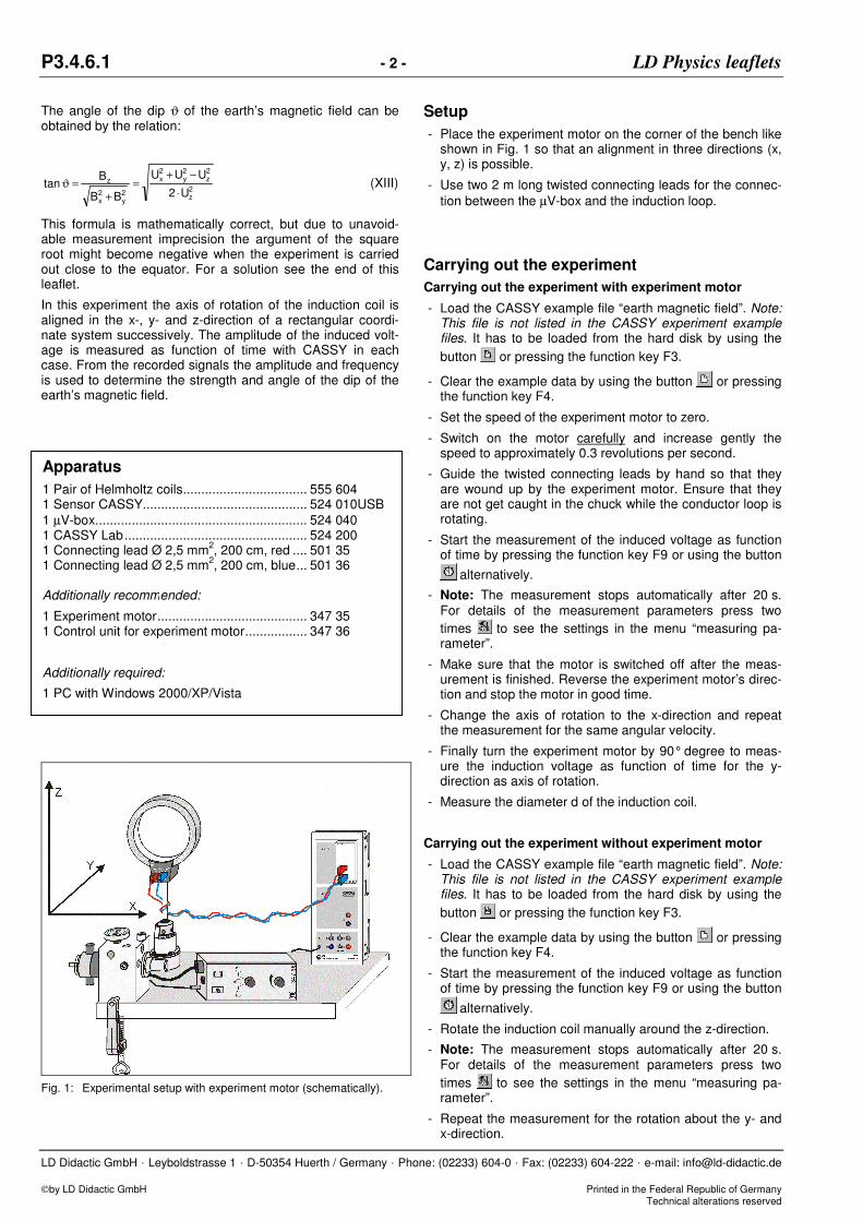
In Fig. 2, as an example, the voltage curve for the rotation around the x-axis is shown. For the result around the rotation around the y- and z-axis see Fig. 5. and Fig. 6.

Fig. 2: Induced voltage Ux as function of time (z-direction = axis of rotation).

Evaluation and results

To determine the components of the earth’s magnetic field the amplitude and frequency has to be determined. There are several ways to determine the frequency.

Method 1

- Click right mouse button in the display and choose “Set Marker/Measure Difference” (Fig. 3).

- Click e.g. on a zero voltage position and repeat this at the position after the period T.

- Alt T allows you to display the result of the status line in the display (Fig. 3).

Fig. 3: Determination of the Frequency (Method 1). Compare Fig. 4 and Fig 5.

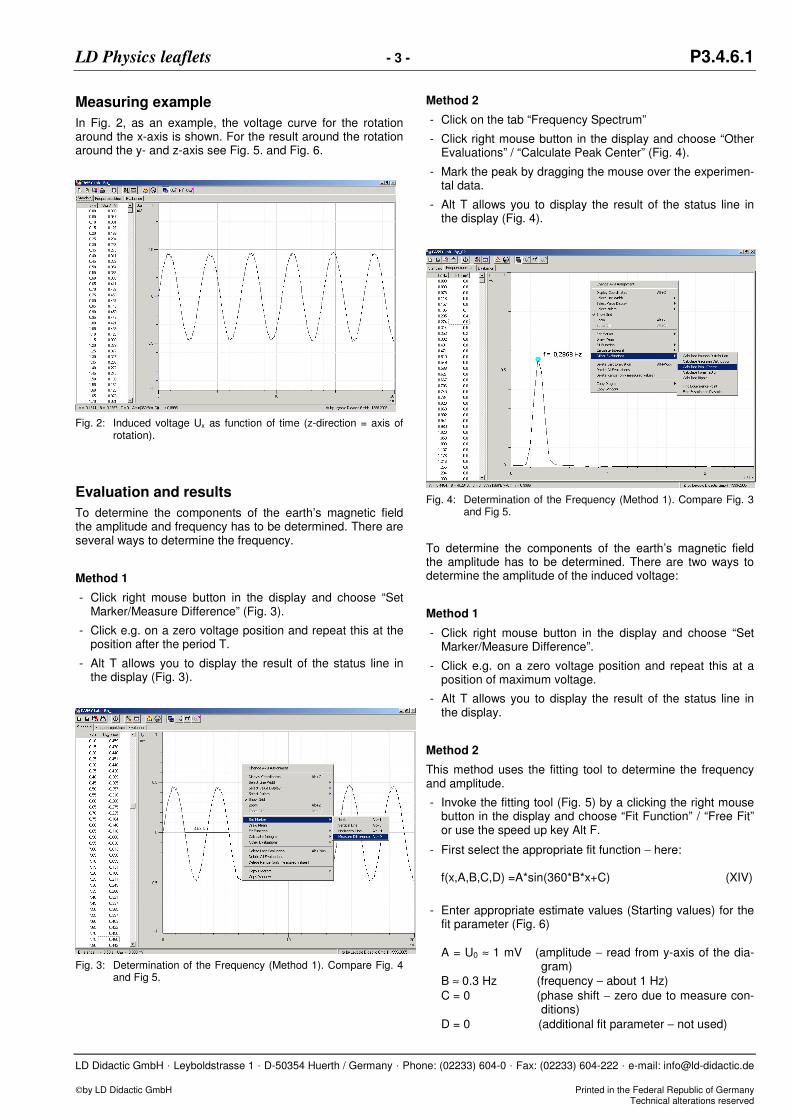
Method 2

- Click on the tab “Frequency Spectrum”

- Click right mouse button in the display and choose “Other Evaluations” / “Calculate Peak Center” (Fig. 4).

- Mark the peak by dragging the mouse over the experimen-tal data.

- Alt T allows you to display the result of the status line in the display (Fig. 4).

Fig. 4: Determination of the Frequency (Method 1). Compare Fig. 3 and Fig 5.

To determine the components of the earth’s magnetic field the amplitude has to be determined. There are two ways to determine the amplitude of the induced voltage:

Method 1

- Click right mouse button in the display and choose “Set Marker/Measure Difference”.

- Click e.g. on a zero voltage position and repeat this at a position of maximum voltage.

- Alt T allows you to display the result of the status line in the display.

Method 2

This method uses the fitting tool to determine the frequency and amplitude.

- Invoke the fitting tool (Fig. 5) by a clicking the right mouse button in the display and choose “Fit Function” / “Free Fit” or use the speed up key Alt F.

- First select the appropriate fit function − here: f(x,A,B,C,D) =A*sin(360*B*x+C) (XIV)

- Enter appropriate estimate values (Starting values) for the fit parameter (Fig. 6) A = U0 ≈ 1 mV (amplitude − read from y-axis of the dia- gram) B ≈ 0.3 Hz (frequency − about 1 Hz)

C = 0 (phase shift − zero due to measure con- ditions)

D = 0 (additional fit parameter − not used)

P3.4.6.1 - 4 - LD Physics leaflets

LD Didactic GmbH . Leyboldstrasse 1 . D-50354 Huerth / Germany . Phone: (02233) 604-0 . Fax: (02233) 604-222 . e-mail: info@ld-didactic.de by LD Didactic GmbH Printed in the Federal Republic of Germany Technical alterations reserved

- Select “Display result automatically as a new channel”

- Continue with the button “Continue with Range Marking”

- Alt T allows you to display the result of the fit quickly in the display.

Fig. 5: Induced voltage Uy (black line) as function of time (y-direction = axis of rotation). The red line corresponds to a fit according to the parameter listed below the voltage curve. Note: The fitting tool can be invoked by a clicking the right mouse button in the display and choose “Fit Function” / “Free Fit”.

Fig. 5. and 6 shows a fit to the measured voltage values. Within the error limit the verifies nicely the sinusoidal form. For further data evaluation tools of CASSY Lab see supple-mentary information.

Fig. 6: Induced voltage Uz (black line) as function of time (z-direction = axis of rotation). The red line corresponds to a fit according to the parameter listed below the voltage curve. Note: The fitting tool can be invoked by the speed up key ”Alt-F”.

The result of the fit for the three different axes of rotation are summarized in the following table:

Table 1: Components of the induced voltage obtained by the fit of equation (XIV) to the experimental data. The period corresponds to the mean average over the axes of rotation.

mV

Ux mV

Uy mV

Uz s

T

0.47 0.45 0.13 3.51

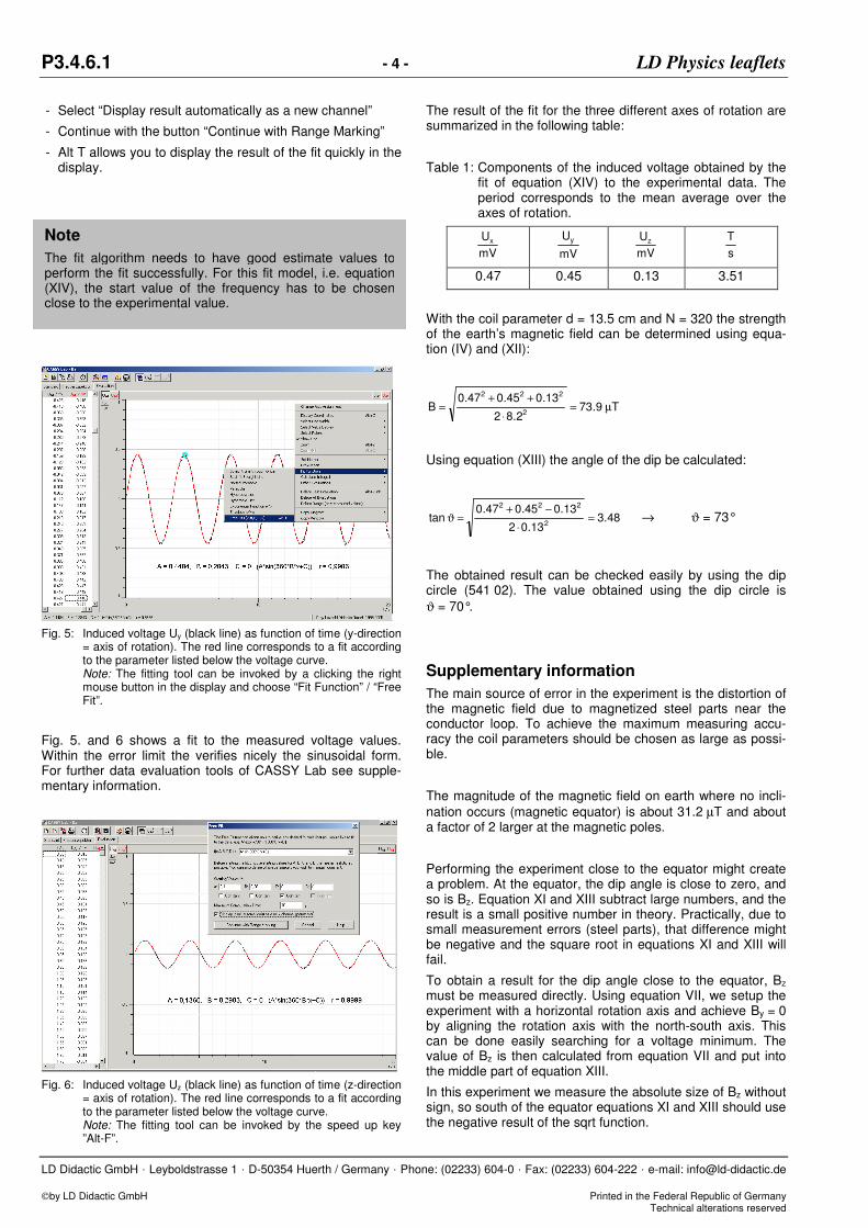
With the coil parameter d = 13.5 cm and N = 320 the strength of the earth’s magnetic field can be determined using equa-tion (IV) and (XII):

T9.732.82

13.045.047.0B

2

222

µ=⋅

++=

Using equation (XIII) the angle of the dip be calculated:

48.313.02

13.045.047.0tan

2

222

=⋅

−+=ϑ → ϑ = 73°

The obtained result can be checked easily by using the dip circle (541 02). The value obtained using the dip circle is

ϑ = 70°.

Supplementary information

The main source of error in the experiment is the distortion of the magnetic field due to magnetized steel parts near the conductor loop. To achieve the maximum measuring accu-racy the coil parameters should be chosen as large as possi-ble.

The magnitude of the magnetic field on earth where no incli-nation occurs (magnetic equator) is about 31.2 µT and about a factor of 2 larger at the magnetic poles.

Performing the experiment close to the equator might create a problem. At the equator, the dip angle is close to zero, and so is Bz. Equation XI and XIII subtract large numbers, and the result is a small positive number in theory. Practically, due to small measurement errors (steel parts), that difference might be negative and the square root in equations XI and XIII will fail.

To obtain a result for the dip angle close to the equator, Bz must be measured directly. Using equation VII, we setup the experiment with a horizontal rotation axis and achieve By = 0 by aligning the rotation axis with the north-south axis. This can be done easily searching for a voltage minimum. The value of Bz is then calculated from equation VII and put into the middle part of equation XIII.

In this experiment we measure the absolute size of Bz without sign, so south of the equator equations XI and XIII should use the negative result of the sqrt function.

Note

The fit algorithm needs to have good estimate values to perform the fit successfully. For this fit model, i.e. equation (XIV), the start value of the frequency has to be chosen close to the experimental value.