Decentralized College Admissions

Yeon-Koo Che and Youngwoo Koh∗

June 24, 2015

Abstract

We study decentralized college admissions with uncertain student preferences. Col-

leges strategically admit students likely to be overlooked by competitors. Highly ranked

students may receive fewer admissions or have a higher chance of receiving no ad-

missions than those ranked below. When students’ attributes are multidimensional,

colleges avoid head-on competition by placing excessive weight on school-specific at-

tributes such as essays. Restricting the number of applications or wait-listing allevi-

ates enrollment uncertainty, but the outcomes are inefficient and unfair. A centralized

matching via Gale and Shapley’s deferred acceptance algorithm attains efficiency and

fairness but may make some colleges worse off than under decentralized matching.

1 Introduction

Centralized matching has gained prominence in economic theory and practice, spurred by

successful applications such as medical residency matching and public school choice. Yet,

many matching markets remain decentralized; college and graduate school admissions are

notable examples. It is often suggested that these markets do not operate well and will

∗Che: Columbia University, yeonkooche@gmail.com; Koh: Hanyang University, young-woo.koh@gmail.com. We have benefitted from comments made by Ethan Che, Prajit Dutta, GlennEllison, Drew Fudenberg, Takakazu Honryo, Navin Kartik, Jinwoo Kim, Fuhito Kojima, Jian Lee, JonathanLevin, Greg Lewis, Qingmin Liu, Janet Lu, Yusuke Narita, Parag Pathak, Mike Peters, Brian Rogers, AlRoth, Xingye Wu, and seminar participants at Chung-Ang Universiy, Harvard-MIT Theory Workshop,Korea University, NYU-IO Days Conference, Seoul National University, Sogang Univerisy, StanfordUniversity, Washington University, Yonsei Universiy, Asian Meeting of the Econometric Society, KoreaEconomic Association Conference, North America Summer Meeting of the Econometric Society, Meeting ofthe Society for Social Choice, and SAET Conference. Che acknowledges the financial support from NationalScience Foundation (NSF1260937) and from the National Research Foundation in Korea through its GlobalResearch Network Grant (NRF-2013S1A2A2035408). Koh gratefully acknowledges funding from HanyangUniversity (HY-2013-N).

1

therefore benefit from improved coordination or complete centralization,1 but it is not well

understood why they remain decentralized and what welfare benefits would be gained by

improved coordination. At least part of the problem is the lack of an analytical grasp of

decentralized matching markets. A seminal work by Roth and Xing (1997) attributes the

problems of such markets to “congestion”—participants are not allowed to make enough

offers and acceptances to clear the market. But, the equilibrium and welfare implications of

congestion remain poorly understood. Indeed, economists have yet to develop a workhorse

model of decentralized matching that can serve as a useful benchmark for comparison with

a centralized system.

The current paper develops an analytical framework for understanding decentralized

matching markets in the context of college admissions. College admissions in countries such

as Japan, Korea and the US are organized similarly to decentralized labor markets: colleges

make exploding and binding admission offers to applicants, and the admitted students ac-

cept or reject the offers, often within a short window of time. This process provides little

opportunity for colleges to learn students’ preferences and adjust their admissions decisions

accordingly. Consequently, they often end up enrolling too many or too few students rela-

tive to their capacities. For instance, 1,415 freshmen accepted Yale’s invitation to join its

incoming class in 1995-96, although the university had aimed for a class of 1,335. In the

same year, Princeton also reported 1,100 entering students, the largest number in its history.

Princeton had to set up mobile homes in fields and build new dorms to accommodate the

students (Avery, Fairbanks, and Zeckhauser, 2003).

Controlling yield is particularly challenging for colleges in Korea, since students apply

to a department, instead of a college, and each department faces a relatively rigid and low

quota. A department that exceeds a pre-specified capacity is subject to a rather harsh

penalty by the government in the form of a sharply reduced capacities in the subsequent

year. The challenge is not much easier for US counterparts. Due to an explosion of the

number of applications,2 the average yield rate of four-year colleges in the US has declined

significantly over the past decade, from 49% in 2001 to 38% in 2011 (National Association

for College Admission Counseling, 2012, NACAC hereafter). The declining rates resulted

in increased uncertainty for colleges—a main theme in the NACAC (2012) report on the

1Coles et al. (2010) provide survey evidence that in the market for new Ph.D. economists, introduction ofa signaling service and a formalized secondary market facilitates matches by improving coordination amongparticipants. Abdulkadiroglu, Agarwal, and Pathak (2015) find the switch in 2002 from a decentralizedmatching mechanism to a centralized one based on DA resulted in a significant gain in utilitarian welfare forapplicants in the New York City Public High School assignment. See also Che (2013) for a further discussionon improving coordination in college admissions.

2The average number of applications per institution increased 60% between 2002 and 2011, and 79% ofFall 2011 freshmen applied to three or more colleges, with 29% of them submitting seven or more applications(NACAC, 2012).

2

current state of US college admissions.3

Importantly, the enrollment uncertainty a college faces depends on the admissions deci-

sions made by other colleges. A student admitted by a college poses a greater uncertainty

for its enrollment when the student is also admitted by other colleges, since her enrollment

depends on the student’s (unknown) preference. This interdependent nature of uncertainty

introduces a strategic interaction among colleges in their admissions decisions. In this paper,

we develop a model that captures this feature.

In our model, there are two colleges, each with limited capacity, and a unit mass of

students. Colleges may value two attributes of a student: a “score” (e.g., high school grade

point average (GPA) or Scholastic Aptitude Test (SAT) scores) that is common to all colleges

and a “fit” (e.g., college-specific essays/exams or extracurricular activities) that is college-

specific and statistically independent across colleges. Students apply to colleges at no cost.

Colleges rank students according to their “score” and “fit” but they do not observe students’

preferences. This uncertainty takes an aggregate form: the mass of students preferring one

college over the other varies with unknown states of nature. Each college incurs a constant

per-student cost for enrollment exceeding its capacity. Our model involves a simple time-line:

Initially, students simultaneously apply to colleges. Each college observes only the scores and

fit of those students who apply to it. Then, the two colleges simultaneously offer admissions

to sets of students. Finally, students decide on which offer (if any) to accept.

Given that application is costless, students have a (weakly) dominant strategy of applying

to both colleges. Hence, the focus of the analysis is the colleges’ admissions decisions. Our

main finding is that colleges respond to congestion strategically by employing measures that

would avoid head-on competition. Specifically, when the colleges do not value fit significantly,

they may strategically favor students with relatively low scores, for such students are likely

to be overlooked by competitors. Consequently, students with higher scores may receive

admissions from fewer colleges or they may suffer from a higher chance of not being admitted

by any (i.e., “falling through the cracks”), compared to students with lower scores. When

colleges value both score and fit, they avoid head-on competition by biasing their admissions

in favor of those who rank highly in fit against those who rank highly in scores. The outcome

of the equilibrium in both cases is inefficient since at least some colleges leave their seats

unfilled despite there being some unmatched students that the college would have been happy

to admit. Strategic targeting and biased admissions make the outcome also unfair, in the

3 Its preface reads: “A theme that is reflected throughout this report is uncertainty—uncertainty forcolleges, high schools, students and families. Amid an historically large number of students flowing throughthe college application process, we have witnessed unparalleled uncertainty for both students and colleges.”(page 3 of NACAC (2012)). Jennifer Delahunty, dean of admissions and financial aid at Kenyon Collegein Ohio, described the college’s challenge as follows: “Trying to hit those numbers is like trying to hit hottub when you are skydiving 30,000 feet. I’m going to go to church every day in April” (“In Shifting Era ofAdmissions, Colleges Sweat,” by Kate Zernike, New York Times, March 8, 2009).

3

sense of creating “justified envy”: a mass of students are unable to enroll at their favorite

college even though the college enrolls students it ranks below them.

In practice, colleges employ additional measures to cope with congestion. One is to

restrict the number of applications a student can submit, as practiced by some US colleges

in Early Admissions. Another is for colleges to admit students in sequence, or “wait-listing.”

While these additional measures reduce the uncertainty colleges face in enrollment, we show

that they do not eliminate undesirable outcomes. The most comprehensive response would

be to centralize the matching via a clearinghouse. We show that, at least when colleges value

only scores, centralized matching using Gale and Shapley’s Deferred Acceptance algorithm

(DA in short) attains efficiency. However, it is possible for some colleges to be worse off

relative to the decentralized matching. This may explain a possible lack of consensus toward

centralization and the prevalence of decentralized matching in many countries.

Several papers in the matching literature have studied decentralized matching markets.

Roth and Xing (1997) focus on the entry-level market for clinical psychologists in which firms

make offers to workers sequentially and workers can either accept, reject, or hold the offers,

and the process repeats over the course of a day. They find, mainly based on simulations,

that such a decentralized (but coordinated) market exhibits congestion, and the resulting

outcome is unstable.4 The current work gives analytical content to congestion by studying

participants’ strategic responses and their implications for welfare and fairness.

The college admissions problem has recently received attention in the economics liter-

ature. Chade and Smith (2006) study students’ application decision as a portfolio choice

problem. In Chade, Lewis, and Smith (2014), students with heterogeneous abilities make

application decisions subject to application costs, and colleges set admission standards based

on noisy signals of students’ abilities. Avery and Levin (2010) and Lee (2009) study early

admissions.5 Unlike our model, in these models colleges face no enrollment uncertainty and

employ monotonic admission strategies in equilibrium. Independently of the current pa-

per, Hafalir et al. (2014) study decentralized college admissions with restricted applications,

both theoretically and experimentally. Their focus is on student efforts, not on the colleges’

response to congestion. Avery, Lee, and Roth (2014) and Chen and Kao (2014a,b) study

features of Korean and Taiwanese colleges admissions, respectively, that limit students’ ap-

plications.6

4See also Neiderle and Yariv (2009), which provides a condition for a decentralized one-to-one matchingwith sequential offers to generate stable outcomes in equilibrium, and Coles, Kushnir, and Neiderle (2013),which shows how introducing a signaling device in a decentralized matching market alleviates congestion.

5Early admissions serve as a tool to identify enthusiastic applicants in Avery and Levin (2010) and toavoid “winner’s curse” in Lee (2009). See also Chade (2006), which studies an “acceptance curse” in matchingwhen signals of partners’ (common-value) qualities are noisy.

6Our model is also related to political lobbying behavior studied by Lizzeri and Persico (2001, 2005), inwhich politicians target voters in distributing their favors, just as colleges target students in our model. Our

4

The paper is organized as follows. Section 2 introduces the model. Section 3 char-

acterizes the equilibria and explores their welfare and fairness implications. Restriction of

applications, wait-lisitng and centralization via DA are then discussed in Section 4. Section 5

collects empirical evidence on the relevance of enrollment uncertainty and the main theoret-

ical predictions. Section 6 offers further implications of our findings. Proofs are provided in

Appendix A unless stated otherwise.

2 Model

There are two colleges, A and B, each with capacity κ < 12, and there is a unit mass of

students with type (v, eA, eB) ∈ V × EA × EB ≡ [0, 1]3, where v is a student’s “score”

commonly considered by both colleges, and ei is college-specific “fit” considered only by

college i = A,B. One interpretation is that v is a student’s test score on a nationwide

exam, and eA and eB are the student’s performances on college-specific essays or tests.

Alternatively, v can be an academic performance measure observed by both colleges, while

ei corresponds to an extracurricular activity observed by college i = A,B. We assume that

v is distributed according to a continuous distribution G(·) with a smooth density function

g(·), and that eA and eB are independently drawn from a uniform distribution on [0, 1].7

The uniform distribution assumption is without loss, since ei can be seen as a relabeling of

the intrinsic performance, say e′i, by its “quantile:” ei = Xi(e′i), where Xi is a cumulative

distribution function of e′i.

Students’ preferences for colleges involve aggregate uncertainty: a state s is drawn (again

without loss) uniformly from [0, 1], such that each student prefers A with probability µA(s)

and B with probability µB(s) := 1− µA(s). The probability µA(s) is strictly increasing and

continuous in state s, so a higher state corresponds to college A being more popular.

College i’s payoff from matriculating a student of type (v, ei) is denoted by U i(v, ei). The

payoff function is strictly increasing in v and nondecreasing in ei. We further assume that

U i is differentiable in (v, ei). Each college faces a marginal cost λ ≥ maxi=A,B Ui(1, 1) for

enrollment exceeding its quota.

One special case of interest is that colleges value only scores; i.e., U i(v, ·) ≡ v, in which

case the role of ei is to break ties for students. Clearly, this serves as a useful benchmark

for understanding congestion in the simplest form. In practice, ei can matter in varying

model also shares some similarity with directed search models, such as Montgomery (1991) and Burdett, Shi,and Wright (2001). Like the workers in these models, colleges in our model engage in “directed searches”over students with heterogeneous qualities subject to aggregate uncertainty.

7The independence assumption simplifies our analysis and allows us to interpret ei as a pure randomizationdevice in the case that U i does not depend on ei, as will be shown below. Our working paper version (Cheand Koh, 2014) allows eA and eB to be correlated—more precisely conditionally independent, conditionalon v—-but at the expense of considerable complexity in equilibrium characterization.

5

degrees. Colleges may admit students based on the score of a single nationwide test, as in

Australia and Turkey, or they may consider multiple dimensions of students’ attributes and

performances, academic and non-academic, as in the US.

The timing of the game is as follows. First, nature draws state s (i.e., aggregate uncer-

tainty is realized). Next, all students simultaneously apply to colleges. College i = A,B

only observes (v, ei) of those students who apply to it, and colleges simultaneously decide

which applicants to admit. Lastly, students accept or reject their offers. We assume that

students face no application costs, which makes it weakly dominant for them to apply to

both colleges.8 Throughout, we focus on a perfect Bayesian equilibrium in which students

play the weakly dominant strategy.

Colleges make admission offers based on the observed student types. College i’s strategy

is a mapping σi : V × Ei → [0, 1], which specifies a fraction σi(v, ei) of admitted students

with type (v, ei). For given (σA, σB), the mass of students enrolling in college i in state s is

mi(s) :=

∫ 1

0

σi(v)(1− σj(v) + µi(s)σj(v))g(v) dv, (1)

where σi(v) := Eei [σi(v, ei)] represents the fraction of type v students college i admits. In

words, a fraction σi(v)(1 − σj(v)) of students is admitted only by college i, and a fraction

σi(v)σj(v) is admitted by both colleges, for i, j = A,B, i 6= j. All students in the former

group accept i’s admissions, but only a fraction µi(s) of the latter group accepts i’s offer in

state s. College i’s ex ante payoff consists of the aggregate utility of enrolling students and

the capacity cost associated with excess enrollment:

πi := Es[ ∫ 1

0

∫ 1

0

U i(v, ei)σi(v, ei)(1− σj(v) + µi(s)σj(v)) dei g(v)dv − λmax{mi(s)− κ, 0}].

Note that the under-enrollment is also costly. Leaving a seat unfilled incurs the opportunity

cost of not enrolling some students with (v, ei). An immediate observation is that each

college’s payoff is concave in its own admission strategy; that is, πi(ησi + (1 − η)σ′i) ≥η πi(σi) + (1− η)πi(σ

′i) for any feasible strategies σi and σ′i and for any η ∈ [0, 1]. Therefore,

randomizing across distinct σi’s is (weakly) unprofitable for college i. Hence, we focus on an

equilibrium in which the colleges choose a pair (σA, σB).

8The strategy of applying to both colleges can be made strictly dominant if students have some uncertaintyabout their types, which is realistic in the case that the types are not publicly observable or the case thatthe weighting of each dimension of types is unknown to the students.

6

3 Characterization of Equilibria

We now analyze colleges’ admission decisions. To this end, fix any equilibrium (σA, σB) and

let Ui := {(v, eA, eB) ∈ [0, 1]3 |σi(v, ei) > 0} be the types of students admitted by college i,

and UAB := UA ∩UB be the types of students admitted by both colleges in that equilibrium.

In what follows, we shall focus on equilibria in which UAB has positive measure. In an

equilibrium with zero measure of UAB, colleges coordinate perfectly to avoid competition,

which seems unrealistic in practice; such an equilibrium can also be easily ruled out if colleges

value v or ei sufficiently highly.

Lemma 1. In any equilibrium in which UAB has a positive measure, mA(0) < κ < mA(1)

and mB(1) < κ < mB(0). Moreover, there exists a unique si ∈ (0, 1) such that mi(si) = κ

for all i = A,B, and the measure of UA ∪ UB is strictly smaller than 1.

Proof. See Appendix A.1. �

According to the lemma, in equilibrium, colleges cannot have strict over-enrollment for

all states or strict under-enrollment for all states. Over-enrolling in all states is clearly

unprofitable for a college since it could save λ by rejecting some students; likewise, under-

enrolling in all states is also not optimal, since accepting additional students would raise

its payoff without violating its quota. In particular, each college will suffer from under-

enrollment in some states and over-enrollment in other states. This is intuitive since the

presence of students receiving admissions from both colleges creates non-trivial enrollment

uncertainty. Each college manages the uncertainty by optimally trading off the cost of over-

enrollment in high demand states with that of under-enrollment in low demand states. The

last part of the lemma means that in equilibrium, there is a positive measure of students

who do not receive admission from either college.

As noted in Lemma 1, there exist cutoff states (sA, sB) such that colleges A and B over-

enroll in states SA := {s|s ≥ sA} and SB := {s|s ≤ sB}, respectively. Rewrite college i’s

payoff as follows:9

πi =

∫ 1

0

∫ 1

0

U i(v, ei)σi(v, ei)(1− σj(v) + E[µi(s)]σj(v)) dei g(v)dv

− λE[mi(s)− κ|s ∈ Si] Prob(s ∈ Si)

=

∫ 1

0

∫ 1

0

σi(v, ei)Hi(v, ei, σj(v)) dei g(v)dv + λκProb(s ∈ Si),

9From now on, all expectations are taken with respect to the distribution of s.

7

where the last equality follows from rearrangement using (1), and

H i(v, ei, σj(v)) := U i(v, ei)(1− σj(v) + E[µi(s)]σj(v)

)− λProb(s ∈ Si)

(1− σj(v) + E[µi(s)|s ∈ Si]σj(v)

)is college i’s marginal payoff from admitting a student with type (v, ei) for given si and

σj(·) in equilibrium.10 This marginal payoff equals the student’s value U i(v, ei) to college i

multiplied by the probability of the student accepting i’s admission minus the expected

capacity cost the student adds to i.

A few remarks on H i are worth making. First, H i(v, ei, x) is strictly increasing in v and

nondecreasing in ei, reflecting a college’s intrinsic preferences for students. Second, due to

the independence of eA and eB, the capacity cost depends only on the score, v, (and not on

fit, ei). Lastly, H i captures college i’s local incentive—namely, its benefit from admitting

type (v, ei) students, holding fixed its opponent’s decision and its own decisions for all other

students at σi(·, ·).

Lemma 2. A strategy profile (σA, σB) is an equilibrium if and only if (i) H i(v, ei, σj(v)) > 0

implies σi(v, ei) = 1 and (ii) H i(v, ei, σj(v)) < 0 implies σi(v, ei) = 0, where i, j = A,B and

i 6= j. Moreover, H i(v, ei, x) satisfies the single-crossing property: if H i(v, ei, x) ≤ 0, then

H i(v, ei, x′) < 0 for any x′ > x.

Proof. See Appendix A.2. �

The first part of Lemma 2 shows that the signs of (HA, HB) are sufficient to characterize

equilibria. Since this condition only ensures “local” incentive compatibility, there is a concern

that a college may profitably deviate “globally” by changing its admission decisions on a mass

of students. The lemma assures that no such global deviation is profitable. Hence, a strategy

profile satisfying local incentives is indeed an equilibrium.

The single-crossing property of H i with respect to ej in Lemma 2 reveals the nature of

strategic interaction. In particular, it suggests that a student more likely to be admitted

by its competitor is less desirable for a given college, all else equal. This point warrants

a careful examination. To this end, recall first that H i(v, ei, σj(v)) is nondecreasing in ei.

This, together with (the first part of) Lemma 2, allows us to focus on a strategy in which

college i = A,B admits student type (v, ei) if and only if ei ≥ ei(v), for some cutoff ei(v).11

10We suppress the dependence of σ on si unless its role is important.11This restriction is without loss if U i is strictly increasing in ei. In case U i is constant in ei, this restriction

simply means that the college i is using ei as a randomization device.

8

1

1

0 v

ei

v = ui v = ui

ei

(a) Ui depends only on v

U i(v, ei) = ui

U i(v, ei) = ui

1

1

0 v

ei

ei

(b) Ui depends both on v and ei

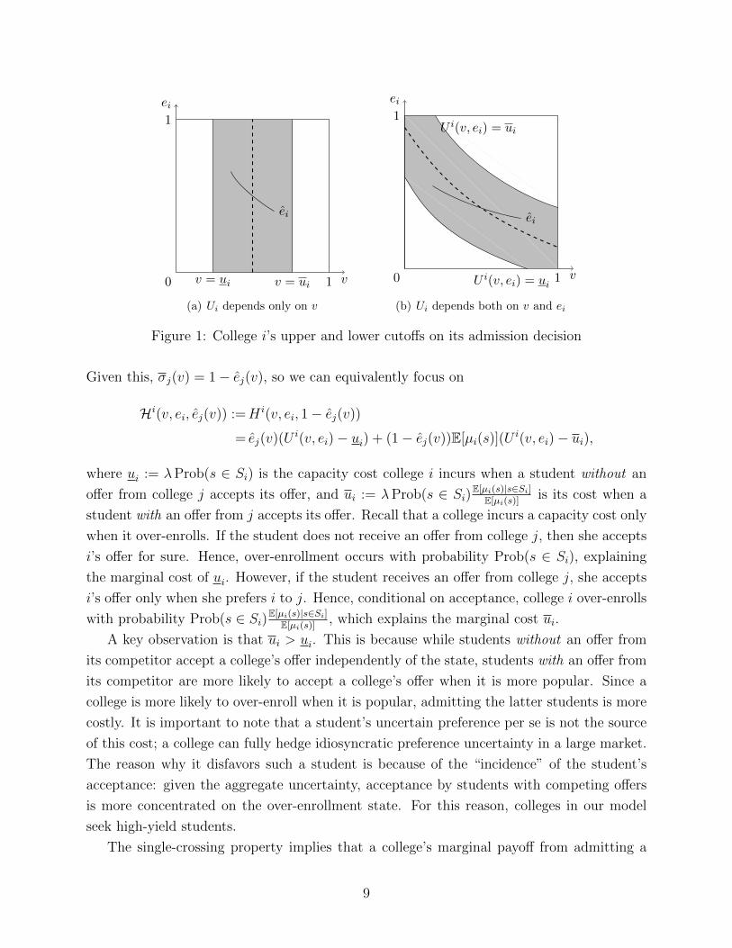
Figure 1: College i’s upper and lower cutoffs on its admission decision

Given this, σj(v) = 1− ej(v), so we can equivalently focus on

Hi(v, ei, ej(v)) :=H i(v, ei, 1− ej(v))

= ej(v)(U i(v, ei)− ui) + (1− ej(v))E[µi(s)](Ui(v, ei)− ui),

where ui := λProb(s ∈ Si) is the capacity cost college i incurs when a student without an

offer from college j accepts its offer, and ui := λProb(s ∈ Si)E[µi(s)|s∈Si]E[µi(s)]

is its cost when a

student with an offer from j accepts its offer. Recall that a college incurs a capacity cost only

when it over-enrolls. If the student does not receive an offer from college j, then she accepts

i’s offer for sure. Hence, over-enrollment occurs with probability Prob(s ∈ Si), explaining

the marginal cost of ui. However, if the student receives an offer from college j, she accepts

i’s offer only when she prefers i to j. Hence, conditional on acceptance, college i over-enrolls

with probability Prob(s ∈ Si)E[µi(s)|s∈Si]E[µi(s)]

, which explains the marginal cost ui.

A key observation is that ui > ui. This is because while students without an offer from

its competitor accept a college’s offer independently of the state, students with an offer from

its competitor are more likely to accept a college’s offer when it is more popular. Since a

college is more likely to over-enroll when it is popular, admitting the latter students is more

costly. It is important to note that a student’s uncertain preference per se is not the source

of this cost; a college can fully hedge idiosyncratic preference uncertainty in a large market.

The reason why it disfavors such a student is because of the “incidence” of the student’s

acceptance: given the aggregate uncertainty, acceptance by students with competing offers

is more concentrated on the over-enrollment state. For this reason, colleges in our model

seek high-yield students.

The single-crossing property implies that a college’s marginal payoff from admitting a

9

student of a given score v increases, so its cutoff falls, when its opponent raises its cutoff.

Consequently, the game facing the colleges is one of strategic substitutability. To gain further

understanding, for college i = A,B and for each v ∈ V , define i’s upper and lower cutoffs:12

ei(v) := inf{e|Hi(v, e; 0) ≥ 0} and ei(v) := inf{e|Hi(v, e; 1) ≥ 0},

which are depicted in Figure 1. The left and right panels respectively describe the case that

the colleges only value students’ scores (i.e., U i(v, ei) ≡ v) and the case that they also value

students’ fit. The students with (v, ei) above the upper cutoff are worth admitting even

when the opponent college employs ej(v) = 0 (i.e., j admits all type-v students); surely, it is

optimal for college i to admit such students. Likewise, the students below the lower cutoff

give negative marginal payoff even when they receive no offers from j; surely, it is optimal

for college i to reject them. Inspection of Hi reveals that these two cutoffs correspond to

indifference curves, U i(v, ei) = ui and U i(v, ei) = ui, respectively. The real cutoff ei(·) must

lie between the two cutoffs, in the “gray zone” in Figure 1. The equilibrium cutoffs are

characterized more precisely in the next theorem.

Theorem 1. An equilibrium is characterized by a profile of cutoff functions {(eA(v), eB(v))}v,each of which lies between the upper and lower cutoffs for the respective college, where

ei(v) = inf{e|Hi(v, e; ej(v)) ≥ 0} for i, j = A,B and i 6= j,

(and is equal to one when the set is empty). For each i = A,B, if ei(v) ∈ (0, 1) and ej(v) is

strictly decreasing in v, then

|e′i(v)| < U iv(v, ei)

U iei

(v, ei)

∣∣∣∣ei=ei(v)

, (2)

where the RHS of (2) is infinite if U iei

= 0.

Proof. See Appendix A.3. �

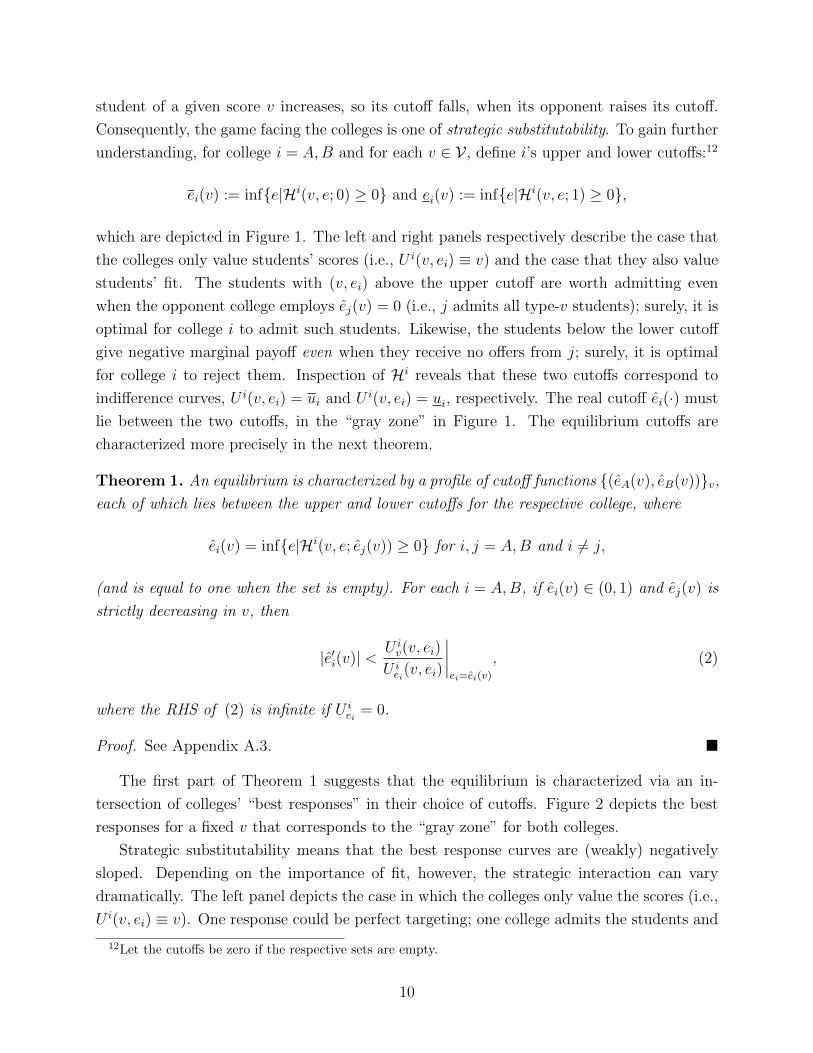
The first part of Theorem 1 suggests that the equilibrium is characterized via an in-

tersection of colleges’ “best responses” in their choice of cutoffs. Figure 2 depicts the best

responses for a fixed v that corresponds to the “gray zone” for both colleges.

Strategic substitutability means that the best response curves are (weakly) negatively

sloped. Depending on the importance of fit, however, the strategic interaction can vary

dramatically. The left panel depicts the case in which the colleges only value the scores (i.e.,

U i(v, ei) ≡ v). One response could be perfect targeting; one college admits the students and

12Let the cutoffs be zero if the respective sets are empty.

10

1

1

0 eA

eB eB

eA

(a) Ui depends only on v

1

1

0 eA

eB eA

eB

(b) Ui depends both on v and ei

Figure 2: Colleges’s best responses for a fixed v corresponding to the “gray zone.”

the other rejects them (either corner). They may also coordinate by “mixing”—or selecting

an interior fraction of students,—by using the ei as a randomization device. Colleges playing

this latter strategy will appear to value the ei even though they are of no intrinsic value to

them. The right panel depicts the case in which colleges value their fit highly. Placing a

large weight on a college-specific attribute lowers enrollment uncertainty and weakens the

strategic link between the colleges. Consequently, the best-response curves are relatively

flat, and a unique (and interior) intersection (e∗i , e∗j) obtains in this case.

Ultimately, one is interested in how the cutoffs (eA(v), eB(v)) vary with v. An interest-

ing question is whether ei(v) is decreasing in v in equilibrium, which would imply that the

equilibrium admissions policy is monotonic: if college i admits a type-(v, ei) student, then

it must also admit a type-(v′, e′i) student, provided (v′, e′i) ≥ (v, ei). Our equilibrium does not

guarantee such a monotonicity; the reason is that, while Hi(v, ei, ej) is increasing in v for a

fixed (ei, ej), Hi(v, ei, e∗j(v)) need not; namely, the strategic response by the opponent can

give rise to a non-monotonic reaction. Indeed, non-monotonicities may arise in equilibrium

when the colleges primarily value the score, as will be seen below. Even when the admission

policies are monotonic, the colleges do not admit students according to their intrinsic pref-

erences. Indeed, the second part of Theorem 1 reveals that colleges systematically distort

the admissions criteria to favor those students who rank highly in fit at the expense of those

who rank highly in scores. The “overweighting” of fit (or a college-specific attribute) is seen

formally by the fact that the slope of the cutoff curve ei(·) is less than that of the indifference

curve, i.e., the college’s true marginal rate of substitution of v for ei.

More precise understanding of the equilibrium can be gained by focusing on two special

cases, to which we now turn.

11

(a) College A

(b) College B

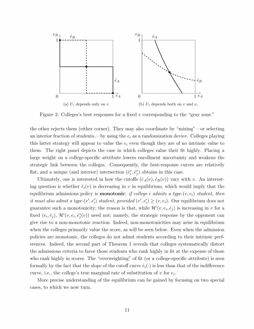
Figure 3: Colleges’ admission strategies when they only value v. We assume v ∼ U [0, 1],λ = 20, κ = 0.36 and µ(s) = 1

2s+ 2

5.

� Colleges only value the score.

As mentioned, in this case, colleges may strategically target or mix over the students in the

gray zone. We focus on the equilibrium in which each college i = A,B mixes over the students

using ei as a randomization device. More precisely, in a mixing equilibrium, they choose

(eA(v), eB(v)) so thatHi(v, ei(v), ej(v)) = 0 for any v ∈ (max{uA, uB},min{uA, uB}).13 Such

an equilibrium always exists, as will be shown below.14

The example depicted in Figure 3 shows equilibrium admissions strategies when college A

is slightly more popular than college B. In line with Figure 1(a), both upper and lower cutoffs

are step functions, indexed by their vertical segments. Interestingly, the vertical segments

13Since the upper and lower cutoffs are endogenous, it is a priori unclear if this gray zone would be non-empty in equilibrium. Theorem 2 provides a sufficient condition for the gray zone to appear in equilibrium.

14There may exist another equilibrium in which colleges target students perfectly based on v, as depictedby a corner intersection in Figure 2(a). Such an equilibrium requires a great deal of coordination betweencolleges that may be implausible, whereas the “mixing” equilibrium is more “anonymous” in the way thecolleges treat different v types. The welfare and fairness implications we report in Theorem 4 also apply tothis perfect coordinating equilibrium, however.

12

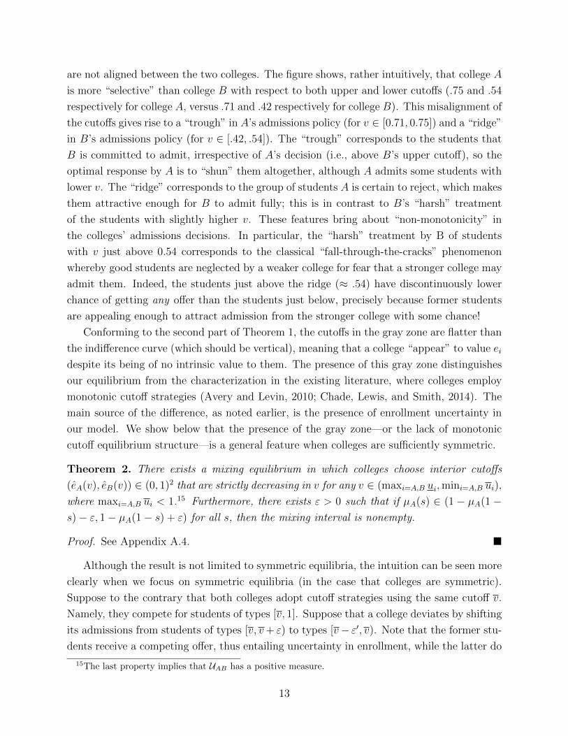
are not aligned between the two colleges. The figure shows, rather intuitively, that college A

is more “selective” than college B with respect to both upper and lower cutoffs (.75 and .54

respectively for college A, versus .71 and .42 respectively for college B). This misalignment of

the cutoffs gives rise to a “trough” in A’s admissions policy (for v ∈ [0.71, 0.75]) and a “ridge”

in B’s admissions policy (for v ∈ [.42, .54]). The “trough” corresponds to the students that

B is committed to admit, irrespective of A’s decision (i.e., above B’s upper cutoff), so the

optimal response by A is to “shun” them altogether, although A admits some students with

lower v. The “ridge” corresponds to the group of students A is certain to reject, which makes

them attractive enough for B to admit fully; this is in contrast to B’s “harsh” treatment

of the students with slightly higher v. These features bring about “non-monotonicity” in

the colleges’ admissions decisions. In particular, the “harsh” treatment by B of students

with v just above 0.54 corresponds to the classical “fall-through-the-cracks” phenomenon

whereby good students are neglected by a weaker college for fear that a stronger college may

admit them. Indeed, the students just above the ridge (≈ .54) have discontinuously lower

chance of getting any offer than the students just below, precisely because former students

are appealing enough to attract admission from the stronger college with some chance!

Conforming to the second part of Theorem 1, the cutoffs in the gray zone are flatter than

the indifference curve (which should be vertical), meaning that a college “appear” to value ei

despite its being of no intrinsic value to them. The presence of this gray zone distinguishes

our equilibrium from the characterization in the existing literature, where colleges employ

monotonic cutoff strategies (Avery and Levin, 2010; Chade, Lewis, and Smith, 2014). The

main source of the difference, as noted earlier, is the presence of enrollment uncertainty in

our model. We show below that the presence of the gray zone—or the lack of monotonic

cutoff equilibrium structure—is a general feature when colleges are sufficiently symmetric.

Theorem 2. There exists a mixing equilibrium in which colleges choose interior cutoffs

(eA(v), eB(v)) ∈ (0, 1)2 that are strictly decreasing in v for any v ∈ (maxi=A,B ui,mini=A,B ui),

where maxi=A,B ui < 1.15 Furthermore, there exists ε > 0 such that if µA(s) ∈ (1 − µA(1 −s)− ε, 1− µA(1− s) + ε) for all s, then the mixing interval is nonempty.

Proof. See Appendix A.4. �

Although the result is not limited to symmetric equilibria, the intuition can be seen more

clearly when we focus on symmetric equilibria (in the case that colleges are symmetric).

Suppose to the contrary that both colleges adopt cutoff strategies using the same cutoff v.

Namely, they compete for students of types [v, 1]. Suppose that a college deviates by shifting

its admissions from students of types [v, v+ ε) to types [v− ε′, v). Note that the former stu-

dents receive a competing offer, thus entailing uncertainty in enrollment, while the latter do

15The last property implies that UAB has a positive measure.

13

not. For small enough ε and ε′, chosen to keep the expected yield unchanged, the resulting

drop in the quality of the admission pool is negligible but the benefit in reducing the un-

certainty is of first-order importance. Hence, the (symmetric) monotonic cutoff equilibrium

cannot be sustained.16

� Colleges value fit significantly.

In this case, colleges’ preferences are sufficiently independent, so their incentive to strate-

gically target students based on v is not very strong. Hence, the equilibrium admissions

strategies are now likely to exhibit monotonicity. However, as stated in Theorem 1, the yield

management consideration will still cause them to bias their admissions policies in favor of

students with high fit.

To state the result formally, we assume that there exists δ > 0 such that U iv(v,ei)U i(v,ei)

≤ δUjv (v,ej)

Uj(v,ej)

for all (v, ei, ej) ∈ (0, 1)3, where i, j = A,B and i 6= j.17 We further assume that

U i(v, 0) = 0 andU iei

(v, ei)

U i(v, ei)> max

{1− µiµi

,µi

1− µiδ

}for all (v, ei), (3)

where µi := E[µi(s)] for i = A,B. This condition implies that colleges value fit sufficiently

highly, relative to the score.

Theorem 3. Given (3), an equilibrium exists, and in any equilibrium, college i’s cutoff

ei(v) is nonincreasing in v everywhere and strictly decreasing in v whenever ei(v) ∈ (0, 1).

In particular, there exists v < 1 such that for all v > v, (eA(v), eB(v)) are strictly decreasing

in v (hence UAB has a positive measure). The colleges overweight fit in the sense of (2) for

v > v.

Proof. See Appendix A.5. �

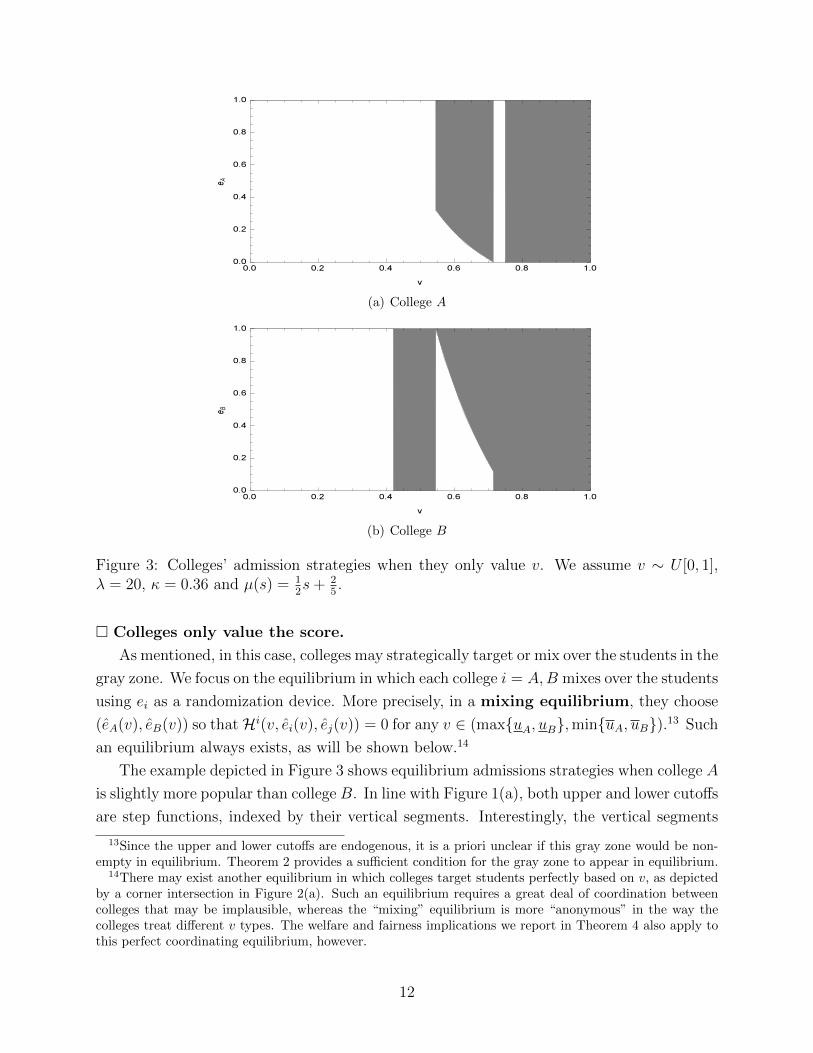
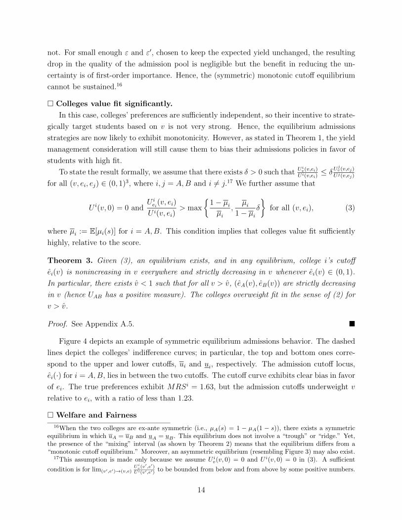
Figure 4 depicts an example of symmetric equilibrium admissions behavior. The dashed

lines depict the colleges’ indifference curves; in particular, the top and bottom ones corre-

spond to the upper and lower cutoffs, ui and ui, respectively. The admission cutoff locus,

ei(·) for i = A,B, lies in between the two cutoffs. The cutoff curve exhibits clear bias in favor

of ei. The true preferences exhibit MRSi = 1.63, but the admission cutoffs underweight v

relative to ei, with a ratio of less than 1.23.

� Welfare and Fairness

16When the two colleges are ex-ante symmetric (i.e., µA(s) = 1 − µA(1 − s)), there exists a symmetricequilibrium in which uA = uB and uA = uB . This equilibrium does not involve a “trough” or “ridge.” Yet,the presence of the “mixing” interval (as shown by Theorem 2) means that the equilibrium differs from a“monotonic cutoff equilibrium.” Moreover, an asymmetric equilibrium (resembling Figure 3) may also exist.

17This assumption is made only because we assume U iv(v, 0) = 0 and U i(v, 0) = 0 in (3). A sufficient

condition is for lim(v′,e′)→(v,e)Ui

v(v′,e′)

Ui(v′,e′) to be bounded from below and from above by some positive numbers.

14

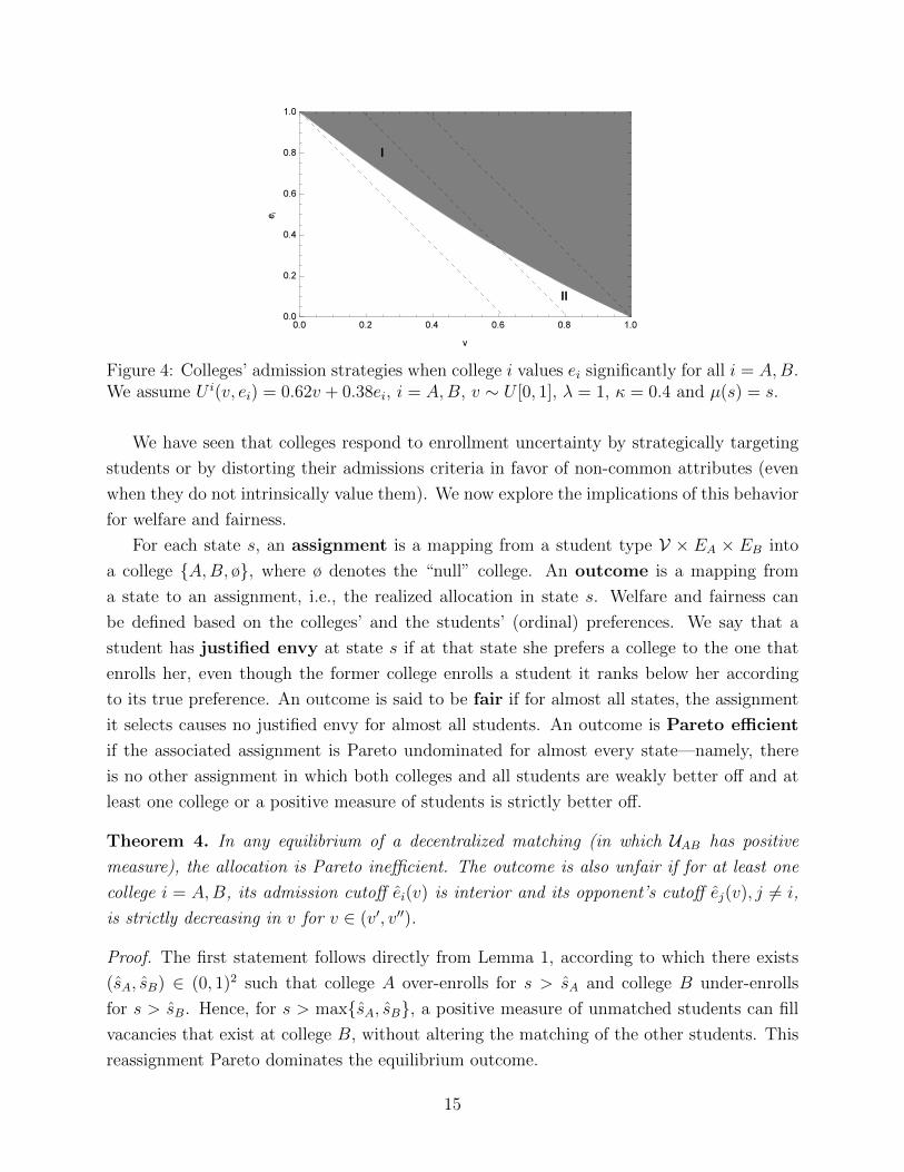
Figure 4: Colleges’ admission strategies when college i values ei significantly for all i = A,B.We assume U i(v, ei) = 0.62v + 0.38ei, i = A,B, v ∼ U [0, 1], λ = 1, κ = 0.4 and µ(s) = s.

We have seen that colleges respond to enrollment uncertainty by strategically targeting

students or by distorting their admissions criteria in favor of non-common attributes (even

when they do not intrinsically value them). We now explore the implications of this behavior

for welfare and fairness.

For each state s, an assignment is a mapping from a student type V × EA × EB into

a college {A,B, ø}, where ø denotes the “null” college. An outcome is a mapping from

a state to an assignment, i.e., the realized allocation in state s. Welfare and fairness can

be defined based on the colleges’ and the students’ (ordinal) preferences. We say that a

student has justified envy at state s if at that state she prefers a college to the one that

enrolls her, even though the former college enrolls a student it ranks below her according

to its true preference. An outcome is said to be fair if for almost all states, the assignment

it selects causes no justified envy for almost all students. An outcome is Pareto efficient

if the associated assignment is Pareto undominated for almost every state—namely, there

is no other assignment in which both colleges and all students are weakly better off and at

least one college or a positive measure of students is strictly better off.

Theorem 4. In any equilibrium of a decentralized matching (in which UAB has positive

measure), the allocation is Pareto inefficient. The outcome is also unfair if for at least one

college i = A,B, its admission cutoff ei(v) is interior and its opponent’s cutoff ej(v), j 6= i,

is strictly decreasing in v for v ∈ (v′, v′′).

Proof. The first statement follows directly from Lemma 1, according to which there exists

(sA, sB) ∈ (0, 1)2 such that college A over-enrolls for s > sA and college B under-enrolls

for s > sB. Hence, for s > max{sA, sB}, a positive measure of unmatched students can fill

vacancies that exist at college B, without altering the matching of the other students. This

reassignment Pareto dominates the equilibrium outcome.

15

To prove the latter claim, suppose ei(v) ∈ (0, 1) and ej(v) is strictly decreasing in v for

an interval (v′, v′′). By the second part of Theorem 1, we have |e′i(v)| < U iv(v,ei)

U iei

(v,ei)

∣∣ei=ei(v)

. This

means that one can find two sets of students X, X ⊂ (v′, v′′) × Ei and u such that, for all

(v, e) ∈ X, e > ei(v) and U i(e, v) < u, and for all (v, e) ∈ X, e < ei(v) and U i(v, e) > u. (In

Figure 4, X can be found in region I, at the top between solid and dotted lines, and X can

be found in region II, at the bottom between dotted and solid lines). Clearly, the students

in X have justified envy toward students in X. Since the justified envy exists for a positive

measure of students for all states, the outcome is unfair. �

Theorem 2 and Theorem 3 give sufficient conditions for the outcome to be unfair.

Corollary 1. The outcome is unfair in any equilibrium given (3) or in the mixing equilibrium

of the one dimensional model if the colleges are sufficiently symmetric.

4 Different Responses to Enrollment Uncertainty

In this section, we study additional measures that colleges may employ to manage their

enrollment. We focus on the environment in which colleges only value the score v throughout

this section.

4.1 Restricted Applications

One common method colleges employ is to limit the number of applications that students

can submit. The restriction may be coordinated by colleges, or even institutionalized, as in

the UK, Korea and Japan.18 It may also be a result of colleges’ unilateral actions, as with

the “single-choice” requirement some US colleges place in their early admissions plans,19 or

with the synchronized scheduling of on-site entrance exams by colleges in Korea and Japan.20

Restricting applications eases colleges’ burden of managing uncertainty in enrollment;

yield rates rise because applicants have fewer choices and students are forced to become

18Students cannot apply to both Cambridge and Oxford in the UK, and applicants in Japan can apply toat most two public universities. Korean colleges (more precisely, college-department pairs) are partitionedinto three groups, and students are allowed to apply to only one in each group.

19Early admissions consist of Early Decision, which requires students to enroll if admitted, and EarlyAction, which does not involve such commitment. While pursuing admission under an Early Decision plan,students may apply to other institutions, but may have only one Early Decision application pending at anytime (NACAC, 2012). Some Early Action plans place restrictions on student applications to other earlyplans. Selective universities such as Harvard, Stanford, Yale and Princeton restricted applicants to a singleprivate university in their 2014 Early Action plans.

20The Korean government has offered several dates, and many Korean universities have voluntarily chosento schedule their exam on the same date. See Avery, Lee, and Roth (2014) about the colleges’ strategicscheduling problem in such an environment. Public universities in Japan coordinate on three dates foron-site entrance exams.

16

y

vA(a)

vB(a)0

1v

1 y12

(a) State a

y

vA(b)

vB(b)

0

1v

1 y12

(b) State b

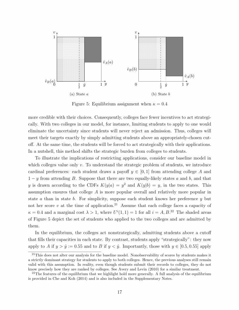
Figure 5: Equilibrium assignment when κ = 0.4

more credible with their choices. Consequently, colleges face fewer incentives to act strategi-

cally. With two colleges in our model, for instance, limiting students to apply to one would

eliminate the uncertainty since students will never reject an admission. Thus, colleges will

meet their targets exactly by simply admitting students above an appropriately-chosen cut-

off. At the same time, the students will be forced to act strategically with their applications.

In a nutshell, this method shifts the strategic burden from colleges to students.

To illustrate the implications of restricting applications, consider our baseline model in

which colleges value only v. To understand the strategic problem of students, we introduce

cardinal preferences: each student draws a payoff y ∈ [0, 1] from attending college A and

1− y from attending B. Suppose that there are two equally-likely states a and b, and that

y is drawn according to the CDFs K(y|a) = y2 and K(y|b) = y, in the two states. This

assumption ensures that college A is more popular overall and relatively more popular in

state a than in state b. For simplicity, suppose each student knows her preference y but

not her score v at the time of application.21 Assume that each college faces a capacity of

κ = 0.4 and a marginal cost λ > 1, where U i(1, 1) = 1 for all i = A,B.22 The shaded areas

of Figure 5 depict the set of students who applied to the two colleges and are admitted by

them.

In the equilibrium, the colleges act nonstrategically, admitting students above a cutoff

that fills their capacities in each state. By contrast, students apply “strategically”: they now

apply to A if y > y := 0.55 and to B if y < y. Importantly, those with y ∈ [0.5, 0.55] apply

21This does not alter our analysis for the baseline model. Nonobservability of scores by students makes ita strictly dominant strategy for students to apply to both colleges. Hence, the previous analyses still remainvalid with this assumption. In reality, even though students submit their records to colleges, they do notknow precisely how they are ranked by colleges. See Avery and Levin (2010) for a similar treatment.

22The features of the equilibrium that we highlight hold more generally. A full analysis of the equilibriumis provided in Che and Koh (2014) and is also included in the Supplementary Notes.

17

to B despite the fact that they prefer A to B. This is because of the overall popularity of

A, which causes these students to sacrifice their moderate preference for A so as to increase

the odds of getting admitted by any college.

One can see that the shifting of strategic burden from colleges to students does not

eliminate the fairness and welfare problems of congestion. First, the equilibrium is unfair.

Justified envy arises in state a for students with (v, y) ∈ [0, vA(a)]×[0.5, 1] who are unassigned

despite having scores exceeding B’s cutoff of vB(a) = 0, and it arises in state b for students

with (v, y) ∈ [vA(b), 1]× [0.5, 0.55] who get into B even though they prefer A and have scores

above its cutoff vA(b). Second, the equilibrium is inefficient. In state a, only mass 0.3 of

students apply to B, leaving its capacity κ = 0.4 unfilled. This outcome is inefficient because

some students are unmatched even though they are acceptable to B in that state.

4.2 Sequential Admissions: Wait-listing

Colleges also manage enrollment uncertainty by offering admissions sequentially. According

to this method, a college admits some applicants and wait-list others in the first round.

Later it admits students from the wait list when some offers are rejected. This process may

repeat for several rounds. Most colleges in France and Korea use wait lists. In the US,

nearly 45% of four-year colleges adopted wait lists in 2011, up from 32% in 2002 (NACAC,

2012). Typically, admissions in each round are not deferred and/or the number of iterations

is limited. Hence, even though wait-listing allows for more admission offers and acceptances

than the baseline model, it does not fully eliminate congestion. For this reason, strategic

targeting remains an issue.23

This point can be seen by a simple extension of our baseline model. There are three

colleges, A, B and C, each with a mass κ < 13

capacity. Colleges again evaluate students

based only on their common score v, as before. All students prefer A and B to C, but C is

significantly better than not attending any school. A college’s utility is given by students’

scores, but for each student, there is a probability ε ∈ (0, 1) that each of colleges A and B

finds the student unacceptable. College C admits students simply based on their scores.

There are two equally-likely states, a and b. In state j ∈ {a, b}, a fraction sj of students

gets utility u from A and u′ < u from B, and the remaining 1−sj students have the opposite

preference, where sa = 1 − sb > 12. (In other words, college i is more popular in state si,

23While allowing for many iterations will ease the problem, the design of the market still matters. Inprinciple, the market for clinical psychologists admits numerous rounds of iterations, but suffers from con-gestion (Roth and Xing (1997)). Korean college admissions involve many rounds, but nontrivial congestionappears to exist, as we show below (see Section 5). Another measure of congestion is the number of “repeatapplicants”—the applicants who are either unmatched or refuse to accept their assignments and wait onefull year to take another “crack” at the assignment process. That number reached 127,000 in Korea in 2014.While much of the problem may be solved by a “frictionless aftermarket,” what form the market should takeis far from clear.

18

i = A,B, and the two colleges are ex ante symmetric in popularity.) In either state, a

student gets utility u′′ from C, where (1−ε)u < u′′ < u, so having C with certainty is better

than having the more preferred of the two other colleges with probability 1− ε. In addition,

suppose that λ is so high that a college never admits more than κ in total. Consider the

following model of wait-listing: in each round, each college admits a set of students and wait-

lists the remaining applicants. A student who has received an offer must accept or reject it

immediately. After the first round, colleges A and B learn the state, so the game effectively

ends in two rounds.

We show that there is no symmetric equilibrium in which both colleges A and B use a

cutoff strategy (i.e., admit the top κ acceptable students) in the first round.

Theorem 5. There is no symmetric equilibrium in which both colleges A and B offer ad-

missions to the top κ acceptable students in the first round.

Proof. See Appendix A.6. �

The intuition behind this result is as follows. Suppose A and B admit the best candidates

up to their capacities while keeping the next best group in mind in case some offers are turned

down. The problem with this strategy is that when some of those admitted turn down their

offers, the next-best students the colleges have in mind may not be available, since these

students, uncertain about whether A or B would find them acceptable, may have accepted

an offer from C. This implies that the students who remain after the first round are likely to

be far worse than the next-best group. Hence, a college would deviate profitably by skipping

over some of the top κ students and preemptively admitting some of the second-best students.

Theorem 5 implies that strategic targeting—i.e., a non-monotonic equilibrium—must occur

in any symmetric equilibrium, and this also implies that the outcome will be, in general,

unfair and inefficient.

4.3 Centralized Matching via Deferred Acceptance

The most systemic response to enrollment uncertainty is to centralize the admissions via

a clearinghouse. College admissions are centralized in countries such as Australia, China,

Germany, Taiwan, Turkey and the UK. While a number of matching algorithms may be used

for this purpose, one popular method is Gale and Shapley’s Deferred Acceptance algorithm

(henceforth DA). Not only is DA employed in many centralized markets, such as public

school admissions and medical residency assignments, but it also has a number of desirable

properties compared to decentralized matching, as we shall highlight below.

In the DA algorithm (student-proposing version), students and colleges report their or-

dinal preferences to the clearinghouse, which then uses the information to simulate the

19

vA(s)

vB(s)

0

1v

1 y12

(a) Round 1

vA(s)

vB(s)

0

1v

1 y12

(b) Round 2

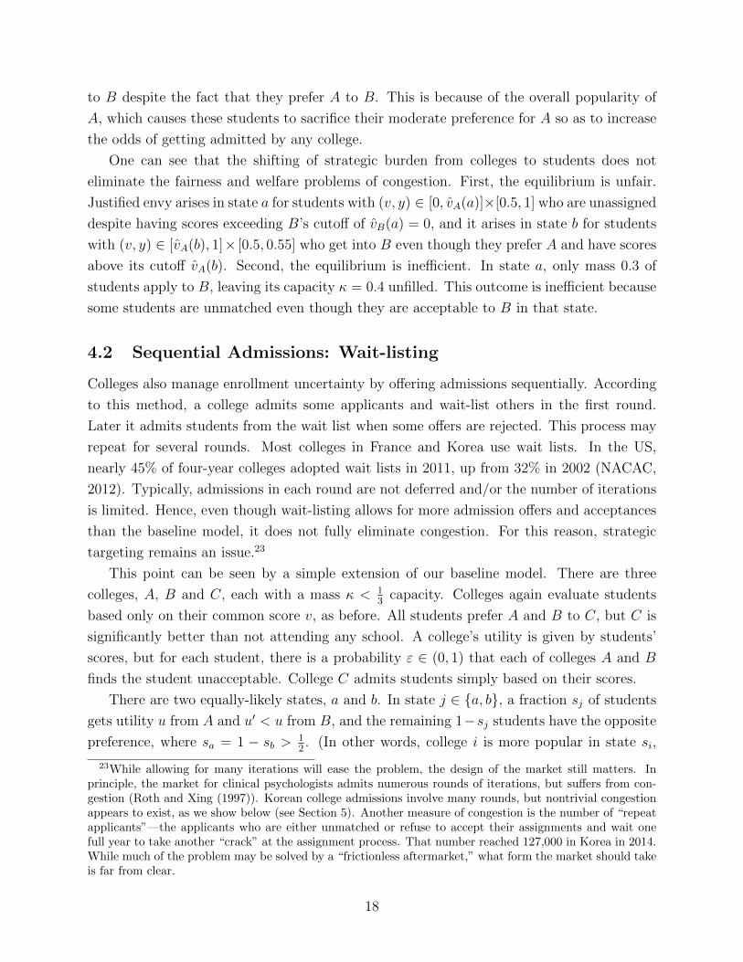
Figure 6: Deferred Acceptance Algorithm

following multi-round procedure. In each round t = 1, ..., students apply to the most pre-

ferred colleges that have not yet rejected them. The colleges then tentatively accept the most

preferred applicants up to their capacities and reject the rest (permanently). This process

is repeated until no further applications are made, in which case each student is assigned

to a college that has tentatively accepted the student. While the sequential nature of the

mechanism resembles the “wait-listing” considered earlier, it differs in several respects: first,

students apply to one college per round; second, a college’s admission is tentative in each

round; and third, the number of rounds is not limited. These features eliminate congestion.

To see this, consider how DA would proceed in our baseline model with only score v

(assuming truthful reporting by agents on both sides). For concreteness, fix a realized

state s such that µA(s) > 1/2. DA takes two rounds, and Figure 6 describes the set of

students who apply to the two colleges and are admitted by them in each of the two rounds.

In the first round, a mass µA(s) of students apply to college A, and the remaining mass

µB(s) = 1 − µA(s) of students apply to college B. Each college tentatively admits the top

κ students among the applicants. Thus, colleges’ cutoffs in this round, denoted by vi(s),

satisfy µi(s)(1 − G(vi(s))) = κ for i = A,B (see Figure 6(a)). The rejected students then

apply to the remaining college in the second round, and again, colleges reselect the top κ

students among those admitted tentatively in the first round and the new applicants. Thus,

colleges’ cutoffs are readjusted to satisfy µA(s)(1 − G(vA(s))) = κ and 1 − G(vB(s)) = 2κ

(see Figure 6(b)). Since there are no more colleges to which rejected students can apply, the

algorithm terminates, and the tentative assignment becomes final. The outcome is clearly

fair since a student never envies another with a lower score v, and it is also Pareto efficient.

More generally, the following results hold for our baseline model.

Theorem 6. DA makes truthful reporting a weakly dominant strategy for students and it

20

makes truthful reporting of rankings (based on v) and capacities an ex post equilibrium for

colleges. In the resulting equilibrium, in each state s, there are cutoffs (vA(s), vB(s)) such

that each student v is assigned to the best college among those whose cutoff is below v, and

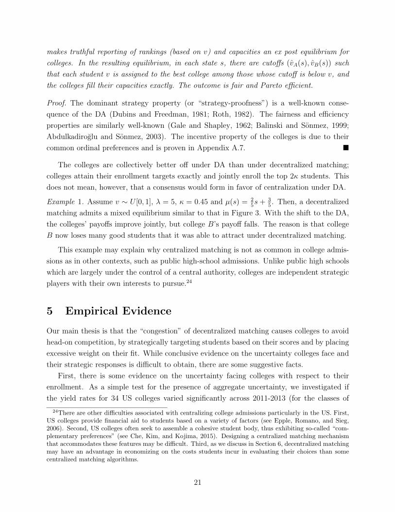
the colleges fill their capacities exactly. The outcome is fair and Pareto efficient.

Proof. The dominant strategy property (or “strategy-proofness”) is a well-known conse-

quence of the DA (Dubins and Freedman, 1981; Roth, 1982). The fairness and efficiency

properties are similarly well-known (Gale and Shapley, 1962; Balinski and Sonmez, 1999;

Abdulkadiroglu and Sonmez, 2003). The incentive property of the colleges is due to their

common ordinal preferences and is proven in Appendix A.7. �

The colleges are collectively better off under DA than under decentralized matching;

colleges attain their enrollment targets exactly and jointly enroll the top 2κ students. This

does not mean, however, that a consensus would form in favor of centralization under DA.

Example 1. Assume v ∼ U [0, 1], λ = 5, κ = 0.45 and µ(s) = 25s + 3

5. Then, a decentralized

matching admits a mixed equilibrium similar to that in Figure 3. With the shift to the DA,

the colleges’ payoffs improve jointly, but college B’s payoff falls. The reason is that college

B now loses many good students that it was able to attract under decentralized matching.

This example may explain why centralized matching is not as common in college admis-

sions as in other contexts, such as public high-school admissions. Unlike public high schools

which are largely under the control of a central authority, colleges are independent strategic

players with their own interests to pursue.24

5 Empirical Evidence

Our main thesis is that the “congestion” of decentralized matching causes colleges to avoid

head-on competition, by strategically targeting students based on their scores and by placing

excessive weight on their fit. While conclusive evidence on the uncertainty colleges face and

their strategic responses is difficult to obtain, there are some suggestive facts.

First, there is some evidence on the uncertainty facing colleges with respect to their

enrollment. As a simple test for the presence of aggregate uncertainty, we investigated if

the yield rates for 34 US colleges varied significantly across 2011-2013 (for the classes of

24There are other difficulties associated with centralizing college admissions particularly in the US. First,US colleges provide financial aid to students based on a variety of factors (see Epple, Romano, and Sieg,2006). Second, US colleges often seek to assemble a cohesive student body, thus exhibiting so-called “com-plementary preferences” (see Che, Kim, and Kojima, 2015). Designing a centralized matching mechanismthat accommodates these features may be difficult. Third, as we discuss in Section 6, decentralized matchingmay have an advantage in economizing on the costs students incur in evaluating their choices than somecentralized matching algorithms.

21

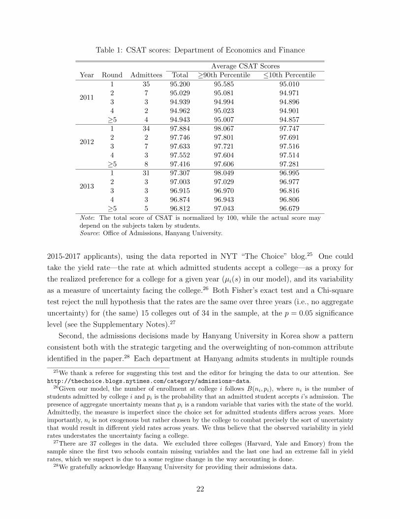
Table 1: CSAT scores: Department of Economics and Finance

Average CSAT ScoresYear Round Admittees Total ≥90th Percentile ≤10th Percentile

2011

1 35 95.200 95.585 95.0102 7 95.029 95.081 94.9713 3 94.939 94.994 94.8964 2 94.962 95.023 94.901≥5 4 94.943 95.007 94.857

2012

1 34 97.884 98.067 97.7472 2 97.746 97.801 97.6913 7 97.633 97.721 97.5164 3 97.552 97.604 97.514≥5 8 97.416 97.606 97.281

2013

1 31 97.307 98.049 96.9952 3 97.003 97.029 96.9773 3 96.915 96.970 96.8164 3 96.874 96.943 96.806≥5 5 96.812 97.043 96.679

Note: The total score of CSAT is normalized by 100, while the actual score maydepend on the subjects taken by students.Source: Office of Admissions, Hanyang University.

2015-2017 applicants), using the data reported in NYT “The Choice” blog.25 One could

take the yield rate—the rate at which admitted students accept a college—as a proxy for

the realized preference for a college for a given year (µi(s) in our model), and its variability

as a measure of uncertainty facing the college.26 Both Fisher’s exact test and a Chi-square

test reject the null hypothesis that the rates are the same over three years (i.e., no aggregate

uncertainty) for (the same) 15 colleges out of 34 in the sample, at the p = 0.05 significance

level (see the Supplementary Notes).27

Second, the admissions decisions made by Hanyang University in Korea show a pattern

consistent both with the strategic targeting and the overweighting of non-common attribute

identified in the paper.28 Each department at Hanyang admits students in multiple rounds

25We thank a referee for suggesting this test and the editor for bringing the data to our attention. Seehttp://thechoice.blogs.nytimes.com/category/admissions-data.

26Given our model, the number of enrollment at college i follows B(ni, pi), where ni is the number ofstudents admitted by college i and pi is the probability that an admitted student accepts i’s admission. Thepresence of aggregate uncertainty means that pi is a random variable that varies with the state of the world.Admittedly, the measure is imperfect since the choice set for admitted students differs across years. Moreimportantly, ni is not exogenous but rather chosen by the college to combat precisely the sort of uncertaintythat would result in different yield rates across years. We thus believe that the observed variability in yieldrates understates the uncertainty facing a college.

27There are 37 colleges in the data. We excluded three colleges (Harvard, Yale and Emory) from thesample since the first two schools contain missing variables and the last one had an extreme fall in yieldrates, which we suspect is due to a some regime change in the way accounting is done.

28We gratefully acknowledge Hanyang University for providing their admissions data.

22

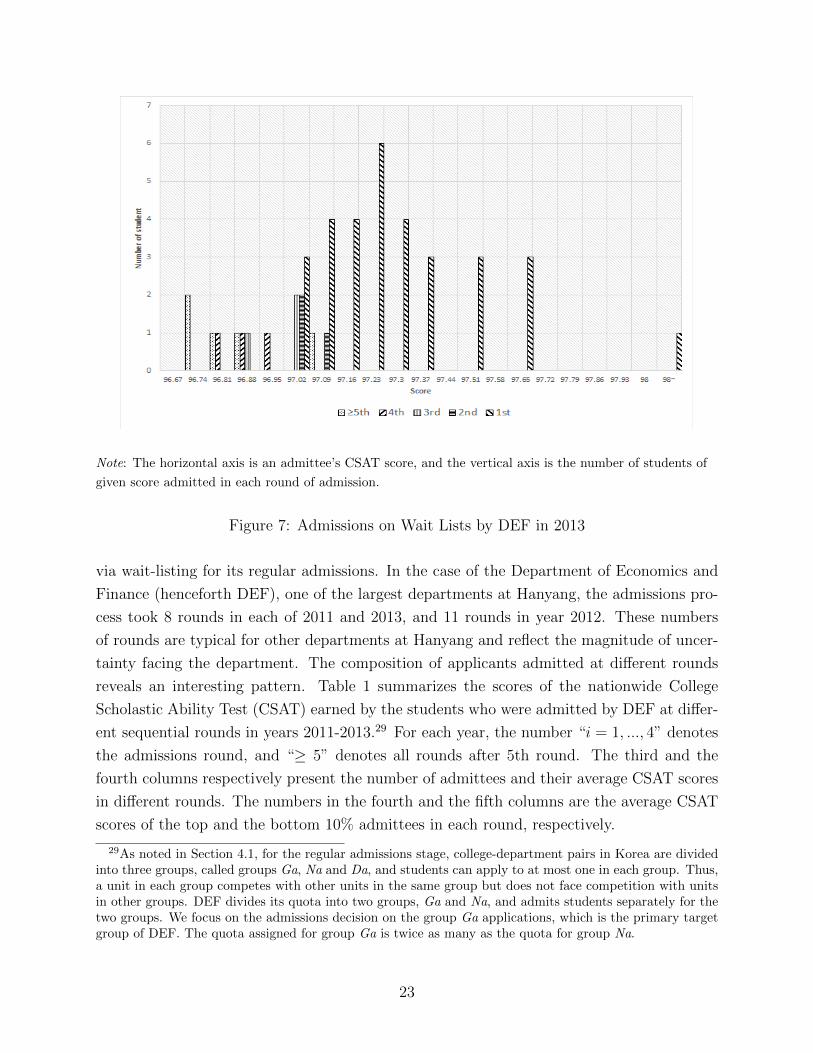
Note: The horizontal axis is an admittee’s CSAT score, and the vertical axis is the number of students of

given score admitted in each round of admission.

Figure 7: Admissions on Wait Lists by DEF in 2013

via wait-listing for its regular admissions. In the case of the Department of Economics and

Finance (henceforth DEF), one of the largest departments at Hanyang, the admissions pro-

cess took 8 rounds in each of 2011 and 2013, and 11 rounds in year 2012. These numbers

of rounds are typical for other departments at Hanyang and reflect the magnitude of uncer-

tainty facing the department. The composition of applicants admitted at different rounds

reveals an interesting pattern. Table 1 summarizes the scores of the nationwide College

Scholastic Ability Test (CSAT) earned by the students who were admitted by DEF at differ-

ent sequential rounds in years 2011-2013.29 For each year, the number “i = 1, ..., 4” denotes

the admissions round, and “≥ 5” denotes all rounds after 5th round. The third and the

fourth columns respectively present the number of admittees and their average CSAT scores

in different rounds. The numbers in the fourth and the fifth columns are the average CSAT

scores of the top and the bottom 10% admittees in each round, respectively.

29As noted in Section 4.1, for the regular admissions stage, college-department pairs in Korea are dividedinto three groups, called groups Ga, Na and Da, and students can apply to at most one in each group. Thus,a unit in each group competes with other units in the same group but does not face competition with unitsin other groups. DEF divides its quota into two groups, Ga and Na, and admits students separately for thetwo groups. We focus on the admissions decision on the group Ga applications, which is the primary targetgroup of DEF. The quota assigned for group Ga is twice as many as the quota for group Na.

23

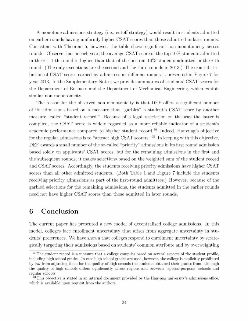
A monotone admissions strategy (i.e., cutoff strategy) would result in students admitted

on earlier rounds having uniformly higher CSAT scores than those admitted in later rounds.

Consistent with Theorem 5, however, the table shows significant non-monotonicity across

rounds. Observe that in each year, the average CSAT score of the top 10% students admitted

in the i + 1-th round is higher than that of the bottom 10% students admitted in the i-th

round. (The only exceptions are the second and the third rounds in 2013.) The exact distri-

bution of CSAT scores earned by admittees at different rounds is presented in Figure 7 for

year 2013. In the Supplementary Notes, we provide summaries of students’ CSAT scores for

the Department of Business and the Department of Mechanical Engineering, which exhibit

similar non-monotonicity.

The reason for the observed non-monotonicity is that DEF offers a significant number

of its admissions based on a measure that “garbles” a student’s CSAT score by another

measure, called “student record.” Because of a legal restriction on the way the latter is

complied, the CSAT score is widely regarded as a more reliable indicator of a student’s

academic performance compared to his/her student record.30 Indeed, Hanynag’s objective

for the regular admissions is to “attract high CSAT scorers.”31 In keeping with this objective,

DEF awards a small number of the so-called “priority” admissions in its first round admission

based solely on applicants’ CSAT scores, but for the remaining admissions in the first and

the subsequent rounds, it makes selections based on the weighted sum of the student record

and CSAT scores. Accordingly, the students receiving priority admissions have higher CSAT

scores than all other admitted students. (Both Table 1 and Figure 7 include the students

receiving priority admissions as part of the first-round admittees.) However, because of the

garbled selections for the remaining admissions, the students admitted in the earlier rounds

need not have higher CSAT scores than those admitted in later rounds.

6 Conclusion

The current paper has presented a new model of decentralized college admissions. In this

model, colleges face enrollment uncertainty that arises from aggregate uncertainty in stu-

dents’ preferences. We have shown that colleges respond to enrollment uncertainty by strate-

gically targeting their admissions based on students’ common attribute and by overweighting

30The student record is a measure that a college compiles based on several aspects of the student profile,including high school grades. In case high school grades are used, however, the college is explicitly prohibitedby law from adjusting them for the quality of high schools the students obtained their grades from, althoughthe quality of high schools differs significantly across regions and between “special-purpose” schools andregular schools.

31This objective is stated in an internal document provided by the Hanyang university’s admissions office,which is available upon request from the authors.

24

their non-common attributes in admissions, and that this equilibrium behavior leads to jus-

tified envy and Pareto inefficiency.

We have also studied other responses by colleges whereby they limit the number of a

student’s applications, admit students in multiple rounds via wait-listing, or centralize ad-

missions via DA. Both restricted application and wait-listing alleviate colleges’ yield control

burden, but strategic targeting and enrollment uncertainty remain, leaving justified envy and

inefficiency unaddressed. Centralized matching via DA achieves efficiency and eliminates

enrollment uncertainty and justified envy, at least when colleges evaluate students only by

a common measure. However, not all colleges necessarily benefit from such a centralized

matching. This last observation may explain why college admissions remain decentralized

in many countries. Our analyses have several other implications.

Early admissions. Early admissions are widely adopted by colleges in the US and Ko-

rea. Early admissions programs allow students to apply to sponsoring colleges early, and

the colleges in turn process their applications prior to the regular admissions round (with

binding or non-binding requirements for students to accept them early). The remaining

students and seats are then allocated through regular admissions. This process resembles

sequential admissions studied in Section 4.2. In addition, some early admissions programs

restrict applications just as in Section 4.1. Although the model involving both sequential ad-

missions and restricted application is not tractable (especially with aggregate uncertainty),

our analyses imply that these features can help colleges to cope with enrollment uncertainty.

We believe this is an important function of early admissions not emphasized by other recent

papers (Avery and Levin, 2010; Lee, 2009). Despite this benefit to colleges, our analyses

suggest that the outcomes of these programs are unlikely to be efficient or fair.

Loyalty and legacy. It is well documented that colleges favor students who show eagerness

to attend them. Students who signal their interests through campus visits, essays, letters of

intention, or webcam interviews are known to be favored by colleges. According to the 2004

and 2005 NACAC Admission Trends Survey, 59% of the colleges surveyed assigned some level

of importance to a student’s “demonstrated interest” in their admissions decisions. Table 2

shows the extent to which certain applicant activities would be considered as a “plus factor”

in the admission process by institutions with varying yield rates.

Early admissions, as Avery and Levin (2010) argue, also serve as a tool for colleges to

identify enthusiastic applicants and favor them in the admission. It is entirely plausible

that these preferences by colleges are intrinsic, as postulated by Avery and Levin (2010).

However, our theory suggests that such a preference could also arise endogenously from the

desire to manage enrollment uncertainty. Like the students without a competing offer in our

25

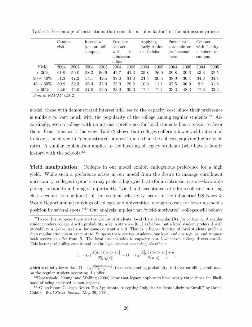
Table 2: Percentage of institutions that consider a “plus factor” in the admission process

Campusvisit

Interview(on or offcampus)

Frequentcontactwith theadmissionoffice

ApplyingEarly Actionor Decision

Particularacademic orprofessionalfocus

Contactwith facultymembers oncampus

Yield 2004 2005 2004 2005 2004 2005 2004 2005 2004 2005 2004 2005

< 30% 61.9 59.0 58.3 56.6 42.7 41.3 35.8 26.9 39.8 39.6 43.3 38.530 ∼ 40% 51.3 47.2 54.1 42.5 37.0 34.0 24.4 26.5 38.0 36.4 34.8 34.446 ∼ 60% 30.9 32.3 36.3 32.3 25.9 26.2 10.3 11.1 32.5 36.9 8.9 31.8> 60% 32.6 45.0 37.0 52.5 23.9 39.3 17.4 7.3 33.3 48.3 17.8 32.2

Source: NACAC (2012)

model, those with demonstrated interest add less to the capacity cost, since their preference

is unlikely to vary much with the popularity of the college among regular students.32 Ac-

cordingly, even a college with no intrinsic preference for loyal students has a reason to favor

them. Consistent with this view, Table 2 shows that colleges suffering lower yield rates tend

to favor students with “demonstrated interest” more than the colleges enjoying higher yield

rates. A similar explanation applies to the favoring of legacy students (who have a family

history with the school).33

Yield manipulation. Colleges in our model exhibit endogenous preference for a high

yield. While such a preference arises in our model from the desire to manage enrollment

uncertainty, colleges in practice may prefer a high yield rate for an intrinsic reason—favorable

perception and brand image. Importantly, “yield and acceptance rates for a college’s entering

class account for one-fourth of the ‘student selectivity’ score in the influential US News &

World Report annual rankings of colleges and universities, enough to raise or lower a school’s

position by several spots.”34 Our analysis implies that “yield-motivated” colleges will behave

32To see this, suppose there are two groups of students, loyal (L) and regular (R), for college A. A regularstudent prefers college A with probability µ(s) in state s ∈ [0, 1] as before, but a loyal student prefers A withprobability µL(s) = µ(s) + a, for some constant a > 0. That is, a higher fraction of loyal students prefer Athan regular students at every state. Suppose there are two students, one loyal and one regular, and supposeboth receive an offer from B. The loyal student adds to capacity cost λ whenever college A over-enrolls.This latter probability conditional on the loyal student accepting A’s offer is

(1− sA)E[µL(s)|s > sA]

E[µL(s)]= (1− sA)

E[µ(s)|s > sA] + a

E[µ(s)] + a,

which is strictly lower than (1−sA)E[µ(s)|s>sA]E[µ(s)] , the corresponding probability of A over-enrolling conditional

on the regular student accepting A’s offer.33Espenshade, Chung, and Walling (2004) show that legacy applicants have nearly three times the likeli-

hood of being accepted as non-legacies.34“Glass Floor: Colleges Reject Top Applicants, Accepting Only the Students Likely to Enroll,” by Daniel

Golden, Wall Street Journal, May 29, 2001.

26

similarly to colleges in our model; namely, they will strategically target students overlooked

by stronger colleges and reject students who are unlikely to accept their offers (or are “too

good for them”). This behavior is consistent with anecdotal evidence.35

Information acquisition and evaluation costs. Often students do not have clear pref-

erences about colleges and must incur costly efforts to rank them. There is a sense in which

decentralized matching economizes on such costs better than centralization via DA. Appli-

cants under decentralized matching (in our baseline model) need only rank colleges that

admit them. By contrast, under DA, students do not know which colleges will admit them

at the time of submitting their preferences, so they may end up evaluating colleges that will

never admit them or not evaluating colleges that will admit them. More formally, in the con-

text of our model, for a sufficiently low evaluation cost of ranking between A and B, a student

will incur the cost only when both colleges admit the student under decentralized matching,

but under DA, there exists a cutoff v such that students above the cutoff find it worthwhile

to incur the cost and those below do not evaluate the colleges and rank them simply based

on their prior.36 It is unclear how important this benefit of decentralized matching is in

comparison with its disadvantages recognized earlier. Moreover, restriction on application

will have an “informational inefficiency” similar to that of DA, so if decentralized matching

involves that feature, as has been the case in many settings, the informational advantage of

decentralized matching is not clear. Most important, the informational inefficiency is not an

inherent feature of centralization. If College-Proposing DA (instead of Student-Proposing

DA) were run in “real time,” then students need only evaluate colleges that are willing to

admit them at each round, so informational efficiency can be achieved.37

Students’ responses to admissions. Students’ types are treated as exogenous in our

model. In practice, students may influence these measures through ex ante efforts. Our

theory implies that the students will have reduced incentives to raise the common measure

both because the admissions decisions may be non-monotonic and because the common

35The Wall Street Journal article cited in footnote 34 reports one such practice employed by Franklinand Marshall College: “By wait-listing top applicants who didn’t visit the campus or interview with collegerepresentatives, the college bumped up its yield for the next school year to 27% from 25%. It also improvedits acceptance rate – the ratio of acceptances to total applications – to a more selective 51% from 53%. Suchnumbers could help Franklin and Marshall rise in the US News ranking of national liberal-arts colleges fromits current position of 33rd.”

36The Supplementary Notes present this result more formally.37In our model with only common measure of merit, there is no distinction between College-Proposing

and Student-Proposing DA. In fact, both Turkey and Victorian Province of Australia use College-ProposingDA. Whether the informational efficiency of the mechanism was a motive behind this design is unclear, butin the case of the Victorian college admissions, the students are asked “real time” in each round of collegeadmissions to accept or reject college’s offer, although they are not allowed to revise their rankings.

27

measure is underweighted relative to the non-common measure.38 By contrast, overweighting

of the latter measure would mean that students face excessive incentives for improving them.

A Appendix: Proofs

A.1 Proof of Lemma 1

The proof consist of three steps.

Step 1. In equilibrium, mA(0) ≤ κ ≤ mA(1) and mB(1) ≤ κ ≤ mB(0).

Proof. Consider college A. The analysis for B is analogous. Suppose mA(1) < κ. Let A

admit a mass κ−mA(1) of students in addition to those it currently admits. The resulting

enrollment, denoted by mA(s), satisfies that for any s < 1,

mA(s) < mA(s) + µA(s)(κ−mA(1)) ≤ mA(s) ≤ mA(s) + (κ−mA(1)) < κ,

where the the last inequality holds since mA(s) < mA(1) for s < 1. Note that A benefits

from the deviation since it admits more students without exceeding its capacity. Similarly,

if mA(0) > κ, then A can benefit by rejecting mA(0) − κ of students. Thus, we must have

mA(0) ≤ κ ≤ mA(1) in equilibrium. �

Step 2. In equilibrium, there is a unique si ∈ (0, 1), for i = A,B, such that mi(si) = κ.

Proof. Suppose sA = 1. Then, mA(s) < mA(1) = κ for all s < 1, so college A does not

pay the capacity cost. Consider a deviating strategy such that A admits a small fraction of

students, say (v, eA) ∈ (c, c+ δ)× (e, e+ η) for some c, e < 1 and small δ, η > 0, who are not

admitted currently. The resulting enrollment is

mA(s) = mA(s) +

∫ c+δ

c

∫ e+η

e

(1− σB(v) + µA(s)σB(v))deA g(v)dv.

Let sA be such that mA(sA) = κ. Note that sA < sA = 1 since mA(s) > mA(s). Next,

choose δ and η such that 1 − sA < ε for sufficiently small ε. From the deviation, A gains

from admitting more students but incurs capacity costs. Hence, its net payoff is∫ c+δ

c

∫ e+η

e

UA(v, eA)(1− σB(v) + µAσB(v))deA g(v)dv − λ∫ 1

sA

(mA(s)− κ)ds

38If a student can “pick” his score v precisely (say, below some level), then adding the ex ante stageof student choosing (v, ei) can “undo” the kind of non-monotonicities observed in Figure 3. In practice,however, it is unlikely that students can choose their scores precisely. If the distribution of v has fullsupport, for instance, our equilibrium characterization will remain valid with the introduction of ex anteeffort by students.

28

=

∫ c+δ

c

∫ e+η

e

UA(v, eA)(1− σB(v) + µAσB(v))deA g(v)dv

− λ∫ 1

sA

(mA(s) +

∫ c+δ

c

∫ e+η

e

(1− σB(v) + µA(s)σB(v))deA g(v)dv − κ)ds

=

∫ c+δ

c

∫ e+η

e

UA(v, eA)(1− σB(v) + µAσB(v))g(v)dv

− λ∫ 1

sA

∫ c+δ

c

∫ e+η

e

(1− σB(v) + µA(s)σB(v))deA g(v)dv ds+ λ

∫ 1

sA

(κ−mA(s))ds

>

∫ sA

0

∫ c+δ

c

∫ e+η

e

UA(v, eA)(1− σB(v) + µA(s)σB(v))deA g(v)dv ds

−∫ 1

sA

∫ c+δ

c

∫ e+η

e

(λ− UA(v, eA))(1− σB(v) + µA(s)σB(v))deA g(v)dv ds

> 0,

where µA = E[µA(s)], the penultimate inequality holds since mA(s) < κ for s ∈ [sA, 1), and

the last inequality holds for sufficiently small ε. Similarly, if sA = 0, then A can benefit

by rejecting a small fraction of students who are currently admitted. Hence, we must have

sA ∈ (0, 1) in equilibrium. The proof for B is analogous. �

Note that Step 1 and Step 2 imply that mA(0) < κ < mA(1) and mB(1) < κ < mB(0).

Step 3. In equilibrium, the measure of UA ∪ UB is less than 1.

Proof. Suppose to the contrary that almost all students are admitted by either college.

Without loss of generality, suppose [0, c] × [0, e] × [0, 1] ∩ UA 6= ∅ for some c, e < 1. Let sA

be the cutoff state. Now, let A reject a small fraction of students, say (v, eA) ∈ [0, δ)× [0, η)

for small δ < c and η < e, who are currently admitted. The resulting enrollment is

mA(s) = mA(s)−∫ δ

0

∫ η

0

σA(v, eA)(1− σB(v) + µA(s)σB(v))deA g(v)dv, (A.1)

and let sA be such that mA(sA) = κ. Note that sA > sA since mA(s) < mA(s). Next, choose

δ and η such that λ(1− sA) > UA(δ, η). From the deviation, A loses its revenue by

(∗) =

∫ δ

0

∫ η

0

UA(v, eA)σA(v, eA)(1− σB(v) + µAσB(v))deA g(v)dv

< UA(δ, η)

∫ 1

0

∫ δ

0

∫ η

0

σA(v, eA)(1− σB(v) + µA(s)σB(v))deA g(v)dv ds,

where the inequality holds since UA is strictly increasing in v and nondecreasing in eA, but

29

saves the capacity costs by

(∗∗) = λ

(∫ 1

sA

(mA(s)− κ

)ds−

∫ 1

sA

(mA(s)− κ

)ds

)= λ

(∫ sA

sA

(mA(s)− κ

)ds+

∫ 1

sA

(mA(s)− κ

)ds−

∫ 1

sA

(mA(s)− κ

)ds

)> λ

∫ 1

sA

∫ δ

0

∫ η

0

σA(v, eA)(1− σB(v) + µA(s)σB(v))deA g(v)dv

where the inequality follows from from (A.1) and the fact that mA(s) > κ for any s ∈ (sA, s).

Hence, A’s payoff increase from the deviation is

(∗∗)− (∗) > (λ− UA(δ, η))

∫ 1

sA

∫ δ

0

∫ η

0

σA(v, eA)(1− σB(v) + µA(s)σB(v))deA, g(v)dv ds

− UA(δ, η)

∫ sA

0

∫ δ

0

∫ η

0

σA(v, eA)(1− σB(v) + µA(s)σB(v))deA g(v)dv ds

> (λ− UA(δ, η))(1− sA)

∫ δ

0

∫ η

0

σA(v, eA)(1− σB(v) + µA(sA)σB(v))deA g(v)dv

− UA(δ, η) sA

∫ δ

0

∫ η

0

σA(v, eA)(1− σB(v) + µA(sA)σB(v))deA g(v)dv

=(λ(1− sA)− UA(δ, η)

) ∫ δ

0

∫ η

0

σA(v, eA)(1− σB(v) + µA(sA)σB(v))deA g(v)dv

> 0,

where the first inequality holds since λ > UA(δ, η) and the last equality holds since λ(1−sA) >

UA(δ, η) by construction. �

A.2 Proof of Lemma 2

Claim A.1. (σA, σB) is an equilibrium if and only if (i) H i(v, ei, σj(v)) > 0 implies σi(v, ei) =

1 and (ii) H i(v, ei, σj(v)) < 0 implies σi(v, ei) = 0, where i, j = A,B and i 6= j.

Proof. “If” part. We show that the strategy profile satisfying the stated conditions forms

a best response. Let σi(v, ei; t) := tσi(v, ei) + (1 − t)σi(v, ei) for t ∈ [0, 1], where σi(v, ei) is

an arbitrary strategy, and si(t) be the cutoff state in equilibrium for given σi(v, ei; t). Let

V (t) := πi(σi(v, ei; t)) =

∫ 1

0

∫ 1

0

U i(v, ei)σi(v, ei; t)(1− σj(v) + µiσj(v)

)dei g(v)dv

− λ∫ 1

0

max

{∫ 1

0

σi(v; t)(1− σj(v) + µi(s)σj(v)

)g(v)dv − κ, 0

}ds,

30

where µi = E[µi(s)] and σi(v; t) = Eei [σi(v, ei; t)]. Observe that V (t) is concave in t, since

σi(v, ei; t) is linear in t and πi(σi) is concave in σi. We have

V ′(0) =

∫ 1

0

∫ 1

0

(σi(v, ei)− σi(v, ei)

)H i(v, ei, σj(v))dei g(v)dv ≤ 0, (A.2)

since if H i(v, ei, σj(v)) > 0, then σi(v, ei) = 1 ≥ σi(v, ei) and if H i(v, ei, σj(v)) < 0, then

σi(v, ei) = 0 ≤ σi(v, ei); and H i(v, ei, σj(v)) = 0 otherwise. Therefore, we have

πi(σi) = V (1) ≤ V (0) + V ′(0) ≤ V (0) = πi(σi),

where the first inequality holds since V is concave and the last follows from (A.2). Since σi

is arbitrary, this proves that σi is a best response to σj.

“Only if” part. We show that any equilibrium strategy profile must satisfy the stated

conditions. Let U+ := {(v, ei)|H i(v, ei, σj(v)) > 0} and U− := {(v, ei)|H i(v, ei, σj(v)) < 0}.Suppose to the contrary that in equilibrium, either σi(v, ei) < 1 for (v, ei) ∈ U+ or σi(v, ei) >

0 for (v, ei) ∈ U− (or both). Consider a strategy σi, where σi(v, ei) = 1 for every (v, ei) ∈ U+,

σi(v, ei) = 0 for every (v, ei) ∈ U−, and σi(v, ei) = σi(v, ei) for all other (v, ei)’s. Now, define

σi(v, ei; t) := tσi(v, ei) + (1− t)σi(v, ei) for t ∈ [0, 1] and V (t) similar as above. Observe that

V ′(0) =

∫∫U+

(1−σi(v, ei))H i(v, ei, σj(v))deig(v)dv−∫∫U−σi(v, ei)H

i(v, ei, σj(v))deig(v)dv > 0,

where the inequality holds since Hi(v, ei, σj(v)) > 0 for (v, ei) ∈ U+ and Hi(v, ei, σj(v)) < 0

for (v, ei) ∈ U−. Thus, for sufficiently small t > 0, a deviation strategy σi(·, ·; t) is profitable.

We thus have a contradiction. �

Claim A.2. If H i(v, ei, x) ≤ 0, then H i(v, ei, x′) < 0 for any x′ > x.

Proof. Suppose for any x ∈ [0, 1), H i(v, ei, x) ≤ 0. Consider any x′ > x. If U i(v, ei) < ui,

then clearly H i(v, ei, x′) < 0, so suppose Ui(v, ei) ≥ ui. Then,

H i(v, ei, x)−H i(v, ei, x′) = (x′ − x)

(U i(v, ei)− ui − µi(U i(v, ei)− ui)

)> (x′ − x)

(U i(v, ei)− ui

)(1− µi

)≥ 0,

where the first inequality holds since x′ > x and ui > ui, and the second inequality holds

since U i(v, ei) ≥ ui. Since H i(v, ei, x) ≤ 0, it follows that H i(v, ei, x′) < 0. �

31

A.3 Proof of Theorem 1

Observe that for any interior value of ei(v), we must have Hi(v, ei(v), ej(v)) = 0. Together

with the fact that ej(v) has an interior value (since it is strictly decreasing in v), this implies

that U i(v, ei(v)) ∈ (ui, ui). Next,

Hiv(v, ei, ej(v))

∣∣ei=ei

= U iv(v, ei(v))(ej(v) + (1− ej(v))µi)

+(U i(v, ei(v))− ui − µi(U i(v, ei(v))− ui)

)e′j(v)

< U iv(v, ei(v))

(ej(v) + (1− ej(v))µi

), (A.3)

where µi = E[µi(s)] and the inequality follows from the facts that e′j(v) < 0 and U i(v, ei(v)) ∈(ui, ui). Since Hi

ei> 0, by the implicit function theorem,

|e′i(v)| = Hiv(v, ei, ej(v))

Hiei

(v, ei, ej(v))

∣∣∣∣ei=ei(v)

<U iv(v, ei(v)) (ej(v) + (1− ej(v))µi)

U iei

(v, ei(v)) (ej(v) + (1− ej(v))µi)=U iv(v, ei(v))

U iei

(v, ei(v)),

where the inequality follows from (A.3).

A.4 Proof of Theorem 2

The proof consists of three steps.

Step 1. There exists a mixing equilibrium described in the theorem.

Proof. We shall identify a mixing equilibrium in terms of the threshold states s := (sA, sB).

To begin, fix any candidate threshold states s := (sA, sB). We construct the cutoffs (eA, eB)

associated with a mixing equilibrium given s, as follows.

ei(v; s) =

0 if Hi(v, ei, 0; s) > 0

1 if Hi(v, ei, 0; s) < 0, Hj(v, ej, 0; s) > 0

eoi (v; s) if Hi(v, ei, 0; s) < 0 < Hi(v, ei, 1; s), Hj(v, ej, 0; s) < 0 < Hj(v, ej, 1; s)

0 if Hi(v, ei, 1; s) > 0, Hj(v, ej, 1; s) < 0

1 if Hi(v, ei, 1; s) < 0

for i, j = A,B and i 6= j, where eoi (v) := sup{ei|Hj(v, ej, ei; s) ≤ 0}. (Note that the

construction is well defined since Hi(v, ei, ej; s) does not depend on ei.) Define the resulting

enrollment for college i = A,B at state s ∈ [0, 1]:

mi(s; s) =

∫ 1

0

(1− ei(v; s))(ej(v; s) + µi(s)(1− ej(v; s)))g(v) dv. (A.4)

32

We then define Ψ = (ΨA,ΨB) : [0, 1]2 → [0, 1]2, where Ψi(s) := arg mins |mi(s; s)− κ| . This

map is well defined since mi(·; s) is continuous and strictly monotone (strictly increasing for

i = A and decreasing for i = B).

We now show that Ψ is continuous, which would imply the existence of a fixed point

by Brouwer’s fixed point theorem. Note that given a fixed point s∗ = Ψ(s∗), the profile

(eA(v; s∗), eB(v; s∗)) satisfies the conditions in Lemma 2, proving that (eA(v; s∗), eB(v; s∗))

forms an equilibrium, which is mixed by construction.

To prove continuity of Ψ, fix s = (sA, sB) and s′ = (s′A, s′B) 6= s, and let Ψ(s) = s and

Ψ(s′) = s′. Note∣∣∣mi(s; s′)−mi(s; s)

∣∣∣=

∣∣∣∣∫ 1

0

(µi(s)(ei(v; s)− ei(v; s′)) + µj(s)(ej(v; s′)(1− ei(v; s′))− ej(v; s)(1− ei(v; s)))

)g(v)dv

∣∣∣∣≤∫ 1

0

∣∣ei(v; s)− ei(v; s′)∣∣g(v)dv +

∫ 1

0

∣∣ej(v; s′)(1− ei(v; s′))− ej(v; s)(1− ei(v; s))∣∣g(v)dv

≤∫ 1

0

∣∣ei(v; s)− ei(v; s′)∣∣g(v)dv +

∫ 1

0

∣∣ei(v; s)− ei(v; s′)∣∣g(v)dv +

∫ 1

0

∣∣ej(v; s′)− ej(v; s))∣∣g(v)dv

≤ 3 maxi=A,B

(∫V0|ei(v; s)− ei(v; s′)| g(v)dv +

∫[0,1]\V0

1g(v)dv

),

where

V0 := {v ∈ [0, 1]|ei(v; s) = ei(v; s′), or ei(v; s) = eoi (v; s) and ei(v; s′) = eoi (v; s′), ∀i = A,B}.

It is routine to show that as s′ → s, eoi (v; s′) → eoi (v; s), implying that the first term

vanishes. Furthermore, for i = A,B, u′i → ui and u′i → ui, as s′ → s, where ui and ui are

i’s upper and lower cutoffs given s and u′i and u′i are the i’s respective cutoffs given s′. This

means that the measure of [0, 1] \ V0 vanishes as s′ → s. Combining these observations, we

conclude that |mi(s; s′)−mi(s; s)| vanishes as s′ → s. We have thus shown that mi(s; s)

is continuous is s. By the theorem of maxima and the fact that arg mins |mi(s; s)− κ| is

unique, Ψ is continuous. �

Step 2. In a mixing equilibrium identified in Step 1, min{uA, uB} < 1.

Proof. If uA = 1, then s∗A = 1, so HA(v, eA, 0; s∗) > 0 for all v, eA, which implies that uA = 0.

Likewise, if uB = 1, then s∗B = 0, so HB(v, 0, eB; s∗) > 0 for all v, eB, which implies uB = 0.

Either way, we have a contradiction. �

To show the last part, we parametrize the degree of symmetry by ε > 0 as follows: For

each ε > 0, we assume µi(s; ε) ∈ (1− µi(1− s; ε)− ε, 1− µi(1− s; ε) + ε) for i = A,B. Let

33

Ψ(·, ε) be the map defined in Step 1 that is associated with ε. Let S(ε) be the set of fixed

points of Ψ(·; ε), and let

V (ε) := {(uA, uA, uB, uB)|ui = ui(s), ui = ui(s), i = A,B, for some s ∈ S(ε)},

be the set of lower and upper cutoffs for the colleges in all equilibria. Let ε = 0 be the

limiting case in which the two colleges are exactly symmetric (i.e., µi(s; 0) = 1−µi(1−s; 0)),

and let S(0) and V (0) denote the corresponding sets for that case.

Step 3. For sufficiently small ε > 0, maxi=A,B ui < mini=A,B ui for any (uA, uA, uB, uB) ∈V (ε).

Proof. We first note that at ε = 0, the result holds.

Claim A.3. For any (uA, uA, uB, uB) ∈ V (0), we have maxi=A,B ui < mini=A,B ui.

Proof. Suppose to the contrary mini=A,B ui < maxi=A,B ui. Let uB < uB ≤ uA < uA, without

loss of generality. Note that uA ∈ (0, 1) in equilibrium, since if uA = 1, then mA(s) = 0 for

all s; and if uA = 0, then ui = ui = 0 for all i = A,B, so UA ∪ UB has measure one. Both

contradict Lemma 1. We thus have

mA(sA) = µA(sA)(1−G(uA)) = κ, mB(sB) = µB(sB)(1−G(uA)) +G(uA)−G(uB) = κ.

Using those, we have

G(uA)−G(uB) = κ

(µA(sA)− µB(sB)

µA(sA)

).

Since uB < uA, this implies that µA(sA) > µB(sB) = 1 − µA(sB) = µA(1 − sB), where

the first equality follows from the definition of µB and the last equality follows from the

symmetry of µA. Since µA(s) is strictly increasing in s, it holds that sB > 1 − sA, and so

uB = λsB > λ(1− sA) = uA, which yields a contradiction. �

Next, we show that the correspondence V (ε) is upper hemicontinuous in ε at ε = 0. To see

this, take any sequence {εn}n with εn → 0, such that the corresponding thresholds sn ∈ S(εn)

converge to some s∗.39 Since (ui(s), ui(s)) is continuous in s, for i = A,B, the associated

lower and upper cutoffs (unA, unA, u

nB, u

nB) ∈ V (εn) also converge to some (u∗A, u

∗A, u

∗B, u

∗B).

Then,

s∗ := limn→∞

sn = limn→∞

Ψ(sn, εn) = Ψ(s∗, 0),

39Such a sequence is well defined since the correspondence S(·) lies in a compact set.

34

where the second equality holds since sn is a fixed point of Ψ, and the last follows from

the continuity of Ψ. This proves that s∗ ∈ S(0). Since (ui(s), ui(s)) is continuous in s, for

i = A,B, and s∗ ∈ S(0), we have (u∗A, u∗A, u

∗B, u

∗B) ∈ V (0). Since V (·) lies in a compact set,

this (closed-graph) property implies that V (ε) is upper hemicontinuous at ε = 0. (See Ok

(2007), p. 295, Proposition 3, for instance).

Next, fix any η > 0 and consider an open set U = ∪v∈V (0)Bη(v), where Bη(v) is an open

ball around point v with radius η. Clearly, V (0) ⊂ U . By the upper hemicontinuity of V (·),there exists ε > 0 such that, for all ε ∈ (0, ε), V (ε) ∈ U . In other words, each profile of

cutoffs in V (ε) is within η (in Euclidean distance) of some profile of cutoffs of V (0). By

Claim A.3, this means that for sufficiently small ε > 0, maxi=A,B ui < mini=A,B ui for any

(uA, uA, uB, uB) ∈ V (ε). The inequality proves the existence of the mixing region when the

colleges are sufficiently symmetric. �

A.5 Proof of Theorem 3

Assume (3). The proof consists of three steps.

Step 1. There exists an equilibrium, and in any equilibrium, there exists a unique cutoff

profile (e∗A(v), e∗B(v)) for each v.

Proof. To this end, we first establish the following result.

Claim A.4. The cutoffs (eA(v; sA, sB), eB(v; sA, sB)), satisfying the characterization of The-

orem 1, exists and is unique and continuous in (sA, sB) for all v.

Proof. Fix any candidate threshold states s = (sA, sB). Theorem 1 characterizes the cutoffs

(eA(v; s), eB(v; s)) for each v. The characterization can be seen as identifying an intersection

of two “best response correspondences,” defined for i = A,B by

βi(ej; v, si) := arg minei∈[0,1]

|Hi(v, ei, ej; si)|.

Note that the dependence of Hi on si is explicitly recognized here, since our subsequent

argument uses it.40 It is convenient to think of the intersection points as Nash equilibria of

an auxiliary game in which player i = A,B picks ei to maximize −|Hi|.We make several observations. First, since Hi is strictly increasing in ei, |Hi(v, ei, ej; si)|

has a single minimum in ei. Hence, βi(ej; v, si) is well-defined and unique, and we shall

regard βi as a best-response function (with a slight abuse of notation).

40The dependence exists since both ui and ui depend on si.

35

Second, |Hi(v, ei, ej; si)| is continuous in ej. Hence, by Brouwer’s fixed point theorem, a

Nash equilibrium of the auxiliary game exists. In other words, the intersection points of the

two best-response functions are non-empty.

Third, given (3), the Nash equilibrium of the auxiliary game is unique. To prove this, it

suffices to show that, for each i = A,B, the absolute value of the slope of the best response

function βi is strictly less than one for any interior value βi(ej; v, si) ∈ (0, 1). To see this,

observe first that for any interior value βi(ej), we must have Hi(v, βi(ej), ej) = 0. Since

Hiei> 0, by the implicit function theorem, Hi(v, βi(ej), ej) ≡ 0 in a neighborhood of ej, and

its slope is well-defined and equal to:

|β′i(ej)| =Hiej

Hiei

=(1− µi)U i − ui + µi ui

(ej + (1− ej)µi)U iei

<

(1− µiµi

)U i

U iei

≤ 1,

where µi = E[µi(s)], the first inequality holds since ui−µi ui = λProb(s ∈ Si)(1−E[µi(s)|s ∈Si]) ≥ 0 and ej > 0, and the last inequality follows from (3).

Fourth, note that the payoff function of the auxiliary game, |Hi(v, ei, ej; si)|, is continuous

in si for all v. This means that the equilibrium correspondence is upper hemicontinuous in

parameter (sA, sB). Since the equilibrium is unique for all (v; s), this means that the cutoffs

(eA(v; s), eB(v; s)) are continuous in s for all v. �

We now construct a mapping Φ : [0, 1]2 → [0, 1]2 that takes s = (sA, sB) as an input

and returns another pair of cutoffs s′ = (s′A, s′B) in the state space as an output. Fix any s.

Claim A.4 identifies a unique cutoff profile {(eA(v; s), eB(v; s))}v, which in turn defines the

enrollment for college i = A,B at state s as (A.4).

We then define Φi(s) := arg mins |mi(s; s) − κ|. This map is well defined since mi(·; s)is continuous and strictly monotone. Furthermore, Claim A.4 establishes that m(s; s) is

continuous in s. Hence, Φi(·, ·) is continuous, and so is Φ = (ΦA,ΦB). By Brouwer’s fixed

point theorem, we conclude that Φ has a fixed point. Let s∗ = (s∗A, s∗B) be a fixed point of

Φ. Define

{(e∗A(v), e∗B(v))}v := {(eA(v; s∗), eB(v; s∗))}v.

One can easily see that the strategy by college i = A,B to admit student types (v, ei) if and

only if ei ≥ e∗i (v) satisfies the sufficient condition of an equilibrium of our main game given

by Lemma 2. This proves the existence of an equilibrium. At any equilibrium, Claim A.4

applies, so the unique cutoff profile (e∗A(v), e∗B(v)) exists for each v. �

Step 2. In equilibrium e∗′i (v) ≤ 0 for each v, with strict inequality whenever e∗i (v) ∈ (0, 1).

Proof. For the proof, it suffices to show that e∗′i (v) < 0 whenever e∗i (v) ∈ (0, 1). For any

36

e∗i (v) ∈ (0, 1), we have Hi(v, e∗i (v), e∗j(v)) ≡ 0. Since by (3) the Jacobian is nonzero:

|J | :=

∣∣∣∣∣HAeAHAeB

HBeAHBeB

∣∣∣∣∣ = HAeAHBeB−HA

eBHBeA

= HAeAHBeB

(1−HAeB

HAeA

HBeA

HBeB

)> 0,

so we can invoke the implicit function theorem to compute the derivative: (We suppress

superscript ∗ as well as arguments of functions Hi and U i below to avoid clutter.)

e′i(v) = − 1

|J |(Hj

ejHiv −Hi

ejHjv)

sgn= − U j

ejU iv(ej(v) + (1− ej(v))µi) + U j

v (U i(1− µi)− ui + µiui)

< − U jejU ivµi + U j

vUi(1− µi)

sgn= −

U jej

U j+

(1− µiµi

)U jv

U iv

U i

U j

≤ −U jej

U j+

(µj

1− µj

)δ

<0,

where the first inequality holds since ej(v) > 0 and ui ≥ µiui as observed in Step 1, the

second inequality follows from the assumption that U iv/U

i ≤ δU jv/U

j for some δ > 0 and

that µi = 1− µj, and the last follows from (3). �

Step 3. Both eA(v) and eB(v) are strictly decreasing in v whenever (eA(v), eB(v)) ∈ (0, 1)2.

There exists v < 1 such that, for all v > v, (eA(v), eB(v)) ∈ (0, 1)2.

Proof. The first statement follows from Step 2. To prove the second statement, recall from

(3) that U i(·, 0) = 0, for i = A,B. Then, ei(v) ≥ ei(v) > 0 for all v ∈ [0, 1], since ui > 0

in equilibrium. Let v := sup{v ∈ [0, 1] | max{eA(v), eB(v)} = 1}. We must have v < 1, or

else at least one college must be admitting measure zero students in equilibrium, which is a

contradiction. It then follows that, for each v > v, (eA(v), eB(v)) ∈ (0, 1)2. �

A.6 Proof of Theorem 5

Suppose to the contrary that there is a symmetric equilibrium in which colleges A and B

admit all acceptable students with v > v, where v satisfies sa(1 − ε)(1 − G(v)) = κ and

(1− sb)(1− ε)(1−G(v)) = κ, and wait-list the remaining students. College C will then offer

admissions to students whose scores are above v, knowing that exactly measure ε2 of them

will accept its offer. Suppose it also offers κ − ε2 admissions to students with v ∈ [v, v),

where v is such that G(v)−G(v) = κ− ε2. This is indeed its equilibrium behavior since all

these students will accept C’s offer.

37

To see this, consider any student in [v, v). If such a student accepts C’s offer, then the

student will get u′′ for sure, but if the student turns down C’s offer, then he will at best

receive an offer with probability 1− ε from the less popular one between A and B and earn

a payoff of at most u. Since u′′ > (1− ε)u, the student will accept C.

We consider college A’s payoff in this equilibrium. Since there are seats left in the less

popular state, it fills those vacant seats with students in [v, v) and gets payoff

πA =1

2sa(1− ε)

∫ 1

v

vg(v)dv +1

2

(sb(1− ε)

∫ 1

v

vg(v)dv + (1− ε)∫ v

v

vg(v)dv

)=

1

2(1− ε)

(∫ 1

v

vg(v)dv +

∫ v

v

vg(v)dv

),

where v is set to fill its seats in the less popular state, or

(1− ε)(G(v)−G(v)

)= κ− sb(1− ε)

(1−G(v)

), (A.5)

and the second equality holds since sa = 1 − sb. Next, consider A’s deviation whereby it

admits acceptable students in [v − δ′, v) and rejects those in [v, v + δ] for some small δ and

δ′, satisfying

sa(G(v + δ)−G(v)

)= G(v)−G(v − δ′). (A.6)

Clearly, students in [v − δ′, v) accept A’s offer, so A fills its capacity in the popular state:

sa(1− ε)(1−G(v + δ)

)+ (1− ε)

(G(v)−G(v − δ′)

)= sa(1− ε)

(1−G(v)

)= κ.

Hence, A’s payoff under the deviation, denoted by πdA, is

πdA = (1− ε)∫ v

v−δ′v g(v)dv +

1

2(1− ε)

(sa

∫ 1

v+δ

v g(v)dv + sb

∫ 1

v+δ

v g(v)dv +

∫ v

v

v g(v)dv

)= (1− ε)

∫ v

v−δ′v g(v)dv +

1

2(1− ε)

(∫ 1

v+δ

v g(v)dv +

∫ v

v

v g(v)dv

),

where v is set to fill the capacity in the less popular state, i.e.,

(1− ε)(G(v)−G(v)) = κ− (1− ε)

(G(v)−G(v − δ′))− sb(1− ε)

(1−G(v + δ)

). (A.7)

Observe that v > v, since by subtracting (A.7) from (A.5),

(1− ε)(G(v)−G(v)

)= −sb(1− ε)

(G(v + δ)−G(v)

)+ (1− ε)

(G(v)−G(v − δ′)

)= (sa − sb)(1− ε)

(G(v + δ)−G(v)

)

38

> 0, (A.8)

where the second equality follows from (A.6) and the inequality holds since sa > sb. Thus,

2(πdA − πA)

1− ε= 2

∫ v

v−δ′vg(v)dv −

(∫ v+δ

v

vg(v)dv +

∫ v

v

vg(v)dv

)= 2v

(G(v)−G(v − δ′)

)+ 2

(δ′G(v − δ′)−

∫ v

v−δ′G(v)dv

)− v(G(v + δ)−G(v)

)−(δG(v + δ)−

∫ v+δ

v

G(v)dv

)−(v G(v)− v G(v)−

∫ v

v

G(v)dv

)> 2(v − δ′)

(G(v)−G(v − δ′)

)− (v − δ)

(G(v + δ)−G(v)

)− v(G(v)−G(v)

)=((sa − sb)(v − v)− (2saδ

′ + δ))(G(v + δ)−G(v)

)where the second equality follows from integration by parts and after some rearrangement,

and the last equality follows from (A.6), (A.8) and the fact that sa + sb = 1. Thus, for

sufficiently small δ and δ′, we have πdA > πA.

A.7 Proof of Theorem 6

We show that it is an ex post equilibrium for colleges to report their rankings and capacities

truthfully. Recall that when both colleges report truthfully up to their capacity, they achieve

jointly optimal matching. Suppose A unilaterally deviates by either reporting its preferences

or capacity untruthfully and is strictly better off at some state. Then, B must be strictly

worse off. Hence, there must be a positive measure of students whom A obtains from the

deviation which it prefers to some students it had before. At the same time, it must be the

case that either B gets a positive measure of students who are worse than the former set

of students or it has some unfilled seats left. Note that the students who are assigned to A

after the deviation must prefer B, or else the original matching would not be stable. But

then since B prefers each of those students to some students it has in the new matching,

this means that the new matching is not stable (given the stated preferences).

References

Abdulkadiroglu, Atila, Nikhil Agarwal, and Parag A. Pathak. 2015. “The Welfare Effects of

Congestion in Uncoordinated Assignment: Evidence from the NYC HS Match.” Working

Paper no. 21046 (March), NBER, Cambridge, MA.

39

Abdulkadiroglu, Atila and Tayfun Sonmez. 2003. “School Choice: A Mechanism Design

Approach.” American Economic Review 93 (June):729–747.

National Association for College Admission Counseling (NACAC). 2012. “2012 State of

College Admissions.”

Avery, Christopher, Andrew Fairbanks, and Richard Zeckhauser. 2003. The Early Admis-

sions Game: Joining the Elite. Cambridge: Havard University Press.

Avery, Christopher, Soohyung Lee, and Alvin E. Roth. 2014. “College Admissions as Non-

Price Competition: The Case of South Korea.” Working Paper no. 20774 (May), NBER,

Cambridge, MA.

Avery, Christopher and Jonathan Levin. 2010. “Early Admissions at Selective College.”

American Economic Review 100 (December):2125–2156.

Balinski, Michel and Tayfun Sonmez. 1999. “A Tale of Two Mechanisms: Student Place-

ment.” Journal of Economic Theory 84 (January):73–94.

Burdett, Kenneth, Shouyong Shi, and Randall Wright. 2001. “Pricing and Matching with

Frictions.” Journal of Political Economy 109 (October):1060–1085.

Chade, Hector. 2006. “Matching with noise and the acceptance curse.” Journal of Economic

Theory 129 (July):81–113.

Chade, Hector, Gregory Lewis, and Lones Smith. 2014. “Student Portfolios and the College

Admissions Problem.” Review of Economic Studies 81 (July):971–1002.

Chade, Hector and Lones Smith. 2006. “Simultaneous Search.” Econometrica

74 (September):1293–1307.

Che, Yeon-Koo. 2013. “Discussion of “Matching Markets: Theory and Practice”.” In Ad-

vacnes in Econoics and Econometrics: Tenth World Congress, vol. 1, edited by Daron

Acemoglu, Mauel Arellano, and Eddie Dekel. Cambridge: Cambridge University Press.

Che, Yeon-Koo, Jinwoo Kim, and Fuhito Kojima. 2015. “Stable Matching in Large

Economies.” Manuscript, Department of Economics, Columbia University.

Che, Yeon-Koo and Youngwoo Koh. 2014. “Decentralized College Admissions.” Manuscript,

Department of Economics, Columbia University.

Chen, Wei-Cheng and Yi-Cheng Kao. 2014a. “Limiting Applications in College Admissions

and Evidence from Conflicting Examinations.” Manuscript, Department of Economics,

Washington University in St. Louis.

40

———. 2014b. “Simultaneous screening and college admissions.” Economics Letters

122 (February):296–298.

Coles, Peter, John Cawley, Phillip B. Levine, Muriel Neiderle, Alvin E. Roth, and John J.

Siegfried. 2010. “The Job Market for New Economists: A Market Design Perspective.”

Journal of Economic Perspectives 24 (Fall):187–206.

Coles, Peter, Alexey Kushnir, and Muriel Neiderle. 2013. “Preference Signaling in Matching

Markets.” American Economic Journal: Microeconomics 5 (May):99–134.

Dubins, L. E. and D. A. Freedman. 1981. “Machiavelli and the Gale-Shapley Algorithm.”

American Mathematical Monthly 88 (August-September):485–494.

Epple, Dennis, Richard Romano, and Holger Sieg. 2006. “Admission, Tuition, and Financial

Aid Policies in the market for Higher Education.” Econometrica 74 (July):855–928.

Espenshade, Thomas J., Chang Y. Chung, and Joan L. Walling. 2004. “Admissions Prefer-

ences for Minority Student, Athletes, and Legacies at Elite Universities.” Social Science

Quarterly 85 (December):1422–1446.

Gale, D. and L. Shapley. 1962. “College Admissions and the Stability of Marriage.” American

Mathematical Monthly 69 (January):9–15.

Hafalir, Isa E., Rustamdjan Hakimov, Dorothea Kubler, and Morimitsu Kurino. 2014. “Col-

lege Admissions with Entrance Exams: Centralized versus Decentralized.” Manuscript,

Tepper School of Business, Carnegie Mellon University.

Lee, Sam-Ho. 2009. “Jumping the Curse: Early Contracting with Private Information in

University Admissions.” International Economic Review 50 (February):1–38.

Lizzeri, Alessandro and Nicola Persico. 2001. “The Provision of Public Goods Under Alter-

native Electoral Incentives.” American Economic Review 91 (March):225–239.

———. 2005. “A Drawback of Electoral Competition.” Journal of the European Economic

Association 3 (December):1318–1348.

Montgomery, James D. 1991. “Equilibrium Wage Dispersion and Interindustry Wage Dif-

ferentials.” Quarterly Journal of Economics 106 (February):163–179.

Neiderle, Muriel and Leeat Yariv. 2009. “Decentralized Matching with Aligned Preferences.”

Working Paper no. 14840, NBER, Cambridge, MA.

Ok, Efe A. 2007. Real Analysis with Economic Applications. New Jersey: Princeton Univer-

sity Press.

41

Roth, Alvin E. 1982. “The Economics of Matching: Stability and Incentives.” Mathematics

of Operations Research 7 (November):617–628.

Roth, Alvin E. and Xiaolin Xing. 1997. “Turnaround Time and Bottlenecks in Market

Clearing: Decentralized Matching in the Market for Clinical Psycologists.” Journal of

Political Economy 105 (April):284–329.

42