Credit Risk and Monetary Pass-through. Evidence from Chile

BANCO CENTRAL DE CHILE 12 October 2017

Credit Risk and Monetary Pass-through.Evidence from Chile

Michael PedersenCentral Bank of Chile

Eesti PankTallinn, 12 October 2017

* The opinions expressed are those of author and do not represent those of the Central Bank of Chile or its board members.

2

Analysis of commercial interest rates of business loans

Policy rate

Commercial rate

• Cost of financing (interbank rate)

• Client risk• Etc.

3

Analysis of commercial interest rates of business loans

Policy rate

Commercial rate

• Cost of financing (interbank rate)

• Client risk• Etc.

4

The monetary transmission mechanism

5

The monetary transmission mechanism

6

About this study

Commercial interest rates are market rates and depend on several factorssuch as the evaluation of the risk of the client.

This analysis proposes the use of higher order moments of the interest ratedistribution to quantify changes in the credit risk.

Fact: Different clients obtain loans in different months. In this context:

How can we measure changes in client risks across months?

When controlling for changes in these measures, how large is the pass-through from changes in the monetary policy rate to the market rates?

7

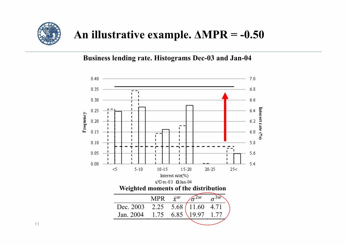
An illustrative example. ΔMPR = -0.50

Business lending rate. Histograms Dec-03 and Jan-04

8



9

Inspired by the financial literature: Higher order moments as measures of credit risk

Variance: Higher variance, higher uncertaintyof the client portfolio, higher credit riskpremium, higher interest rate. Expected effecton the rate: +

Skewness: More negative skewness, thedistribution moves to the right, more higher-risks clients, higher interest rate. Expectedeffect on the rate: -

[High correlation with kurtosis]

Observable: Interest rate, which includescredit risk premium.

10



Weighted moments of the distribution MPR ̅ 2 3

Dec. 2003 2.25 5.68 11.60 4.71Jan. 2004 1.75 6.85 19.97 1.77

11



Weighted moments of the distribution MPR ̅ 2 3

Dec. 2003 2.25 5.68 11.60 4.71Jan. 2004 1.75 6.85 19.97 1.77

12

Related literature: MPR pass-through in Chile

Espinosa-Vega & Rebucci (2004, CBC book): Pass-throughin Chile is similar to those in other countries, butincomplete in the long run.

Econometric model: Error-Correction ADL. Interest rates ofconsumption and business loans, in pesos and CPI-indexed(UF).

April 1993 – September 2002.

Becerra et al. (2010, Chilean Economy): The lack of pass-through during the financial crisis can be explained byhigher national and international risk.

Econometric model: ADL. Nominal interest rates ofconsumption and business loans.

2005-2009, weekly observations.

13

Related literature: The risk-taking Channel

The risk-taking Channel: Low interest rates makecommercial banks take higher risk on loans.

Adrian & Liang (2014, Staff Report FEDNY): Overview ofstudies on the risk-taking channel.

Jiménez et al. (2014, Econometrica): What do 23 millionsbank loans tell about the effect of the monetary policy on thecredit risk taken by commercial banks?

Commercial banks take higher credit risks when the MPR islow.

A study of applications and loan contracts.

This study: Is there an easier way to measure credit risk?

14

A simple framework to illustrate the context in which the empirical study is conducted

Let r be the return on a 1 dollar loan.

To simplify, assume perfect competition, risk neutral banks, zero recuperationrate and no arbitrage in prices. Let p be the default probability and rf the risk-freeinterest rate. Then:

(1 + r)(1 – p) + 0p = 1 + E(r) = 1 + rf

1 + r = (1 + rf) / (1 – p)

r ≈ rf + p

Hence, with a one-to-one relationship between the MPR and the risk-free interestrate, the pass-through is instantaneous and complete when adjusting by the creditrisk.

In line with Merton (1974).

15

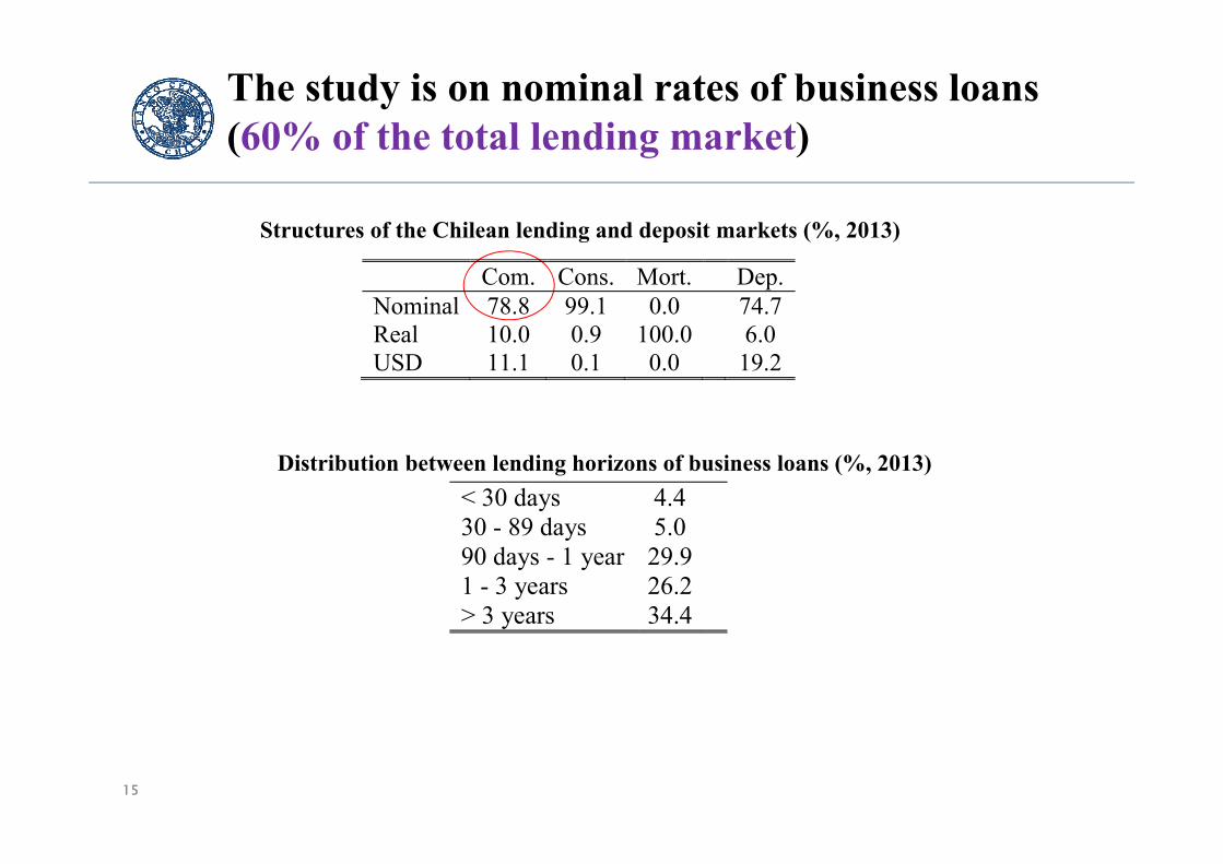
The study is on nominal rates of business loans (60% of the total lending market)

Structures of the Chilean lending and deposit markets (%, 2013)

Com. Cons. Mort. Dep.Nominal 78.8 99.1 0.0 74.7 Real 10.0 0.9 100.0 6.0 USD 11.1 0.1 0.0 19.2

Distribution between lending horizons of business loans (%, 2013)< 30 days 4.4 30 - 89 days 5.0 90 days - 1 year 29.9 1 - 3 years 26.2 > 3 years 34.4

16

The study is on nominal rates of business loans (60% of the total lending market)

Structures of the Chilean lending and deposit markets (%, 2013)

Com. Cons. Mort. Dep.Nominal 78.8 99.1 0.0 74.7 Real 10.0 0.9 100.0 6.0 USD 11.1 0.1 0.0 19.2

Distribution between lending horizons of business loans (%, 2013)< 30 days 4.4 30 - 89 days 5.0 90 days - 1 year 29.9 1 - 3 years 26.2 > 3 years 34.4

17

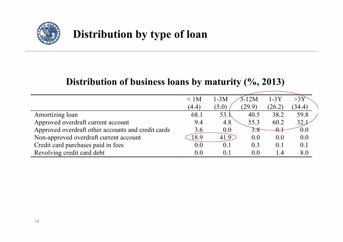
Distribution by type of loan

Distribution of business loans by maturity (%, 2013)

< 1M 1-3M 3-12M 1-3Y >3Y (4.4) (5.0) (29.9) (26.2) (34.4)

Amortizing loan 68.1 53.1 40.5 38.2 59.8 Approved overdraft current account 9.4 4.8 55.3 60.2 32.1 Approved overdraft other accounts and credit cards 3.6 0.0 3.8 0.1 0.0 Non-approved overdraft current account 18.9 41.9 0.0 0.0 0.0 Credit card purchases paid in fees 0.0 0.1 0.3 0.1 0.1 Revolving credit card debt 0.0 0.1 0.0 1.4 8.0

18

Distribution by type of loan

< 1M 1-3M 3-12M 1-3Y >3Y (4.4) (5.0) (29.9) (26.2) (34.4)

Amortizing loan 68.1 53.1 40.5 38.2 59.8 Approved overdraft current account 9.4 4.8 55.3 60.2 32.1 Approved overdraft other accounts and credit cards 3.6 0.0 3.8 0.1 0.0 Non-approved overdraft current account 18.9 41.9 0.0 0.0 0.0 Credit card purchases paid in fees 0.0 0.1 0.3 0.1 0.1 Revolving credit card debt 0.0 0.1 0.0 1.4 8.0

Distribution of business loans by maturity (%, 2013)

19

Data: Commercial Interest rates and risk measures

Variable of interest: Monthly business interest rate: ijt (j = 0,1,2,3)

Period: Jan.02 – Feb.17 (t = 1,…,182)

Daily interest rates for each bank are utilized to calculate weighted moments forintra policy meetings periods:

1,

1,

j: loan type (0: total, 1: 3-12M, 2: 1-3Y, 3: >3Y)

d: day of operation, d = 1,…,Djt

b: bank: b = 1,…,Bjt

ωj: Amount of the loan with interest rate ij

σkw(ijt): weighted k’th moment of the distribution with weighted mean ijt.

20

Interest rate and risk measures

σ2w(ijt) σ3w(ijt)

i0t

i1t

i2t

i3t

012345678910

05

101520253035404550

2002 2004 2006 2008 2010 2012 2014 2016

Correlation: 0.70

012345678910

0.00.51.01.52.02.53.03.54.04.55.0

2002 2004 2006 2008 2010 2012 2014 2016

Correlation: -0.73

0

2

4

6

8

10

12

05

101520253035404550

2002 2004 2006 2008 2010 2012 2014 2016

Correlation: 0.55

0

2

4

6

8

10

12

0.0

0.5

1.0

1.5

2.0

2.5

3.0

3.5

4.0

2002 2004 2006 2008 2010 2012 2014 2016

Correlation: -0.79

0

5

10

15

20

25

0

50

100

150

200

250

2002 2004 2006 2008 2010 2012 2014 2016

Correlation: 0.73

0

5

10

15

20

25

-2-1012345678

2002 2004 2006 2008 2010 2012 2014 2016

Correlation: -0.74

0

2

4

6

8

10

12

14

16

18

0102030405060708090

100

2002 2004 2006 2008 2010 2012 2014 2016

Correlation: 0.10

0

2

4

6

8

10

12

14

16

18

-1

0

1

2

3

4

5

6

7

8

2002 2004 2006 2008 2010 2012 2014 2016

Correlation: -0.80

Risk measures (solid, LHS) and difference between commercial and interbank interest rates (punctuated, RHS)

21

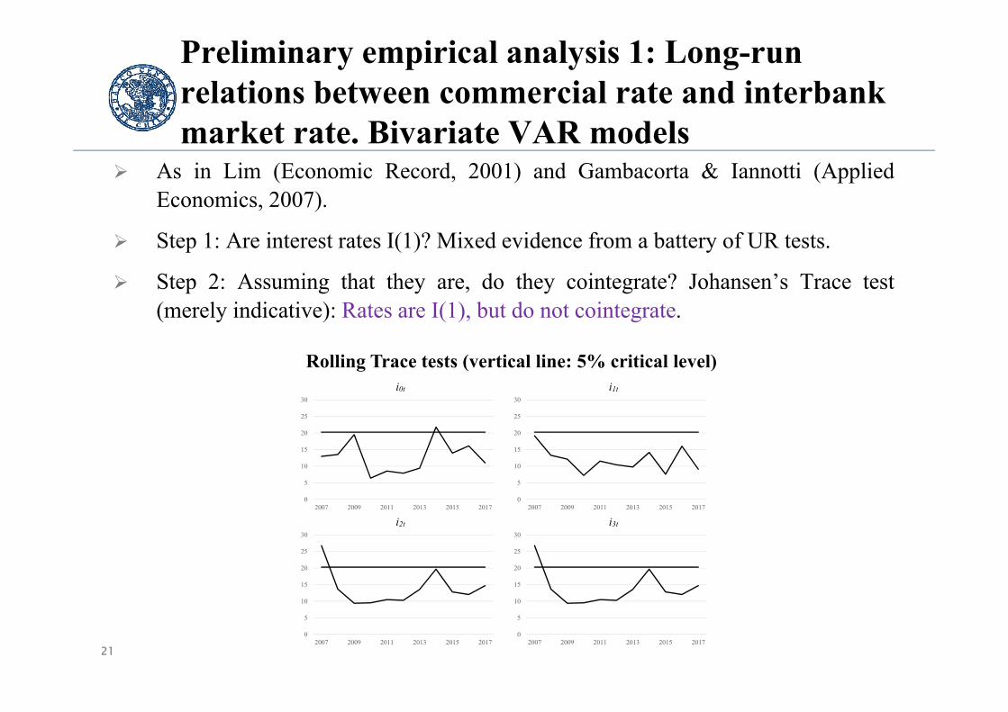
Preliminary empirical analysis 1: Long-run relations between commercial rate and interbank market rate. Bivariate VAR models

As in Lim (Economic Record, 2001) and Gambacorta & Iannotti (AppliedEconomics, 2007).

Step 1: Are interest rates I(1)? Mixed evidence from a battery of UR tests.

Step 2: Assuming that they are, do they cointegrate? Johansen’s Trace test(merely indicative): Rates are I(1), but do not cointegrate.

i0t i1t

i2t i3t

0

5

10

15

20

25

30

2007 2009 2011 2013 2015 20170

5

10

15

20

25

30

2007 2009 2011 2013 2015 2017

0

5

10

15

20

25

30

2007 2009 2011 2013 2015 20170

5

10

15

20

25

30

2007 2009 2011 2013 2015 2017

Rolling Trace tests (vertical line: 5% critical level)

22

Preliminary empirical analysis 2: Long-run relations between interest rates and risk measures. 4-dimensional VAR models

Include risk measure in VAR models

Step 1: Are risk measures I(1)? Mixed evidence from a battery of UR tests.

Step 2: Assuming that they are, do they cointegrate with the interest rates?Johansen’s Trace test (merely indicative): Variables are I(1), but do notcointegrate.

Rolling Trace tests (vertical line: 5% critical level)i0t i1t

i2t i3t

0

10

2030

4050

60

7080

90

2007 2009 2011 2013 2015 20170

10

20

30

40

50

60

70

2007 2009 2011 2013 2015 2017

0

10

2030

4050

60

7080

90

2007 2009 2011 2013 2015 20170

10

2030

4050

60

7080

90

2007 2009 2011 2013 2015 2017

23

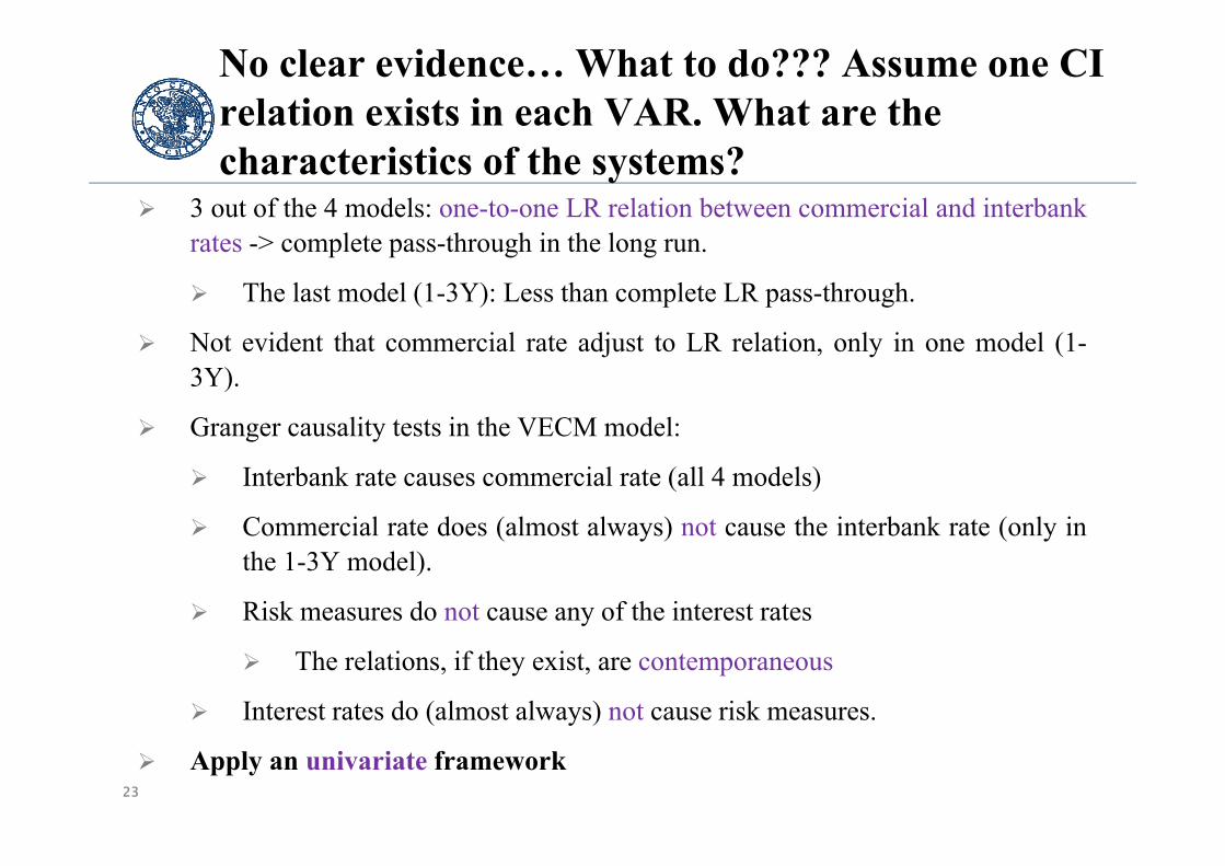
No clear evidence… What to do??? Assume one CI relation exists in each VAR. What are the characteristics of the systems?

3 out of the 4 models: one-to-one LR relation between commercial and interbankrates -> complete pass-through in the long run.

The last model (1-3Y): Less than complete LR pass-through.

Not evident that commercial rate adjust to LR relation, only in one model (1-3Y).

Granger causality tests in the VECM model:

Interbank rate causes commercial rate (all 4 models)

Commercial rate does (almost always) not cause the interbank rate (only inthe 1-3Y model).

Risk measures do not cause any of the interest rates

The relations, if they exist, are contemporaneous

Interest rates do (almost always) not cause risk measures.

Apply an univariate framework

24

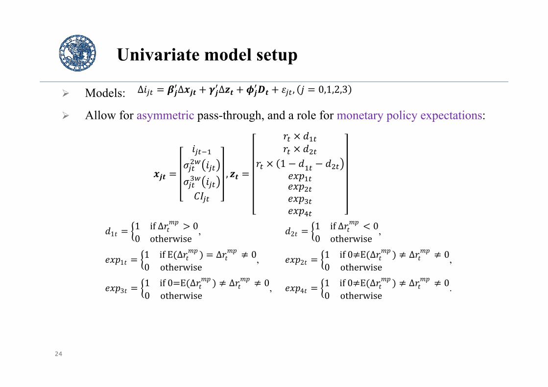
Univariate model setup

Models:

Allow for asymmetric pass-through, and a role for monetary policy expectations:

11 ifΔ 00 otherwise

, 21 if Δ 00 otherwise

,

11 ifE Δ Δ 00 otherwise

, 21 if0 E Δ Δ 00 otherwise

,

31 if0 E Δ Δ 00 otherwise

, 41 if0 E Δ Δ 00 otherwise

.

,1

∆ ∆ ∆ , 0,1,2,3

25

Univariate model setup (cont.)

Deterministic terms: constant, seasonal and outlier dummies.

Method: General-to-specific, i.e. based on inference.

Problems:

Auto correlated residuals:

Solution: Include MA-terms in the residuals

Relatively small sample (65 changes of the policy rate)

Solution: Standard errors estimated with jackknife replications.

Robustness estimations:

Business cycle, inflation rate, national and international general risk measures(EMBI and VIX), and a measure of non-conventional monetary policy are notimportant variables.

Credit risk and interest rate interaction terms are mostly not statisticallysignificant and do not affect the presented estimated coefficients.

26

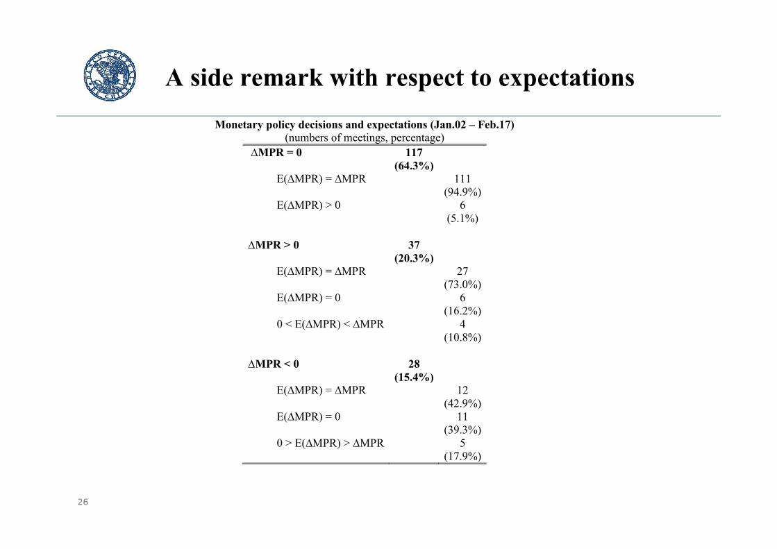
A side remark with respect to expectations

Monetary policy decisions and expectations (Jan.02 – Feb.17) (numbers of meetings, percentage)

∆MPR = 0 117 (64.3%)

E(∆MPR) = ∆MPR 111 (94.9%)

E(∆MPR) > 0 6 (5.1%)

∆MPR > 0 37

(20.3%)

E(∆MPR) = ∆MPR 27 (73.0%)

E(∆MPR) = 0 6 (16.2%)

0 < E(∆MPR) < ∆MPR 4 (10.8%)

∆MPR < 0 28

(15.4%)

E(∆MPR) = ∆MPR 12 (42.9%)

E(∆MPR) = 0 11 (39.3%)

0 > E(∆MPR) > ∆MPR 5 (17.9%)

27

Results of estimations

Estimations results. Dependent variable: Change in business lending rate Δi0t Δi1t Δi2t Δi3t Const. -0.01

(0.01) -0.01*

(0.01) -0.02 (0.02)

-0.02 (0.03)

-0.01 (0.05)

-0.05(0.04)

0.05 (0.05)

-0.04 (0.05)

∆ 1 0.23***

(0.08) 0.24***

(0.08) 0.01(0.37)

0.03(0.23)

0.01

(0.06) 0.02(0.04)

-0.03(0.04)

0.04(0.04)

∆ 1 1.01***

(0.38) 0.93***

(0.15) 2.10**

(1.00) 1.19**

(0.47) 1.76

(1.95) 1.25***

(0.41) 1.91(1.28)

1.46**

(0.68) ∆ 2 0.73***

(0.24) 0.77***

(0.18) 0.47 (0.34)

0.82*** (0.27)

0.58 (0.91)

0.66 (0.78)

0.71 (0.52)

0.87**

(0.41) ∆ 1 1 2 -0.10

(0.59) -0.96

(1.60) 0.27

(3.91) -5.42

(3.28)

1 -0.01(0.02)

-0.08(0.15)

-0.09

(0.12) -0.05*

(0.03)

∆ 2 0.07***

(0.005) 0.07***

(0.01) 0.06***

(0.01) 0.06***

(0.01) 0.05***

(0.005) 0.05***

(0.004) -0.004 (0.007)

∆ 3 -0.47***

(0.08) -0.47***

(0.09) -0.59***

(0.21) -0.56**

(0.23) -1.69***

(0.13) -1.68***

(0.15) -2.75***

(0.14) -2.61***

(0.11)

1 -0.04(0.11)

-0.26*

(0.16) -0.22

(0.59) -0.25

(0.42)

2 -0.07(0.24)

-0.61 (0.37)

-0.31 (1.34)

-0.31 (0.92)

3 0.02(0.13)

-0.08 (0.48)

-0.25 (0.50)

-0.55 (0.41)

4 0.16(0.13)

0.21(0.26)

0.54 (0.70)

0.43 (0.52)

Observations 181 181 181 181 181 181 181 181 2 0.77 0.78 0.54 0.52 0.86 0.87 0.73 0.72

LogL 4.70 -0.64 -104.6 -112.1 -210.2 -212.2 -289.7 -296.4 Wald 0.93 0.15 0.98 0.09 LR 0.87 0.08 0.69 0.06 LM 0.02 0.06 0.04 0.99

Notes: Numbers in parentheses are jackknife estimated standard errors. */**/***: Statistically significant whapplying a 10%/5%/1% confidence level. LogL: Value of maximized log likelihood function. Wald / LR / LM:value of Wald / Lagrange ratio / Lagrange multiplier test for the restrictions imposed.

28

Result 1: Expectations are not important


(0.01) -0.01*

(0.01) -0.02 (0.02)

-0.02 (0.03)

-0.01 (0.05)

-0.05(0.04)

0.05 (0.05)

-0.04 (0.05)

∆ 1 0.23***

(0.08) 0.24***

(0.08) 0.01(0.37)

0.03(0.23)

0.01

(0.06) 0.02(0.04)

-0.03(0.04)

0.04(0.04)

∆ 1 1.01***

(0.38) 0.93***

(0.15) 2.10**

(1.00) 1.19**

(0.47) 1.76

(1.95) 1.25***

(0.41) 1.91(1.28)

1.46**

(0.68) ∆ 2 0.73***

(0.24) 0.77***

(0.18) 0.47 (0.34)

0.82*** (0.27)

0.58 (0.91)

0.66 (0.78)

0.71 (0.52)

0.87**

(0.41) ∆ 1 1 2 -0.10

(0.59) -0.96

(1.60) 0.27

(3.91) -5.42

(3.28)

1 -0.01(0.02)

-0.08(0.15)

-0.09

(0.12) -0.05*

(0.03)

∆ 2 0.07***

(0.005) 0.07***

(0.01) 0.06***

(0.01) 0.06***

(0.01) 0.05***

(0.005) 0.05***

(0.004) -0.004 (0.007)

∆ 3 -0.47***

(0.08) -0.47***

(0.09) -0.59***

(0.21) -0.56**

(0.23) -1.69***

(0.13) -1.68***

(0.15) -2.75***

(0.14) -2.61***

(0.11)

1 -0.04(0.11)

-0.26*

(0.16) -0.22

(0.59) -0.25

(0.42)

2 -0.07(0.24)

-0.61 (0.37)

-0.31 (1.34)

-0.31 (0.92)

3 0.02(0.13)

-0.08 (0.48)

-0.25 (0.50)

-0.55 (0.41)

4 0.16(0.13)

0.21(0.26)

0.54 (0.70)

0.43 (0.52)

Observations 181 181 181 181 181 181 181 181 2 0.77 0.78 0.54 0.52 0.86 0.87 0.73 0.72

LogL 4.70 -0.64 -104.6 -112.1 -210.2 -212.2 -289.7 -296.4 Wald 0.93 0.15 0.98 0.09 LR 0.87 0.08 0.69 0.06 LM 0.02 0.06 0.04 0.99


29

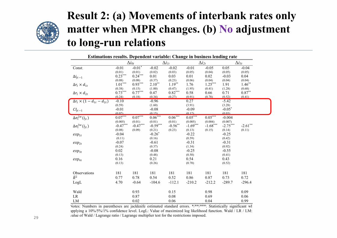
Result 2: (a) Movements of interbank rates only matter when MPR changes. (b) No adjustment to long-run relations


(0.01) -0.01*

(0.01) -0.02 (0.02)

-0.02 (0.03)

-0.01 (0.05)

-0.05(0.04)

0.05 (0.05)

-0.04 (0.05)

∆ 1 0.23***

(0.08) 0.24***

(0.08) 0.01(0.37)

0.03(0.23)

0.01

(0.06) 0.02(0.04)

-0.03(0.04)

0.04(0.04)

∆ 1 1.01***

(0.38) 0.93***

(0.15) 2.10**

(1.00) 1.19**

(0.47) 1.76

(1.95) 1.25***

(0.41) 1.91(1.28)

1.46**

(0.68) ∆ 2 0.73***

(0.24) 0.77***

(0.18) 0.47 (0.34)

0.82*** (0.27)

0.58 (0.91)

0.66 (0.78)

0.71 (0.52)

0.87**

(0.41) ∆ 1 1 2 -0.10

(0.59) -0.96

(1.60) 0.27

(3.91) -5.42

(3.28)

1 -0.01(0.02)

-0.08(0.15)

-0.09

(0.12) -0.05*

(0.03)

∆ 2 0.07***

(0.005) 0.07***

(0.01) 0.06***

(0.01) 0.06***

(0.01) 0.05***

(0.005) 0.05***

(0.004) -0.004 (0.007)

∆ 3 -0.47***

(0.08) -0.47***

(0.09) -0.59***

(0.21) -0.56**

(0.23) -1.69***

(0.13) -1.68***

(0.15) -2.75***

(0.14) -2.61***

(0.11)

1 -0.04(0.11)

-0.26*

(0.16) -0.22

(0.59) -0.25

(0.42)

2 -0.07(0.24)

-0.61 (0.37)

-0.31 (1.34)

-0.31 (0.92)

3 0.02(0.13)

-0.08 (0.48)

-0.25 (0.50)

-0.55 (0.41)

4 0.16(0.13)

0.21(0.26)

0.54 (0.70)

0.43 (0.52)

Observations 181 181 181 181 181 181 181 181 2 0.77 0.78 0.54 0.52 0.86 0.87 0.73 0.72

LogL 4.70 -0.64 -104.6 -112.1 -210.2 -212.2 -289.7 -296.4 Wald 0.93 0.15 0.98 0.09 LR 0.87 0.08 0.69 0.06 LM 0.02 0.06 0.04 0.99


30

Result 3: Credit risk measures matter and with the expected signs


(0.01) -0.01*

(0.01) -0.02 (0.02)

-0.02 (0.03)

-0.01 (0.05)

-0.05(0.04)

0.05 (0.05)

-0.04 (0.05)

∆ 1 0.23***

(0.08) 0.24***

(0.08) 0.01(0.37)

0.03(0.23)

0.01

(0.06) 0.02(0.04)

-0.03(0.04)

0.04(0.04)

∆ 1 1.01***

(0.38) 0.93***

(0.15) 2.10**

(1.00) 1.19**

(0.47) 1.76

(1.95) 1.25***

(0.41) 1.91(1.28)

1.46**

(0.68) ∆ 2 0.73***

(0.24) 0.77***

(0.18) 0.47 (0.34)

0.82*** (0.27)

0.58 (0.91)

0.66 (0.78)

0.71 (0.52)

0.87**

(0.41) ∆ 1 1 2 -0.10

(0.59) -0.96

(1.60) 0.27

(3.91) -5.42

(3.28)

1 -0.01(0.02)

-0.08(0.15)

-0.09

(0.12) -0.05*

(0.03)

∆ 2 0.07***

(0.005) 0.07***

(0.01) 0.06***

(0.01) 0.06***

(0.01) 0.05***

(0.005) 0.05***

(0.004) -0.004 (0.007)

∆ 3 -0.47***

(0.08) -0.47***

(0.09) -0.59***

(0.21) -0.56**

(0.23) -1.69***

(0.13) -1.68***

(0.15) -2.75***

(0.14) -2.61***

(0.11)

1 -0.04(0.11)

-0.26*

(0.16) -0.22

(0.59) -0.25

(0.42)

2 -0.07(0.24)

-0.61 (0.37)

-0.31 (1.34)

-0.31 (0.92)

3 0.02(0.13)

-0.08 (0.48)

-0.25 (0.50)

-0.55 (0.41)

4 0.16(0.13)

0.21(0.26)

0.54 (0.70)

0.43 (0.52)

Observations 181 181 181 181 181 181 181 181 2 0.77 0.78 0.54 0.52 0.86 0.87 0.73 0.72

LogL 4.70 -0.64 -104.6 -112.1 -210.2 -212.2 -289.7 -296.4 Wald 0.93 0.15 0.98 0.09 LR 0.87 0.08 0.69 0.06 LM 0.02 0.06 0.04 0.99


31

Result 4: When controlling for changes in the credit risk, MPR pass-through cannot be rejected to be symmetric and instantaneously complete


(0.01) -0.01*

(0.01) -0.02 (0.02)

-0.02 (0.03)

-0.01 (0.05)

-0.05(0.04)

0.05 (0.05)

-0.04 (0.05)

∆ 1 0.23***

(0.08) 0.24***

(0.08) 0.01(0.37)

0.03(0.23)

0.01

(0.06) 0.02(0.04)

-0.03(0.04)

0.04(0.04)

∆ 1 1.01***

(0.38) 0.93***

(0.15) 2.10**

(1.00) 1.19**

(0.47) 1.76

(1.95) 1.25***

(0.41) 1.91(1.28)

1.46**

(0.68) ∆ 2 0.73***

(0.24) 0.77***

(0.18) 0.47 (0.34)

0.82*** (0.27)

0.58 (0.91)

0.66 (0.78)

0.71 (0.52)

0.87**

(0.41) ∆ 1 1 2 -0.10

(0.59) -0.96

(1.60) 0.27

(3.91) -5.42

(3.28)

1 -0.01(0.02)

-0.08(0.15)

-0.09

(0.12) -0.05*

(0.03)

∆ 2 0.07***

(0.005) 0.07***

(0.01) 0.06***

(0.01) 0.06***

(0.01) 0.05***

(0.005) 0.05***

(0.004) -0.004 (0.007)

∆ 3 -0.47***

(0.08) -0.47***

(0.09) -0.59***

(0.21) -0.56**

(0.23) -1.69***

(0.13) -1.68***

(0.15) -2.75***

(0.14) -2.61***

(0.11)

1 -0.04(0.11)

-0.26*

(0.16) -0.22

(0.59) -0.25

(0.42)

2 -0.07(0.24)

-0.61 (0.37)

-0.31 (1.34)

-0.31 (0.92)

3 0.02(0.13)

-0.08 (0.48)

-0.25 (0.50)

-0.55 (0.41)

4 0.16(0.13)

0.21(0.26)

0.54 (0.70)

0.43 (0.52)

Observations 181 181 181 181 181 181 181 181 2 0.77 0.78 0.54 0.52 0.86 0.87 0.73 0.72

LogL 4.70 -0.64 -104.6 -112.1 -210.2 -212.2 -289.7 -296.4 Wald 0.93 0.15 0.98 0.09 LR 0.87 0.08 0.69 0.06 LM 0.02 0.06 0.04 0.99


32

Result 4: When controlling for changes in the credit risk, MPR pass-through cannot be rejected to be symmetric and instantaneously complete


(0.01) -0.01*

(0.01) -0.02 (0.02)

-0.02 (0.03)

-0.01 (0.05)

-0.05(0.04)

0.05 (0.05)

-0.04 (0.05)

∆ 1 0.23***

(0.08) 0.24***

(0.08) 0.01(0.37)

0.03(0.23)

0.01

(0.06) 0.02(0.04)

-0.03(0.04)

0.04(0.04)

∆ 1 1.01***

(0.38) 0.93***

(0.15) 2.10**

(1.00) 1.19**

(0.47) 1.76

(1.95) 1.25***

(0.41) 1.91(1.28)

1.46**

(0.68) ∆ 2 0.73***

(0.24) 0.77***

(0.18) 0.47 (0.34)

0.82*** (0.27)

0.58 (0.91)

0.66 (0.78)

0.71 (0.52)

0.87**

(0.41) ∆ 1 1 2 -0.10

(0.59) -0.96

(1.60) 0.27

(3.91) -5.42

(3.28)

1 -0.01(0.02)

-0.08(0.15)

-0.09

(0.12) -0.05*

(0.03)

∆ 2 0.07***

(0.005) 0.07***

(0.01) 0.06***

(0.01) 0.06***

(0.01) 0.05***

(0.005) 0.05***

(0.004) -0.004 (0.007)

∆ 3 -0.47***

(0.08) -0.47***

(0.09) -0.59***

(0.21) -0.56**

(0.23) -1.69***

(0.13) -1.68***

(0.15) -2.75***

(0.14) -2.61***

(0.11)

1 -0.04(0.11)

-0.26*

(0.16) -0.22

(0.59) -0.25

(0.42)

2 -0.07(0.24)

-0.61 (0.37)

-0.31 (1.34)

-0.31 (0.92)

3 0.02(0.13)

-0.08 (0.48)

-0.25 (0.50)

-0.55 (0.41)

4 0.16(0.13)

0.21(0.26)

0.54 (0.70)

0.43 (0.52)

Observations 181 181 181 181 181 181 181 181 2 0.77 0.78 0.54 0.52 0.86 0.87 0.73 0.72

LogL 4.70 -0.64 -104.6 -112.1 -210.2 -212.2 -289.7 -296.4 Wald 0.93 0.15 0.98 0.09 LR 0.87 0.08 0.69 0.06 LM 0.02 0.06 0.04 0.99


p-values for the hypotheses of symmetric and instantaneously complete pass-through:

0.42, 0.65, 0.75, 0.79.

33

Conclusions and policy recommendations

The information in the weighted average of a commercial interest rate may belimited. Higher order moments help with a more complete vision.

Changes in the higher order moments supply information about changes in therisk associated with the portfolio of clients.

In a theoretical illustrations it can be shown that with a one-to-one relationbetween the risk-free interest rate and the monetary policy rate (MPR), the pass-through of MPR changes is instantaneous and complete when correcting forchanges in the credit risk.

Empirical estimations confirm this relation in Chile.

Policy recommendations:

To better understand changes in commercial interest rates, not only theweighted averages of the rates should be monitored, but also the higherorder moments of the distribution. This is particularly important whenevaluating the effects of MPR changes.

For transparency: Publish these higher order moments.

Credit Risk and Monetary Pass-through. Evidence from Chile

Economy & Finance

Transcript of Credit Risk and Monetary Pass-through. Evidence from Chile