NEPI Working Paper

Consequences of U.S. Dependence on Foreign Oil

Stephen P. A. Brown and Ryan T. Kennelly

April 4, 2013

2  

Consequences of U.S. Dependence on Foreign Oil  

Stephen P. A. Brown and Ryan T. Kennelly* Center for Business and Economic Research 

University of Nevada, Las Vegas  

April 4, 2013  Overview We examine the consequences of U.S. dependence on foreign oil.  We use an encompassing approach that includes many ideas about the costs arising from U.S. dependence on foreign oil, but we identify which ideas have broad support in the economics literature and which ideas have limited support.  Consistent with our approach, we quantify the costs of U.S. dependence on foreign oil using a relatively broad metric that is based in a long‐standing economics literature and a relatively narrow metric that is confined to oil‐security externalities as defined by Brown and Huntington (2013).  We estimate these costs from 2010 through 2035 by taking into account projected world oil market conditions, the exercise of market power, probable oil supply disruptions, the market response to oil supply disruptions, and the resulting U.S. economic losses.  1. Introduction 

Since the comprehensive study of energy markets carried out by Landsberg et al. (1979), 

economists and other analysts have recognized that U.S. dependence on imported oil is likely to yield a 

variety of social costs in excess of the market price paid for the oil.  In addition to the well‐recognized 

environmental costs associated with the consumption of domestic or imported oil, other costs resulting 

from U.S. dependence on imported oil may include such elements as the macroeconomic risks 

associated with greater exposure to world oil supply disruptions, the foregone opportunities for the 

United States to exercise market power in the world oil market, the costs to the United States of 

maintaining a strong military presence in the Middle East, and various factors affecting foreign policy. 

                                                           * Stephen P. A. Brown is Professor of Economics and Director of the Center for Business and Economic Research at the University of Nevada, Las Vegas.  Ryan T. Kennelly is Economic Analyst at the Center for Business and Economic Research at the University of Nevada, Las Vegas.  The authors wish to thank Mary Haddican, Hill Huntington, Tony Knowles, André Plourde and David Victor for helpful discussions and comments; Kylelar Maravich for capable research assistance; and Rennae Daneshvary and Mary Haddican for editing. 

3  

Over the years, researchers have produced numerous and conflicting approaches to assessing 

the costs of U.S. dependence on foreign oil.  These approaches include an oil import premium, an oil 

security premium, an assessment of the costs of achieving oil independence, an evaluation of the 

political costs of U.S. dependence on foreign oil, and a denial that any such costs can be regarded as 

externalities that require a policy response.  

Landsberg et al. (1979) developed an oil import premium that relied on quantifying two 

elements: 1) the increased size of the expected losses (in the form of the macroeconomic disruptions 

and transfers resulting from world oil price shocks) associated with increased reliance on imported oil; 

and 2) the ability of the U.S. government to exercise market power by reducing U.S. oil imports to 

reduce world oil prices.  Subsequent work in this vein includes Bohi and Montgomery (1982a, 1982b), 

Brown (1982), Broadman (1986), Bohi and Toman (1993), Toman (1993), Parry and Darmstadter (2003), 

and Leiby (2007).  Some of this literature has estimated premiums at prevailing or projected world oil 

market conditions.  Some of the literature has estimated optimal oil import premiums.1 

Brown and Huntington (2013) narrow inquiry from the dominant approach by estimating an oil 

security premium.  They identify the oil security premium as the expected transfers and macroeconomic 

losses associated with disruptions that interrupt the flow of oil consumption.  Following mainstream 

economics literature, they argue that the failure of the United States to exercise its market power in the 

world oil market does not represent a true economic externality.  Using energy market conditions 

projected by the U.S. Energy Information Administration (EIA), Brown and Huntington estimate oil 

security premiums associated with the consumption of domestic and imported oil.  They find relatively 

small oil security premiums, with somewhat larger premiums for imported oil rather than domestic oil. 

                                                           1 The optimal oil import premium is calculated for the change in world oil market conditions that would occur were the premium implemented as a tax.  In general, the optimal premium is lower than the premium at prevailing market conditions, because implementation of the premium as a tax reduces U.S. imports and the world oil price. 

4  

The National Research Council (2009) goes farther than Brown and Huntington and argues that 

the non‐environmental externalities associated with U.S. dependence on foreign oil are extremely small 

or nonexistent.  The council’s analysis consists of carefully defining what is meant by externality and 

then proceeds to reject the arguments made in previous analyses for regarding the costs of dependence 

on foreign oil as externalities.  The council’s conclusions are at odds with other economics literature, 

such as John (1995) and Huntington (2003) who provide evidence that the macroeconomic losses ought 

to be considered externalities. 

Greene et al. (2007) and Greene (2010, 2011) estimate the costs of achieving U.S. oil 

independence.  To set a standard for independence, these exercises recognize that independence does 

not require reducing oil imports to zero.  Rather, it requires reducing dependence to a manageable level.  

According to Greene (2010), the first step in determining a manageable level is to estimate the total 

costs of U.S. oil dependence, using elements that are similar to those described above.  According to 

Greene (2011), sufficient independence is achieved by reducing imports so that these expected costs are 

reduced to 1 percent of GDP.  This standard is set without any attempt to balance costs and benefits. 

In a substantial departure from the economics literature, the Council on Foreign Relations 

(2006) identified six costs of U.S. dependence on imported oil: 1) Significant interruptions in oil supply 

will have adverse political and economic consequences in the United States and other importing 

countries; 2) High prices and seemingly scarce supplies create fears that the current system of open 

markets is unable to ensure secure supply; 3) Control over oil revenues gives exporting countries the 

flexibility to adopt policies that oppose U.S. interests and values; 4) Oil dependence causes political 

realignments that constrain the ability of the United States to form alliances and partnerships to achieve 

common objectives; 5) Revenues from oil and gas exports can undermine local governance; and 6) If the 

U.S. reduced its dependence on oil, it would not have as great an interest in the Middle East and could 

reduce its military posture there. 

5  

The Council on Foreign Relations study is best understood as a consensus‐building exercise to 

examine the political implications of U.S. dependence on imported oil.  As such, it offered no thoughts 

about quantifying the costs it identified.  In another departure from the mainstream of economic 

thinking, however, Hall (1992, 2004) offers estimates of the costs of defense spending and the strategic 

petroleum reserve as a way to measure the costs of U.S. dependence on imported oil. 

In the present exercise, we undertake a variety of tasks to further understanding of the costs of 

U.S. reliance on imported oil.  In section 2, we sort through the various ideas about how to evaluate the 

costs of U.S. dependence on imported and domestically produced oil.  In section 3, we consolidate these 

measures and use them to quantify the costs of U.S. dependence on foreign oil under five different 

world oil market scenarios taken or adapted from the EIA’s 2012 Annual Energy Outlook.  Section 4 

examines the implications of using the estimated costs as a guide to policy.  Section 5 concludes by 

considering the policy options. 

2. Understanding the Consequences of U.S. Dependence on Oil Imports 

  Previous research and analysis have suggested a number of possible costs associated with U.S. 

dependence on foreign oil.  These costs include U.S. reliance on oil produced in a world oil market that is 

dominated by a cartel that exercises monopoly power, expected economic losses associated with supply 

disruptions, fears that a free market cannot ensure a secure supply, increases in government spending 

to reduce the vulnerability of supply, the limits that oil imports place on U.S. foreign policy, the effect of 

oil dependence on international alliances, the uses to which some oil‐exporting countries put their 

revenue, and the ability of oil revenue to undermine local governance.  The list is long, but not all of 

these costs represent what economists would consider market failures.  The distinction is important 

because economists generally consider market failure as the only compelling reason for a policy 

response.   

6  

Externalities are one type of market failure.  They arise when a market transaction imposes 

costs or risks on an individual who is not party to the transaction.  Another type of market failure occurs 

when the exercise of monopoly power causes market prices to be much higher than production costs.  

Both such market failures are frequently cited as a reason for the United States to reduce its 

dependence on foreign oil. 

  To explore these issues, we develop a welfare‐analytic model of U.S. oil consumption and use it 

as a springboard to examine whether each of nine different costs of U.S. reliance on imported oil ought 

to be considered potential market failures and can be quantified.  In doing so, we take two approaches.  

We take a broad approach that contains all of the quantifiable costs that have been identified in the oil 

import literature that begins with Landsberg et al. (1979) and continues through to Greene (2011).  We 

also take a narrow approach and include only those costs which Brown and Huntington (2013) regard as 

the security externalities associated with the consumption of imported oil. 

2.1. Welfare Analytics of U.S. Oil Consumption, Imports, and Production 

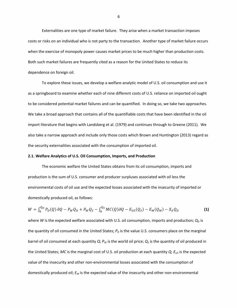
The economic welfare the United States obtains from its oil consumption, imports and 

production is the sum of U.S. consumer and producer surpluses associated with oil less the 

environmental costs of oil use and the expected losses associated with the insecurity of imported or 

domestically produced oil, as follows:  

𝑊 = ∫ 𝑃%(𝑄))*+ 𝜕𝑄 − 𝑃.𝑄% + 𝑃.𝑄0 − ∫ 𝑀𝐶(𝑄)𝜕𝑄)3

+ − 𝐸50(𝑄0) − 𝐸6(𝑄6) − 𝑋8𝑄%             (1) 

where W is the expected welfare associated with U.S. oil consumption, imports and production; QD is 

the quantity of oil consumed in the United States; PD is the value U.S. consumers place on the marginal 

barrel of oil consumed at each quantity Q; PW is the world oil price; QS is the quantity of oil produced in 

the United States; MC is the marginal cost of U.S. oil production at each quantity Q; EUS is the expected 

value of the insecurity and other non‐environmental losses associated with the consumption of 

domestically produced oil; EM is the expected value of the insecurity and other non‐environmental 

7  

losses associated with the consumption of imported oil; QM is the quantity of imported oil; and XE is the 

economic value of environmental externalities associated with U.S. oil consumption.  According to our 

welfare‐analytic approach, the total well being that the United States gains from its oil consumption, 

imports and production can be measured by the benefits received by consumers from using the oil in 

excess of what they pay for the oil, the revenue received by the domestic oil producers less their 

production costs, minus the environmental costs associated with oil use and the expected losses 

associated with oil insecurity.  

  For the consumption of domestically produced oil, the optimality condition is 

𝑃% = 𝑀𝐶)9 +:8;3:)3

+ 𝑋8.                           (2) 

The optimal use of domestic oil occurs when the domestic oil price is equal to the marginal cost of 

domestic production plus the change in expected insecurity and other non‐environmental costs 

associated with additional consumption of domestic oil and the value of environmental externalities 

associated with U.S. oil consumption. 

For the consumption of imported oil, the optimality condition is: 

𝑃% = 𝑃. + :<=:)>

𝑄6 + :8>:)>

+ 𝑋8.                         (3) 

The optimal use of imported oil occurs when the domestic price of oil is equal to the world price of oil 

plus changes in the terms of trade for oil, the change in expected insecurity and other non‐

environmental costs associated with the consumption of additional oil imports and the value of 

environmental externalities associated with U.S. oil consumption.2 

2.2 An Examination of the Costs Associated with U.S. Oil Consumption 

                                                           2 We simplify by assuming that the environmental externalities associated with the consumption of domestically produced and imported oil are the same.  In fact, the environmental externalities associated with the consumption of different sources of oil may differ.  Such differences may arise from differences in the techniques used to produce the oil, the transportation required to move the oil to market, and the processing necessary to produce refined products from different sources of oil. 

8  

In a well‐functioning market, economists expect those who purchase and consume oil will 

appropriately consider the private costs of their actions.  Oil consumers are expected to ignore any of 

the costs that their purchases and consumption of oil impose on others.  Accordingly, economic thinking 

expects deviations from the optimal U.S. consumption of domestically produced or imported oil only to 

the extent that any of elements in Equations 2 and 3 are regarded as externalities.  That is, those 

elements are not taken into account in private decision making.   

Other policy analysts who think about oil markets typically take a broader perspective on the 

costs of oil use that includes additional effects.  These differences in thinking mostly involve imported 

oil.  Not surprisingly, these differences in thinking lead to substantially different estimates of the costs of 

U.S. dependence on imported oil.  For example, our analysis finds that a more conservative approach 

yields an estimate of $2.08 per barrel as the differential in social costs between the consumption of 

imported and domestic oil.  The more inclusive approach yields an estimate of $25.31 per barrel as the 

differential in social costs between imported and domestic oil.3   

With these differences in mind, we examine the variety of ways that economists and other 

analysts approach the costs of dependence on imported and domestic oil.  We consider environmental 

externalities, OPEC market power and changes in the terms of trade for imported oil, economic losses 

associated with supply disruptions, fears that free markets cannot provide secure oil supplies, 

government expenditures (including defense spending), limits on U.S. foreign policy, the effects of oil 

dependence on political alignment, the effect of oil revenues to allow other countries to oppose U.S. 

interests, and the possibility that oil revenues will undermine local governance.  Other than 

environmental externalities and the terms of trade, the discussion focuses on what ought to be 

considered as part of the expected insecurity and other non‐environmental costs associated with the 

consumption of additional domestic or imported oil. 

                                                           3 We focus on the differential costs between imported and domestic oil for consistency with the literature, 

9  

2.2.1 Environmental Externalities 

  The consumption of both domestic and imported oil is likely to result in environmental 

externalities.  As explained in an extensive literature, such externalities add costs to oil consumption 

that are unrecognized in an unregulated market.   These externalities are outside the present inquiry 

because they are not particular to the issues related to the differences between dependence on 

imported and domestic sources of oil.4  Nonetheless, production from some Canadian and U.S. oil 

resources may have greater environmental effects.  In addition, the environmental externalities 

associated with oil production are often local, which means domestically produced oil may pose greater 

environmental costs for the United States. 

2.2.2 OPEC Market Power and Changes in the Terms of Trade for Imported Oil 

The ability of the United States to engineer gains in the terms of trade for imported oil during 

stable market conditions typically has been included in analyses of the costs of U.S. oil imports from 

Landsberg et al (1979) to Broadman and Hogan (1988) through Greene (2011).  An increase in U.S. oil 

imports increases the price paid for all imported oil, and that means increased costs for those 

purchasing imported oil.  Acting as individual price takers, U.S. consumers neither differentiate between 

domestic and imported oil nor consider how their individual purchases affect the global price of oil, 

which makes the price increase faced by other purchasers a pecuniary externality.  Because the United 

States represents a large block of consumers, a U.S. policy of restricting oil imports can improve its 

terms of trade for imported oil.  

Brown and Huntington (2013) argue that this terms‐of‐trade effect (also known as the 

monopsony premium) should not be regarded as a security externality because the value of the transfers 

engineered during stable market conditions does not measure the security gains, and pursuing these 

transfers would further distort global resource use rather than offset an externality.  In contrast, Greene 

                                                           4 Appendix C provides an overview of these estimated costs. 

10  

(2010) argues that U.S. exercise of monopsony buying power is a countervailing force to the monopoly 

power exercised by OPEC.  According to Greene, the ability of the United States to restrict imports will 

reduce the world price of oil, offsetting the price gains that OPEC is able to achieve by reducing oil 

production. 

Greene’s analysis is correct in as far as it goes.  The U.S. ability to restrict oil imports does give 

the United States a countervailing power when it comes to the division of economic rents.  What 

Greene’s analysis does not take into account is that OPEC exercises its monopoly power by restricting its 

production, and the United States exercises its monopsony power by restricting its consumption of 

imported oil.  Together, the two actions reduce world oil production and consumption below that which 

would occur in a competitive market.   

We do not take a stance about whether the monopsony premium ought to be considered a cost 

of U.S. reliance on imported oil.  Taking a neutral approach, we include the monopsony premium in our 

broad measures as a cost of U.S. dependence on imported oil, but we exclude it from the security 

premium developed by Brown and Huntington. 

2.2.3 Economic Losses Associated with Oil Supply Disruptions 

A well‐documented literature shows that international oil supply shocks have led to sharp price 

increases and U.S. economic losses (Brown and Yücel 2002 and Hamilton 2003).  As Brown and 

Huntington (2013) explain, these losses include transfers from the United States to foreign oil producers 

and reduced GDP.  To the extent that the economic losses associated with oil supply disruptions are not 

taken into account in private actions in making commitments to use oil, they are externalities that raise 

concerns for economic policy. 

If oil consumers can correctly anticipate the size, risks, and societal impacts of an oil disruption 

and take them into account in their oil purchases, Brown and Huntington see little reason for 

government intervention.  They expect that consumers will internalize all of the social costs of oil 

11  

consumption, including the risk of disruptions, by holding inventories, diversifying their energy 

consumption, and reducing their dependence on oil use.  Brown and Huntington note, however, that 

some experts believe national security concerns restrict the available information about geopolitical 

conditions and oil market risks.  If restricted information causes oil consumers to underestimate the 

risks, they are likely to underinvest in oil security protection. 

Brown and Huntington further argue that if oil consumers have accurate information about oil 

market risks, government intervention may be justified for a more fundamental reason.  Oil consumers 

will internalize any costs of oil use that they expect to bear, but they will typically ignore any costs that 

their decisions impose on other consumers.  The purchase of an additional barrel of oil has the potential 

to affect the economic security for all other consumers—not just the purchaser.  Accordingly, we 

examine these issues below and include elements of these expected losses in the oil dependence and oil 

security premiums.  

2.2.3.1 Expected Transfers and Imported Oil 

An increase in U.S. oil imports increases the expected transfers to foreign oil producers during a 

supply shock.  This increase happens in two ways.  Oil production in unstable countries expands with oil 

production outside the United States, which translates into bigger price shocks and larger transfers on 

all U.S. oil imports.  In addition, increased consumption of imported oil increases the amount of oil 

subject to a foreign transfer during a disruption. 

Although both elements are traditionally considered part of the cost of U.S. dependence on 

foreign oil, Brown and Huntington take the perspective that only one portion of these transfers ought to 

be considered a security externality.  Brown and Huntington argue that individuals buying oil products 

(or oil‐using goods) should recognize that possible oil supply shocks and higher prices could harm them 

12  

personally.  So the expected transfer on the marginal purchase for this individual should not be regarded 

as a security externality.5 

On the other hand, individuals are unlikely to take into account how their purchases may affect 

others in the United States by increasing the size of the price shock that occurs when there is a supply 

disruption.  So the latter portion is a security externality.  When summed across the 300+ million people 

in the United States, this small external effect is significant in the aggregate. 

We embrace both approaches.  We include estimates of both transfers in our broad measures of 

the cost of U.S. dependence on imported oil.  We include only the expected transfers paid on 

inframarginal imports in the security premium. 

2.2.3.2 Expected Transfers and Domestically Produced Oil 

On the other hand, the increased consumption of domestically produced oil increases the 

secure elements of world oil supply.  The increased security of supply weakens the price shocks arising 

from any given supply disruption and yields smaller transfers on all U.S. oil imports.  Consequently, the 

increased consumption of domestically produced oil reduces the expected transfers resulting from 

world oil supply disruptions.   

Because the benefits of lower price volatility are conferred throughout the economy, consumers 

are unlikely to take the benefit into account when buying oil (or oil‐using goods).  Following either the 

broader or narrower approaches, the difference in transfers between the consumption of imported and 

domestically produced oil represents a cost difference between the two sources of oil. 

2.2.3.3 Expected GDP Losses 

The GDP losses associated with oil supply shocks can be considerable.  Economic researchers 

have offered a variety of explanations for the outsized effects that could yield such losses.  John (1995) 

points to market power and search costs.  Rotemberg and Woodford (1996) similarly blame imperfect 

                                                           5 In practice, consumers may not understand the likelihood of future oil supply disruptions and the consequent price effects, which could mean that the possibility of future transfers are not considered in the decision process. 

13  

competition.  Bohi (1989, 1991), Bernanke et al. (1997), and Barsky and Kilian (2002, 2004) attribute 

these effects to possible monetary policy failures.  Mork (1989) and Davis and Haltiwanger (2001) point 

to the reallocation of resources necessitated by an oil price shock.  Hamilton (1996, 2003), Ferderer 

(1996), and Balke et al. (2002) blame the uncertain environment created for investment, and Huntington 

(2003) points to coordination failures. 

Whatever generates the strong impact of oil supply shocks on U.S. economic activity, the 

economic losses from such shocks extend throughout the economy and are much greater than any 

individual might expect to bear as part of an oil purchase.6  Consequently, those purchasing oil are 

unlikely to understand or consider how their own oil consumption increases the economy‐wide effects 

of oil supply shocks.  Therefore, the expected GDP losses resulting from oil price shocks are likely to be 

security externalities. 

Recent research, such as that by Kilian (2009) and Balke et al. (2008), shows that it is important 

to differentiate among the various causes of oil price shocks when analyzing or estimating the effects on 

GDP.  Oil supply disruptions result in higher oil prices and reduced economic activity.  Oil demand shocks 

originating from domestic productivity gains result in increased economic activity, which increases oil 

demand and leads to higher oil prices.  Other oil market shocks—such as foreign productivity gains—can 

boost oil prices and have neutral effects on U.S. output.  In such cases, oil price increases do not yield 

economic losses. 

These recent findings do not provide a reason to conclude that the GDP losses resulting from oil 

supply disruptions are not externalities.  Neither are they a reason to think it impossible to quantify the 

GDP effects of oil supply disruptions.  One simply needs to be careful that any analysis of GDP losses 

depends on probable oil supply disruptions—not just oil price shocks—and that any parameters used in 

                                                           6 This finding also holds true for a newer literature, such as Blanchard and Gali (2007), Kilian (2009) and Balke et al. (2008), which shows quantitatively smaller effects. 

14  

estimation are from research that has distinguished between oil supply disruptions and other factors 

that might serve to boost oil prices. 

Although the increased consumption of either imported or domestically produced oil increases 

the economy’s exposure to the effects of oil supply shocks, policymakers have a reason to differentiate 

between these two sources of oil when it comes to GDP losses.  As described in section 2.2.3.1 above, 

increasing U.S. oil imports boosts the insecure elements of world oil supply, which strengthens the oil 

price shocks resulting from any given oil supply disruption and exacerbates the GDP loss.  In contrast, 

increasing domestic oil production boosts the secure elements of world oil supply, which weakens the 

price shocks from any given oil supply disruption and dampens the GDP loss.  Consequently, the 

expected GDP loss is smaller for an increase in oil consumption from domestic production than imports. 

Following either the broader or the narrower approaches, these GDP losses are considered part 

of the costs of U.S. oil consumption.  The difference between the GDP losses associated with increased 

consumption of imported oil and domestically produced oil is a cost of using foreign rather than 

domestically produced oil. 

2.2.4 Fears that Free Markets Cannot Ensure Secure Oil Supplies 

  According to the Council on Foreign Relations (2006), reliance on historically unstable supplies 

of imported oil will raise fears that free international markets cannot ensure secure oil supplies.  If 

international supplies are insecure, it is rational for individual decision makers to take that uncertainty 

into account when buying oil (or oil‐using goods).  The result may be reduced total investment in the 

economy, particularly during those episodes in which oil prices are volatile.  The possibility of such fears 

is consistent with the explanations offered by Hamilton (1996, 2003), Ferderer (1996), and Balke et al. 

(2002) for why price shocks create an uncertain environment in which total U.S. investment is reduced.  

These effects would be captured in the expected GDP losses associated with oil price shocks.   

15  

We are reluctant to extend the argument to a more general level in which a constant level of oil 

market uncertainty undermines confidence in free markets and reduces total investment.  Uncertainty 

arises from many sources, and other than episodic increases in oil prices, it is impossible to relate oil‐

market uncertainty to specific economic losses. 

2.2.5 Government Expenditures (including Defense Spending) 

Some past analyses have focused on the cost of policy responses—such as defense spending or 

the development of a strategic petroleum reserve—to U.S. dependence on unstable supplies imported 

from the Middle East (e.g., Hall 2004, CFR 2006).  In contrast, Bohi and Toman (1993) explain that such 

expenditures are not another measure of the externality.  Brown and Huntington (2013) further explain 

that government actions—such as military spending in vulnerable supply areas and expansion of the 

strategic petroleum reserve—are possible responses to the economic vulnerability arising from the 

potential oil supply disruptions that are exacerbated by increased U.S. oil imports.  As such, Brown and 

Huntington recommend balancing such expenditures against the benefits of reducing the externalities 

associated with increased oil imports, rather than measuring the expenditure as an additional 

externality. 

2.2.5.1 Defense Spending 

  The Brown and Huntington approach may pose a dilemma when it comes to measuring the 

costs of U.S. dependence on imported oil.  Quantitative estimates of the economic losses associated 

with oil dependence typically rely on a schedule of probable disruptions, such as those provided by 

Beccue and Huntington (2005).  These estimates assume that current U.S. foreign policy and military 

spending are given. As such, the estimates do not reflect what the disruption probabilities might be in 

the absence of a sizable U.S. military presence in the Middle East.   The resulting estimates of the oil 

import and security premiums may be too low. 

16  

Furthermore, increased consumption of domestic or imported oil might lead to an optimal 

increase in defense spending.  Both the remaining exposure and the induced increase in optimal defense 

spending ought to be counted as the cost of increased oil consumption.  This approach is analogous to 

the idea of evaluating a firm’s cost of doing business in a high‐crime area as including both the security 

measures used to limit losses from theft and the remaining expected losses. 

  Using data for the time period from 1968 to 1989, Hall (1992) estimated the U.S. defense 

spending attributable to oil imports at $7.30 per barrel in 1985 dollars (which amounts to $13.16 in 2010 

dollars).7  We found no subsequent studies that quantified the relationship between U.S. oil imports and 

defense spending.  The lack of further studies means relatively limited coverage of the time periods in 

which world oil prices were the most volatile and the United States conducted wars in the Middle East. 

To address the lack of empirical work, we examined the relationship between U.S. oil imports 

and defense spending with 40 years of quarterly data from 1972 through 2011 (Appendix B).  Unlike 

Hall, we found no evidence of a relationship between U.S. imports and defense spending.  We did find 

evidence, however, that U.S. defense spending responds to world oil price shocks.   

If we assume that increased defense spending is an optimal response to an oil supply shock that 

reduces the duration or size of any future shock, then increased defense spending represents an 

expected economic loss attributable to U.S. reliance on imported oil.  We can quantify this expected loss 

in a manner similar to that used to quantify the changes in expected transfers and GDP losses.  

Recognizing the potential controversy surrounding the inclusion of defense spending in calculations such 

as these, we include it in our broadest measure of oil dependence but exclude it from our security 

premium. 

2.2.5.2 Strategic Petroleum Reserve 

                                                           7 Hall explains that his defense cost estimates are similar to marginal benefit estimates made by Broadman and Hogan (1988).  The Broadman and Hogan estimates include a monopsony premium and the expected value of the adverse macroeconomic effects and changes in the terms of trade for oil that would result from oil price shocks. 

17  

  Hall also estimates the opportunity cost of holding oil in the U.S. strategic petroleum reserve at 

$1.75 per barrel of imported oil in 1985 dollars (which amounts to $3.15 in 2010 dollars).  Although the 

optimal size of the strategic petroleum reserve may vary with a variety of market conditions including oil 

imports, we found no empirical studies relating the actual size of the U.S. strategic petroleum reserve to 

U.S. oil imports.  Our own analysis showed no relationship. 

   

18  

2.2.6 Limits on U.S. Foreign Policy 

According to the Council on Foreign Relations (2006), an overall dependence on imported oil 

may reduce U.S. foreign policy prerogatives.  These limitations can arise because U.S. policymakers fear 

that the course of foreign policy that they wish to pursue would increase the likelihood of world oil 

supply disruptions or because foreign dependence on imported oil may limit the willingness of other 

countries to cooperate with U.S. objectives.  Both explanations suggest that foreign policy is limited by 

the fear of the expected economic losses associated with world oil supply disruptions.  The latter 

explanation actually focuses on foreign dependence on imported oil rather than U.S. dependence, and 

foreign dependence can hardly be considered a cost of U.S. reliance on imported oil.   

In theory, evaluating the limits that reliance on imported oil imposes on U.S. foreign policy is 

similar to evaluating the costs of defense attributable to oil imports.  If the optimal self‐imposed 

restrictions on U.S. foreign policy increase with U.S. oil imports, then the restrictions can be viewed as a 

cost of U.S. reliance on imported oil.  Nonetheless, the restrictions on U.S. foreign policy may depend on 

the United States’ overall reliance on imported oil, rather than a marginal change in oil imports. 

As Bohi and Toman (1993) explain, the additional policy costs of responding to increased oil 

imports are likely close to zero.  U.S. foreign policy is conducted with a broad range of objectives, of 

which securing foreign oil supplies is only a part.  In addition, the costs of foreign policy measures, such 

as diplomacy or military intervention, may not be affected very much by the marginal barrel of oil 

consumption or imports.  

In practice, estimating the economic value of these restrictions may be impossible.   Our 

calculations incorporate the expected U.S. economic losses that may drive foreign policy, but they 

exclude any additional costs that may result from increased limits on U.S. foreign policy. 

   

19  

2.2.7 Oil Import Dependence Causes Political Realignment 

  The United States is not the only country that imports substantial quantities of oil.  In fact, Japan 

and many European countries import much larger shares of their oil consumption than the United 

States.  According to the Council on Foreign Relations (2006), that difference has led many other 

countries to take a different perspective on oil use and international politics than the United States.  

Brown and Huntington (2003) also find a link between oil dependence and climate policy.  Nonetheless, 

we find it challenging to relate the cost of foreign dependence on imported oil to U.S. oil imports. 

2.2.8 Oil Revenues Enable Foreign Countries to Oppose U.S. Interests 

The Council on Foreign Relations (2006) also identifies the possibility of oil revenues enabling 

oil‐producing countries to oppose U.S. interests as a cost of U.S. dependence on imported oil.  Iran, 

Libya, and Venezuela stand out in recent history as countries whose oil revenue has allowed them to 

pursue interests that the United States opposes.  Nonetheless, the ability of a country to oppose U.S. 

interests depends more on its oil revenue than U.S. consumption of the marginal barrel of imported oil. 

 In that regard, oil’s fungibility limits the effectiveness of policy tools directed at a country’s oil 

exports.  Restricting U.S. oil imports to target the actions of a few countries represents a rather blunt 

policy instrument that punishes all oil‐exporting countries—not just those who oppose U.S. interests.  

Other targeted sanctions directed at countries that behave badly may prove to be a more direct 

approach to foreign policy.   

2.2.9 Oil Revenues Undermine Sound Local Governance 

  The Council on Foreign Relations (2006) also identifies the possibility of oil revenues 

undermining sound local governance as another cost of U.S. dependence on imported oil.  Libya and 

Nigeria stand out as countries where oil revenue may have supported a dictatorial government or 

promoted unstable governance.   Again, the overall level of oil revenue in the country may be of greater 

importance than U.S. consumption of the marginal barrel of imported oil.  In addition, restricting 

20  

imports to foster a more sound local governance abroad represents a rather blunt policy instrument 

that punishes all oil‐exporting countries—not just those who lack sound governance.  Other foreign 

policy measures may represent a better approach than restricting oil imports. 

3. Quantifying the Cost of U.S. Import Dependence 

For several different outlook scenarios for world oil market conditions, we estimate several 

different types of oil premiums.  We consider broad oil‐dependence premiums for consumption of 

imported oil and for consumption of domestic oil.  We also estimate the traditional oil premium and the 

narrower oil‐security premiums by Brown and Huntington (2013).   

To estimate these premiums, we use computational methods (described in Appendix A below) 

that are a direct implementation of the theory found In Section 2 above.  The estimates take into 

account a range of elasticities of the market responses to oil supply shock derived from the economics 

literature, subjective probabilities of world oil supply disruptions, projections of world oil market 

conditions (including price, U.S. production and consumption, non‐U.S. production and consumption), 

projections of U.S. economic activity, and the response of U.S. defense spending to oil supply 

disruptions.  As such, our estimates are dependent upon the assumed responses and projected 

economic and oil market conditions. 

For the broad oil‐dependence premiums, the costs attributed to the consumption of an 

additional barrel of imported oil include a monopsony premium, expected transfers associated with oil 

price shocks—including those for the marginal and inframarginal purchases, expected GDP losses 

associated with oil price shocks, and the government spending on defense and the strategic petroleum 

reserve that can be associated with oil imports.  The estimates associated with consumption of an 

additional barrel of domestically produced oil are the expected transfers and GDP losses associated with 

oil price shocks.  The economic cost of U.S. dependence on imported oil is the difference between the 

cost estimates associated with the consumption of imported oil and domestically produced oil. 

21  

These broad dependence estimates are somewhat greater than estimated for the traditional oil 

import premium, such as Landsberg et al. (1979), Bohi and Montgomery (1982a, 1982b), or Leiby (2007).  

The traditional oil import premium excludes government spending on defense and the strategic 

petroleum reserve for reasons that are explained above.  

For Brown and Huntington’s narrowly conceived oil security premium, the costs attributed to 

the consumption of an additional barrel of imported oil include only some of the transfers associated 

with oil price shocks and the expected GDP losses.  The estimates associated with consumption of an 

additional barrel of domestically produced oil are the expected transfers and GDP losses associated with 

oil price shocks.  The oil‐security premium for imported oil is the difference between the cost estimates 

for consumption of imported oil and those for domestic oil.  

We first provide estimates of the oil‐dependence premiums, traditional oil premiums, and oil‐

security premiums for the oil market conditions specified by Beccue and Huntington (2005).  These 

conditions approximate those projected for 2013‐14 by the EIA in the 2012 Annual Energy Outlook.  We 

then provide annual estimates of the oil dependence and oil security premiums from 2010 through 2035 

for five different outlook scenarios for world oil market conditions—including the reference case, the 

high economic growth case, the low economic growth case, and the high oil price case from EIA’s 2012 

Annual Energy Outlook and a scenario of our own construction that represents reduced U.S. oil 

resources. 

3.1 A Basic Estimate of Oil Premiums 

We develop a range of oil premiums for 2013‐2014.  These premiums are for U.S. consumption 

of imported oil, U.S. consumption of domestic oil, and the substitution of imported oil for domestic 

production.  As shown in Table 1, these estimates include oil dependence premiums, traditional oil 

premiums, and the narrower oil security premiums.  As shown in the table, these premiums are derived 

from quantitative estimates of a subset of individual components discussed in section 2 above. 

22  

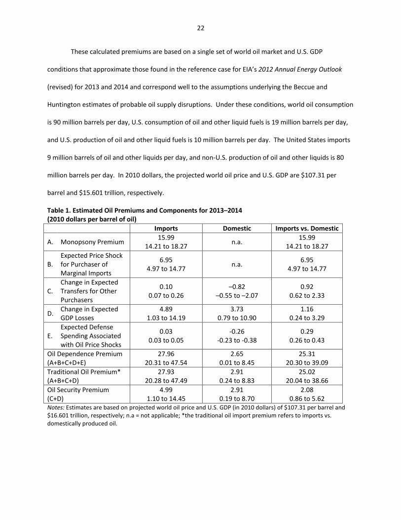
These calculated premiums are based on a single set of world oil market and U.S. GDP 

conditions that approximate those found in the reference case for EIA’s 2012 Annual Energy Outlook 

(revised) for 2013 and 2014 and correspond well to the assumptions underlying the Beccue and 

Huntington estimates of probable oil supply disruptions.  Under these conditions, world oil consumption 

is 90 million barrels per day, U.S. consumption of oil and other liquid fuels is 19 million barrels per day, 

and U.S. production of oil and other liquid fuels is 10 million barrels per day.  The United States imports 

9 million barrels of oil and other liquids per day, and non‐U.S. production of oil and other liquids is 80 

million barrels per day.  In 2010 dollars, the projected world oil price and U.S. GDP are $107.31 per 

barrel and $15.601 trillion, respectively. 

Table 1. Estimated Oil Premiums and Components for 2013–2014 (2010 dollars per barrel of oil)   Imports  Domestic  Imports vs. Domestic 

A.  Monopsony Premium  15.99 14.21 to 18.27  n.a.  15.99 

14.21 to 18.27 

B. Expected Price Shock for Purchaser of Marginal Imports 

6.95 4.97 to 14.77  n.a.  6.95 

4.97 to 14.77 

C. Change in Expected Transfers for Other Purchasers 

0.10 0.07 to 0.26 

–0.82 –0.55 to –2.07 

0.92 0.62 to 2.33 

D.  Change in Expected GDP Losses 

4.89 1.03 to 14.19 

3.73 0.79 to 10.90 

1.16 0.24 to 3.29 

E. Expected Defense Spending Associated with Oil Price Shocks 

0.03 0.03 to 0.05 

‐0.26 ‐0.23 to ‐0.38 

0.29 0.26 to 0.43 

Oil Dependence Premium (A+B+C+D+E) 

27.96 20.31 to 47.54  

2.65 0.01 to 8.45 

25.31 20.30 to 39.09 

Traditional Oil Premium* (A+B+C+D) 

27.93 20.28 to 47.49 

2.91 0.24 to 8.83 

25.02 20.04 to 38.66 

Oil Security Premium (C+D) 

4.99 1.10 to 14.45 

2.91 0.19 to 8.70 

2.08 0.86 to 5.62 

Notes: Estimates are based on projected world oil price and U.S. GDP (in 2010 dollars) of $107.31 per barrel and $16.601 trillion, respectively; n.a = not applicable; *the traditional oil import premium refers to imports vs. domestically produced oil.    

   

23  

3.1.1 Oil Premium Components 

Our framework finds a considerable difference in the various oil premiums for the consumption 

of imported and domestic oil.  Two of these differences are the monopsony premium and the expected 

price shock faced by the purchaser of the marginal barrel of oil.  The purchase of domestic oil does not 

involve the monopsony premium because the transfers would be within the United States.  Similarly, 

purchase of the marginal barrel of oil exposes the purchaser to a price shock—whether the purchase is 

imported or domestic—but the transfers associated with the consumption of domestic oil would be 

strictly within the United States. 

We also find the purchase of imported oil increases the transfers for inframarginal purchases of 

imported oil; whereas the purchase of domestic oil reduces the transfers for the inframarginal 

purchases of imported oil.  An increase in oil imports increases the size of expected price shocks because 

it increases the size of potential disruptions in unstable regions of the world.  Conversely, increasing 

domestic oil production weakens the expected price response because it increases the share of the oil 

market coming from stable supplies.  These pricing effects are also at work in the differential estimates 

for expected GDP losses and expected defense spending. 

3.1.2 Oil Dependence Premiums 

As shown in Table 1, the oil dependence premium for U.S. consumption of imported oil includes 

the monopsony premium, the expected price shock for the purchaser of marginal imports, the change in 

expected transfers for inframarginal purchases, the change in expected GDP losses, and the change in 

expected defense spending associated with oil price shocks.  The oil dependence premium for 

consumption of domestically produced oil excludes the first two above components but includes the 

remaining three components: the change in expected transfers for inframarginal purchases, the change 

in expected GDP losses, and the change in expected defense spending associated with oil price shocks.  

24  

The difference between the estimates, which is the cost of substituting a barrel of imported oil for a 

barrel of domestically produced oil, is $25.31 per barrel in a range of $20.30 to $39.09. 

3.1.3 Traditional Oil Premiums 

The traditional oil premiums, such as those developed by Landberg et al. (1979), Bohi and 

Montgomery (1982a, 1982b), and Leiby (2007), exclude the change in expected defense spending 

associated with oil price shocks and emphasize the difference between reliance on imported and 

domestic oil.  Taking the difference between the traditional estimates associated with U.S. consumption 

of imported oil and domestically produced oil yields $25.02 per barrel in a range of $20.04 to $38.66. 

Thus, this measure is virtually the same as the broader estimate including military expenditures. 

3.1.4 Oil Security Premiums 

As discussed above, Brown and Huntington (2013) identify the oil security premium as including 

only the change in expected transfers for inframarginal purchases and expected GDP losses.  Using just 

these two elements, we find an oil security premium for U.S. consumption of imported oil of $4.99 per 

barrel in a range of $1.10 to $14.45.  The estimated range for U.S. consumption of domestically 

produced oil is $2.91 per barrel in a range of $0.19 to $8.70.  The difference between reliance on 

imported and domestic oil is $2.08 per barrel in a range of $0.86 to $5.62. 

3.2 Reference Case (AEO 2012) 

  We use EIA’s 2012 Annual Energy Outlook as the basis for calculating oil dependence and oil 

security premiums from 2010 to 2035.  In the reference case, world oil consumption is projected to 

grow from 87.05 million barrels per day in 2010 to 109.50 million barrels per day in 2035. U.S. oil 

consumption is predicted to grow from 19.17 million barrels per day to 19.90 million barrels per day.  To 

meet this added demand, non‐U.S. production is projected to grow from 77.36 million barrels per day to 

96.76 million barrels per day.  U.S. production is projected to grow at a faster rate, from 9.69 million 

barrels per day in 2010 to 12.74 million barrels per day in 2035, including non‐petroleum liquids.  As a 

25  

result, projected U.S. oil imports decline from 9.48 million barrels per day in 2010 to 7.15 million barrels 

per day in 2035.  During the same period, world oil prices are projected to rise from $79.39 per barrel to 

$144.98 per barrel.  U.S. GDP is projected at $14,970 billion for 2012 and grows to $27,238 billion in 

2035.  All values are in 2010 dollars. 

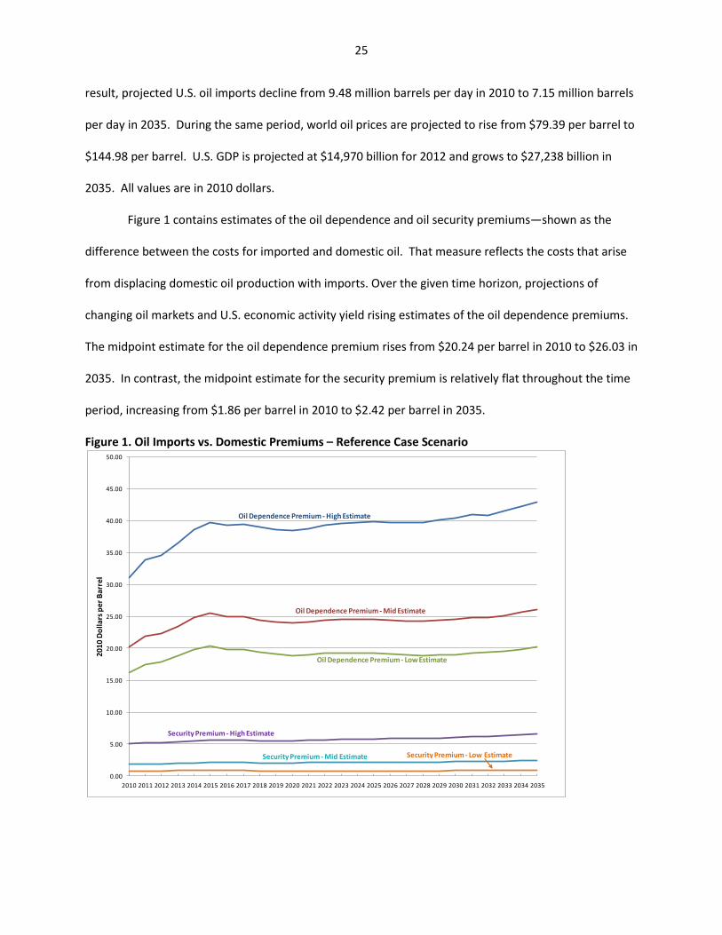
Figure 1 contains estimates of the oil dependence and oil security premiums—shown as the 

difference between the costs for imported and domestic oil.  That measure reflects the costs that arise 

from displacing domestic oil production with imports. Over the given time horizon, projections of 

changing oil markets and U.S. economic activity yield rising estimates of the oil dependence premiums.  

The midpoint estimate for the oil dependence premium rises from $20.24 per barrel in 2010 to $26.03 in 

2035.  In contrast, the midpoint estimate for the security premium is relatively flat throughout the time 

period, increasing from $1.86 per barrel in 2010 to $2.42 per barrel in 2035. 

Figure 1. Oil Imports vs. Domestic Premiums – Reference Case Scenario 

 0.00

5.00

10.00

15.00

20.00

25.00

30.00

35.00

40.00

45.00

50.00

2010 2011 2012 2013 2014 2015 2016 2017 2018 2019 2020 2021 2022 2023 2024 2025 2026 2027 2028 2029 2030 2031 2032 2033 2034 2035

2010 Dollars per Barrel

Oil Dependence Premium ‐ High Estimate

Oil Dependence Premium ‐Mid Estimate

Oil Dependence Premium ‐ Low Estimate

Security Premium ‐ High Estimate

Security Premium ‐Mid Estimate Security Premium ‐ Low Estimate

26  

  Gains in the oil dependence premium arise largely from growth in oil prices and U.S. GDP.  The 

monopsony premium, expected price shock for the marginal purchase of imports, and change in 

expected GDP losses grow significantly over this time.  The monopsony premium increases by $0.96 per 

barrel over the time period, while the expected price shock and losses in GDP increase by $4.17 and 

$3.57 per barrel, respectively. 

  The range of estimates about either midpoint is considerable.  The low estimate of the oil 

dependence premium rises from $16.18 per barrel in 2010 to $20.23 per barrel in 2035, while the high 

estimate grows from $31.18 in 2010 to $42.92 in 2035.  Similarly, estimates of the security externality 

premium range from $0.74 to $5.05 per barrel in 2010 and grow to $0.87 to $6.61 per barrel in 2035. 

3.3 High Economic Growth (AEO 2012) 

  In addition to the reference case, the EIA provides other scenarios in its projections from 2010 

to 2035.  In this section, we consider the implications of a scenario in which the EIA projected stronger 

world economic growth.  In particular, the high economic growth scenario shows U.S. GDP rising to 

$30,063 billion (2010 dollars) in 2035, instead of the $27,238 billion projected in the reference case.   

The additional economic growth leads to stronger growth in world oil consumption, which is projected 

at 110.77 million barrels per day in 2035, instead of the 109.50 projected in the reference case.  U.S. oil 

consumption is also projected to grow more strongly, from 19.17 million barrels per day in 2010 to 

21.17 million barrels per day in 2035.  In the reference case, projected U.S. oil consumption is 19.90 

million barrels per day in 2035.  

Most of the additional oil consumption is met by production from non‐U.S. sources, which are 

projected to provide 97.75 million barrels per day in 2035.  U.S. production is predicted to rise only by 

0.16 million barrels per day above the reference case.  The small gains in U.S. production combined with 

the additional growth in consumption boost U.S. imports by 0.66 million barrels per day in 2035 over the 

reference case. 

27  

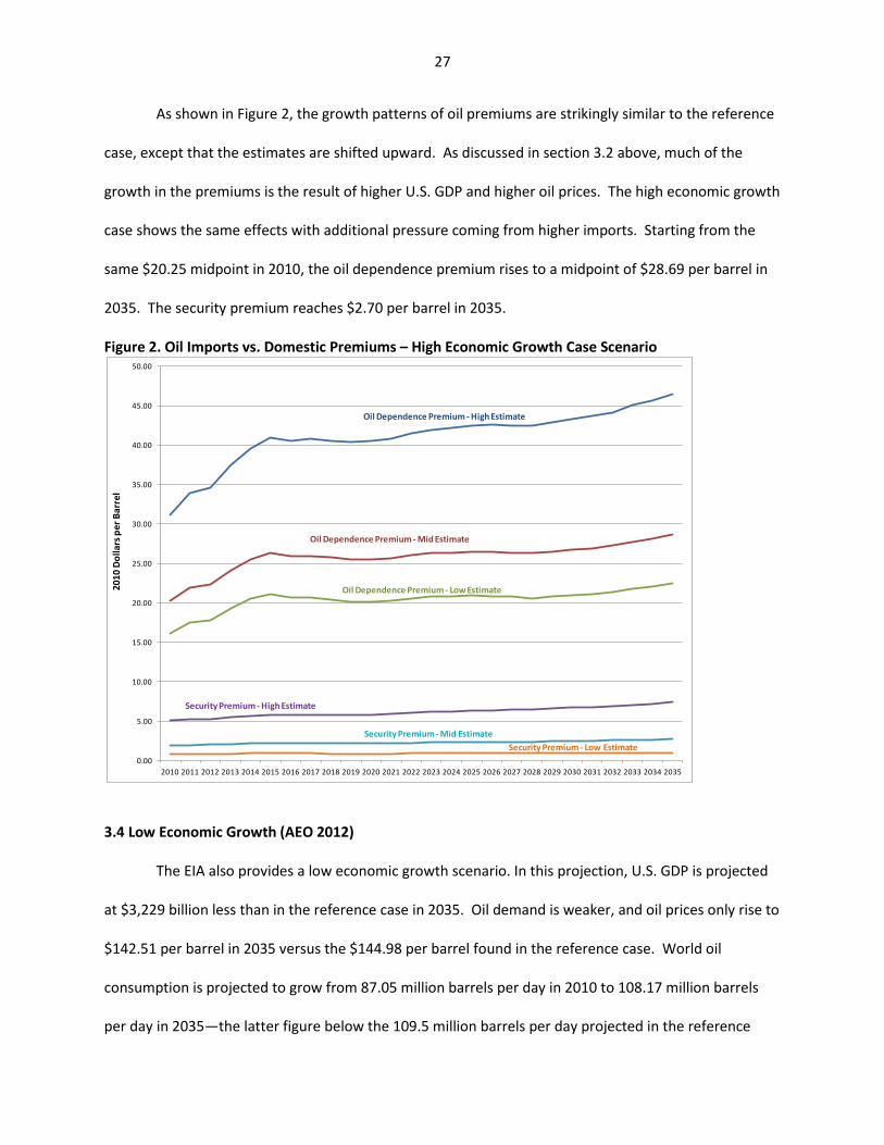
As shown in Figure 2, the growth patterns of oil premiums are strikingly similar to the reference 

case, except that the estimates are shifted upward.  As discussed in section 3.2 above, much of the 

growth in the premiums is the result of higher U.S. GDP and higher oil prices.  The high economic growth 

case shows the same effects with additional pressure coming from higher imports.  Starting from the 

same $20.25 midpoint in 2010, the oil dependence premium rises to a midpoint of $28.69 per barrel in 

2035.  The security premium reaches $2.70 per barrel in 2035. 

Figure 2. Oil Imports vs. Domestic Premiums – High Economic Growth Case Scenario 

 

 3.4 Low Economic Growth (AEO 2012) 

  The EIA also provides a low economic growth scenario. In this projection, U.S. GDP is projected 

at $3,229 billion less than in the reference case in 2035.  Oil demand is weaker, and oil prices only rise to 

$142.51 per barrel in 2035 versus the $144.98 per barrel found in the reference case.  World oil 

consumption is projected to grow from 87.05 million barrels per day in 2010 to 108.17 million barrels 

per day in 2035—the latter figure below the 109.5 million barrels per day projected in the reference 

0.00

5.00

10.00

15.00

20.00

25.00

30.00

35.00

40.00

45.00

50.00

2010 2011 2012 2013 2014 2015 2016 2017 2018 2019 2020 2021 2022 2023 2024 2025 2026 2027 2028 2029 2030 2031 2032 2033 2034 2035

2010 Dollars per Barrel

Oil Dependence Premium ‐ High Estimate

Oil Dependence Premium ‐Mid Estimate

Oil Dependence Premium ‐ LowEstimate

SecurityPremium ‐ High Estimate

Security Premium ‐Mid EstimateSecurity Premium ‐ Low Estimate

28  

case.  The outlook also shows U.S. oil consumption decreasing from 19.17 million barrels per day in 2010 

to 18.57 million barrels per day in 2035.  U.S. oil production is projected to grow at a slower rate than in 

the reference case.  U.S. imports decline from 9.48 million barrels per day in 2010 to 6.23 million barrels 

per day in 2035. 

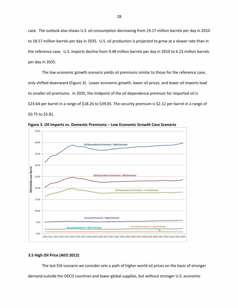
The low economic growth scenario yields oil premiums similar to those for the reference case, 

only shifted downward (Figure 3).  Lower economic growth, lower oil prices, and lower oil imports lead 

to smaller oil premiums.  In 2035, the midpoint of the oil dependence premium for imported oil is 

$23.64 per barrel in a range of $18.26 to $39.65. The security premium is $2.12 per barrel in a range of 

$0.75 to $5.81. 

Figure 3. Oil Imports vs. Domestic Premiums – Low Economic Growth Case Scenario 

 

 3.5 High Oil Price (AEO 2012) 

  The last EIA scenario we consider sets a path of higher world oil prices on the basis of stronger 

demand outside the OECD countries and lower global supplies, but without stronger U.S. economic 

0.00

5.00

10.00

15.00

20.00

25.00

30.00

35.00

40.00

45.00

2010 2011 2012 2013 2014 2015 2016 2017 2018 2019 2020 2021 2022 2023 2024 2025 2026 2027 2028 2029 2030 2031 2032 2033 2034 2035

2010 Dollars per Barrel

Oil Dependence Premium ‐Mid Estimate

Oil Dependence Premium ‐ Low Estimate

Security Premium ‐ High Estimate

Security Premium ‐Mid Estimate Security Premium ‐ Low Estimate

Oil Dependence Premium ‐ High Estimate

29  

growth.  World oil consumption is projected at 122.9 million barrels per day in 2035, which boosts the 

price to $200.36 per barrel.  The high prices result in reduced U.S. oil consumption, with consumption 

slipping from 19.17 million barrels per day in 2010 to 19.12 million barrels per day in 2035.  Higher oil 

prices also stimulate U.S. production, which leads to a projection for 2035 that is 0.57 million barrels per 

day higher than in the reference case.  As the result of reduced U.S. oil consumption and increased U.S. 

oil production, U.S. oil imports slide to a projected 4.02 million barrels per day in 2035. 

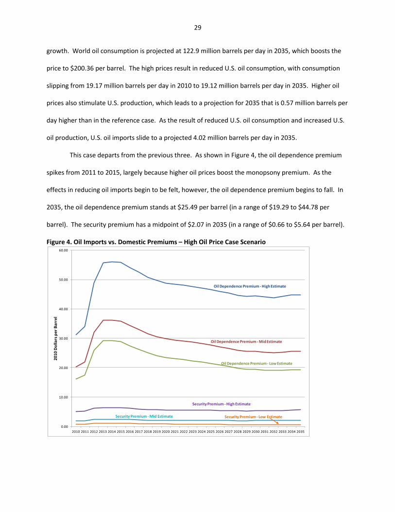
This case departs from the previous three.  As shown in Figure 4, the oil dependence premium 

spikes from 2011 to 2015, largely because higher oil prices boost the monopsony premium.  As the 

effects in reducing oil imports begin to be felt, however, the oil dependence premium begins to fall.  In 

2035, the oil dependence premium stands at $25.49 per barrel (in a range of $19.29 to $44.78 per 

barrel).  The security premium has a midpoint of $2.07 in 2035 (in a range of $0.66 to $5.64 per barrel). 

Figure 4. Oil Imports vs. Domestic Premiums – High Oil Price Case Scenario 

 

    

0.00

10.00

20.00

30.00

40.00

50.00

60.00

2010 2011 2012 2013 2014 2015 2016 2017 2018 2019 2020 2021 2022 2023 2024 2025 2026 2027 2028 2029 2030 2031 2032 2033 2034 2035

2010 Dollars per Barrel

Oil Dependence Premium ‐ High Estimate

Oil Dependence Premium ‐MidEstimate

Oil Dependence Premium ‐ Low Estimate

Security Premium ‐ High Estimate

SecurityPremium ‐ Low EstimateSecurity Premium ‐Mid Estimate

30  

3.6. Changes in World Oil Markets and U.S. Import Dependence 

In addition to examining four scenarios presented by the EIA, we develop our own scenario to 

account for the differences between the 2009 and 2012 Annual Energy Outlooks. In the three years 

between these two outlooks, the known quantities of oil resources in the United States increased.  If we 

create a new scenario—derived from the EIA’s 2012 reference case scenario—in which these additional 

resources do not exist, we can examine how the growth of U.S. oil resources has affected the costs of 

U.S. oil dependence. 

To develop the scenario, we use the Static Energy Analysis Model (SEAM) to assess how more 

conservative assumptions about the U.S. resource base would affect world oil market conditions.8  

SEAM was developed to project how changes in energy market conditions or policy will affect U.S. 

energy markets—including oil, natural gas, coal, and electricity prices; oil, natural gas, coal, and 

electricity consumption; the production of oil, natural gas, and coal; and the transformation of fossil 

energy, nuclear power, and renewable energy sources into electricity.  The model’s oil sector is 

integrated into a world oil market.  Natural gas, coal, and electricity have international links through 

imports and exports.   

For the present exercise, we calibrated SEAM to use the EIA’s 2012 reference case scenario as its 

base case.  We then reduce U.S. conventional and biofuel oil resources to develop projections for world 

oil prices and consumption, U.S. natural gas markets, U.S. coal markets, and U.S. electricity markets.  We 

find that reducing the oil resources available to the model puts the world oil market on a higher price 

trajectory, much like that reported in section 3.5.   

With the reductions in oil supply phased in over a 10‐year period from 2010 to 2020, the 

projected price of oil is higher than in the reference case in each year beginning in 2012.  In that year, 

we find oil prices are $0.54 per barrel higher than in the reference case.  By 2015, the price difference is 

                                                           8 SEAM is documented in Allaire and Brown (2012) and Brown, Kennelly, and Maravich (2012). 

31  

$1.62 per barrel.  From 2016‐2035, the difference in price is over $2.00 per barrel with the highest 

differential being $2.89 per barrel in 2028.    

In comparison to the EIA’s reference case, the forecast for conventional U.S. oil supply shows 

decreased production in all years, with reductions of more than 1 million barrels per day from 2016 

through 2022.  In 2020, oil production is projected at 1.76 million barrels per day less.  After 2022, the 

difference with the reference case narrows and is less than 0.5 million barrels from 2025‐2035.  

Nonetheless, the higher projected trajectory for oil prices weakens the effect of reduced resources on 

conventional U.S. oil production.  

Higher oil prices stimulate U.S. production of biofuels, which actually show slight increases over 

the reference case from 2010 through 2023.  After 2023, the counterfactual shows U.S. production 

biofuels is lower than in the reference case.  Higher oil prices also reduce total U.S. consumption of oil 

and other liquids below the reference case for 2013 through 2035. Consumption is 0.01 million barrels 

per day lower in 2013 and more than 0.1 million barrels per day lower from 2016 through 2035. 

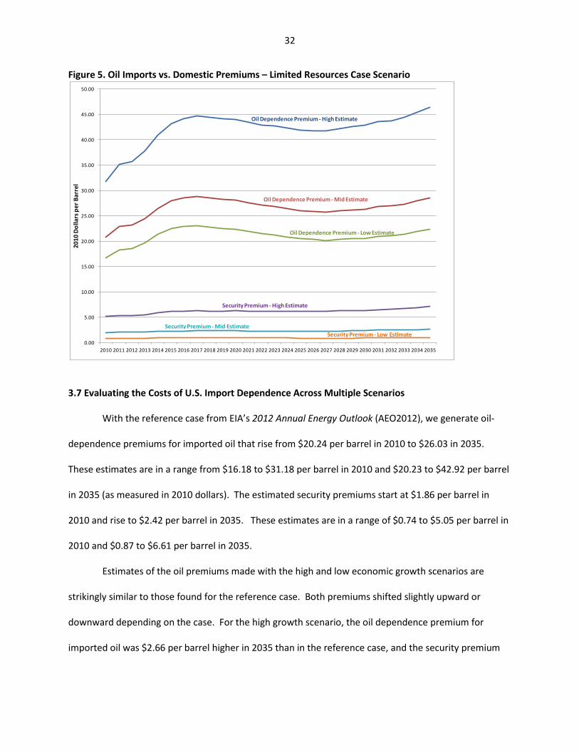
The changes in U.S. oil production and consumption increase U.S. reliance on oil imports from 

2010 to 2035—with the largest estimates concentrated in the period from 2015 to 2023.  As shown in 

Figure 5, reduced domestic oil resources mean higher oil dependence premiums than for the reference 

case.  The midpoint estimate for 2010 is $0.49 per barrel higher.  For 2017, the midpoint estimate is 

$3.80 per barrel higher.  At 2035, the midpoint estimate is $2.45 per barrel higher.  In general, the 

estimates run about 10‐15 percent higher.  We also find slightly higher estimates for the oil security 

premiums, but by a smaller percentage. 

 

   

32  

Figure 5. Oil Imports vs. Domestic Premiums – Limited Resources Case Scenario 

   3.7 Evaluating the Costs of U.S. Import Dependence Across Multiple Scenarios 

With the reference case from EIA’s 2012 Annual Energy Outlook (AEO2012), we generate oil‐

dependence premiums for imported oil that rise from $20.24 per barrel in 2010 to $26.03 in 2035.  

These estimates are in a range from $16.18 to $31.18 per barrel in 2010 and $20.23 to $42.92 per barrel 

in 2035 (as measured in 2010 dollars).  The estimated security premiums start at $1.86 per barrel in 

2010 and rise to $2.42 per barrel in 2035.   These estimates are in a range of $0.74 to $5.05 per barrel in 

2010 and $0.87 to $6.61 per barrel in 2035. 

Estimates of the oil premiums made with the high and low economic growth scenarios are 

strikingly similar to those found for the reference case.  Both premiums shifted slightly upward or 

downward depending on the case.  For the high growth scenario, the oil dependence premium for 

imported oil was $2.66 per barrel higher in 2035 than in the reference case, and the security premium 

0.00

5.00

10.00

15.00

20.00

25.00

30.00

35.00

40.00

45.00

50.00

2010 2011 2012 2013 2014 2015 2016 2017 2018 2019 2020 2021 2022 2023 2024 2025 2026 2027 2028 2029 2030 2031 2032 2033 2034 2035

2010 Dollars per Barrel

Oil Dependence Premium ‐ High Estimate

Oil Dependence Premium ‐Mid Estimate

Oil Dependence Premium ‐ Low Estimate

Security Premium ‐ High Estimate

Security Premium ‐Mid EstimateSecurity Premium ‐ Low Estimate

33  

was $0.28 per barrel higher.  The low growth scenario yielded respective estimates of $2.39 and $0.30 

per barrel lower than the reference case.  

For the scenario with a high oil price trajectory, we find higher initial oil premiums and lower oil 

premiums toward the end of the analysis.  Although the premiums are pushed upward by oil prices, they 

are also reduced as U.S. consumption and imports are reduced.  In 2035, the oil dependence premium 

for imported oil is $0.54 per barrel below the estimate for the reference case, and the estimated 

security premium is $0.35 per barrel lower.  

For the fifth scenario, with reduced U.S. oil resources, we find reduced U.S. oil production, 

higher oil prices, reduced U.S. oil consumption, and higher U.S. oil imports.  Compared to the reference 

case, the increase in oil prices and U.S. oil imports translates into gains of about 10 to 15 percent for the 

oil‐dependence premiums and about 5 to 10 percent for the security premiums.  Differences are 

substantially diminished from 2025 to 2035 as projected imports converge under this scenario and the 

reference case. 

Examining oil dependence and security premiums across all five scenarios, we find increased 

dependence on oil imports and higher world oil prices generate higher estimates of the costs associated 

with dependence on imported oil.  Nonetheless, we find cost estimates that are remarkably similar for 

2035.  In comparison to the reference case, the largest percentage difference for the oil dependence 

premium for imported oil is around 10 percent—for the high economic growth case. The similarity of 

the scenarios largely results from all the scenarios showing the United States becoming substantially less 

dependent on oil imports in the long run—whether that reduction is driven by greater domestic 

resources or by price‐induced conservation and domestic production. 

4. Some Policy Implications 

Ultimately, the purpose of estimating the costs of U.S. dependence on foreign oil is to provide 

guidance for U.S. energy policy. The various approaches that we take for estimating these costs are 

34  

philosophically different and lead to substantially different estimates of the costs of U.S. dependence on 

foreign oil.  As a guide to policy, these differing estimates are consistent with relatively little intervention 

or considerably more intervention.    

The narrower oil‐security approach, developed by Brown and Huntington (2013), finds relatively 

small costs associated with U.S. dependence on imported oil rather than domestically produced oil.  

Concentrating on what they consider security externalities, Brown and Huntington include the change in 

expected transfers and the expected GDP losses associated with the marginal barrel of oil consumption.  

For the scenarios we examine, the estimated security premiums for displacing domestic oil with 

imported oil are relatively small—about 2‐3 percent of projected world oil prices.  The estimates start at 

$1.86 per barrel in 2010 and rise to $2.42 per barrel in 2035.  These estimates are in a range of $0.74 to 

$5.05 per barrel in 2010 and $0.87 to $6.61 per barrel in 2035.  With these small estimates, a relatively 

modest intervention in the oil market to displace oil imports with domestic oil production is suggested. 

The broader approach used throughout the literature on U.S. oil import dependence, doesn’t 

really distinguish between externalities and other costs.  In addition to the two components used by 

Brown and Huntington, the broader literature includes the exercise of monopsony power, the expected 

price shock faced by the purchaser of marginal imports.  We broadened it slightly (in a quantitative 

sense) by including the expected increase in defense spending associated with oil price shocks.   

With the scenarios we examine, the broader measure results in much higher estimates for the 

costs of U.S. dependence on imported oil—in the range of 20 to 30 percent of world prices.  For the 

reference case in the EIA’s 2012 Annual Energy Outlook, we generate oil dependence premiums for 

imported oil that rise from $20.24 per barrel in 2010 to $26.03 in 2035.  These estimates are in a range 

from $16.18 to $31.18 per barrel in 2010 and $20.23 to $42.92 per barrel in 2035 (as measured in 2010 

dollars).  With these estimates, considerably more intervention in the oil market is suggested. 

35  

We also examined four other scenarios for world oil market conditions—including the high 

growth, low growth, and high oil price scenarios in the 2012 Annual Energy Outlook and scenario of our 

own development that represented lower U.S. oil resources.  As might be expected, higher import 

dependence and higher world oil prices generate larger premiums.  Nonetheless, we found substantially 

similar estimates for the oil premiums across all five of the scenarios we considered.9  That stability 

suggests that the conduct of U.S. oil import policy will remain relatively unaffected by foreseen 

developments in world oil markets.  Substantially different world oil market conditions would yield 

different results. 

4.1 Costs of Oil Dependence 

We also used the analysis to examine the implementation of policy to reduce the expected costs 

of dependence on imported oil below 1 percent of GDP, a target suggested by Greene (2011).  Taking 

the expected costs of imported oil as the oil dependence premium for imports vs. domestically 

produced oil times the quantity of imported oil, we found only the high estimates for the high oil price 

scenario yielded any results that exceeded Greene’s threshold—and that was only for 2012 and 2013 

and by very little. 

Taking a somewhat different approach, we examined the expected costs of U.S. dependence on 

oil.  Taking expected costs to be the oil dependence premium for imported oil times the quantity of 

imported oil plus the oil dependence premium for domestic oil times the quantity of domestic oil, we 

found the high estimates for all five scenarios yielded an expected cost that slightly exceeded 1 percent 

of GDP for 2010 through 2017 or 2018, depending on the scenario.  The low and mean estimates for all 

scenarios yielded results that were well below the 1 percent threshold for all years. 

                                                           9 In comparison to the reference case, the largest percentage difference for the oil dependence premium is around 10 percent in 2035—for the high economic growth case.  The convergence of the scenarios is largely the result of all the scenarios showing the United States becoming substantially less dependent on oil imports in the long run.  In some cases, greater domestic resources drive reduced U.S. dependence on oil imports.  In others, price‐induced conservation and domestic oil production lessen the dependence on oil imports. 

36  

5. Some Options for Implementing Policy 

The premium estimates show the value of reducing oil consumption of either domestic or 

imported oil.  These premiums can be applied to many types of policies—taxes, efficiency standards, 

demand‐side policies, or other constraints on market behavior.  The standard would be to adopt policies 

that cost no more than the estimated premium amounts.   

If retaliatory actions by foreign oil producers can be ruled out, frequently economists will 

recommend taking the direct approach of imposing the appropriate costs—either narrowly or broadly 

measured—as oil import taxes or some other market instrument.10  For instance, the use of the oil 

dependence premium recommends oil import taxes of $20.24 per barrel in 2010 (with a range of $16.18 

to $31.18) for the reference case scenario.  The tax would rise to $26.03 per barrel in 2035 (with a range 

of $20.23 to $42.92).  Much lower import taxes would result from use of the narrower oil security 

premium. 

Economists recognize that import quotas can be set so they are equivalent to import taxes.  We 

estimate that setting oil import quotas to reduce U.S. oil imports by 2.25 million barrels per day (in a 

range of 2.05 million to 2.89 million barrels per day) would be equivalent to imposing the oil 

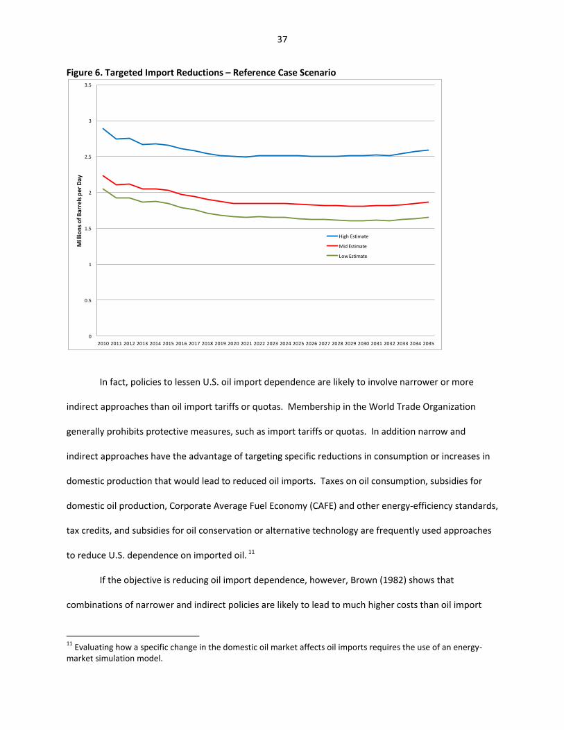
dependence premiums for imported oil for the reference case scenario in 2010 (Figure 6).  With U.S. 

reliance on imports projected to fall, we find the corresponding target for reducing oil imports also falls, 

reaching a low in 2030 of 1.81 million barrels per day (in a range of 1.61 million to 2.51 million barrels 

per day).  After 2030, the targeted reduction in imports rises with the expected level of oil imports, 

reaching 1.87 million barrels per day (in a range of 1.66 million to 2.59 million barrels per day). 

                                                           10 When used to address identified market problems related to oil imports, an oil import tax is not considered a distortionary tax.  Rather, it is a tax to overcome a market distortion.  See Schultze (1977). 

37  

Figure 6. Targeted Import Reductions – Reference Case Scenario

   In fact, policies to lessen U.S. oil import dependence are likely to involve narrower or more 

indirect approaches than oil import tariffs or quotas.  Membership in the World Trade Organization 

generally prohibits protective measures, such as import tariffs or quotas.  In addition narrow and 

indirect approaches have the advantage of targeting specific reductions in consumption or increases in 

domestic production that would lead to reduced oil imports.  Taxes on oil consumption, subsidies for 

domestic oil production, Corporate Average Fuel Economy (CAFE) and other energy‐efficiency standards, 

tax credits, and subsidies for oil conservation or alternative technology are frequently used approaches 

to reduce U.S. dependence on imported oil. 11 

If the objective is reducing oil import dependence, however, Brown (1982) shows that 

combinations of narrower and indirect policies are likely to lead to much higher costs than oil import 

                                                           11 Evaluating how a specific change in the domestic oil market affects oil imports requires the use of an energy‐market simulation model. 

0

0.5

1

1.5

2

2.5

3

3.5

2010 2011 2012 2013 2014 2015 2016 2017 2018 2019 2020 2021 2022 2023 2024 2025 2026 2027 2028 2029 2030 2031 2032 2033 2034 2035

Millions of B

arrels pe

r Day

High Estimate

Mid Estimate

Low Estimate

38  

taxes.12  As they have been adopted in the past, combinations of targeted and indirect policies typically 

bring forth fewer measures for reducing oil imports—most often conservation.  In addition, the marginal 

costs of such policies are rarely equated.   

The implications of Brown’s analysis are twofold.  The higher costs of implementing policy ought 

to lead to more conservative reductions in oil imports.  In addition, the calculated oil dependence 

premiums (or oil security premiums) provide a more reasonable guide about how far to pursue any 

given policy than quantity targets. 

Brown’s analysis relies on the idea that prices provide strong, reliable incentives that matter in 

markets.  Other policy analysts, such as McKinsey and Company (2009), take the approach that prices 

are a less effective way to implement policy than other measures.  As they see it, consumers are 

relatively insensitive to price signals.  Ultimately, policy makers must determine whether pricing the 

costs of imported oil or other forms of market intervention are more effective. 

6. Summary and Conclusions 

A considerable body of previous work addresses the non‐environmental costs of U.S. oil 

dependence—taking the approach that these costs exceed the market price paid for the oil.  The 

literature is wide ranging.  It includes arguments from a number of different perspectives within 

economics and at least a few from outside economics.  Most of the literature distinguishes between the 

costs associated with dependence on imported oil and domestically produced oil, but only quantifies the 

differential in costs between the consumption of imported and domestically produced oil. 

In sorting through this wide‐ranging literature, we take the perspective of economists who seek 

to quantify any non‐environmental costs of U.S. dependence on oil that are in excess of the market price 

paid for oil.  In doing so, we calculate three different types of oil premiums.   

                                                           12 Adding environmental costs to the picture does not change the analysis. 

39  

The first type is the relatively narrow oil security premiums developed by Brown and Huntington 

(2013) to address the security externalities associated with dependence on imported and domestic oil.  

This premium quantifies the GDP losses and some of transfers associated with expected oil supply 

shocks, yielding higher estimates costs for the consumption of imported oil than domestically produced 

oil.  For the scenarios we examine, the estimated security premiums for displacing domestic oil with 

imported oil are relatively small—about 2‐3 percent of projected world oil prices.  Abstracting from the 

environmental costs associated with oil production and use, these premiums suggest that only relatively 

modest policies are recommended for reducing U.S. dependence on imported oil in favor of 

domestically produced oil.  A somewhat stronger case can be made for reducing dependence on both 

imported and domestic oil through conservation policies.   

The broader measures we examine take the perspective of identifying all the non‐price, non‐

environmental costs of oil dependence without keeping a sharp focus on externalities.  These measures 

include the traditional oil premium which includes the oil security premium and adds monopsony buying 

power and more of the transfers associated with expected oil supply shocks.  The oil dependence 

premium further includes the increased defense costs associated with expected oil supply shocks, a cost 

we find to be quite small.  These broader measures result in much higher estimates for the costs for 

displacing domestic oil with imported oil—in the range of 20 to 30 percent of world prices.  If we look 

past strict definitions of what constitutes an externality, these premiums suggest that fairly aggressive 

policies are recommended for reducing U.S. dependence on imported oil.  Policies to displace imports 

with conservation or domestic production are nearly equally recommended.

40  

Appendix A: Estimating the Economic Costs of U.S. Oil Dependence 

To estimate the economic costs of U.S. oil dependence, each element of Equations 2 and 3 

needs to be estimated.  Landsberg et al. (1979), as well as numerous others, provide guidance for 

estimating the monopsony premium, :<=:)>𝑄6.  Brown and Huntington (2013) offer guidance for 

estimating the expected costs associated with additional consumption of domestic and imported oil, 

:8;3:)3

 and :8>:)>, respectively.  In addition, we offer a new approach for estimating the defense costs 

associated with oil import dependence. 

A.1 Estimating the Value of Monopsony Buying Power 

  To estimate the monopsony premium associated with oil imports, we simply use the second 

term of Equation 3 above as follows 

                         (A.1)   

where MP is the monoposony premium for imported oil.  The expression can be evaluated using long‐

term elasticities of non‐U.S. supply and demand, market quantities and the world oil price as follows 

                       (A.2) 

where QSROW is non‐U.S. oil production, ηSROW is the price elasticity of non‐U.S. oil supply, QDROW is the 

quantity of non‐U.S. oil consumption, and ηDROW is the price elasticity of non‐U.S. oil demand. 

A.2 Calculating Premiums Associated with Oil Supply Disruptions 

To calculate the premiums associated with oil supply disruptions, we focus on the economic 

losses associated with world oil supply disruptions—the expected GDP losses and wealth transfers.  In 

doing so, we draw directly on Brown and Huntington (2013).  The expected disruption premium for the 

use of imported oil instead of domestically produced oil is the difference between premiums for 

imported and domestic oil. 

MM

w QQPMP

DR OWM

DR OWS R OW

M

S R OW

W

QQ

QQ

PMP

41  

Implementing the Brown and Huntington approach for calculating oil security premiums 

requires an assessment of the probabilities of oil supply disruptions of various sizes, estimated short‐run 

supply and demand elasticities to compute the resulting price shocks, an estimated elasticity of U.S. GDP 

to oil price increases that result from supply disruptions, and a projection of world oil market conditions.  

These parameters and data can be used to calculate how a marginal increase in oil consumption from 

domestic or imported sources affects the expected U.S. GDP losses and transfers that result from each 

possible oil supply disruption.  The probabilities are then used to combine the separate estimates. 

Following Brown and Huntington, the disruption probabilities and sizes are adapted from a 

recent Energy Modeling Forum (EMF) study documented by Beccue and Huntington (2005).  The short‐

run demand and supply elasticities are adapted from the economics literature, as are the elasticities of 

U.S. GDP to oil price shocks.  The 2012 Annual Energy Outlook produced by the Energy Information 

Administration (EIA) is used to project world oil market conditions. 

A.2.1 Analytics of an Oil Premium Associated with a Disruption 

The oil disruption premium associated with the consumption of domestically produced oil 

represents the increased costs of the expected income transfers to foreign oil producers and GDP losses 

that result from changes in the consumption of domestically produced oil.   If we assume the probability 

and size of disruptions are separable, Brown and Huntington show that the security premium term for 

the consumption of domestic oil from Equation 2, :8;3:)3, can be rewritten as a product of individual 

probabilities and disruptions as follows 

                   (A.3)  

where SD is the oil dependence premium for the consumption of domestically produced oil,   and ∆Qi 

n

i D

ii

n

iM

D

iiD Q

QPYQQ

QPS11

))(()(

�

i

42  

are the respective probability and size of each oil supply disruption i, P is the price of oil, QD is U.S. oil 

production, QM is U.S. oil imports, and Y is U.S. GDP.13 

As Equation A.3 shows, two factors shape the security premium when increased consumption is 

met only with domestically produced oil.  As shown by the terms under the first summation, the 

increase in secure production reduces the price increase resulting from any external oil supply shock, 

which reduces the transfers to foreign oil producers when such a shock occurs.  For the terms under the 

second summation, increased consumption of domestically produced oil increases the exposure of 

aggregate economic activity to the price effects of oil supply shocks.  At the same time, a marginal 

increase in secure domestic oil production reduces the relative importance of insecure supplies in the 

global oil market, which reduces the expected price shocks and dampens the expected GDP losses.   

  In a similar manner, the disruption premium for the consumption of imported oil represents the 

increased costs of the expected income transfers to foreign oil producers and GDP losses that result 

from changes in the consumption of imported oil.  Again, if we assume that the probability and size of 

disruptions are separable, Brown and Huntington show that the disruption premium term for the 

consumption of imported oil from Equation 3, :8>:)>, can be rewritten as a product of individual 

probabilities and disruptions.  Departing from Brown and Huntington, we also include a term for the 

expected change in prices associated with consumption of the marginal barrel of oil to obtain the 

following 

                 (A.4) 

where SI is the oil dependence premium for the consumption of imported oil. 

As Equation A.4 shows, three factors affect the oil dependence premium when an increase in 

consumption is met with imported oil.  As shown by the terms under the first summation, the increase 

                                                           13 Note that ∑  when one state represents a zero disruption. 

n

i M

ii

n

iii

n

iM

M

iiI Q

QPYQPQQ

QPS111

))(()()(

�

i 1

43  

of insecure production boosts the price increase resulting from any oil supply shock, which increases the 

transfers to foreign oil producers when such a shock occurs.  As shown by the terms under the second 

summation, the purchaser of the marginal barrel of oil faces a higher expected price when there is an oil 

supply shock.  The terms under the third summation show that an increase in imported oil increases the 

exposure of aggregate economic activity to the price effects of oil supply shocks.  At the same time, a 

marginal increase in U.S. oil imports increases the output of insecure oil supplies, which increases 

expected oil price shocks and exacerbates the expected GDP losses.  

In taking the Brown and Huntington approach, we treat expected world oil supply disruptions as 

discrete probabilistic episodes that are exogenous.  The size of each disruption is a function of world oil 

market conditions and responds to changes in U.S. oil imports. 

A.2.2 Probability of Supply Disruptions 

  Following Brown and Huntington, we adapt the Beccue and Huntington (2005) risk assessment.  

Beccue and Huntington developed a risk assessment framework and evaluated the likelihood of foreign 

oil supply disruptions over a decade‐long period.  Although domestic problems and severe weather 

could result in significant disruptions, the study focused on geopolitical, military, and terrorist causes of 

disruptions abroad.14  Conducted as a structured survey of experts, the final results provide a subjective 

assessment of the size, likelihood, and duration of disruptions over the 10‐year period from 2005 to 

2014.  Disruptions are expressed as net outcomes, after all surplus capacity from market participants 

and foreign governments has been used. 

  We convert their decadal estimates to the annual values shown in Table A.1.  Each decadal 

estimate (denoted as  ) is the probability of at least one or more disruptions over the decade.  If the 

stability over the decade (1– ) has an equal likelihood of happening in each year, the annual 

                                                           14 In using the Beccue–Huntington estimates, we abstract from natural supply disruptions, such as those arising from hurricanes or other severe weather. 

�

d

�

d

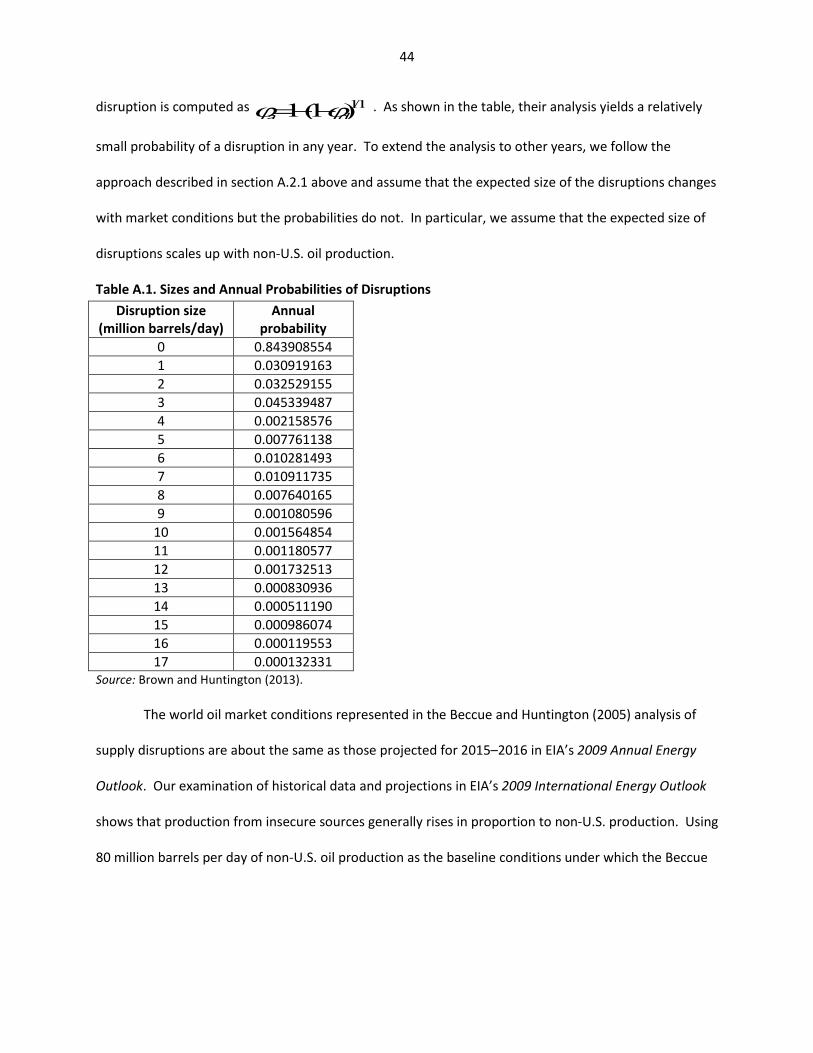
44  

disruption is computed as  .  As shown in the table, their analysis yields a relatively 

small probability of a disruption in any year.  To extend the analysis to other years, we follow the 

approach described in section A.2.1 above and assume that the expected size of the disruptions changes 

with market conditions but the probabilities do not.  In particular, we assume that the expected size of 

disruptions scales up with non‐U.S. oil production. 

Table A.1. Sizes and Annual Probabilities of Disruptions Disruption size 

(million barrels/day) Annual 

probability 0  0.843908554 1  0.030919163 2  0.032529155 3  0.045339487 4  0.002158576 5  0.007761138 6  0.010281493 7  0.010911735 8  0.007640165 9  0.001080596 10  0.001564854 11  0.001180577 12  0.001732513 13  0.000830936 14  0.000511190 15  0.000986074 16  0.000119553 17  0.000132331 

Source: Brown and Huntington (2013).  

The world oil market conditions represented in the Beccue and Huntington (2005) analysis of 

supply disruptions are about the same as those projected for 2015–2016 in EIA’s 2009 Annual Energy 

Outlook.  Our examination of historical data and projections in EIA’s 2009 International Energy Outlook 

shows that production from insecure sources generally rises in proportion to non‐U.S. production.  Using 

80 million barrels per day of non‐U.S. oil production as the baseline conditions under which the Beccue 

1 0/1)1(1 da

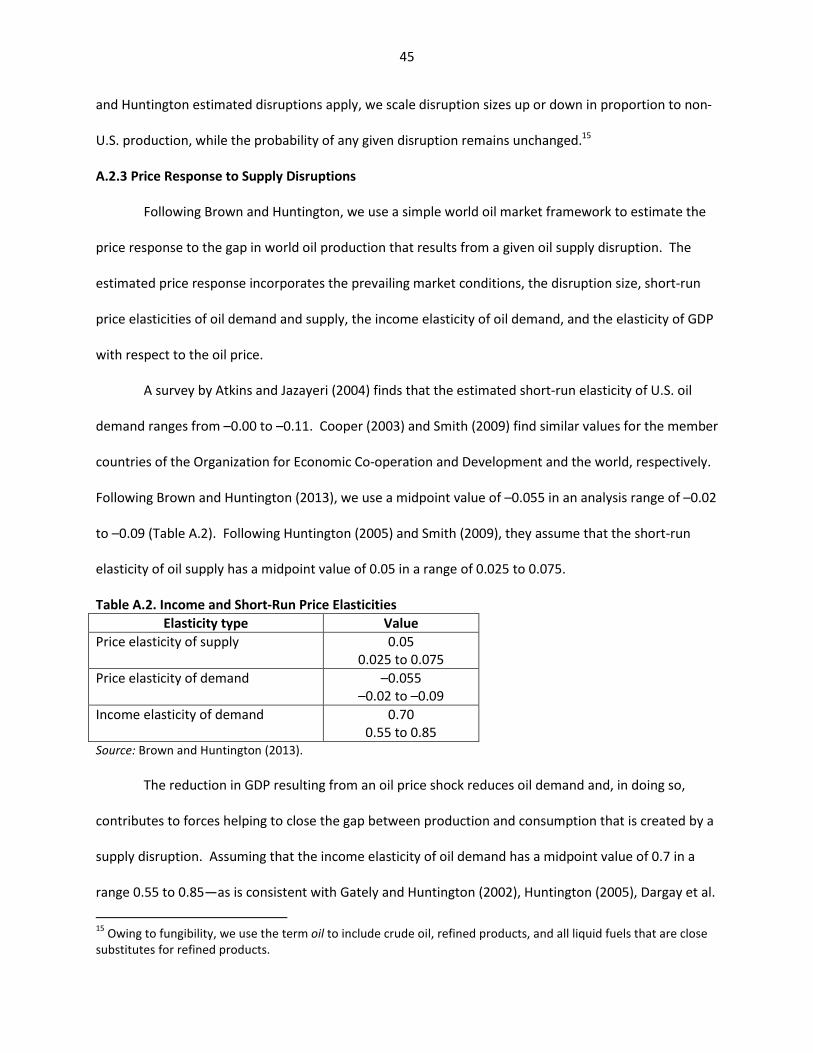
45  

and Huntington estimated disruptions apply, we scale disruption sizes up or down in proportion to non‐

U.S. production, while the probability of any given disruption remains unchanged.15 

A.2.3 Price Response to Supply Disruptions 

Following Brown and Huntington, we use a simple world oil market framework to estimate the 

price response to the gap in world oil production that results from a given oil supply disruption.  The 

estimated price response incorporates the prevailing market conditions, the disruption size, short‐run 

price elasticities of oil demand and supply, the income elasticity of oil demand, and the elasticity of GDP 

with respect to the oil price. 

A survey by Atkins and Jazayeri (2004) finds that the estimated short‐run elasticity of U.S. oil 

demand ranges from –0.00 to –0.11.  Cooper (2003) and Smith (2009) find similar values for the member 

countries of the Organization for Economic Co‐operation and Development and the world, respectively.  

Following Brown and Huntington (2013), we use a midpoint value of –0.055 in an analysis range of –0.02 

to –0.09 (Table A.2).  Following Huntington (2005) and Smith (2009), they assume that the short‐run 

elasticity of oil supply has a midpoint value of 0.05 in a range of 0.025 to 0.075. 

Table A.2. Income and Short‐Run Price Elasticities Elasticity type  Value 

Price elasticity of supply  0.05 0.025 to 0.075  

Price elasticity of demand  –0.055 –0.02 to –0.09 

Income elasticity of demand  0.70 0.55 to 0.85 

Source: Brown and Huntington (2013).  

The reduction in GDP resulting from an oil price shock reduces oil demand and, in doing so, 

contributes to forces helping to close the gap between production and consumption that is created by a 

supply disruption.  Assuming that the income elasticity of oil demand has a midpoint value of 0.7 in a 

range 0.55 to 0.85—as is consistent with Gately and Huntington (2002), Huntington (2005), Dargay et al. 

                                                           15 Owing to fungibility, we use the term oil to include crude oil, refined products, and all liquid fuels that are close substitutes for refined products. 

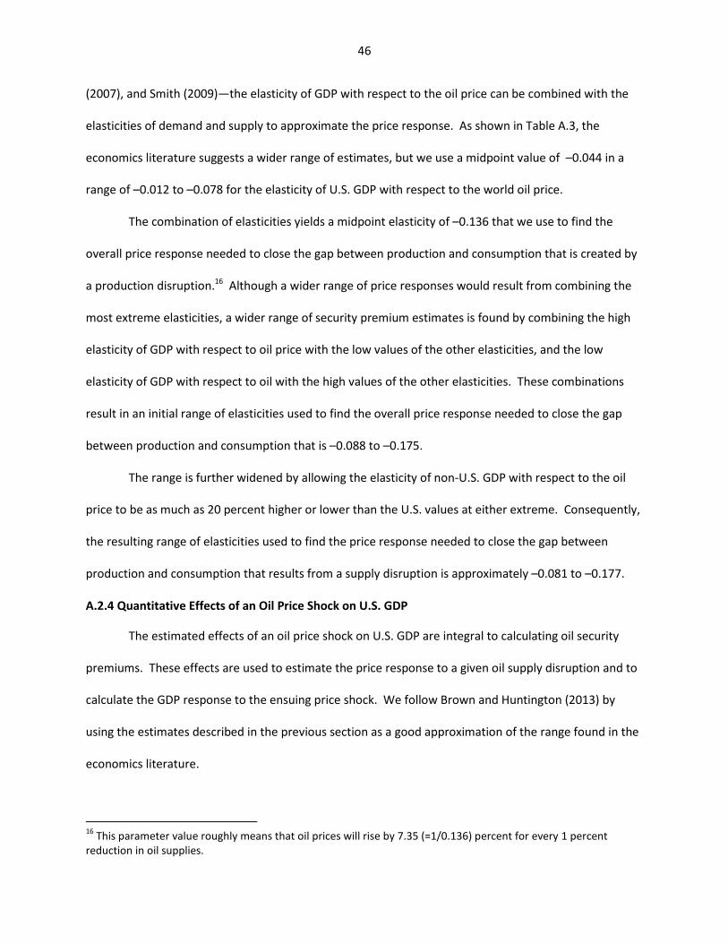
46  

(2007), and Smith (2009)—the elasticity of GDP with respect to the oil price can be combined with the 

elasticities of demand and supply to approximate the price response.  As shown in Table A.3, the 

economics literature suggests a wider range of estimates, but we use a midpoint value of  –0.044 in a 

range of –0.012 to –0.078 for the elasticity of U.S. GDP with respect to the world oil price. 

The combination of elasticities yields a midpoint elasticity of –0.136 that we use to find the 

overall price response needed to close the gap between production and consumption that is created by 

a production disruption.16  Although a wider range of price responses would result from combining the 

most extreme elasticities, a wider range of security premium estimates is found by combining the high 

elasticity of GDP with respect to oil price with the low values of the other elasticities, and the low 

elasticity of GDP with respect to oil with the high values of the other elasticities.  These combinations 

result in an initial range of elasticities used to find the overall price response needed to close the gap 

between production and consumption that is –0.088 to –0.175. 

The range is further widened by allowing the elasticity of non‐U.S. GDP with respect to the oil 

price to be as much as 20 percent higher or lower than the U.S. values at either extreme.  Consequently, 

the resulting range of elasticities used to find the price response needed to close the gap between 

production and consumption that results from a supply disruption is approximately –0.081 to –0.177. 

A.2.4 Quantitative Effects of an Oil Price Shock on U.S. GDP 

The estimated effects of an oil price shock on U.S. GDP are integral to calculating oil security 

premiums.  These effects are used to estimate the price response to a given oil supply disruption and to 

calculate the GDP response to the ensuing price shock.  We follow Brown and Huntington (2013) by 

using the estimates described in the previous section as a good approximation of the range found in the 

economics literature. 

                                                           16 This parameter value roughly means that oil prices will rise by 7.35 (=1/0.136) percent for every 1 percent reduction in oil supplies. 

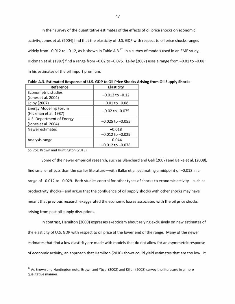
47  

In their survey of the quantitative estimates of the effects of oil price shocks on economic 

activity, Jones et al. (2004) find that the elasticity of U.S. GDP with respect to oil price shocks ranges 

widely from –0.012 to –0.12, as is shown in Table A.3.17  In a survey of models used in an EMF study, 

Hickman et al. (1987) find a range from –0.02 to –0.075.  Leiby (2007) uses a range from –0.01 to –0.08 

in his estimates of the oil import premium. 

Table A.3. Estimated Response of U.S. GDP to Oil Price Shocks Arising from Oil Supply Shocks Reference  Elasticity 

Econometric studies (Jones et al. 2004)  –0.012 to –0.12 

Leiby (2007)  –0.01 to –0.08 Energy Modeling Forum  (Hickman et al. 1987)  –0.02 to –0.075 

U.S. Department of Energy (Jones et al. 2004)  –0.025 to –0.055 

Newer estimates  –0.018 –0.012 to –0.029 

Analysis range  –0.044 –0.012 to –0.078 

Source: Brown and Huntington (2013).  Some of the newer empirical research, such as Blanchard and Gali (2007) and Balke et al. (2008), 

find smaller effects than the earlier literature—with Balke et al. estimating a midpoint of –0.018 in a 

range of –0.012 to –0.029.  Both studies control for other types of shocks to economic activity—such as 

productivity shocks—and argue that the confluence of oil supply shocks with other shocks may have 

meant that previous research exaggerated the economic losses associated with the oil price shocks 

arising from past oil supply disruptions. 

In contrast, Hamilton (2009) expresses skepticism about relying exclusively on new estimates of 

the elasticity of U.S. GDP with respect to oil price at the lower end of the range.  Many of the newer 

estimates that find a low elasticity are made with models that do not allow for an asymmetric response 

of economic activity, an approach that Hamilton (2010) shows could yield estimates that are too low.  It 

                                                           17 As Brown and Huntington note, Brown and Yücel (2002) and Kilian (2008) survey the literature in a more qualitative manner. 

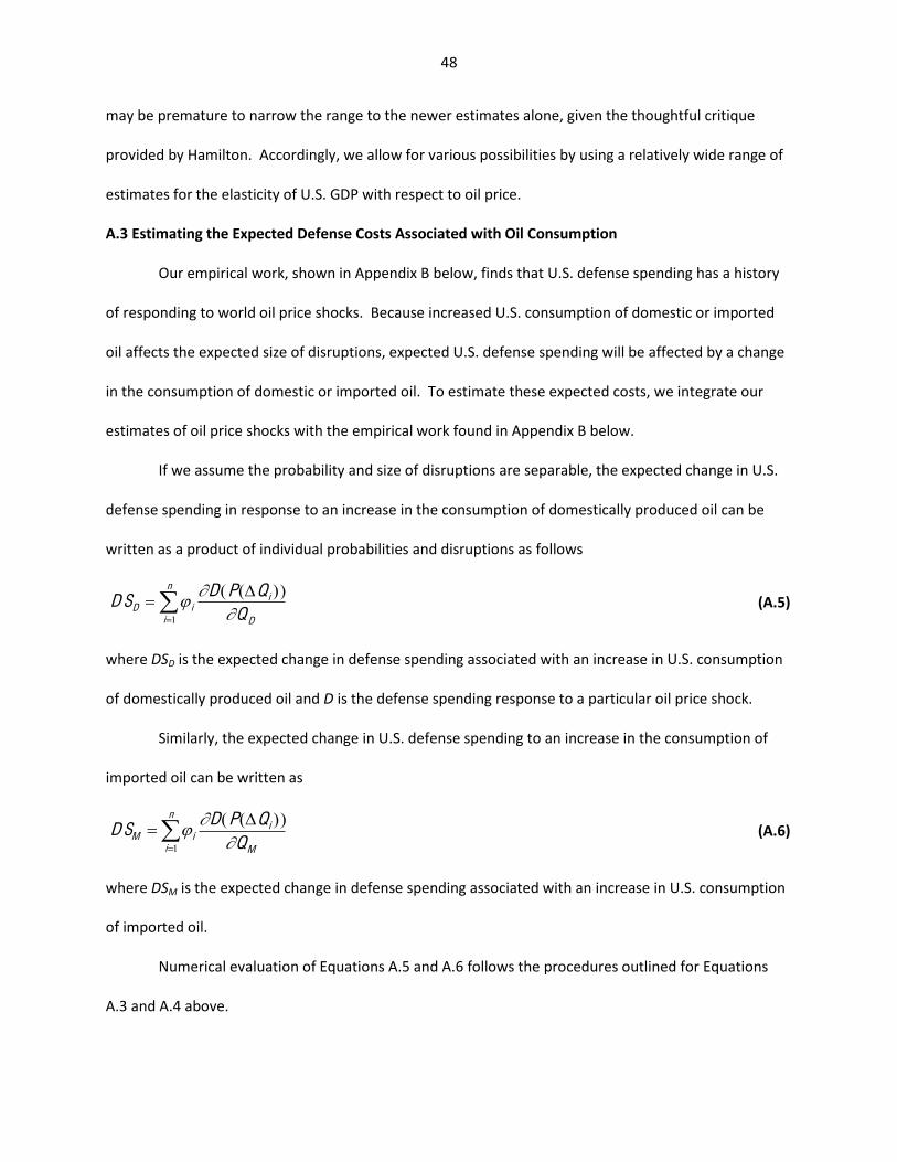
48  

may be premature to narrow the range to the newer estimates alone, given the thoughtful critique 

provided by Hamilton.  Accordingly, we allow for various possibilities by using a relatively wide range of 

estimates for the elasticity of U.S. GDP with respect to oil price. 

A.3 Estimating the Expected Defense Costs Associated with Oil Consumption 

  Our empirical work, shown in Appendix B below, finds that U.S. defense spending has a history 

of responding to world oil price shocks.  Because increased U.S. consumption of domestic or imported 

oil affects the expected size of disruptions, expected U.S. defense spending will be affected by a change 

in the consumption of domestic or imported oil.  To estimate these expected costs, we integrate our 

estimates of oil price shocks with the empirical work found in Appendix B below. 

If we assume the probability and size of disruptions are separable, the expected change in U.S. 

defense spending in response to an increase in the consumption of domestically produced oil can be 

written as a product of individual probabilities and disruptions as follows 

                       (A.5)  

where DSD is the expected change in defense spending associated with an increase in U.S. consumption 

of domestically produced oil and D is the defense spending response to a particular oil price shock. 

Similarly, the expected change in U.S. defense spending to an increase in the consumption of 

imported oil can be written as 

                       (A.6)  

where DSM is the expected change in defense spending associated with an increase in U.S. consumption 

of imported oil. 

  Numerical evaluation of Equations A.5 and A.6 follows the procedures outlined for Equations 

A.3 and A.4 above. 

 

n

i D

iiD Q

QPDD S1

))((

n

i M

iiM Q

QPDD S1

))((

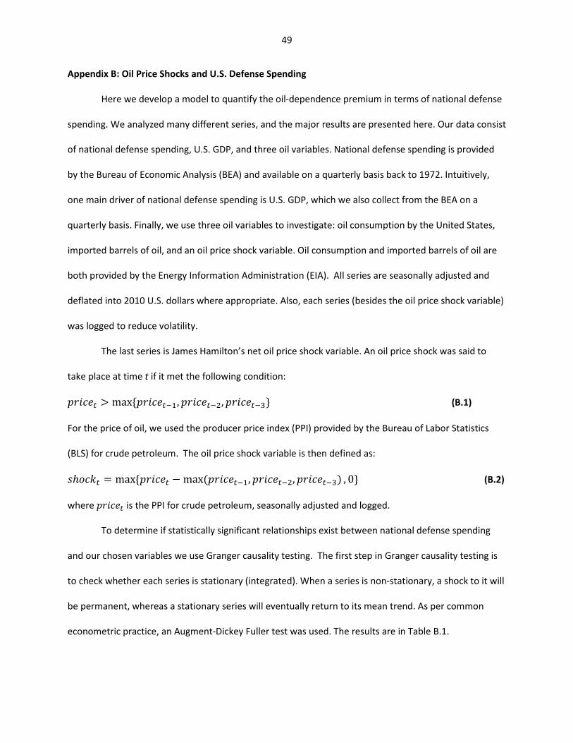
49  

Appendix B: Oil Price Shocks and U.S. Defense Spending  

Here we develop a model to quantify the oil‐dependence premium in terms of national defense 

spending. We analyzed many different series, and the major results are presented here. Our data consist 

of national defense spending, U.S. GDP, and three oil variables. National defense spending is provided 

by the Bureau of Economic Analysis (BEA) and available on a quarterly basis back to 1972. Intuitively, 

one main driver of national defense spending is U.S. GDP, which we also collect from the BEA on a 

quarterly basis. Finally, we use three oil variables to investigate: oil consumption by the United States, 

imported barrels of oil, and an oil price shock variable. Oil consumption and imported barrels of oil are 

both provided by the Energy Information Administration (EIA).  All series are seasonally adjusted and 

deflated into 2010 U.S. dollars where appropriate. Also, each series (besides the oil price shock variable) 

was logged to reduce volatility.  

The last series is James Hamilton’s net oil price shock variable. An oil price shock was said to 

take place at time t if it met the following condition: 

𝑝𝑟𝑖𝑐𝑒D > max {𝑝𝑟𝑖𝑐𝑒DKL, 𝑝𝑟𝑖𝑐𝑒DKN, 𝑝𝑟𝑖𝑐𝑒DKO}               (B.1) 

For the price of oil, we used the producer price index (PPI) provided by the Bureau of Labor Statistics 

(BLS) for crude petroleum.  The oil price shock variable is then defined as: 

𝑠ℎ𝑜𝑐𝑘D = max {𝑝𝑟𝑖𝑐𝑒D − max(𝑝𝑟𝑖𝑐𝑒DKL, 𝑝𝑟𝑖𝑐𝑒DKN, 𝑝𝑟𝑖𝑐𝑒DKO) , 0}             (B.2) 

where 𝑝𝑟𝑖𝑐𝑒D is the PPI for crude petroleum, seasonally adjusted and logged.  

To determine if statistically significant relationships exist between national defense spending 

and our chosen variables we use Granger causality testing.  The first step in Granger causality testing is 

to check whether each series is stationary (integrated). When a series is non‐stationary, a shock to it will 

be permanent, whereas a stationary series will eventually return to its mean trend. As per common 

econometric practice, an Augment‐Dickey Fuller test was used. The results are in Table B.1. 

   

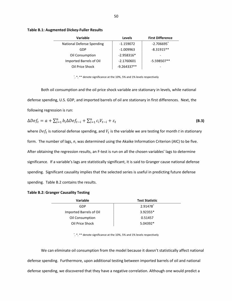
50  

Table B.1: Augmented Dickey‐Fuller Results 

Variable  Levels  First Difference National Defense Spending  ‐1.159072  ‐2.706695+ 

GDP  ‐1.009963  ‐8.31915** Oil Consumption  ‐2.958316*  ‐ 

Imported Barrels of Oil  ‐2.1760601  ‐5.598507** Oil Price Shock  ‐9.264337**  ‐ 

     +, *, ** denote significance at the 10%, 5% and 1% levels respectively 

  

Both oil consumption and the oil price shock variable are stationary in levels, while national 

defense spending, U.S. GDP, and imported barrels of oil are stationary in first differences.  Next, the 

following regression is run: 

∆𝐷𝑒𝑓D = 𝑎 + ∑ 𝑏\∆𝐷𝑒𝑓DK\]\^L + ∑ 𝑐\𝑉DK\]

\^L + 𝜀D                 (B.3) 

where 𝐷𝑒𝑓D is national defense spending, and 𝑉D is the variable we are testing for month t in stationary 

form.  The number of lags, n, was determined using the Akaike Information Criterion (AIC) to be five. 

After obtaining the regression results, an F‐test is run on all the chosen variables’ lags to determine 

significance.  If a variable’s lags are statistically significant, it is said to Granger cause national defense 

spending.  Significant causality implies that the selected series is useful in predicting future defense 

spending.  Table B.2 contains the results. 

Table B.2: Granger Causality Testing 

Variable  Test Statistic GDP  2.91478+ 

Imported Barrels of Oil  3.92355* Oil Consumption  0.51457 Oil Price Shock  5.04392* 

   +, *, ** denote significance at the 10%, 5% and 1% levels respectively 

 

We can eliminate oil consumption from the model because it doesn’t statistically affect national 

defense spending.  Furthermore, upon additional testing between imported barrels of oil and national 

defense spending, we discovered that they have a negative correlation. Although one would predict a 

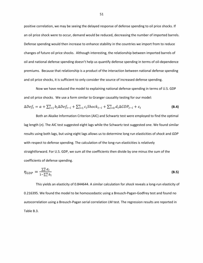
51  

positive correlation, we may be seeing the delayed response of defense spending to oil price shocks. If 

an oil price shock were to occur, demand would be reduced, decreasing the number of imported barrels.  

Defense spending would then increase to enhance stability in the countries we import from to reduce 

changes of future oil price shocks.  Although interesting, the relationship between imported barrels of 

oil and national defense spending doesn’t help us quantify defense spending in terms of oil‐dependence 

premiums.  Because that relationship is a product of the interaction between national defense spending 

and oil price shocks, it is sufficient to only consider the source of increased defense spending. 

Now we have reduced the model to explaining national defense spending in terms of U.S. GDP 

and oil price shocks.  We use a form similar to Granger causality testing for our model: 

∆𝐷𝑒𝑓D = 𝑎 + ∑ 𝑏\∆𝐷𝑒𝑓DK\]\^L + ∑ 𝑐\𝑆ℎ𝑜𝑐𝑘DK\]

\^L + ∑ 𝑑\∆𝐺𝐷𝑃DK\]\^+ + 𝜀D           (B.4) 

Both an Akaike Information Criterion (AIC) and Schwartz test were employed to find the optimal 

lag length (n). The AIC test suggested eight lags while the Schwartz test suggested one. We found similar 

results using both lags, but using eight lags allows us to determine long run elasticities of shock and GDP 

with respect to defense spending. The calculation of the long‐run elasticities is relatively 

straightforward. For U.S. GDP, we sum all the coefficients then divide by one minus the sum of the 

coefficients of defense spending.  

𝜂e%< = ∑ fghiLK∑ jghk

                         (B.5) 

This yields an elasticity of 0.844644. A similar calculation for shock reveals a long‐run elasticity of 

0.216395. We found the model to be homoscedastic using a Breusch‐Pagan‐Godfrey test and found no 

autocorrelation using a Breusch‐Pagan serial correlation LM test. The regression results are reported in 

Table B.3. 

   

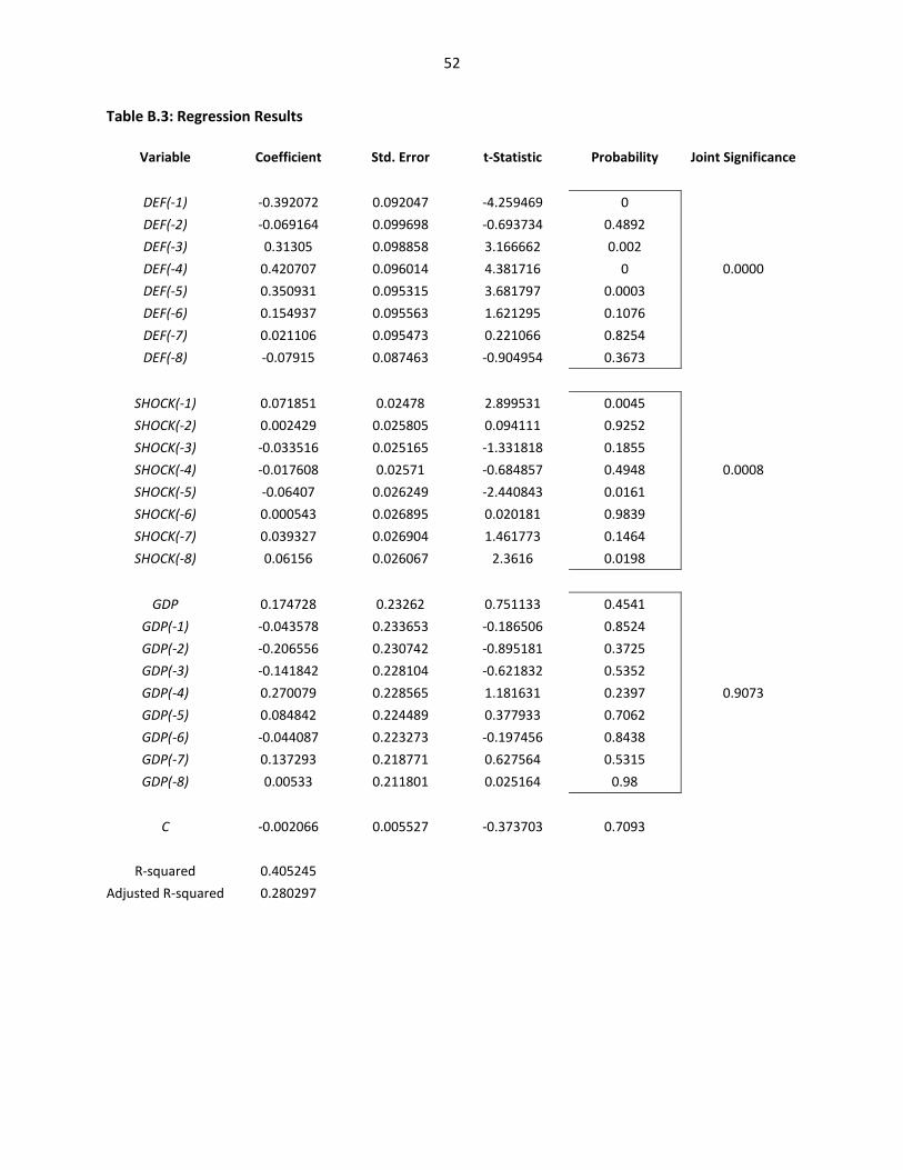
52  

Table B.3: Regression Results 

Variable  Coefficient  Std. Error  t‐Statistic  Probability    Joint Significance            

DEF(‐1)  ‐0.392072  0.092047  ‐4.259469  0   DEF(‐2)  ‐0.069164  0.099698  ‐0.693734  0.4892   DEF(‐3)  0.31305  0.098858  3.166662  0.002   DEF(‐4)  0.420707  0.096014  4.381716  0  0.0000 DEF(‐5)  0.350931  0.095315  3.681797  0.0003   DEF(‐6)  0.154937  0.095563  1.621295  0.1076   DEF(‐7)  0.021106  0.095473  0.221066  0.8254   DEF(‐8)  ‐0.07915  0.087463  ‐0.904954  0.3673   

           SHOCK(‐1)  0.071851  0.02478  2.899531  0.0045   SHOCK(‐2)  0.002429  0.025805  0.094111  0.9252   SHOCK(‐3)  ‐0.033516  0.025165  ‐1.331818  0.1855   SHOCK(‐4)  ‐0.017608  0.02571  ‐0.684857  0.4948  0.0008 SHOCK(‐5)  ‐0.06407  0.026249  ‐2.440843  0.0161   SHOCK(‐6)  0.000543  0.026895  0.020181  0.9839   SHOCK(‐7)  0.039327  0.026904  1.461773  0.1464   SHOCK(‐8)  0.06156  0.026067  2.3616  0.0198   

           GDP  0.174728  0.23262  0.751133  0.4541   

GDP(‐1)  ‐0.043578  0.233653  ‐0.186506  0.8524   GDP(‐2)  ‐0.206556  0.230742  ‐0.895181  0.3725   GDP(‐3)  ‐0.141842  0.228104  ‐0.621832  0.5352   GDP(‐4)  0.270079  0.228565  1.181631  0.2397  0.9073 GDP(‐5)  0.084842  0.224489  0.377933  0.7062   GDP(‐6)  ‐0.044087  0.223273  ‐0.197456  0.8438   GDP(‐7)  0.137293  0.218771  0.627564  0.5315   GDP(‐8)  0.00533  0.211801  0.025164  0.98   

            C  ‐0.002066  0.005527  ‐0.373703  0.7093              

R‐squared  0.405245         Adjusted R‐squared  0.280297          

 

   

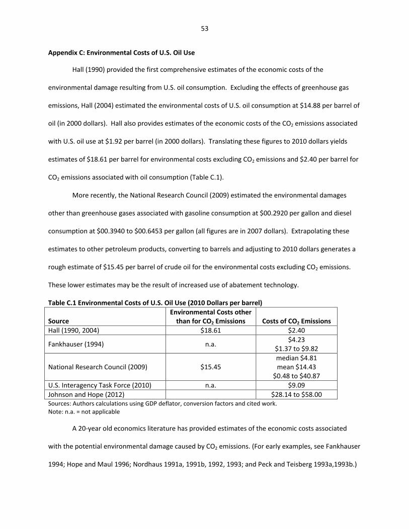
53  

Appendix C: Environmental Costs of U.S. Oil Use 

Hall (1990) provided the first comprehensive estimates of the economic costs of the 

environmental damage resulting from U.S. oil consumption.  Excluding the effects of greenhouse gas 

emissions, Hall (2004) estimated the environmental costs of U.S. oil consumption at $14.88 per barrel of 

oil (in 2000 dollars).  Hall also provides estimates of the economic costs of the CO2 emissions associated 

with U.S. oil use at $1.92 per barrel (in 2000 dollars).  Translating these figures to 2010 dollars yields 

estimates of $18.61 per barrel for environmental costs excluding CO2 emissions and $2.40 per barrel for 

CO2 emissions associated with oil consumption (Table C.1). 

More recently, the National Research Council (2009) estimated the environmental damages 

other than greenhouse gases associated with gasoline consumption at $00.2920 per gallon and diesel 

consumption at $00.3940 to $00.6453 per gallon (all figures are in 2007 dollars).  Extrapolating these 

estimates to other petroleum products, converting to barrels and adjusting to 2010 dollars generates a 

rough estimate of $15.45 per barrel of crude oil for the environmental costs excluding CO2 emissions.  

These lower estimates may be the result of increased use of abatement technology. 

Table C.1 Environmental Costs of U.S. Oil Use (2010 Dollars per barrel)  Source 

Environmental Costs other than for CO2 Emissions 

 Costs of CO2 Emissions 

Hall (1990, 2004)  $18.61  $2.40 

Fankhauser (1994)  n.a.  $4.23 $1.37 to $9.82 

National Research Council (2009)  $15.45 median $4.81 mean $14.43 

$0.48 to $40.87 U.S. Interagency Task Force (2010)  n.a.  $9.09 Johnson and Hope (2012)    $28.14 to $58.00 Sources: Authors calculations using GDP deflator, conversion factors and cited work. Note: n.a. = not applicable 

A 20‐year old economics literature has provided estimates of the economic costs associated 

with the potential environmental damage caused by CO2 emissions. (For early examples, see Fankhauser 

1994; Hope and Maul 1996; Nordhaus 1991a, 1991b, 1992, 1993; and Peck and Teisberg 1993a,1993b.) 

54  

Analysts and researchers working in the field must contend with a number of uncertainties: the extent 

to which these emissions will affect global warming, the environmental harm caused by global warming, 

and the economic costs of those environmental effects.  Discount rates also play an important role in 

these estimates.   

As reported by Brown and Huntington (1998), Hope and Maul (1996) find the worldwide 

marginal cost of CO2 emissions occurring in 2010 plausibly ranges from $0 to $270 per metric ton of 

carbon (in 1991 dollars) with a narrower range being more likely.  According to Brown and Huntington, 

Fankhauser’s estimates the most likely range from $7.40 to $52.90 per metric ton with a mean value of 

$22.80 (again in 1991 dollars).  Converting Fankhauser’s figures to 2010 dollars and applying them to the 

CO2 emissions associated with a barrel of oil yields estimates of $1.37 to $9.82 per barrel of oil with a 

mean value of $4.23 per barrel of oil. 

More recently, the National Research Council (2009) surveyed the climate literature and 

determined the worldwide marginal cost of CO2 emissions ranges from $0 to $100 per ton of CO2 with a 

range of $1 to $85 representing a 5 percent to 95 percent confidence interval (in 2007 dollars).  The 

median value is $10 per ton of CO2 and a mean value is $30 per ton.  Converting these estimates to 2010 

dollars and applying them to the CO2 emissions associated with a barrel of oil yields a plausible range of 

$0.00 to $48.08 per barrel of oil, a confidence band of $0.48 to $40.87 per barrel, a median value of 

$4.81 per barrel, and a mean value of $14.43 per barrel.   

Burtraw, Krupnick and Samson (2012) and Johnson and Hope (2012) report that a U.S. 

interagency task force (2010) estimated the mean social cost of carbon at $21 per ton of CO2 (2010 

dollars) for use in U.S. policy analysis, which translates to $9.09 per barrel of oil.  Using lower discount 

rates, equity weighting, and assumptions otherwise identical to those made by the interagency task 

force, Johnson and Hope estimate the social cost of CO2 emissions at $65 to $134 per ton of CO2, which 

translates to $28.14 to $58.00 per barrel of oil. 

55  

References 

Allaire, Maura and Stephen P. A. Brown. 2012. U.S. Energy Subsidies: Effects on Energy Markets and Carbon Dioxide Emissions. Pew Charitable Trusts, Washington, DC. (August 14). 

Atkins, Frank J. and S.M. Tayyebi Jazayeri. 2004. A Literature Review of Demand Studies in World Oil Markets. Department of Economics, Discussion Paper 2004‐7 (April). Calgary, AB: University of Calgary. 

Balke, Nathan S., Stephen P.A. Brown, and Mine K. Yücel. 2002. Oil Price Shocks and the U.S. Economy: Where Does the Asymmetry Originate? The Energy Journal 23(3): 27–52. 

Balke, Nathan S., Stephen P.A. Brown, and Mine K. Yücel. 2008. An International Perspective on Oil Price Shocks and U.S. Economic Activity. Globalization and Monetary Policy Institute Working Paper No. 20 (September). Dallas, TX: Federal Reserve Bank of Dallas. 

Barsky, Robert and Lutz Kilian. 2002. Do We Really Know that Oil Caused the Great Stagflation? A Monetary Alternative. NBER Macroeconomics Annual 2001 May: 137–183. 

Barsky, Robert and Lutz Kilian. 2004. Oil and the Macroeconomy since the 1970s. Journal of Economic Perspectives 18(4): 115–134. 

Beccue, Phillip and Hillard G. Huntington. 2005. Oil Disruption Risk Assessment. Energy Modeling Forum Special Report 8, August. Stanford, CA: Stanford University. 

Bernanke, Ben S., Mark Gertler, and Mark Watson. 1997. Systematic Monetary Policy and the Effects of Oil Price Shocks. Brookings Papers on Economic Activity 1997(1): 91–142. 

Blanchard, Olivier and J. Gali. 2007. The Macroeconomic Effects of Oil Price Shocks: Why Are the 2000s So Different from the 1970s? Department of Economics, Working Paper 07‐21 (August). Cambridge, MA: Massachusetts Institute of Technology. 

Bohi, Douglas R. 1989. Energy Price Shocks and Macroeconomic Performance. Washington, DC: Resources for the Future. 

Bohi, Douglas R. 1991. On the Macroeconomic Effects of Energy Price Shocks. Resources and Energy 13(2): 145–162.  

Bohi, Douglas R. and W. David Montgomery 1982a. Oil Prices, Energy Security, and Import Policy. Technical Report, Resources for the Future, Washington, DC.  

Bohi, Douglas R. and W. David Montgomery 1982b. Social Cost of Imported Oil and U.S. Import Policy. Annual Review of Energy 7:37‐60.  

Bohi, Douglas R. and Michael A. Toman. 1993. Energy Security: Externalities and Policies. Energy Policy 21(11): 1093–1109. 

Broadman, Harry G. 1986. The Social Cost of Imported Oil. Energy Policy 14(3): 242‐252. Broadman H.G. and W.W. Hogan 1988. Is and Oil Import Tariff Justified? An American Debate: The 

Numbers Say ‘Yes’. The Energy Journal 9: 7‐29. Brown, Stephen P. A. 1982. Reducing U.S. Vulnerability to World Oil Supply Disruptions. Economic 

Review, Federal Reserve Bank of Dallas (May). Brown, Stephen P.A. and Hillard G. Huntington. 2013. Assessing the U.S. Oil Security Premium. Energy 

Economics (accepted March 2013; in press). Brown, Stephen P.A. and Hillard G. Huntington. 2003. Terms of Trade and OECD Policies to Mitigate 

Global Climate Change. Economic and Financial Policy Review 2(1), Federal Reserve Bank of Dallas. 

Brown, Stephen P.A. and Hillard G. Huntington. 1998. Some Implications of Increased Cooperation in World Oil Conservation. Economic Review, Federal Reserve Bank of Dallas. Second Quarter. 

   

56  

Brown, Stephen P.A., Ryan T. Kennelly and Kylelar Maravich. 2012. An Examination of Selected Energy Tax Provisions: The Effect on Energy Markets and Carbon Dioxide Emissions, Report to the National Academy of Science. Center for Business and Economic Research, University of Nevada, Las Vegas. June 25. 

Brown, Stephen P.A. and Mine K. Yücel. 2002. Energy Prices and Aggregate Economic Activity: An Interpretative Survey. Quarterly Review of Economics and Finance 42(2): 193–208. 

Burtraw, Dallas, Alan Krupnick, and Gabriel Sampson. 2012. The True Cost of Electric Power. RFF Report, Resources for the Future, Washington, DC (June). 

Cooper, John C.B. 2003. Price Elasticity of Demand for Crude Oil: Estimates for 23 Countries. OPEC Review 27(1): 1‐8. March.  

Council on Foreign Relations. 2006. National Security Consequences of U.S. Oil Dependency. Independent Task Force Report No. 58, John Deutch and James R. Schlesinger (chairs) and David G. Victor (director). Washington, DC: Council on Foreign Relations Press. 

Dargay, Joyce. M., Dermot Gately, and Hillard G. Huntington. 2007. Price and Income Responsiveness of World Oil Demand, by Product. EMF OP 61, Energy Modeling Forum. Stanford, CA: Stanford University. 

Davis, Steven J. and John Haltiwanger. 2001. Sectoral Job Creation and Destruction Responses to Oil Price Changes and Other Shocks. Journal of Monetary Economics 48(3): 465‐512. December. 

EIA (Energy Information Administration). 2012. 2012 Annual Energy Outlook (revised). Washington, DC: EIA. 

EIA (Energy Information Administration). 2009. 2009 International Energy Outlook (revised). Washington, DC: EIA. 

Fankhauser, Samuel (1994), “The Social Costs of Greenhouse Emissions: An Expected Value Approach,” The Energy Journal 15 (2): 157–184.  

Ferderer, J. Peter. 1996. Oil Price Volatility and the Macroeconomy: A Solution to the Asymmetry Puzzle. Journal of Macroeconomics 18(1): 1–16. Winter. 

Finn, Mary G. 2000. Perfect Competition and the Effects of Energy Price Increases on Economic Activity. Journal of Money, Credit, and Banking 32(3): 400–416. 

Gately, Dermot and Hillard Huntington. 2002. The Asymmetric Effects of Changes in Price and Income on Energy and Oil Demand. The Energy Journal 23(1): 19–55. 

Greene, David L. 2011. Energy Security, Oil Dependence and Oil Independence: Is it OPEC or is it US? Presentation at OPEC at 50, a conference organized by the National Energy Policy Institute, Tulsa, Oklahoma (March). 

Greene, David L. 2010. Measuring Energy Security: Can the United States Achieve Oil Independence? Energy Policy 38: 1614‐1621. 

Greene, David L., Paul N. Leiby, Philip D. Patterson, Steven E. Plotkin, and Margaret K. Singh. 2007. Oil Independence: Achievable National Goal or Empty Slogan? Paper presented at Transportation Research Board Annual Meeting. Washington, DC, (January 21–25). 

Hall, Darwin C. 2004. External Costs of Energy. In Encyclopedia of Energy, vol 2, edited by Cutler J. Cleveland. Amsterdam/The Netherlands: Elsevier–Academic Press, 651–667. 

Hall, Darwin C. 1992. Oil and National Security. Energy Policy, 20(11): 1089‐1096. Hall, Darwin C. 1990. Preliminary Estimates of Cumulative Private and External Costs of Energy. 

Contemporary Policy Issues 8(3): 283‐307. Hamilton, James D. 1996. This Is What Happened to the Oil Price Macroeconomy Relationship. Journal of 

Monetary Economics 38(2): 215–220. Hamilton, James D. 2003. What Is an Oil Shock? Journal of Econometrics 113(2): 363–398. April. Hamilton, James D. 2009. Causes and Consequences of the Oil Shock 2007–2008. Brookings Papers on 

Economic Activity. pp. 215‐261. Spring. 

57  

Hamilton, James D. 2010. Nonlinearities and the Macroeconomic Effects of Oil Prices (Revised). Working Paper, University of California, San Diego. December. (forthcoming Macroeconomic Dynamics) 

Hickman, Bert, Hillard Huntington, and James Sweeney (eds.). 1987. Macroeconomic Impacts of Energy Shocks. Amsterdam: North‐Holland. 

Hope, Chris and Phillip Maul. 1996. Valuing the Impact of CO2 Emissions.  Energy Policy 24: 211–19.  Huntington, Hillard G. 2003. Energy Disruptions, Interfirm Price Effects and the Aggregate Economy. 

Energy Economics 25(2): 119–136. Huntington, Hillard G. 2005. The Economic Consequences of Higher Crude Oil Prices. Energy Modeling 

Special Report 9 (October). Stanford, CA: Stanford University. John, A. Andrew. 1995. Macroeconomic Externalities. In The New Macroeconomics: Imperfect 

Competition and Policy Effectiveness, edited by H. Dixon and N. Rankin. Cambridge, United Kingdom: Cambridge University Press, 139‐170. 

Jones, Donald W., Paul N. Leiby, and Inja K. Paik. 2004. Oil Price Shocks and the Macroeconomy: What Has Been Learned since 1996? The Energy Journal 25(2): 1‐32.  

Johnson, Laurie T. and Chris Hope. 2012. The Social Cost of Carbon in U.S. Regulatory Impact Analyses: an Introduction and Critique. Journal of Environmental Studies and Sciences 2(3): 205‐221. 

Kilian, Lutz. 2008. The Economic Effects of Energy Price Shocks. Journal of Economic Literature 46(4): 871–909. 

Kilian, Lutz. 2009. Not All Oil Price Shocks Are Alike: Disentangling Demand and Supply Shocks in the Crude Oil Market. American Economic Review 99(3): 1053–1069. 

Landsberg, Hans H. et al. 1979. Energy: The Next Twenty Years. Ballinger, Cambridge, MA. Leiby, Paul N. 2007. Estimating the Energy Security Benefits of Reduced U.S. Oil Imports. Oak Ridge 

National Laboratory Report ORNL/TM‐2007/028, revised (July 23). Oak Ridge, TN: Oak Ridge National Laboratory. 

McKinsey and Company. 2009. Unlocking Energy Efficiency in the U.S. Economy (July). Mork, Knut Anton. 1989. Oil and the Macroeconomy, When Prices Go Up and Down: An Extension of 

Hamilton’s Results. Journal of Political Economy 97(3): 740–744. June. National Research Council. 2009. Hidden Costs of Energy: Unpriced Consequences of Energy Production 

and Use. National Academy of Science, Washington, DC. Nordhaus, William D. 2009. The Economics of an Integrated World Oil Market. Paper presented at the 

International Energy Workshop, June 2009, Vienna, Italy. Nordhaus, William D. 1993. Reflections on the Economics of Climate Change. Journal of Economic 

Perspectives (7)4: 11‐25. Nordhaus, William D. 1991a. To Slow or Not to Slow: The Economics of Global Warming. Economic 

Journal 101 (July): 920 –37. Nordhaus, William D. 1991b. A Sketch of the Economics of the Greenhouse Effect. American Economic 

Review 81 (May, Papers and Proceedings): 920 – 37. Nordhaus, William D.  1992. The DICE Model: Background and Structure of a Dynamic Integrated Climate 

Economy Model of the Economics of Global Warming. Cowles Foundation Discussion Paper no. 1009, New Haven, Connecticut (February). 

Parry, Ian W.H. and Joel Darmstadter. 2003. The Cost of U.S. Oil Dependency. Discussion paper 03‐59. Resources for the Future, Washington, DC. (December). 

Peck, Stephen C. and Thomas J. Teisberg. 1992. CETA: A Model for Carbon Emissions Trajectory Assessment. The Energy Journal 13 (1): 55 –77. 

Peck, Stephen C. and Thomas J. Teisberg. 1993a. CO2 Emissions Control: Comparing Policy Instruments. Energy Policy 21: 222–30. 

Peck, Stephen C. and Thomas J. Teisberg. 1993b. Global Warming Uncertainties and the Value of Information: An Analysis Using CETA,” Resource and Energy Economics 15 (March): 71– 97. 

58  

Rotemberg, Julio, and Michael Woodford. 1996. Imperfect Competition and the Effects of Energy Price Increases on Economic Activity. Journal of Money, Credit and Banking 28(4): 549–577. 

Schultze, Charles L. 1977. The Public Use of Private Interest. Washington, DC: The Brookings Institution. Smith, James L. 2009. World Oil: Market or Mayhem. Journal of Economic Perspectives, 23(3): 145–164. Toman, Michael A. 1993. "The Economics of Energy Security: Theory, Evidence, Policy," Handbook of 

Natural Resource and Energy Economics, vol. III, edited by A.V. Kneese and J.L. Sweeney, Chapter 25, pp. 1167‐1218, New York: Elsevier Science Publishers B.V. 

U.S. Government (2010) Interagency Working Group on Social Cost of Carbon. Technical support document: social cost of carbon for regulatory impact analysis under Executive Order 12866.