Master of Science Thesis in Information CodingDepartment of Electrical Engineering, Linköping University, 2016

Comparison ofTechnologies forGeneral-PurposeComputing on GraphicsProcessing Units

Torbjörn Sörman

Master of Science Thesis in Information Coding

Comparison of Technologies for General-Purpose Computing on GraphicsProcessing Units

Torbjörn Sörman

LiTH-ISY-EX–16/4923–SE

Supervisor: Robert Forchheimerisy, Linköpings universitet

Åsa DetterfeltMindRoad AB

Examiner: Ingemar Ragnemalmisy, Linköpings universitet

Organisatorisk avdelningDepartment of Electrical Engineering

Linköping UniversitySE-581 83 Linköping, Sweden

Copyright © 2016 Torbjörn Sörman

Abstract

The computational capacity of graphics cards for general-purpose computinghave progressed fast over the last decade. A major reason is computational heavycomputer games, where standard of performance and high quality graphics con-stantly rise. Another reason is better suitable technologies for programming thegraphics cards. Combined, the product is high raw performance devices andmeans to access that performance. This thesis investigates some of the currenttechnologies for general-purpose computing on graphics processing units. Tech-nologies are primarily compared by means of benchmarking performance andsecondarily by factors concerning programming and implementation. The choiceof technology can have a large impact on performance. The benchmark applica-tion found the difference in execution time of the fastest technology, CUDA, com-pared to the slowest, OpenCL, to be twice a factor of two. The benchmark applica-tion also found out that the older technologies, OpenGL and DirectX, are compet-itive with CUDA and OpenCL in terms of resulting raw performance.

iii

Acknowledgments

I would like to thank Åsa Detterfelt for the opportunity to make this thesis workat MindRoad AB. I would also like to thank Ingemar Ragnemalm at ISY.

Linköping, Februari 2016Torbjörn Sörman

v

Contents

List of Tables ix

List of Figures xi

Acronyms xiii

1 Introduction 11.1 Background . . . . . . . . . . . . . . . . . . . . . . . . . . . . . . . 11.2 Problem statement . . . . . . . . . . . . . . . . . . . . . . . . . . . 21.3 Purpose and goal of the thesis work . . . . . . . . . . . . . . . . . . 21.4 Delimitations . . . . . . . . . . . . . . . . . . . . . . . . . . . . . . . 2

2 Benchmark algorithm 32.1 Discrete Fourier Transform . . . . . . . . . . . . . . . . . . . . . . . 3

2.1.1 Fast Fourier Transform . . . . . . . . . . . . . . . . . . . . . 42.2 Image processing . . . . . . . . . . . . . . . . . . . . . . . . . . . . 42.3 Image compression . . . . . . . . . . . . . . . . . . . . . . . . . . . 42.4 Linear algebra . . . . . . . . . . . . . . . . . . . . . . . . . . . . . . 52.5 Sorting . . . . . . . . . . . . . . . . . . . . . . . . . . . . . . . . . . 5

2.5.1 Efficient sorting . . . . . . . . . . . . . . . . . . . . . . . . . 62.6 Criteria for Algorithm Selection . . . . . . . . . . . . . . . . . . . . 6

3 Theory 73.1 Graphics Processing Unit . . . . . . . . . . . . . . . . . . . . . . . . 7

3.1.1 GPGPU . . . . . . . . . . . . . . . . . . . . . . . . . . . . . . 73.1.2 GPU vs CPU . . . . . . . . . . . . . . . . . . . . . . . . . . . 8

3.2 Fast Fourier Transform . . . . . . . . . . . . . . . . . . . . . . . . . 93.2.1 Cooley-Tukey . . . . . . . . . . . . . . . . . . . . . . . . . . 93.2.2 Constant geometry . . . . . . . . . . . . . . . . . . . . . . . 103.2.3 Parallelism in FFT . . . . . . . . . . . . . . . . . . . . . . . . 103.2.4 GPU algorithm . . . . . . . . . . . . . . . . . . . . . . . . . 10

3.3 Related research . . . . . . . . . . . . . . . . . . . . . . . . . . . . . 12

vii

viii Contents

4 Technologies 154.1 CUDA . . . . . . . . . . . . . . . . . . . . . . . . . . . . . . . . . . . 154.2 OpenCL . . . . . . . . . . . . . . . . . . . . . . . . . . . . . . . . . . 164.3 DirectCompute . . . . . . . . . . . . . . . . . . . . . . . . . . . . . 184.4 OpenGL . . . . . . . . . . . . . . . . . . . . . . . . . . . . . . . . . 194.5 OpenMP . . . . . . . . . . . . . . . . . . . . . . . . . . . . . . . . . 194.6 External libraries . . . . . . . . . . . . . . . . . . . . . . . . . . . . 20

5 Implementation 215.1 Benchmark application GPU . . . . . . . . . . . . . . . . . . . . . . 21

5.1.1 FFT . . . . . . . . . . . . . . . . . . . . . . . . . . . . . . . . 215.1.2 FFT 2D . . . . . . . . . . . . . . . . . . . . . . . . . . . . . . 245.1.3 Differences . . . . . . . . . . . . . . . . . . . . . . . . . . . . 26

5.2 Benchmark application CPU . . . . . . . . . . . . . . . . . . . . . . 295.2.1 FFT with OpenMP . . . . . . . . . . . . . . . . . . . . . . . 295.2.2 FFT 2D with OpenMP . . . . . . . . . . . . . . . . . . . . . 305.2.3 Differences with GPU . . . . . . . . . . . . . . . . . . . . . . 30

5.3 Benchmark configurations . . . . . . . . . . . . . . . . . . . . . . . 315.3.1 Limitations . . . . . . . . . . . . . . . . . . . . . . . . . . . . 315.3.2 Testing . . . . . . . . . . . . . . . . . . . . . . . . . . . . . . 315.3.3 Reference libraries . . . . . . . . . . . . . . . . . . . . . . . 31

6 Evaluation 336.1 Results . . . . . . . . . . . . . . . . . . . . . . . . . . . . . . . . . . 33

6.1.1 Forward FFT . . . . . . . . . . . . . . . . . . . . . . . . . . . 346.1.2 FFT 2D . . . . . . . . . . . . . . . . . . . . . . . . . . . . . . 38

6.2 Discussion . . . . . . . . . . . . . . . . . . . . . . . . . . . . . . . . 426.2.1 Qualitative assessment . . . . . . . . . . . . . . . . . . . . . 446.2.2 Method . . . . . . . . . . . . . . . . . . . . . . . . . . . . . . 45

6.3 Conclusions . . . . . . . . . . . . . . . . . . . . . . . . . . . . . . . 466.3.1 Benchmark application . . . . . . . . . . . . . . . . . . . . . 466.3.2 Benchmark performance . . . . . . . . . . . . . . . . . . . . 476.3.3 Implementation . . . . . . . . . . . . . . . . . . . . . . . . . 47

6.4 Future work . . . . . . . . . . . . . . . . . . . . . . . . . . . . . . . 486.4.1 Application . . . . . . . . . . . . . . . . . . . . . . . . . . . 486.4.2 Hardware . . . . . . . . . . . . . . . . . . . . . . . . . . . . 48

Bibliography 51

List of Tables

3.1 Global kernel parameter list with argument depending on size ofinput N and stage. . . . . . . . . . . . . . . . . . . . . . . . . . . . 11

3.2 Local kernel parameter list with argument depending on size ofinput N and number of stages left to complete. . . . . . . . . . . . 12

4.1 Table of function types in CUDA. . . . . . . . . . . . . . . . . . . . 16

5.1 Shared memory size in bytes, threads and block configuration perdevice. . . . . . . . . . . . . . . . . . . . . . . . . . . . . . . . . . . 22

5.2 Integer intrinsic bit-reverse function for different technologies. . . 245.3 Table illustrating how to set parameters and launch a kernel. . . . 285.4 Synchronization in GPU technologies. . . . . . . . . . . . . . . . . 295.5 Twiddle factors for a 16-point sequence where α equals (2 ·π)/16.

Each row i corresponds to the ith butterfly operation. . . . . . . . 305.6 Libraries included to compare with the implementation. . . . . . . 31

6.1 Technologies included in the experimental setup. . . . . . . . . . . 346.2 Table comparing CUDA to CPU implementations. . . . . . . . . . 47

ix

x LIST OF TABLES

List of Figures

3.1 The GPU uses more transistors for data processing . . . . . . . . . 83.2 Radix-2 butterfly operations . . . . . . . . . . . . . . . . . . . . . . 93.3 8-point radix-2 FFT using Cooley-Tukey algorithm . . . . . . . . . 93.4 Flow graph of an radix-2 FFT using the constant geometry algo-

rithm. . . . . . . . . . . . . . . . . . . . . . . . . . . . . . . . . . . . 10

4.1 CUDA global kernel . . . . . . . . . . . . . . . . . . . . . . . . . . . 164.2 OpenCL global kernel . . . . . . . . . . . . . . . . . . . . . . . . . . 174.3 DirectCompute global kernel . . . . . . . . . . . . . . . . . . . . . 184.4 OpenGL global kernel . . . . . . . . . . . . . . . . . . . . . . . . . . 194.5 OpenMP procedure completing one stage . . . . . . . . . . . . . . 20

5.1 Overview of the events in the algorithm. . . . . . . . . . . . . . . . 215.2 Flow graph of a 16-point FFT using (stage 1 and 2) Cooley-Tukey

algorithm and (stage 3 and 4) constant geometry algorithm. Thesolid box is the bit-reverse order output. Dotted boxes are separatekernel launches, dashed boxes are data transfered to local memorybefore computing the remaining stages. . . . . . . . . . . . . . . . 23

5.3 CUDA example code showing index calculation for each stage inthe global kernel, N is the total number of points. io_low is theindex of the first input in the butterfly operation and io_high theindex of the second. . . . . . . . . . . . . . . . . . . . . . . . . . . . 23

5.4 CUDA code for index calculation of points in shared memory. . . 245.5 Code returning a bit-reversed unsigned integer where x is the in-

put. Only 32-bit integer input and output. . . . . . . . . . . . . . 245.6 Original image in 5.6a transformed and represented with a quad-

rant shifted magnitude visualization (scale skewed for improvedillustration) in 5.6b. . . . . . . . . . . . . . . . . . . . . . . . . . . 25

5.7 CUDA device code for the transpose kernel. . . . . . . . . . . . . . 265.8 Illustration of how shared memory is used in transposing an image.

Input data is tiled and each tile is written to shared memory andtransposed before written to the output memory. . . . . . . . . . . 27

5.9 An overview of the setup phase for the GPU technologies. . . . . . 275.10 OpenMP implementation overview transforming sequence of size

N . . . . . . . . . . . . . . . . . . . . . . . . . . . . . . . . . . . . . . 29

xi

xii LIST OF FIGURES

5.11 C/C++ code performing the bit-reverse ordering of a N-point se-quence. . . . . . . . . . . . . . . . . . . . . . . . . . . . . . . . . . . 30

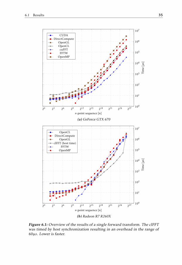
6.1 Overview of the results of a single forward transform. The clFFTwas timed by host synchronization resulting in an overhead in therange of 60µs. Lower is faster. . . . . . . . . . . . . . . . . . . . . . 35

6.2 Performance relative CUDA implementation in 6.2a and OpenCLin 6.2b. Lower is better. . . . . . . . . . . . . . . . . . . . . . . . . . 36

6.3 Performance relative CUDA implementation on GeForce GTX 670and Intel Core i7 3770K 3.5GHz CPU. . . . . . . . . . . . . . . . . 37

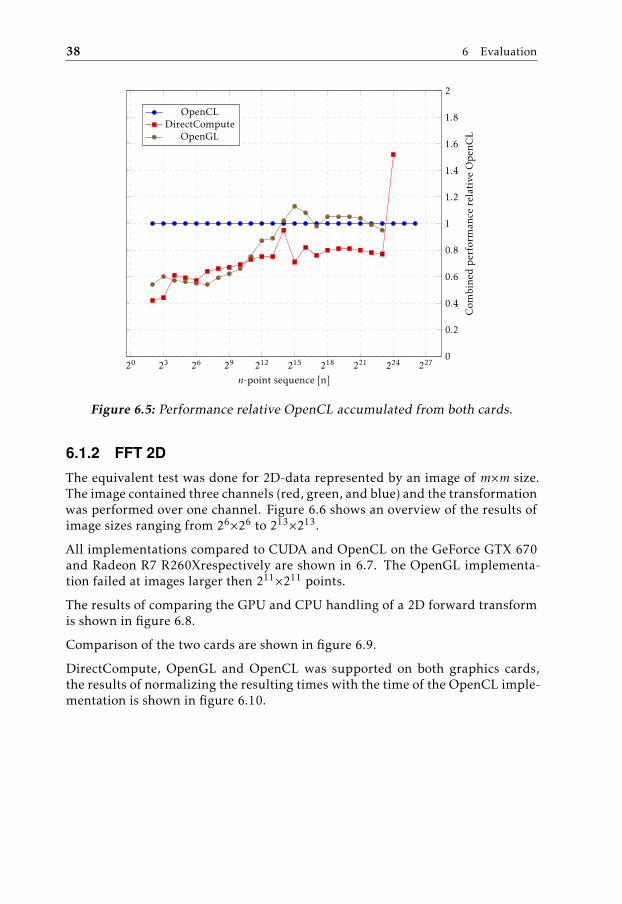
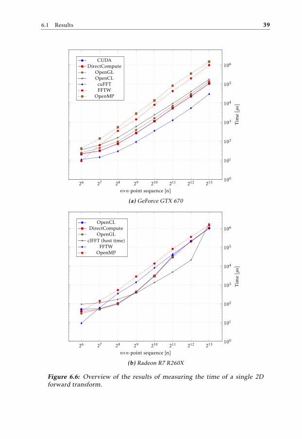
6.4 Comparison between Radeon R7 R260X and GeForce GTX 670. . . 376.5 Performance relative OpenCL accumulated from both cards. . . . 386.6 Overview of the results of measuring the time of a single 2D for-

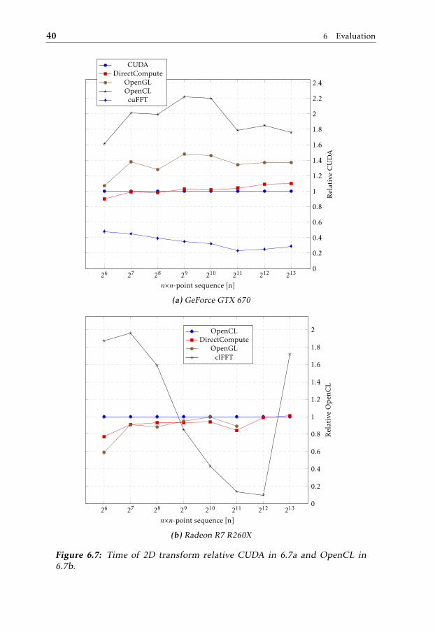
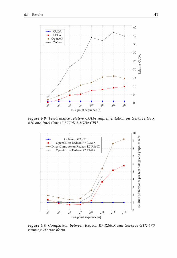
ward transform. . . . . . . . . . . . . . . . . . . . . . . . . . . . . . 396.7 Time of 2D transform relative CUDA in 6.7a and OpenCL in 6.7b. 406.8 Performance relative CUDA implementation on GeForce GTX 670

and Intel Core i7 3770K 3.5GHz CPU. . . . . . . . . . . . . . . . . 416.9 Comparison between Radeon R7 R260X and GeForce GTX 670 run-

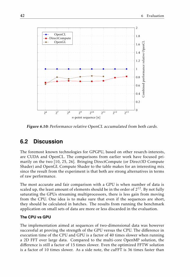
ning 2D transform. . . . . . . . . . . . . . . . . . . . . . . . . . . . 416.10 Performance relative OpenCL accumulated from both cards. . . . 42

Acronyms

1D One-dimensional.

2D Two-dimensional.

3D Three-dimensional.

ACL AMD Compute Libraries.

API Application Programming Interface.

BLAS Basic Linear Algebra Subprograms.

CPU Central Processing Unit.

CUDA Compute Unified Device Architecture.

DCT Discrete Cosine Transform.

DFT Discrete Fourier Transform.

DIF Decimation-In-Frequency.

DWT Discrete Wavelet Transform.

EBCOT Embedded Block Coding with Optimized Truncation.

FFT Fast Fourier Transform.

FFTW Fastest Fourier Transform in the West.

FLOPS Floating-point Operations Per Second.

FPGA Field-Programmable Gate Array.

GCN Graphics Core Next.

xiii

xiv Acronyms

GLSL OpenGL Shading Language.

GPGPU General-Purpose computing on Graphics Processing Units.

GPU Graphics Processing Unit.

HBM High Bandwidth Memory.

HBM2 High Bandwidth Memory.

HLSL High-Level Shading Language.

HPC High-Performance Computing.

ILP Instruction-Level Parallelism.

OpenCL Open Computing Language.

OpenGL Open Graphics Library.

OpenMP Open Multi-Processing.

OS Operating System.

PTX Parallel Thread Execution.

RDP Remote Desktop Protocol.

SM Streaming Multiprocessor.

VLIW Very Long Instruction Word-processor.

1Introduction

This chapter gives an introduction to the thesis. The background, purpose andgoal of the thesis, describes a list of abbreviations and the structure of this report.

1.1 Background

Technical improvements of hardware has for a long period of time been the bestway to solve computationally demanding problems faster. However, during thelast decades, the limit of what can be achieved by hardware improvements appearto have been reached: The operating frequency of the Central Processing Unit(CPU) does no longer significantly improve. Problems relying on single threadperformance are limited by three primary technical factors:

1. The Instruction-Level Parallelism (ILP) wall

2. The memory wall

3. The power wall

The first wall states that it is hard to further exploit simultaneous CPU instruc-tions: techniques such as instruction pipelining, superscalar execution and VeryLong Instruction Word-processor (VLIW) exists but complexity and latency ofhardware reduces the benefits.

The second wall, the gap between CPU speed and memory access time, that maycost several hundreds of CPU cycles if accessing primary memory.

The third wall is the power and heating problem. The power consumed is in-creased exponentially with each factorial increase of operating frequency.

1

2 1 Introduction

Improvements can be found in exploiting parallelism. Either the problem itselfis already inherently parallelizable, or reconstruct the problem. This trend mani-fests in development towards use and construction of multi-core microprocessors.The Graphics Processing Unit (GPU) is one such device, it originally exploitedthe inherent parallelism within visual rendering but now is available as a tool formassively parallelizable problems.

1.2 Problem statement

Programmers might experience a threshold and a slow learning curve to movefrom a sequential to a thread-parallel programming paradigm that is GPU pro-gramming. Obstacles involve learning about the hardware architecture, and re-structure the application. Knowing the limitations and benefits might even pro-vide reason to not utilize the GPU, and instead choose to work with a multi-coreCPU.

Depending on ones preferences, needs, and future goals; selecting one technologyover the other can be very crucial for productivity. Factors concerning productiv-ity can be portability, hardware requirements, programmability, how well it in-tegrates with other frameworks and Application Programming Interface (API)s,or how well it is supported by the provider and developer community. Withinthe range of this thesis, the covered technologies are Compute Unified Device Ar-chitecture (CUDA), Open Computing Language (OpenCL), DirectCompute (APIwithin DirectX), and Open Graphics Library (OpenGL) Compute Shaders.

1.3 Purpose and goal of the thesis work

The purpose of this thesis is to evaluate, select, and implement an applicationsuitable for General-Purpose computing on Graphics Processing Units (GPGPU).

To implement the same application in technologies for GPGPU: (CUDA, OpenCL,DirectCompute, and OpenGL), compare GPU results with results from an sequen-tial C/C++ implementation and a multi-core OpenMP implementation, and tocompare the different technologies by means of benchmarking, and the goal is tomake qualitative assessments of how it is to use the technologies.

1.4 Delimitations

Only one benchmark application algorithm will be selected, the scope and timerequired only allows for one algorithm to be tested. Each technology have differ-ent debugging and profiling tools and those are not included in the comparisonof the technologies. However important such tool can be, they are of a subjectivenature and more difficult to put a measure on.

2Benchmark algorithm

This part cover a possible applications for a GPGPU study. The basic theoryand motivation why they are suitable for benchmarking GPGPU technologies ispresented.

2.1 Discrete Fourier Transform

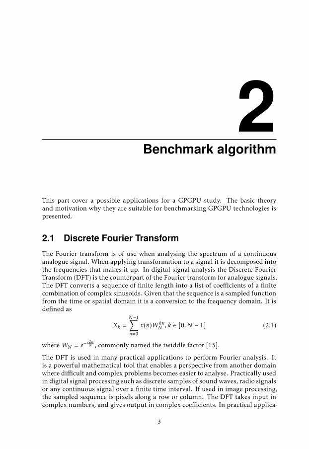
The Fourier transform is of use when analysing the spectrum of a continuousanalogue signal. When applying transformation to a signal it is decomposed intothe frequencies that makes it up. In digital signal analysis the Discrete FourierTransform (DFT) is the counterpart of the Fourier transform for analogue signals.The DFT converts a sequence of finite length into a list of coefficients of a finitecombination of complex sinusoids. Given that the sequence is a sampled functionfrom the time or spatial domain it is a conversion to the frequency domain. It isdefined as

Xk =N−1∑n=0

x(n)W knN , k ∈ [0, N − 1] (2.1)

where WN = e−i2πN , commonly named the twiddle factor [15].

The DFT is used in many practical applications to perform Fourier analysis. Itis a powerful mathematical tool that enables a perspective from another domainwhere difficult and complex problems becomes easier to analyse. Practically usedin digital signal processing such as discrete samples of sound waves, radio signalsor any continuous signal over a finite time interval. If used in image processing,the sampled sequence is pixels along a row or column. The DFT takes input incomplex numbers, and gives output in complex coefficients. In practical applica-

3

4 2 Benchmark algorithm

tions the input is usually real numbers.

2.1.1 Fast Fourier Transform

The problem with the DFT is that the direct computation require O(nn) complexmultiplications and complex additions, which makes it computationally heavyand impractical in high throughput applications. The Fast Fourier Transform(FFT) is one of the most common algorithms used to compute the DFT of a se-quence. A FFT computes the transformation by factorizing the transformationmatrix of the DFT into a product of mostly zero factors. This reduces the orderof computations to O(n log n) complex multiplications and additions.

The FFT was made popular in 1965 [7] by J.W Cooley and John Tukey. It found itis way into practical use at the same time, and meant a serious breakthroughin digital signal processing [8, 5]. However, the complete algorithm was notinvented at the time. The history of the Cooley-Tukey FFT algorithm can betraced back to around 1805 by work of the famous mathematician Carl FriedrichGauss[18]. The algorithm is a divide-and-conquer algorithm that relies on recur-sively dividing the input into sub-blocks. Eventually the problem is small enoughto be solved, and the sub-blocks are combined into the final result.

2.2 Image processing

Image processing consists of a wide range of domains. Earlier academic workwith performance evaluation on the GPU [25] tested four major domains andcompared them with the CPU. The domains were Three-dimensional (3D) shapereconstruction, feature extraction, image compression, and computational pho-tography. Image processing is typically favourable on a GPU since images areinherently a parallel structure.

Most image processing algorithms apply the same computation on a number ofpixels, and that typically is a data-parallel operation. Some algorithms can thenbe expected to have huge speed-up compared to an efficient CPU implementation.A representative task is applying a simple image filter that gathers neighbouringpixel-values and compute a new value for a pixel. If done with respect to theunderlying structure of the system, one can expect a speed-up near linear to thenumber of computational cores used. That is, a CPU with four cores can theoret-ically expect a near four time speed-up compared to a single core. This extendsto a GPU so that a GPU with n cores can expect a speed-up in the order of n inideal cases. An example of this is a Gaussian blur (or smoothing) filter.

2.3 Image compression

The image compression standard JPEG2000 offers algorithms with parallelismbut is very computationally and memory intensive. The standard aims to im-prove performance over JPEG, but also to add new features. The following sec-

2.4 Linear algebra 5

tions are part of the JPEG2000 algorithm [6]:

1. Color Component transformation

2. Tiling

3. Wavelet transform

4. Quantization

5. Coding

The computation heavy parts can be identified as the Discrete Wavelet Transform(DWT) and the encoding engine uses Embedded Block Coding with OptimizedTruncation (EBCOT) Tier-1.

One difference between the older format JPEG and the newer JPEG2000 is theuse of DWT instead of Discrete Cosine Transform (DCT). In comparison to theDFT, the DCT operates solely on real values. DWTs, on the other hand, usesanother representation that allows for a time complexity of O(N ).

2.4 Linear algebra

Linear algebra is central to both pure and applied mathematics. In scientific com-puting it is a highly relevant problem to solve dense linear systems efficiently. Inthe initial uses of GPUs in scientific computing, the graphics pipeline was suc-cessfully used for linear algebra through programmable vertex and pixel shaders[20]. Methods and systems used later on for utilizing GPUs have been shownefficient also in hybrid systems (multi-core CPUs + GPUs) [27]. Linear algebrais highly suitable for GPUs and with careful calibration it is possible to reach80%-90% of the theoretical peak speed of large matrices [28].

Common operations are vector addition, scalar multiplication, dot products, lin-ear combinations, and matrix multiplication. Matrix multiplications have a hightime complexity, O(N3), which makes it a bottleneck in many algorithms. Matrixdecomposition like LU, QR, and Cholesky decomposition are used very often andare subject for benchmark applications targeting GPUs [28].

2.5 Sorting

The sort operation is an important part of computer science and is a classic prob-lem to work on. There exists several sorting techniques, and depending on prob-lem and requirements a suitable algorithm is found by examining the attributes.

Sorting algorithms can be organized into two categories, data-driven and data-independent. The quicksort algorithm is a well known example of a data-drivensorting algorithm. It performs with time complexity O(n log n) on average, buthave a time complexity of O(n2) in the worst case. Another data-driven algorithmthat does not have this problem is the heap sort algorithm, but it suffers from

6 2 Benchmark algorithm

difficult data access patterns instead. Data-driven algorithms are not the easiestto parallelize since their behaviour is unknown and may cause bad load balancingamong computational units.

The data independent algorithms is the algorithms that always perform the sameprocess no matter what the data. This behaviour makes them suitable for im-plementation on multiple processors, and fixed sequences of instructions, wherethe moment in which data is synchronized and communication must occur areknown in advance.

2.5.1 Efficient sorting

Bitonic sort have been used early on in the utilization of GPUs for sorting. Eventhough it has the time complexity of O(n log n2) it has been an easy way of doinga reasonably efficient sort on GPUs. Other high-performance sorting on GPUsare often combinations of algorithms. Some examples of combined sort methodson GPUs are the bitonic merge sort, and a bucket sort that split the sequence intosmaller sequences before each being sorted with a merge sort.

A popular algorithm for GPUs have been variants of radix sort which is a non-comparative integer sorting algorithm. Radix sorts can be described as beingeasy to implement and still as efficient as more sophisticated algorithms. Radixsort works by grouping the integer keys by the individual digit value in the samesignificant position and value.

2.6 Criteria for Algorithm Selection

A benchmarking application is sought that have the necessary complexity and rel-evance for both practical uses and the scientific community. The algorithm withenough complexity and challenges is the FFT. Compared to the other presentedalgorithms the FFT is more complex than the matrix operations and the regularsorting algorithms. The FFT does not demand as much domain knowledge as theimage compression algorithms, but it is still a very important algorithm for manyapplications.

The difficulties of working with multi-core systems are applied to GPUs. WhatGPUs are missing compared to multi-core CPUs, is the power of working in se-quential. Instead, GPUs are excellent at fast context switching and hiding mem-ory latencies. Most effort of working with GPUs extends to supply tasks withenough parallelism, avoiding branching, and optimize memory access patterns.One important issue is also the host to device memory transfer-time. If the algo-rithm is much faster on the GPU, a CPU could still be faster if the host to deviceand back transfer is a large part of the total time.

By selecting an algorithm that have much scientific interest and history relevantcomparisons can be made. It is sufficient to say that one can demand a reason-able performance by utilizing information sources showing implementations onGPUs.

3Theory

This chapter will give an introduction to the FFT algorithm and a brief introduc-tion of the GPU.

3.1 Graphics Processing Unit

A GPU is traditionally specialized hardware for efficient manipulation of com-puter graphics and image processing [24]. The inherent parallel structure of im-ages and graphics makes them very efficient at some general problems whereparallelism can be exploited. The concept of GPGPU is solving a problem on theGPU platform instead of a multi-core CPU system.

3.1.1 GPGPU

In the early days of GPGPU one had to know a lot about computer graphics tocompute general data. The available APIs were created for graphics processing.The dominant APIs were OpenGL and DirectX. High-Level Shading Language(HLSL) and OpenGL Shading Language (GLSL) made the step easier, but it stillgenerated code into the APIs.

A big change was when NVIDIA released CUDA, which together with new hard-ware made it possible to use standard C-code to program the GPU (with a few ex-tensions). Parallel software and hardware was a small market at the time, and thesimplified use of the GPU for parallel tasks opened up to many new customers.However, the main business is still graphics and the manufacturers can not makecards too expensive, especially at the cost of graphics performance (as would in-crease of more double-precision floating-point capacity). This can be exemplifiedwith a comparison between NVIDIA’s Maxwell micro architecture, and the prede-

7

8 3 Theory

ctrl

Cache

ALU ALU

ALU ALU

DRAM DRAM

CPU GPU

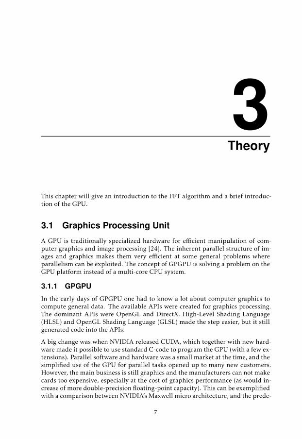
Figure 3.1: The GPU uses more transistors for data processing

cessor Kepler: Both are similar, but with Maxwell some of the double-precisionfloating-point capacity was removed in favour of single-precision floating-pointvalue capacity (preferred in graphics).

Using GPUs in the context of data centers and High-Performance Computing(HPC), studies show that GPU acceleration can reduce power [19] and it is rele-vant to know the behaviour of the GPUs in the context of power and HPC [16]for the best utilization.

3.1.2 GPU vs CPU

The GPU is built on a principle of more execution units instead of higher clock-frequency to improve performance. Comparing the CPU with the GPU, theGPU performs a much higher theoretical Floating-point Operations Per Second(FLOPS) at a better cost and energy efficiency [23]. The GPU relies on using highmemory bandwidth and fast context switching (execute the next warp of threads)to compensate for lower frequency and hide memory latencies. The CPU is excel-lent at sequential tasks with features like branch prediction.

The GPU thread is lightweight and its creation has little overhead, whereas onthe CPU the thread can be seen as an abstraction of the processor, and switchinga thread is considered expensive since the context has to be loaded each time.On the other hand, a GPU is very inefficient if not enough threads are ready toperform work. Memory latencies are supposed to be hidden by switching in anew set of working threads as fast as possible.

A CPU thread have its own registers whereas the GPU thread work in groupswhere threads share registers and memory. One can not give individual instruc-tions to each thread, all of them will execute the same instruction. The figure3.1 demonstrates this by showing that by sharing control-structure and cache,the GPU puts more resources on processing than the CPU where more resourcesgoes into control structures and memory cache.

3.2 Fast Fourier Transform 9

x(0)

x(1)

+ X(0)

− ×WkN

X(1)

Figure 3.2: Radix-2 butterfly operations

x(0)

x(1)

x(2)

x(3)

x(4)

x(5)

x(6)

x(7)

X(0)

X(4)

X(2)

X(6)

X(1)

X(5)

X(3)

X(7)

×

×

×

×

×

×

×

×

W0N

W1N

W2N

W3N

W0N

W2N

W0N

W2N

Figure 3.3: 8-point radix-2 FFT using Cooley-Tukey algorithm

3.2 Fast Fourier Transform

This section extends the information from section 2.1.1 in the Benchmark applica-tion chapter.

3.2.1 Cooley-Tukey

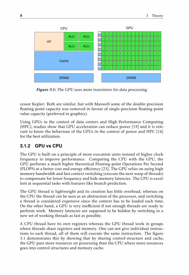
The Fast Fourier Transform is by far mostly associated with the Cooley-Tukey al-gorithm [7]. The Cooley-Tukey algorithm is a devide-and-conquer algorithm thatrecursively breaks down a DFT of any composite size of N = N1 ·N2. The algo-rithm decomposes the DFT into s = logr N stages. The N -point DFT is composedof r-point small DFTs in s stages. In this context the r-point DFT is called radix-rbutterfly.

Butterfly and radix-2

The implementation of anN -point radix-2 FFT algorithm have log2 N stages withN/2 butterfly operations per stage. A butterfly operation is an addition, and asubtraction, followed by a multiplication by a twiddle factor, see figure 3.2.

Figure 3.3 shows an 8-point radix-2 Decimation-In-Frequency (DIF) FFT. Theinput data are in natural order whereas the output data are in bit-reversed order.

10 3 Theory

x(0)

x(1)

x(2)

x(3)

x(4)

x(5)

x(6)

x(7)

X(0)

X(4)

X(2)

X(6)

X(1)

X(5)

X(3)

X(7)

×

×

×

×

×

×

×

×

W0N

W1N

W2N

W3N

W0N

W0N

W2N

W2N

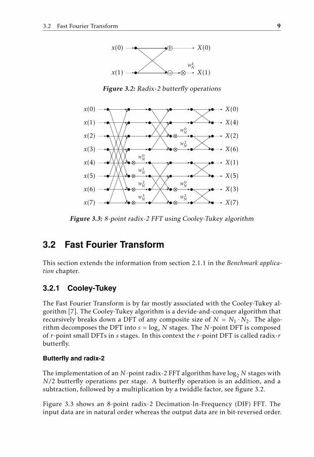
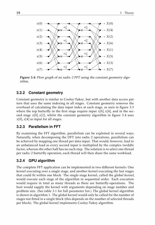
Figure 3.4: Flow graph of an radix-2 FFT using the constant geometry algo-rithm.

3.2.2 Constant geometry

Constant geometry is similar to Cooley-Tukey, but with another data access pat-tern that uses the same indexing in all stages. Constant geometry removes theoverhead of calculating the data input index at each stage, as seen in figure 3.3where the top butterfly in the first stage require input x[0], x[4], and in the sec-ond stage x[0], x[2], whilst the constant geometry algorithm in figure 3.4 usesx[0], x[4] as input for all stages.

3.2.3 Parallelism in FFT

By examining the FFT algorithm, parallelism can be exploited in several ways.Naturally, when decomposing the DFT into radix-2 operations, parallelism canbe achieved by mapping one thread per data input. That would, however, lead toan unbalanced load as every second input is multiplied by the complex twiddlefactor, whereas the other half has no such step. The solution is to select one threadper radix-2 butterfly operation, each thread will then share the same workload.

3.2.4 GPU algorithm

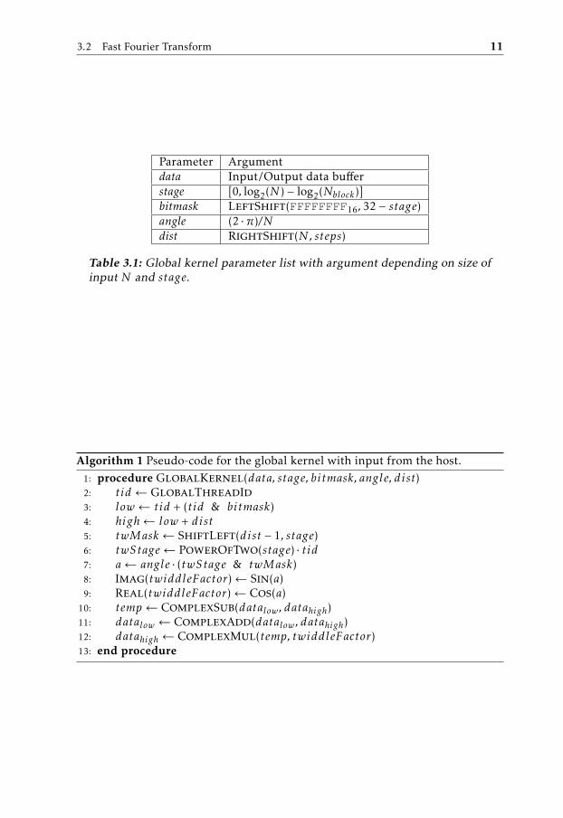
The complete FFT application can be implemented in two different kernels: Onekernel executing over a single stage, and another kernel executing the last stagesthat could fit within one block. The single-stage kernel, called the global kernel,would execute each stage of the algorithm in sequential order. Each executionwould require in total as many threads as there are butterfly-operations. Thehost would supply the kernel with arguments depending on stage number andproblem size. (See table 3.1 for full parameter list.) The global kernel algorithmis shown in algorithm 1. The global kernel would only be called for the number ofstages not fitted in a single block (this depends on the number of selected threadsper block). The global kernel implements Cooley-Tukey algorithm.

3.2 Fast Fourier Transform 11

Parameter Argumentdata Input/Output data bufferstage [0, log2(N ) − log2(Nblock)]bitmask LeftShift(FFFFFFFF16, 32 − stage)angle (2 ·π)/Ndist RightShift(N, steps)

Table 3.1: Global kernel parameter list with argument depending on size ofinput N and stage.

Algorithm 1 Pseudo-code for the global kernel with input from the host.1: procedure GlobalKernel(data, stage, bitmask, angle, dist)2: tid ← GlobalThreadId3: low← tid + (tid & bitmask)4: high← low + dist5: twMask ← ShiftLeft(dist − 1, stage)6: twStage← PowerOfTwo(stage) · tid7: a← angle · (twStage & twMask)8: Imag(twiddleFactor)← Sin(a)9: Real(twiddleFactor)← Cos(a)

10: temp← ComplexSub(datalow, datahigh)11: datalow ← ComplexAdd(datalow, datahigh)12: datahigh ← ComplexMul(temp, twiddleFactor)13: end procedure

12 3 Theory

Parameter Argumentin Input data bufferout Output data bufferangle (2 ·π)/Nstages [log2(N ) − log2(Nblock), log2(N )]leadingBits 32 − log2(N )c Forward: −1, Inverse: 1/N

Table 3.2: Local kernel parameter list with argument depending on size ofinput N and number of stages left to complete.

Shared/Local memory

The local kernel is always called, and encapsulates all remaining stages and thebit-reverse order output procedure. It is devised as to utilize shared memorycompletely for all stages. This reduces the primary memory accesses to a singleread and write per data point. The kernel implements the constant geometryalgorithm to increase performance in the inner loop: the input and output indexis only calculated once. See algorithm 2.

Register width

The targeted GPUs work on 32 bit registers and all fast integer arithmetic is basedon that. Procedures using bitwise operations are constructed with this architec-tural specific information, as seen in the bitmask parameter in table 3.1 and theleadingBits parameter in table 3.2. The bitmask parameter is used to get the off-set for each stage using the Cooley-Tukey algorithm. The leadingBits parameteris used in the bit-reverse operation to remove the leading zeroes that comes as aresult of the use of a 32 bit register.

Bit-reverse example: If the total size is 1024 elements, the last log2(1024) = 10bits are used. When encountering 1008 = 11111100002 for bit-reversal in thiscontext (with a problem size of 1024 points) the result is 63. However, using a 32bit register:

1008 = 000000000000000000000011111100002 (3.1)

bits reversed:

264241152 = 000011111100000000000000000000002 (3.2)

The leading zeroes becomes trailing zeroes that needs to be removed. A logicright shift operation by the length of leadingBits = 32 − log2(1024) = 22 solvesthis.

3.3 Related research

Scientific interest have mainly been targeting CUDA and OpenCL for compar-isons. Benchmarking between the two have established that there is difference

3.3 Related research 13

Algorithm 2 Pseudo-code for the local kernel with input from the host.1: procedure LocalKernel(in, out, angle, stages, leadingBits, c)2: let shared be a shared/local memory buffer3: low← ThreadId4: high← low + BlockDim5: of f set ← BlockId ·BlockDim · 26: sharedlow ← inlow+of f set7: sharedhigh ← inhigh+of f set8: ConstantGeometry(shared, low, high, angle, stages)9: revLow← BitReverse(low + of f set, leadingBits)

10: revHigh← BitReverse(high + of f set, leadingBits)11: outrevLow ← ComplexMul(c, sharedlow)12: outrevHigh ← ComplexMul(c, sharedhigh)13: end procedure

14: procedure ConstantGeometry(shared, low, high, angle, stages)15: outi ← low · 216: outii ← outI + 117: for stage← 0, stages − 1 do18: bitmask ← ShiftLeft(0xFFFFFFFF, stage)19: a← angle · (low & bitmask)20: Imag(twiddleFactor)← Sin(a)21: Real(twiddleFactor)← Cos(a)22: temp← ComplexSub(sharedlow, sharedhigh)23: sharedouti ← ComplexAdd(sharedlow, sharedhigh)24: sharedoutii ← ComplexMul(twiddleFactor, temp)25: end for26: end procedure

14 3 Theory

in favour of CUDA, however it can be due to unfair comparisons [10], and withthe correct tuning OpenCL can be just as fast. The same paper stated that thebiggest difference came from running the forward FFT algorithm. Examinationshowed that large differences could be found in the Parallel Thread Execution(PTX) instructions (intermediary GPU code).

Porting from CUDA to OpenCL without loosing performance have been exploredin [9], where the goal was to achieve a performance-portable solution. Some ofthe main differences between the technologies are described in that paper.

4Technologies

Five different multi-core technologies are used in this study. One is a proprietaryparallel computing platform and API, called CUDA. Compute Shaders in OpenGLand DirectCompute are parts of graphic programming languages but have a fairlygeneral structure and allows for general computing. OpenCL have a stated goalto target any heterogeneous multi-core system but is used in this study solely onthe GPU. To compare with the CPU, OpenMP is included as an effective way toparallelize sequential C/C++-code.

4.1 CUDA

CUDA is developed by NVIDIA and was released in 2006. CUDA is an extensionof the C/C++ language and have its own compiler. CUDA supports the function-ality to execute kernels, and modify the graphic card RAM memory and the useof several optimized function libraries such as cuBLAS (CUDA implementationof Basic Linear Algebra Subprograms (BLAS)) and cuFFT (CUDA implementationof FFT).

A program launched on the GPU is called a kernel. The GPU is referred to asthe device and the the CPU is called the host. To run a CUDA kernel, all that isneeded is to declare the program with the function type specifier __global__and call it from the host with launch arguments, for other specifiers see table 4.1.The kernel execution call includes specifying the thread organization. Threadsare organized in blocks, that in turn are specified within a grid. Both the blockand grid can be used as One-dimensional (1D), Two-dimensional (2D) or Three-dimensional (3D) to help the addressing in a program. These can be accessedwithin a kernel by the structures blockDim and gridDim. Thread and block

15

16 4 Technologies

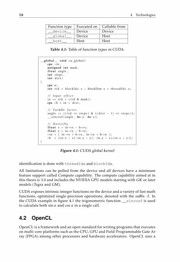
Function type Executed on Callable from__device__ Device Device__global__ Device Host__host__ Host Host

Table 4.1: Table of function types in CUDA.

__global__ void cu_global (cpx * in ,unsigned int mask ,f l oa t angle ,int steps ,int d i s t )

{cpx w;int t i d = blockIdx . x * blockDim . x + threadIdx . x ;

/ / Input o f f s e tin += t i d + ( t i d & mask ) ;cpx *h = in + d i s t ;

/ / Twiddle f a c t o rangle *= ( ( t i d << steps ) & ( ( d i s t − 1) << steps ) ) ;_ _ s i n c o s f ( angle , &w. y , &w. x ) ;

/ / B u t t e r f l yf l oa t x = in−>x − h−>x ;f l oa t y = in−>y − h−>y ;* in = { in−>x + h−>x , in−>y + h−>y } ;*h = { (w. x * x ) − (w. y * y ) , (w. y * x )+(w. x * y ) } ;

}

Figure 4.1: CUDA global kernel

identification is done with threadIdx and blockIdx.

All limitations can be polled from the device and all devices have a minimumfeature support called Compute capability. The compute capability aimed at inthis thesis is 3.0 and includes the NVIDIA GPU models starting with GK or latermodels (Tegra and GM ).

CUDA exposes intrinsic integer functions on the device and a variety of fast mathfunctions, optimized single-precision operations, denoted with the suffix -f. Inthe CUDA example in figure 4.1 the trigonometric function __sincosf is usedto calculate both sinα and cosα in a single call.

4.2 OpenCL

OpenCL is a framework and an open standard for writing programs that executeson multi-core platforms such as the CPU, GPU and Field-Programmable Gate Ar-ray (FPGA) among other processors and hardware accelerators. OpenCL uses a

4.2 OpenCL 17

__kernel void o c l _ g l o b a l (__global cpx * in ,f l oa t angle ,unsigned int mask ,int steps ,int d i s t )

{cpx w;int t i d = get_g loba l_ id ( 0 ) ;

/ / Input o f f s e tin += t i d + ( t i d & mask ) ;cpx *high = in + d i s t ;

/ / Twiddle f a c t o rangle *= ( ( t i d << steps ) & ( ( d i s t − 1) << steps ) ) ;w. y = s i n c o s ( angle , &w. x ) ;

/ / B u t t e r f l yf l oa t x = in−>x − high−>x ;f l oa t y = in−>y − high−>y ;in−>x = in−>x + high−>x ;in−>y = in−>y + high−>y ;high−>x = (w. x * x ) − (w. y * y ) ;high−>y = (w. y * x ) + (w. x * y ) ;

}

Figure 4.2: OpenCL global kernel

similar structure as CUDA: The language is based on C99 when programming adevice. The standard is supplied by the The Khronos Groups and the implemen-tation is supplied by the manufacturing company or device vendor such as AMD,INTEL, or NVIDIA.

OpenCL views the system from a perspective where computing resources (CPUor other accelerators) are a number of compute devices attached to a host (a CPU).The programs executed on a compute device is called a kernel. Programs in theOpenCL language are intended to be compiled at run-time to preserve portabilitybetween implementations from various host devices.

The OpenCL kernels are compiled by the host and then enqueued on a computedevice. The kernel function accessible by the host to enqueue is specified with__kernel. Data residing in global memory is specified in the parameter list by__global and local memory have the specifier __local. The CUDA threadsare in OpenCL terminology called Work-items and they are organized in Work-groups.

Similarly to CUDA the host application can poll the device for its capabilities anduse some fast math function. The equivalent CUDA kernel in figure 4.1 is imple-mented in OpenCL in figure 4.2 and displays small differences. The OpenCLmath function sincos is the equivalent of __sincosf.

18 4 Technologies

[ numthreads (GROUP_SIZE_X , 1 , 1 ) ]void dx_global (

uint3 threadIDInGroup : SV_GroupThreadID ,uint3 groupID : SV_GroupID ,uint groupIndex : SV_GroupIndex ,uint3 dispatchThreadID : SV_DispatchThreadID )

{cpx w;int t i d = groupID . x * GROUP_SIZE_X + threadIDInGroup . x ;

/ / Input o f f s e tint in_low = t i d + ( t i d & mask ) ;int in_high = in_low + d i s t ;

/ / Twiddle f a c t o rf l oa t a = angle * ( ( t id <<steps )& ( ( d i s t − 1)<< steps ) ) ;s i n c o s ( a , w. y , w. x ) ;

/ / B u t t e r f l yf l oa t x = input [ in_low ] . x − input [ in_high ] . x ;f l oa t y = input [ in_low ] . y − input [ in_high ] . y ;rw_buf [ in_low ] . x = input [ in_low ] . x + input [ in_high ] . x ;rw_buf [ in_low ] . y = input [ in_low ] . y + input [ in_high ] . y ;rw_buf [ in_high ] . x = (w. x * x ) − (w. y * y ) ;rw_buf [ in_high ] . y = (w. y * x ) + (w. x * y ) ;

}

Figure 4.3: DirectCompute global kernel

4.3 DirectCompute

Microsoft DirectCompute is an API that supports GPGPU on Microsoft’s Win-dows Operating System (OS) (Vista, 7, 8, 10). DirectCompute is part of the Di-rectX collection of APIs. DirectX was created to support computer games devel-opment for the Windows 95 OS. The initial release of DirectCompute was withDirectX 11 API, and have similarities with both CUDA and OpenCL. DirectCom-pute is designed and implemented with HLSL. The program (and kernel equiva-lent) is called a compute shader. The compute shader is not like the other typesof shaders that are used in the graphic processing pipeline (like vertex or pixelshaders).

A difference from CUDA and OpenCL in implementing a compute shader com-pared to a kernel is the lack of C-like parameters: A constant buffer is used in-stead, where each value is stored in a read-only data structure. The setup sharesimilarities with OpenCL and the program is compiled at run-time. The threaddimensions is built in as a constant value in the compute shader, and the blockdimensions are specified at shader dispatch/execution.

As the code example demonstrated in figure 4.3 the shader body is similar to thatof CUDA and OpenCL.

4.4 OpenGL 19

void main ( ){

cpx w;uint t i d = gl_GlobalInvocat ionID . x ;

/ / Input o f f s e tuint in_low = t i d + ( t i d & mask ) ;uint in_high = in_low + d i s t ;

/ / Twiddle f a c t o rf l oa t a = angle * ( ( t id <<steps )& ( ( d i s t − 1U)<< steps ) ) ;w. x = cos ( a ) ;w. y = s in ( a ) ;

/ / B u t t e r f l ycpx low = data [ in_low ] ;cpx high = data [ in_high ] ;f l oa t x = low . x − high . x ;f l oa t y = low . y − high . y ;data [ in_low ] = cpx ( low . x + high . x , low . y + high . y ) ;data [ in_high ] = cpx ( (w. x *x ) − (w. y*y ) , (w. y*x )+(w. x *y ) ) ;

}

Figure 4.4: OpenGL global kernel

4.4 OpenGL

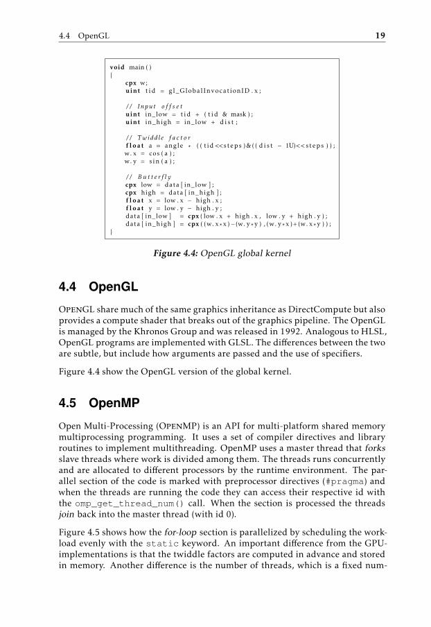
OpenGL share much of the same graphics inheritance as DirectCompute but alsoprovides a compute shader that breaks out of the graphics pipeline. The OpenGLis managed by the Khronos Group and was released in 1992. Analogous to HLSL,OpenGL programs are implemented with GLSL. The differences between the twoare subtle, but include how arguments are passed and the use of specifiers.

Figure 4.4 show the OpenGL version of the global kernel.

4.5 OpenMP

Open Multi-Processing (OpenMP) is an API for multi-platform shared memorymultiprocessing programming. It uses a set of compiler directives and libraryroutines to implement multithreading. OpenMP uses a master thread that forksslave threads where work is divided among them. The threads runs concurrentlyand are allocated to different processors by the runtime environment. The par-allel section of the code is marked with preprocessor directives (#pragma) andwhen the threads are running the code they can access their respective id withthe omp_get_thread_num() call. When the section is processed the threadsjoin back into the master thread (with id 0).

Figure 4.5 shows how the for-loop section is parallelized by scheduling the work-load evenly with the static keyword. An important difference from the GPU-implementations is that the twiddle factors are computed in advance and storedin memory. Another difference is the number of threads, which is a fixed num-

20 4 Technologies

void add_sub_mul ( cpx * l , cpx *u , cpx *out , cpx *w){

f l oa t x = l−>x − u−>x ;f l oa t y = l−>y − u−>y ;* out = { l−>x + u−>x , l−>y + u−>y } ;*(++ out ) = { (w−>x *x ) − (w−>y*y ) , (w−>y*x )+(w−>x *y ) } ;

}void f f t _ s t a g e ( cpx * i , cpx *o , cpx *w, uint m, int r ){#pragma omp p a r a l l e l for schedule ( s t a t i c )

for ( int l = 0 ; l < r ; ++l )add_sub_mul ( i +l , i +r+l , o+( l <<1) ,w+( l & m) ) ;

}

Figure 4.5: OpenMP procedure completing one stage

ber where each thread will work on a consecutive span of the iterated butterflyoperations.

4.6 External libraries

External libraries were selected for reference values. FFTW and cuFFT were se-lected because they are frequently used in other papers. clFFT was selected bythe assumption that it is the AMD equivalent of cuFFT for AMDs graphic cards.

FFTW

Fastest Fourier Transform in the West (FFTW) is a C subroutine library for com-puting the DFT. FFTW is a free software[11] that have been available since 1997,and several papers have been published about the FFTW [12, 13, 14]. FFTW sup-ports a variety of algorithms and by estimating performance it builds a plan toexecute the transform. The estimation can be done by either performance test ofan extensive set of algorithms, or by a few known fast algorithms.

cuFFT

The library cuFFT (NVIDIA CUDA Fast Fourier Transform product) [21] is de-signed to provide high-performance on NVIDIA GPUs. cuFFT uses algorithmsbased on the Cooley-Tukey and the Bluestein algorithm [4].

clFFT

The library clFFT, found in [3] is part of the open source AMD Compute Libraries(ACL)[2]. According to an AMD blog post[1] the library performs at a similarlevel of cuFFT1.

1The performance tests was done using NVIDIA Tesla K40 for cuFFT and AMD Firepro W9100for clFFT.

5Implementation

The FFT application has been implemented in C/C++, CUDA, OpenCL, Direct-Compute, and OpenGL. The application was tested on a GeForce GTX 670 and aRadeon R7 R260X graphics card and on an Intel Core i7 3770K 3.5GHz CPU.

5.1 Benchmark application GPU

5.1.1 FFT

Setup

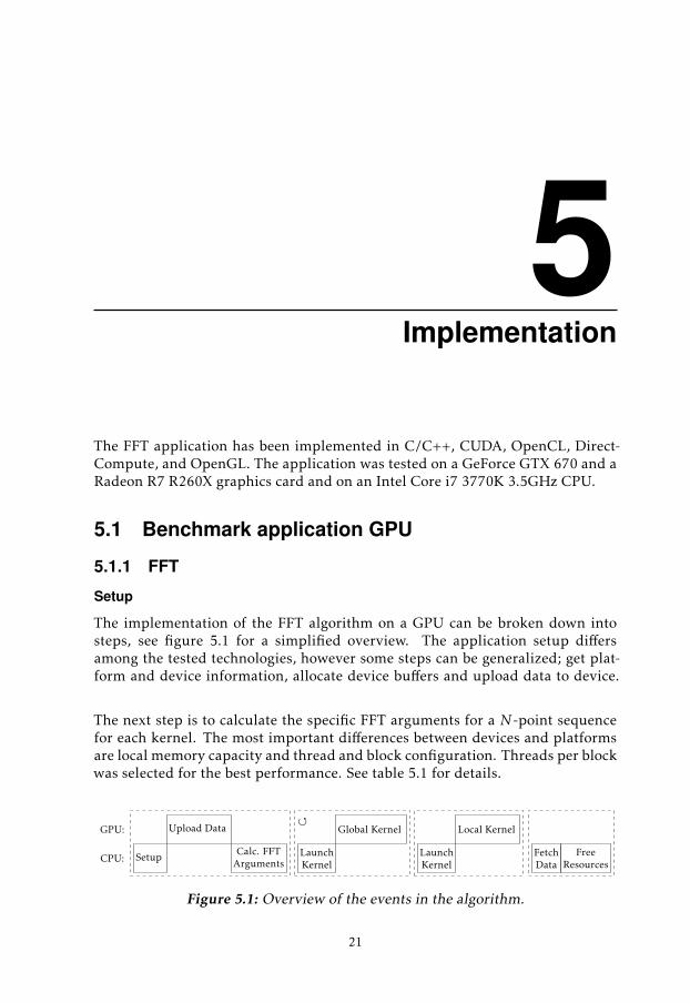
The implementation of the FFT algorithm on a GPU can be broken down intosteps, see figure 5.1 for a simplified overview. The application setup differsamong the tested technologies, however some steps can be generalized; get plat-form and device information, allocate device buffers and upload data to device.

The next step is to calculate the specific FFT arguments for a N -point sequencefor each kernel. The most important differences between devices and platformsare local memory capacity and thread and block configuration. Threads per blockwas selected for the best performance. See table 5.1 for details.

Setup

Upload Data

Calc. FFTArgumentsCPU:

GPU:

LaunchKernel

Global Kernel

LaunchKernel

Local Kernel

FetchData

FreeResources

Figure 5.1: Overview of the events in the algorithm.

21

22 5 Implementation

Device Technology Threads / Block Max Threads Shared memory

GeForce GTX 670

CUDA 1024

1024

49152OpenCL 512 49152OpenGL 1024 32768DirectX 1024 32768

Radeon R7 260XOpenCL 256

256 32768OpenGL 256DirectX 256

Table 5.1: Shared memory size in bytes, threads and block configuration perdevice.

Thread and block scheme

The threading scheme was one butterfly per thread, so that a sequence of six-teen points require eight threads. Each platform was configured to a number ofthreads per block (see table 5.1): any sequences requiring more butterfly oper-ations than the threads per block configuration needed the computations to besplit over several blocks. In the case of a sequence exceeding one block, the se-quence is mapped over the blockIdx.y dimension with size gridDim.y. Theblock dimensions are limited to 231, 216, 216 respectively for x, y, z. Example: ifthe threads per block limit is two, then four blocks would be needed for a sixteenpoint sequence.

Synchronization

Thread synchronization is only available of threads within a block. When thesequence or partial sequence fitted within a block, that part was transferred tolocal memory before computing the last stages. If the sequence was larger andrequired more than one block, the synchronization was handled by launching sev-eral kernels in the same stream to be executed in sequence. The kernel launchedfor block wide synchronization is called the global kernel and the kernel forthread synchronization within a block is called the local kernel. The global kernelhad an implementation of the Cooley-Tukey FFT algorithm, and the local kernelhad constant geometry (same indexing for every stage). The last stage outputsdata from the shared memory in bit-reversed order to the global memory. Seefigure 5.2, where the sequence length is 16 and the threads per block is set totwo.

Calculation

The indexing for the global kernel was calculated from the thread id and blockid (threadIdx.x and blockIdx.x in CUDA) as seen in figure 5.3. Input andoutput is located by the same index.

Index calculation for the local kernel is done once for all stages, see figure 5.4.These indexes are separate from the indexing in the global memory. The globalmemory offset depends on threads per block (blockDim.x in CUDA) and blockid.

5.1 Benchmark application GPU 23

x(0)

x(1)

x(2)

x(3)

x(4)

x(5)

x(6)

x(7)

x(8)

x(9)

x(10)

x(11)

x(12)

x(13)

x(14)

x(15)

X(0)

X(1)

X(2)

X(3)

X(4)

X(5)

X(6)

X(7)

X(8)

X(9)

X(10)

X(11)

X(12)

X(13)

X(14)

X(15)

××××××××

××××

××××

×

×

×

×

×

×

×

×

W016

W116

W216

W316

W416

W516

W616

W716

W08

W18

W28

W38

W08

W18

W28

W38

W04

W14

W04

W14

W04

W14

W04

W14

stage 1 stage 2 stage 3 stage 4 output

Figure 5.2: Flow graph of a 16-point FFT using (stage 1 and 2) Cooley-Tukeyalgorithm and (stage 3 and 4) constant geometry algorithm. The solid boxis the bit-reverse order output. Dotted boxes are separate kernel launches,dashed boxes are data transfered to local memory before computing the re-maining stages.

int t i d = blockIdx . x * blockDim . x + threadIdx . x ,io_low = t i d + ( t i d & (0 xFFFFFFFF << s t a g e s _ l e f t ) ) ,io_high = io_low + (N >> 1 ) ;

Figure 5.3: CUDA example code showing index calculation for each stage inthe global kernel, N is the total number of points. io_low is the index of thefirst input in the butterfly operation and io_high the index of the second.

24 5 Implementation

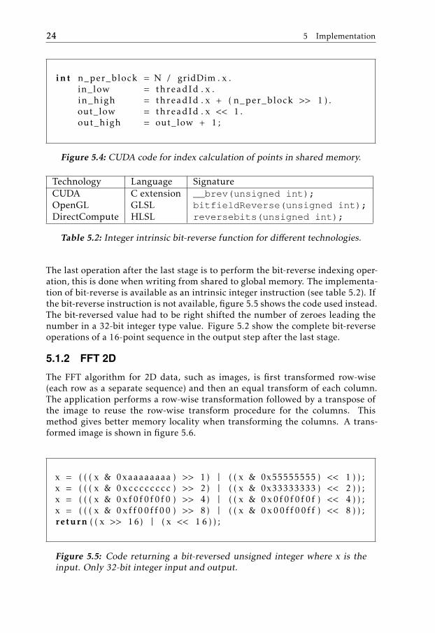
int n_per_block = N / gridDim . x .in_low = threadId . x .in_high = threadId . x + ( n_per_block >> 1 ) .out_low = threadId . x << 1 .out_high = out_low + 1 ;

Figure 5.4: CUDA code for index calculation of points in shared memory.

Technology Language SignatureCUDA C extension __brev(unsigned int);OpenGL GLSL bitfieldReverse(unsigned int);DirectCompute HLSL reversebits(unsigned int);

Table 5.2: Integer intrinsic bit-reverse function for different technologies.

The last operation after the last stage is to perform the bit-reverse indexing oper-ation, this is done when writing from shared to global memory. The implementa-tion of bit-reverse is available as an intrinsic integer instruction (see table 5.2). Ifthe bit-reverse instruction is not available, figure 5.5 shows the code used instead.The bit-reversed value had to be right shifted the number of zeroes leading thenumber in a 32-bit integer type value. Figure 5.2 show the complete bit-reverseoperations of a 16-point sequence in the output step after the last stage.

5.1.2 FFT 2D

The FFT algorithm for 2D data, such as images, is first transformed row-wise(each row as a separate sequence) and then an equal transform of each column.The application performs a row-wise transformation followed by a transpose ofthe image to reuse the row-wise transform procedure for the columns. Thismethod gives better memory locality when transforming the columns. A trans-formed image is shown in figure 5.6.

x = ( ( ( x & 0xaaaaaaaa ) >> 1) | ( ( x & 0x55555555 ) << 1 ) ) ;x = ( ( ( x & 0 xcccccccc ) >> 2) | ( ( x & 0x33333333 ) << 2 ) ) ;x = ( ( ( x & 0 xf0f0 f0 f0 ) >> 4) | ( ( x & 0 x0f0f0 f0 f ) << 4 ) ) ;x = ( ( ( x & 0 xf f00f f00 ) >> 8) | ( ( x & 0 x00f f00f f ) << 8 ) ) ;return ( ( x >> 16) | ( x << 1 6 ) ) ;

Figure 5.5: Code returning a bit-reversed unsigned integer where x is theinput. Only 32-bit integer input and output.

5.1 Benchmark application GPU 25

(a) Original image (b) Magnitude representation

Figure 5.6: Original image in 5.6a transformed and represented with a quad-rant shifted magnitude visualization (scale skewed for improved illustra-tion) in 5.6b.

The difference between the FFT kernel for 1D and 2D is the indexing scheme. 2Drows are indexed with blockIdx.x, and columns with threadIdx.x addedwith an offset of blockIdx.y · blockDim.x.

Transpose

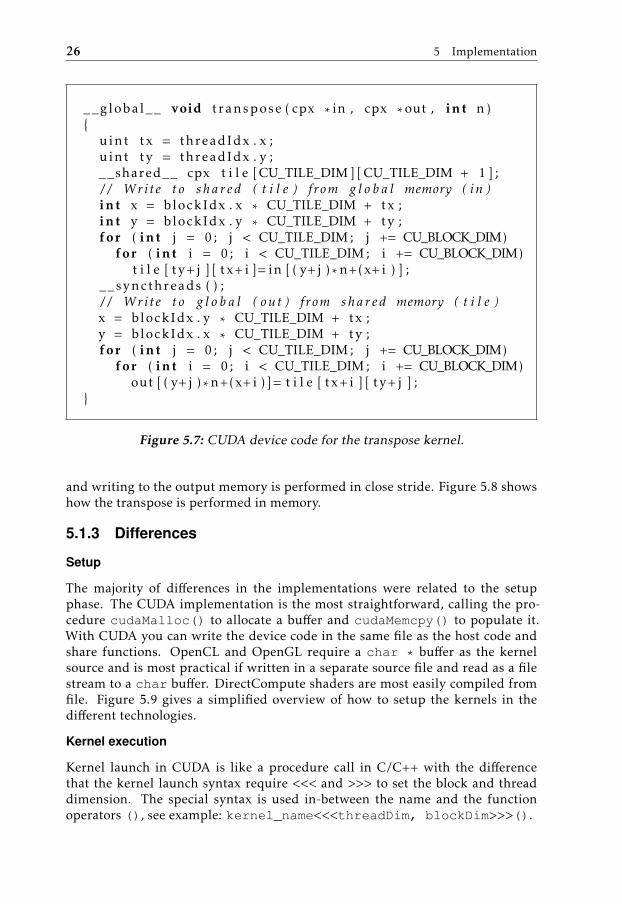
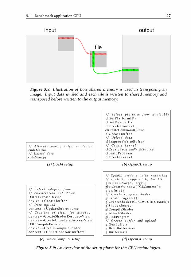
The transpose kernel uses a different index mapping of the 2D-data and threadsper blocks than the FFT kernel. The data is tiled in a grid pattern where each tilerepresents one block, indexed by blockIdx.x and blockIdx.y. The tile size isa multiple of 32 for both dimensions and limited to the size of the shared memorybuffer, see table 5.1 for specific size per technology. To avoid the banking issues,the last dimension is increased with one but not used. However, resolving thebanking issue have little effect on total running-time so when shared memoryis limited to 32768, the extra column is not used. The tile rows and columnsare divided over the threadIdx.x and threadIdx.y index respectively. Seefigure 5.7 for a code example of the transpose kernel.

Shared memory example: The CUDA shared memory can allocate 49152 bytesand a single data point require sizeof(float) · 2 = 8 bytes. That leaves roomfor a tile size of 64 · (64 + 1) · 8 = 33280 bytes. Where the integer 64 is the highestpower of two that fits.

The transpose kernel uses the shared memory and tiling of the image to avoidlarge strides through global memory. Each block represents a tile in the image.The first step is to write the complete tile to shared memory and synchronize thethreads before writing to the output buffer. Both reading from the input memory

26 5 Implementation

__global__ void transpose ( cpx * in , cpx *out , int n ){

uint tx = threadIdx . x ;uint ty = threadIdx . y ;__shared__ cpx t i l e [CU_TILE_DIM ] [ CU_TILE_DIM + 1 ] ;/ / Write t o shared ( t i l e ) from g l o b a l memory ( in )int x = blockIdx . x * CU_TILE_DIM + tx ;int y = blockIdx . y * CU_TILE_DIM + ty ;for ( int j = 0 ; j < CU_TILE_DIM ; j += CU_BLOCK_DIM)

for ( int i = 0 ; i < CU_TILE_DIM ; i += CU_BLOCK_DIM)t i l e [ ty+ j ] [ tx+ i ]= in [ ( y+ j ) *n+(x+ i ) ] ;

__syncthreads ( ) ;/ / Write t o g l o b a l ( out ) from shared memory ( t i l e )x = blockIdx . y * CU_TILE_DIM + tx ;y = blockIdx . x * CU_TILE_DIM + ty ;for ( int j = 0 ; j < CU_TILE_DIM ; j += CU_BLOCK_DIM)

for ( int i = 0 ; i < CU_TILE_DIM ; i += CU_BLOCK_DIM)out [ ( y+ j ) *n+(x+ i ) ]= t i l e [ tx+ i ] [ ty+ j ] ;

}

Figure 5.7: CUDA device code for the transpose kernel.

and writing to the output memory is performed in close stride. Figure 5.8 showshow the transpose is performed in memory.

5.1.3 Differences

Setup

The majority of differences in the implementations were related to the setupphase. The CUDA implementation is the most straightforward, calling the pro-cedure cudaMalloc() to allocate a buffer and cudaMemcpy() to populate it.With CUDA you can write the device code in the same file as the host code andshare functions. OpenCL and OpenGL require a char * buffer as the kernelsource and is most practical if written in a separate source file and read as a filestream to a char buffer. DirectCompute shaders are most easily compiled fromfile. Figure 5.9 gives a simplified overview of how to setup the kernels in thedifferent technologies.

Kernel execution

Kernel launch in CUDA is like a procedure call in C/C++ with the differencethat the kernel launch syntax require <<< and >>> to set the block and threaddimension. The special syntax is used in-between the name and the functionoperators (), see example: kernel_name<<<threadDim, blockDim>>>().

5.1 Benchmark application GPU 27

input

tile

output

Figure 5.8: Illustration of how shared memory is used in transposing animage. Input data is tiled and each tile is written to shared memory andtransposed before written to the output memory.

/ / A l l o c a t e memory b u f f e r on d e v i c ecudaMalloc/ / Upload datacudaMemcpy

(a) CUDA setup

/ / S e l e c t p l a t f o rm from a v a i l a b l eclGetPlatformIDsclGetDeviceIDsclCreateContextclCreateCommandQueuec lCrea teBuf fer/ / Upload dataclEnqueueWriteBuffer/ / Crea t e k e r n e lclCreateProgramWithSourceclBuildProgramclCreateKernel

(b) OpenCL setup

/ / S e l e c t adap t e r from/ / enumerat ion not shownD3D11CreateDevicedevice−>CreateBuffer/ / Data uploadcontext −>UpdateSubresource/ / Crea t i on o f v iews f o r a c c e s s .device−>CreateShaderResourceViewdevice−>CreateUnorderedAccessViewD3DCompileFromFiledevice−>CreateComputeShadercontext −>CSSetConstantBuffers

(c) DirectCompute setup

/ / OpenGL needs a v a l i d r ende r ing/ / con t ex t , s upp l i e d by the OS .g l u t I n i t (&argc , argv ) ;glutCreateWindow ( " GLContext " ) ;g lewIni t ( ) ;/ / Crea t e compute shaderglCreateProgram ( ) ;glCreateShader (GL_COMPUTE_SHADER ) ;glShaderSourceglCompileShaderglAttachShaderglLinkProgram/ / Crea t e b u f f e r and uploadglGenBuffersglBindBufferBaseglBufferData

(d) OpenGL setup

Figure 5.9: An overview of the setup phase for the GPU technologies.

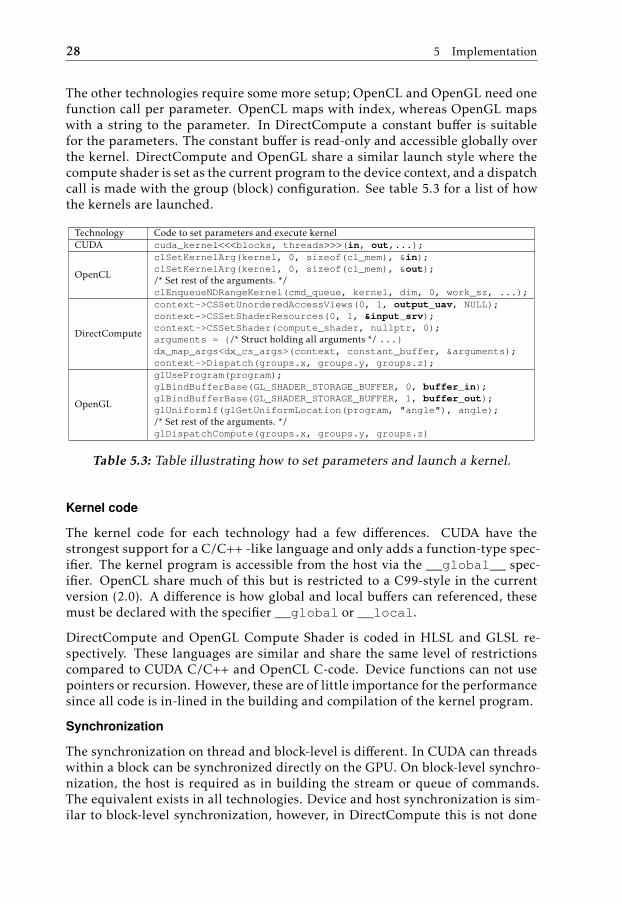
28 5 Implementation

The other technologies require some more setup; OpenCL and OpenGL need onefunction call per parameter. OpenCL maps with index, whereas OpenGL mapswith a string to the parameter. In DirectCompute a constant buffer is suitablefor the parameters. The constant buffer is read-only and accessible globally overthe kernel. DirectCompute and OpenGL share a similar launch style where thecompute shader is set as the current program to the device context, and a dispatchcall is made with the group (block) configuration. See table 5.3 for a list of howthe kernels are launched.

Technology Code to set parameters and execute kernelCUDA cuda_kernel<<<blocks, threads>>>(in, out,...);

OpenCL

clSetKernelArg(kernel, 0, sizeof(cl_mem), &in);clSetKernelArg(kernel, 0, sizeof(cl_mem), &out);/* Set rest of the arguments. */clEnqueueNDRangeKernel(cmd_queue, kernel, dim, 0, work_sz, ...);

DirectCompute

context->CSSetUnorderedAccessViews(0, 1, output_uav, NULL);context->CSSetShaderResources(0, 1, &input_srv);context->CSSetShader(compute_shader, nullptr, 0);arguments = {/* Struct holding all arguments */ ...}dx_map_args<dx_cs_args>(context, constant_buffer, &arguments);context->Dispatch(groups.x, groups.y, groups.z);

OpenGL

glUseProgram(program);glBindBufferBase(GL_SHADER_STORAGE_BUFFER, 0, buffer_in);glBindBufferBase(GL_SHADER_STORAGE_BUFFER, 1, buffer_out);glUniform1f(glGetUniformLocation(program, "angle"), angle);/* Set rest of the arguments. */glDispatchCompute(groups.x, groups.y, groups.z)

Table 5.3: Table illustrating how to set parameters and launch a kernel.

Kernel code

The kernel code for each technology had a few differences. CUDA have thestrongest support for a C/C++ -like language and only adds a function-type spec-ifier. The kernel program is accessible from the host via the __global__ spec-ifier. OpenCL share much of this but is restricted to a C99-style in the currentversion (2.0). A difference is how global and local buffers can referenced, thesemust be declared with the specifier __global or __local.

DirectCompute and OpenGL Compute Shader is coded in HLSL and GLSL re-spectively. These languages are similar and share the same level of restrictionscompared to CUDA C/C++ and OpenCL C-code. Device functions can not usepointers or recursion. However, these are of little importance for the performancesince all code is in-lined in the building and compilation of the kernel program.

Synchronization

The synchronization on thread and block-level is different. In CUDA can threadswithin a block can be synchronized directly on the GPU. On block-level synchro-nization, the host is required as in building the stream or queue of commands.The equivalent exists in all technologies. Device and host synchronization is sim-ilar to block-level synchronization, however, in DirectCompute this is not done

5.2 Benchmark application CPU 29

Setup TwiddleFactors

CalculateStage

BitReverseOrder

log2(N ) times

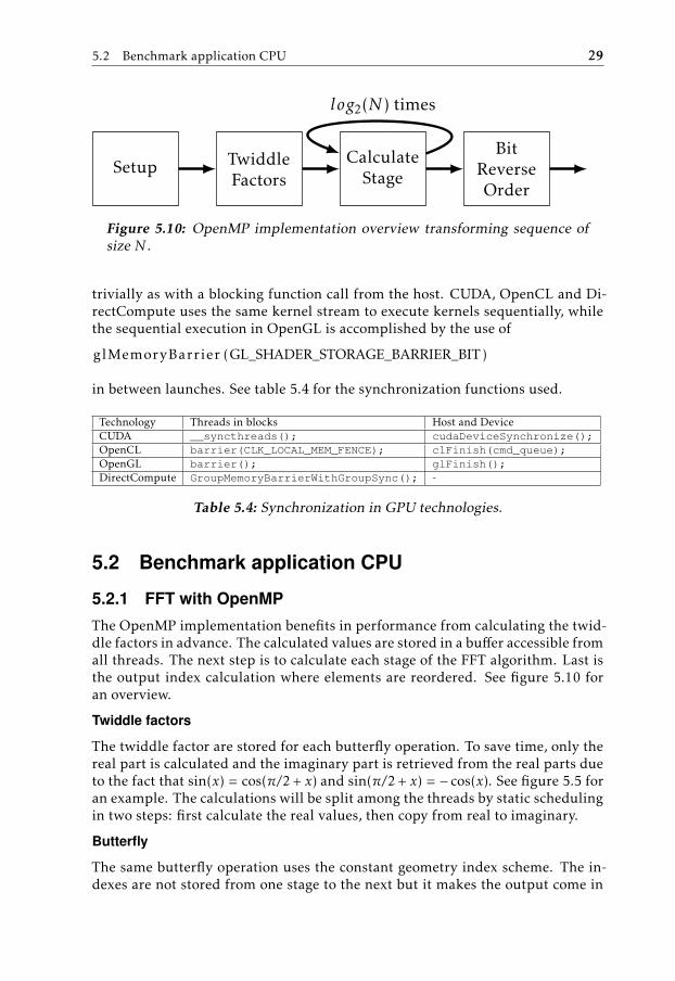
Figure 5.10: OpenMP implementation overview transforming sequence ofsize N .

trivially as with a blocking function call from the host. CUDA, OpenCL and Di-rectCompute uses the same kernel stream to execute kernels sequentially, whilethe sequential execution in OpenGL is accomplished by the use of

glMemoryBarrier (GL_SHADER_STORAGE_BARRIER_BIT)

in between launches. See table 5.4 for the synchronization functions used.

Technology Threads in blocks Host and DeviceCUDA __syncthreads(); cudaDeviceSynchronize();OpenCL barrier(CLK_LOCAL_MEM_FENCE); clFinish(cmd_queue);OpenGL barrier(); glFinish();DirectCompute GroupMemoryBarrierWithGroupSync(); -

Table 5.4: Synchronization in GPU technologies.

5.2 Benchmark application CPU

5.2.1 FFT with OpenMP

The OpenMP implementation benefits in performance from calculating the twid-dle factors in advance. The calculated values are stored in a buffer accessible fromall threads. The next step is to calculate each stage of the FFT algorithm. Last isthe output index calculation where elements are reordered. See figure 5.10 foran overview.

Twiddle factors

The twiddle factor are stored for each butterfly operation. To save time, only thereal part is calculated and the imaginary part is retrieved from the real parts dueto the fact that sin(x) = cos(π/2 + x) and sin(π/2 + x) = − cos(x). See figure 5.5 foran example. The calculations will be split among the threads by static schedulingin two steps: first calculate the real values, then copy from real to imaginary.

Butterfly

The same butterfly operation uses the constant geometry index scheme. The in-dexes are not stored from one stage to the next but it makes the output come in

30 5 Implementation

Twiddle factor table Wi <(W ) =(W )0 cos(α · 0) <(W [4])1 cos(α · 1) <(W [5])2 cos(α · 2) <(W [6])3 cos(α · 3) <(W [7])4 cos(α · 4) −<(W [0])5 cos(α · 5) −<(W [1])6 cos(α · 6) −<(W [2])7 cos(α · 7) −<(W [3])

Table 5.5: Twiddle factors for a 16-point sequence where α equals (2 ·π)/16.Each row i corresponds to the ith butterfly operation.

void omp_bit_reverse ( cpx *x , int l ead ing_bi t s , int N){#pragma omp p a r a l l e l for schedule ( s t a t i c )

for ( int i = 0 ; i <= N; ++ i ) {int p = b i t _ r e v e r s e ( i , l e a d i n g _ b i t s ) ;i f ( i < p )

swap(&( x [ i ] ) , &(x [ p ] ) ) ;}

}

Figure 5.11: C/C++ code performing the bit-reverse ordering of a N-pointsequence.

continuous order. The butterfly operations are split among the threads by staticscheduling.

Bit-Reversed Order

See figure 5.11 for code showing the bit-reverse ordering operation in C/C++code.

5.2.2 FFT 2D with OpenMP

The implementation of 2D FFT with OpenMP runs the transformations row-wiseand transposes the image and repeat. The twiddle factors are calculated once andstays the same.

5.2.3 Differences with GPU

The OpenMP implementation is different from the GPU-implementations in twoways: twiddle factors are pre-computed, and all stages uses the constant geom-

5.3 Benchmark configurations 31

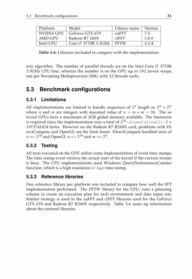
Platform Model Library name VersionNVIDIA GPU GeForce GTX 670 cuFFT 7.5AMD GPU Radeon R7 260X clFFT 2.8.0Intel CPU Core i7 3770K 3.5GHz FFTW 3.3.4

Table 5.6: Libraries included to compare with the implementation.

etry algorithm. The number of parallel threads are on the Intel Core i7 3770K3.5GHz CPU four, whereas the number is on the GPU up to 192 (seven warps,one per Streaming Multiprocessor (SM), with 32 threads each).

5.3 Benchmark configurations

5.3.1 Limitations

All implementations are limited to handle sequences of 2n length or 2m × 2m

where n and m are integers with maximal value of n = m + m = 26. The se-lected GPUs have a maximum of 2GB global memory available. The limitationis required since the implementation uses a total of 226 ·sizeof(float2) · 2 =1073741824 bytes. However on the Radeon R7 R260X card, problems with Di-rectCompute and OpenGL set the limit lower. DirectCompute handled sizes ofn <= 224 and OpenGL n <= 224 and m <= 29.

5.3.2 Testing

All tests executed on the GPU utilize some implementation of event time stamps.The time stamp event retrieve the actual start of the kernel if the current streamis busy. The CPU implementations used Windows QueryPerformanceCounterfunction, which is a high resolution (< 1µs) time stamp.

5.3.3 Reference libraries

One reference library per platform was included to compare how well the FFTimplementation performed. The FFTW library for the CPU, runs a planningscheme to create an execution plan for each environment and data input size.Similar strategy is used in the cuFFT and clFFT libraries used for the GeForceGTX 670 and Radeon R7 R260X respectively. Table 5.6 sums up informationabout the external libraries.

6Evaluation

6.1 Results

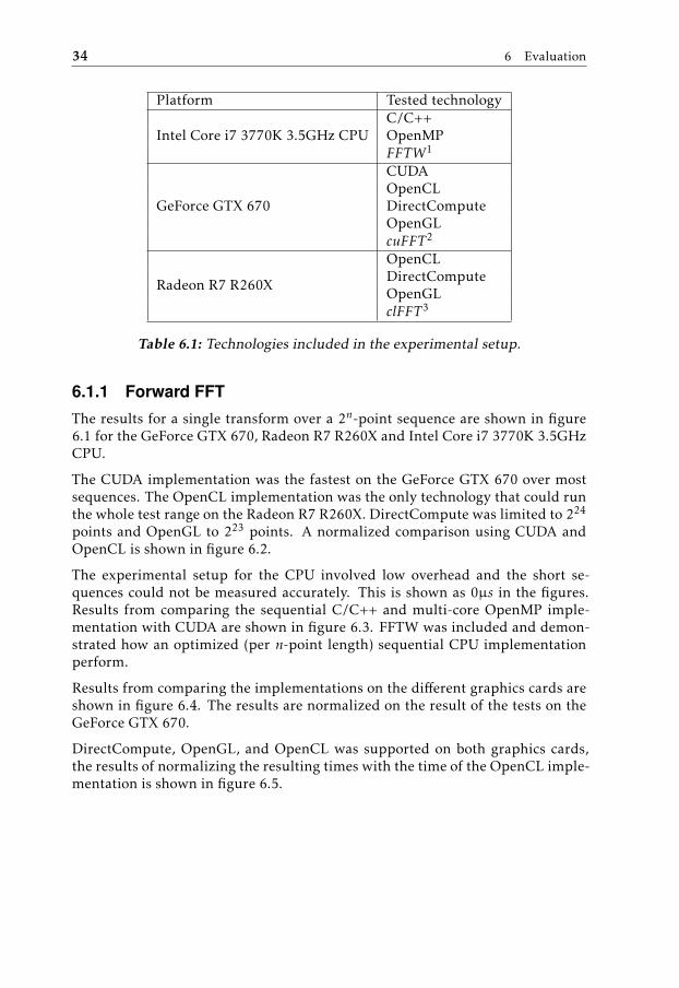
The results will be shown for the two graphics cards GeForce GTX 670 andRadeon R7 R260X, where the technologies were applicable. The tested technolo-gies are shown in table 6.1. The basics of each technology or library is explainedin chapter 4.

The performance measure is total execution time for a single forward transformusing two buffers: one input and one output buffer. The implementation inputsize range is limited by the hardware (graphics card primary memory). Howeverthere are some unsolved issues near the upper limit on some technologies on theRadeon R7 R260X.

CUDA is the primary technology and the GeForce GTX 670 graphics card is theprimary platform. All other implementations are ported from CUDA implemen-tation. To compare the implementation, external libraries are included and canbe found in italics in the table 6.1. Note that the clFFT library failed to be mea-sured in the same manner as the other GPU implementations: the times are mea-sured at host, and short sequences suffer from large overhead.

The experiments are tuned on two parameters, the number of threads per blockand how large the tile dimensions are in the transpose kernel, see chapter 5 andtable 5.1.

1Free software, available at [11].2Available through the CUDAToolkit at [22].3OpenCL FFT library available at [3].

33

34 6 Evaluation

Platform Tested technology

Intel Core i7 3770K 3.5GHz CPUC/C++OpenMPFFTW1

GeForce GTX 670

CUDAOpenCLDirectComputeOpenGLcuFFT2

Radeon R7 R260X

OpenCLDirectComputeOpenGLclFFT3

Table 6.1: Technologies included in the experimental setup.

6.1.1 Forward FFT

The results for a single transform over a 2n-point sequence are shown in figure6.1 for the GeForce GTX 670, Radeon R7 R260X and Intel Core i7 3770K 3.5GHzCPU.

The CUDA implementation was the fastest on the GeForce GTX 670 over mostsequences. The OpenCL implementation was the only technology that could runthe whole test range on the Radeon R7 R260X. DirectCompute was limited to 224

points and OpenGL to 223 points. A normalized comparison using CUDA andOpenCL is shown in figure 6.2.

The experimental setup for the CPU involved low overhead and the short se-quences could not be measured accurately. This is shown as 0µs in the figures.Results from comparing the sequential C/C++ and multi-core OpenMP imple-mentation with CUDA are shown in figure 6.3. FFTW was included and demon-strated how an optimized (per n-point length) sequential CPU implementationperform.

Results from comparing the implementations on the different graphics cards areshown in figure 6.4. The results are normalized on the result of the tests on theGeForce GTX 670.

DirectCompute, OpenGL, and OpenCL was supported on both graphics cards,the results of normalizing the resulting times with the time of the OpenCL imple-mentation is shown in figure 6.5.

6.1 Results 35

20 23 26 29 212 215 218 221 224 227 100

101

102

103

104

105

106

107

n-point sequence [n]

Tim

e[µ

s ]

CUDADirectCompute

OpenGLOpenCLcuFFTFFTW

OpenMP

(a) GeForce GTX 670

20 23 26 29 212 215 218 221 224 227 100

101

102

103

104

105

106

107

n-point sequence [n]

Tim

e[µ

s ]

OpenCLDirectCompute

OpenGLclFFT (host time)

FFTWOpenMP

(b) Radeon R7 R260X

Figure 6.1: Overview of the results of a single forward transform. The clFFTwas timed by host synchronization resulting in an overhead in the range of60µs. Lower is faster.

36 6 Evaluation

20 23 26 29 212 215 218 221 224 2270

0.5

1

1.5

2

2.5

3

n-point sequence [n]

Rel

ativ

eC

UD

A

CUDADirectCompute

OpenGLOpenCLcuFFT

(a) GeForce GTX 670

20 23 26 29 212 215 218 221 224 2270

0.5

1

1.5

2

2.5

3

n-point sequence [n]

Rel

ativ

eO

pen

CL

OpenCLDirectCompute

OpenGLclFFT

(b) Radeon R7 R260X

Figure 6.2: Performance relative CUDA implementation in 6.2a and OpenCLin 6.2b. Lower is better.

6.1 Results 37

20 23 26 29 212 215 218 221 224 2270

2

4

6

8

10

12

14

16

18

20

n-point sequence [n]

Rel

ativ

eC

UD

A

CUDAFFTW

OpenMPC/C++

Figure 6.3: Performance relative CUDA implementation on GeForce GTX670 and Intel Core i7 3770K 3.5GHz CPU.

20 23 26 29 212 215 218 221 224 2270

1

2

3

4

5

6

7

n-point sequence [n]

Rel

ativ

ep

erfo

rman

cep

erte

chno

logy

and

grap

hics

cardGeForce GTX 670

OpenCL on Radeon R7 R260XDirectCompute on Radeon R7 R260X

OpenGL on Radeon R7 R260X

Figure 6.4: Comparison between Radeon R7 R260X and GeForce GTX 670.

38 6 Evaluation

20 23 26 29 212 215 218 221 224 2270

0.2

0.4

0.6

0.8

1

1.2

1.4

1.6

1.8

2

n-point sequence [n]

Com

bine

dp

erfo

rman

cere

lati

veO

pen

CL

OpenCLDirectCompute

OpenGL

Figure 6.5: Performance relative OpenCL accumulated from both cards.

6.1.2 FFT 2D

The equivalent test was done for 2D-data represented by an image of m×m size.The image contained three channels (red, green, and blue) and the transformationwas performed over one channel. Figure 6.6 shows an overview of the results ofimage sizes ranging from 26×26 to 213×213.

All implementations compared to CUDA and OpenCL on the GeForce GTX 670and Radeon R7 R260Xrespectively are shown in 6.7. The OpenGL implementa-tion failed at images larger then 211×211 points.

The results of comparing the GPU and CPU handling of a 2D forward transformis shown in figure 6.8.

Comparison of the two cards are shown in figure 6.9.

DirectCompute, OpenGL and OpenCL was supported on both graphics cards,the results of normalizing the resulting times with the time of the OpenCL imple-mentation is shown in figure 6.10.

6.1 Results 39

26 27 28 29 210 211 212 213 100

101

102

103

104

105

106

n×n-point sequence [n]

Tim

e[µ

s ]

CUDADirectCompute

OpenGLOpenCLcuFFTFFTW

OpenMP

(a) GeForce GTX 670

26 27 28 29 210 211 212 213 100

101

102

103

104

105

106

n×n-point sequence [n]

Tim

e[µ

s ]

OpenCLDirectCompute

OpenGLclFFT (host time)

FFTWOpenMP

(b) Radeon R7 R260X

Figure 6.6: Overview of the results of measuring the time of a single 2Dforward transform.

40 6 Evaluation

26 27 28 29 210 211 212 2130

0.2

0.4

0.6

0.8

1

1.2

1.4

1.6

1.8

2

2.2

2.4

n×n-point sequence [n]

Rel

ativ

eC

UD

A

CUDADirectCompute

OpenGLOpenCLcuFFT

(a) GeForce GTX 670

26 27 28 29 210 211 212 2130

0.2

0.4

0.6

0.8

1

1.2

1.4

1.6

1.8

2

n×n-point sequence [n]

Rel

ativ

eO

pen

CL

OpenCLDirectCompute

OpenGLclFFT

(b) Radeon R7 R260X

Figure 6.7: Time of 2D transform relative CUDA in 6.7a and OpenCL in6.7b.

6.1 Results 41

26 27 28 29 210 211 212 2130

5

10

15

20

25

30

35

40

45

n×n-point sequence [n]

Rel

ativ

eC

UD

A

CUDAFFTW

OpenMPC/C++

Figure 6.8: Performance relative CUDA implementation on GeForce GTX670 and Intel Core i7 3770K 3.5GHz CPU.

26 27 28 29 210 211 212 2130

1

2

3

4

5

6

7

8

9

10

n×n-point sequence [n]

Rel

ativ

ep

erfo

rman

cep

erte

chno

logy

and

grap

hics

cardGeForce GTX 670

OpenCL on Radeon R7 R260XDirectCompute on Radeon R7 R260X

OpenGL on Radeon R7 R260X

Figure 6.9: Comparison between Radeon R7 R260X and GeForce GTX 670running 2D transform.

42 6 Evaluation

26 27 28 29 210 211 212 2130

0.2

0.4

0.6

0.8

1

1.2

1.4

1.6

1.8

2

n-point sequence [n]

Com

bine

dp

erfo

rman

cere

lati

veO

pen

CL

OpenCLDirectCompute

OpenGL

Figure 6.10: Performance relative OpenCL accumulated from both cards.

6.2 Discussion

The foremost known technologies for GPGPU, based on other resarch-interests,are CUDA and OpenCL. The comparisons from earlier work have focused pri-marily on the two [10, 25, 26]. Bringing DirectCompute (or Direct3D ComputeShader) and OpenGL Compute Shader to the table makes for an interesting mixsince the result from the experiment is that both are strong alternatives in termsof raw performance.

The most accurate and fair comparison with a GPU is when number of data isscaled up, the least amount of elements should be in the order of 212. By not fullysaturating the GPUs streaming multiprocessors, there is less gain from movingfrom the CPU. One idea is to make sure that even if the sequences are short,they should be calculated in batches. The results from running the benchmarkapplication on small sets of data are more or less discarded in the evaluation.

The CPU vs GPU

The implementation aimed at sequences of two-dimensional data was howeversuccessful at proving the strength of the GPU versus the CPU. The difference inexecution time of the CPU and GPU is a factor of 40 times slower when runninga 2D FFT over large data. Compared to the multi-core OpenMP solution, thedifference is still a factor of 15 times slower. Even the optimized FFTW solutionis a factor of 10 times slower. As a side note, the cuFFT is 36 times faster than

6.2 Discussion 43

FFTW on large enough sequences, they do use the same strategy (build an ex-ecution plan based on current hardware and data size) and likely use differenthard-coded unrolled FFTs for smaller sizes.

The GPU

The unsurprising result from the experiments is that CUDA is the fastest technol-ogy on GeForce GTX 670, but only with small a margin. What might come assurprise, is the strength of the DirectCompute implementation. Going head-to-head with CUDA (only slightly slower) on the GeForce GTX 670, and performingequally (or slightly faster) than OpenCL.

OpenGL is performing on par with DirectCompute on the Radeon R7 R260X.The exception is the long sequences that fails with the OpenGL-solution on theRadeon R7 R260X, sequences otherwise working on the GeForce GTX 670. Theperformance of the OpenGL tests are equal or better then OpenCL in 1D, butoutperforming OpenCL in 2D.

The biggest surprise is actually the OpenCL implementation. Falling behind bya relatively big margin on both graphics cards. This large margin was not antici-pated based on other papers in comparisons. Effort has been made to assure thatthe code does in fact run fairly compared to the other technologies. The ratio forOpenCL versus CUDA on long sequences are about 1.6 and 1.8 times slower for1D and 2D respectively on the GeForce GTX 670. The figure 6.5 and 6.10 showsthat DirectCompute is faster by a factor of about 0.8 of the execution-time ofOpenCL. The same comparisons of OpenCL and OpenGL shows similar results.The one thing that goes in favor of OpenCL is that the implementation did scalewithout problem: All sequences were computed as expected. The figures 6.2band 6.7b shows that something happened with the other implementations, evenclFFT had problem with the last sequence. OpenGL and DirectCompute couldnot execute all sequences.

External libraries

Both FFTW on the CPU and cuFFT on the GeForce GTX 670 proved to be verymature and optimized solutions, far faster then any of my implementations onrespective platform. Not included in the benchmark implementation is a C/C++implementation that partially used the concept of the FFTW (a decompositionwith hard-coded unrolled FFTs for short sequences) and was fairly fast at shortsequences compared to FFTW. Scalability proved to be poor and provided verylittle gain in time compared to much simpler implementations such as the con-stant geometry algorithm.

cuFFT proved stable and much faster than any other implementation on the GPU.The GPU proved stronger than the CPU at data sizes of 212 points or larger, thisdoes not include memory transfer times. Comparing cuFFT with clFFT was pos-sible on the GeForce GTX 670, but that proved only that clFFT was not at allwritten for that architecture and was much slower at all data sizes. A big prob-lem when including the clFFT library was that measuring by events on the device

44 6 Evaluation

failed, and measuring at the host included an overhead. Short to medium-longsequences suffered much from the overhead, a quick inspection suggests of closeto 60µs (comparing to total runtime of the OpenCL at around 12µs for short se-quences). Not until sequences reached 216 elements or greater could the librarybeat the implementations in the application. The results are not that good ei-ther, a possible explanation is that the clFFT is not at all efficient at executingtransforms of small batches, the blog post at [1] suggest a completely differentresult when running in batch and on GPUs designed for computations. The con-clusions in this work are based on cards targeting the gaming consumer marketand variable length sequences.

6.2.1 Qualitative assessment

When working with programming, raw performance is seldom the only require-ment. This subsection will provide qualitative based assessments of the technolo-gies used.

Scalability of problems

The different technologies are restricted in different ways. CUDA and OpenCLare device limited and suggest polling the device for capabilities and limitations.DirectCompute and OpenGL are standardized with each version supported. Anexample of this is the shared memory size limit: CUDA allowed for full access,whereas DirectCompute was limited to a API-specific size and not bound by thespecific device. The advantage of this is the ease of programming with Direct-Compute and OpenGL when knowing that a minimum support is expected atcertain feature support versions.

Both DirectCompute and OpenGL had trouble when data sizes grew, no suchindications when using CUDA and OpenCL.

Portability

OpenCL have a key feature of being portable and open for many architectureenabling computations. However, as stated in [10, 9], performance is not portableover platforms but can be addressed with auto-tuning at the targeted platform.There were no problems running the code on different graphic cards on eitherOpenCL or DirectCompute. OpenGL proved to be more problematic with twocards connected to the same host. The platform-specific solution using either OS

tweaking or specific device OpenGL expansions made OpenGL less convenientas a GPGPU platform. CUDA is a proprietary technology and only usable withNVIDIAs own hardware.

Moving from the GPU, the only technology is OpenCL and here is where it excelsamong the others. This was not in the scope of the thesis however it is worthnoting that it would be applicable with minor changes in the application.

Programmability

The experience of this work was that CUDA was by far the least complicatedto implement. The fewest lines of code needed to get started and compared to

6.2 Discussion 45

C/C++ there were fewer limitations. The CUDA community and online documen-tation is full of useful information, finding solutions to problems was relativelyeasy. The documentation4 provided guidance for most applications.

OpenCL implementation was not as straight forward as CUDA. The biggest dif-ference is the setup. Some differences in the setup are:

• Device selection is not needed actively in CUDA

• Command queue or stream is created by default in CUDA

• CUDA creates and builds the kernel run-time instead of compile-time.

Both DirectCompute and OpenGL follows this pattern, although they inherentlysuffer from graphic specific abstractions. The experience was that creating andhandle memory-buffers was more prone to mistakes. Extra steps was introducedto create and use the memory in a compute shader compared to a CUDA andOpenCL-kernel.

The biggest issue with OpenGL is the way the device is selected, it is handled bythe OS. Firstly, in the case of running Windows 10, the card had to be connectedto a screen. Secondly, that screen needed to be selected as the primary screen.This issue is also a problem when using services based on Remote Desktop Pro-tocol (RDP). RDP enables the user to log in to a computer remotely. This worksfor the other technologies but not for OpenGL. Not all techniques for remote ac-cess have this issue, it is convenient if the native tool in the OS support GPGPU

features such as selecting the device, especially when running a benchmarkingapplication.

6.2.2 Method

The first issue that have to be highlighted is the fact that 1D FFTs were mea-sured by single sequence execution instead of executing sequences in batch. The2D FFT implementation did inherently run several 1D sequences in batch andprovided relevant results. One solution would have been to modify the 2D trans-formation to accept a batch of sequences organized as 2D data. The second partof performing column-wise transformations would then be skipped.

The two graphics cards used are not each others counterparts, the releases differs17 months (GeForce GTX 670 released May 10, 2012 compared to Radeon R7R260X in October 8, 2013). The recommended release price hints the targetedaudience and capacity of the cards, the GeForce GTX 670 was priced at $400compared to the Radeon R7 R260X at $139. Looking at the OpenCL performanceon both cards as seen in figure 6.9, revealed that medium to short sequences areabout the same, but longer sequences goes in favour of the GeForce GTX 670.

Algorithm

The FFT implementation was rather straight forward and without heavy opti-mization. The implementation lacked in performance compared to the NVIDIA

4https://docs.nvidia.com/cuda/cuda-c-programming-guide/

46 6 Evaluation

developed cuFFT library. Figure 6.7a shows cuFFT to perform three to four timesfaster then the benchmark application. Obviously there is a lot to improve. Thisis not a big issue when benchmarking, but it removes some of the credibility ofthe algorithm as something practically useful.

By examining the code with NVIDIA Nsight5, the bottleneck was the memoryaccess pattern when outputting data after bit-reversing the index. There were nocoalesced accesses and bad data locality. There are algorithms that solves this bycombining the index transpose operations with the FFT computation as in [17].

Some optimizations were attempted during the implementation phase and laterabandoned. The reason why attempts was abandoned was the lack of time orno measurable improvement (or even worse performance). The use of sharedmemory provide fewer global memory accesses, the shared memory can be usedin optimized ways such as avoiding banking conflicts6. This was successfullytested on the CUDA technology with no banking conflicts at all, but gave nomeasurable gain in performance. The relative time gained compared to globalmemory access was likely to small or was negated by the fact that an overheadwas introduced and more shared memory had to be allocated per block.

The use of shared memory in the global kernel combined with removing mostof the host-synchronization is a potentially good optimization. The time distribu-tion during this thesis did not allow further optimizations. The attempts to imple-ment this in short time were never completed successfully. Intuitively guessed,the use of shared memory in the global kernel would decrease global memory ac-cesses and reduce the total number of kernel launches to dlog2( N

Nblock)e compared

to log2(N ) − log2(Nblock) + 1.

Wider context

Since GPU acceleration can be put to great use in large computing environments,the fastest execution time and power usage is important. If the same hardwareperforms faster with another technology the selection or migration is motivatedby reduced power costs. Data centers and HPC is becoming a major energy con-sumer globally, and future development must consider all energy saving options.

6.3 Conclusions

6.3.1 Benchmark application

The FFT algorithm was successfully implemented as benchmark application inall technologies. The application provided parallelism and enough computa-tional complexity to take advantage of the GPU. This is supported by the increasein speed compared to the CPU. The benchmark algorithm executed up to a factor

5A tool for debugging and profiling CUDA applications.6Good access pattern allows for all threads in a warp to read in parallel, one per memory bank at

a total of 32 banks on GeForce GTX 670, a banking conflict is two threads in a warp attempting toread from the same bank and becomes serialized reads.

6.3 Conclusions 47

Implementation 1D 2DCUDA 1 1OpenMP ×13 ×15C/C++ ×18 ×40

Table 6.2: Table comparing CUDA to CPU implementations.

of 40 times faster on the GPU as seen in table 6.2 where the CUDA implementa-tion is compared to the CPU implementations.

6.3.2 Benchmark performance

Benchmarking on the GeForce GTX 670 graphics card performing a 2D forward-transformation resulted in the following rank:

1. CUDA

2. DirectCompute

3. OpenGL

4. OpenCL

Benchmarking on the Radeon R7 R260X graphics card performing a 2D forward-transformation resulted in the following rank:

1. DirectCompute

2. OpenGL7

3. OpenCL8

The ranking reflects the results of a combined performance relative OpenCL,where DirectCompute average at a factor of 0.8 the speed of OpenCL.

6.3.3 Implementation

The CUDA implementation had a relative advantage in terms of code size andcomplexity. The necessary steps to setup a kernel before executing was but a frac-tion of the other technologies. OpenCL needs runtime compiling of the kerneland thus require many more steps and produces a lot more setup code. Porta-bility is in favour of OpenCL, but was not examined further (as in running theapplication on the CPU). The DirectCompute setup was similar to OpenCL withthe addition of some more specifications required. OpenGL followed this patternbut did lack the support to select device if several was available.

The kernel code was fairly straight forward and was relatively easy to port fromCUDA to any other technology. Most issues could be traced back to the memory

7Failed to compute sequences longer then 223 elements.8Performance very close to or equal to DirectCompute when sequence reached 224 elements or

more.

48 6 Evaluation

buffer handling and related back to the setup phase or how buffers needed to bedeclared in-code. CUDA offered the most in terms of support to a C/C++ likecoding with fewer limitations than the rest.

6.4 Future work

This thesis work leave room for expanding with more test applications and im-prove the already implemented algorithm.

6.4.1 Application

The FFT algorithm is implemented in many practical applications, the perfor-mance tests might give different results with other algorithms. The FFT is veryeasy parallelized and put great demand on the memory by making large strides.It would be of interest to expand with other algorithms that puts more strain onthe use of arithmetic operations.

FFT algorithms

The benchmark application is much slower than the external libraries for theGPU, the room for improvements ought to be rather large. One can not alone ex-pect to beat a mature and optimized library such as cuFFT, but one could at leastexpect a smaller difference in performance in some cases. Improved or furtheruse of shared memory and explore a precomputed twiddle factor table would bea topic to expand upon. Most important would probably be to examine how toimprove the access pattern towards the global memory.

For the basic algorithm there are several options to remove some of the overheadwhen including the bit-reversal as a separate step by selecting an algorithm withdifferent geometry.

Based on cuFFT that uses Cooley-Tukey and Bluestein’s algorithm, a suggestedextension would be to expand to other then 2k sizes and implement to compareany size of sequence length.

6.4.2 Hardware

More technologies

The graphic cards used in this thesis are at least one generation old comparedto the latest graphic cards as of late 2015. It would be interesting to see if thecards have the same differences in later generations and to see how much havebeen improved over the generations. It is likely that the software drivers aredifferently optimized towards the newer graphic cards.

The DirectX 12 API was released in the fourth quarter of 2015 but this thesisonly utilized the DirectX 11 API drivers. The release of Vulkan, comes with thepremise much like DirectX 12 of high-performance and more low-level interac-tion. In a similar way AMDs Mantle is an alternative to Direct3D with the aim of

6.4 Future work 49

reducing overhead. Most likely, the (new) hardware will support the newer APIsin a more optimized way during the coming years.

Graphics cards

The GeForce GTX 670 have the Kepler micro architecture. The model have beensucceeded by booth the 700 and 900 GeForce series and the micro architecturehave been followed by Maxwell (2014). Both Kepler and Maxwell uses 28nm de-sign. The next micro architecture is Pascal and is due in 2016. Pascal will include3D memory (High Bandwidth Memory (HBM2)) that will move onto the samepackage as the GPU and greatly improve memory bandwidth and size. Pascalwill use a 16nm transistor design that will grant higher speed and energy effi-ciency.

The Radeon R7 R260X have the Graphics Core Next (GCN) 1.1 micro architectureand have been succeeded by the Radeon Rx 300 Series and GCN 1.2. The latestgraphic cards in the Rx 300 series include cards with High Bandwidth Memory(HBM) and will likely be succeeded by HBM2. The Radeon R7 R260X is nottarget towards the high-end consumer so it would be interesting to see the perfor-mance with a high-end AMD GPU.

Intel Core i7 3770K 3.5GHz CPU

The used Intel Core i7 3770K 3.5GHz CPU have four real cores but can utilizeup to eight threads in hardware. Currently the trend is to utilize more cores perdie when designing new CPUs. The release of Intel Core i7-6950X and i7-6900Ktargeting the high-end consumer market will have 10 and 8 cores. The i7-6950Xis expected some time in the second quarter in 2016.

Powerful multi-core CPUs will definitely challenge GPUs in terms of potentialraw computing capability. It would make for an interesting comparison by us-ing high-end consumer products of the newest multi-core CPUs and GPUs. Thiswork was made with processing units from the same generation (released in 2012-2013) and the development in parallel programming have progressed and ma-tured since.

50 6 Evaluation

Bibliography

[1] AMD. Accelerating Performance: The ACL clFFT Library - AMD.http://developer.amd.com/community/blog/2015/08/24/accelerating-performance-acl-clfft-library/, 2015. URL http://developer.amd.com/community/blog/2015/08/24/accelerating-performance-acl-clfft-library/. Cited onpages 20 and 44.

[2] AMD. ACL - AMD Compute Libraries - AMD.http://developer.amd.com/tools-and-sdks/opencl-zone/acl-amd-compute-libraries/, 2015. URL http://developer.amd.com/tools-and-sdks/opencl-zone/acl-amd-compute-libraries/.Cited on page 20.

[3] AMD. clFFT: OpenCL Fast Fourier Transforms (FFTs).http://clmathlibraries.github.io/clFFT/, 2015. URL http://clmathlibraries.github.io/clFFT/. Cited on pages 20 and 33.

[4] Leo I Bluestein. A linear filtering approach to the computation of discretefourier transform. Audio and Electroacoustics, IEEE Transactions on, 18(4):451–455, 1970. Cited on page 20.

[5] E Oran Brigham and RE Morrow. The fast fourier transform. Spectrum,IEEE, 4(12):63–70, 1967. Cited on page 4.

[6] Charilaos Christopoulos, Athanassios Skodras, and Touradj Ebrahimi. Thejpeg2000 still image coding system: an overview. Consumer Electronics,IEEE Transactions on, 46(4):1103–1127, 2000. Cited on page 5.

[7] James W Cooley and John W Tukey. An algorithm for the machine calcula-tion of complex fourier series. Mathematics of computation, 19(90):297–301,1965. Cited on pages 4 and 9.

[8] James W Cooley, Peter AW Lewis, and Peter D Welch. The fast fourier trans-form and its applications. Education, IEEE Transactions on, 12(1):27–34,1969. Cited on page 4.

51

52 Bibliography

[9] Peng Du, Rick Weber, Piotr Luszczek, Stanimire Tomov, Gregory Peterson,and Jack Dongarra. From cuda to opencl: Towards a performance-portablesolution for multi-platform gpu programming. Parallel Computing, 38(8):391–407, 2012. Cited on pages 14 and 44.

[10] Jianbin Fang, Ana Lucia Varbanescu, and Henk Sips. A comprehensive per-formance comparison of cuda and opencl. In Parallel Processing (ICPP),2011 International Conference on, pages 216–225. IEEE, 2011. Cited onpages 14, 42, and 44.

[11] Fftw.org. FFTW Home Page. http://fftw.org/, 2015. URL http://fftw.org/. Cited on pages 20 and 33.

[12] Matteo Frigo. A fast fourier transform compiler. In Acm sigplan notices,volume 34, pages 169–180. ACM, 1999. Cited on page 20.

[13] Matteo Frigo and Steven G Johnson. Fftw: An adaptive software architecturefor the fft. In Acoustics, Speech and Signal Processing, 1998. Proceedingsof the 1998 IEEE International Conference on, volume 3, pages 1381–1384.IEEE, 1998. Cited on page 20.

[14] Matteo Frigo and Steven G Johnson. The design and implementation offftw3. Proceedings of the IEEE, 93:216–231, 2005. Cited on page 20.

[15] W Morven Gentleman and Gordon Sande. Fast fourier transforms: for funand profit. In Proceedings of the November 7-10, 1966, fall joint computerconference, pages 563–578. ACM, 1966. Cited on page 3.

[16] Sayan Ghosh, Sunita Chandrasekaran, and Barbara Chapman. Energy anal-ysis of parallel scientific kernels on multiple gpus. In Application Accel-erators in High Performance Computing (SAAHPC), 2012 Symposium on,pages 54–63. IEEE, 2012. Cited on page 8.

[17] Naga K Govindaraju, Brandon Lloyd, Yuri Dotsenko, Burton Smith, andJohn Manferdelli. High performance discrete fourier transforms on graphicsprocessors. In Proceedings of the 2008 ACM/IEEE conference on Supercom-puting, page 2. IEEE Press, 2008. Cited on page 46.

[18] Michael T Heideman, Don H Johnson, and C Sidney Burrus. Gauss andthe history of the fast fourier transform. ASSP Magazine, IEEE, 1(4):14–21,1984. Cited on page 4.

[19] Song Huang, Shucai Xiao, and Wu-chun Feng. On the energy efficiency ofgraphics processing units for scientific computing. In Parallel & DistributedProcessing, 2009. IPDPS 2009. IEEE International Symposium on, pages 1–8. IEEE, 2009. Cited on page 8.

[20] Jens Krüger and Rüdiger Westermann. Linear algebra operators for gpuimplementation of numerical algorithms. In ACM Transactions on Graphics(TOG), volume 22, pages 908–916. ACM, 2003. Cited on page 5.

[21] Nvidia. Cufft Library User ’ S Guide, 2013. Cited on page 20.

Bibliography 53

[22] NVIDIA. CUDA Toolkit Documentation: cuFFT.http://docs.nvidia.com/cuda/cufft/#axzz3ufRZ1S8v, 2015. URLhttp://docs.nvidia.com/cuda/cufft/. Cited on page 33.

[23] John D Owens, David Luebke, Naga Govindaraju, Mark Harris, Jens Krüger,Aaron E Lefohn, and Timothy J Purcell. A survey of general-purpose com-putation on graphics hardware. In Computer graphics forum, volume 26,pages 80–113. Wiley Online Library, 2007. Cited on page 8.

[24] John D Owens, Mike Houston, David Luebke, Simon Green, John E Stone,and James C Phillips. Gpu computing. Proceedings of the IEEE, 96(5):879–899, 2008. Cited on page 7.

[25] In Kyu Park, Nitin Singhal, Man Hee Lee, Sungdae Cho, and Chris W Kim.Design and performance evaluation of image processing algorithms on gpus.Parallel and Distributed Systems, IEEE Transactions on, 22(1):91–104, 2011.Cited on pages 4 and 42.

[26] Ching-Lung Su, Po-Yu Chen, Chun-Chieh Lan, Long-Sheng Huang, and Kuo-Hsuan Wu. Overview and comparison of opencl and cuda technology forgpgpu. In Circuits and Systems (APCCAS), 2012 IEEE Asia Pacific Confer-ence on, pages 448–451. IEEE, 2012. Cited on page 42.

[27] Stanimire Tomov, Rajib Nath, Hatem Ltaief, and Jack Dongarra. Dense lin-ear algebra solvers for multicore with gpu accelerators. In Parallel & Dis-tributed Processing, Workshops and Phd Forum (IPDPSW), 2010 IEEE In-ternational Symposium on, pages 1–8. IEEE, 2010. Cited on page 5.

[28] Vasily Volkov and James W Demmel. Benchmarking gpus to tune denselinear algebra. In High Performance Computing, Networking, Storage andAnalysis, 2008. SC 2008. International Conference for, pages 1–11. IEEE,2008. Cited on page 5.