Bayesian Updating: Continuous Priors 18.05 Spring 2014

Compute∫ b

a

f(x|θ)f(θ) dθ

January 1, 2017 1 /26

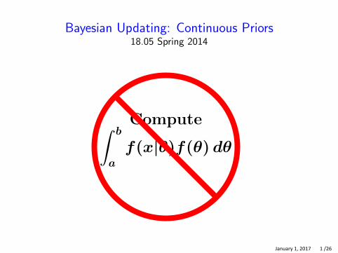
Beta distribution Beta(a, b) has density

(a + b − 1)!f (θ) = θa−1(1 − θ)b−1

(a − 1)!(b − 1)!

http://mathlets.org/mathlets/beta-distribution/

Observation: The coefficient is a normalizing factor, so if we have a pdf

f (θ) = cθa−1(1 − θ)b−1

then θ ∼ beta(a, b)

and (a + b − 1)!

c = (a − 1)!(b − 1)!

January 1, 2017 2 /26

Board question preamble: beta priors Suppose you are testing a new medical treatment with unknown probability of success θ. You don’t know that θ, but your prior belief is that it’s probably not too far from 0.5. You capture this intuition with a beta(5,5) prior on θ.

0.0 0.2 0.4 0.6 0.8 1.0

0.0

1.0

2.0

Beta(5,5) for θ

To sharpen this distribution you take data and update the prior.

Question on next slide. January 1, 2017 3 /26

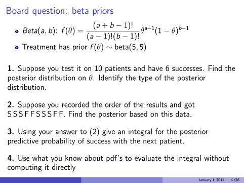
Board question: beta priors

(a + b − 1)!Beta(a, b): f (θ) = θa−1(1 − θ)b−1

(a − 1)!(b − 1)! Treatment has prior f (θ) ∼ beta(5, 5)

1. Suppose you test it on 10 patients and have 6 successes. Find the posterior distribution on θ. Identify the type of the posterior distribution.

2. Suppose you recorded the order of the results and got S S S F F S S S F F. Find the posterior based on this data.

3. Using your answer to (2) give an integral for the posterior predictive probability of success with the next patient.

4. Use what you know about pdf’s to evaluate the integral without computing it directly

January 1, 2017 4 /26

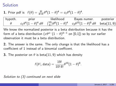
Solution 9!1. Prior pdf is f (θ) = θ4(1 − θ)4 = c1θ4(1 − θ)4 .4! 4!

hypoth. prior likelihood Bayes numer. posterior 10θ c1θ

4(1 − θ)4 dθ C )

θ6(1 − θ)4 c3θ10(1 − θ)8 dθ beta(11, 9)6

We know the normalized posterior is a beta distribution because it has the form of a beta distribution (cθa−(1 − θ)b−1 on [0,1]) so by our earlier observation it must be a beta distribution.

2. The answer is the same. The only change is that the likelihood has a coefficient of 1 instead of a binomial coefficent.

3. The posterior on θ is beta(11, 9) which has density

19! f (θ |, data) = θ10(1 − θ)8 .

10! 8!

Solution to (3) continued on next slide

January 1, 2017 5 /26

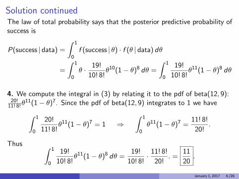
Solution continued The law of total probability says that the posterior predictive probability of success is

1 1

P(success | data) = f (success | θ) · f (θ | data) dθ 0 1 1 19!

1 1 19! = θ · θ10(1 − θ)8 dθ = θ11(1 − θ)8 dθ

10! 8! 10! 8! 0 0

4. We compute the integral in (3) by relating it to the pdf of beta(12, 9): 20! θ11(1 − θ)7 . Since the pdf of beta(12, 9) integrates to 1 we have 11! 8!

1 1 20! θ11(1 − θ)7 = 1 ⇒

1 1

θ11(1 − θ)7 = 11! 8!

. 0 11! 8! 0 20!

Thus 1 1 19! θ11(1 − θ)8 dθ =

19! · 11! 8! . = 11

. 0 10! 8! 10! 8! 20! 20

January 1, 2017 6 /26

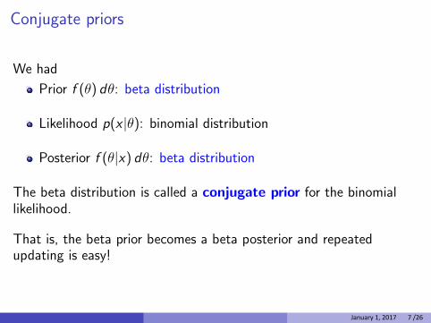
Conjugate priors

We had

Prior f (θ) dθ: beta distribution

Likelihood p(x |θ): binomial distribution

Posterior f (θ|x) dθ: beta distribution

The beta distribution is called a conjugate prior for the binomial likelihood.

That is, the beta prior becomes a beta posterior and repeated updating is easy!

January 1, 2017 7 /26

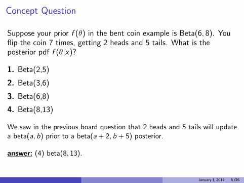
Concept Question

Suppose your prior f (θ) in the bent coin example is Beta(6, 8). You flip the coin 7 times, getting 2 heads and 5 tails. What is the posterior pdf f (θ|x)?

1. Beta(2,5)

2. Beta(3,6)

3. Beta(6,8)

4. Beta(8,13)

We saw in the previous board question that 2 heads and 5 tails will update a beta(a, b) prior to a beta(a + 2, b + 5) posterior.

answer: (4) beta(8, 13).

January 1, 2017 8 /26

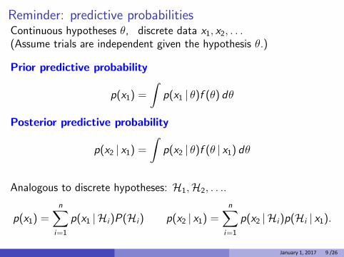
Reminder: predictive probabilities Continuous hypotheses θ, discrete data x1, x2, . . . (Assume trials are independent given the hypothesis θ.)

Prior predictive probability 1

p(x1) = p(x1 | θ)f (θ) dθ

Posterior predictive probability 1

p(x2 | x1) = p(x2 | θ)f (θ | x1) dθ

Analogous to discrete hypotheses: H1, H2, . . ..

n n

p(x1) = 1

p(x1 |Hi )P(Hi ) p(x2 | x1) = 1

p(x2 |Hi )p(Hi | x1). i=1 i=1

January 1, 2017 9 /26

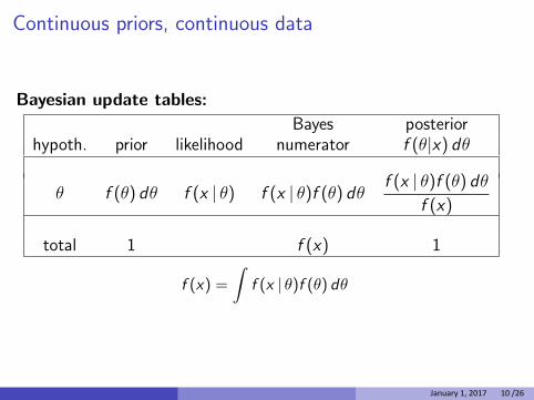
Continuous priors, continuous data

Bayesian update tables:

hypoth. prior likelihood Bayes

numerator posterior f (θ|x) dθ

θ f (θ) dθ f (x | θ) f (x | θ)f (θ) dθ f (x | θ)f (θ) dθ

f (x)

total 1 f (x) 1 1

f (x) = f (x | θ)f (θ) dθ

January 1, 2017 10 /26

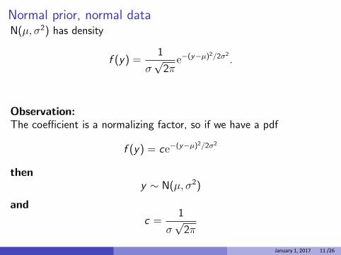
Normal prior, normal data N(µ, σ2) has density

1 −(y−µ)2/2σ2 f (y) = √ e .

σ 2π

Observation: The coefficient is a normalizing factor, so if we have a pdf

−(y −µ)2/2σ2 f (y) = ce

then y ∼ N(µ, σ2)

and 1

c = √ σ 2π

January 1, 2017 11 /26

Board question: normal prior, normal data

−(y−µ)2/2σ2 N(µ, σ2) has pdf: f (y) = √

1 e .

σ 2π Suppose our data follows a N(θ, 4) distribution with unknown mean θ and variance 4. That is

f (x | θ) = pdf of N(θ, 4)

Suppose our prior on θ is N(3, 1).

Suppose we obtain data x1 = 5.

1. Use the data to find the posterior pdf for θ.

Write out your tables clearly. Use (and understand) infinitesimals.

You will have to remember how to complete the square to do the updating!

January 1, 2017 12 /26

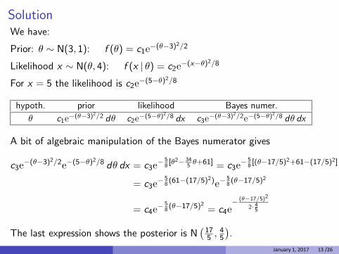
Solution We have:

−(θ−3)2/2Prior: θ ∼ N(3, 1): f (θ) = c1e−(x−θ)2/8Likelihood x ∼ N(θ, 4): f (x | θ) = c2e

−(5−θ)2/8For x = 5 the likelihood is c2e

hypoth. prior likelihood Bayes numer. θ c1e

−(θ−3)2/2 dθ c2e−(5−θ)2/8 dx c3e

−(θ−3)2/2e−(5−θ)2 /8 dθ dx

A bit of algebraic manipulation of the Bayes numerator gives

[θ2− 34−(θ−3)2/2 − 5 θ+61] − 5 [(θ−17/5)2+61−(17/5)2]c3e e −(5−θ)2/8 dθ dx = c3e 8 5 = c3e 8

− 5 (61−(17/5)2) − 5 (θ−17/5)2 = c3e 8 e 8

(θ−17/5)2

− 5 (θ−17/5)2 − 2· 4

= c4e 8 = c4e 5

). 4The last expression shows the posterior is N

C17 5 , 5

January 1, 2017 13 /26

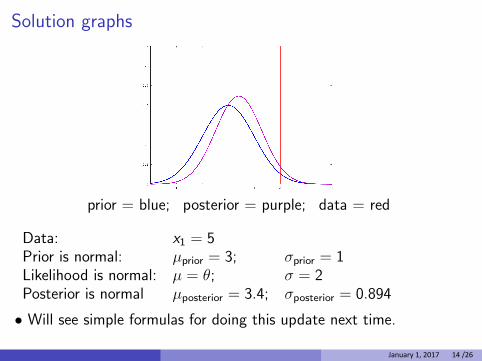
Solution graphs

prior = blue; posterior = purple; data = red

Data: x1 = 5 Prior is normal: µprior = 3; σprior = 1 Likelihood is normal: µ = θ; σ = 2 Posterior is normal µposterior = 3.4; σposterior = 0.894

• Will see simple formulas for doing this update next time.

January 1, 2017 14 /26

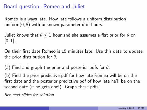
Board question: Romeo and Juliet

Romeo is always late. How late follows a uniform distribution uniform(0, θ) with unknown parameter θ in hours.

Juliet knows that θ ≤ 1 hour and she assumes a flat prior for θ on [0, 1].

On their first date Romeo is 15 minutes late. Use this data to update the prior distribution for θ.

(a) Find and graph the prior and posterior pdfs for θ.

(b) Find the prior predictive pdf for how late Romeo will be on the first date and the posterior predictive pdf of how late he’ll be on the second date (if he gets one!). Graph these pdfs.

See next slides for solution

January 1, 2017 15 /26

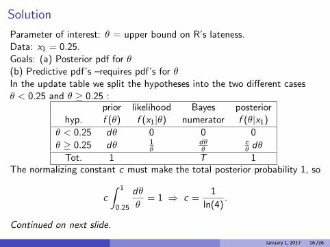
Solution

Parameter of interest: θ = upper bound on R’s lateness. Data: x1 = 0.25. Goals: (a) Posterior pdf for θ (b) Predictive pdf’s –requires pdf’s for θ In the update table we split the hypotheses into the two different cases θ < 0.25 and θ ≥ 0.25 :

prior likelihood Bayes posterior hyp. f (θ) f (x1|θ) numerator f (θ|x1)

θ < 0.25 θ ≥ 0.25

dθ dθ

0 1 θ

0 dθ θ

0 c θ dθ

Tot. 1 T 1 The normalizing constant c must make the total posterior probability 1, so

1 1 dθ 1 c = 1 ⇒ c = .

θ ln(4)0.25

Continued on next slide.

January 1, 2017 16 /26

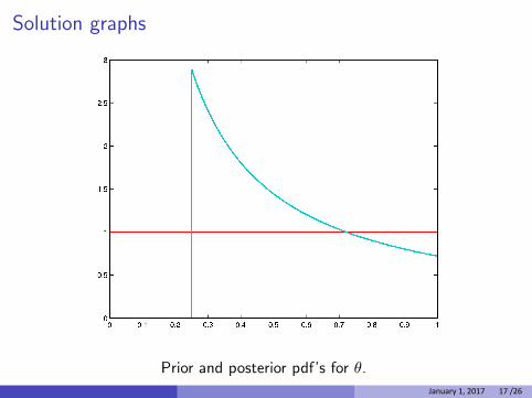
Solution graphs

Prior and posterior pdf’s for θ. January 1, 2017 17 /26

Solution graphs continued

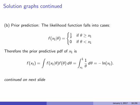
(b) Prior prediction: The likelihood function falls into cases: �

1 θ if θ ≥ x1

f (x1|θ) = 0 if θ < x1

Therefore the prior predictive pdf of x1 is

1 1 1 1 f (x1) = f (x1|θ)f (θ) dθ = dθ = − ln(x1).

θx1

continued on next slide

January 1, 2017 18 /26

�

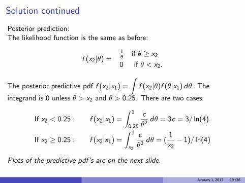
Solution continued

Posterior prediction: The likelihood function is the same as before:

1 if θ ≥ x2θf (x2|θ) = 0 if θ < x2.

1 The posterior predictive pdf f (x2|x1) = f (x2|θ)f (θ|x1) dθ. The

integrand is 0 unless θ > x2 and θ > 0.25. There are two cases:

1 1 c If x2 < 0.25 : f (x2|x1) = dθ = 3c = 3/ ln(4).

0.25 θ2

1 1 c 1 If x2 ≥ 0.25 : f (x2|x1) = dθ = ( − 1)/ ln(4)

θ2 x2x2

Plots of the predictive pdf’s are on the next slide.

January 1, 2017 19 /26

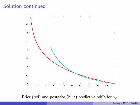
Solution continued

Prior (red) and posterior (blue) predictive pdf’s for x2

January 1, 2017 20 /26

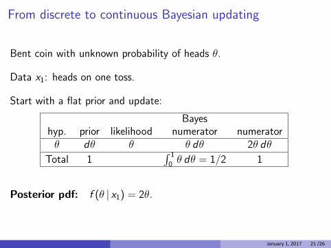
From discrete to continuous Bayesian updating

Bent coin with unknown probability of heads θ.

Data x1: heads on one toss.

Start with a flat prior and update:

hyp. prior likelihood Bayes

numerator numerator θ dθ θ θ dθ 2θ dθ

Total 1 J 1 0 θ dθ = 1/2 1

Posterior pdf: f (θ | x1) = 2θ.

January 1, 2017 21 /26

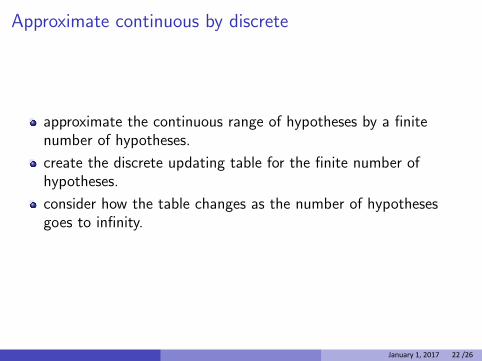
Approximate continuous by discrete

approximate the continuous range of hypotheses by a finite number of hypotheses.

create the discrete updating table for the finite number of hypotheses.

consider how the table changes as the number of hypotheses goes to infinity.

January 1, 2017 22 /26

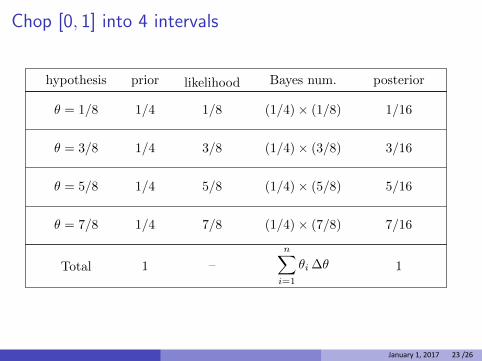
Chop [0, 1] into 4 intervals

hypothesis prior likelihood Bayes num. posterior

Total 1 –

n∑

i=1

θi ∆θ 1

1/4

θ = 1/8 1/8 (1/4) × (1/8) 1/16

1/4

θ = 3/8 3/8 (1/4) × (3/8) 3/161/4

θ = 5/8 5/8 (1/4) × (5/8) 5/16

1/4

θ = 7/8 7/8 (1/4) × (7/8) 7/16

January 1, 2017 23 /26

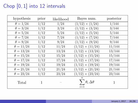
Chop [0, 1] into 12 intervals

hypothesis prior likelihood Bayes num. posterior

Total 1 –

n∑

i=1

θi ∆θ 1

1/12

θ = 1/24 1/24 (1/12)× (1/24) 1/144

1/12

θ = 3/24 3/24 (1/12)× (3/24) 3/144

1/12

θ = 5/24 5/24 (1/12)× (5/24) 5/144

1/12

θ = 7/24 7/24 (1/12)× (7/24) 7/144

1/12

θ = 9/24 9/24 (1/12)× (9/24) 9/144

1/12

θ = 11/24 11/24 (1/12)× (11/24) 11/1441/12

θ = 13/24 13/24 (1/12)× (13/24) 13/144

1/12

θ = 15/24 15/24 (1/12)× (15/24) 15/144

1/12

θ = 17/24 17/24 (1/12)× (17/24) 17/144

1/12

θ = 19/24 19/24 (1/12)× (19/24) 19/144

1/12

θ = 21/24 21/24 (1/12)× (21/24) 21/144

1/12

θ = 23/24 23/24 (1/12)× (23/24) 23/144

January 1, 2017 24 /26

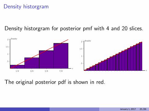
Density historgram

Density historgram for posterior pmf with 4 and 20 slices.

x

density

1/8 3/8 5/8 7/8

.5

1

1.5

2

x

density

.5

1

1.5

2

The original posterior pdf is shown in red.

January 1, 2017 25 /26

MIT OpenCourseWarehttps://ocw.mit.edu

18.05 Introduction to Probability and StatisticsSpring 2014

For information about citing these materials or our Terms of Use, visit: https://ocw.mit.edu/terms.