Author's personal copy - 国立大学法人...
37
This article appeared in a journal published by Elsevier. The attached copy is furnished to the author for internal non-commercial research and education use, including for instruction at the authors institution and sharing with colleagues. Other uses, including reproduction and distribution, or selling or licensing copies, or posting to personal, institutional or third party websites are prohibited. In most cases authors are permitted to post their version of the article (e.g. in Word or Tex form) to their personal website or institutional repository. Authors requiring further information regarding Elsevier’s archiving and manuscript policies are encouraged to visit: http://www.elsevier.com/authorsrights
Transcript of Author's personal copy - 国立大学法人...

This article appeared in a journal published by Elsevier. The attachedcopy is furnished to the author for internal non-commercial researchand education use, including for instruction at the authors institution
and sharing with colleagues.
Other uses, including reproduction and distribution, or selling orlicensing copies, or posting to personal, institutional or third party
websites are prohibited.
In most cases authors are permitted to post their version of thearticle (e.g. in Word or Tex form) to their personal website orinstitutional repository. Authors requiring further information
regarding Elsevier’s archiving and manuscript policies areencouraged to visit:
http://www.elsevier.com/authorsrights
Author's personal copy
Available online at www.sciencedirect.com
ScienceDirect
Nuclear Physics B 880 (2014) 378–413
www.elsevier.com/locate/nuclphysb
Correlation functions of the half-infinite XXZspin chain with a triangular boundary
P. Baseilhac a, T. Kojima b,∗
a Laboratoire de Mathématiques et Physique Théorique CNRS/UMR 7350, Fédération Denis Poisson FR2964,Université de Tours, Parc de Grammont, 37200 Tours, France
b Department of Mathematics and Physics, Faculty of Engineering, Yamagata University, Jonan 4-3-16,Yonezawa 992-8510, Japan
Received 8 October 2013; accepted 14 January 2014
Available online 17 January 2014
Abstract
The half-infinite XXZ spin chain with a triangular boundary is considered in the massive regime. Twointegral representations of correlation functions are proposed using bosonization. Sufficient conditions suchthat the expressions for triangular boundary conditions coincide with those for diagonal boundary condi-tions are identified. As an application, summation formulae of the boundary expectation values 〈σa
1 〉 witha = z,± are obtained. Exploiting the spin-reversal property, relations between n-fold integrals of elliptictheta functions are extracted.© 2014 The Authors. Published by Elsevier B.V. This is an open access article under the CC BY license(http://creativecommons.org/licenses/by/3.0/). Funded by SCOAP3.
1. Introduction
Beyond the Ising model, a large class of solvable lattice models have been discovered. In thecontext of quantum integrable systems on the lattice, spin chains are among the most studiedexamples with applications which range from condensed matter to high energy physics. Givena Hamiltonian, finding analytical expressions for the exact spectrum, identifying the structureof the space of the eigenvectors and deriving explicit expressions for correlation functions are
* Corresponding author.E-mail addresses: [email protected] (P. Baseilhac), [email protected] (T. Kojima).
http://dx.doi.org/10.1016/j.nuclphysb.2014.01.0110550-3213/© 2014 The Authors. Published by Elsevier B.V. This is an open access article under the CC BY license
(http://creativecommons.org/licenses/by/3.0/). Funded by SCOAP3.
Author's personal copy
P. Baseilhac, T. Kojima / Nuclear Physics B 880 (2014) 378–413 379
essential steps in the non-perturbative characterization of the system’s behavior which can becompared with experimental data.
Among the simplest examples considered in the literature, the XXZ spin chain with differ-ent boundary conditions has received particular attention. Over the years, different approacheshave been proposed in order to understand the Hamiltonian’s spectral problem and derive thecorrelation functions. For models with periodic boundary conditions, the spectral problem canbe handled by methods such as the Bethe ansatz (BA) [1], or the corner transfer matrix method(CTM) in the thermodynamic limit [2]. The computation of the correlation functions, however,is a much more difficult problem in general. Apart from the simplest example – namely theXXZ spin chain with periodic boundary condition – for which correlation functions have beenproposed by the quantum inverse scattering method (QISM) [4,5] arising from the BA, the gen-eralization of this result to models with higher symmetries requires a better understanding ofmathematical structures, for instance, of determinant formulae of scalar products that involvethe Bethe vectors [7] (see some recent progress in [8]). However, in the thermodynamic limit,this problem can be alternatively tackled using the q-vertex operator approach (VOA) [3] arisingfrom the CTM. The space of states is identified with the irreducible highest weight representa-tion of Uq(sl2) or higher rank quantum algebras. Correlation functions can be obtained usingbosonizations of the q-vertex operators for Uq(sl2) or higher rank quantum algebras [3,9–13].Either within the QISM or the VOA, correlation functions are obtained in the form of integralsof meromorphic functions in the thermodynamic limit.
The situation for integrable spin chains with open boundaries is more difficult. On one hand,for the finite XXZ open chain with diagonal boundaries [14], related non-diagonal boundaries[15,16] or q a root of unity [17], the BA makes it possible to derive the spectrum and the eigen-vectors1 [16]. In each case, the corresponding models are studied using Sklyanin’s general formu-lation of the BA applied to open boundary models [14]. On the other hand, in the thermodynamiclimit, the VOA has been applied to the half-infinite XXZ spin chain with a diagonal boundary [6].Although the hidden symmetry of this model was still unknown at that time,2 the diagonalizationof the Hamiltonian could still be achieved. Based on these results, the computation of correla-tion functions has been achieved for diagonal boundary conditions either using the BA [20] orusing the VOA in the thermodynamic limit [6]. Note that generalizations to models with highersymmetries have been studied for Uq(slN), etc. [21–23]. In the thermodynamic limit, when thecomparison is feasible the expressions obtained by both approaches essentially coincide.
In spite of these important developments, the computation of correlation functions of the XXZopen spin chain for more general boundary conditions has remained, up to now, essentially prob-lematic. On one hand, even in a simpler case such as the XXZ spin chain with triangular boundaryconditions for which the construction of the Bethe vector is feasible [24,25], it remains an openproblem in the QISM. On the other hand, in the thermodynamic limit the application of the VOArequires the prior knowledge of the vacuum eigenvectors of the Hamiltonian. Since 1994 [6],even for the simpler case of triangular boundary conditions the solution to this problem has beenunknown. However, a breakthrough was recently made in [27], which has opened the possibil-ity of computing correlation functions in the thermodynamic limit of the XXZ open spin chain.Namely, based on the so-called Onsager’s approach the structure of the eigenvectors of the finiteXXZ spin chain for any type of boundary conditions was interpreted within the representation
1 Note that recently, a modified BA approach has been considered which looks promising [18,19].2 Recently, the hidden symmetry of the spin chain with a diagonal and non-diagonal boundary has been identified: it is
associated with the augmented q-Onsager algebra and q-Onsager algebra, respectively [27].
Author's personal copy
380 P. Baseilhac, T. Kojima / Nuclear Physics B 880 (2014) 378–413
theory of the q-Onsager algebra [26,27]. In the thermodynamic limit, the q-Onsager algebra isrealized by quadratics of the q-vertex operators associated with Uq(sl2) [27] (see also [28] foran alternative derivation). As a consequence, vacuum eigenvectors of the Hamiltonian for a tri-angular boundary were constructed using the intertwining properties of the q-vertex operatorswith monomials of the q-Onsager basic generators [27]. The latter being expressed in terms ofUq(sl2) generators, the VOA can be applied in a straightforward manner.
The purpose of this paper is to present the first examples of correlation functions of the half-infinite XXZ open spin chain with a non-diagonal boundary, using the framework of the VOA.The results here presented extend the earlier studies [6,27]. Among the applications, closedformulae for the boundary expectation values of the spin operators are given and remarkableidentities between n-fold integrals of elliptic theta functions are exhibited. Here we focus ourattention on the simplest non-diagonal example, namely the half-infinite XXZ spin chain withupper or lower triangular boundary condition. We are interested in the Hamiltonian:
H(±)B = −1
2
∞∑k=1
(σx
k+1σxk + σ
y
k+1σyk + Δσz
k+1σzk
)− 1 − q2
4q
1 + r
1 − rσ z
1 − s
1 − rσ±
1 , (1.1)
where we have used the standard Pauli matrices
σx =(
0 11 0
), σ y =
(0 −i
i 0
), σ z =
(1 00 −1
),
σ+ =(
0 10 0
), σ− =
(0 01 0
). (1.2)
Here we consider the model in the limit of the half-infinite spin chain, in the massive regimewhere
Δ = q + q−1
2, −1 < q < 0, −1 � r � 1, s ∈ R. (1.3)
Since under conjugation of H(±)B by the spin-reversal operator ν = ∏∞
j=1 σxj the sign of the
boundary term is reversed, we can restrict our discussion to the boundary term − 1−q2
4q1+r1−r
� 0,or −1 � r � 1. Importantly, the two fundamental vacuum eigenvectors |±; i〉B (i = 0,1) for thetriangular boundary models H
(±)B were constructed in a recent paper [27]. For instance, for the
lower triangular boundary model H(−)B , the two fundamental vacuum eigenvectors3 are given by
q-exponentials of Uq(sl2) Chevalley generators acting on the vacuum eigenvectors |i〉B (i = 0,1)
of the model with a diagonal boundary (s = 0) [6]:
|−;0〉B = expq
(− s
qe0q
−h0
)|0〉B, |−;1〉B = expq−1
(− s
rf1
)|1〉B. (1.4)
Here we have used the q-exponential function
expq(x) =∞∑
n=0
qn(n−1)
2
[n]q ! xn. (1.5)
3 By definition [27], |±; i〉B (i = 0,1) are eigenvectors of the Hamiltonian (1.1), not to be confused with the objectscalled the pseudo-vacuum vectors that arise in the algebraic BA approach.

Author's personal copy
P. Baseilhac, T. Kojima / Nuclear Physics B 880 (2014) 378–413 381
In this paper we give the dual vacuum eigenvectors B 〈i;±| (i = 0,1) using the intertwiningproperties of the q-vertex operators of Uq(sl2). For instance, for the lower triangular boundary
model H(−)B , the two fundamental dual vacuum eigenvectors are given by
B〈0;−| = B〈0| expq−1
(s
qe0q
−h0
), B〈1;−| = B〈1| expq
(s
rf1
). (1.6)
Using these, we compute the integral representations of the correlation functions using thebosonizations. As a special case, the summation formulae of the boundary expectation valuesof the spin operators are derived:
B〈0;−|σz1 |−;0〉B
B〈0;−|−;0〉B = −1 − 2(1 − r)2∞∑
n=1
(−q2)n
(1 − rq2n)2, (1.7)
B〈0;−|σ+1 |−;0〉B
B〈0;−|−;0〉B = s
(2 + (1 − r)
∞∑n=1
(−q2)n 2q2n − r(1 + q4n)
(1 − rq2n)2
), (1.8)
B〈0;−|σ−1 |−;0〉B
B〈0;−|−;0〉B = 0. (1.9)
This is one of the main result of this paper. Also, sufficient conditions such that the correlationfunctions for a triangular boundary coincide with those for a diagonal boundary are derived. Asa special case, we have the following equation for the diagonal matrix σz:
B〈i;±|σzM · · ·σz
2 σz1 |±; i〉B
B〈i;±|±; i〉B = B〈i|σzM · · ·σz
2 σz1 |i〉B
B〈i|i〉B . (1.10)
Finally, let us also mention that provided a suitable change of the boundary parameters, theHamiltonian of the two triangular boundary models H
(±)B exchange each other under the action
of the spin-reversal operator ν. As a consequence, correlation functions of the lower triangularmodel H
(−)B are related to those of the upper triangular model H
(+)B . Using this property, for
instance we have the following identity of multiple integrals:
(q4;q4)4∞(q2;q2)8∞
1 − z2
Θq4(z2)
(2 + 1 − z/r
z
∞∑n=1
(−q2)n (z − z−1) − (1 + q4n)/r + (z + z−1)q2n
(1 − q2nz/r)(1 − q2n/rz)
)
=(
q2∫ ∫ ∫
C0
−∫ ∫ ∫
C1
)
×3∏
a=1
dwa
2π√−1
q2(1 − 1/rz)(1 − q/rw3)∏2
a=1(1 − q2/zwa)
w22w
33(1 − q2w1/w2)(1 − q4/w1w2)
∏2a=1(1 − q2/rwa)
× Θq2(w1w2)Θq2(w2/w1)Θq2(zw3/q)Θq2(qw3/z)∏3
a=1 Θq4(w2a/q
2)∏2a=1 Θq2(waw3/q2)Θq2(wa/qw3)Θq2(waz)Θq2(wa/z)
, (1.11)
where we have used the elliptic theta function
Θp(z) = (p;p)∞(z;p)∞(p/z;p)∞, (z;p)∞ =∞∏
n=0
(1 − pnz
). (1.12)

Author's personal copy
382 P. Baseilhac, T. Kojima / Nuclear Physics B 880 (2014) 378–413
Here the integration contours Cl = C(+,1)l (l = 0,1) are simple closed curves given below (4.58),
(4.60).The plan of this paper is as follows. In Section 2, the half-infinite XXZ spin chain with a
triangular boundary is formulated using the q-vertex operator approach. In Section 3, we reviewthe realizations of the vacuum eigenvectors and their duals [6,27]. In Section 4, two integral rep-resentations of the correlation functions are calculated using bosonizations. As a straightforwardapplication, summation formulae of the boundary expectation values 〈σ±
1 〉 are obtained. Also, wederive identities between multiple integrals of elliptic theta functions from spin-reversal property.For each type of integral representation, a sufficient condition such that the expression for a tri-angular boundary condition coincides with those for a diagonal boundary condition is identified.Concluding remarks are given in Section 5. In Appendix A we recall some basic facts about thequantum group Uq(sl2) and fix the notations used in the main text. In Appendix B we recall thebosonizations of Uq(sl2) and the q-vertex operators. In Appendix C we summarize convenientformulae for the calculations of the vacuum expectation values.
2. The half-infinite XXZ spin chain with a triangular boundary
In this section we give a mathematical formulation of the half-infinite XXZ spin chain with atriangular boundary, based on the q-vertex operator approach [6].
2.1. Physical picture
In this section we sketch a physical picture of our problem. In Sklyanin’s framework [14],the transfer matrix T
(±,i)B (ζ ; r, s) that is a generating function of the Hamiltonian H
(±)B (1.1) is
introduced. Basically, it is built from two objects: the R-matrix and the K-matrix. For the model(1.1), one introduces the R-matrix R(ζ ) defined as:
R(ζ ) = 1
κ(ζ )
⎛⎜⎜⎜⎝1
(1−ζ 2)q
1−q2ζ 2(1−q2)ζ
1−q2ζ 2
(1−q2)ζ
1−q2ζ 2(1−ζ 2)q
1−q2ζ 2
1
⎞⎟⎟⎟⎠ , (2.1)
where we have set
κ(ζ ) = ζ(q4ζ 2;q4)∞(q2/ζ 2;q4)∞(q4/ζ 2;q4)∞(q2ζ 2;q4)∞
, (z;p)∞ =∞∏
n=0
(1 − pnz
). (2.2)
Let {v+, v−} denote the natural basis of V = C2. When viewed as an operator on V ⊗V , the ma-trix elements of R(ζ ) ∈ End(V ⊗ V ) are given by R(ζ )vε1 ⊗ vε2 = ∑
ε′1,ε
′2=± vε′
1⊗ vε′
2R(ζ )
ε1ε2ε′
1ε′2,
where the ordering of the index is given by v+ ⊗v+, v+ ⊗v−, v− ⊗v+, v− ⊗v−. As usual, whencopies Vj of V are involved, Rij (ζ ) acts as R(ζ ) on the i-th and j -th components and as identityelsewhere. The R-matrix R(ζ ) satisfies the Yang–Baxter equation.
R12(ζ1/ζ2)R13(ζ1/ζ3)R23(ζ2/ζ3) = R23(ζ2/ζ3)R13(ζ1/ζ3)R12(ζ1/ζ2). (2.3)
The normalization factor (2.2) is determined by the following unitarity and crossing symmetryconditions:
R12(ζ )R21(ζ−1) = 1, R(ζ )
ε′2ε1
ε2ε′1= R
(−q−1ζ−1)−ε′1ε
′2−ε1ε2. (2.4)
Author's personal copy
P. Baseilhac, T. Kojima / Nuclear Physics B 880 (2014) 378–413 383
Also, we introduce the triangular K-matrix K(±)(ζ ) = K(±)(ζ ; r, s) [29,30] by
K(+)(ζ ; r, s) = ϕ(ζ 2; r)ϕ(ζ−2; r)
( 1−rζ 2
ζ 2−r
sζ(ζ 2−ζ−2)
ζ 2−r
0 1
), (2.5)
K(−)(ζ ; r, s) = ϕ(ζ 2; r)ϕ(ζ−2; r)
( 1−rζ 2
ζ 2−r0
sζ(ζ 2−ζ−2)
ζ 2−r1
), (2.6)
where we have set
ϕ(z; r) = (q4rz;q4)∞(q6z2;q8)∞(q2rz;q4)∞(q8z2;q8)∞
. (2.7)
When viewed as an operator on V , the matrix elements of K(±)(ζ ) ∈ End(V ) are given byK(±)(ζ )vε = ∑
ε′=± vε′K(±)(ζ )εε′ , where the ordering of the index is given by v+, v−. As usual,
when copies Vj of V are involved, K(±)j (ζ ) acts as K(±)(ζ ) on the j -th component and as
identity elsewhere. The K-matrix K(±)(ζ ) satisfies the boundary Yang–Baxter equation (alsocalled the reflection equation):
K(±)2 (ζ2)R21(ζ1ζ2)K
(±)1 (ζ1)R12(ζ1/ζ2) = R21(ζ1/ζ2)K
(±)1 (ζ1)R12(ζ1ζ2)K
(±)2 (ζ2). (2.8)
The normalization factor (2.7) is determined by the following boundary unitarity and boundarycrossing symmetry [30]:
K(±)(ζ )K(±)(ζ−1) = 1,
K(±)(−q−1ζ−1)ε2
ε1=
∑ε′
1,ε′2=±
R(−qζ 2)−ε1ε2
ε′1−ε′
2K(±)(ζ )
ε′1
ε′2. (2.9)
The K(±)(ζ ; r, s) defined in (2.5) and (2.6) give general scalar triangular solutions of (2.8) and(2.9).
In Sklyanin’s framework, defined on a finite lattice the transfer matrix is built from a fi-nite number of R-matrix [14]. In order to formulate the model (1.1), an infinite combination ofR-matrices [6] is considered in T
(±,i)B (ζ ; r, s). Generally speaking infinite combinations of the
R-matrix are not free from the difficulty of divergence, however we know two useful conceptsto study infinite combinations of the R-matrix. One is the corner transfer matrix (CTM) intro-duced by Baxter [2]. The other is the q-vertex operator introduced by Baxter [35] and Jimbo,Miwa, and Nakayashiki [37]. The CTM for Uq(sl2) [38] gives a supporting argument for themathematical formulation presented in the next section, that is free from the difficulty of diver-gences. Following the strategy summarized in [6,37], let us recall the mathematical formulationof the q-vertex operators and the transfer matrix. Consider the infinite dimensional vector space· · · ⊗ V3 ⊗ V2 ⊗ V1 on which the Hamiltonian (1.1) acts. Let us introduce the subspace H(i)
(i = 0,1) of the half-infinite spin chain by
H(i) = Span{· · · ⊗ vp(N) ⊗ · · · ⊗ vp(2) ⊗ vp(1)
∣∣ p(N) = (−1)N+i (N 1)}, (2.10)
where p : N → {±}. We introduce the q-vertex operator Φ(1−i,i)ε (ζ ) and the dual q-vertex op-
erator Φ∗(1−i,i)ε (ζ ) for ε = ± which act on the space H(i) (i = 0,1). Their matrix elements are
given by products of the R-matrix as follows:
Author's personal copy
384 P. Baseilhac, T. Kojima / Nuclear Physics B 880 (2014) 378–413
(Φ(1−i,i)
ε (ζ ))···p(N)′···p(2)′p(1)′···p(N)···p(2) p(1)
= limN→∞
∑μ(1),μ(2),...,μ(N)=±
N∏j=1
R(ζ )μ(j) p(j)′μ(j−1) p(j), (2.11)
(Φ∗(1−i,i)
ε (ζ ))···p(N)′···p(2)′p(1)′···p(N)···p(2) p(1)
= limN→∞
∑μ(1),μ(2),...,μ(N)=±
N∏j=1
R(ζ )p(j)′ μ(j−1)
p(j) μ(j) , (2.12)
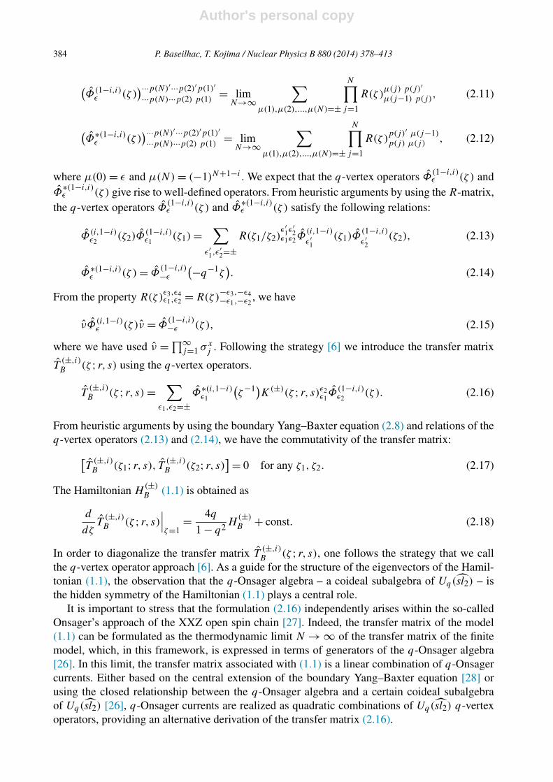
where μ(0) = ε and μ(N) = (−1)N+1−i . We expect that the q-vertex operators Φ(1−i,i)ε (ζ ) and
Φ∗(1−i,i)ε (ζ ) give rise to well-defined operators. From heuristic arguments by using the R-matrix,
the q-vertex operators Φ(1−i,i)ε (ζ ) and Φ
∗(1−i,i)ε (ζ ) satisfy the following relations:
Φ(i,1−i)ε2
(ζ2)Φ(1−i,i)ε1
(ζ1) =∑
ε′1,ε
′2=±
R(ζ1/ζ2)ε′
1ε′2
ε1ε2Φ(i,1−i)
ε′1
(ζ1)Φ(1−i,i)
ε′2
(ζ2), (2.13)
Φ∗(1−i,i)ε (ζ ) = Φ
(1−i,i)−ε
(−q−1ζ). (2.14)
From the property R(ζ )ε3,ε4ε1,ε2 = R(ζ )
−ε3,−ε4−ε1,−ε2, we have
νΦ(i,1−i)ε (ζ )ν = Φ
(1−i,i)−ε (ζ ), (2.15)
where we have used ν = ∏∞j=1 σx
j . Following the strategy [6] we introduce the transfer matrix
T(±,i)B (ζ ; r, s) using the q-vertex operators.
T(±,i)B (ζ ; r, s) =
∑ε1,ε2=±
Φ∗(i,1−i)ε1
(ζ−1)K(±)(ζ ; r, s)ε2
ε1Φ(1−i,i)
ε2(ζ ). (2.16)
From heuristic arguments by using the boundary Yang–Baxter equation (2.8) and relations of theq-vertex operators (2.13) and (2.14), we have the commutativity of the transfer matrix:[
T(±,i)B (ζ1; r, s), T (±,i)
B (ζ2; r, s)] = 0 for any ζ1, ζ2. (2.17)
The Hamiltonian H(±)B (1.1) is obtained as
d
dζT
(±,i)B (ζ ; r, s)
∣∣∣ζ=1
= 4q
1 − q2H
(±)B + const. (2.18)
In order to diagonalize the transfer matrix T(±,i)B (ζ ; r, s), one follows the strategy that we call
the q-vertex operator approach [6]. As a guide for the structure of the eigenvectors of the Hamil-tonian (1.1), the observation that the q-Onsager algebra – a coideal subalgebra of Uq(sl2) – isthe hidden symmetry of the Hamiltonian (1.1) plays a central role.
It is important to stress that the formulation (2.16) independently arises within the so-calledOnsager’s approach of the XXZ open spin chain [27]. Indeed, the transfer matrix of the model(1.1) can be formulated as the thermodynamic limit N → ∞ of the transfer matrix of the finitemodel, which, in this framework, is expressed in terms of generators of the q-Onsager algebra[26]. In this limit, the transfer matrix associated with (1.1) is a linear combination of q-Onsagercurrents. Either based on the central extension of the boundary Yang–Baxter equation [28] orusing the closed relationship between the q-Onsager algebra and a certain coideal subalgebraof Uq(sl2) [26], q-Onsager currents are realized as quadratic combinations of Uq(sl2) q-vertexoperators, providing an alternative derivation of the transfer matrix (2.16).
Author's personal copy
P. Baseilhac, T. Kojima / Nuclear Physics B 880 (2014) 378–413 385
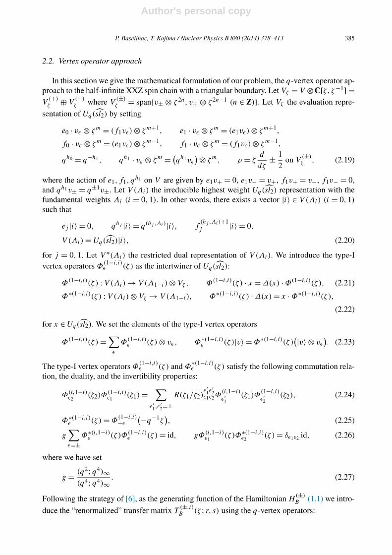
2.2. Vertex operator approach
In this section we give the mathematical formulation of our problem, the q-vertex operator ap-proach to the half-infinite XXZ spin chain with a triangular boundary. Let Vζ = V ⊗C[ζ, ζ−1] =V
(+)ζ ⊕ V
(−)ζ where V
(±)ζ = span{v± ⊗ ζ 2n, v∓ ⊗ ζ 2n−1 (n ∈ Z)}. Let Vζ the evaluation repre-
sentation of Uq(sl2) by setting
e0 · vε ⊗ ζm = (f1vε) ⊗ ζm+1, e1 · vε ⊗ ζm = (e1vε) ⊗ ζm+1,
f0 · vε ⊗ ζm = (e1vε) ⊗ ζm−1, f1 · vε ⊗ ζm = (f1vε) ⊗ ζm−1,
qh0 = q−h1, qh1 · vε ⊗ ζm = (qh1vε
)⊗ ζm, ρ = ζd
dζ± 1
2on V
(±)ζ , (2.19)
where the action of e1, f1, qh1 on V are given by e1v+ = 0, e1v− = v+, f1v+ = v−, f1v− = 0,
and qh1v± = q±1v±. Let V (Λi) the irreducible highest weight Uq(sl2) representation with thefundamental weights Λi (i = 0,1). In other words, there exists a vector |i〉 ∈ V (Λi) (i = 0,1)
such that
ej |i〉 = 0, qhj |i〉 = q(hj ,Λi)|i〉, f(hj ,Λi)+1j |i〉 = 0,
V (Λi) = Uq(sl2)|i〉, (2.20)
for j = 0,1. Let V ∗(Λi) the restricted dual representation of V (Λi). We introduce the type-Ivertex operators Φ
(1−i,i)ε (ζ ) as the intertwiner of Uq(sl2):
Φ(1−i,i)(ζ ) : V (Λi) → V (Λ1−i ) ⊗ Vζ , Φ(1−i,i)(ζ ) · x = Δ(x) · Φ(1−i,i)(ζ ), (2.21)
Φ∗(1−i,i)(ζ ) : V (Λi) ⊗ Vζ → V (Λ1−i ), Φ∗(1−i,i)(ζ ) · Δ(x) = x · Φ∗(1−i,i)(ζ ),
(2.22)
for x ∈ Uq(sl2). We set the elements of the type-I vertex operators
Φ(1−i,i)(ζ ) =∑
ε
Φ(1−i,i)ε (ζ ) ⊗ vε, Φ∗(1−i,i)
ε (ζ )|v〉 = Φ∗(1−i,i)(ζ )(|v〉 ⊗ vε
). (2.23)
The type-I vertex operators Φ(1−i,i)ε (ζ ) and Φ
∗(1−i,i)ε (ζ ) satisfy the following commutation rela-
tion, the duality, and the invertibility properties:
Φ(i,1−i)ε2
(ζ2)Φ(1−i,i)ε1
(ζ1) =∑
ε′1,ε
′2=±
R(ζ1/ζ2)ε′
1ε′2
ε1ε2Φ(i,1−i)
ε′1
(ζ1)Φ(1−i,i)
ε′2
(ζ2), (2.24)
Φ∗(1−i,i)ε (ζ ) = Φ
(1−i,i)−ε
(−q−1ζ), (2.25)
g∑ε=±
Φ∗(i,1−i)ε (ζ )Φ(1−i,i)
ε (ζ ) = id, gΦ(i,1−i)ε1
(ζ )Φ∗(1−i,i)ε2
(ζ ) = δε1ε2 id, (2.26)
where we have set
g = (q2;q4)∞(q4;q4)∞
. (2.27)
Following the strategy of [6], as the generating function of the Hamiltonian H(±)B (1.1) we intro-
duce the “renormalized” transfer matrix T(±,i)B (ζ ; r, s) using the q-vertex operators:

Author's personal copy
386 P. Baseilhac, T. Kojima / Nuclear Physics B 880 (2014) 378–413
T(±,i)B (ζ ; r, s) = g
∑ε1,ε2=±
Φ∗(i,1−i)ε1
(ζ−1)K(±)(ζ ; r, s)ε2
ε1Φ(1−i,i)
ε2(ζ ). (2.28)
From the boundary Yang–Baxter equation and the properties of the q-vertex operators (2.8),(2.9), (2.24), (2.25), (2.26), we have the following properties of the “renormalized” transfer ma-trix: [
T(±,i)B (ζ1; r, s), T (±,i)
B (ζ2; r, s)] = 0 for any ζ1, ζ2, (2.29)
T(±,i)B (1; r, s) = id, T
(±,i)B (ζ ; r, s)T (±,i)
B
(ζ−1; r, s) = id. (2.30)
T(±,i)B
(−q−1ζ−1; r, s) = T(±,i)B (ζ ; r, s). (2.31)
Following the strategy in [3,6,37] and the CTM argument for Uq(sl2) [38], as well as the al-ternative support within Onsager’s framework [27], we study our problem upon the followingidentification:
T(±,i)B (ζ ; r, s) = T
(±,i)B (ζ ; r, s), Φ(1−i,i)
ε (ζ ) = Φ(1−i,i)ε (ζ ),
Φ∗(1−i,i)ε (ζ ) = Φ∗(1−i,i)
ε (ζ ). (2.32)
The point of using the q-vertex operators Φ(1−i,i)ε (ζ ), Φ
∗(1−i,i)ε (ζ ) associated with Uq(sl2) is
that they are well-defined objects, free from the difficulty of divergence. In addition, they are theunique solution of the intertwining relations defining the q-vertex operators of the q-Onsageralgebra (see [27] for details), which characterizes the hidden non-Abelian symmetry of (1.1).
Finally, let us describe the spin-reversal property. Let ν : V (Λ0) → V (Λ1) be the vector-spaceisomorphism corresponding to the Dynkin diagram symmetry [3]. Then we have
ν−1ej ν = e1−j , ν−1fjν = f1−j , ν−1qhj ν = qh1−j . (2.33)
Moreover we have
νΦ(0,1)ε (ζ )ν = Φ
(1,0)−ε (ζ ), (2.34)
which gives the same relation as (2.15). The q-vertex operator Φ(1−i,i)ε (ζ ) has a bosonization
summarized in Appendix B. Note that we have two bosonizations of the q-vertex operator basedon (2.34). Noting the relation
σxK(±)(ζ ; r, s)σ x = Λ(ζ ; r)K(∓)(ζ ;1/r,−s/r), (2.35)
where we have used
Λ(ζ ; r) = 1
ζ 2
Θq4(rζ 2)Θq4(q2rζ−2)
Θq4(rζ−2)Θq4(q2rζ 2), (2.36)
we find that
ν−1T(±,1)B (ζ ; r, s)ν = Λ(ζ ; r)T (∓,0)
B (ζ ;1/r,−s/r). (2.37)
In the next section we describe the vacuum eigenvectors |±; i〉B and their duals B 〈i;±| (i = 0,1)
such that
B〈i;±|T (±,i)B (ζ ; r, s) = B〈i;±|Λ(i)(ζ ; r), (2.38)
T(±,i)B (ζ ; r, s)|±; i〉B = Λ(i)(ζ ; r)|±; i〉B. (2.39)
Author's personal copy
P. Baseilhac, T. Kojima / Nuclear Physics B 880 (2014) 378–413 387
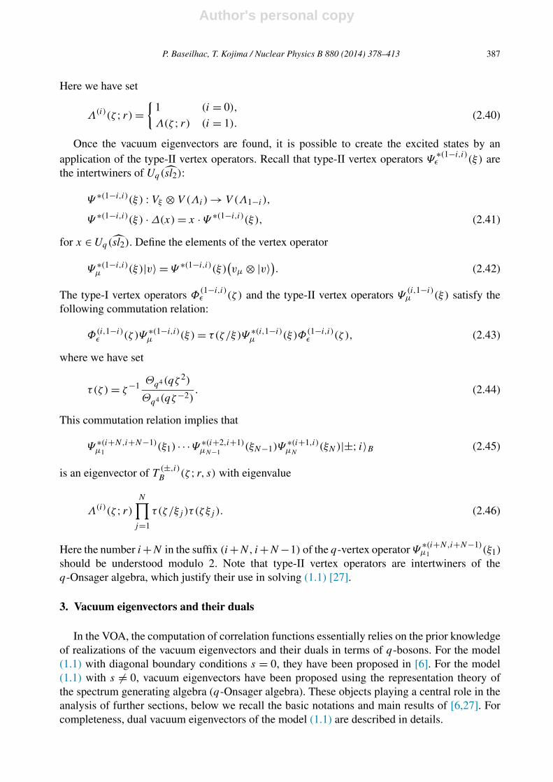
Here we have set
Λ(i)(ζ ; r) ={
1 (i = 0),
Λ(ζ ; r) (i = 1).(2.40)
Once the vacuum eigenvectors are found, it is possible to create the excited states by anapplication of the type-II vertex operators. Recall that type-II vertex operators Ψ
∗(1−i,i)ε (ξ) are
the intertwiners of Uq(sl2):
Ψ ∗(1−i,i)(ξ) : Vξ ⊗ V (Λi) → V (Λ1−i ),
Ψ ∗(1−i,i)(ξ) · Δ(x) = x · Ψ ∗(1−i,i)(ξ), (2.41)
for x ∈ Uq(sl2). Define the elements of the vertex operator
Ψ ∗(1−i,i)μ (ξ)|v〉 = Ψ ∗(1−i,i)(ξ)
(vμ ⊗ |v〉). (2.42)
The type-I vertex operators Φ(1−i,i)ε (ζ ) and the type-II vertex operators Ψ
(i,1−i)μ (ξ) satisfy the
following commutation relation:
Φ(i,1−i)ε (ζ )Ψ ∗(1−i,i)
μ (ξ) = τ(ζ/ξ)Ψ ∗(i,1−i)μ (ξ)Φ(1−i,i)
ε (ζ ), (2.43)
where we have set
τ(ζ ) = ζ−1 Θq4(qζ 2)
Θq4(qζ−2). (2.44)
This commutation relation implies that
Ψ ∗(i+N,i+N−1)μ1
(ξ1) · · ·Ψ ∗(i+2,i+1)μN−1
(ξN−1)Ψ∗(i+1,i)μN
(ξN)|±; i〉B (2.45)
is an eigenvector of T(±,i)B (ζ ; r, s) with eigenvalue
Λ(i)(ζ ; r)N∏
j=1
τ(ζ/ξj )τ (ζ ξj ). (2.46)
Here the number i+N in the suffix (i+N, i+N −1) of the q-vertex operator Ψ∗(i+N,i+N−1)μ1 (ξ1)
should be understood modulo 2. Note that type-II vertex operators are intertwiners of theq-Onsager algebra, which justify their use in solving (1.1) [27].
3. Vacuum eigenvectors and their duals
In the VOA, the computation of correlation functions essentially relies on the prior knowledgeof realizations of the vacuum eigenvectors and their duals in terms of q-bosons. For the model(1.1) with diagonal boundary conditions s = 0, they have been proposed in [6]. For the model(1.1) with s �= 0, vacuum eigenvectors have been proposed using the representation theory ofthe spectrum generating algebra (q-Onsager algebra). These objects playing a central role in theanalysis of further sections, below we recall the basic notations and main results of [6,27]. Forcompleteness, dual vacuum eigenvectors of the model (1.1) are described in details.
Author's personal copy
388 P. Baseilhac, T. Kojima / Nuclear Physics B 880 (2014) 378–413
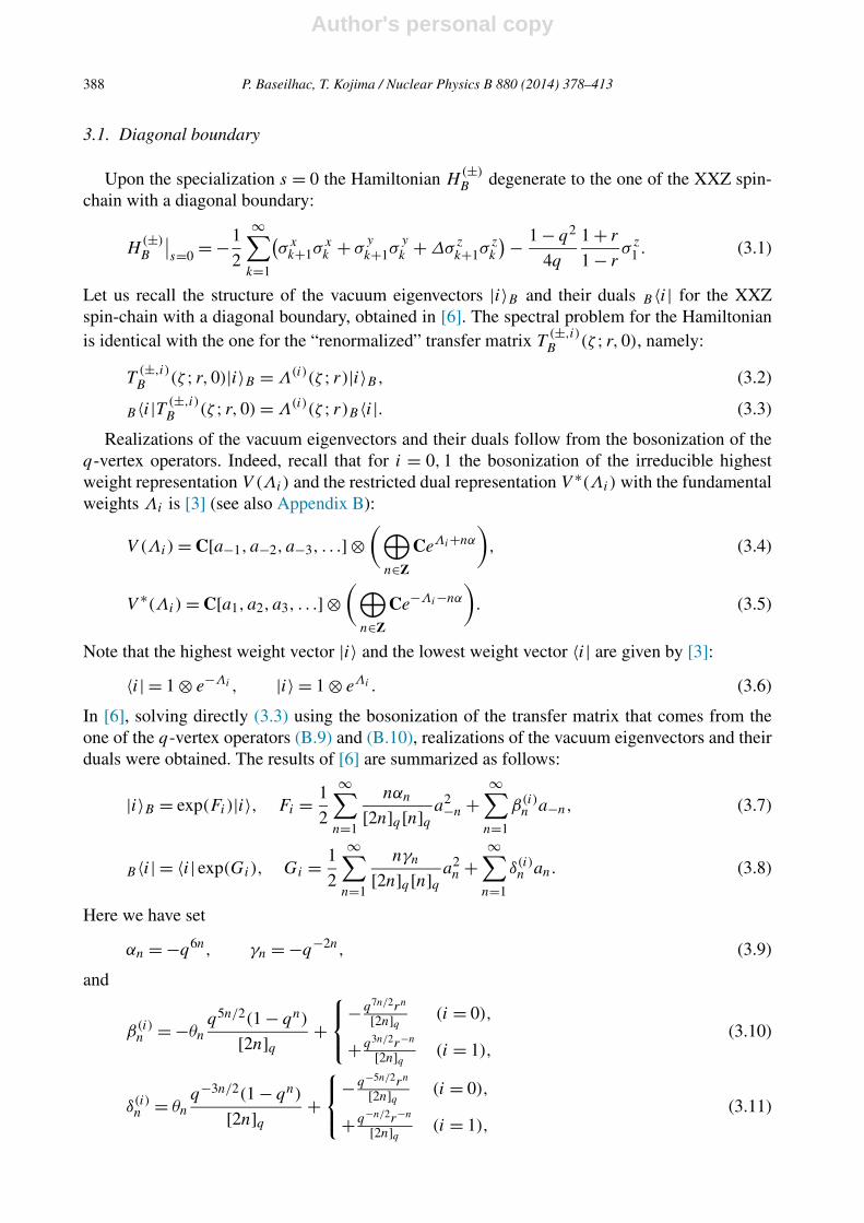
3.1. Diagonal boundary
Upon the specialization s = 0 the Hamiltonian H(±)B degenerate to the one of the XXZ spin-
chain with a diagonal boundary:
H(±)B
∣∣s=0 = −1
2
∞∑k=1
(σx
k+1σxk + σ
y
k+1σyk + Δσz
k+1σzk
)− 1 − q2
4q
1 + r
1 − rσ z
1 . (3.1)
Let us recall the structure of the vacuum eigenvectors |i〉B and their duals B 〈i| for the XXZspin-chain with a diagonal boundary, obtained in [6]. The spectral problem for the Hamiltonianis identical with the one for the “renormalized” transfer matrix T
(±,i)B (ζ ; r,0), namely:
T(±,i)B (ζ ; r,0)|i〉B = Λ(i)(ζ ; r)|i〉B, (3.2)
B〈i|T (±,i)B (ζ ; r,0) = Λ(i)(ζ ; r)B〈i|. (3.3)
Realizations of the vacuum eigenvectors and their duals follow from the bosonization of theq-vertex operators. Indeed, recall that for i = 0,1 the bosonization of the irreducible highestweight representation V (Λi) and the restricted dual representation V ∗(Λi) with the fundamentalweights Λi is [3] (see also Appendix B):
V (Λi) = C[a−1, a−2, a−3, . . .] ⊗(⊕
n∈Z
CeΛi+nα
), (3.4)
V ∗(Λi) = C[a1, a2, a3, . . .] ⊗(⊕
n∈Z
Ce−Λi−nα
). (3.5)
Note that the highest weight vector |i〉 and the lowest weight vector 〈i| are given by [3]:
〈i| = 1 ⊗ e−Λi , |i〉 = 1 ⊗ eΛi . (3.6)
In [6], solving directly (3.3) using the bosonization of the transfer matrix that comes from theone of the q-vertex operators (B.9) and (B.10), realizations of the vacuum eigenvectors and theirduals were obtained. The results of [6] are summarized as follows:
|i〉B = exp(Fi)|i〉, Fi = 1
2
∞∑n=1
nαn
[2n]q [n]q a2−n +∞∑
n=1
β(i)n a−n, (3.7)
B〈i| = 〈i| exp(Gi), Gi = 1
2
∞∑n=1
nγn
[2n]q [n]q a2n +
∞∑n=1
δ(i)n an. (3.8)
Here we have set
αn = −q6n, γn = −q−2n, (3.9)
and
β(i)n = −θn
q5n/2(1 − qn)
[2n]q +⎧⎨⎩− q7n/2rn
[2n]q (i = 0),
+ q3n/2r−n
[2n]q (i = 1),(3.10)
δ(i)n = θn
q−3n/2(1 − qn)
[2n]q +⎧⎨⎩− q−5n/2rn
[2n]q (i = 0),
+ q−n/2r−n
[2n]q (i = 1),(3.11)

Author's personal copy
P. Baseilhac, T. Kojima / Nuclear Physics B 880 (2014) 378–413 389
where
θn ={
1 for n even,
0 for n odd.(3.12)
Note that the spin-reversal property of the “renormalized” transfer matrix T(±,i)B (ζ ; r, s) (2.37)
suggests that the two vacuum eigenvectors |i〉B (i = 0,1) and their duals B 〈i| (i = 0,1) shouldbe related by
ν(B〈0|)∣∣
r→1/r= B〈1|, ν
(|0〉B)∣∣
r→1/r= |1〉B. (3.13)
However, since the spin-reversal symmetry is obscured in the bosonization, we do not know howto verify this directly from the bosonization formulae.
3.2. Triangular boundary
In this section we recall the structure of the vacuum eigenvectors and their duals for the half-infinite XXZ spin chain with a triangular boundary (1.1). For s ∈ R we are interested in thevacuum eigenvectors |±; i〉B which satisfy
T(±,i)B (ζ ; r, s)|±, i〉B = Λ(i)(ζ ; r)|±; i〉B. (3.14)
Clearly, the Hamiltonian (1.1) can be considered as an integrable perturbation of the diagonalboundary case s = 0. In addition, the spectrum generating algebra associated with (1.1) is theq-Onsager algebra [27]. As a consequence, any eigenvector of the transfer matrix T
(±,i)B (ζ ; r, s)
associated with the Hamiltonian (1.1) can be potentially written in terms of monomials of theq-Onsager generators acting on |i〉B . In the model (1.1), recall that realizations of the q-Onsagerfundamental generators are known in terms of Uq(sl2) Drinfeld’s basic generators [26]. For thevacuum eigenvectors |±; i〉B , it is thus natural to look for a combinations of monomials in termsof basic Drinfeld generators acting on |i〉B . The results of [27] are summarized as follows:
|+;0〉B = expq−1(sf0)|0〉B, (3.15)
|+;1〉B = expq
(s
rqe1q
−h1
)|1〉B, (3.16)
|−;0〉B = expq
(− s
qe0q
−h0
)|0〉B, (3.17)
|−;1〉B = expq−1
(− s
rf1
)|1〉B, (3.18)
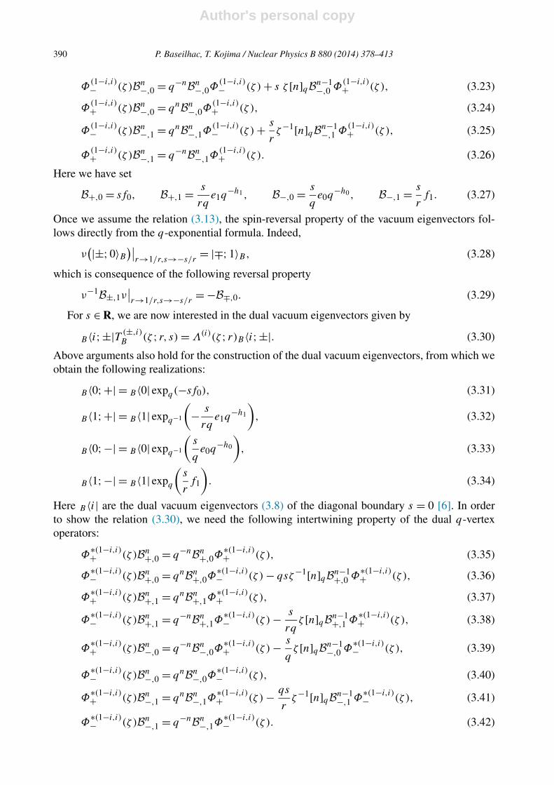
where |i〉B are the vacuum eigenvectors (3.7) of the diagonal boundary s = 0 [6]. Here we haveused the q-exponential function expq(x) given in (1.5). In order to show the relation (3.14), thefollowing intertwining property of the q-vertex operators are needed:
Φ(1−i,i)− (ζ )Bn
+,0 = q−nBn+,0Φ
(1−i,i)− (ζ ), (3.19)
Φ(1−i,i)+ (ζ )Bn
+,0 = qnBn+,0Φ
(1−i,i)+ (ζ ) + s ζ−1[n]qBn−1
+,0 Φ(1−i,i)− (ζ ), (3.20)
Φ(1−i,i)− (ζ )Bn
+,1 = qnBn+,1Φ
(1−i,i)− (ζ ), (3.21)
Φ(1−i,i)+ (ζ )Bn
+,1 = q−nBn+,1Φ
(1−i,i)+ (ζ ) + s
rζ [n]qBn−1
+,1 Φ(1−i,i)− (ζ ), (3.22)
Author's personal copy
390 P. Baseilhac, T. Kojima / Nuclear Physics B 880 (2014) 378–413
Φ(1−i,i)− (ζ )Bn
−,0 = q−nBn−,0Φ
(1−i,i)− (ζ ) + s ζ [n]qBn−1
−,0 Φ(1−i,i)+ (ζ ), (3.23)
Φ(1−i,i)+ (ζ )Bn
−,0 = qnBn−,0Φ
(1−i,i)+ (ζ ), (3.24)
Φ(1−i,i)− (ζ )Bn
−,1 = qnBn−,1Φ
(1−i,i)− (ζ ) + s
rζ−1[n]qBn−1
−,1 Φ(1−i,i)+ (ζ ), (3.25)
Φ(1−i,i)+ (ζ )Bn
−,1 = q−nBn−,1Φ
(1−i,i)+ (ζ ). (3.26)
Here we have set
B+,0 = sf0, B+,1 = s
rqe1q
−h1, B−,0 = s
qe0q
−h0, B−,1 = s
rf1. (3.27)
Once we assume the relation (3.13), the spin-reversal property of the vacuum eigenvectors fol-lows directly from the q-exponential formula. Indeed,
ν(|±;0〉B
)∣∣r→1/r,s→−s/r
= |∓;1〉B, (3.28)
which is consequence of the following reversal property
ν−1B±,1ν∣∣r→1/r,s→−s/r
= −B∓,0. (3.29)
For s ∈ R, we are now interested in the dual vacuum eigenvectors given by
B〈i;±|T (±,i)B (ζ ; r, s) = Λ(i)(ζ ; r)B〈i;±|. (3.30)
Above arguments also hold for the construction of the dual vacuum eigenvectors, from which weobtain the following realizations:
B〈0;+| = B〈0| expq(−sf0), (3.31)
B〈1;+| = B〈1| expq−1
(− s
rqe1q
−h1
), (3.32)
B〈0;−| = B〈0| expq−1
(s
qe0q
−h0
), (3.33)
B〈1;−| = B〈1| expq
(s
rf1
). (3.34)
Here B 〈i| are the dual vacuum eigenvectors (3.8) of the diagonal boundary s = 0 [6]. In orderto show the relation (3.30), we need the following intertwining property of the dual q-vertexoperators:
Φ∗(1−i,i)+ (ζ )Bn
+,0 = q−nBn+,0Φ
∗(1−i,i)+ (ζ ), (3.35)
Φ∗(1−i,i)− (ζ )Bn
+,0 = qnBn+,0Φ
∗(1−i,i)− (ζ ) − qsζ−1[n]qBn−1
+,0 Φ∗(1−i,i)+ (ζ ), (3.36)
Φ∗(1−i,i)+ (ζ )Bn
+,1 = qnBn+,1Φ
∗(1−i,i)+ (ζ ), (3.37)
Φ∗(1−i,i)− (ζ )Bn
+,1 = q−nBn+,1Φ
∗(1−i,i)− (ζ ) − s
rqζ [n]qBn−1
+,1 Φ∗(1−i,i)+ (ζ ), (3.38)
Φ∗(1−i,i)+ (ζ )Bn
−,0 = q−nBn−,0Φ
∗(1−i,i)+ (ζ ) − s
qζ [n]qBn−1
−,0 Φ∗(1−i,i)− (ζ ), (3.39)
Φ∗(1−i,i)− (ζ )Bn
−,0 = qnBn−,0Φ
∗(1−i,i)− (ζ ), (3.40)
Φ∗(1−i,i)+ (ζ )Bn
−,1 = qnBn−,1Φ
∗(1−i,i)+ (ζ ) − qs
rζ−1[n]qBn−1
−,1 Φ∗(1−i,i)− (ζ ), (3.41)
Φ∗(1−i,i)− (ζ )Bn
−,1 = q−nBn−,1Φ
∗(1−i,i)− (ζ ). (3.42)

Author's personal copy
P. Baseilhac, T. Kojima / Nuclear Physics B 880 (2014) 378–413 391
Once we assume the relation (3.13), the spin-reversal property of the dual vacuum eigenvectorsfor a triangular boundary condition follows directly from the q-exponential formula:
ν(B〈0;±|)∣∣
r→1/r,s→−s/r= B〈1;∓|. (3.43)
Finally, from the relation for the q-exponential function expq(x) expq−1(−x) = 1 we deduce
B〈i;±|±; i〉B = B〈i|i〉B. (3.44)
Hence we have
B〈i;±|±; i〉B =⎧⎨⎩
(q4r2;q8)∞(q6;q8)∞(q2r2;q8)∞
(i = 0),
(q4/r2;q8)∞(q6;q8)∞(q2/r2;q8)∞
(i = 1).(3.45)
Here we have used the formulae of the norms of B 〈i|i〉B given in [6].
4. Correlation functions
In this section, two integral representations for correlation functions of q-vertex operatorsare proposed. In particular, it is shown that the expressions obtained for a subset of correlationfunctions for the triangular boundary case coincide with the ones associated with a diagonalboundary. Based on the exact relation between local spin operators and q-vertex operators [3,6],summation formulae for the boundary expectation value of the spin operator in the models (1.1)are derived. In the last subsection, using the spin-reversal property we deduce linear relationsbetween certain multiple integrals involving elliptic theta functions. The simplest examples arepresented.
4.1. Definitions
In this section, we focus our attention on the vacuum expectation values of products of theq-vertex operators given by
P (±,i)ε1,ε2,...,εM
(ζ1, ζ2, . . . , ζM ; r, s)
= B〈i;±|Φ(i,1−i)ε1 (ζ1)Φ
(1−i,i)ε2 (ζ2) · · ·Φ(1−i,i)
εM(ζM)|±; i〉B
B〈i;±|±; i〉B , (4.1)
with M an even integer. Our purpose is to derive them as integrals of meromorphic functionsinvolving infinite products (4.27) and (4.40), which will be detailed in the next two subsections.In particular, as we will show in the next section, upon the condition
∑Mj=1 εj = 0, the vacuum
expectation value of triangular boundary coincides with the one of diagonal boundary. Namely,
B〈i;±|Φ(i,1−i)ε1 (ζ1) · · ·Φ(1−i,i)
εM(ζM)|±; i〉B
B〈i;±|±; i〉B = B〈i|Φ(i,1−i)ε1 (ζ1) · · ·Φ(1−i,i)
εM(ζM)|i〉B
B〈i|i〉B . (4.2)
Note that from the spin-reversal properties (2.34), (3.28), (3.43), we have
P (±,i)ε1,...,εM
(ζ1, . . . , ζM ; r, s) = P(∓,1−i)−ε1,...,−εM
(ζ1, . . . , ζM ;1/r,−s/r), (4.3)
which will be used in the last subsection. We have two bosonizations of the q-vertex operator,which are based on the relation: νΦ
(0,1)ε (ζ )ν = Φ
(1,0)−ε (ζ ). Hence we have two formulae of the
correlation functions in (4.3).
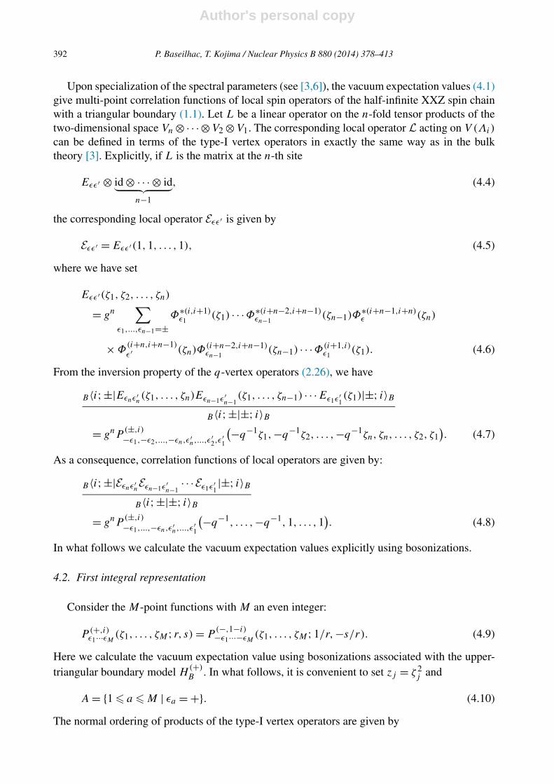
Author's personal copy
392 P. Baseilhac, T. Kojima / Nuclear Physics B 880 (2014) 378–413
Upon specialization of the spectral parameters (see [3,6]), the vacuum expectation values (4.1)give multi-point correlation functions of local spin operators of the half-infinite XXZ spin chainwith a triangular boundary (1.1). Let L be a linear operator on the n-fold tensor products of thetwo-dimensional space Vn ⊗· · ·⊗V2 ⊗V1. The corresponding local operator L acting on V (Λi)
can be defined in terms of the type-I vertex operators in exactly the same way as in the bulktheory [3]. Explicitly, if L is the matrix at the n-th site
Eεε′ ⊗ id ⊗ · · · ⊗ id︸ ︷︷ ︸n−1
, (4.4)
the corresponding local operator Eεε′ is given by
Eεε′ = Eεε′(1,1, . . . ,1), (4.5)
where we have set
Eεε′(ζ1, ζ2, . . . , ζn)
= gn∑
ε1,...,εn−1=±Φ∗(i,i+1)
ε1(ζ1) · · ·Φ∗(i+n−2,i+n−1)
εn−1(ζn−1)Φ
∗(i+n−1,i+n)ε (ζn)
× Φ(i+n,i+n−1)
ε′ (ζn)Φ(i+n−2,i+n−1)εn−1
(ζn−1) · · ·Φ(i+1,i)ε1
(ζ1). (4.6)
From the inversion property of the q-vertex operators (2.26), we have
B〈i;±|Eεnε′n(ζ1, . . . , ζn)Eεn−1ε
′n−1
(ζ1, . . . , ζn−1) · · ·Eε1ε′1(ζ1)|±; i〉B
B〈i;±|±; i〉B= gnP
(±,i)
−ε1,−ε2,...,−εn,ε′n,...,ε′
2,ε′1
(−q−1ζ1,−q−1ζ2, . . . ,−q−1ζn, ζn, . . . , ζ2, ζ1). (4.7)
As a consequence, correlation functions of local operators are given by:
B〈i;±|Eεnε′nEεn−1ε
′n−1
· · ·Eε1ε′1|±; i〉B
B〈i;±|±; i〉B= gnP
(±,i)
−ε1,...,−εn,ε′n,...,ε′
1
(−q−1, . . . ,−q−1,1, . . . ,1). (4.8)
In what follows we calculate the vacuum expectation values explicitly using bosonizations.
4.2. First integral representation
Consider the M-point functions with M an even integer:
P (+,i)ε1···εM
(ζ1, . . . , ζM ; r, s) = P(−,1−i)−ε1···−εM
(ζ1, . . . , ζM ;1/r,−s/r). (4.9)
Here we calculate the vacuum expectation value using bosonizations associated with the upper-triangular boundary model H
(+)B . In what follows, it is convenient to set zj = ζ 2
j and
A = {1 � a � M | εa = +}. (4.10)
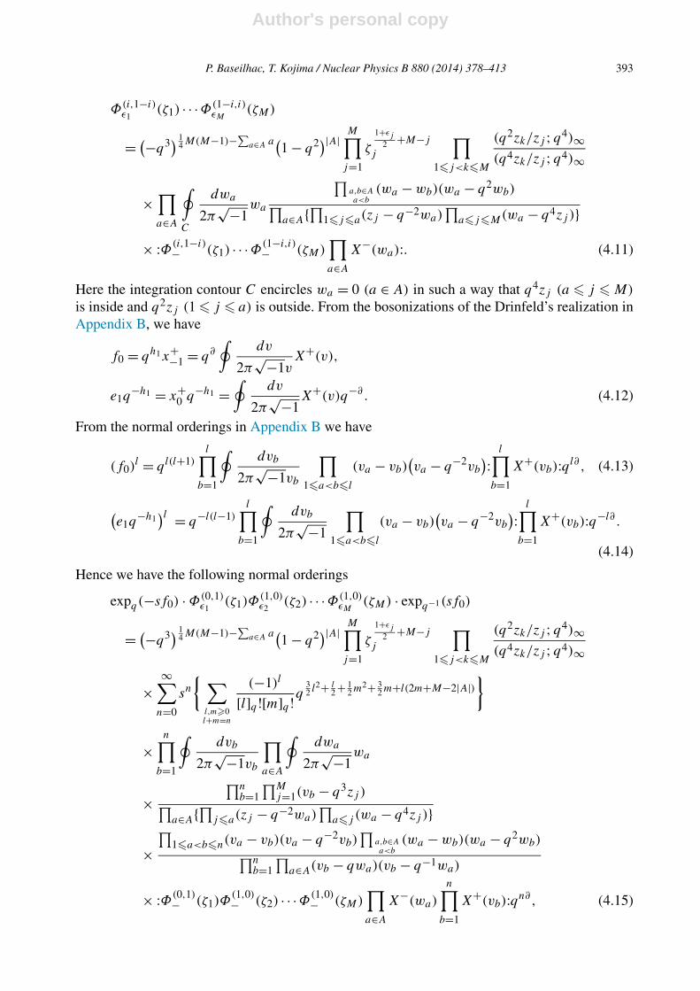
The normal ordering of products of the type-I vertex operators are given by
Author's personal copy
P. Baseilhac, T. Kojima / Nuclear Physics B 880 (2014) 378–413 393
Φ(i,1−i)ε1
(ζ1) · · ·Φ(1−i,i)εM
(ζM)
= (−q3) 14 M(M−1)−∑
a∈A a(1 − q2)|A|M∏
j=1
ζ
1+εj2 +M−j
j
∏1�j<k�M
(q2zk/zj ;q4)∞(q4zk/zj ;q4)∞
×∏a∈A
∮C
dwa
2π√−1
wa
∏a,b∈Aa<b
(wa − wb)(wa − q2wb)∏a∈A{∏1�j�a(zj − q−2wa)
∏a�j�M(wa − q4zj )}
× :Φ(i,1−i)− (ζ1) · · ·Φ(1−i,i)
− (ζM)∏a∈A
X−(wa):. (4.11)
Here the integration contour C encircles wa = 0 (a ∈ A) in such a way that q4zj (a � j � M)
is inside and q2zj (1 � j � a) is outside. From the bosonizations of the Drinfeld’s realization inAppendix B, we have
f0 = qh1x+−1 = q∂
∮dv
2π√−1v
X+(v),
e1q−h1 = x+
0 q−h1 =∮
dv
2π√−1
X+(v)q−∂ . (4.12)
From the normal orderings in Appendix B we have
(f0)l = ql(l+1)
l∏b=1
∮dvb
2π√−1vb
∏1�a<b�l
(va − vb)(va − q−2vb
): l∏b=1
X+(vb):ql∂ , (4.13)
(e1q
−h1)l = q−l(l−1)
l∏b=1
∮dvb
2π√−1
∏1�a<b�l
(va − vb)(va − q−2vb
): l∏b=1
X+(vb):q−l∂ .
(4.14)
Hence we have the following normal orderings
expq(−sf0) · Φ(0,1)ε1
(ζ1)Φ(1,0)ε2
(ζ2) · · ·Φ(1,0)εM
(ζM) · expq−1(sf0)
= (−q3) 14 M(M−1)−∑
a∈A a(1 − q2)|A| M∏j=1
ζ
1+εj2 +M−j
j
∏1�j<k�M
(q2zk/zj ;q4)∞(q4zk/zj ;q4)∞
×∞∑
n=0
sn
{ ∑l,m�0l+m=n
(−1)l
[l]q ![m]q !q32 l2+ l
2 + 12 m2+ 3
2 m+l(2m+M−2|A|)}
×n∏
b=1
∮dvb
2π√−1vb
∏a∈A
∮dwa
2π√−1
wa
×∏n
b=1∏M
j=1(vb − q3zj )∏a∈A{∏j�a(zj − q−2wa)
∏a�j (wa − q4zj )}
×∏
1�a<b�n(va − vb)(va − q−2vb)∏
a,b∈Aa<b
(wa − wb)(wa − q2wb)∏nb=1
∏a∈A(vb − qwa)(vb − q−1wa)
× :Φ(0,1)− (ζ1)Φ
(1,0)− (ζ2) · · ·Φ(1,0)
− (ζM)∏a∈A
X−(wa)
n∏b=1
X+(vb):qn∂, (4.15)
Author's personal copy
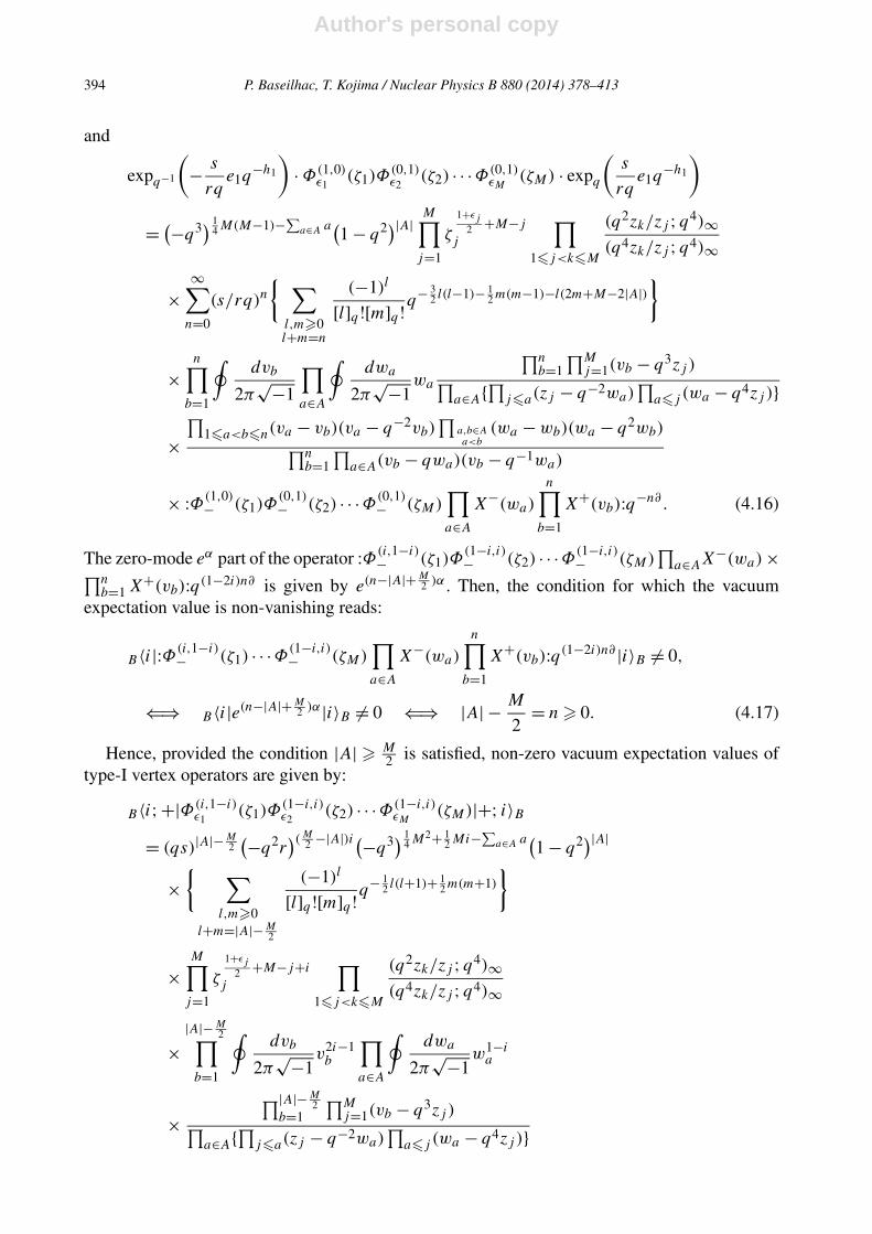
394 P. Baseilhac, T. Kojima / Nuclear Physics B 880 (2014) 378–413
and
expq−1
(− s
rqe1q
−h1
)· Φ(1,0)
ε1(ζ1)Φ
(0,1)ε2
(ζ2) · · ·Φ(0,1)εM
(ζM) · expq
(s
rqe1q
−h1
)= (−q3) 1
4 M(M−1)−∑a∈A a(1 − q2)|A|
M∏j=1
ζ
1+εj2 +M−j
j
∏1�j<k�M
(q2zk/zj ;q4)∞(q4zk/zj ;q4)∞
×∞∑
n=0
(s/rq)n{ ∑
l,m�0l+m=n
(−1)l
[l]q ![m]q !q− 3
2 l(l−1)− 12 m(m−1)−l(2m+M−2|A|)
}
×n∏
b=1
∮dvb
2π√−1
∏a∈A
∮dwa
2π√−1
wa
∏nb=1
∏Mj=1(vb − q3zj )∏
a∈A{∏j�a(zj − q−2wa)∏
a�j (wa − q4zj )}
×∏
1�a<b�n(va − vb)(va − q−2vb)∏
a,b∈Aa<b
(wa − wb)(wa − q2wb)∏nb=1
∏a∈A(vb − qwa)(vb − q−1wa)
× :Φ(1,0)− (ζ1)Φ
(0,1)− (ζ2) · · ·Φ(0,1)
− (ζM)∏a∈A
X−(wa)
n∏b=1
X+(vb):q−n∂ . (4.16)
The zero-mode eα part of the operator :Φ(i,1−i)− (ζ1)Φ
(1−i,i)− (ζ2) · · ·Φ(1−i,i)
− (ζM)∏
a∈AX−(wa)×∏nb=1 X+(vb):q(1−2i)n∂ is given by e(n−|A|+ M
2 )α . Then, the condition for which the vacuumexpectation value is non-vanishing reads:
B〈i|:Φ(i,1−i)− (ζ1) · · ·Φ(1−i,i)
− (ζM)∏a∈A
X−(wa)
n∏b=1
X+(vb):q(1−2i)n∂ |i〉B �= 0,
⇐⇒ B〈i|e(n−|A|+ M2 )α|i〉B �= 0 ⇐⇒ |A| − M
2= n � 0. (4.17)
Hence, provided the condition |A| � M2 is satisfied, non-zero vacuum expectation values of
type-I vertex operators are given by:
B〈i;+|Φ(i,1−i)ε1
(ζ1)Φ(1−i,i)ε2
(ζ2) · · ·Φ(1−i,i)εM
(ζM)|+; i〉B= (qs)|A|− M
2(−q2r
)( M2 −|A|)i(−q3) 1
4 M2+ 12 Mi−∑
a∈A a(1 − q2)|A|
×{ ∑
l,m�0l+m=|A|− M
2
(−1)l
[l]q ![m]q !q− 1
2 l(l+1)+ 12 m(m+1)
}
×M∏
j=1
ζ
1+εj2 +M−j+i
j
∏1�j<k�M
(q2zk/zj ;q4)∞(q4zk/zj ;q4)∞
×|A|− M
2∏b=1
∮dvb
2π√−1
v2i−1b
∏a∈A
∮dwa
2π√−1
w1−ia
×∏|A|− M
2b=1
∏Mj=1(vb − q3zj )∏
a∈A{∏j�a(zj − q−2wa)∏
a�j (wa − q4zj )}
Author's personal copy
P. Baseilhac, T. Kojima / Nuclear Physics B 880 (2014) 378–413 395
×∏
1�a<b�|A|− M2(va − vb)(va − q−2vb)
∏a,b∈Aa<b
(wa − wb)(wa − q2wb)∏|A|− M2
b=1
∏a∈A(vb − qwa)(vb − q−1wa)
× B〈i|e∑M
j=1 P(zj )+∑a∈A R−(wa)+∑|A|− M
2b=1 R+(vb)
× e∑M
j=1 Q(zj )+∑a∈A S−(wa)+∑|A|− M
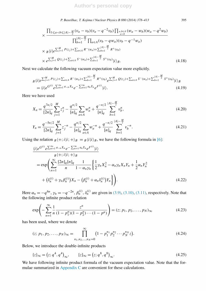
2b=1 S+(vb)|i〉B. (4.18)
Next we calculate the following vacuum expectation value more explicitly.
B〈i|e∑M
j=1 P(zj )+∑a∈A R−(wa)+∑|A|− M
2b=1 R+(vb)e
∑Mj=1 Q(zj )+∑
a∈A S−(wa)+∑|A|− M2
b=1 S+(vb)|i〉B= 〈i|eG(i)
e∑∞
n=1 a−nXne−∑∞n=1 anYneF (i) |i〉. (4.19)
Here we have used
Xn = q7n/2
[2n]qM∑
j=1
znj − qn/2
[n]q∑a∈A
wna + q−n/2
[n]q|A|− M
2∑b=1
vnb , (4.20)
Yn = q−5n/2
[2n]qM∑
j=1
z−nj − qn/2
[n]q∑a∈A
w−na + q−n/2
[n]q|A|− M
2∑b=1
v−nb . (4.21)
Using the relation B 〈+; i|i;+〉B = B 〈i|i〉B , we have the following formula in [6]:
〈i|eG(i)e∑∞
n=1 a−nXne−∑∞n=1 anYneF (i) |i〉
B〈+; i|i;+〉B= exp
( ∞∑n=1
[2n]q [n]qn
1
1 − αnγn
{1
2γnX
2n − αnγnXnYn + 1
2αnY
2n
+ (δ(i)n + γnβ
(i)n
)Xn − (
β(i)n + αnδ
(i)n
)Yn
}). (4.22)
Here αn = −q6n, γn = −q−2n, β(i)n , δ
(i)n are given in (3.9), (3.10), (3.11), respectively. Note that
the following infinite product relation
exp
(−
∞∑n=1
1
n
zn
(1 − pn1 )(1 − pn
2 ) · · · (1 − pn)
)= (z;p1,p2, . . . , pN)∞ (4.23)
has been used, where we denote
(z;p1,p2, . . . , pN)∞ =∞∏
n1,n2,...,nN=0
(1 − p
n11 p
n22 · · ·pnN
N z). (4.24)
Below, we introduce the double-infinite products
{z}∞ = (z;q4, q4)
∞, [z]∞ = (z;q8, q8)
∞. (4.25)
We have following infinite product formula of the vacuum expectation value. Note that the for-mulae summarized in Appendix C are convenient for these calculations.

Author's personal copy
396 P. Baseilhac, T. Kojima / Nuclear Physics B 880 (2014) 378–413
〈i|eG(i)e∑∞
n=1 a−nXne−∑∞n=1 anYneF (i) |i〉
B〈+; i|i;+〉B
=( {q6}∞
{q8}∞)M{(
q4;q2)∞}|A|{(
q2;q2)∞}|A|− M
2
×∏
1�j<k�M
{q6zj zk}∞{q2/zj zk}∞{q6zj /zk}∞{q6zk/zj }∞{q8zj zk}∞{q4/zj zk}∞{q8zj /zk}∞{q8zk/zj }∞
×M∏
j=1
[q10z2j ]∞[q14z2
j ]∞[q10/z2j ]∞[q6/z2
j ]∞[q12z2
j ]∞[q16z2j ]∞[q12/z2
j ]∞[q8/z2j ]∞
×∏M
j=1∏|A|− M
2b=1 (qzj vb;q4)∞(q7zj /vb;q4)∞(qvb/zj ;q4)∞(q3/zj vb;q4)∞∏M
j=1∏
a∈A(q2zjwa;q4)∞(q8zj /wa;q4)∞(q2wa/zj ;q4)∞(q4/zjwa;q4)∞
×∏
a∈A(w2a/q
2;q4)∞(q6/w2a;q4)∞
∏|A|− M2
b=1 (v2b/q
2;q4)∞(q6/v2b;q4)∞∏|A|− M
2b=1
∏a∈A(vbwa/q3;q2)∞(q3vb/wa;q2)∞(q3wa/vb;q2)∞(q5/vbwa;q2)∞
×∏a,b∈Aa<b
(wawb/q
2;q2)∞(q4wa/wb;q2)
∞(q4wb/wa;q2)
∞(q6/wawb;q2)
∞
×∏
1�a<b�|A|− M2
(vavb/q
4;q2)∞(q2va/vb;q2)
∞(q2vb/va;q2)
∞(q4/vavb;q2)
∞
×
⎧⎪⎪⎪⎨⎪⎪⎪⎩∏M
j=1(q2rzj ;q4)∞(q4rzj ;q4)∞
∏|A|− M2
b=1 (1−rvb/q3)∏
a∈A(1−q−2rwa)(i = 0),
∏Mj=1
(1/rzj ;q4)∞(q2/rzj ;q4)∞
∏|A|− M2
b=1 (1−q/rvb)∏a∈A(1−q2/rwa)
(i = 1).
(4.26)
Summarizing the above calculations, we finally obtain the following first integral representationof the M-point functions with M even:
P (+,i)ε1,...,εM
(ζ1, . . . , ζM ; r, s) = P(−,1−i)−ε1,...,−εM
(ζ1, . . . , ζM ;1/r,−s/r)
= (qs)|A|− M2(−q3) 1
4 M2−∑a∈A a
( {q6}∞{q8}∞
)M(q2;q2)2|A|− M
2∞
×∏
1�j<k�M
{q6zj zk}∞{q2/zj zk}∞{q6zj /zk}∞{q2zk/zj }∞{q8zj zk}∞{q4/zj zk}∞{q8zj /zk}∞{q4zk/zj }∞
×M∏
j=1
[q10z2j ]∞[q14z2
j ]∞[q10/z2j ]∞[q6/z2
j ]∞[q12z2
j ]∞[q16z2j ]∞[q12/z2
j ]∞[q8/z2j ]∞
×M∏
j=1
ζ
1+εj2 +M−j
j
∑l,m�0l+m=|A|− M
2
(−1)lq− 12 l(l+1)+ 1
2 m(m+1)
[l]q ![m]q !
Author's personal copy
P. Baseilhac, T. Kojima / Nuclear Physics B 880 (2014) 378–413 397
×∮
· · ·∮
C(+,i)l
∏a∈A
dwa
2π√−1
w1−ia
|A|− M2∏
b=1
dvb
2π√−1
v2i−1b
×∏|A|− M
2b=1
∏Mj=1(vb − q3zj )∏
a∈A{∏1�j�a(zj − q−2wa)∏
a�j�M(wa − q4zj )}
×∏M
j=1∏|A|− M
2b=1 (qzj vb;q4)∞(q7zj /vb;q4)∞(qvb/zj ;q4)∞(q3/zj vb;q4)∞∏M
j=1∏
a∈A(q2zjwa;q4)∞(q8zj /wa;q4)∞(q2wa/zj ;q4)∞(q4/zjwa;q4)∞
×∏
a∈A(w2a/q
2;q4)∞(q6/w2a;q4)∞
∏|A|− M2
b=1 (v2b/q
2;q4)∞(q6/v2b;q4)∞∏|A|− M
2b=1
∏a∈A v2
b(vbwa/q3;q2)∞(q3vb/wa;q2)∞(wa/qvb;q2)∞(q5/vbwa;q2)∞×
∏a,b∈Aa<b
w2a
(wawb/q
2;q2)∞(q4wa/wb;q2)
∞(wb/wa;q2)
∞(q6/wawb;q2)
∞
×∏
1�a<b�|A|− M2
v2a
(vavb/q
4;q2)∞(q2va/vb;q2)
∞(q−2vb/va;q2)
∞(q4/vavb;q2)
∞
×
⎧⎪⎪⎪⎨⎪⎪⎪⎩∏M
j=1(q2rzj ;q4)∞(q4rzj ;q4)∞
∏|A|− M2
b=1 (1−rvb/q3)∏
a∈A(1−q−2rwa)(i = 0),
(−q2r)M2 −|A|(−q3)
M2∏M
j=1 ζj(1/rzj ;q4)∞(q2/rzj ;q4)∞
∏|A|− M2
b=1 (1−q/rvb)∏a∈A(1−q2/rwa)
(i = 1).
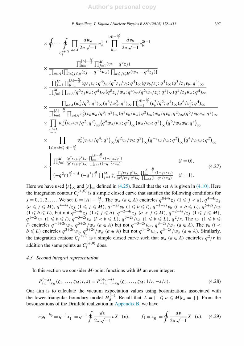
(4.27)
Here we have used {z}∞ and [z]∞ defined in (4.25). Recall that the set A is given in (4.10). Herethe integration contour C
(+,0)l is a simple closed curve that satisfies the following conditions for
s = 0,1,2, . . . . We set L = |A| − M2 . The wa (a ∈ A) encircles q8+4szj (1 � j < a), q4+4szj
(a � j � M), q4+4s/zj (1 � j � M), q3+2svb (1 � b � l), q−1+2svb (l < b � L), q5+2s/vb
(1 � b � L), but not q2−4szj (1 � j � a), q−2−4szj (a < j � M), q−2−4s/zj (1 � j � M),q1−2svb (1 � b � l), q−3−2svb (l < b � L), q3−2s/vb (1 � b � L), q2/r . The vb (1 � b �l) encircles q−1+2swa , q5+2s/wa (a ∈ A) but not q−3−2swa , q3−2s/wa (a ∈ A). The vb (l <
b � L) encircles q3+2swa , q5+2s/wa (a ∈ A) but not q1−2swa , q3−2s/wa (a ∈ A). Similarly,the integration contour C
(+,1)l is a simple closed curve such that wa (a ∈ A) encircles q2/r in
addition the same points as C(+,0)l does.
4.3. Second integral representation
In this section we consider M-point functions with M an even integer:
P (−,i)ε1,...,εM
(ζ1, . . . , ζM ; r, s) = P(+,1−i)−ε1,...,−εM
(ζ1, . . . , ζM ;1/r,−s/r). (4.28)
Our aim is to calculate the vacuum expectation values using bosonizations associated withthe lower-triangular boundary model H
(−)B . Recall that A = {1 � a � M|εa = +}. From the
bosonizations of the Drinfeld realization in Appendix B, we have
e0q−h0 = q−1x−
1 = q−1∮
dv
2π√−1
vX−(v), f1 = x−0 =
∮dv
2π√−1
X−(v). (4.29)
Author's personal copy
398 P. Baseilhac, T. Kojima / Nuclear Physics B 880 (2014) 378–413
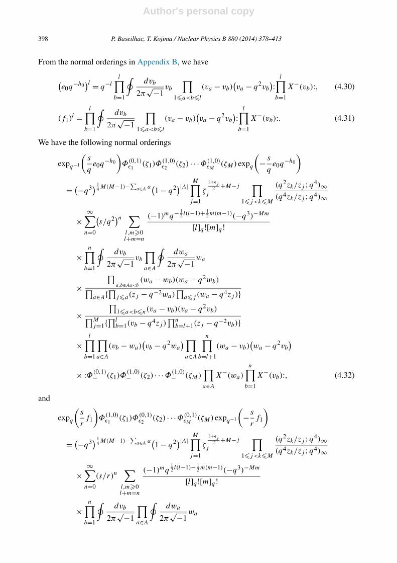
From the normal orderings in Appendix B, we have
(e0q
−h0)l = q−l
l∏b=1
∮dvb
2π√−1
vb
∏1�a<b�l
(va − vb)(va − q2vb
): l∏b=1
X−(vb):, (4.30)
(f1)l =
l∏b=1
∮dvb
2π√−1
∏1�a<b�l
(va − vb)(va − q2vb
): l∏b=1
X−(vb):. (4.31)
We have the following normal orderings
expq−1
(s
qe0q
−h0
)Φ(0,1)
ε1(ζ1)Φ
(1,0)ε2
(ζ2) · · ·Φ(1,0)εM
(ζM) expq
(− s
qe0q
−h0
)
= (−q3) 14 M(M−1)−∑
a∈A a(1 − q2)|A| M∏j=1
ζ
1+εj2 +M−j
j
∏1�j<k�M
(q2zk/zj ;q4)∞(q4zk/zj ;q4)∞
×∞∑
n=0
(s/q2)n ∑
l,m�0l+m=n
(−1)mq− 12 l(l−1)+ 1
2 m(m−1)(−q3)−Mm
[l]q ![m]q !
×n∏
b=1
∮dvb
2π√−1
vb
∏a∈A
∮dwa
2π√−1
wa
×∏
a,b∈Aa<b(wa − wb)(wa − q2wb)∏
a∈A{∏j�a(zj − q−2wa)∏
a�j (wa − q4zj )}
×∏
1�a<b�n(va − vb)(va − q2vb)∏Mj=1{
∏lb=1(vb − q4zj )
∏nb=l+1(zj − q−2vb)}
×l∏
b=1
∏a∈A
(vb − wa)(vb − q2wa
) ∏a∈A
n∏b=l+1
(wa − vb)(wa − q2vb
)× :Φ(0,1)
− (ζ1)Φ(1,0)− (ζ2) · · ·Φ(1,0)
− (ζM)∏a∈A
X−(wa)
n∏b=1
X−(vb):, (4.32)
and
expq
(s
rf1
)Φ(1,0)
ε1(ζ1)Φ
(0,1)ε2
(ζ2) · · ·Φ(0,1)εM
(ζM) expq−1
(− s
rf1
)
= (−q3) 14 M(M−1)−∑
a∈A a(1 − q2)|A| M∏j=1
ζ
1+εj2 +M−j
j
∏1�j<k�M
(q2zk/zj ;q4)∞(q4zk/zj ;q4)∞
×∞∑
n=0
(s/r)n∑
l,m�0l+m=n
(−1)mq12 l(l−1)− 1
2 m(m−1)(−q3)−Mm
[l]q ![m]q !
×n∏
b=1
∮dvb
2π√−1
∏a∈A
∮dwa
2π√−1
wa
Author's personal copy
P. Baseilhac, T. Kojima / Nuclear Physics B 880 (2014) 378–413 399
×∏
a,b∈Aa<b
(wa − wb)(wa − q2wb)∏a∈A{∏j�a(zj − q−2wa)
∏a�j (wa − q4zj )}
×∏
1�a<b�n(va − vb)(va − q2vb)∏Mj=1{
∏lb=1(vb − q4zj )
∏nb=l+1(zj − q−2vb)}
×l∏
a=1
∏b∈A
(va − wb)(va − q2wb
) ∏a∈A
n∏b=l+1
(wa − vb)(wa − q2vb
)× :Φ(0,1)
− (ζ1)Φ(1,0)− (ζ2) · · ·Φ(1,0)
− (ζM)∏a∈A
X−(wa)
n∏b=1
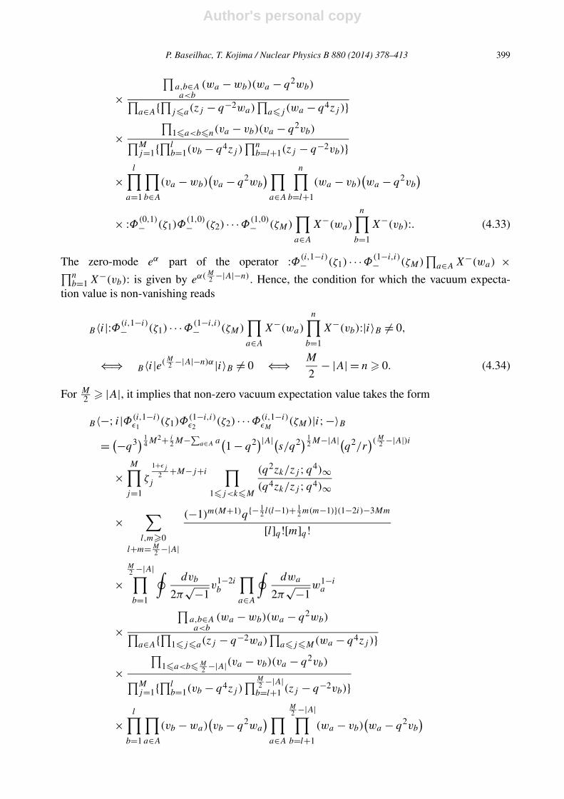
X−(vb):. (4.33)
The zero-mode eα part of the operator :Φ(i,1−i)− (ζ1) · · ·Φ(1−i,i)
− (ζM)∏
a∈A X−(wa) ×∏nb=1 X−(vb): is given by eα( M
2 −|A|−n). Hence, the condition for which the vacuum expecta-tion value is non-vanishing reads
B〈i|:Φ(i,1−i)− (ζ1) · · ·Φ(1−i,i)
− (ζM)∏a∈A
X−(wa)
n∏b=1
X−(vb):|i〉B �= 0,
⇐⇒ B〈i|e( M2 −|A|−n)α|i〉B �= 0 ⇐⇒ M
2− |A| = n � 0. (4.34)
For M2 � |A|, it implies that non-zero vacuum expectation value takes the form
B〈−; i|Φ(i,1−i)ε1
(ζ1)Φ(1−i,i)ε2
(ζ2) · · ·Φ(i,1−i)εM
(ζM)|i;−〉B= (−q3) 1
4 M2+ i2 M−∑
a∈A a(1 − q2)|A|(s/q2) 1
2 M−|A|(q2/r
)( M2 −|A|)i
×M∏
j=1
ζ
1+εj2 +M−j+i
j
∏1�j<k�M
(q2zk/zj ;q4)∞(q4zk/zj ;q4)∞
×∑
l,m�0l+m= M
2 −|A|
(−1)m(M+1)q{− 12 l(l−1)+ 1
2 m(m−1)}(1−2i)−3Mm
[l]q ![m]q !
×M2 −|A|∏b=1
∮dvb
2π√−1
v1−2ib
∏a∈A
∮dwa
2π√−1
w1−ia
×∏
a,b∈Aa<b
(wa − wb)(wa − q2wb)∏a∈A{∏1�j�a(zj − q−2wa)
∏a�j�M(wa − q4zj )}
×∏
1�a<b� M2 −|A|(va − vb)(va − q2vb)∏M
j=1{∏l
b=1(vb − q4zj )∏M
2 −|A|b=l+1 (zj − q−2vb)}
×l∏
b=1
∏a∈A
(vb − wa)(vb − q2wa
) ∏a∈A
M2 −|A|∏b=l+1
(wa − vb)(wa − q2vb
)
Author's personal copy
400 P. Baseilhac, T. Kojima / Nuclear Physics B 880 (2014) 378–413
× B〈i|e∑M
j=1 P(zj )+∑a∈A R−(wa)+∑M
2 −|A|b=1 R−(vb)
× e∑M
j=1 Q(zj )+∑a∈A S−(wa)+∑M
2 −|A|b=1 S−(vb)|i〉B. (4.35)
Next, we calculate the vacuum expectation value more explicitly.
B〈i|e∑M
j=1 P(zj )+∑a∈A R−(wa)+∑M
2 −|A|a=1 R−(va)
e∑M
j=1 Q(zj )+∑a∈A S−(wa)+∑M
2 −|A|a=1 S−(va)|i〉B
= 〈i|eG(i)
e∑∞
n=1 a−nXne−∑∞n=1 anYneF (i) |i〉. (4.36)
Here we have defined
Xn = q7n/2
[2n]qM∑
j=1
znj − qn/2
[n]q∑a∈A
wna − qn/2
[n]q
M2 −|A|∑b=1
vnb , (4.37)
Yn = q−5n/2
[2n]qM∑
j=1
z−nj − qn/2
[n]q∑a∈A
w−na − qn/2
[n]q
M2 −|A|∑b=1
v−nb . (4.38)
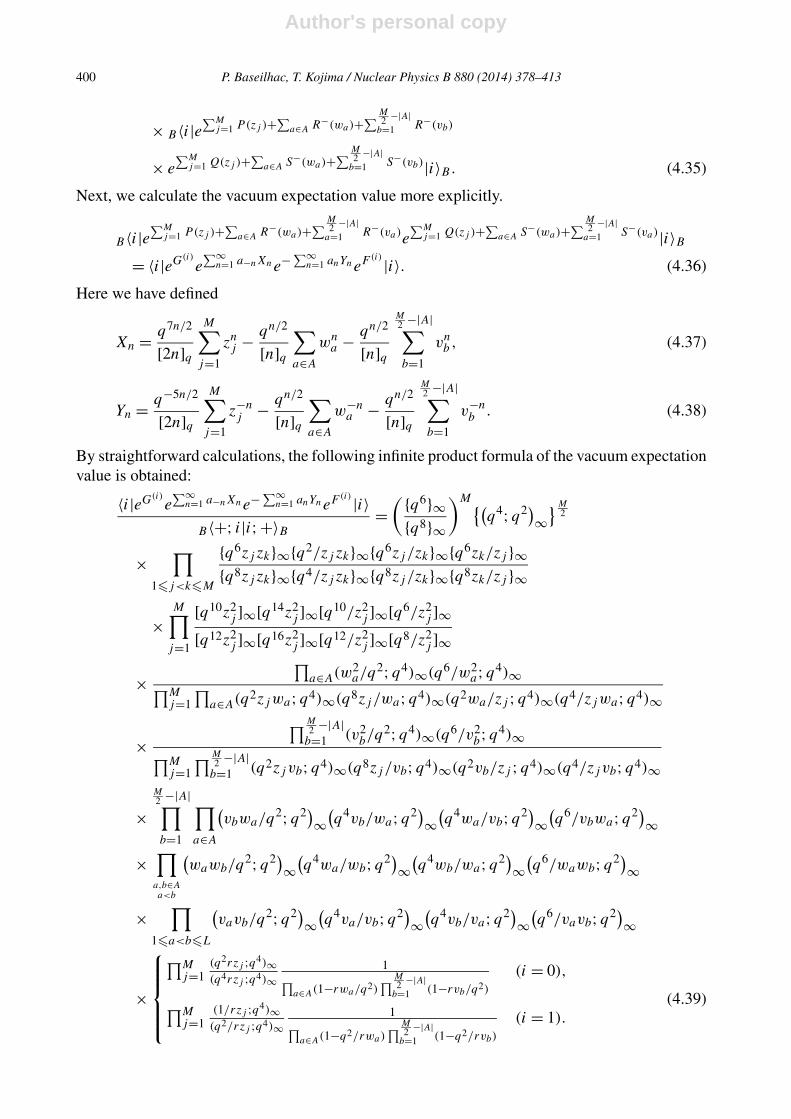
By straightforward calculations, the following infinite product formula of the vacuum expectationvalue is obtained:
〈i|eG(i)e∑∞
n=1 a−nXne−∑∞n=1 anYneF (i) |i〉
B〈+; i|i;+〉B =( {q6}∞
{q8}∞)M{(
q4;q2)∞}M
2
×∏
1�j<k�M
{q6zj zk}∞{q2/zj zk}∞{q6zj /zk}∞{q6zk/zj }∞{q8zj zk}∞{q4/zj zk}∞{q8zj /zk}∞{q8zk/zj }∞
×M∏
j=1
[q10z2j ]∞[q14z2
j ]∞[q10/z2j ]∞[q6/z2
j ]∞[q12z2
j ]∞[q16z2j ]∞[q12/z2
j ]∞[q8/z2j ]∞
×∏
a∈A(w2a/q
2;q4)∞(q6/w2a;q4)∞∏M
j=1∏
a∈A(q2zjwa;q4)∞(q8zj /wa;q4)∞(q2wa/zj ;q4)∞(q4/zjwa;q4)∞
×∏M
2 −|A|b=1 (v2
b/q2;q4)∞(q6/v2
b;q4)∞∏Mj=1
∏M2 −|A|
b=1 (q2zj vb;q4)∞(q8zj /vb;q4)∞(q2vb/zj ;q4)∞(q4/zj vb;q4)∞
×M2 −|A|∏b=1
∏a∈A
(vbwa/q
2;q2)∞(q4vb/wa;q2)
∞(q4wa/vb;q2)
∞(q6/vbwa;q2)
∞
×∏a,b∈Aa<b
(wawb/q
2;q2)∞(q4wa/wb;q2)
∞(q4wb/wa;q2)
∞(q6/wawb;q2)
∞
×∏
1�a<b�L
(vavb/q
2;q2)∞(q4va/vb;q2)
∞(q4vb/va;q2)
∞(q6/vavb;q2)
∞
×
⎧⎪⎪⎪⎨⎪⎪⎪⎩∏M
j=1(q2rzj ;q4)∞(q4rzj ;q4)∞
1∏a∈A(1−rwa/q2)
∏M2 −|A|
b=1 (1−rvb/q2)
(i = 0),
∏Mj=1
(1/rzj ;q4)∞(q2/rzj ;q4)∞
1∏a∈A(1−q2/rwa)
∏M2 −|A|
b=1 (1−q2/rvb)
(i = 1).
(4.39)
Author's personal copy
P. Baseilhac, T. Kojima / Nuclear Physics B 880 (2014) 378–413 401
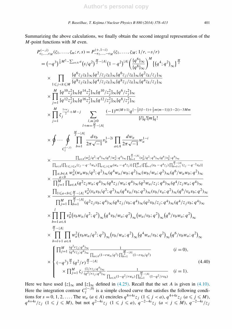
Summarizing the above calculations, we finally obtain the second integral representation of theM-point functions with M even.
P (−,i)ε1,...,εM
(ζ1, . . . , ζm; r, s) = P(+,1−i)−ε1,...,−εM
(ζ1, . . . , ζM ;1/r,−s/r)
= (−q3) 14 M2−∑
a∈A a(s/q2)M
2 −|A|(1 − q2)|A|( {q6}∞
{q8}∞)M{(
q4;q2)∞}M
2
×∏
1�j<k�M
{q6zj zk}∞{q2/zj zk}∞{q6zj /zk}∞{q2zk/zj }∞{q8zj zk}∞{q4/zj zk}∞{q8zj /zk}∞{q4zk/zj }∞
×M∏
j=1
[q10z2j ]∞[q14z2
j ]∞[q10/z2j ]∞[q6/z2
j ]∞[q12z2
j ]∞[q16z2j ]∞[q12/z2
j ]∞[q8/z2j ]∞
×M∏
j=1
ζ
1+εj2 +M−j
j
∑l,m�0
l+m= M2 −|A|
(−1)m(M+1)q{− 12 l(l−1)+ 1
2 m(m−1)}(1−2i)−3Mm
[l]q ![m]q !
×∮
· · ·∮
C(−,i)l
M2 −|A|∏b=1
dvb
2π√−1
v1−2ib
∏a∈A
dwa
2π√−1
w1−ia
×∏
a∈A(w2a/q2;q4)∞(q6/w2
a;q4)∞∏M
2 −|A|b=1 (v2
b/q2;q4)∞(q6/v2b ;q4)∞∏
a∈A{∏1�j�a(zj − q−2wa)∏
a�j�M(wa − q4zj )}∏Mj=1{
∏lb=1(vb − q4zj )
∏M2 −|A|
b=l+1 (zj − q−2vb)}
×∏
a,b∈Aa<b
w2a(wawb/q
2;q2)∞(q4wa/wb;q2)∞(wb/wa;q2)∞(q6/wawb;q2)∞∏Mj=1
∏a∈A(q2zjwa;q4)∞(q8zj /wa;q4)∞(q2wa/zj ;q4)∞(q4/zjwa;q4)∞
×∏
1�a<b� M2 −|A| v
2a(vavb/q
2;q2)∞(q4va/vb;q2)∞(vb/va;q2)∞(q6/vavb;q2)∞∏Mj=1
∏M2 −|A|
b=1 (q2zj vb;q4)∞(q8zj /vb;q4)∞(q2vb/zj ;q4)∞(q4/zj vb;q4)∞
×l∏
b=1
∏a∈A
v2b
(vbwa/q
2;q2)∞(q4vb/wa;q2)
∞(wa/vb;q2)
∞(q6/vbwa;q2)
∞
×M2 −|A|∏b=l+1
∏a∈A
w2a
(vbwa/q
2;q2)∞(vb/wa;q2)
∞(q4wa/vb;q2)
∞(q6/vbwa;q2)
∞
×
⎧⎪⎪⎪⎪⎪⎨⎪⎪⎪⎪⎪⎩
∏Mj=1
(q2rzj ;q4)∞(q4rzj ;q4)∞
1∏a∈A(1−rwa/q2)
∏M2 −|A|
b=1 (1−rvb/q2)
(i = 0),
(−q3)M2 (q2/r)
M2 −|A|
×∏Mj=1 ζj
(1/rzj ;q4)∞(q2/rzj ;q4)∞
1∏a∈A(1−q2/rwa)
∏M2 −|A|
b=1 (1−q2/rvb)
(i = 1).
(4.40)
Here we have used {z}∞ and [z]∞ defined in (4.25). Recall that the set A is given in (4.10).Here the integration contour C
(−,0)l is a simple closed curve that satisfies the following condi-
tions for s = 0,1,2, . . . . The wa (a ∈ A) encircles q8+4szj (1 � j < a), q4+4szj (a � j � M),q4+4s/zj (1 � j � M), but not q2−4szj (1 � j � a), q−2−4szj (a < j � M), q−2−4s/zj

Author's personal copy
402 P. Baseilhac, T. Kojima / Nuclear Physics B 880 (2014) 378–413
(1 � j � M), q2/r . The vb (1 � b � l) encircles q4+4szj , q4+4s/zj (1 � j � M), but notq−2−4szj , q−2−4s/zj (1 � j � M), q2/r . The vb (l < b � M
2 −|A|) encircles q8+4szj , q4+4s/zj
(1 � j � M) but not q2−4szj , q−2−4s/zj (1 � j � M), q2/r . The integration contour C(−,1)l is
a simple closed curve such that wa (a ∈ A) encircles q2/r and vb (1 � b � M2 − |A|) encircles
q2/r in addition the same points as C(+,0)l does.
4.4. Diagonal degeneration
The purpose of this subsection is to identify a sufficient condition such that the expressionsfor a triangular boundary condition coincide with those associated with a diagonal boundarycondition. Let us go back to the formula (4.18). We note that
∑Mj=1 εj = 0 ⇔ n = |A| − M
2 = 0.
Upon the specialization n = |A| − M2 = 0, we have
B〈i;±|Φ(i,1−i)ε1
(ζ1) · · ·Φ(1−i,i)εM
(ζM)|±; i〉B= B〈i|Φ(i,1−i)
ε1(ζ1) · · ·Φ(1−i,i)
εM(ζM)|i〉B. (4.41)
The same argument holds for (4.35). We conclude that upon the parity preserving condition
ε1 + ε2 + · · · + εM = 0, (4.42)
we have the same integral representation as the one for the diagonal boundary conditions [6].Here we note that we have revised misprints in (4.8) of [6].
B〈i;±|Φ(i,1−i)ε1 (ζ1) · · ·Φ(1−i,i)
εM(ζM)|±; i〉B
B〈i;±|±; i〉B
= (−q3) 14 M2−∑
a∈A a( {q6}∞
{q8}∞)M(
q2;q2)M2∞
M∏j=1
ζ
1+εj2 −j+M
j
×∏
1�j<k�M
{q6zj zk}∞{q2/zj zk}∞{q6zj /zk}∞{q2zk/zj }∞{q8zj zk}∞{q4/zj zk}∞{q8zj /zk}∞{q4zk/zj }∞
×M∏
j=1
[q10z2j ]∞[q14z2
j ]∞[q10/z2j ]∞[q6/z2
j ]∞[q12z2
j ]∞[q16z2j ]∞[q12/z2
j ]∞[q8/z2j ]∞
× ∏a∈A
∮C
(i)0
dwa
2π√−1
∏a,b∈Aa<b
w2a(q−2wawb;q2)∞(q4wa/wb;q2)∞(wb/wa;q2)∞(q6/wawb;q2)∞∏
a∈A
∏Mj=1(q2zj wa;q4)∞(q8zj /wa;q4)∞(q2wa/zj ;q4)∞(q4/zj wa;q4)∞
×∏
a∈A(q−2w2a;q4)∞(q6/w2
a;q4)∞∏a∈A{∏1�j�a(zj − wa/q2)
∏a�j�M(wa − q4zj )}
×
⎧⎪⎨⎪⎩∏M
j=1(q2rzj ;q4)∞(q4rzj ;q4)∞
∏a∈A
wa
(1−rwa/q2)(for i = 0),
(−q3)M2∏M
j=1 ζj(1/rzj ;q4)∞(q2/rzj ;q4)∞
∏a∈A
1(1−q2/rwa)
(for i = 1).
(4.43)
Here we have used {z}∞ and [z]∞ defined in (4.25). The integration contour C(0)0 is a simple
closed curve that satisfies the following conditions for s = 0,1,2, . . . . The wa (a ∈ A) encircles
Author's personal copy
P. Baseilhac, T. Kojima / Nuclear Physics B 880 (2014) 378–413 403
q8+4szj (1 � j < a), q4+4szj (a � j � M), q4+4s/zj (1 � j � M), but not q2−4szj (1 � j �a), q−2−4szj (a < j � M), q−2−4s/zj (1 � j � M), q2/r . The integration contour C
(1)0 is a
simple closed curve such that wa (a ∈ A) encircles q2/r in addition the same points as C(0)0
does.To conclude, let us mention that according to the zero-mode operators (4.17) and (4.34), we
have
P (±,i)ε1,...,εM
(ζ1, . . . , ζM ; r, s) = 0 for ±(
M
2− |A|
)> 0. (4.44)
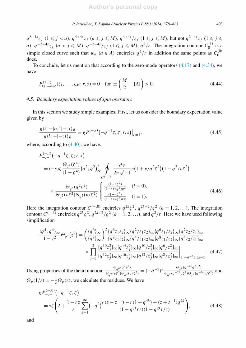
4.5. Boundary expectation values of spin operators
In this section we study simple examples. First, let us consider the boundary expectation valuegiven by
B〈i;−|σ+1 |−; i〉B
B〈i;−|−; i〉B = gP(−,i)−,−
(−q−1ζ, ζ ; r, s)∣∣ζ=1, (4.45)
where, according to (4.40), we have:
P(−,i)−,−
(−q−1ζ, ζ ; r, s)= (−s)ζ
Θq4(ζ 4)
(1 − ζ 4)
(q2;q2)3
∞∮
C(−,i)
dv
2π√−1
v(1 + v/q2ζ 2)(1 − q2/vζ 2)
× Θq4(q2v2)
Θq2(vζ 2)Θq2(v/ζ 2)
⎧⎨⎩(1−rζ 2)
(1−rv/q2)q2 (i = 0),
(1−rζ 2)
(1−rv/q2)rv(i = 1).
(4.46)
Here the integration contour C(−,0) encircles q2kζ 2, q2k+2/ζ 2 (k = 1,2, . . .). The integrationcontour C(−,1) encircles q2kζ 2, q2k+2/ζ 2 (k = 1,2, . . .), and q2/r . Here we have used followingsimplification
(q4;q4)∞1 − z2
Θq4
(z2) =
( {q6}∞{q8}∞
)2 {q6z1z2}∞{q2/z1z2}∞{q6z1/z2}∞{q2z2/z1}∞{q8z1z2}∞{q4/z1z2}∞{q8z1/z2}∞{q4z2/z1}∞
×2∏
j=1
[q10z2j ]∞[q14z2
j ]∞[q10/z2j ]∞[q6/z2
j ]∞[q12z2
j ]∞[q16z2j ]∞[q12/z2
j ]∞[q8/z2j ]∞
∣∣∣∣z1=q−2z,z2=z
. (4.47)
Using properties of the theta function:Θ
q4 (q2v2)
Θq2 (vζ 2)Θ
q2 (v/ζ 2)= (−q−2)k
Θq4 (q−4kq2v2)
Θq2 (q−2kvζ 2)Θ
q2 (q−2kv/ζ 2)and
Θp(1/z) = − 1zΘp(z), we calculate the residues. We have
gP(−,0)−,−
(−q−1ζ, ζ)
= sζ
(2 + 1 − rz
z
∞∑k=1
(−q2)k (z − z−1) − r(1 + q4k) + (z + z−1)q2k
(1 − q2krz)(1 − q2kr/z)
), (4.48)
and
Author's personal copy
404 P. Baseilhac, T. Kojima / Nuclear Physics B 880 (2014) 378–413
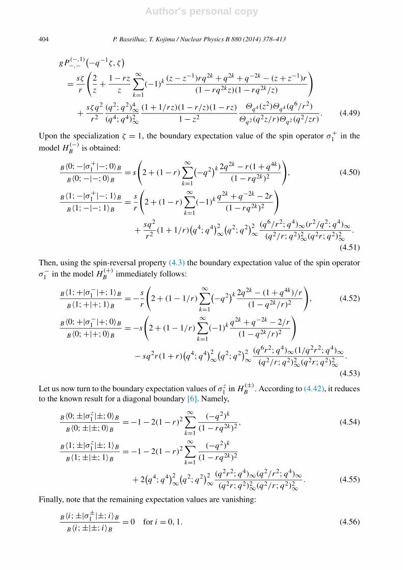
gP(−,1)−,−
(−q−1ζ, ζ)
= sζ
r
(2
z+ 1 − rz
z
∞∑k=1
(−1)k(z − z−1)rq2k + q2k + q−2k − (z + z−1)r
(1 − rq2kz)(1 − rq2k/z)
)
+ sζq2
r2
(q2;q2)4∞(q4;q4)2∞
(1 + 1/rz)(1 − r/z)(1 − rz)
1 − z2
Θq4(z2)Θq4(q6/r2)
Θq2(q2z/r)Θq2(q2/zr). (4.49)
Upon the specialization ζ = 1, the boundary expectation value of the spin operator σ+1 in the
model H(−)B is obtained:
B〈0;−|σ+1 |−;0〉B
B〈0;−|−;0〉B = s
(2 + (1 − r)
∞∑k=1
(−q2)k 2q2k − r(1 + q4k)
(1 − rq2k)2
), (4.50)
B〈1;−|σ+1 |−;1〉B
B〈1;−|−;1〉B = s
r
(2 + (1 − r)
∞∑k=1
(−1)kq2k + q−2k − 2r
(1 − rq2k)2
)
+ sq2
r2(1 + 1/r)
(q4;q4)2
∞(q2;q2)2
∞(q6/r2;q4)∞(r2/q2;q4)∞(q2/r;q2)2∞(q2r;q2)2∞
.
(4.51)
Then, using the spin-reversal property (4.3) the boundary expectation value of the spin operatorσ−
1 in the model H(+)B immediately follows:
B〈1;+|σ−1 |+;1〉B
B〈1;+|+;1〉B = − s
r
(2 + (1 − 1/r)
∞∑k=1
(−q2)k 2q2k − (1 + q4k)/r
(1 − q2k/r)2
), (4.52)
B〈0;+|σ−1 |+;0〉B
B〈0;+|+;0〉B = −s
(2 + (1 − 1/r)
∞∑k=1
(−1)kq2k + q−2k − 2/r
(1 − q2k/r)2
)
− sq2r(1 + r)(q4;q4)2
∞(q2;q2)2
∞(q6r2;q4)∞(1/q2r2;q4)∞(q2/r;q2)2∞(q2r;q2)2∞
.
(4.53)
Let us now turn to the boundary expectation values of σz1 in H
(±)B . According to (4.42), it reduces
to the known result for a diagonal boundary [6]. Namely,
B〈0;±|σz1 |±;0〉B
B〈0;±|±;0〉B = −1 − 2(1 − r)2∞∑
k=1
(−q2)k
(1 − rq2k)2, (4.54)
B〈1;±|σz1 |±;1〉B
B〈1;±|±;1〉B = −1 − 2(1 − r)2∞∑
k=1
(−q2)k
(1 − rq2k)2
+ 2(q4;q4)2
∞(q2;q2)2
∞(q2r2;q4)∞(q2/r2;q4)∞(q2r;q2)2∞(q2/r;q2)2∞
. (4.55)
Finally, note that the remaining expectation values are vanishing:
B〈i;±|σ±1 |±; i〉B
B〈i;±|±; i〉B = 0 for i = 0,1. (4.56)

Author's personal copy
P. Baseilhac, T. Kojima / Nuclear Physics B 880 (2014) 378–413 405
Simplifications occur upon the specializations r = ±1,0,∞: such cases correspond to free (Neu-mann) boundary condition r = −1 (h = 0), fixed (Dirichlet) boundary condition r = 1 (h = ∞)
whereas for r = 0,∞ the Hamiltonian enjoys formal Uq(sl2) invariance.
4.6. Relations between multiple integrals
Linear relations between n-fold integrals are known in the mathematical literature [39–41].In the context of conformal field theory, some examples also arise in the calculation of correla-tion functions which contain screening operators. According to the spin-reversal property (4.3),infinitely many relations of this kind can be exhibited based on previous results. Note that ourrelations cannot be reduced to the relations between n-fold integrals of elliptic gamma functionssummarized in [40,41]. Also, note that we understand the RHS of the spin-reversal property (4.3)as an analytic continuation of the parameter r . Here, we focus on the simplest examples: a rela-tion between a triple integral and a single integral that has been computed explicitly in previoussubsection is exhibited in two different cases. First, from
P(+,0)+,+
(−q−1ζ, ζ ; r, s) = P(−,1)−,−
(−q−1ζ, ζ ;1/r,−s/r)
(4.57)
we have the following identity of multiple integrals of the elliptic theta function:
rzq2 (q2;q2)4∞(q4;q4)2∞
(1 + r/z)(1 − 1/rz)(1 − z/r)
1 − z2
Θq4(z2)Θq4(q6r2)
Θq2(q2rz)Θq2(q2r/z)
+ 2 + (1 − z/r)
∞∑k=1
(−1)k(z − z−1)q2k/r + q2k + q−2k − (z + z−1)/r
(1 − q2kz/r)(1 − q2k/rz)
= q2 (q2;q2)8∞(q4;q4)4∞
Θq4(z2)
1 − z2
(−q2
∫ ∫ ∫C
(+,0)0
+∫ ∫ ∫C
(+,0)1
) 3∏a=1
dwa
2π√−1
w1
w2w53
× (1 − rz)(1 − rw3/q3)
∏2a=1(1 − q2/zwa)∏2
a=1(1 − rwa/q2)(1 − q2w1/w2)(1 − q4/w1w2)
× Θq2(w1w2)Θq2(w2/w1)Θq2(zw3/q)Θq2(qw3/z)∏3
a=1 Θq4(w2a/q
2)∏2a=1 Θq2(waz)Θq2(wa/z)Θq2(w3wa/q)Θq2(wa/qw3)
. (4.58)
Here we have set w3 = v. The integration contour C(+,0)0 is a simple closed curve such that the w1
encircles q2+2sz, q4+2s/z, q−1+2sw3, q5+2s/w3, the w2 encircles q4+2sz, q4+2s/z, q−1+2sw3,q5+2s/w3, and the w3 encircles q3+2swa , q5+2s/wa (a = 1,2), for s = 0,1,2, . . . . The integra-tion contour C
(+,1)1 is a simple closed curve such that the w1 encircles q2+2sz, q4+2s/z, q3+2sw3,
q5+2s/w3, the w2 encircles q4+2sz, q4+2s/z, q3+2sw3, q5+2s/w3, and w3 encircles q−1+2swa ,q5+2s/wa (a = 1,2), for s = 0,1,2, . . . .
Secondly, from
P(+,1)+,+
(−q−1ζ, ζ ; r, s) = P(−,0)−,−
(−q−1ζ, ζ ;1/r,−s/r)
(4.59)
we have the following identity:
Author's personal copy
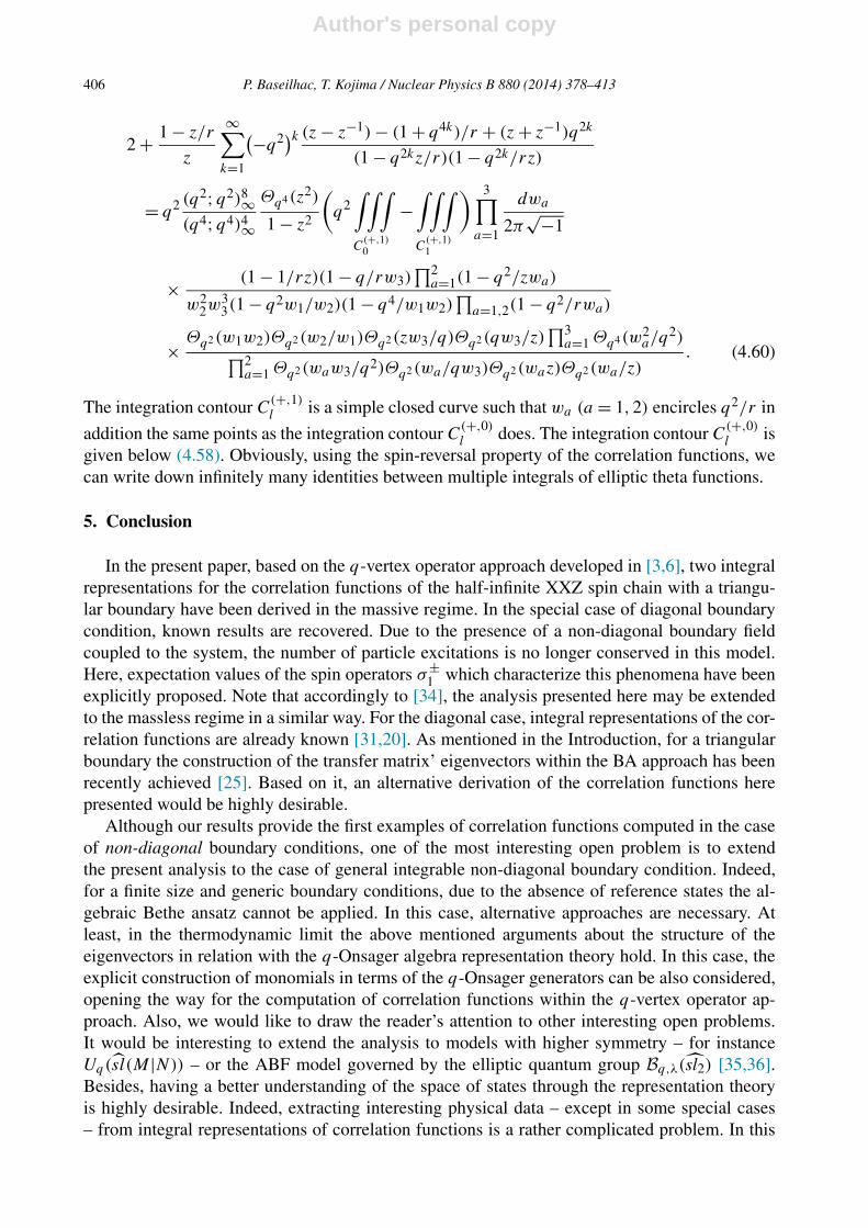
406 P. Baseilhac, T. Kojima / Nuclear Physics B 880 (2014) 378–413
2 + 1 − z/r
z
∞∑k=1
(−q2)k (z − z−1) − (1 + q4k)/r + (z + z−1)q2k
(1 − q2kz/r)(1 − q2k/rz)
= q2 (q2;q2)8∞(q4;q4)4∞
Θq4(z2)
1 − z2
(q2
∫ ∫ ∫C
(+,1)0
−∫ ∫ ∫C
(+,1)1
) 3∏a=1
dwa
2π√−1
× (1 − 1/rz)(1 − q/rw3)∏2
a=1(1 − q2/zwa)
w22w
33(1 − q2w1/w2)(1 − q4/w1w2)
∏a=1,2(1 − q2/rwa)
× Θq2(w1w2)Θq2(w2/w1)Θq2(zw3/q)Θq2(qw3/z)∏3
a=1 Θq4(w2a/q
2)∏2a=1 Θq2(waw3/q2)Θq2(wa/qw3)Θq2(waz)Θq2(wa/z)
. (4.60)
The integration contour C(+,1)l is a simple closed curve such that wa (a = 1,2) encircles q2/r in
addition the same points as the integration contour C(+,0)l does. The integration contour C
(+,0)l is
given below (4.58). Obviously, using the spin-reversal property of the correlation functions, wecan write down infinitely many identities between multiple integrals of elliptic theta functions.
5. Conclusion
In the present paper, based on the q-vertex operator approach developed in [3,6], two integralrepresentations for the correlation functions of the half-infinite XXZ spin chain with a triangu-lar boundary have been derived in the massive regime. In the special case of diagonal boundarycondition, known results are recovered. Due to the presence of a non-diagonal boundary fieldcoupled to the system, the number of particle excitations is no longer conserved in this model.Here, expectation values of the spin operators σ±
1 which characterize this phenomena have beenexplicitly proposed. Note that accordingly to [34], the analysis presented here may be extendedto the massless regime in a similar way. For the diagonal case, integral representations of the cor-relation functions are already known [31,20]. As mentioned in the Introduction, for a triangularboundary the construction of the transfer matrix’ eigenvectors within the BA approach has beenrecently achieved [25]. Based on it, an alternative derivation of the correlation functions herepresented would be highly desirable.
Although our results provide the first examples of correlation functions computed in the caseof non-diagonal boundary conditions, one of the most interesting open problem is to extendthe present analysis to the case of general integrable non-diagonal boundary condition. Indeed,for a finite size and generic boundary conditions, due to the absence of reference states the al-gebraic Bethe ansatz cannot be applied. In this case, alternative approaches are necessary. Atleast, in the thermodynamic limit the above mentioned arguments about the structure of theeigenvectors in relation with the q-Onsager algebra representation theory hold. In this case, theexplicit construction of monomials in terms of the q-Onsager generators can be also considered,opening the way for the computation of correlation functions within the q-vertex operator ap-proach. Also, we would like to draw the reader’s attention to other interesting open problems.It would be interesting to extend the analysis to models with higher symmetry – for instanceUq(sl(M|N)) – or the ABF model governed by the elliptic quantum group Bq,λ(sl2) [35,36].Besides, having a better understanding of the space of states through the representation theoryis highly desirable. Indeed, extracting interesting physical data – except in some special cases– from integral representations of correlation functions is a rather complicated problem. In this
Author's personal copy
P. Baseilhac, T. Kojima / Nuclear Physics B 880 (2014) 378–413 407
direction, the remarkable connection between the q-Onsager algebra and the theory of specialfunctions [42] may be promising, as well as the link between solutions of the reflection quantumKnizhnik–Zamolodchikov equations [43] and Koornwinder polynomials [44,45] (see also [46]).
Finally, we would like to point out that promising routes have been explored recently. WithinSklyanin’s framework, let us mention for instance the functional approach of Galleas [32], theextension of Sklyanin’s separation of variable approach [33] or the modified algebraic Betheansatz approach proposed in [19] which may provide an alternative derivation of above results.
Acknowledgements
The authors would like to thank S. Belliard, V. Fateev, K. Kozlowski, J.M. Maillet, G. Nic-coli, and Y.-Z. Zhang. P.B. thanks J. Stokman for pointing out Ref. [40], and P. Zinn-Justin fordiscussions. T.K. thanks S. Tsujimoto for discussions. T.K. would like to thank Laboratoire deMathématiques et Physique Théorique, Université de Tours, for kind invitation and warm hospi-tality during his stay in March 2013. This work is supported by the Grant-in-Aid for ScientificResearch C (21540228) from JSPS and Visiting professorship from CNRS.
Appendix A. Quantum group Uq(sl2)
In this appendix we recall the definition of Uq(sl2) [47,48] and fix the notation that are usedin the main text. Let −1 < q < 0. Consider a free Abelian group on the letters Λ0,Λ1, δ. We callP = ZΛ0 ⊕ ZΛ1 ⊕ Zδ the weight lattice, Λi the fundamental weights and δ the null root. Definethe simple roots αi (i = 0,1) and the element ρ by α0 +α1 = δ, Λ1 = Λ0 + α1
2 , ρ = Λ0 +Λ1. Let(h0, h1, d) be an ordered basis of P ∗ = Hom(P,Z) dual to (Λ0,Λ1, δ). We define a symmetricbilinear form ( , ) : P × P → 1
2 Z by
(Λ0,Λ0) = 0, (Λ0, α1) = 0, (Λ0, δ) = 1, (α1, α1) = 2,
(α1, δ) = 0, (δ, δ) = 0. (A.1)
Regarding P ∗ ⊂ P via this bilinear form we have the identification
h0 = α0, h1 = α1, d = Λ0. (A.2)
The quantum group Uq(sl2) is a q-analogue of the universal enveloping algebra U(sl2) generatedby Chevalley generators ej , fj (j = 0,1) and qh (h ∈ P ∗) and through the defining relations:
q0 = 1, qhqh′ = qh+h′, (A.3)
qhejq−h = q(h,αj )ej , qhfjq
−h = q−(h,αj )fj , (A.4)
[ei, fj ] = δi,j
qhi − q−hi
q − q−1, (A.5)
e3i ej − [3]qe2
i ej ei + [3]qeiej e2i − ej e
3i = 0 (i �= j), (A.6)
f 3i fj − [3]qf 2
i fj fi + [3]qfifjf2i − fjf
3i = 0 (i �= j). (A.7)
Here we denote:
[n]q = qn − q−n
q − q−1. (A.8)
The quantum group Uq(sl2) has the coproduct Δ structure:

Author's personal copy
408 P. Baseilhac, T. Kojima / Nuclear Physics B 880 (2014) 378–413
Δ(qh
) = qh ⊗ qh, Δ(ej ) = ej ⊗ 1 + qhj ⊗ ej ,
Δ(fj ) = fj ⊗ q−hj + 1 ⊗ fj . (A.9)
The coproduct Δ satisfies an algebra automorphism Δ(XY) = Δ(X)Δ(Y ).The quantum group Uq(sl2) has another realization called the Drinfeld’s second realization.
The generators of the Drinfeld’s realizations are
am (m ∈ Z �=0), x±m (m ∈ Z), γ
12 , K, qd . (A.10)
In order to write down the defining relations, it is convenient to introduce the generating function
X±(z) =∑m∈Z
x±mz−m−1, (A.11)
ψ+(z) = K exp
((q − q−1) ∞∑
n=1
anz−n
), (A.12)
ψ−(z) = K−1 exp
(−(
q − q−1) ∞∑n=1
a−nzn
). (A.13)
Defining relations are given by[γ
12 ,Uq(sl2)
] = 0, (A.14)
[am,an] = δm+n,0[2m]q
m
γ m − γ −m
q − q−1, (A.15)
KamK−1 = am, KX±(z)K−1 = q±2X±(z), (A.16)[am,X±(z)
] = ±[2m]qm
γ ∓|m|/2zmX±(z), (A.17)(z − q±2w
)X±(z)X±(w) = (
q±2z − w)X±(w)X±(z), (A.18)[
X+(z),X−(w)] = 1
(q − q−1)zw
(ψ+(
γ12 w
)δ(z/γw) − ψ−(
γ − 12 w
)δ(γ z/w)
). (A.19)
Here δ(z) = ∑n∈Z zn is a formal power series. Other defining relations are given by
qdγ12 q−d = γ
12 , qdKq−d = K, qdx±
mq−d = qmx±m,
qdamq−d = qmam. (A.20)
The Chevalley generators are related to the Drinfeld generators as follows:
K = qh1, x+0 = e1, x−
0 = f1, γK−1 = qh0,
x−1 = e0q
h1, x+−1 = q−h1f0. (A.21)
The Drinfeld realization is convenient to study bosonizations.
Appendix B. Bosonization
In this appendix we review the bosonizations of the quantum group Uq(sl2) and the q-vertex
operators for level k = 1 [3,9]. The center γ12 of Uq(sl2) satisfies (γ
12 )2 = qh0+h1 = qk on the
Author's personal copy
P. Baseilhac, T. Kojima / Nuclear Physics B 880 (2014) 378–413 409
level k representation. Hence γ = q on the level k = 1 representation. For the level k = 1 case,the defining relation of am (m ∈ Z �=0) (A.15) becomes
[am,an] = δm+n,0[2m]q [m]q
m(m,n �= 0). (B.1)
We introduce the zero-mode operator ∂,α by [∂,α] = 2 and the normal ordering symbol : :
:aman: ={
aman (m < 0),
anam (m > 0),:α∂: = :∂α: = α∂. (B.2)
The bosonization of the irreducible highest representation V (Λi) with fundamental weights Λi
are given by (3.4). On this space the actions of am, eα , ∂ are given by
am
(f ⊗ eβ
) ={
amf ⊗ eβ (m < 0),
[am,f ] ⊗ eβ (m > 0),(B.3)
eα(f ⊗ eβ
) = f ⊗ eα+β, ∂(f ⊗ eβ
) = (α,β)f ⊗ eβ, (B.4)
where f ∈ C[a−1, a−2, . . .], and we have set [∂,Λ0] = 0 and Λ1 = Λ0 + α2 .
The action of other Drinfeld generators is given by
K = q∂, γ = q, (B.5)
X±(z) = exp(R±(z)
)exp
(S±(z)
)e±αz±∂ , (B.6)
qd(1 ⊗ eΛi+nα
) = q−(β,β)/2+i/4(1 ⊗ eΛi+nα), (B.7)
where
R±(z) = ±∞∑
n=1
a−n
[n]q q∓n/2zn, S±(z) = ∓∞∑
n=1
an
[n]q q∓n/2z−n. (B.8)
We have the following bosonizations of the q-vertex operators.
Φ(1−i,i)− (ζ ) = exp
(P(ζ 2)) exp
(Q(ζ 2))eα/2(−q3ζ 2)(∂+i)/2
ζ−i , (B.9)
Φ(1−i,i)+ (ζ ) =
∮C1
dw
2π√−1
(1 − q2)wζ
q(w − q2ζ 2)(w − q4ζ 2):Φ(1−i,i)
− (ζ )X−(w):, (B.10)
Ψ∗(1−i,i)− (ξ) = exp
(−P(q−1ξ2)) exp
(−Q(qξ2))e−α/2(−q3ξ2)(−∂+i)/2
ξ1−i , (B.11)
Ψ∗(1−i,i)+ (ξ) =
∮C2
dw
2π√−1
q2(1 − q2)ξ
(w − q2ξ2)(w − q4ξ2):Ψ ∗(1−i,i)
− (ξ)X+(w):, (B.12)
where
P(z) =∞∑
n=1
a−n
[2n]q q7n/2zn, Q(z) = −∞∑
n=1
an
[2n]q q−5n/2z−n. (B.13)
Here the integration contour C1 is a simple closed curve such that the w encircles q4ζ 2 insidebut not q2ζ 2. The integration contour C2 is a simple closed curve such that the w encircles q2ζ 2
inside but not q4ζ 2.In what follows we summarize normal orderings.
Author's personal copy
410 P. Baseilhac, T. Kojima / Nuclear Physics B 880 (2014) 378–413
Φ(i,1−i)− (ζ1)Φ
(1−i,i)− (ζ2) = (−q3ζ 2
1
) 12(q2ζ 2
2 /ζ 21 ;q4)∞
(q4ζ 22 /ζ 2
1 ;q4)∞:Φ(i,1−i)
− (ζ1)Φ(1−i,i)− (ζ2):, (B.14)
Ψ∗(i,1−i)− (ξ1)Ψ
∗(1−i,i)− (ξ2) = (−q3ξ2
1
) 12
(ξ22 /ξ2
1 ;q4)∞(q2ξ2
2 /ξ21 ;q4)∞
:Ψ ∗(1−i,i)− (ξ1)Ψ
∗(1−i,i)− (ξ2):,
(B.15)
Φ(i,1−i)− (ζ )Ψ
∗(1−i,i)− (ξ) = (−q3ζ 2)− 1
2(q3ξ2/ζ 2;q4)∞(qξ2/ζ 2;q4)∞
:Φ(i,1−i)− (ζ )Ψ
∗(1−i,i)− (ξ):, (B.16)
Ψ∗(i,1−i)− (ξ)Φ
(1−i,i)− (ζ ) = (−q3ξ2)− 1
2(q3ζ 2/ξ2;q4)∞(qζ 2/ξ2;q4)∞
:Ψ ∗(i,1−i)− (ξ)Φ
(1−i,i)− (ζ ):, (B.17)
X+(w1)X+(w2) = w2
1(1 − w2/w1)(1 − w2/q
2w1):X+(w1)X
+(w2):, (B.18)
X−(w1)X−(w2) = w2
1(1 − w2/w1)(1 − q2w2/w1
):X−(w1)X−(w2):, (B.19)
X+(w1)X−(w2) = 1
w21(1 − qw2/w1)(1 − w2/qw1)
:X+(w1)X−(w2):, (B.20)
X−(w1)X+(w2) = 1
w21(1 − qw2/w1)(1 − w2/qw1)
:X−(w1)X+(w2):, (B.21)
Φ(i,1−i)− (ζ )X+(w) = (−q3ζ 2)(1 − w/q3ζ 2):Φ(i,1−i)
− (ζ )X+(w):, (B.22)
X+(w)Φ(i,1−i)− (ζ ) = w
(1 − q3ζ 2/w
):X+(w)Φ(i,1−i)− (ζ ):, (B.23)
Φ(i,1−i)− (ζ )X−(w) = −1
q3ζ 2(1 − w/q2ζ 2):Φ(i,1−i)
− (ζ )X−(w):, (B.24)
X−(w)Φ(i,1−i)− (ζ ) = 1
w(1 − q4ζ 2/w):X−(w)Φ
(i,1−i)− (ζ ):, (B.25)
Ψ∗(i,1−i)− (ξ)X+(w) = −1
q3ξ2(1 − w/q4ξ2):Ψ ∗(i,1−i)
− (ξ)X+(w):, (B.26)
X+(w)Ψ∗(i,1−i)− (ξ) = 1
w(1 − q2ξ2/w):X+(w)Ψ
∗(i,1−i)− (ξ):, (B.27)
Ψ∗(i,1−i)− (ξ)X−(w) = (−q3ξ2)(1 − w/q3ξ2):Ψ ∗(i,1−i)
− (ξ)X−(w):, (B.28)
X−(w)Ψ∗(i,1−i)− (ξ) = w
(1 − q3ξ2/w
):X−(w)Ψ∗(i,1−i)− (ξ):. (B.29)
Appendix C. Convenient formulae
In this appendix we summarize convenient formulae for calculations of vacuum expectationvalues.
exp
( ∞∑n=1
1
(q − q−1)
q(c+2)n
n[2n]q yn
)= (
qc+4y;q4)∞, (C.1)
exp
( ∞∑n=1
1
(q − q−1)
[n]qq(c+2)n
n[2n]2q
yn
)= (qc+5y;q4, q4)∞
(qc+7y;q4, q4)∞, (C.2)
exp
( ∞∑n=1
1
(q − q−1)
q(c+2)n
n[n]q yn
)= (
qc+3y;q4)∞, (C.3)
Author's personal copy
P. Baseilhac, T. Kojima / Nuclear Physics B 880 (2014) 378–413 411
exp
(∑n>0
[n]qn[2n]q
qcn
1 − αnγn
yn
)= (qc+3y;q4, q4)∞
(qc+1y;q4, q4)∞, (C.4)
exp
(∑n>0
[2n]qn[n]q
qcn
1 − αnγn
yn
)= 1
(qc−1y;q2)∞, (C.5)
exp
( ∞∑n=1
[n]qn(1 − αnγn)
δ(i)n qcn/2yn
)=
((qc+3y2;q8, q8)∞(qc+1y2;q8, q8)∞(qc−1y2;q8, q8)∞(qc+5y2;q8, q8)∞
)1/2
×(
(q(c−3)/2+2i r1−2iy;q4, q4)∞(q(c+1)/2+2i r1−2iy;q4, q4)∞
)1−2i
, (C.6)
exp
( ∞∑n=1
[2n]qn(1 − αnγn)
δ(i)n qcn/2yn
)=
((qc−1y2;q8)∞(qc−3y2;q8)∞
)1/2(q(c−5)/2+2i r1−2iy;q4)1−2i
∞ ,
(C.7)
exp
( ∞∑n=1
[n]qn(1 − αnγn)
β(i)n qcn/2yn
)=
((qc+7y2;q8, q8)∞(qc+13y2;q8, q8)∞(qc+9y2;q8, q8)∞(qc+11y2;q8, q8)∞
)1/2
×(
(q(c+9)/2−2i r1−2iy;q4, q4)∞(q(c+13)/2−2i r1−2iy;q4, q4)∞
)1−2i
, (C.8)
exp
( ∞∑n=1
[2n]qn(1 − αnγn)
β(i)n qcn/2yn
)=
((qc+5y2;q8)∞(qc+7y2;q8)∞
)1/2(q(c+7)/2−2i r1−2iy;q4)1−2i
∞ .
(C.9)
References
[1] H.A. Bethe, Zur theorie der metalle I. Eigenfunktionen der linearen atomkette, Z. Phys. 71 (1931) 205–226.[2] R.J. Baxter, Exactly Solved Models in Statistical Mechanics, Academic Press, London, 1982.[3] B. Davies, O. Foda, M. Jimbo, T. Miwa, A. Nakayashiki, Diagonalization of the XXZ Hamiltonian by vertex oper-
ator, Commun. Math. Phys. 151 (1993) 89–153;M. Jimbo, K. Miki, T. Miwa, A. Nakayashiki, Correlation functions of the XXZ model for Δ < −1, Phys. Lett. A168 (1992) 256–263;M. Jimbo, T. Miwa, Algebraic Analysis of Solvable Lattice Model, CBMS Regional Conference Series in Mathe-matics, vol. 85, AMS, 1994.
[4] V.E. Korepin, N.M. Bogoliubov, A.G. Izergin, Quantum Inverse Scattering Method and Correlation Functions,Cambridge Monographs on Mathematical Physics, Cambridge University Press, Cambridge, 1993;A.G. Izergin, V.E. Korepin, The quantum inverse scattering method approach to correlation functions, Commun.Math. Phys. 94 (1984) 67–92;A.G. Izergin, V.E. Korepin, Correlation functions for the Heisenberg XXZ-antiferromagnet, Commun. Math. Phys.99 (1985) 271–302.
[5] N. Kitanine, J.M. Maillet, V. Terras, Form factors of the XXZ Heisenberg spin- 12 finite chain, Nucl. Phys. B 554
(1999) 647–678;N. Kitanine, J.M. Maillet, V. Terras, Correlation functions of the XXZ Heisenberg spin- 1
2 chain in a magnetic field,Nucl. Phys. B 567 (2000) 554–582;J.M. Maillet, V. Terras, On the quantum inverse scattering problem, Nucl. Phys. B 575 (2000) 627–644;N. Kitanine, J.M. Maillet, N.A. Slavnov, V. Terras, Spin–spin correlation functions of the XXZ − 1
2 Heisenbergchain in a magnetic field, Nucl. Phys. B 641 (2002) 487–518.
[6] M. Jimbo, R. Kedem, T. Kojima, H. Konno, T. Miwa, XXZ chain with a boundary, Nucl. Phys. B 441 (1995)437–470.
Author's personal copy
412 P. Baseilhac, T. Kojima / Nuclear Physics B 880 (2014) 378–413
[7] N. Reshetikhin, Calculation of the norm of Bethe vectors in models with SU(3)-symmetry, J. Sov. Math. 46 (1989)1694–1706;M. Gaudin, La fonction d’onde de Bethe, Masson, Paris, 1983;V.E. Korepin, Calculation of norms of Bethe wave functions, Commun. Math. Phys. 86 (1982) 391–418.
[8] M. Wheeler, Multiple integral formulae for the scalar product of on-shell and off-shell Bethe vectors inSU(3)-invariant models, Nucl. Phys. B 875 (2013) 186–212;S. Belliard, S. Pakuliak, E. Ragoucy, N.A. Slavnov, Bethe vectors of quantum integrable models with GL(3) trigono-metric R-matrix, preprint, arXiv:1304.7602, 2013.
[9] I.B. Frenkel, N. Jing, Vertex representations of quantum affine algebras, Proc. Natl. Acad. Sci. USA 85 (1988)9373–9377.
[10] Y. Koyama, Staggered polarization of vertex models with Uq(sl(n))-symmetry, Commun. Math. Phys. 164 (1994)277–291.
[11] N. Jing, S. Kang, Y. Koyama, Vertex operators of quantum affine Lie algebras Uq(D(1)n ), Commun. Math. Phys.
174 (1995) 367–392.
[12] D. Bernard, Vertex operator representations of the quantum affine algebra Uq(B(1)r ), Lett. Math. Phys. 17 (1989)
239–245.[13] K. Kimura, J. Shiraishi, J. Uchiyama, A level-one representation of the quantum affine superalgebra Uq(sl(M + 1|
N + 1)), Commun. Math. Phys. 188 (1997) 367–378;Y.-Z. Zhang, Level-one representations and vertex operators of quantum affine superalgebra Uq(gl(N |N)), J. Math.Phys. 40 (1999) 6110–6124.
[14] E.K. Sklyanin, Boundary conditions for integrable quantum systems, J. Phys. A 21 (1988) 2375–2389.[15] R. Nepomechie, Bethe ansatz solution of the open XXZ chain with nondiagonal boundary terms, Special issue on
recent advances in the theory of quantum integrable systems J. Phys. A 37 (2004) 433–440.[16] J. Cao, H.-Q. Lin, K.-J. Shi, Y. Wang, Exact solution of XXZ spin chain with unparallel boundary fields, Nucl. Phys.
B 663 (2003) 487–519;W.-L. Yang, Y.-Z. Zhang, On the second reference state and complete eigenstates of the open XXZ chain, J. HighEnergy Phys. 0704 (2007) 44 (11 pp.).
[17] R. Murgan, R.I. Nepomechie, C. Shi, Boundary energy of the open XXZ chain from new exact solutions, Ann.Henri Poincaré 7 (2006) 1429–1448.
[18] J. Cao, W.-L. Yang, K. Shi, Y. Wang, Off-diagonal Bethe ansatz solutions of the anisotropic spin-1/2 chains witharbitrary boundary fields, Nucl. Phys. B 877 (2013) 152–175, arXiv:1307.2023.
[19] S. Belliard, N. Crampé Heisenberg, XXX model with general boundaries: Eigenvectors from Algebraic Betheansatz, SIGMA 9 (2013) 072, arXiv:1309.6165.
[20] N. Kitanine, K.K. Kozlowski, J.M. Maillet, G. Niccoli, N.A. Slavnov, V. Terras, Correlation functions of the openXXZ chain. I, J. Stat. Mech. (2007) P10009 (37 pp.);N. Kitanine, K.K. Kozlowski, J.M. Maillet, G. Niccoli, N.A. Slavnov, V. Terras, Correlation functions of the openXXZ chain. II, J. Stat. Mech. (2008) P07010 (33 pp.).
[21] H. Furutsu, T. Kojima, The Uq(sln) analogue of the XXZ chain with a boundary, J. Math. Phys. 41 (2000)4413–4436.
[22] W.-L. Yang, Y.-Z. Zhang, Izergin–Korepin model with a boundary, Nucl. Phys. B 596 (2001) 495–512;T. Kojima, A remark on ground state of boundary Izergin–Korepin model, Int. J. Mod. Phys. A 26 (2011)1973–1989.
[23] T. Kojima, Diagonalization of transfer matrix of supersymmetry Uq(sl(M + 1|N + 1)) chain with a boundary,J. Math. Phys. 54 (2013) 043507 (40 pp.).
[24] S. Belliard, N. Crampé, E. Ragoucy, Algebraic Bethe ansatz for open XXX model with triangular boundary matrices,Lett. Math. Phys. 103 (2013) 493–506.
[25] R.A. Pimenta, A. Lima-Santos, Algebraic Bethe ansatz for the six vertex model with upper triangular K-matrices,J. Phys. A 46 (2013) 455002, arXiv:1308.4446.
[26] P. Baseilhac, K. Koizumi, A new (in)finite-dimensional algebra for quantum integrable models, Nucl. Phys. B 720(2005) 325–347;P. Baseilhac, K. Koizumi, Exact spectrum of the XXZ open spin chain from the q-Onsager algebra representationtheory, J. Stat. Mech. (2007) P09006 (27 pp.);P. Baseilhac, The q-deformed analogue of the Onsager algebra: beyond the Bethe ansatz approach, Nucl. Phys. B754 (2006) 309–328;P. Baseilhac, K. Shigechi, A new current algebra and the reflection equation, Lett. Math. Phys. 92 (2010) 47–65.
[27] P. Baseilhac, S. Belliard, The half-infinite XXZ chain in Onsager’s approach, Nucl. Phys. B 873 (2013) 550–583.
Author's personal copy
P. Baseilhac, T. Kojima / Nuclear Physics B 880 (2014) 378–413 413
[28] P. Baseilhac, S. Belliard, Central extension of the reflection equations and an analog of Miki’s formula, J. Phys. A44 (2011) 415205, arXiv:1104.1591.
[29] H.J. de Vega, A. Gonza’lez-Ruiz, Boundary K-matrices for the XYZ, XXZ and XXX spin chains, J. Phys. A 27(1994) 6129–6137.
[30] S. Ghoshal, Al. Zamolodchikov, Boundary S matrix and boundary state in two-dimensional integrable quantumfield theory, Int. J. Mod. Phys. A 9 (1994) 3841–3885.
[31] T. Kojima, The massless XXZ chain with a boundary, Int. J. Mod. Phys. A 16 (2001) 409–424.[32] W. Galleas, Functional relations from the Yang–Baxter algebra: Eigenvalues of the XXZ model with non-diagonal
twisted and open boundary conditions, Nucl. Phys. B 790 (2008) 524–542, arXiv:1002.1623.[33] G. Niccoli, Antiperiodic spin- 1
2 XXZ quantum chains by separation of variables: complete spectrum and formfactors, Nucl. Phys. B 870 (2013) 397–420;G. Niccoli, Non-diagonal open spin- 1
2 -XXZ quantum chains by separation of variables: complete spectrum andmatrix elements of some quasi-local operators, J. Stat. Mech. (2012) P10025 (42 pp.).
[34] M. Jimbo, T. Miwa, Quantum KZ equation with |q| = 1 and correlation functions of the XXZ model in the gaplessregime, J. Phys. A 29 (1996) 2923–2958;M. Jimbo, H. Konno, T. Miwa, Massless XXZ model and degeneration of the elliptic algebra Aq,p(sl2), in: Defor-mation Theory and Symplectic Geometry, Ascona, 1996, in: Math. Phys. Stud., vol. 20, Kluwer, Dordrecht, 1997,pp. 117–138.
[35] R.J. Baxter, Variational approximations for square lattice models in statistical mechanics, J. Stat. Phys. 19 (1978)461–478.
[36] T. Miwa, R. Weston, Boundary ABF models, Nucl. Phys. B 486 (1997) 517–545;
T. Kojima, Diagonalization of infinite transfer matrix of boundary Uq,p(A(1)N−1) face model, J. Math. Phys. 52
(2011) 013501 (30 pp.).[37] M. Jimbo, T. Miwa, A. Nakayashiki, Difference equations for the correlation functions of the eight-vertex model,
J. Phys. A 26 (1993) 2199–2209.[38] O. Foda, T. Miwa, Corner transfer matrices and quantum affine algebras, Int. J. Mod. Phys. A 7 (Suppl. 1A) (1992)
279–302.[39] V. Tarasov, A. Varchenko, Identities between q-hypergeometric and hypergeometric integrals of different dimen-
sions, Adv. Math. 191 (2005) 29–45.[40] E.M. Rains, Transformations of elliptic hypergeometric integrals, Ann. Math. 171 (2010) 169–243.[41] V.P. Spiridonov, Theta hypergeometric integrals, Algebra Anal. 15 (2003) 161–215, arXiv:math/0303205v2.[42] P. Terwilliger, in: A.N. Kirillov, A. Tsuchiya, H. Umemura (Eds.), Proceedings of the Nagoya 1999 International
Workshop on Physics and Combinatorics, World Scientific, River Edge, NJ, 2001, pp. 377–398, arXiv:math.QA/0307016.
[43] M. Jimbo, R. Kedem, H. Konno, T. Miwa, R. Weston, Difference equations in spin chains with a boundary, Nucl.Phys. B 448 (1995) 429–456, arXiv:hep-th/9502060.
[44] M. Kasatani, Boundary quantum Knizhnik–Zamolodchikov equation, in: New Trends in Quantum Integrable Sys-tems, World Scientific, Hackensack, NJ, 2011, pp. 157–171.
[45] N. Reshetikhin, J. Stokman, B. Vlaar, Reflection quantum Knizhnik–Zamolodchikov equations and Bethe vectors,arXiv:1305.1113;J. Stokman, B. Vlaar, Koornwinder polynomials and the XXZ spin chain, arXiv:1310.5545.
[46] P. Di Francesco, P. Zinn-Justin, Quantum Knizhnik–Zamolodchikov equation: reflecting boundary conditions andcombinatorics, J. Stat. Mech. Theory Exp. 12 (2007) P12009 (30 pp.), arXiv:0709.3410.
[47] M. Jimbo, A q-difference analogue of U(g) and the Yang–Baxter equation, Lett. Math. Phys. 10 (1985) 63–69.[48] V.G. Drinfeld, A new realization of Yangians and of quantum affine algebras, Sov. Math. Dokl. 36 (1988) 212–216.