A LESSON ON PROBABILITY DISTRIBUTIONS -...
23
An Experiment on Random Variables and Probability Distributions Created by Richard Born Associate Professor Emeritus Northern Illinois University [email protected] Topics Robotics Probability and Statistics Computer Science Ages Junior and Senior High School Students Duration variable from 50 to 90 min O Z O B O T S T R E A M APPROVED
Transcript of A LESSON ON PROBABILITY DISTRIBUTIONS -...

An Experiment on Random Variables and Probability
Distributions
Created by
Richard Born
Associate Professor Emeritus
Northern Illinois University
Topics
Robotics
Probability and Statistics
Computer Science
Ages
Junior and Senior High School Students
Duration
variable from 50 to 90 min
A
PPROVED
OZO
BOT STREA
M
APPROVED

1 © 2015 Richard G. Born
AN EXPERIMENT ON RANDOM VARIABLES AND PROBABILITY DISTRIBUTIONS
TEACHER’S GUIDE
What will students learn?
• What is meant by a random variable and a probability distribution? • What is the probability distribution for the sum of the faces up when
tossing a pair of ordinary dice? How can a pair of Ozobots be used to simulate tossing a pair of ordinary dice?
• What is the probability distribution for the number of tails when tossing three coins? What is the probability distribution for the number of runs when tossing three coins? How can Ozobot be used to simulate tossing three coins?
• What is the probability distribution for the sum of faces-down when tossing an engineer’s ruler that has been marked with the three sides numbered 1, 2, and 3? What is the probability distribution for the absolute value of the difference of faces down? How can Ozobot be used to simulate tossing an engineer’s ruler?
• Give examples of probability distributions that are uniform or triangular. • What characterizes probability distributions that are symmetric?
asymmetric? • How can probability distributions be represented by tables or graphs?
How can the graphs be used to visually compare the probability distributions with experimental results?
• What property of Ozobot makes all of the above simulations possible? • What probability rule is used in all of the above simulations?
Tossing a Pair of Ordinary Dice
If an ordinary six-sided die is thrown, most people find it reasonable to assume that upon stopping, any one face is as likely to be on top as another. Each of the outcomes is equally likely, or equally probable. Each outcome has a “one chance in six” of occurring. We could say that the probability is 1/6 ≈ 0.167, as mathematicians typically describe probabilities by numbers between 0 and 1, with 1 representing absolute certainty that the event will occur.
Probability distributions are used to summarize the probabilities, and can be represented in tabular or graphical form. As an example, the probability

2 © 2015 Richard G. Born
distribution for tossing an ordinary six-sided die is shown below. This distribution is said to be a uniform distribution, as the probabilities of tossing each of the numbers from 1 through 6 is the same, or uniform.
Many board games involve the use of a pair of dice to randomly move a player’s token from space-to-space around the board, based upon the sum of the faces up for the pair of dice thrown. The minimum number of spaces that a player would move is 2, while the maximum number is 12. But what are the probabilities for the sums 2, 3, 4, …, 12?
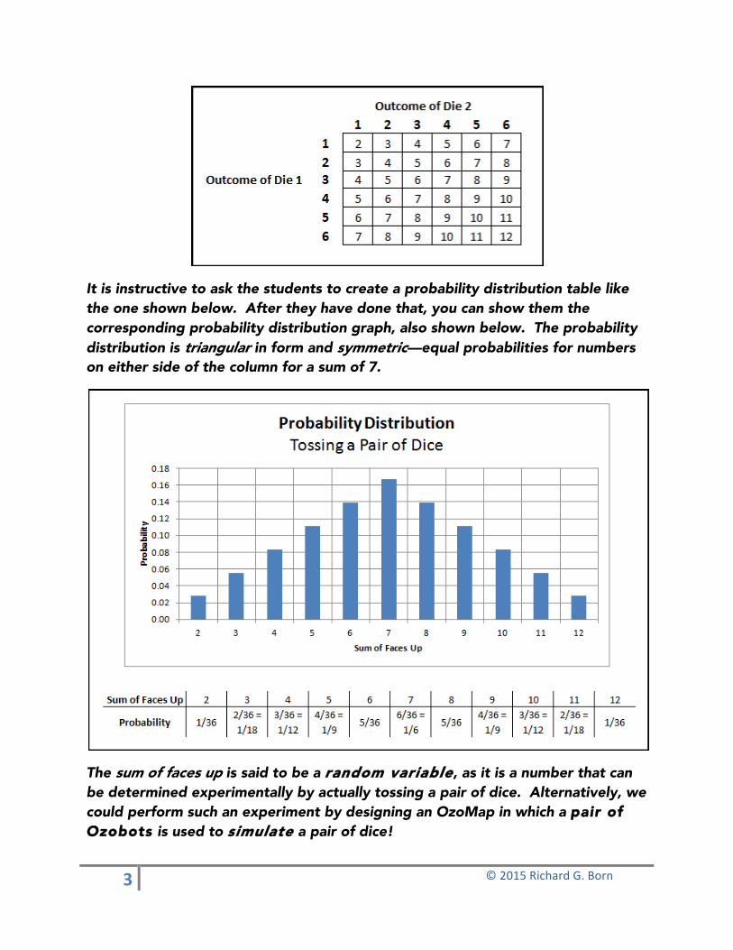
We could represent the set of all equally likely outcomes when tossing a pair of dice in a two-dimensional table like that shown on the next page. The numbers in the grid represent the sum of the faces up after a toss. We notice that there is only 1 way to get a sum of 2—by tossing two 1’s. In contrast, there are 6 ways to get a sum of 7, as shown by the diagonal running from the lower left to the upper right of the grid. You could get a sum of 7 by tossing: (6,1), (5,2), (4,3), (3,4), (2,5), or (1,6), where each ordered pair of numbers represents the outcome of die 1 and die 2, respectively.
3 © 2015 Richard G. Born
It is instructive to ask the students to create a probability distribution table like the one shown below. After they have done that, you can show them the corresponding probability distribution graph, also shown below. The probability distribution is triangular in form and symmetric—equal probabilities for numbers on either side of the column for a sum of 7.
The sum of faces up is said to be a random variable, as it is a number that can be determined experimentally by actually tossing a pair of dice. Alternatively, we could perform such an experiment by designing an OzoMap in which a pair of Ozobots is used to simulate a pair of dice!
4 © 2015 Richard G. Born
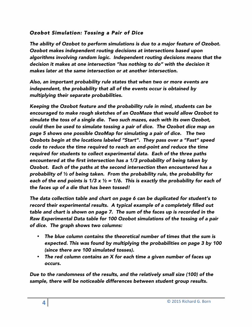
Ozobot Simulation: Tossing a Pair of Dice
The ability of Ozobot to perform simulations is due to a major feature of Ozobot. Ozobot makes independent routing decisions at intersections based upon algorithms involving random logic. Independent routing decisions means that the decision it makes at one intersection “has nothing to do” with the decision it makes later at the same intersection or at another intersection.
Also, an important probability rule states that when two or more events are independent, the probability that all of the events occur is obtained by multiplying their separate probabilities.
Keeping the Ozobot feature and the probability rule in mind, students can be encouraged to make rough sketches of an OzoMaze that would allow Ozobot to simulate the toss of a single die. Two such mazes, each with its own Ozobot, could then be used to simulate tossing a pair of dice. The Ozobot dice map on page 5 shows one possible OzoMap for simulating a pair of dice. The two Ozobots begin at the locations labeled “Start”. They pass over a “Fast” speed code to reduce the time required to reach an end-point and reduce the time required for students to collect experimental data. Each of the three paths encountered at the first intersection has a 1/3 probability of being taken by Ozobot. Each of the paths at the second intersection then encountered has a probability of ½ of being taken. From the probability rule, the probability for each of the end points is 1/3 x ½ = 1/6. This is exactly the probability for each of the faces up of a die that has been tossed!
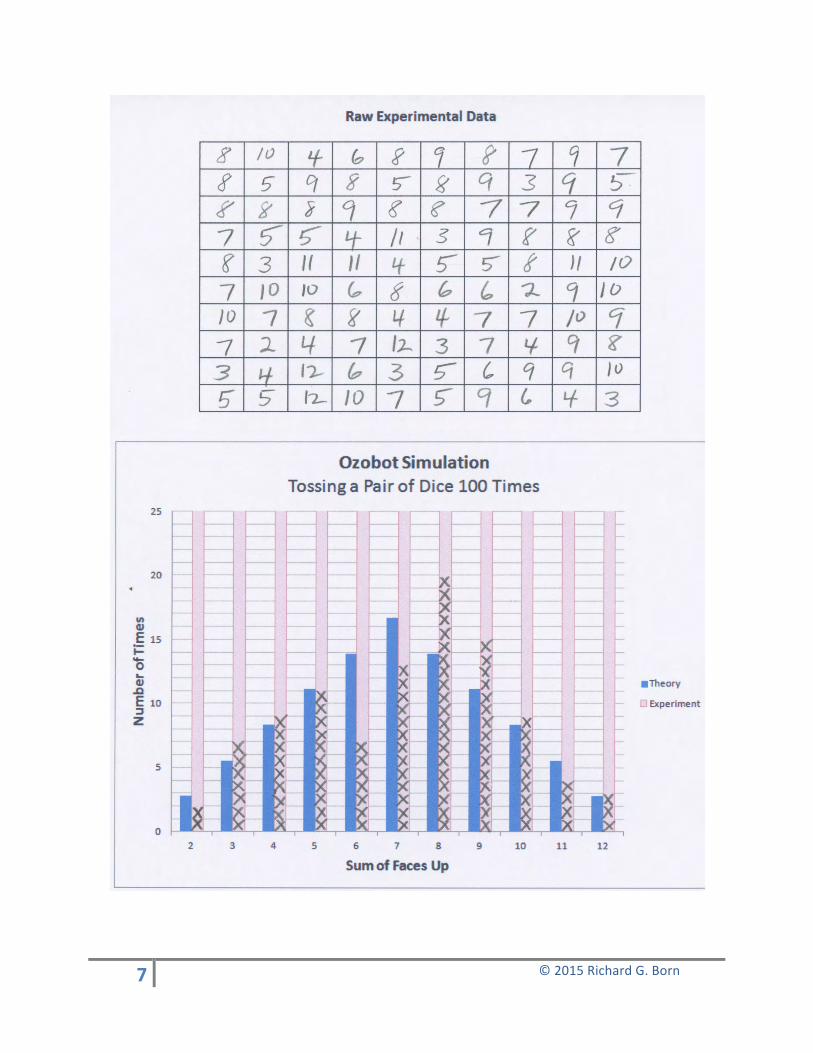
The data collection table and chart on page 6 can be duplicated for student’s to record their experimental results. A typical example of a completely filled out table and chart is shown on page 7. The sum of the faces up is recorded in the Raw Experimental Data table for 100 Ozobot simulations of the tossing of a pair of dice. The graph shows two columns:
• The blue column contains the theoretical number of times that the sum is expected. This was found by multiplying the probabilities on page 3 by 100 (since there are 100 simulated tosses).
• The red column contains an X for each time a given number of faces up occurs.
Due to the randomness of the results, and the relatively small size (100) of the sample, there will be noticeable differences between student group results.

5 © 2015 Richard G. Born

6 © 2015 Richard G. Born
7 © 2015 Richard G. Born

8 © 2015 Richard G. Born
Tossing Three Coins
Every American football game begins with the toss of the coin, with team captains participating in the toss. The coin will land either heads or tails, giving one of the teams the privilege of deciding which team will receive the kickoff or which goal to defend. Most of us will agree that heads and tails are equally probable, each with a probability of ½ = 0.5 when a single coin is tossed.
Things get a bit more interesting when more than one coin is tossed. Suppose that we toss three coins. In this case there are eight equally likely outcomes: HHH, HHT, HTH, HTT, THH, THT, TTH, and TTT, with each triple representing the result of tossing the first, second and third coin, respectively. The probability for any one of these eight equally likely outcomes is 1/8 = 0.125.
Now let’s introduce a random variable into our three-coin game. Suppose that the random variable is the number of tails tossed. If we toss three coins, the result could be 0, 1, 2, or 3 tails. These results are not equally probable. If you study the list of eight equally likely outcomes, you will see that 1 outcome results in 0 tails, 3 result in 1 tail, 3 result in 2 tails, and 1 results in 3 tails. The respective probabilities are 1/8, 3/8, 3/8, and 1/8. The probability distribution for the random variable “number of tails” tossed would then appear as:
9 © 2015 Richard G. Born
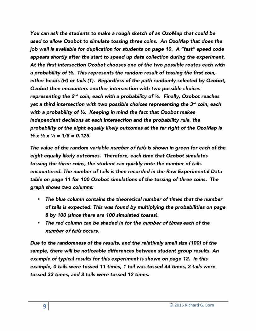
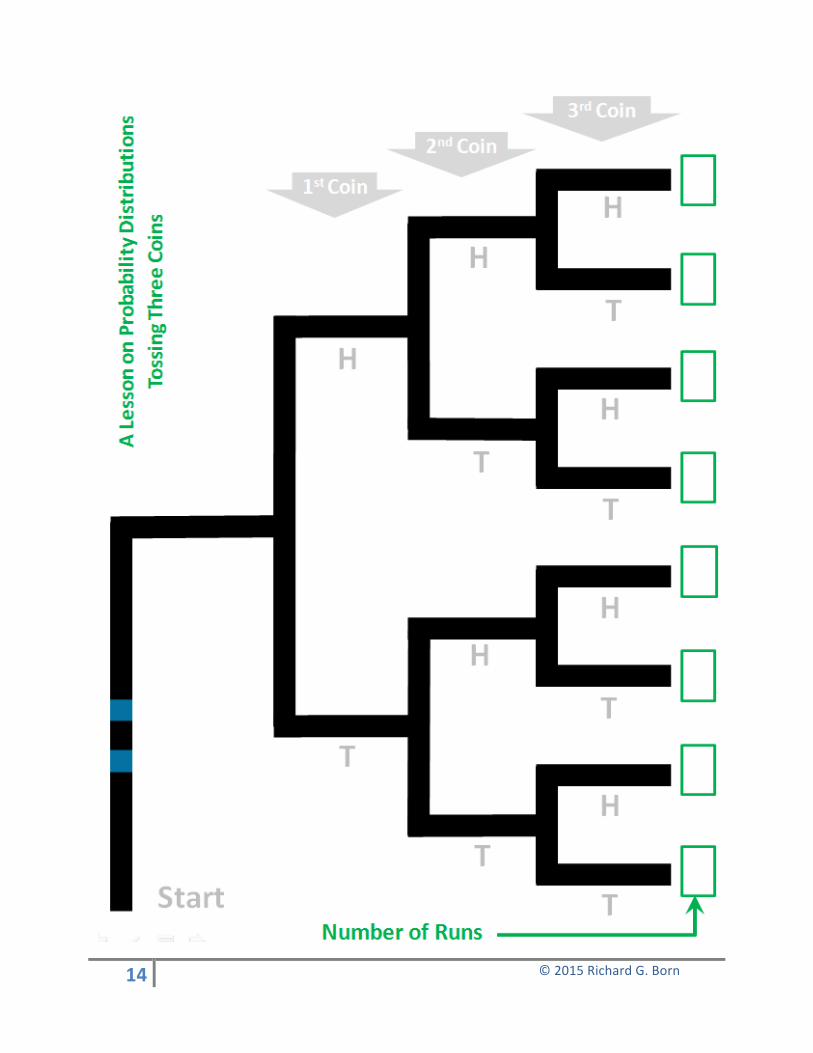
You can ask the students to make a rough sketch of an OzoMap that could be used to allow Ozobot to simulate tossing three coins. An OzoMap that does the job well is available for duplication for students on page 10. A “fast” speed code appears shortly after the start to speed up data collection during the experiment. At the first intersection Ozobot chooses one of the two possible routes each with a probability of ½. This represents the random result of tossing the first coin, either heads (H) or tails (T). Regardless of the path randomly selected by Ozobot, Ozobot then encounters another intersection with two possible choices representing the 2nd coin, each with a probability of ½. Finally, Ozobot reaches yet a third intersection with two possible choices representing the 3rd coin, each with a probability of ½. Keeping in mind the fact that Ozobot makes independent decisions at each intersection and the probability rule, the probability of the eight equally likely outcomes at the far right of the OzoMap is ½ x ½ x ½ = 1/8 = 0.125.
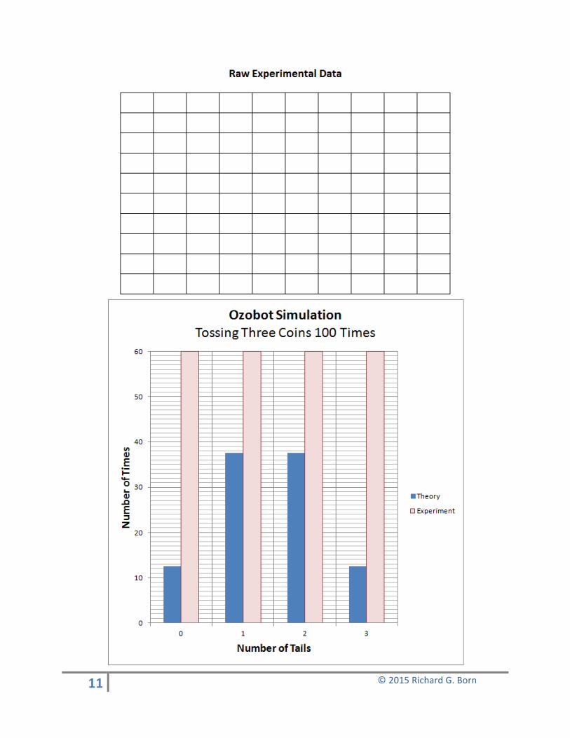
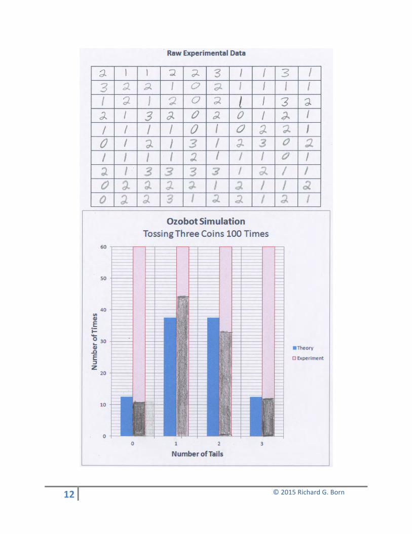
The value of the random variable number of tails is shown in green for each of the eight equally likely outcomes. Therefore, each time that Ozobot simulates tossing the three coins, the student can quickly note the number of tails encountered. The number of tails is then recorded in the Raw Experimental Data table on page 11 for 100 Ozobot simulations of the tossing of three coins. The graph shows two columns:
• The blue column contains the theoretical number of times that the number of tails is expected. This was found by multiplying the probabilities on page 8 by 100 (since there are 100 simulated tosses).
• The red column can be shaded in for the number of times each of the number of tails occurs.
Due to the randomness of the results, and the relatively small size (100) of the sample, there will be noticeable differences between student group results. An example of typical results for this experiment is shown on page 12. In this example, 0 tails were tossed 11 times, 1 tail was tossed 44 times, 2 tails were tossed 33 times, and 3 tails were tossed 12 times.

10 © 2015 Richard G. Born
11 © 2015 Richard G. Born
12 © 2015 Richard G. Born
13 © 2015 Richard G. Born
Student Exercise #1:
By now the students should have a pretty good understanding of the concepts random variable and probability distribution, as well as how to display a probability distribution either in tabular or graphical form.
Have them once again consider the Ozobot simulation for tossing three coins. But this time let’s change the random variable that we are investigating. Let’s define the random variable as the number of runs in each toss of the three coins. To explain the concept of a run, consider tossing HTT as an example. Any unbroken sequence of l ike letters is called a run, even in the sequence has only one letter. In the sequence HTT, there are 2 runs: the first run is H and the second run is TT.
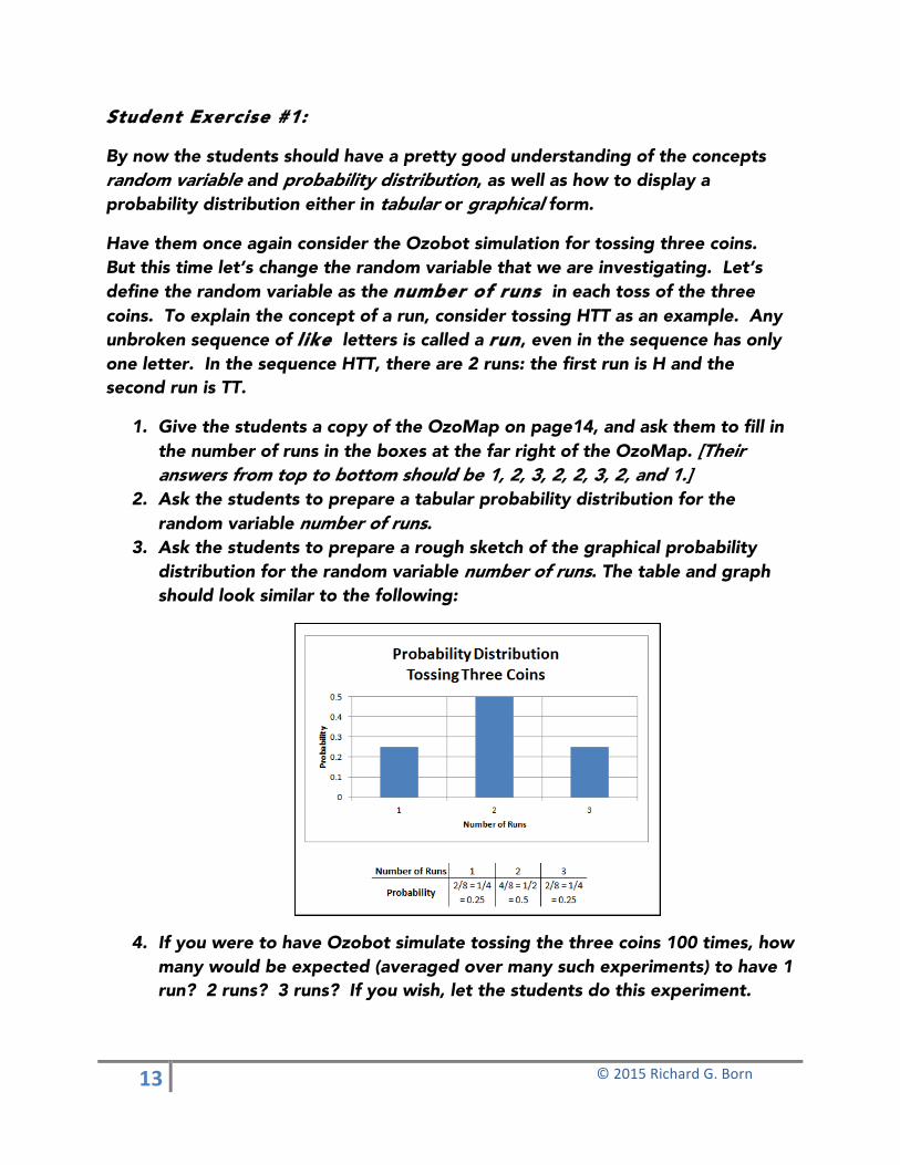
1. Give the students a copy of the OzoMap on page14, and ask them to fill in the number of runs in the boxes at the far right of the OzoMap. [Their answers from top to bottom should be 1, 2, 3, 2, 2, 3, 2, and 1.]
2. Ask the students to prepare a tabular probability distribution for the random variable number of runs.
3. Ask the students to prepare a rough sketch of the graphical probability distribution for the random variable number of runs. The table and graph should look similar to the following:
4. If you were to have Ozobot simulate tossing the three coins 100 times, how many would be expected (averaged over many such experiments) to have 1 run? 2 runs? 3 runs? If you wish, let the students do this experiment.
14 © 2015 Richard G. Born
15 © 2015 Richard G. Born
Student Exercise #2:
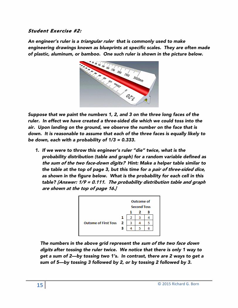
An engineer’s ruler is a triangular ruler that is commonly used to make engineering drawings known as blueprints at specific scales. They are often made of plastic, aluminum, or bamboo. One such ruler is shown in the picture below.
Suppose that we paint the numbers 1, 2, and 3 on the three long faces of the ruler. In effect we have created a three-sided die which we could toss into the air. Upon landing on the ground, we observe the number on the face that is down. It is reasonable to assume that each of the three faces is equally likely to be down, each with a probability of 1/3 ≈ 0.333.
1. If we were to throw this engineer’s ruler “die” twice, what is the probability distribution (table and graph) for a random variable defined as the sum of the two face-down digits? Hint: Make a helper table similar to the table at the top of page 3, but this time for a pair of three-sided dice, as shown in the figure below. What is the probability for each cell in this table? [Answer: 1/9 ≈ 0.111. The probability distribution table and graph are shown at the top of page 16.]
The numbers in the above grid represent the sum of the two face down digits after tossing the ruler twice. We notice that there is only 1 way to get a sum of 2—by tossing two 1’s. In contrast, there are 2 ways to get a sum of 5—by tossing 3 followed by 2, or by tossing 2 followed by 3.

16 © 2015 Richard G. Born
2. Tossing an engineer’s ruler into the air could be a bit unwieldy and also dangerous to those nearby! No problem—we can construct an OzoMap that will allow Ozobot to simulate the tossing an engineer’s ruler. Ask the students to draw a rough sketch of an OzoMap that could be used to toss an engineer’s ruler twice, with the sides painted with the numbers 1, 2, and 3. An OzoMap for such a simulation appears on page 17. Each of the three paths encountered at the first intersection that Ozobot encounters has a probability of 1/3 of being followed. Similarly, each of the three paths for the second intersection has a probability of 1/3 of being followed. By the probability rule, each of the nine outcomes has a probability of 1/3 x 1/3 = 1/9. If you wish, the OzoMap can be copied and distributed to student lab groups for doing an actual experiment. The students should be asked to fill in the boxes on the far right of the OzoMap with the values for the random variable sum of face-down digits. [Their answers from top to bottom should be 2, 3, 4, 3, 4, 5, 4, 5, and 6.] If you decide to have some of the lab groups do the experiment, you can copy the data table and chart on page 18 for students to record their data and summarize results.

17 © 2015 Richard G. Born
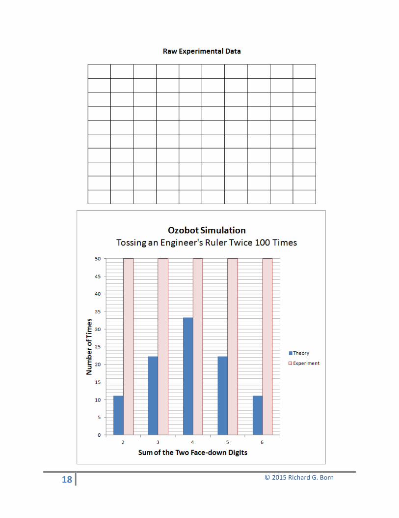
18 © 2015 Richard G. Born
19 © 2015 Richard G. Born
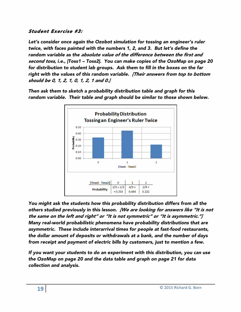
Student Exercise #3:
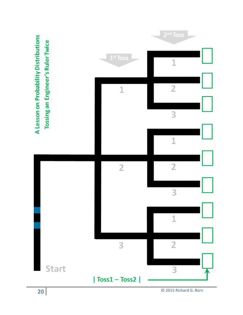
Let’s consider once again the Ozobot simulation for tossing an engineer’s ruler twice, with faces painted with the numbers 1, 2, and 3. But let’s define the random variable as the absolute value of the difference between the first and second toss, i.e., |Toss1 – Toss2|. You can make copies of the OzoMap on page 20 for distribution to student lab groups. Ask them to fill in the boxes on the far right with the values of this random variable. [Their answers from top to bottom should be 0, 1, 2, 1, 0, 1, 2, 1 and 0.]
Then ask them to sketch a probability distribution table and graph for this random variable. Their table and graph should be similar to those shown below.
You might ask the students how this probability distribution differs from all the others studied previously in this lesson. [We are looking for answers like “It is not the same on the left and right” or “It is not symmetric” or “It is asymmetric.”] Many real-world probabilistic phenomena have probability distributions that are asymmetric. These include interarrival times for people at fast-food restaurants, the dollar amount of deposits or withdrawals at a bank, and the number of days from receipt and payment of electric bills by customers, just to mention a few.
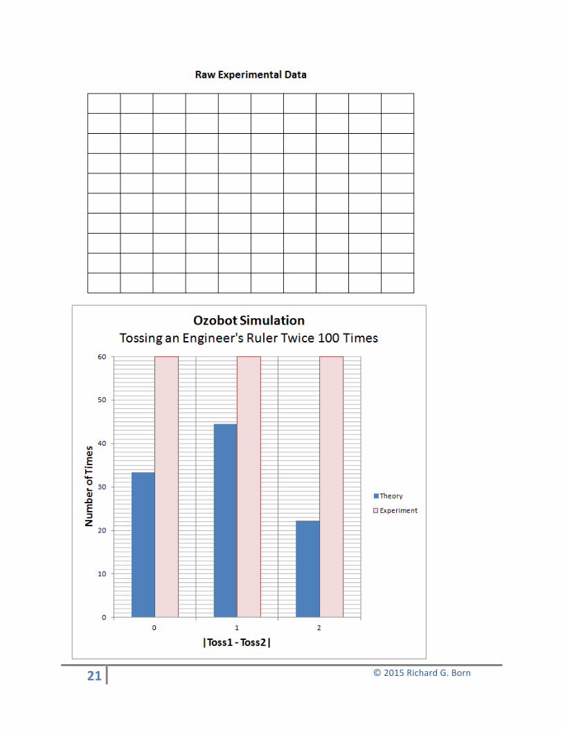
If you want your students to do an experiment with this distribution, you can use the OzoMap on page 20 and the data table and graph on page 21 for data collection and analysis.
20 © 2015 Richard G. Born
21 © 2015 Richard G. Born
22 © 2015 Richard G. Born
Suggestions for Classroom Use
A fairly large number of classroom investigations were described in this write-up. It is unlikely that you have the classroom time to have every student group perform all of the investigations. Some alternatives include:
• Discuss and have the student lab groups do the investigation in which Ozobot simulates tossing a pair of ordinary six-sided dice (pages 1 through 7).
• Time permitting, discuss and have the student lab groups do the investigation where Ozobot simulates tossing three coins (pages 8 through 14).
• Discuss and assign different lab groups different Ozobot simulations: o Tossing a Pair of Ordinary Dice with sum of faces up as the random
variable (pages 1 through 7) o Tossing Three Coins with number of tails as the random variable
(pages 8 through 12) o Tossing Three Coins with the number of runs as the random variable
(pages 13 and 14) o Tossing an Engineer’s Ruler Twice with sum of the face-down digits
as the random variable (pages 15 through 18) o Tossing an Engineer’s Ruler Twice with the absolute value of the
difference between toss1 and toss2 as the random variable (pages 19 through 21)
• Some students may have their own Ozobots at home. You could assign some of the investigations as homework.
STEM Topics
• Interdisciplinary—robotics, probability and statistics working together • Computer Science—colored visual codes are used to program a line-
following robot.
Materials
Ozobots (1 per every 3 to 4 students, fully charged)
8½” x 11” printouts of OzoMaps and Data Collection sheets for the investigations you plan to have student lab groups perform
Estimated time-frame (variable from 50 to 90 minutes)


![[DL輪読会]Deep Learning for Sampling from Arbitrary Probability Distributions](https://static.fdocument.pub/doc/165x107/5aaa85d17f8b9af9198b467f/dldeep-learning-for-sampling-from-arbitrary-probability-distributions.jpg)