Continuous Probability Distributions

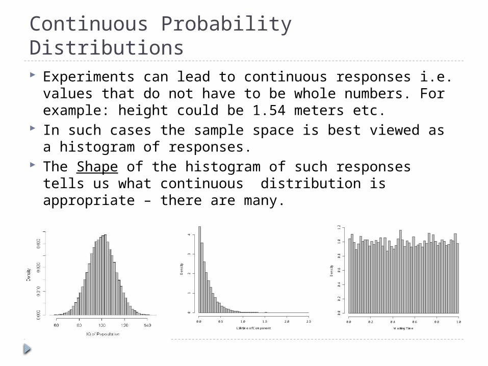
Continuous Probability Distributions Experiments can lead to continuous responses i.e.

values that do not have to be whole numbers. For example: height could be 1.54 meters etc.

In such cases the sample space is best viewed as a histogram of responses.

The Shape of the histogram of such responses tells us what continuous distribution is appropriate – there are many.

Lifetime of Component

De

nsity

0.0 0.5 1.0 1.5 2.0 2.5

01

23

4

Waiting TimeD

en

sity

0.0 0.2 0.4 0.6 0.8 1.0

0.0

0.2

0.4

0.6

0.8

1.0

1.2

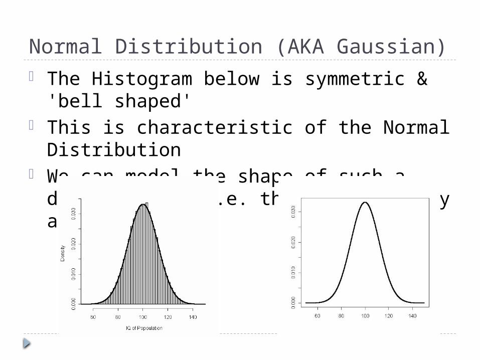
Normal Distribution (AKA Gaussian)• The Histogram below is symmetric & 'bell

shaped'• This is characteristic of the Normal

Distribution• We can model the shape of such a

distribution (i.e. the histogram) by a Curve

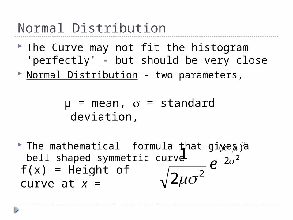
Normal Distribution The Curve may not fit the histogram

'perfectly' - but should be very close Normal Distribution - two parameters,

µ = mean, = standard deviation,

The mathematical formula that gives a bell shaped symmetric curve

f(x) = Height of curve at x =

2

2

2

)(

22

1

x

e

Normal Distribution Why Not P(x) as before?

=> because response is continuous

What is the probability that a person sampled at random is 6 foot?

Equivalent question: what proportion of people are 6 foot?

=> really mean what proportion are 'around 6 foot' ( as good as the measurement device

allows) - so not really one value, but many values close together.

Example: What proportion of graduates earn €35,000?

Would we exclude €35,000.01 or €34,999.99?

Round to the nearest €, €10, €100, €1000?

Continuous measure => more useful to get proportion from €35,000 - €40,000

Some Mathematical Jargon:

The formula for the normal distribution is formally called the normal probability density function (pdf)

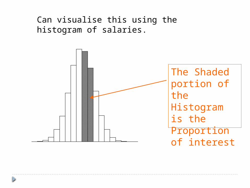
The Shaded portion of the Histogram is the Proportion of interest

Can visualise this using the histogram of salaries.

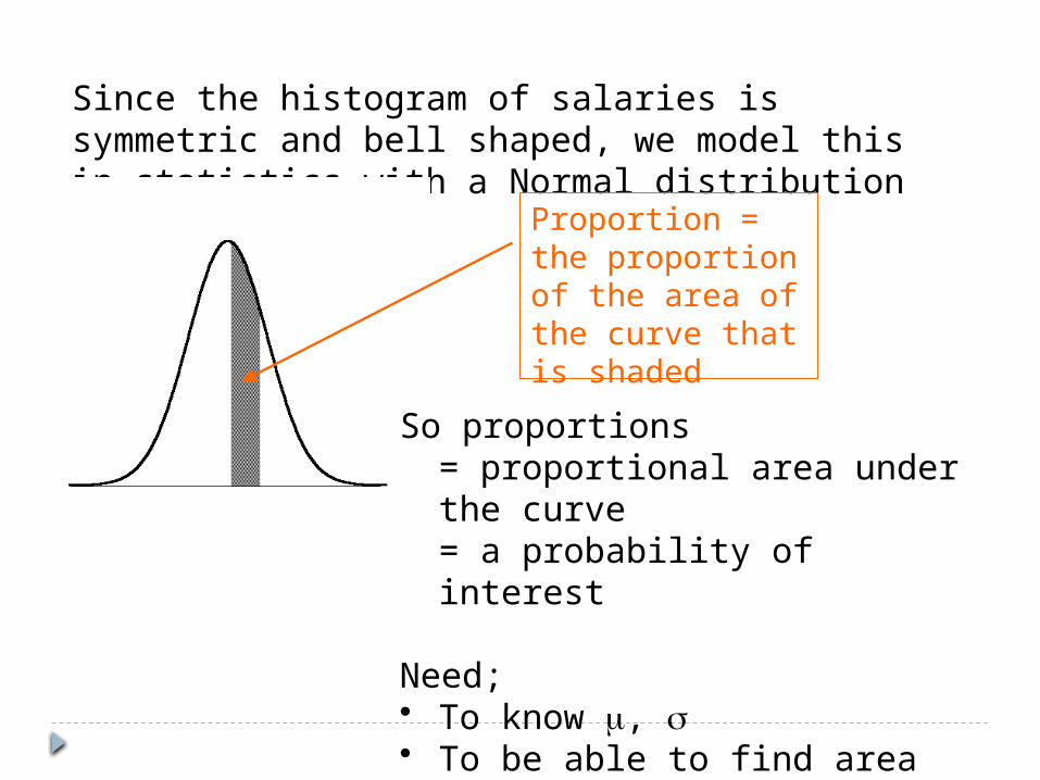
Since the histogram of salaries is symmetric and bell shaped, we model this in statistics with a Normal distribution curve.

Proportion = the proportion of the area of the curve that is shaded

So proportions = proportional area under the curve = a probability of interest

Need;• To know , • To be able to find area under

curve

Area under a curve is found using integration in mathematics.

In this case would need a technique called numerical integration.

Total area under curve is 1. However, the values we need are in

Normal Probability Tables.

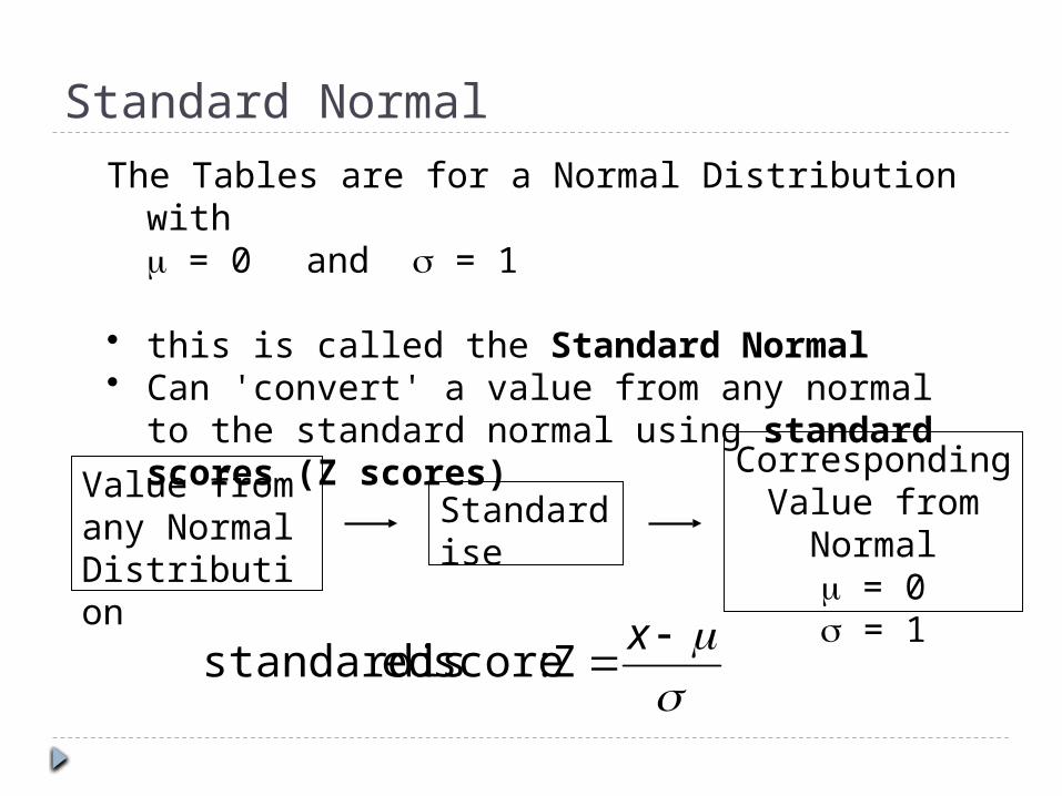
The Tables are for a Normal Distribution with = 0 and = 1

• this is called the Standard Normal• Can 'convert' a value from any normal to the

standard normal using standard scores (Z scores)

Value from any NormalDistribution

Standardise

Corresponding Value from

Normal = 0 = 1

Z :score edstandardis

x

Standard Normal

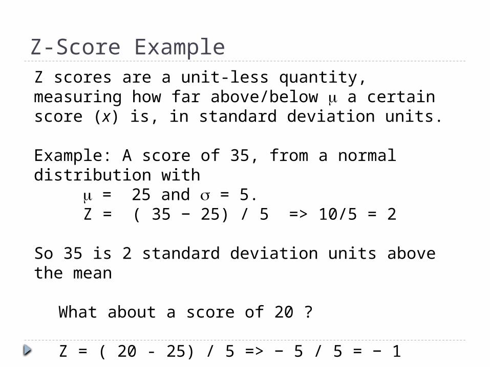
Z scores are a unit-less quantity, measuring how far above/below a certain score (x) is, in standard deviation units.

Example: A score of 35, from a normal distribution with

= 25 and = 5.Z = ( 35 − 25) / 5 => 10/5 = 2

So 35 is 2 standard deviation units above the mean

What about a score of 20 ?

Z = ( 20 - 25) / 5 => − 5 / 5 = − 1

So 20 is 1 standard unit below the mean

Z-Score Example

Positive Z score => score is above the meanNegative Z score => score is below the mean

By subtracting and dividing by the we convert any normal to = 0, =1, so only need one set of tables!

Z-Score Example

From looking at the histogram of peoples weekly receipts, a supermarket knows that the amount people spend on shopping per week is normally distributed with:

= €58 = €15.

Example:

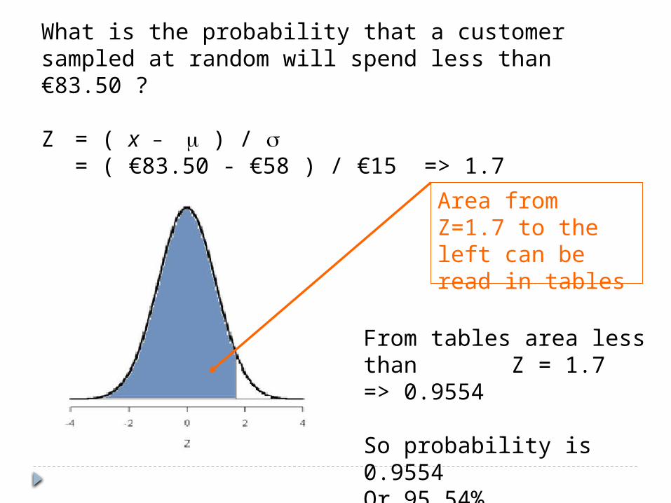
What is the probability that a customer sampled at random will spend less than €83.50 ?

Z = ( x − ) / = ( €83.50 - €58 ) / €15 => 1.7

Area from Z=1.7 to the left can be read in tables

From tables area less than Z = 1.7 => 0.9554

So probability is 0.9554 Or 95.54%

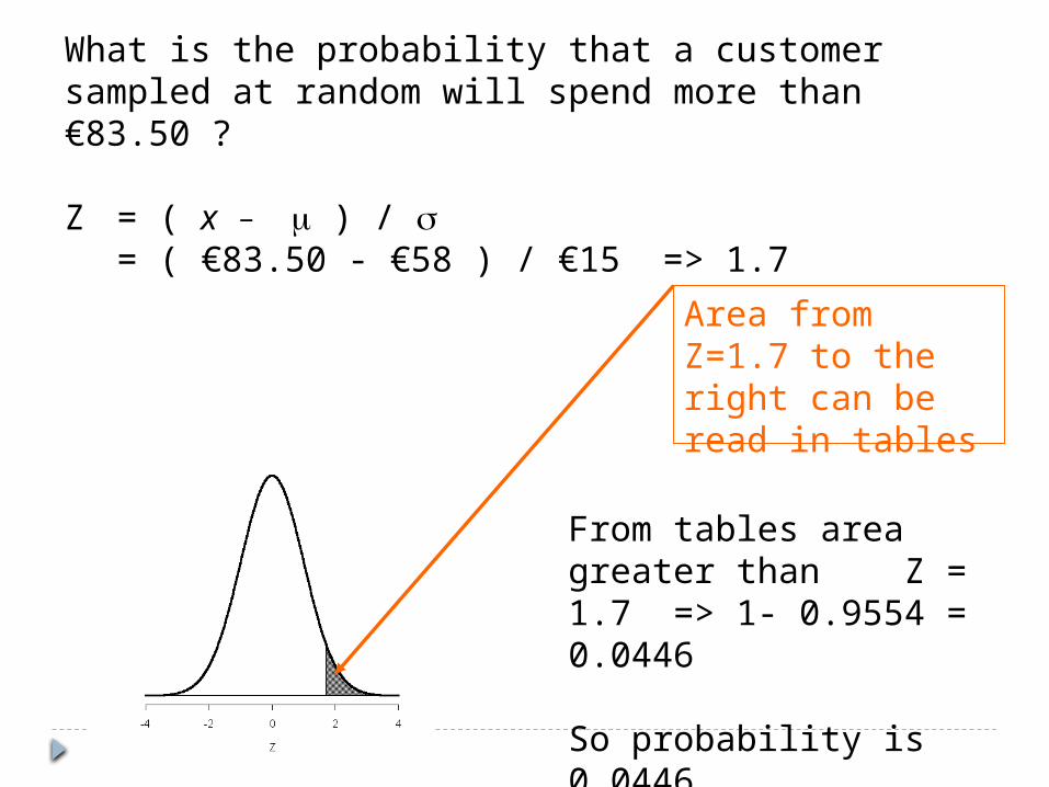
What is the probability that a customer sampled at random will spend more than €83.50 ?

Z = ( x − ) / = ( €83.50 - €58 ) / €15 => 1.7

Area from Z=1.7 to the right can be read in tables

From tables area greater than Z = 1.7 => 1- 0.9554 = 0.0446

So probability is 0.0446 Or 4.46%

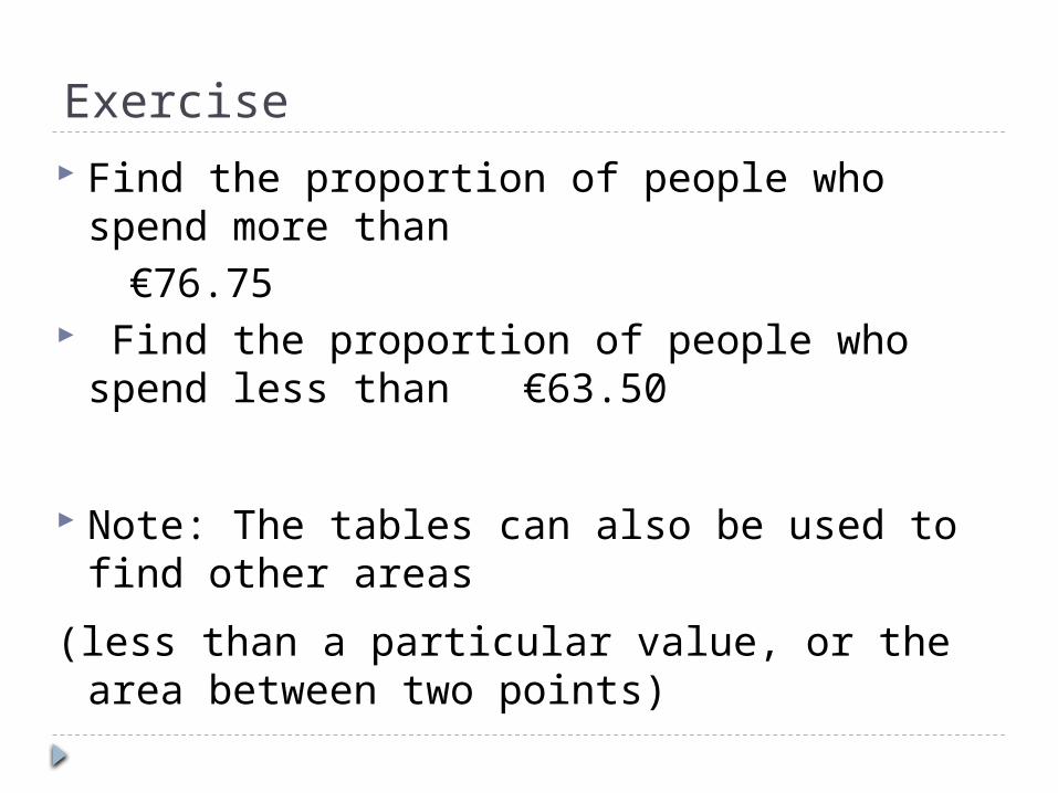
Exercise Find the proportion of people who spend

more than €76.75 Find the proportion of people who spend

less than €63.50

Note: The tables can also be used to find other areas

(less than a particular value, or the area between two points)

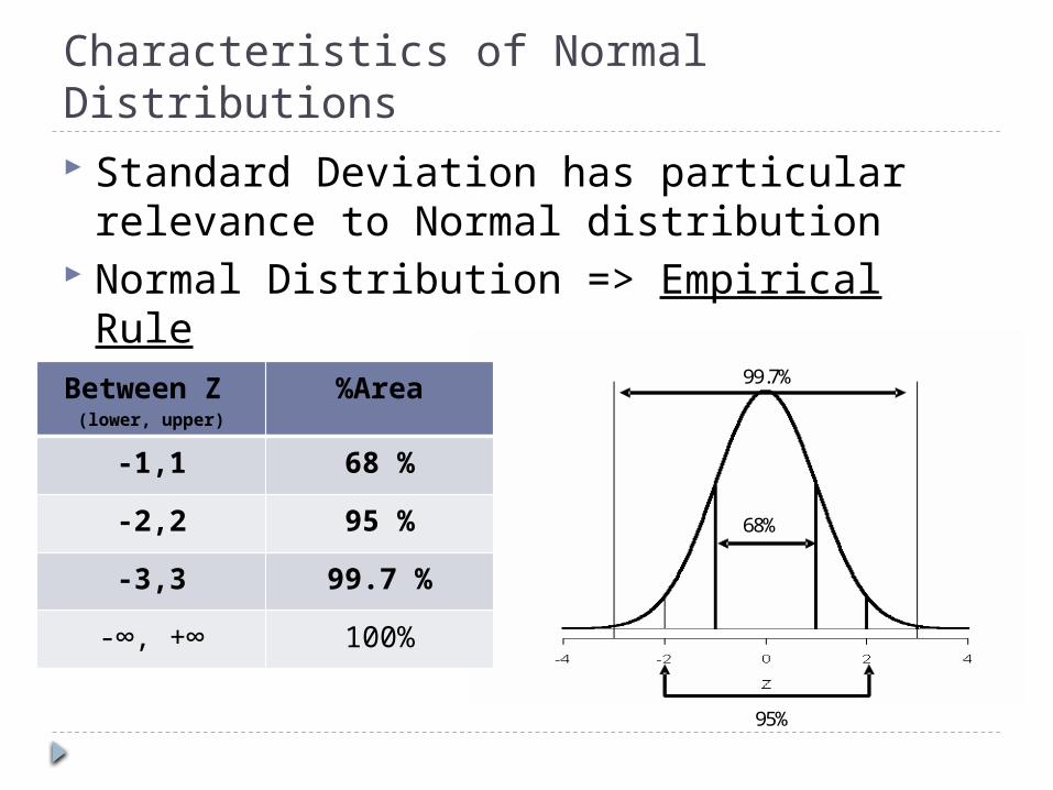
Characteristics of Normal Distributions Standard Deviation has particular

relevance to Normal distribution Normal Distribution => Empirical Rule

68%

95%

99.7% Between Z (lower, upper)

%Area

-1,1 68 %

-2,2 95 %

-3,3 99.7 %

-∞, +∞ 100%

The normal distribution is just one of the known continuous probability distributions.

Each have their own probability density function, giving different shaped curves.

In each case, we find probabilities by calculating areas under these curves using integration.

However, the Normal is the most important – as it plays a major role in Sampling Theory.

Other important continuous probability distributions include• Exponential distribution – especially positively

skewed lifetime data.

• Uniform distribution.

• Weibull – especially for ‘time to event’ analysis.

• Gamma distribution – waiting times between Poisson events in time etc.

• Many others…..

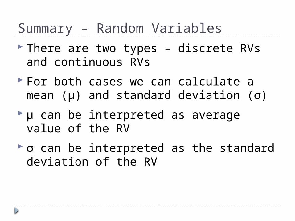
Summary – Random Variables There are two types – discrete RVs and

continuous RVs

For both cases we can calculate a mean (μ) and standard deviation (σ)

μ can be interpreted as average value of the RV

σ can be interpreted as the standard deviation of the RV

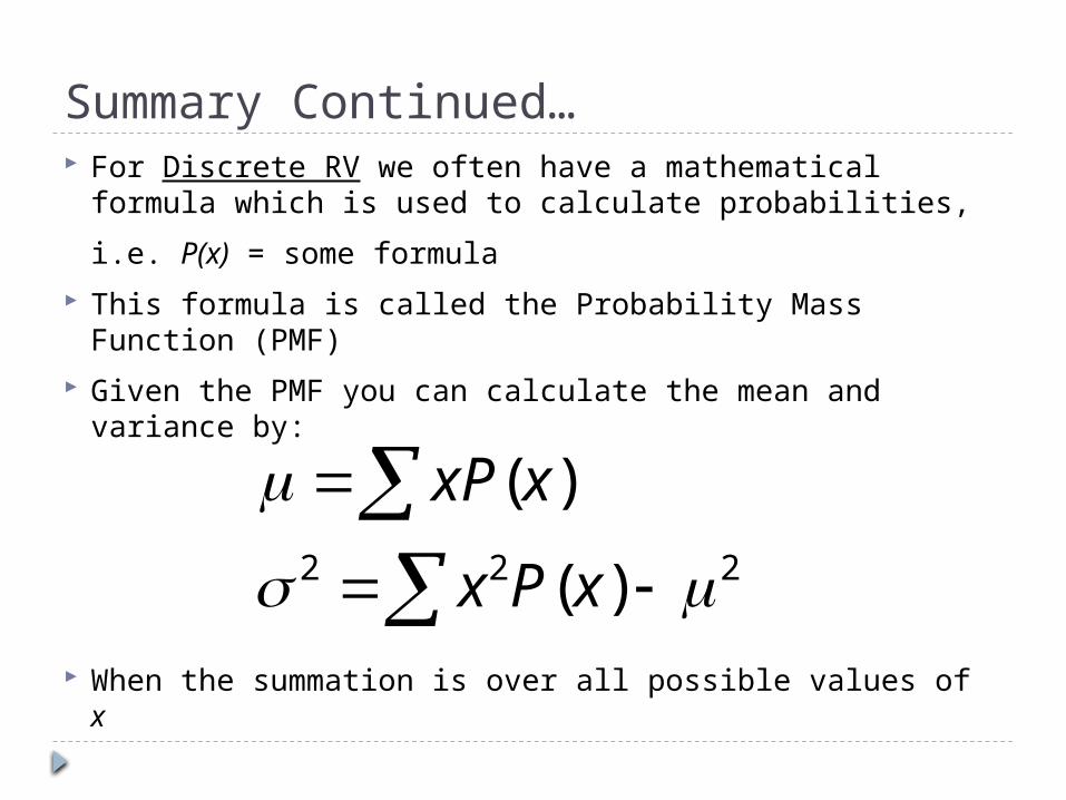
Summary Continued… For Discrete RV we often have a mathematical formula

which is used to calculate probabilities,

i.e. P(x) = some formula

This formula is called the Probability Mass Function (PMF)

Given the PMF you can calculate the mean and variance by:

When the summation is over all possible values of x

222 )(

)(

xPx

xxP

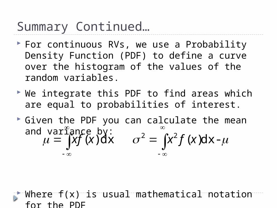
Summary Continued… For continuous RVs, we use a Probability Density

Function (PDF) to define a curve over the histogram of the values of the random variables.

We integrate this PDF to find areas which are equal to probabilities of interest.

Given the PDF you can calculate the mean and variance by:

Where f(x) is usual mathematical notation for the PDF

-dx )(dx )( 22 xfxxxf