A comparison of measurement techniques to determine the ...
4
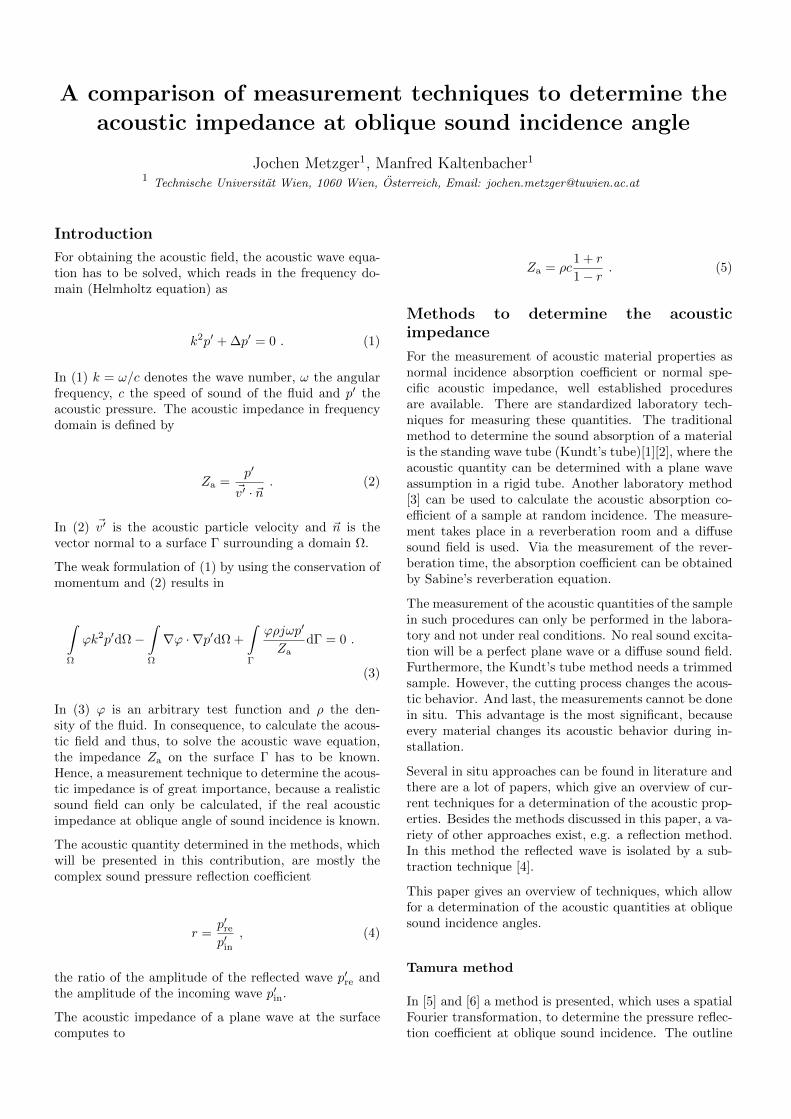
A comparison of measurement techniques to determine the acoustic impedance at oblique sound incidence angle Jochen Metzger 1 , Manfred Kaltenbacher 1 1 Technische Universit¨ at Wien, 1060 Wien, ¨ Osterreich, Email: [email protected] Introduction For obtaining the acoustic field, the acoustic wave equa- tion has to be solved, which reads in the frequency do- main (Helmholtz equation) as k 2 p 0 +Δp 0 =0 . (1) In (1) k = ω/c denotes the wave number, ω the angular frequency, c the speed of sound of the fluid and p 0 the acoustic pressure. The acoustic impedance in frequency domain is defined by Z a = p 0 ~ v 0 · ~n . (2) In (2) ~ v 0 is the acoustic particle velocity and ~n is the vector normal to a surface Γ surrounding a domain Ω. The weak formulation of (1) by using the conservation of momentum and (2) results in Z Ω ϕk 2 p 0 dΩ - Z Ω ∇ϕ ·∇p 0 dΩ + Z Γ ϕρjωp 0 Z a dΓ = 0 . (3) In (3) ϕ is an arbitrary test function and ρ the den- sity of the fluid. In consequence, to calculate the acous- tic field and thus, to solve the acoustic wave equation, the impedance Z a on the surface Γ has to be known. Hence, a measurement technique to determine the acous- tic impedance is of great importance, because a realistic sound field can only be calculated, if the real acoustic impedance at oblique angle of sound incidence is known. The acoustic quantity determined in the methods, which will be presented in this contribution, are mostly the complex sound pressure reflection coefficient r = p 0 re p 0 in , (4) the ratio of the amplitude of the reflected wave p 0 re and the amplitude of the incoming wave p 0 in . The acoustic impedance of a plane wave at the surface computes to Z a = ρc 1+ r 1 - r . (5) Methods to determine the acoustic impedance For the measurement of acoustic material properties as normal incidence absorption coefficient or normal spe- cific acoustic impedance, well established procedures are available. There are standardized laboratory tech- niques for measuring these quantities. The traditional method to determine the sound absorption of a material is the standing wave tube (Kundt’s tube)[1][2], where the acoustic quantity can be determined with a plane wave assumption in a rigid tube. Another laboratory method [3] can be used to calculate the acoustic absorption co- efficient of a sample at random incidence. The measure- ment takes place in a reverberation room and a diffuse sound field is used. Via the measurement of the rever- beration time, the absorption coefficient can be obtained by Sabine’s reverberation equation. The measurement of the acoustic quantities of the sample in such procedures can only be performed in the labora- tory and not under real conditions. No real sound excita- tion will be a perfect plane wave or a diffuse sound field. Furthermore, the Kundt’s tube method needs a trimmed sample. However, the cutting process changes the acous- tic behavior. And last, the measurements cannot be done in situ. This advantage is the most significant, because every material changes its acoustic behavior during in- stallation. Several in situ approaches can be found in literature and there are a lot of papers, which give an overview of cur- rent techniques for a determination of the acoustic prop- erties. Besides the methods discussed in this paper, a va- riety of other approaches exist, e.g. a reflection method. In this method the reflected wave is isolated by a sub- traction technique [4]. This paper gives an overview of techniques, which allow for a determination of the acoustic quantities at oblique sound incidence angles. Tamura method In [5] and [6] a method is presented, which uses a spatial Fourier transformation, to determine the pressure reflec- tion coefficient at oblique sound incidence. The outline
Transcript of A comparison of measurement techniques to determine the ...
A comparison of measurement techniques to determine the
acoustic impedance at oblique sound incidence angle
Jochen Metzger1, Manfred Kaltenbacher11 Technische Universitat Wien, 1060 Wien, Osterreich, Email: [email protected]
Introduction
For obtaining the acoustic field, the acoustic wave equa-tion has to be solved, which reads in the frequency do-main (Helmholtz equation) as
k2p′ + ∆p′ = 0 . (1)
In (1) k = ω/c denotes the wave number, ω the angularfrequency, c the speed of sound of the fluid and p′ theacoustic pressure. The acoustic impedance in frequencydomain is defined by
Za =p′
~v′ · ~n. (2)
In (2) ~v′ is the acoustic particle velocity and ~n is thevector normal to a surface Γ surrounding a domain Ω.
The weak formulation of (1) by using the conservation ofmomentum and (2) results in
∫Ω
ϕk2p′dΩ−∫Ω
∇ϕ · ∇p′dΩ +
∫Γ
ϕρjωp′
ZadΓ = 0 .
(3)
In (3) ϕ is an arbitrary test function and ρ the den-sity of the fluid. In consequence, to calculate the acous-tic field and thus, to solve the acoustic wave equation,the impedance Za on the surface Γ has to be known.Hence, a measurement technique to determine the acous-tic impedance is of great importance, because a realisticsound field can only be calculated, if the real acousticimpedance at oblique angle of sound incidence is known.
The acoustic quantity determined in the methods, whichwill be presented in this contribution, are mostly thecomplex sound pressure reflection coefficient
r =p′rep′in
, (4)
the ratio of the amplitude of the reflected wave p′re andthe amplitude of the incoming wave p′in.
The acoustic impedance of a plane wave at the surfacecomputes to
Za = ρc1 + r
1− r. (5)
Methods to determine the acousticimpedance
For the measurement of acoustic material properties asnormal incidence absorption coefficient or normal spe-cific acoustic impedance, well established proceduresare available. There are standardized laboratory tech-niques for measuring these quantities. The traditionalmethod to determine the sound absorption of a materialis the standing wave tube (Kundt’s tube)[1][2], where theacoustic quantity can be determined with a plane waveassumption in a rigid tube. Another laboratory method[3] can be used to calculate the acoustic absorption co-efficient of a sample at random incidence. The measure-ment takes place in a reverberation room and a diffusesound field is used. Via the measurement of the rever-beration time, the absorption coefficient can be obtainedby Sabine’s reverberation equation.
The measurement of the acoustic quantities of the samplein such procedures can only be performed in the labora-tory and not under real conditions. No real sound excita-tion will be a perfect plane wave or a diffuse sound field.Furthermore, the Kundt’s tube method needs a trimmedsample. However, the cutting process changes the acous-tic behavior. And last, the measurements cannot be donein situ. This advantage is the most significant, becauseevery material changes its acoustic behavior during in-stallation.
Several in situ approaches can be found in literature andthere are a lot of papers, which give an overview of cur-rent techniques for a determination of the acoustic prop-erties. Besides the methods discussed in this paper, a va-riety of other approaches exist, e.g. a reflection method.In this method the reflected wave is isolated by a sub-traction technique [4].
This paper gives an overview of techniques, which allowfor a determination of the acoustic quantities at obliquesound incidence angles.
Tamura method
In [5] and [6] a method is presented, which uses a spatialFourier transformation, to determine the pressure reflec-tion coefficient at oblique sound incidence. The outline

y
x
0
sample
z
loudspeakerz0
z1
z2
Figure 1: Outline of the measurement principle in theTamura method. The Loudspeaker placed at z0 and the twomeasurement planes at z1 and z2 are shown.
of the measurement principle can be seen in Fig. 1. Asound source, radiating spherical waves into a three di-mensional space, is placed at z0 above a sample. Thesurface of the sample coincides with the xy plane. Inthis method the pressure distribution on two planes (z1,z2) has to be measured. This can either be realized byone microphone on a scanner or with a microphone ar-ray [7]. In [6] a number of 200 measurement points isreported.
By two-dimensional Fourier transform
P (kx, ky, z) =
∫ ∫p′e−j(kxx+kyy)dxdy , (6)
the complex pressure distribution is decomposed intoplane-wave components. In case of a pressure amplitudeof a wave, which travels from the plane z2 to z1, thepressure at z1 can be calculated by [5]
P (kx, ky, z1) = P (kx, ky, z2)ejkz(z1−z2) , (7)
where kz =√k2 − k2
x − k2y is the wave number in z-
direction. The pressure reflection coefficient can be com-puted by separating the incident and reflected plane wavecomponent
r =P (kx, ky, z2)e−jkzz1 − P (kx, ky, z1)e−jkzz2
P (kx, ky, z1)ejkzz2 − P (kx, ky, z2)ejkzz1(8)
at the angle of sound incidence
Θ = sin−1[√
k2x + k2
y/k0
]. (9)
This measurement method is a very time-consuming (incase of a scanner with one microphone) or a costly (incase of a microphone array) technique. Moreover, therewill be errors in calculating the pressure reflection coef-ficient, because the spatial resolution in measuring thepressure distribution is not infinite and the measurementplanes cannot be infinitely wide.
Two microphone method
In [8] a measurement technique is presented, which deter-mines the normal acoustic impedance at oblique anglesof sound incidence with two microphones in a free fieldwith no reflections. An outline of the measurement setupis shown in Fig. 2. Two microphones M1 and M2 withthe distances d1 and d2 are placed above a sample. Thesample is located on a rigid surface and the sound inci-dence at angle Θ is realized by means of a loudspeakerwith distance r0 to the surface of the sample.
d
samplerigid surface
loudspeaker
r0
1
2d
M1
MM2
Θ
Figure 2: Outline of the measurement principle in the twomicrophone method. The loudspeaker is placed at angle Θat distance r0. M1 and M2 with a distances d1 and d2 areplaced above a sample.
The pressure reflection coefficient at M (surface of thesample) for a plane wave computes to
rp =
e−jkd2 cos Θ − p2
p1e−jkd1 cos Θ
p2
p1ejkd1 cos Θ − ejkd2 cos Θ
. (10)
As shown in [8], a small distance between loudspeakerand sample provides insufficient results, because the waveat the sample is not plane. Therefore, a spherical-waveapproximation is supposed in [8] and the spherical pres-sure reflection coefficient calculates as
rs =
1
r2ejkr2 − p2
p1
1
r1ejkr1
p2
p1
1
r′1ejkr
′1 − 1
r′2ejkd2
. (11)
In (11) r1 and r2 are the distances between loudspeakerand M1 and M2 and r′1 and r′2 are the distances betweenthe mirror source (reflected loudspeaker at the rigid sur-face) and M1 and M2. The acoustic impedance at asound incidence of angle Θ computes to
Za,s =1
cos Θ
rs + 1
rs − 1
jkr0
jkr0 − 1. (12)
Measured impedance of a glass fiber at 2 kHz and 3 kHzin comparison to the impedance obtained by a modelare shown in [9]. The distance between loudspeaker andsample r0 was about 4 m, whereas d1 = 1.5 cm and d2 =0.5 cm. The surface of the panel was about 1 m2. Theresults show good agreement at those two frequencies forangles of sound incidence up to 60.
In situ method
An easy and quick method to determine the pressure re-flection coefficient is proposed in [10]. This method isbased on a simultaneous measurement of sound pressureand particle velocity in contrast to the previous describedmethods, where only the sound pressure is measured. InFig. 3 the measurement principle with a pu-probe placedat distance hs − h in front of a loudspeaker is shown. Atfirst, the method with sound incidence of angle 0 is dis-cussed and first measurement results are shown. Theimpedance at free radiation a) Zff and the impedancenear the sample b) Zmeas has to be measured. Withthe assumption, that the sound source radiates sphericalwaves, the pressure reflection coefficient can be calculatedby
r =
Zmeas
Zff− 1
Zmeas
Zff
(hs − hhs + h
)(jk(hs + h) + 1
jk(hs − h) + 1
)+ 1
hs + h
hs − hejk2h
(13)
with h, the distance between pu-probe and sample.
h - hshs
pmeas
vmeas
h - hs
pff
vffsample
a) b)
Figure 3: Outline of the measurement principle in the insitu method. a) Freefield measurement b) Measurement ofthe impedance at distance h above a sample.
The pu-probe we used, is the Microflown Ultimate SoundProbe (USP), capable of measuring the acoustic pressureand the particle velocity in 3D. We calibrated the USPby means of our simultaneous calibration technique [11]and identified the orientation of the USP by using theACCMF-system [12]. The ACCMF-system is a combi-nation of a 3D acceleration sensor and the USP in orderto know the direction of the particle velocity sensor bymeans of the local gravity field.
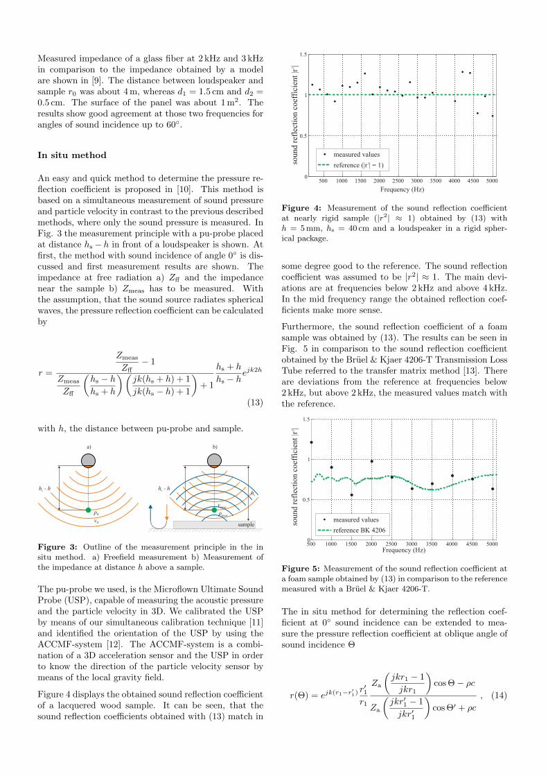
Figure 4 displays the obtained sound reflection coefficientof a lacquered wood sample. It can be seen, that thesound reflection coefficients obtained with (13) match in
500 1000 1500 2000 2500 3000 3500 4000 4500 50000
0.5
1
1.5
Frequency (Hz)
soun
d re
flec
tion
coe
ffic
ient
|r |
measured values
reference (|r | = 1)
2
2
Figure 4: Measurement of the sound reflection coefficientat nearly rigid sample (|r2| ≈ 1) obtained by (13) withh = 5 mm, hs = 40 cm and a loudspeaker in a rigid spher-ical package.
some degree good to the reference. The sound reflectioncoefficient was assumed to be |r2| ≈ 1. The main devi-ations are at frequencies below 2 kHz and above 4 kHz.In the mid frequency range the obtained reflection coef-ficients make more sense.
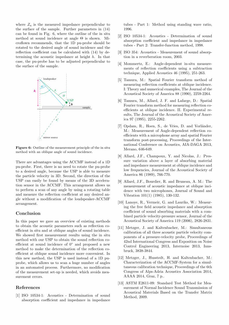
Furthermore, the sound reflection coefficient of a foamsample was obtained by (13). The results can be seen inFig. 5 in comparison to the sound reflection coefficientobtained by the Bruel & Kjaer 4206-T Transmission LossTube referred to the transfer matrix method [13]. Thereare deviations from the reference at frequencies below2 kHz, but above 2 kHz, the measured values match withthe reference.
soun
d re
flec
tion
co
effi
cien
t |r
|2
500 1000 1500 2000 2500 3000 3500 4000 4500 50000
0.5
1
1.5
Frequency (Hz)
measured values
reference BK 4206
Figure 5: Measurement of the sound reflection coefficient ata foam sample obtained by (13) in comparison to the referencemeasured with a Bruel & Kjaer 4206-T.
The in situ method for determining the reflection coef-ficient at 0 sound incidence can be extended to mea-sure the pressure reflection coefficient at oblique angle ofsound incidence Θ
r(Θ) = ejk(r1−r′1) r′1
r1
Za
(jkr1 − 1
jkr1
)cos Θ− ρc
Za
(jkr′1 − 1
jkr′1
)cos Θ′ + ρc
, (14)
where Za is the measured impedance perpendicular tothe surface of the sample. Further parameters in (14)can be found in Fig. 6, where the outline of the in situmethod at sound incidence at angle Θ is shown. Mi-croflown recommends, that the 1D pu-probe should berotated to the desired angle of sound incidence and thereflection coefficient can be calculated with (14) by de-termining the acoustic impedance at height h. In thatcase, the pu-probe has to be adjusted perpendicular tothe surface of the sample.
r`
r1hs
h
1
sample
loudspeaker
mirror source
USP
Θ
Θ`
Figure 6: Outline of the measurement principle of the in situmethod with an oblique angle of sound incidence.
There are advantages using the ACCMF instead of a 1Dpu-probe. First, there is no need to rotate the pu-probeto a desired angle, because the USP is able to measurethe particle velocity in 3D. Second, the direction of theUSP can easily be found by means of the 3D accelera-tion sensor in the ACCMF. This arrangement allows usto perform a scan of any angle by using a rotating tableand measure the reflection coefficient at any desired an-gle without a modification of the loudspeaker-ACCMFarrangement.
Conclusion
In this paper we gave an overview of existing methodsto obtain the acoustic parameters such as reflection co-efficient in situ and at oblique angles of sound incidence.We showed first measurement results using the in situmethod with our USP to obtain the sound reflection co-efficient at sound incidence of 0 and proposed a newmethod to make the determination of the reflection co-efficient at oblique sound incidence more convenient. Inthis new method, the USP is used instead of a 1D pu-probe, which allows us to scan a huge number of anglesin an automated process. Furthermore, no modificationof the measurement set-up is needed, which avoids mea-surement errors.
References
[1] ISO 10534-1: Acoustics - Determination of soundabsorption coefficient and impedance in impedance
tubes - Part 1: Method using standing wave ratio,1996.
[2] ISO 10534-1: Acoustics - Determination of soundabsorption coefficient and impedance in impedancetubes - Part 2: Transfer-function method, 1998.
[3] ISO 354: Acoustics - Measurement of sound absorp-tion in a reverberation room, 2003.
[4] Mommertz, E.: Angle-dependent in-situ measure-ments of reflection coefficients using a subtractiontechnique, Applied Acoustics 46 (1995), 251-263.
[5] Tamura, M.: Spatial Fourier transform method ofmeasuring reflection coefficients at oblique incidence.I: Theory and numerical examples, The Journal of theAcoustical Society of America 88 (1990), 2259-2264.
[6] Tamura, M., Allard, J. F. and Lafarge, D.: SpatialFourier transform method for measuring reflection co-efficients at oblique incidence. II. Experimental re-sults, The Journal of the Acoustical Society of Amer-ica 97 (1995), 2255-2262.
[7] Opdam, R., Hoen, S., de Vries, D. and Vorlander,M.: Measurement of Angle-dependent reflection co-efficients with a microphone array and spatial Fouriertransform post-processing, Proceedings of the Inter-national Conference on Acoustics, AIA-DAGA 2013,Merano, 646-649.
[8] Allard, J.F., Champoux, Y. and Nicolas, J.: Pres-sure variation above a layer of absorbing materialand impedance measurement at oblique incidence andlow frequencies, Journal of the Acoustical Society ofAmerica 86 (1989), 766-770.
[9] Allard, J.F., Bourdier, R. and Bruneau, A. M.: Themeasurement of acoustic impedance at oblique inci-dence with two microphones, Journal of Sound andVibration 101(1) (1985), 130-132.
[10] Lanoye, R., Vermeir, G. and Lauriks, W.: Measur-ing the free field acoustic impedance and absorptioncoefficient of sound absorbing materials with a com-bined particle velocity-pressure sensor, Journal of theAcoustical Society of America 119 (2006), 2826-2831.
[11] Metzger, J. and Kaltenbacher, M.: Simultaneouscalibration of all three acoustic particle velocity com-ponents of a pressure-velocity probe, Proceedings of42nd International Congress and Exposition on NoiseControl Engineering 2013, Internoise 2013, Inns-bruck, 3838-3844.
[12] Metzger, J., Husstedt, H. and Kaltenbacher, M.:Characterization of the ACCMF-System for a simul-taneous calibration technique, Proceedings of the 6thCongress of Alps-Adria Acoustics Association 2014,AAAA 2014, Graz, 7 p..
[13] ASTM E2611-09: Standard Test Method for Mea-surement of Normal Incidence Sound Transmission ofAcoustical Materials Based on the Transfer MatrixMethod, 2009.