A Brief Introduction to Brownian

Motion on a Riemannian Manifold

Elton P. Hsu

Department of Mathematics, Northwestern University

nkita

テキストボックス

Contents

Introductory Remarks 1

Lecture 1. Brownian Motion on a Riemannian Manifold 31.1. Brownian motion on euclidean space 31.2. Laplace-Beltrami operator and the heat kernel 41.3. Brownian motion on a Riemannian manifold 61.4. Brownian motion by embedding 81.5. Brownian motion in local coordinates 9

Lecture 2. Brownian Motion and Geometry 112.1. Radially symmetric manifolds 112.2. Radial process 132.3. Comparison theorems 15

Lecture 3. Stochastic Calculus on manifolds 173.1. Orthonormal frame bundle 173.2. Eells-Elworhthy-Malliavin construction of Brownian motion 183.3. Stochastic horizontal lift 193.4. Stochastic integrals on a manifold 21

Lecture 4. Analysis on Path and Loop Spaces 234.1. Quasi-invariance of the Wiener measure 234.2. Gradient operator 274.3. Integration by parts 284.4. Ornstein Uhlenbeck operator 304.5. Logarithmic Sobolev inequality 314.6. Concluding remarks 33

Bibliography 35

3

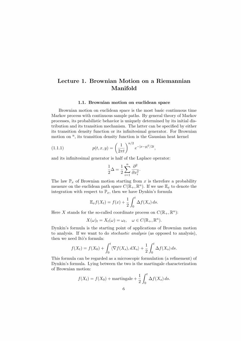
Introductory Remarks

These lecture notes constitute a brief introduction to stochastic analysison manifolds in general, and Brownian motion on Riemannian manifolds inparticular. Instead of going into detailed proofs and not accomplish much,I will outline main ideas and refer the interested reader to the literaturefor more thorough discussion. This is especially true for the last lecture, inwhich I only discuss the flat space case. Therefore it should be only servedas a guide to what one should expect for the path and loop spaces over aRiemannian manifold.

I thank Professor I. Shigekawa and other Japanese probabilists for invit-ing me to participate the Summer School in Kyushu.

1

nkita

テキストボックス

　

Lecture 1. Brownian Motion on a RiemannianManifold

1.1. Brownian motion on euclidean space

Brownian motion on euclidean space is the most basic continuous timeMarkov process with continuous sample paths. By general theory of Markovprocesses, its probabilistic behavior is uniquely determined by its initial dis-tribution and its transition mechanism. The latter can be specified by eitherits transition density function or its infinitesimal generator. For Brownianmotion on n, its transition density function is the Gaussian heat kernel

(1.1.1) p(t, x, y) =(

12πt

)n/2

e−|x−y|2/2t,

and its infinitesimal generator is half of the Laplace operator:

12∆ =

12

n∑i=1

∂2

∂x2i

.

The law Px of Brownian motion starting from x is therefore a probabilitymeasure on the euclidean path space C(R+, Rn). If we use Ex to denote theintegration with respect to Px, then we have Dynkin’s formula

Exf(Xt) = f(x) +12

∫ t

0∆f(Xs) ds.

Here X stands for the so-called coordinate process on C(R+, Rn):

X(ω)t = Xt(ω) = ωt, ω ∈ C(R+, Rn).

Dynkin’s formula is the starting point of applications of Brownian motionto analysis. If we want to do stochastic analysis (as opposed to analysis),then we need Ito’s formula:

f(Xt) = f(X0) +∫ t

0〈∇f(Xs), dXs〉+

12

∫ t

0∆f(Xs) ds.

This formula can be regarded as a microscopic formulation (a refinement) ofDynkin’s formula. Lying between the two is the martingale characterizationof Brownian motion:

f(Xt) = f(X0) + martingale +12

∫ t

0∆f(Xs) ds.

3

4 LECTURE 1. BROWNIAN MOTION ON A RIEMANNIAN MANIFOLD

All these formulations (Dynkin’s formula, Ito’s formula, martingale charac-terization) are equivalent in the sense that each one of them defines uniquelythe probability measure Px under which the coordinate process is a Markovprocess with the Gaussian transition density function (1.1.1).

All of the above formulations of Brownian motion will find its counter-part when Rn is replaced by a Riemannian manifold.

As a way of thinking, it is useful to regard paths of Brownian motionas the characteristic lines of the Laplace operator ∆. Since ∆ is an ellipticoperator, we know that it has no real characteristic lines in the classicalsense. It is a basic fact in the theory of partial differential equations thatthe solution of the initial value problem is a weighted average of the data onthe characteristic lines emanating from the point at which we are seekingsolution. Take, for example, the initial value problem for the wave equation

∂2u

∂t2=

∂2u

∂x2, u(0, x) = f(x),

∂u

∂x(0, x) = 0.

The characteristic lines of the wave operator are x± t = const. The solutionof the problem is

u(t, x) =f(x + t) + f(x− t)

2,

which is the expected value of the initial value f(x + t) and f(x − t) onthe characteristic lines from (x, t) as if we assign each characteristic line theprobability 1/2. Now consider the Dirichlet problem on the smooth domainD in Rn:

∆u = 0 on D,

u = f on ∂D.

Each curve X starting from x meets the boundary at XτD , where τD is thefirst exit time of D:

τD = inf t ≥ 0 : Xt 6∈ D .

The value of the data for this “characteristic line” is f(XτD). The prob-ability is assigned to these “characteristic lines” according to the law ofBrownian motion Px. In analogy with the case of the wave equation, wearrive heuristically the formula

uf (x) = Exf(XτD), x ∈ D,

which is Doob’s representation of the solution of the Dirichlet problem.

1.2. Laplace-Beltrami operator and the heat kernel

As we have seen in Section 1.1, the Laplace operator and the Gauss-ian transition density function (heat kernel) are the basic analytic objectsassociated with Brownian motion on Rn. Of the two, the Laplace operatoris the more fundamental one and the heat kernel can be obtained as (mini-mal) fundamental solution of the heat equation associated with the Laplace

1.2. LAPLACE-BELTRAMI OPERATOR AND THE HEAT KERNEL 5

operator, namely, the function p(t, x, y) is the smallest positive solution ofthe following initial value problem:

∂p

∂t=

12∆u, lim

t↓0p(t, x, y) = δx(y).

The counterpart of the Laplace operator on a Riemannian manifold Mis the Laplace-Beltrami operator ∆M , which will serves as the infinitesimalgenerator for Brown motion on M . This operator can be briefly describedas follows. We denote the Riemannian metric on M 〈·, ·〉x. The gradientgradf of a function f on M is a vector field on M defined uniquely by

〈grandf,X〉 = X(f), X ∈ Γ (M).

[Here Γ (M) is the space of smooth vector field on M .] The divergence divXof a vector field X is characterized by∫

MX(f)dµ = −

∫M

fdivX dµ.

Here µ is the Riemannian volume measure. The Laplace-Beltrami operatoris

∆Mf = div(gradf).In local coordinates x1, · · · , xn, the Riemannian metric is written in the form

ds2 = gijdxidxj .

The Laplace-Beltrami operator is given by

∆Mf =1√G

∂

∂xj

(√Ggij ∂f

∂xi

).

Here G is the determinant of the matrix gij andgij

is its inverse. We

have

∆Mf = gij ∂2f

∂xi∂xj+ bi ∂f

∂xi,

where

bi =1√G

∂(√

Ggij)∂xj

= gjkΓ ijk,

where Γ ijk are the Christoffel symbols of the metric ds2 in the local coor-dinates. Therefore ∆M is a second order, strictly elliptic operator.

The construction of the heat kernel (minimal fundamental solution)p(t, x, y) associated with the Laplace-Beltrami operator is not a trivial taskand belongs to the fields of partial differential equations and differential ge-ometry. It is carried out in great detail in Chavel[1]. We will see later thatthe theory of stochastic differential equations allows in some sense avoid thisconstruction.

A general stochastic differential equation in Stratonovich formulationhas the form

dXt = Vα(X)t dWαt + V0(Xt) dt.

6 LECTURE 1. BROWNIAN MOTION ON A RIEMANNIAN MANIFOLD

It generates a diffusion process (i.e., Markov process with continuous samplepaths) whose infinitesimal generator is

L =12

l∑i=1

V 2α + V0.

Thus it has the form of a “sum of squares.” Unfortunately, on a general Rie-mannian manifold, there is no natural way of writing the Laplace-Beltramioperator as a sum of squares. Such a representation of ∆M is possible if Mis embedded isometrically in some euclidean space ∆l. For a point x ∈ M ,let Pα denote the projection of the unit coordinate vector ξα on the tangentspace TxM . We obtain in this way l vector fields Pα on M . It can be shownthat ([11], 77–78)

∆M =l∑

α=1

P 2α.

According to Nash’s theorem, one can always embedd a Riemannian man-ifold isometrically in some euclidean space. This fact and the above ex-pression for ∆M can be used to give an extrinsic construction of Brownianmotion on M .

1.3. Brownian motion on a Riemannian manifold

We define Brownian motion on M to be a Markov process whose transi-tion density function is p(t, x, y), the heat kernel associated with the Laplace-Beltrami operator. General theory of Markov processes shows how such aprocess can be constructed, see Chung[4]. It turns out to be a diffusionprocess, i.e., a strong Markov process with continuous sample paths.

On a general Riemannian manifold it may happen that∫M

p(t, x, y)dy < 1.

Probabilistically this means that Brownian motion may not run for all time.More precisely, there is a finite stopping time e, called the lifetime of Brow-nian motion such that

limt↑↑e

Xt =∞M .

where M = M∪∞M is the one-point compactification of M and the abovelimit is understood in the topology of M . Intuitively speaking, Brownianmotion may go off the manifold in a finite amount of time. Naturally thiscase does not happen if M is compact. We have

Px e ≥ t =∫

Mp(t, x, y) dy.

When Px e <∞ = 1 for some x and t (hence for all x and t), we say thatthe manifold M is stochastically complete. We will address the questionwhen a Riemannian manifold is stochastically complete.

1.3. BROWNIAN MOTION ON A RIEMANNIAN MANIFOLD 7

Once Brownian motion is constructed as a diffusion processes with tran-sition density function p(t, x, y), the fact that p(t, x, y) is the minimal fun-damental solution of the heat equation for the Laplace-Beltrami operatorgive immediately Dynkin’s formula

Exf(Xt) = f(x) + Ex

∫ t

0∆Mf(Xs) ds

for all reasonable functions on M , say smooth with compact support. With-out little extra effort, this can be expended to read

(1.3.1) f(Xt) = f(X0) + Mft +

12

∫ t

0∆f(Xs) ds, 0 ≤ t < e.

Here Mf is a (local) martingale depending on f . The quadratic variationprocess of Mf can be identified.

Proposition 1.3.1. We have

〈Mf 〉t =∫ t

0|∇f(Xs)|2ds.

Proof. We decompose f(Xt)2 in two ways. First, we use Ito’s formulaand (1.3.1) to obtain

f(Xt)2 = f(x)2 + 2∫ t

0f(Xs) df(Xs) + 〈Mf 〉t

= f(x)2 + 2∫ t

0f(Xs)dMf

s +∫ t

0f(Xs)∆Mf(Xs) ds + 〈Mf 〉t.

Second we use (1.3.1) with f replaced by f2 and obtain

f(Xt)2 = f(x)2 + Mf2

t +12

∫ t

0∆M (f2)(Xs) ds.

Equating the bounded variation parts of the two expressions, we have

〈Mf 〉t =12

∫ t

0

∆M (f2)(Xs)− 2f(Xs)∆Mf(Xs)

ds.

Finally,∆M (f2)− 2f∆Mf = 2|∇f |2.

We thus have established the following fact about Brownian motion onM :

f(Xt) = f(X0) + Mft +

12

∫ t

0∆Mf(Xs) ds, 0 ≤ t < e,

with where Mf is a local martingale with

〈Mf 〉t =∫ t

0|∇f(Xs)|2ds.

8 LECTURE 1. BROWNIAN MOTION ON A RIEMANNIAN MANIFOLD

This is property of Brownian motion is sufficient for most applications inanalysis and geometry, for in these applications we rarely need to knowthe joint distribution of the martingale Mf and the stochastic integral∫ t

0∆Mf(Xs) ds. For more delicate stochastic analysis, we need to have

an explicit description of the martingale Mf . If M = Rn, we have

Mft =

∫ t

0〈∇f(Xs), dXt〉.

In the present formulation of Brownian motion, there is not a direct way ofwriting down Mf .

1.4. Brownian motion by embedding

If M is a submanifold of a euclidean space Rl, Brownian motion onM can be obtained by solving a stochastic differential equation on M . InSection 1.2 we mentioned that the Laplace-Beltrami operator ∆M can bewritten in the form of a sum of squares:

∆M =l∑

α=1

P 2α,

where Pα is the projection of the αth coordinate unit vector ξα on thetangent space TxM . Each Pα is a vector field on M . Consider the followingStratonovich stochastic differential equation on M driven by a l-dimensionaleuclidean Brownian motion W :

(1.4.1) dXt = Pα(Xt) dWαt , X0 ∈M.

[The summation convention is used.] This is a stochastic differential equa-tion on M because Pα are vector fields on M . Extending Pα arbitrarily tothe whole ambient space we can solve this equation as if it is an equation onRl by the usual Picard’s iteration. It can be verified that if the initial valueX0 lies on the manifold M , then the solution lies on M for all time:

Px Xt ∈M for all t < e|X0 ∈M = 1,

see [11], 22–23. Furthermore, the solution is a diffusion process generatedby (1/2)

∑lα=1 P 2

α = (1/2)∆M . Using Ito’s formula we have

f(Xt) = f(X0) + Mft +

12

∫ t

0∆Mf(Xs) ds, 0 ≤ t < e,

where

Mft =

∫ t

0〈Pαf(Xs), dWα

s 〉.

Example 1.4.1. (Brownian motion on a sphere) Consider the unit sphereSn canonically embedded in Rn+1. The projection to the tangent sphere atx is given by

P (x) ξ = ξ − 〈ξ, x〉x, x ∈ Sn, ξ ∈ Rn+1.

1.5. BROWNIAN MOTION IN LOCAL COORDINATES 9

Hence the matrix P = P1, · · · , Pn+1 is

P (x)ij = δij − xixj .

Brownian motion on Sn is the solution of the stochastic differential equation

Xit = Xi

0 +∫ t

0(δij −Xi

sXjs ) dW j

s , X0 ∈ Sn.

This is Stroock’s representation of spherical Brownian motion.

The representation 1.4.1 is a good way to visualize Brownian motionon M as a pathwise object (rather than a measure on the path spaceC(R+,M)). It is an extrinsic representation because it depends on theembedding of M into some euclidean space Rl. It has the drawback thatthe equation (1.4.1) is driven by a Brownian motion W whose dimensionl is in general larger than the dimension n of the manifold M , whereas insome sense Brownian motion on M should still be an n-dimensional object.Full strength of Brownian motion on M can only be revealed after we writeit faithfully as an n-dimensional object, i.e., as the solution of a stochasticdifferential equation driven by an n-dimensional euclidean Brownian motion.

1.5. Brownian motion in local coordinates

As we have mentioned in Section 1.2, the Laplace-Beltrami operatorcan be written as

∆Mf =1√G

∂

∂xj

(√Ggij ∂f

∂xi

).

This gives a way of constructing Brownian motion valid up to the first timeit exits from the local coordinate chart. Let σ =

σj

i

be the unique sym-

metric square root of g−1 =gij

. Consider the solution of the stochastic

differential equation for a process Xt =X1

t , . . . , Xnt

:

dX it = σi

j(Xt) dBjt +

12bi(Xt) dt.

Then it is easy to verify by Ito’s formula that X is a diffusion processgenerated by (1/2)∆M , i.e., X is a Brownian motion on M . Brownianmotion can be studied this way by choosing an appropriate local coordinatesystem in which the Laplace-Beltrami operator ∆M takes special a specialform.

Lecture 2. Brownian Motion and Geometry

We study the effect of curvature on the behavior of Brownian motionand hope that it will lead to interesting results about the manifold itself. Wewill concentrate some problems which can be studied through the distancefunction r(x) = d(x, o), where o is a fixed point on the manifold. In thisrespect, the radial process rt = r(Xt) is a natural object of investigation.We often compare this process with the same process on a radially symmet-ric manifold satisfying certain curvature conditions. On such a manifold,problems often becomes one-dimensional and can be solved explicitly.

2.1. Radially symmetric manifolds

A radially symmetric manifold M has a distinguished point o, call thepole of M . In the polar coordinates (r, θ) induced by the exponential mapexpo : Rn →M based at o, the metric has the following form

ds2 = dr2 + G(r)2dθ2.

Here dθ2 denotes the standard Riemannian metric on the n−1-sphere Sn−1,and G is a smooth function on an interval [0, D) satisfying

G(0) = 0, G′(0) = 1, 0 ≤ r < D.

In terms of these coordinates, the Laplace-Beltrami operator has the formThe Laplace-Beltrami operator has the form

(2.1.1) ∆M = Lr +1

G(r)2∆Sn−1 ,

where Lr is the radial Laplacian

Lr =(

∂

∂r

)2

+ (n− 1)G′(r)G(r)

∂

∂r,

and ∆Sn−1 is the Laplace-Beltrami operator on Sn−1. The main featureof this case is that the radial component is completely decoupled from theangular component and the angular component is a scaling of ∆msn−1 withthe scale 1/G(r)2 depending on the radial component. In the terminologyof differential geometry, the metric ds2 has the form of a warped product.

Let Xt = (rt, θt) be a Brownian motion on a radially symmetric manifoldM written in polar coordinates. Using polar coordinates, we find that the

11

12 LECTURE 2. BROWNIAN MOTION AND GEOMETRY

radial component is the solution of the stochastic differential equation:

(2.1.2) rt = r0 + Wt +n− 1

2

∫ t

0

G′(rs)G(rs)

ds,

where W is a 1-dimensional Brownian motion. The angular component canalso be described easily. Let Y = Yt be a Brownian motion on Sn−1

independent of W (hence also independent of rt). Define a new time scale

(2.1.3) lt =∫ t

0

ds

G(rs)2,

and let θt = Ylt be the time change of the spherical Brownian motion Y .Then Xt = (rt, θt) constructed this way is a Brownian motion on M (see[11], 84–85). From this description of Brownian motion it is clear that thebehavior of Brownian motion on a radially symmetric manifold is controlledby and large by its radial process. The radially process is a one-dimensionaldiffusion process, which has been well studied in probability theory.

Let’s study a special case more closely. A complete, simply connectedmanifolds of negative sectional curvature is called a Cartan-Hadamard man-ifold. Suppose that M is such a manifold with constant negative curvature−K2 (space form). Then it is a radially symmetric manifold with the metricds2 = dr2 + G(r)2dθ2 is given by

G(r) =sinhKr

K.

The behavior of Brownian motion on this manifold is typical for Brownianmotion on Cartan-Hadamard manfiold whose curvature is pinned betweentwo negative constant.

The radial process is the solution of

drt = dWt +n− 1

2K coth Krt dt.

We write the equation in the form

rt = Wt +(n− 1)

2

∫ t

0K coth Krs ds.

We have cothKrt ≥ 1 for all t because rt ≥ 0. Hence

(2.1.4) rt ≥ r0 + Wt +(n− 1)

2K t.

According to the law of the iterated logarithm,

lim supt→∞

Wt√2t ln ln t

= 1,

Thus the term r0 + Wt on the right side of (2.1.4) is of lower order than thelast term and we have (with probability one) rt →∞. Now that cothKrt →1 as t→∞, from

rt

t=

r0 + Wt

t+

(n− 1)2

K

t

∫ t

0coth Krs ds

2.2. RADIAL PROCESS 13

we find the asymptotic behavior of the radial process

(2.1.5) limt→∞

rt

t=

(n− 1)K2

.

We now examine at the angular process. From the above discussion, weknow that it is a time-change of a Brownian motion on the sphere Sn−1. Inthe present case, the time change is

lt =∫ t

0

(K

sinhKrs

)2

ds.

From (2.1.5) the integral converges as t ↑ ∞. It follows that

(2.1.6) limt→∞

θt = Yl∞ .

(2.1.5) and (2.1.6) give a fairly good picture of the asymptotic behaviorof Brownian motion on a complete, simply connected manifold of constantnegative curvature.

See [12] for more recent work on angular convergence of Brownian mo-tion and its relation with the Dirichlet problem at infinity for Cartan-Hadamard manifolds.

2.2. Radial process

The concept of a radial process can be introduced for Brownian motionon a general Riemannian manifold M . Fix a reference point o ∈ M , andlet r(x) = d(x, o) be the Riemannian distance between x and o. We definethe radial process rt = r(Xt). It is natural to try to use Ito’s formula todecompose this into a martingale part and a bounded variation part. Thefunction r : M → R+ has a well behaved singularity at the origin. Inparticular,

∆Mr ∼ n− 1r

near r = 0.

This singularity will not cause any problem for us because, except for thetrivial one-dimensional case, Brownian motion X never hits o for t > 0.However, x 7→ r(x) is not a smooth function on M\ o. Differential geom-etry ([8] tells us exactly where it is smooth.

For simplicity we assume that M is geodesically complete. Every ge-odesic segment can be extended in both directions indefinitely and everypair of points can be connected by a distance-minimizing geodesic. For eachunit vector e ∈ ToM , there is a unique geodesic Ce : [0,∞)→ M such thatCe(0) = e. The exponential map exp : ToM →M is

exp te = Ce(t).

If we identify ToM with Rn by an orthonormal frame, the exponential mapbecomes a map from Rn onto M . For small t, the geodesic Ce[0, t] is theunique distance-minimizing geodesic between its endpoints. Let t(e) be the

14 LECTURE 2. BROWNIAN MOTION AND GEOMETRY

largest t such that the geodesic Ce[0, t] is distance-minimizing from Ce(0) toCe(t). Define

Co = t(e)e : e ∈ ToM, |e| = 1 .

Then the cutlocus of o is the set Co = exp Co. Sometimes we also call Co

the cutlocus of o. The set within the cutlocus is the star-shaped domain

Eo = te ∈ ToM : e ∈ ToM, 0 ≤ t < t(e), |e| = 1 .

On M the set within cutlocus is Eo = exp Eo. We have the following basicresults from differential geometry (see [8] [2] [3]).

Theorem 2.2.1. (i) The map exp : Eo → Eo is a diffeomorphism.(ii) The cutlocus Co is a closet subset of measure zero.(iii) If x ∈ Cy, then y ∈ Cx.(iv) Eo and Co are disjoint and M = E0 ∪ Co.

According to the above theorem the polar coordinates (r, θ) are wellbehaved on the region M\Co within the cutlocus. The set they do not coveris the cutlocus Co, a set of measure zero. The radial function r(x) = d(x, o)is smooth on M\Co and Lipschitz on all of M . Furthermore, |∇r| = 1everywhere on M\Co.

If X is a Brownian motion on M starting within Eo, then, before it hitsthe cutlocus Co,

(2.2.1) r(Xt) = r(X0) + Wt +12

∫ t

0∆Mr(Xs) ds, t < TCo ,

where TCo is the first hitting time X of the cutlocus Co and W is a martin-gale. Its quadratic variation is

〈W 〉t =∫ t

0Γ (r, r)(Xs) ds =

∫ t

0|∇r(Xs)|2 ds = t.

Hence by Levy’s criterion, W is a Brownian motion. (2.2.1) shows thatthe behavior of the radial process is largely controlled by the Laplacian ofthe distance function ∆Mr. In practice we try to bound ∆Mr by a knownfunction of r and then control r(Xt) by comparing it with a one-dimensionaldiffusion process.

(2.2.1) is good enough if the cutlocus Co is empty, e.g., if M is a Cartan-Hadamard manifold. What happens to the when Brownian motion crossesthe cutlocus? Very complicated. A very detailed study of this problem canbe found in [6]. In most cases, the following result due to W. Kendall issufficient.

Theorem 2.2.2. Suppose that X is a Brownian motion on Riemannianmanifold M . Let r(x) = d(x, o) be the distance function from a fixed pointo ∈ M . Then there exist a one-dimensional euclidean Brownian motion

2.3. COMPARISON THEOREMS 15

W and a nondecreasing process L which increases only when Xt ∈ Co (thecutlocus of o) such that

r(Xt) = r0 + Wt +12

∫ t

0∆Mr(Xs) ds− Lt, t < e.

According this theorem, we always have a lower bound

rt ≤ r0 + Wt +12

∫ t

0∆Mr(Xs) ds, t < e.

If we need to bound the radial process from above, we have to assume thatthe cutlocus is empty. In this case,

r(Xt) = r0 + Wt +12

∫ t

0∆Mr(Xs) ds, t < e.

2.3. Comparison theorems

The next step is to study the Laplacian ∆Mr of the distance function.The goal is to bound ∆Mr by a simple function of r. There is a host ofLaplacian (more generally, Hessian) comparison theorems of this type onecan draw from differential geometry (see [3] [15]). We cite two simpleones which compare an arbitrary Riemannian manifold with manifolds ofconstant curvature (see [15]).

Theorem 2.3.1. Let KM (x) denote any sectional curvature at x ∈ Mand assume that

−K21 ≤ KM (x) ≤ K2

2 .

Then we have at any smooth point of the distance function r(x),

(n− 1)K2 cot K2r(x) ≤ ∆Mr(x) ≤ (n− 1)K1 coth K1r(x).

This result can be used to control the radial process, or more precisely,to compare the radial process on M with those on manifolds of constantcurvatures K2

1 and −K22 . Let’s first bound the radial process from below.

We have

rt ≤ r0 + Wt +12

∫ t

0∆Mr(Xs) ds.

Next, consider the equation

r1t = r0 + Wt +

n− 12

∫ t

0K1 coth K1r

1s ds.

r1t is the radial process of a Brownian motion on the space form of constant

curvature −K21 . Note that it is driven by the same Brownian motion W .

Since we have ∆Mr(x) ≤ (n−1)K1 coth K1r(x), the drift of rt is smaller thatthe drift of r1

t . By the standard comparison theorem for one-dimensionalprocesses (see [13]), we have rt ≤ r1

t for all t ≥ 0.

16 LECTURE 2. BROWNIAN MOTION AND GEOMETRY

Next, if M does not have cutlocus, or if t ≤ TCo , we have

rt = r0 + Wt +12

∫ t

0∆Mr(Xs) ds.

This time we compare with the process r2t determined by

r2t = r0 + Wt +

n− 12

∫ t

0K2 cot K2r

2s ds.

r2t is the radial process on the (n − 1)-dimensional sphere of radius 1/K2.

By the same argument as before, we have rt ≥ r2t .

Let’s see two applications. The next result is due to S. T. Yau.

Theorem 2.3.2. Let M be a complete manifold whose sectional curva-ture is bounded from below by a constant. Then it is stochastically complete,i.e., ∫

Mp(t, x, y) dy = 1

for all x ∈M, t > 0.

Proof. If M is not stochastically complete, that Brownian motionblows up with positive probability, i.e., it goes to infinity in finite amountof time. Suppose that KM (x) ≥ −K2

1 . Then we have shown that rt ≤ r2t . If

rt goes to infinity in finite amount of time, certain r2t will do the same. But

we have shown that rt ∼ (n− 1)Kt/2 as t→∞, which means that r2t does

not blow up. Nor will rt.

We say that Brownian motion on M is transient if for some x ∈ M(hence for all x ∈M),

Px

limt↑↑e

Xt =∞M

= 1.

Otherwise, we say Brownian motion is recurrent on M . There is a simpleanalytic criterion for recurrence and transience. Let

G(x, y) =∫ ∞

0p(t, x, y) dt

be Green’s function of M . Then Brownian motion on M is transient if andonly if G(x, y) < ∞ for some pair of points x 6= y (hence for all such pairsof points). It is well known that euclidean Brownian motion of dimension 1and 2 is recurrent, and of dimension 3 or higher is transient.

Theorem 2.3.3. Suppose that M is a Cartan-Hadamard manifold ofdimension greater than 2. Then Brownian motion on M is transient.

Proof. M does not have cutlocus and KM (x) ≤ 0. Therefore rt ≥ r2t ,

where r2t is the radial process of euclidean Brownian motion of dimension

n. Since r2t → ∞ as t ↑ ∞, we must have rt → ∞ as t ↑↑ e, which means

Brownian motion on M must be transient.

More refined results along these lines can be found in [11].

Lecture 3. Stochastic Calculus on manifolds

From a theoretical point of view, the most satisfactory construction ofBrownian motion on a manifold is that of Eells-Elworthy-Malliavin.

3.1. Orthonormal frame bundle

Let Ox(M) be the set of orthonormal frames of the tangent space TxM .The orthonormal frame bundle

O(M) =⋃

x∈M

Ox(M)

has a natural structure of a smooth manifold of dimension n(n + 1)/2. Letπ : O(M) → M be the canonical projection. Each element u ∈ O(M) istherefore an isometry

u : Rn → TπuM.

Let u ∈ O(M) and πu = x. The fibre π−1x = OxM is naturally a smoothsubmanifold of dimension n(n − 1)/2. Its tangent space VuO(M) is a sub-space of the same dimension of the full tangent space TuO(M). A curve utin O(M) is horizontal if ut is the parallel transport of u0 along the projectioncurve πut. The set of tangent vectors of horizontal curves passing througha fixed point u ∈ O(M) is the horizontal subspace HuO(M) of dimension nof TuO(M) and we have the relation

TuO(M) = HuO(M)⊕ VuO(M),

and the projection π : O(M)→M induces an isomorphism π∗ : HuO(M)→TxM . On the orthonormal frame bundle, we have n well defined horizontalvector field Hi. At each u ∈ O(M), Hi(u) is the unique horizontal vectorin HuO(M) whose projection is the ith unit vector uei of the orthonormalframe; i.e.,

π∗Hi(u) = uei, Hi(u) ∈ HuO(M).

The operator

∆O(M) =n∑

i=1

H2i

is called Bochner’s horizontal Laplacian on O(M). The Eells-Elworthy-Malliavin construction is based on the following relation.

17

18 LECTURE 3. STOCHASTIC CALCULUS ON MANIFOLDS

Proposition 3.1.1. For any smooth function f on M , we have

∆Mf(x) = ∆O(M)(f π)(u)

for any u ∈ O(M) such that πu = x.

3.2. Eells-Elworhthy-Malliavin construction of Brownian motion

We note that ∆O(M) is in the form of the sum of n squares, where n isthe dimension of the manifold M . Of course the price to pay is that it is anoperator on a much larger space O(M) instead of on the manifold M itself.Consider the following stochastic differential equation on O(M):

dUt =n∑

i=1

Hi(Ut) dW it .

It is driven by an n-dimensional Brownian motion W . A solution of thisequation is called a horizontal Brownian motion (on O(M)). It is a diffusionprocess generated by ∆O(M). Ito’s formula takes the following form:

F (Ut) = F (U0) +n∑

i=1

∫ t

0HiF (Us) dW i

s +12

∫ t

0∆O(M)F (Us) ds,

where F is a smooth function on O(M). Now, if we apply this to a functionof the form F = f π, the lift of a smooth function f on M , then byProposition 3.1.1,

f(Xt) = f(X0) +n∑

i=1

∫ t

0Hi(f π)(Us) dW i

s +12

∫ t

0∆Mf(Xs) ds.

Here Xt = πUt is the projection of the horizontal Brownian motion Ut onthe manifold M . It follows that Xt is a Brownian motion on M startingfrom X0 = πU0.

Suppose that we want to construct a Brownian motion starting fromx. We fix an orthonormal frame u ∈ O(M) over x, i.e., πu = x. There isa unique horizontal Brownian motion Ut starting from the frame u. Theprojection Xt = πUt is a Brownian motion from x. This Brownian motionis not uniquely determined by the driving Brownian motion W becausethe initial frame u can be chosen arbitrarily. Of course, the law of X iscompletely determined by the initial point x and does not depend on thechoice of either u or W . Once a frame u is fixed, W 7→ X establishes ameasure preserving map

J : (Po(Rn), µ)→ (Px(M), ν),

where µ is the Wiener measure on the euclidean path space Po(Rn) =Co(R+, Rn) (the law of euclidean Brownian motion) and ν is the law ofBrownian motion on M starting from x. The map J is usually called the Itomap for the reason that it is obtained through solving an Ito type stochastic

3.3. STOCHASTIC HORIZONTAL LIFT 19

differential equations. We will see later that this map is invertible. Theimage X = JW is called a stochastic development of W .

3.3. Stochastic horizontal lift

In differential geometry, a smooth curve on M can be lifted to a hori-zontal curve with the help of the Riemannian connection (or equivalently,the concept of parallel transport). If c : I → M is such a curve, we choosea frame u(0) over c(0 and simply let u(t) be the parallel transport of u(0)along c[0, t], which is accomplished by solving an ordinary differential equa-tion in local charts. The lift u(t), t ∈ I in turn defines a smooth curve win Rn by

w(t) = u(t)−1c(t).

The curve w is called an anti-development of c. The standard reference forthis part of differential geometry is [14].

A similar procedure can be carried out if the smooth curve c is replacedby a Brownian motion, or more generally, a semimartingale X on M . Weexpect that the horizontal lift U of X is obtained by solving a stochasticdifferential equation driven by X. Unlike a smooth curve on M , a semi-martingale on M is not a local object. A construction of U using local chartsis possible but technically unwieldy. If we assume that M is embedded insome euclidean space, then a relatively clean construction is possible.

Before we proceed further, let us give the definition of a semimartingaleon M . Let (Ω,F∗, P) be a probability space with filtration F∗ = Ft, t ≥ 0.A semimartingale X = Xt, t ≥ 0 on M is an M -valued, F∗-adapted pro-cess such that f(Xt), t ≥ 0 is a real-valued semimartingale for all smoothfunctions f on M .

Let M be a submanifold of Rl and recall that Pα(x) is the projectionof the αth coordinate unit vector ξα to the tangent space TxM at x ∈ M .Suppose that X is a semimartingale on M . Since M is a submanifold of Rl,X can be regarded as a semimartingale on Rl, i.e., X =

X1, . . . , X l

. Let

P ∗α(u) be the horizontal lift of Pα(πu) to u ∈ O(M). Then we obtain l hor-

izontal vector field. Consider the following stochastic differential equationon O(M) driven by X:

(3.3.1) dUt =l∑

α=1

P ∗α(Ut) dXα

t .

It has a unique solution once an initial frame U0 is given.

Theorem 3.3.1. The solution of (3.3.1) is a horizontal lift of X toO(M).

Proof. We sketch a proof, see [11] for details.

20 LECTURE 3. STOCHASTIC CALCULUS ON MANIFOLDS

The proof is based on the following identity which holds for any semi-martingale X on M :

(3.3.2) Xt = X0 +l∑

α=1

∫ t

0Pα(Xs) dXα

s .

This can be regarded as a stochastic differential equation for X on M .Laurent Schwartz observed once that every semimartingale on a manifoldM is a solution of a stochastic differential equation on M .

Let f : O(M)→M ⊆ Rl be the projection π : O(M)→M regarded asan Rl-valued function on O(M). Let Yt = f(Ut) = πUt. We have to showthat Yt = Xt. Apply Ito’s formula to f(Ut), we obtain

Yt = Y0 +l∑

α=1

P ∗αf(Us) dXα

s .

A not so difficult calculation shows that

P ∗αf(u) = Pα(πu).

Hence

Yt = Y0 +l∑

α=1

Pα(Ys) dXαs .

Therefore Y satisfies the same stochastic differential equation as X (see(3.3.2)). By the uniqueness of solutions we must have X = Y = πU ; namely,U is a horizontal lift of X.

Once we have found the horizontal lift U of X, it is not hard to writedown the anti-development of X:

Wt =∫ t

0U−1

s Pα(Us) dXαs .

It can be verified easily that this Rl-valued semimartingale drives an equa-tion for U , namely,

dUt =n∑

i=1

Hi(Ut) dW it .

Furthermore, if X is a Brownian motion on M , then W is a Brownian motionon Rn. This can be verified using Levy’s criterion.

The correspondences

W ←→ U ←→ X

are very useful because it converts a manifold-valued process X into a eu-clidean space valued process W , which is much easier to handle. We em-phasize two points: (1) these correspondences are valid for any M -valuedsemimartingale X; (2) they depend on the connection we have used to definehorizontal lift for vectors. Here we used the Riemannian connection, but thewhole construction can be carried out for any affine connection ∇. In this

3.4. STOCHASTIC INTEGRALS ON A MANIFOLD 21

case the orthonormal frame bundle O(M) should be replaced by the generallinear frame bundle F (M), otherwise everything remains the same.

3.4. Stochastic integrals on a manifold

As applications of the concepts of stochastic horizontal lift and anti-development, we define some stochastic integrals on a manifold.

Let X be a semimartingale and U and X its horizontal lift and anti-development, respectively. Let θ a 1-form on M . The stochastic line integralof θ along X[0, t] is defined by∫

X[0,t]θ =

n∑i=1

∫ t

0θ(Usei) dW i

s .

It can be verified that this definition is independent of the choice of theconnection. It is possible to write some other definitions in which the con-nection does not show up. For example, if M is a submanifold of Rl, thenwe have ∫

X[0,t]=

l∑α=1

∫ t

0θ(Pα)(X) dXα

t .

If θ = df is an exact 1-form, then∫X[0,t]

θ = f(Xt)− f(X0).

Another interesting fact is that the stochastic anti-development W itself is astochastic line integral. Let Θ be the Rn-valued solder form on O(M), i.e.,

Θ(Z)(u) = u−1π∗Z, Z ∈ Γ (O(M)).

We haveWt =

∫U [0,t]

Θ.

Let h be a (0,2)-tensor on M . The h-quadratic variation of X is definedby ∫ t

0h(dXs, dXs) =

∫ t

0h(Usei, Usej)d〈W i,W j〉s.

Again we have∫ t

0h(dXs, dXs) =

∫ t

0h(Pα, Pβ)(Xs) d〈Xi, Xj〉s,

so the definition is independent of the choice of the connection.If we take h = df1 ⊗ df2 for some smooth functions f1, f2 on M , then∫ t

0(df1 ⊗ df2)(dXs, dXs) == 〈f1(X), f2(X)〉t.

These concepts are useful in the study of manifold-valued martingales.

Lecture 4. Analysis on Path and Loop Spaces

Let Po(M) = Co([0, 1],M) be the space of continuous functions from[0, 1 to M starting from a fixed point o ∈ M . The loop space is Lo(M) =γ ∈ Po(M) : γ(1) = o. These are typical examples of infinite-dimensionalspace. We want to do analysis on these space. The measure we use forPo(M) is the Wiener measure ν, the law of Brownian motion on M startingfrom o. For the loop space Lo(M), we use the law νo of Brownian bridgebased at o. To do analysis, we need the concept of a gradient operator. Dueto time limit, we will only discuss the case of the flat path space Po(Rn). Forgeneralization of the results discuss here to a general Riemannian manifoldsee [11].

4.1. Quasi-invariance of the Wiener measure

If an h ∈ Po(Rn) is absolutely continuous and h ∈ L2(I; Rn) we define

|h|H =

√∫ 1

0|hs|2ds ;

otherwise we set |h|H =∞. The (Rn-valued) Cameron-Martin space is

H = h ∈ Po(Rn) : |h|H <∞ .

Theorem 4.1.1. (Cameron-Martin-Maruyama) Let h ∈H and

ξhω = ω + h, ω ∈ Po(Rn)

a Cameron-Martin shift on the path space. Then the shifted Wiener measureµh = µ (ξh)−1 is absolutely continuous with respect to µ and

(4.1.1)dµh

dµ(ω) = exp

[〈hs, ω〉H −

12|h|2H

].

Here

〈h, ω〉H =∫ 1

0〈hs, dωs〉.

Cameron-Martin shifts are the only shift which preserves the measureclass of the Wiener measure. More precisely we have the following converseof the above theorem.

23

24 LECTURE 4. ANALYSIS ON PATH AND LOOP SPACES

Theorem 4.1.2. Let h ∈ Po(Rn), and let

ξhω = ω + h, ω ∈ Po(Rn)

be the shift on the path space by h. Let µ be the Wiener measure on Po(Rd).If the shifted Wiener measure µh = µ (ξh)−1 is absolutely continuous withrespect to µ, then h ∈H .

Proof. We show that if h 6∈ H , then the measures µ and µh aremutually singluar, i.e., there is a set A such that µA = 1 and µhA = 0.Let

〈f, g〉H =∫ 1

0fsdgs,

whenever the integral is well defined. If f ∈H such that f is a step functionon [0, 1]:

f =l−1∑i=0

fiI[si,si+1),

where fi ∈ Rn and 0 = s0 < s1 < · · · < sl = 1, then

〈f, h〉H =l−1∑i=0

fi

(hsi+1 − hsi

)is well defined. It is an easy exercise to show that if there is a constant Csuch that

〈f, h〉H ≤ C|f |Hfor all step functions f , then h is absolutely continuous and h is square-integrable, namely, h ∈H .

Suppose that h 6∈H . Then there is a sequence fl such that

|fl|H = 1 and 〈h, fl〉H ≥ 2l.

Let W be the coordinate process on Po(Rd). Then it is a Brownian motionunder µ and the stochastic integral

〈fl,W 〉H =∫ 1

0

⟨fl,s, dWs

⟩is well defined. Let

Al = 〈fl,W 〉H ≤ land A = lim supl→∞ Al. Since |fl|H = 1, the random variable 〈fl,W 〉H isstandard Gaussian under µ; hence

µAl ≥ 1− e−l2/2.

This shows that µA = 1. On the other hand,

µhAl = µ 〈fl,W + h〉H ≤ l ≤ µ 〈fl,W 〉H ≤ −l .

Hence µhAl ≤ e−l2/2 and µhA = 0. Therefore µ and µh are mutuallysingular.

4.1. QUASI-INVARIANCE OF THE WIENER MEASURE 25

The above quasi-invariance result can be carried over to the flat loopspace. Let

Ho = h ∈H : h(1) = 0 .

We will show that the Wiener measure µo on Lo(Rn) is quasi-invariant underthe Cameron-Martin shift ξh : Lo(Rn)→ Lo(Rn) for h ∈Ho.

Let ωs be the coordinate process on the space Po(Rn) and considerthe stochastic differential equation for Brownian bridge

dγs = dωs −γsds

1− s, γ0 = o.

The assignment Jω = γ defines a measurable map J : Po(Rn) → Lo(Rn).The map J can also be viewed as an Lo(Rn)-valued random variable. Sup-pose that h ∈Ho. A simple computation shows that

d γs + hs = d ωs + ks −γs + hs

1− sds,

whereks = hs +

∫ s

0

hτ

1− τdτ.

This shows that through the map J , the shift γ 7→ γ + h in the loop spaceLo(Rn) is equivalent to a shift ω 7→ ω + k in the path space Po(Rn). Thefollowing lemma shows that the latter is a Cameron-Martin shift.

Lemma 4.1.3. (Hardy’s inequality)∫ 1

0

∣∣∣∣ hs

1− s

∣∣∣∣2 ds ≤ 4∫ 1

0|hs|2ds.

Proof. We have for any t ∈ (0, 1),∫ t

0

∣∣∣∣ hs

1− s

∣∣∣∣2 ds =∫ t

0|hs|2d

[1

1− s

]=2

∫ t

0

hs · hs

1− sds +

|ht|2

1− t

≤12

∫ t

0

∣∣∣∣ hs

1− s

∣∣∣∣2 ds + 2∫ t

0|hs|2ds +

|ht|2

1− t.

In the last step we have used inequality

2ab ≤ 12a2 + 2b2.

Therefore ∫ t

0

∣∣∣∣ hs

1− s

∣∣∣∣2 ds ≤ 4∫ t

0|hs|2ds +

2|ht|2

1− t.

The desired inequality follows by letting t → 1 in the above inequalitybecause

|ht|2

1− t=

11− t

∣∣∣∣∫ 1

thsds

∣∣∣∣2 ≤ ∫ 1

t|hs|2ds→ 0.

26 LECTURE 4. ANALYSIS ON PATH AND LOOP SPACES

The lemma implies that k ∈H . Define the exponential martingale

es = exp[∫ s

0〈kτ , dωτ 〉 −

12

∫ s

0|kτ |2dτ

].

Let µk be the probability measure on Po(Rn) defined by

(4.1.2)dµk

dµ= e1.

By the Cameron-Martin-Maruyama theorem, µk is the law of ω+k. Since itis absolutely continuous with respect to µ, the random variable ω 7→ J(ω+k)is well-defined and

(4.1.3) J(ω + k) = γ + h.

Let µho be the law of the shifted Brownian bridge γ + h. Then

µho (C) =µo(C − h) = µ(J−1C − k)

=µk(J−1C) = µ(e1;J−1C)

=µo(e1 J ;C),

where we have used (4.1.3) and (4.1.2) in the second and the fourth steps,respectively. Now it is clear that µh

o and µo are mutually equivalent onLo(Rn) and

(4.1.4)dµh

o

dµo= e1 J.

Finally it is easy to verify that

(4.1.5)∫ 1

0〈ks, dωs〉 =

∫ 1

0〈hs, dγs〉,

∫ 1

0|ks|2ds =

∫ 1

0|hs|2ds.

This means that

e1(Jγ) = e1(ω) = exp[∫ 1

0〈hs, dγs〉 −

12

∫ 1

0|hs|2ds

].

We have proved the following result.

Theorem 4.1.4. Let h ∈ Ho and ξhγ = γ + h for γ ∈ Lo(Rn). Thenthe shifted Wiener measure µh

o = µo (ξh)−1 on the loop space Lo(Rn) isequivalent to µo and

dµho

dµo= exp

[∫ 1

0〈hs, dγs〉 −

12

∫ 1

0|hs|2ds

].

4.2. GRADIENT OPERATOR 27

4.2. Gradient operator

We now define the gradient operator in the path space Po(Rn). Byanalogy with finite dimensional space, each element h ∈ Po(Rn) representsa direction along which one can differentiate a nice functions F on Po(Rn).Naturally the directional derivative of F along h should be defined by theformula

(4.2.1) DhF (ω) = limt→0

F (ω + th)− F (ω)t

if the limit exists in some sense. The preliminary class of functions onPo(M) for which the above definition of DhF makes immediate sense is thatof cylinder functions.

Definition 4.2.1. Let E be a Banach space. A function F : Po(Rn)→ Eis called an E-valued cylinder function if it has the form

(4.2.2) F (ω) = f(ωs1 , · · · , ωsl),

where 0 < s1 < · · · < sl ≤ 1 and f is an E-valued smooth function on(Rn)l such that all its derivatives have at most polynomial growth. The setof E-valued cylinder functions is denoted by C(E). Typically E = R1, Rn, orH . We denote C(R1) simply by C.

If F ∈ C is given by (4.2.2), then it is clear that the limit (4.2.1) existseverywhere and we have

(4.2.3) DhF (ω) =l∑

i=1

〈∇iF (ω), hsi〉Rn ,

where

∇iF (ω) = ∇if(ωs1 , · · · , ωsl).

Here ∇if denotes the gradient of f with respect to the ith variable.It is natural to define the gradient DF of a function F ∈ C to be an

H -valued functions on Po(Rn) such that

〈DF (ω), h〉H = DhF (ω).

A simple calculation shows that

(4.2.4) DF (ω)s =l∑

i=1

min(s, si)∇iF (ω)

and

(4.2.5) |DF (ω)|2H =l∑

i=1

(si − si−1)∣∣∣∣ l∑

j=i

∇jF (ω)∣∣∣∣2.

28 LECTURE 4. ANALYSIS ON PATH AND LOOP SPACES

4.3. Integration by parts

We will use the notation

(F,G) =∫

Po(Rn)F (ω)G(ω)µ(dω).

Theorem 4.3.1. Let F,G ∈ C and h ∈H . Then

(4.3.1) (DhF,G) = (F,D∗hG),

where

D∗h = −Dh +

∫ 1

0〈hs, dωs〉.

Proof. Let ξthω = ω + th and µth = µ (ξth

)−1. Then µth and µ aremutually absolutely continuous. We have∫

(F ξth)Gdµ =∫

F (G ξ−th)dµth =∫

F (G ξ−th)dµth

dµdµ.

We differentiate with respect to t and set t = 0. Using the formula forthe Radon-Nikodym derivative (4.1.1) in the Cameron-Martin-Maruyamatheorem we have at t = 0

d

dt

dµth

dµ

=

∫ 1

0〈hs, dωs〉 = 〈h, ω〉H .

The formula follows immediately.

To understand the integration by parts formula better, let’s look atits finite dimensional analog and find out the proper replacement for thestochastic integral in D∗

h. Let h ∈ RN and consider the differential operator

Dh =N∑

i=1

hi d

dxi.

Let µ be the Gaussian measure on RN , i.e.,

dµ

dx=

(12π

)N/2

e−|x|2/2.

[dx is the Lebesgue measure.] For smooth functions F,G on RN with com-pact support we have by the usual integration by parts for the Lebesguemeasure

(4.3.2) (DhF,G) = (F,D∗hG),

where D∗h = −Dh + 〈h, x〉 at x ∈ RN .

Remark 4.3.2. Since Dh is a derivation we have

D∗hG = −DhG + (D∗

h1)G.

4.3. INTEGRATION BY PARTS 29

Therefore to find the formal adjoint of Dh it is enough compute D∗h1, which

is denoted by div(Dh) or δ(h) by various authors. We have

D∗h1(ω) =

∫ 1

0〈hs, dωs〉.

An integration by parts formula for the gradient operator D can beobtained as follows. Fix an orthonormal basis

hj

for H . Denote by

C0(H ) the set of H -valued functions G of the form G =∑

j Gjhj , where

each Gj ∈ C and almost all of them are equal to zero. It is easy to checkthat C0(H ) is dense in Lp(µ;H ) for all p ∈ [1,∞).

Since DF =∑

j(DhjF )hj in L2(µ;H ), we have

(DF,G) =∑

j

(DhjF,Gj) =∑

j

(F,D∗hjGj).

The assumption that G ∈ Co(H ) means that the sums are finite. Let

D∗G =∞∑

j=0

D∗hjGj = −

∞∑j=0

DhjGj +∞∑

j=0

Gj

∫ 1

0〈hj

s, dωs〉.

We rewrite this formula in a more compact form. If

J =∑j,k

Jjkhj ⊗ hk

is an H ⊗R H -valued function, we write

TraceJ =∞∑

j=0

Jjj .

For G =∑

k Gkhj we define its gradient to be

DG =∑j,k

(DhjGk)hj ⊗ hk.

Then it is clear thatTraceDG =

∑j

DhjGj .

For G =∑

j Gjhj we define∫ 1

0〈Gs, dωs〉 =

∑j

Gj

∫ 1

0〈hj

s, dωs〉.

[This is a term-by-term integration with respect to a specific basis for H ,not anticipative stochastic integral!] Then we can write

(4.3.3) D∗G = −TraceDG +∫ 1

0〈Gs, dωs〉.

30 LECTURE 4. ANALYSIS ON PATH AND LOOP SPACES

Theorem 4.3.3. Let F ∈ C and G ∈ C0(H ). Then

(DF,G) = (F,D∗G),

where D∗G is given by (4.3.3).

The Gradient operator can also be defined on the loop space Lo(Rn).Its integration by parts formula takes the same form as in the path space.

4.4. Ornstein Uhlenbeck operator

Let Dom(E) = Dom(D) and define the positive symmetric quadraticform E : Dom(E)×Dom(E)→ R by

E(F, F ) = (DF,DF )L2(µ;H ) = E|DF |2H .

Then (E , D(E)) is a closed quadratic form, i.e., Dom(E) is complete withrespect to the inner product

E1(F, F ) = E(F, F ) + (F, F ).

Furthermore the pair (E ,Dom(E)) is a Dirichlet form; see [9].By general theory of closed symmetric forms (Fukushima[9], 17-19),

there exists a non-positive self-adjoint operator L such that Dom(E) =Dom(

√−L) and

(4.4.1) E(F, F ) = (√−LF,

√−LF ).

L is called the Ornstein-Uhlenbeck operator on the path space Po(Rn). Infact we have L = −D∗D, where D is the gradient operator and D∗ itsadjoint.

The Ornstein-Uhlenbeck operator is an infinite-dimensional generaliza-tion of the usual Ornstein-Uhlenbeck operator on R1:

L = −D∗D =d2

dx2− x

d

dx,

whereD =

d

dx, D∗ = − d

dx.

D∗ is the adjoint of D with respect to the standard Gaussian measure µ onR1:

dµ

dx=

e−x2/2

√2π

.

It is a classical result (see [5]) that the Hermite polynomials

HN (x) =(−1)N

√N !

ex2/2 dN

dxNe−x2/2, N ∈ Z+

form a complete set of L2-eigenfunctions for the self-adjoint operator L onL2(R1, µ):

LHN = −NHN , N ∈ Z+.

Returning to the path space, for simplicity we will assume in the follow-ing that the base space has dimension n = 1. Let

hi

be an orthonormal

4.5. LOGARITHMIC SOBOLEV INEQUALITY 31

basis for H . Then the〈hi, ω〉H

is i.i.d. sequence with standard Gaussian

distribution. Hence the map T : ω 7→〈hi, ω〉H

is an isometry (measure-

preserving map) between the two measure spaces (µ is the Gaussian measureon RZ+). With this isometry in mind, the following construction is in order.

Let I denote the set of indices I = ni such that ni ∈ Z+ and almostall of them are equal to zero. Denote |I| = n1 + n2 + · · · . For I ∈ I define

HI(ω) =∏

i

Hni(〈hi, ω〉H ).

Then the fact that the Hermite polynomials HN , N ∈ Z+ form an or-thonormal basis for L2(R, µ) implies immediately that HI , I ∈ I is anorthonormal basis for L2(Po(R), µ). Moreover, the eigenspace of L for theeigenvalue N is

CN = the linear span of HI : |I| = Nand

L2(Po(R), µ) = C0 ⊕ C1 ⊕ C2 ⊕ · · · .This is the Wiener chaos decomposition. The following theorem completelydescribes the spectrum Spec(−L) of −L.

Theorem 4.4.1. Spec(−L) = Z+ and CN is the eigenspace for the eigen-value N . Let PN : L2(Po(R), µ) → CN be the orthogonal projection to CN .Then

LF = −∞∑

N=0

NPNF.

Note that all eigenspaces are infinite dimensional except for C0 = R.

Let Pt = etL/2 in the sense of spectral theory. The Ornstein-Uhlenbecksemigroup Pt is the strongly continuous L2-semigroup generated by theOrnstein-Uhlenbeck operator. Clearly,

PtF = e−Nt/2F, F ∈ CN .

Each Pt is a conservative, L2-contraction, i.e., Pt1 = 1 and ‖PtF‖2 ≤ ‖F‖2.

Proposition 4.4.2. The semigroup Pt is positive, namely PtF ≥ 0if F ≥ 0. For each p ∈ [1,∞], the Ornstein-Uhlenbeck semigroup Pt is apositive, conservative, and contractive Lp-semigroup.

Proof. The positivity follows from the fact that the semigroup comesfrom a Dirichlet form, see [9], 22-24. The Lp-contraction follows from thepositivity and L2-contraction.

4.5. Logarithmic Sobolev inequality

Infinite dimensional analysis, Sobolev inequalities in general do not hold.In their stead, under certain conditions, we can prove a weaker inequalitycalled logarithmic Sobolev inequality. In its form presented here the inequal-ity is due to E. Nelson.

32 LECTURE 4. ANALYSIS ON PATH AND LOOP SPACES

Theorem 4.5.1. Let µ be the standard Gaussian measure on RN and∇ the usual gradient operator. Suppose that f is a smooth function on RN

such that both f and ∇f have at most polynomial growth. Then we have

(4.5.1)∫

RN

|f |2 log |f |dµ ≤∫

RN

|∇f |2dµ + ‖f‖22 log ‖f‖2.

Here ‖f‖2 is the norm of f in L2(RN , µ).

Proof. For a positive s let µs be the Gaussian measure

µs(dx) =(

12πs

)l/2

e−|x|2/2sdx,

where dx denotes the Lebesgue measure. Then µ = µ1. Let g = f2 and

Psg(x) =∫

Rl

g(x− y)µs(dy).

Consider the function Hs = Psφ(P1−sg), where φ(t) = 2−1t log t. Differenti-ating with respect to s and noting that ∆ commutes with Ps we have

dHs

ds=

12Ps∆φ(P1−sg)− 1

2Ps

φ′(P1−sg)∆P1−sg

=

12Ps

φ′(P1−sg)∆P1−sg + φ′′(P1−sg) |∇P1−sg|2

−1

2Ps

φ′(P1−sg)∆P1−sg

=

12Ps

φ′′(P1−sg) |∇P1−sg|2

≤ 1

4Ps

(P1−s|∇g|)2

P1−sg

≤ Ps

P1−s|∇f |2

= P1|∇f |2.

Here we have used the fact that |∇P1−sg| ≤ P1−s|∇g| in the fourth step andthe inequality

(Ps−r|∇g|)2 ≤ 4Ps−rgPs−r|∇f |2

in the fifth step, the latter being a consequence of the Cauchy-Schwarzinequality. Now integrating from 0 to 1 we obtain the desired result imme-diately.

Translating the finite dimensional logarithmic Sobolev inequality in The-orem 4.5.1 to the path space Po(Rn) we obtain the following result.

Theorem 4.5.2. If F ∈ Dom(D), then we have

(4.5.2)∫

Po(Rn)|F |2 log |F |dµ ≤

∫Po(Rn)

|DF |2H dµ + ‖F‖22 log ‖F‖2.

4.6. CONCLUDING REMARKS 33

Proof. We assume n = 1 for simplicity. The set of functions of theform

F (ω) = f(〈h1, ω〉H , · · · , 〈h0, ω〉H )

is dense in Dom(D). For such an F , we have

DF (ω) =l∑

i=0

fxi(ω)hi.

It is then clear that

|DF (ω)|H = |∇f(〈h0, ω〉H , · · · , 〈hl, ω〉H )|.

On the other hand, the distribution of〈h0, ω〉H , · · · , 〈hl, ω〉H

is the stan-

dard Gaussian measure on Rl+1. Therefore (4.5.2) reduces to (4.5.1).

There is a general result due to L. Gross which says that a logarithmicSobolev inequality is equivalent to an hypercontractivity property of thecorresponding semigroup.

Theorem 4.5.3. Let (E ,Dom(E)) be a Dirichlet form on a probabilityspace (X, B, µ) and Pt be the associated semigroup. The following state-ments are equivalent for a positive constant C .

(I) Hypercontractivity for Pt: ‖Pt‖q,p = 1 for all (t, p, q) such thatt > 0, 1 < p < q and

et/C ≥ q − 1p− 1

.

(II) The logarithmic Sobolev inequality for E:

E(F 2 lnF 2

)≤ 2CE(F, F ) + E F 2 ln E F 2.

Proof. See [7] or [11].

Theorem 4.5.4. The Ornstein-Uhlenbeck semigroup Pt is hypercon-tractive. More precisely ‖Pt‖q,p = 1 for all (t, p, q) such that t > 0, 1 < p < qand

et ≥ q − 1p− 1

.

4.6. Concluding remarks

For a compact Riemannian manifold, a logarithmic Sobolev inequalityfor the gradient operator on the path space is known [11]. In the proof ofthe logarithmic Sobolev inequality presented here, we have taken advantageof the Gaussian structure of the underlying linear Gaussian structure. Fora general manifold a completely different approach is needed. In general alogarithmic inequality implies the existence of a positive spectrum gap. Inthe flat case we simply verify this fact by direct computation. A parallel(or maybe not so parallel) theory for a manifold with boundary is a currentarea of active research.

34 LECTURE 4. ANALYSIS ON PATH AND LOOP SPACES

For the flat loop space Lo(Rn) the theory is the same as the flat pathspace because from the Gaussian point of view, the path and loop spacesare isometric. For a general loop space Lo(M), where M is a compactRiemannian manifold, S. Aida proved that the 0-eigenspace of the Ornstein-Uhlenbeck operator L is simple for each homotopy class. Even for simplyconnected M , A. Erbele proved that there is in general no positive spectralgap. It is believed that this anomaly is due to the presence of negativecurvature on M . Therefore the current effort is aiming at proving the exis-tence of a logarithmic Sobolev inequality for a compact, simply connectedmanifold of positive curvature.

Bibliography

1. Chavel, I., Eigenvalues in Riemannian Geometry, Academic Press (1984).2. Chavel, I., Riemannian Geometry: A Modern Introduction, Cambridge University

Press (1994).3. Cheeger, J. and Ebin, D. G., Comparison Theorems in Differential Geometry, North-

Holland/Kodansha (1975).4. Chung, K. L., Lectures from Markov Processes to Brownian Motion, Grund. Math.

Wiss. 249, Springer-Verlag (1982).5. Courant, R. and Hilbert, D., Methods of Mathematical Physics, V.1, Interscience,

New York (1962).6. , *Cranston, M., Kendall, W. and March, P., The radial part of Brownian motion II:

Its life and times on the cut locus, Prob. Theory Rel. Fields, 96, 353-368, (1993).7. Deuschel, D. J.-D. and Stroock, D. W., Large Deviations, Academic Press (1989).8. Do Carmo, M. P., Riemannian Geometry, 2nd edition, Birkhauser (1993).9. Fukushima, M., Dirichlet Forms and Markov Processes, North-Holland/Kodansha

(1975).10. Gross, L., Logarithmic Sobolev inequalities, Amer. J. of Math., 97 (1975), 1061–

1083.11. Hsu, E. P., Stochastic Analysis on Manifolds, AMS (2002).12. Hsu, E. P., Brownian motion and Dirichlet problems at infinity, Ann. Prob. (2003).13. Ikeda, N. and Watanabe, S., Stochastic Differential Equations and Diffusion Pro-

cesses, 2nd edition, North-Holland/Kodansha (1989).14. Kobayashi, S. and Nomizu, K., Foundations of Differential Geometry, Vol. I, Inter-

science Publishers, New York (1963).15. Schoen, R. and Yau, S.-T. Lectures on Differential Geometry, International Press,

Cambridge, MA (1994).16. Stroock, D. W., An Introduction to the Analysis of Paths on a Riemannian Manifold,

AMS (2000).

35

LecturesProbability Summer SchoolKyushu, August 19 to 22, 2003

Spatial and Harness processes,random trees and Poisson approximation

Pablo A FerrariUniversidade de Sao Paulo

First lecture: Spatial processes. Construction and perfect simu-lation. We present a construction that is at the same time a perfect sim-ulation algorithm for measures that are absolutely continuous with respectto some Poisson process and can be obtained as invariant measures of birth-and-death processes. Examples include area- and perimeter-interacting pointprocesses, invariant measures of loss networks, and the Ising contour and ran-dom cluster models. It directly provides perfect samples of finite windows ofthe infinite-volume measure and it is based on a two-step procedure: (i) theconstruction of the (finite and random) relevant portion of a (space-time)marked Poisson processes (free birth-and-death process), and (ii) a “clean-ing” algorithm that trims out this process according to the interaction rulesof the target process. The first step involves the generation of “ancestors”of a given object, that is of predecessors that may have an influence on thebirth-rate under the target process. The second step, and hence the wholeprocedure, is feasible if these “ancestors” form a finite set with probabilityone. We present a sufficiency criteria for this condition, based on the absenceof infinite clusters for an associated (backwards) oriented percolation model.

This lecture is based on the papers math.PR/9806131 and math.PR/9911162in collaboration with Fernandez and Garcia.

Second lecture: Harness processes and Gaussian massless ran-dom fields The state space of Hammersley harness process is RZd

andthe time is continuous. At rate 1 the height at each site x of Zd is substi-tuted by an average of the heights of the neighboring sites plus a centeredrandom variable. The average is taken with some given translation invari-ant stochastic matrix P = (p(x, y)) with p(x, x) ≡ 0. When the noise is

1

Gaussian with variance 1/β, the dynamics turns out to be the Glauber dy-namics for the Gaussian massless random field related to the HamiltonianH(η) =

∑p(x, y)(η(x) − η(y))2 at inverse temperature β. We propose a

Harris graphical construction of the Harness process that allows to constructthe equilibrium state as an almost sure limit of proceses “from the past”,gives speed of convergence to equilibrium and almost sure thermodynamicallimit for the Gaussian field. Some of the results can be exported to the nonGaussian case where the invariant measure is not explicitely known.

This lecture is based on joint work with Beat Niederhauser. There is no stillpaper available, but a draft of the slides can be found in here.

Third lecture: Poisson trees and Brownian webs We construct graphswhose vertices are the points of a homogeneous Poisson process. Under ourconstruction in d = 1, 2 the resulting graph is a unique tree with finitebranches. The result is then used to enumerate the points of the Poissonprocess in an “origin independent” way. In four or more dimensions our con-struction produces infinitely many trees. We also describe the convergenceof the trees to the so called Brownian web, when the intensity of the Poissonprocess and the construction of the trees are suitable rescaled.

This lecture is based on the paper math.PR/0209395 in collaboration withLandim and Thorisson.

Fourth lecture: Poissonian approximation of a tagged particle Thefamous Burke’s theorem of queuing theory says that Poisson arrivals to a sta-tionary M/M/1 queue produces Poisson departures. We present an extensionof the Burke’s theorem to a family of zero range processes and then apply itto the problem of a tagged particle in asymmetric nearest neighbors simpleexclusion process, as follows. We consider the position of a tagged particle inthe one dimensional asymmetric nearest neighbors simple exclusion process.Each particle attempts to jump to the site to its right at rate p and to thesite to its left at rate q. The jump is realized if the destination site is empty.We assume p > q. The initial distribution is the product measure with den-sity λ, conditioned to have a particle at the origin. We call Xt the positionat time t of this particle and construct in the same space Xt, Nt, a Poisson

2

process of parameter (p − q)(1 − λ) and Bt, a stationary process satisfyingE exp(θ|Bt|) < ∞ for all θ > 0 satisfying

Xt = Nt −Bt + B0

for all t ≥ 0. As a corollary we obtain that —properly centered and rescaled—the process Xt converges to Brownian motion.

This lecture is based on the papers ff1 and ff2 in collaboration with Fontes.

3

Fermion 測度とその周辺

白井 朋之 (金沢大・理学部)

目 次

1 はじめに 1

2 離散 Fermion 測度 (Determinantal 測度) 3

2.1 アイディア . . . . . . . . . . . . . . . . . . . . . . . . . . . . . . . . . . . . . . . . . . . . 32.2 離散 Fermion 測度 . . . . . . . . . . . . . . . . . . . . . . . . . . . . . . . . . . . . . . . . 42.3 Fermion測度に関する相関不等式 . . . . . . . . . . . . . . . . . . . . . . . . . . . . . . . . 8

3 Fermion測度と Boson測度とその一般化 9

3.1 一般の空間における Fermion測度 . . . . . . . . . . . . . . . . . . . . . . . . . . . . . . . . 93.2 Boson測度と α-Boson 測度 . . . . . . . . . . . . . . . . . . . . . . . . . . . . . . . . . . . 113.3 Gauss場と Boson測度 . . . . . . . . . . . . . . . . . . . . . . . . . . . . . . . . . . . . . . 13

1 はじめに

１９５０年代に原子核（多体系）のスペクトルの統計的な研究のために Wigner がランダム行列を導入し，Wigner の半円則を証明した [45]のをきっかけにランダム行列の研究は物理と数学の両分野で多方面に拡がっている．数あるランダム行列の中でも特に GUEは深い数学的対象であることがわかってきている．GUEとは N ×N -Hermite行列全体 HN にガウス測度

PN(dX) ∝ exp(−Tr(X2))dX (1.1)

を入れたランダム行列である．Hermite 行列 X の行列成分のうち，上三角の非対角成分の実部と虚部

ReXij , ImXij (1 ≤ i < j ≤ N), 対角成分 Xii (1 ≤ i ≤ N) の N2 個が独立な変数なので，HN は自

然に RN2と見なせ，dX はそう見たときの HN 上の Lebesgue 測度

dX =N∏i=1

dXii ×∏

1≤i<j≤N

d(ReXij)d(ImXij)

である．Tr(X2)が各成分の２乗和であることに注意すれば，(1.1)は，各成分 ReXij , ImXij (1 ≤ i < j ≤ N),Xii (1 ≤ i ≤ N)が独立な 1 次元の Gauss分布に従っていることを意味する．HN の元の N 個の実固有値 x = (x1, . . . , xN ) の RN における（対称化した）分布密度は，

µN(x) = µN (x1, . . . , xN )

= Z−1N

∏1≤i<j≤N

(xi − xj)2 exp

(−

N∑i=1

x2i

)

= det(K(N )(xi, xj)

)Ni,j=1

1

という非常に特別な形になることが知られている [29]．ただし，

K(N )(x, y) =N−1∑k=0

ϕk(x)ϕk(y)

=(N

2

)1/2ϕN(x)ϕN−1(y)− ϕN−1(x)ϕN (y)

x− y

と定義される積分核である．また ϕk(x)は正規化された Hermite関数で，

ϕk(x) =1

(√πk!2k)1/2

Hk(x)e−x2/2

によって与えられる．Hk(x) は Hermite多項式

Hk(x) = (−1)kex2 dk

dxke−x2

で重み e−x2dx に関する直交多項式である．K(N )(x, y)についての二つ目の等式は直交多項式論で有名な

Christoffel-Darboux の公式による [39]．ここに与えられた確率密度関数の N − n 個の変数を積分することにより n点相関関数が得られる．n点

相関関数とは以下のようなものである．

ρ(N )n (x1，. . . , xn) =

N !(N − n)!

∫RN−n

pN (x1, . . . , xN )dxn+1 . . . dxN (1.2)

によって定義する．この特別な形の確率密度関数 (相関関数)が後で見るように Fermion測度の特徴であり，GUE の固有値分布は Fermion測度となることがわかる．Hermite関数の漸近形は詳しく研究されており (cf. [20])，その結果を用いると K(N )(x, y) のスケーリン

グ極限が計算される．

αN = π√2Nとおくと，

limN→∞

αNK(N )(αNx,αNy) =sinπ(x − y)π(x− y)

=: Ksine(x, y)

となり，Ksine(x, y) は正弦核と呼ばれる．また βN = 1√

2N1/6 とおくと，

limN→∞

βNK(N )(√2N + βNx,

√2N + βNy) =

Ai(x)Ai′(y)− Ai′(x)Ai(y)x− y

= : KAiry(x, y)

となり，KAiry(x, y) は Airy核と呼ばれる ([11, 42])．ただし，

KAiry(x,x) = Ai′(x)2 − Ai′′(x)Ai(x) = Ai′(x)2 − xAi(x)2.

Γ分布の行列版を考えよう．非負定値 Hermite行列は必ず X∗X の形に書けることに注意して，α > −1とするとき非負定値行列の空間に

exp(−Tr(X∗X)) det(X∗X)αdX (1.3)

に比例する確率分布を考えたものは Laguarre Ensembleとよばれる．ただし，dX は複素行列全体上の

Lebesgue測度．このとき X∗X の固有値は非負となりその分布は GUEと同様に行列式の形をもつ．

µN(x) = µN (x1, . . . , xN )

= Z−1N

∏1≤i<j≤N

(xi − xj)2N∏i=1

xαi exp

(−

N∑i=1

xi

)

= det(K(N )(xi, xj)

)Ni,j=1

2

ここで積分核は K(N )(x, y) =∑N−1

k=0 ψ(α)k (x)ψ(α)

k (y) である．ただし，ψ(α)k (x) = L

(α)k (x)xαe−x で L

(α)k (x)

は Laguarre多項式である．つまり，(0,∞) における重み xαe−xdx に関する直交多項式で

L(α)k (x) =

x−αex

k!dk

dxkxαe−x

で与えられる．γN = 14N とおくと

limN→∞

γNK(N )(γNx, γN y) =Jα(√x)√yJ ′

α(√y)−√xJ ′

α(√x)Jα(

√y)

2(x− y)

= : KBessel(x, y)

となる．ここで Jα は Bessel 関数である．KBessel(x, y) は Bessel核と呼ばれる (cf. [42])．

注意 1.1. これらの積分核 K(N ),Ksine,KAiry ,KBessel などから定まる積分作用素はすべて射影作用素に

なっていることに注意する．

本講演ではまず Fermion測度の性質について (特に離散の場合に)詳しく述べた後，その類似物である α-Boson測度について考えたい．またこの他Wishart過程や表現論と α-Boson測度との関係や，Tracy-Widom分布と Airy過程などについても考えたい．

2 離散Fermion 測度 (Determinantal 測度)

2.1 アイディア

まず Fermion測度のアイディアを簡単に説明しよう．二つの行列

K =

(a b

c d

), I −K =

(1− a −b

−c 1− d

)を用意して，0, 12 上の関数 µ(x1x2) を以下のように定める：(1) x1x2 の値によって K, I −K からあらたな行列 K(x1x2) をつくる．K(x1x2) の 1行目は x1 = 1, 0 に従って K, I −K の 1行目とする．K(x1x2) の 2行目は x2 = 1, 0に従って K, I −K の 2行目とする．(2) µ(x1x2) = det(K(x1x2)) と定める．具体的には行列 K(x1x2) は

K(11) =

(a b

c d

), K(10) =

(a b

−c 1− d

), K(01) =

(1− a −b

c d

), K(00) =

(1− a −b

−c 1− d

)となり，

µ(11) = detK(11) = ad− bc, µ(10) = detK(10) = a(1− d) + bc,

µ(01) = detK(01) = (1− a)d+ bc, µ(00) = detK(00) = (1− a)(1− d)− bc.

と定める．行列式の多重線型性により µ(11)+µ(10) =

(a b

0 1

)= a, µ(01)+µ(00) =

(1− a −b

0 1

)= 1−a

であるから

µ(11) + µ(10) + µ(01) + µ(00) = 1

であることがわかる．またすべての x1x2 ∈ 0, 12 に対して µ(x1x2) ≥ 0となるための必要十分条件は，0 ≤ a, d ≤ 1, bc ∈ R,

−min((1 − a)d, a(1− d)) ≤ bc ≤ min(ad, (1 − a)(1− d))

である．つまり，K が上の条件を満たすとき, µは集合 0, 12 上の確率分布を定める．このアイディアを一般の場合に拡張しよう．

3

2.2 離散Fermion 測度

以下，Rを高々可算な集合とし，配置空間を Q = Q(R) = ξ : R→ 0, 1とし直積位相を入れて位相空間とみなす．ξ の台と R の部分集合との対応でしばしばべき集合 2R と可算直積空間 Q とを同一視す

る．R を添字集合とする (無限次)複素行列 K = (K(x, y))x,y∈R が以下の仮定を満たすとする．

仮定 2.1. 任意の互いに素な R の有限部分集合 Λ0,Λ1 に対して，

det(PΛ0(IΛ −KΛ) + PΛ1KΛ) = det

(IΛ0 −KΛ0 −KΛ0Λ1

KΛ1Λ0 KΛ1

)≥ 0

が成り立つ．ただし，

Λ = Λ0 Λ1, KΛΛ′ := PΛKPΛ′ , KΛ := KΛΛ

とする．

Λ0,Λ1 を互いに素な R の有限部分集合とする．ξ : Q→ 0, 1に対して Λ0 上で 0, Λ1 上で 1となるような関数全体からなる筒集合 0Λ01Λ1 を

0Λ01Λ1 = ξ ∈ Q ; ξ(x) = i if x ∈ Λi, i = 0, 1

とする．また Q 上の筒集合全体を C とする．C 上の非負集合関数を

µ(0Λ01Λ1) = det(PΛ0 (IΛ −KΛ) + PΛ1KΛ),

µ(Q) = 1

によって定義する．ただし，Λ = Λ0 Λ1．このとき次のことがわかる．

補題 2.2. µ(0Λ01Λ1) ; Λ0,Λ1 ⊂ R,Λ0 ∩ Λ1 = ∅ は次の意味で無矛盾：任意の互いに素な有限部分集合Λ0,Λ1 ⊂ R と Λ := Λ0 Λ1 に含まれない任意の x ∈ R に対して，

µ(0Λ0∪x1Λ1) + µ(0Λ01Λ1∪x) = µ(0Λ01Λ1).

さらに， ∑Λ0Λ1=Λ

µ(0Λ01Λ1 ) = 1. (2.1)

証明. 証明は N = |Λ| による帰納法．N = 0 のときは (1 − K(x,x)) + K(x,x) = 1 より明らか．またN = |Λ| まで正しいと仮定する．Λ = Λ ∪ x として

KΛ =

(K btc k

)とかく．ただし，K = KΛ, k = K(x,x) としている．このとき行列式の多重線型性より

µ(0Λ0∪x1Λ1) + µ(0Λ01Λ1∪x)

= det

(PΛ1K + PΛ0(I −K) PΛ1b − PΛ0b

−tc 1− k

)+ det

(PΛ1K + PΛ0(I −K) PΛ1b− PΛ0b

tc k

)

= det

(PΛ1K + PΛ0(I −K) PΛ1b − PΛ0b

t0 1

)= det (PΛ1K + PΛ0(I −K))

= µ(0Λ01Λ1).

よって第一の主張は証明された．二つ目の主張はこのことを繰り返して用いればよい．

4

注意 2.3. 上の補題 2.2の式 (2.1)は次の事実の特別な場合 (A = K, B = I −K)となっている：任意の|Λ| × |Λ| 次行列 A,B に対して，∑

Λ0Λ1=Λ

det (PΛ1A + PΛ0B) = det(A+B)

が成り立つ．

補題 2.2と Kolmogorov の拡張定理から次の結果を得る．

定理 2.4. K は 仮定 2.1 を満たすとする．このとき，Q 上の Borel確率測度 µK で有限次元分布が

µK(0Λ01Λ1) = det(PΛ0(IΛ −KΛ) + PΛ1KΛ)

によって与えられるものがただ一つ存在する ．

この定理により得られる Q = Q(R) 上の Borel 確率測度 µK を K に付随する離散 Fermion 測度とよぶことにする．

以下のことに注意しよう．

注意 2.5. K が 仮定 2.1 を満たせば I −K も満たす．このとき µI−K は写像 Q ξ → 1 − ξ ∈ Q による

µK の像測度になる．この事実は Rが離散であることによっている．

さて筒集合の測度は別の形でも計算できる．

補題 2.6. 筒集合の測度は以下のような別表示をもつ．

µ(0Λ01Λ1) = det(PΛ0(IΛ −KΛ) + PΛ1KΛ)

=

det(J [Λ]Λ1) det(IΛ −KΛ), IΛ −KΛが可逆のとき

det((J [Λ]−1)Λ0) detKΛ, KΛが可逆のとき

= (−1)|Λ0| det(KΛ − PΛ0)

= (−1)|Λ1| det(IΛ −KΛ − PΛ1).

ただし，J [Λ] = KΛ(IΛ −KΛ)−1, J [Λ]−1 = (IΛ −KΛ)K−1Λ .

証明. IΛ −KΛ は可逆であるとする．

det(PΛ0 (IΛ −KΛ) + PΛ1KΛ) = det(PΛ0 + PΛ1J [Λ]) det(IΛ −KΛ)

= det(PΛ0 + PΛ1J [Λ]PΛ1] det(IΛ −KΛ)

= det(J [Λ]Λ1) det(IΛ −KΛ).

KΛ が可逆の場合もまったく同様．また (PΛ1 − PΛ0)2 = IΛ であることに注意して，

det(PΛ0 (IΛ −KΛ) + PΛ1KΛ) = det(PΛ0 − PΛ1)2(PΛ0 (IΛ −KΛ) + PΛ1KΛ)

= det(PΛ1 − PΛ0) det(−PΛ0(IΛ −KΛ) + PΛ1KΛ)

= (−1)|Λ0| det(KΛ − PΛ0).

例 2.7. (1) K は '2(R) 上の Hermite作用素で，O ≤ K ≤ I を満たすとする．このとき，補題 2.6に注意すれば K は 仮定 2.1を満たすことがわかる．

5

(2) R = Z1 とする．K は ‖K‖ ≤ 1で，さらに totally positiveであるとする．つまり，任意の n ∈ N と

任意の x1 < x2 < · · · < xn と y1 < y2 < · · · < yn に対して

det(K(xi, yj))ni,j=1 ≥ 0

とする．このとき K は 仮定 2.1を満たす．(3) (1) の特別な場合である．R = Zd とする．k : Td → [0, 1]に対して，

k(x) =(

12π

)d ∫Td

k(θ)eixθdθ, x ∈ Zd

によって定義し，Toeplitz作用素 K : '2(Zd)→ '2(Zd) を

Kf(x) =∑y∈Zd

k(x− y)f(y)

とすると仮定 2.1の条件を満たすので，確率測度 µbkが存在する．構成の仕方より Zdの平行移動に関して不変

な確率測度となる．特に k ≡ α (0 ≤ α ≤ 1)とすると K = αI となり，対応する µK は (α, 1−α)-Bernoulli測度となる．

例 2.8. (cf.[24]) 連結有限グラフ G = (V,E)が与えられときその部分グラフですべての点を含む木を全域木という．グラフ Gが与えられたとき

M(x, e) =

1, x = o(e),

−1, x = t(e),

0, otherwise

によって定まる |V | × |E|-行列 M を接続行列という．行列 M の階数は |V | − 1に等しい．行列M の 1行から |V | − 1 行目までの行ベクトルで張られる線型空間 V は R|E| ∼= '2(E) の部分空間をなす．'2(E) から V への直交射影に対する Fermion測度はグラフ Gの全域木上の一様分布とみなせる．ちなみに Gの全

域木の個数は行列M の 1行から |V | − 1 行目までをとりだして得られる (|V | − 1)× |E|-部分行列 N をも

ちいると detNN∗ によって与えられる．

さて，ξ の Laplace変換を計算しよう．

定理 2.9. K は 仮定 2.1 を満たすとする．∫Q

e−〈ξ,f〉µ(dξ) = det(I −K(1− e−f(x))), (2.2)

ただし，supp f は有限集合で 〈ξ, f〉 =∑x∈R

ξ(x)f(x) である．また (1 − e−f(x)) はかけ算作用素．

証明. supp f = Λ とする．注意 2.3より∫Q

e−〈ξ,f〉µ(dξ) =∑

Λ0Λ1=Λ

e−P

x∈Λ1f(x)µ(0Λ01Λ1)

=∑

Λ0Λ1=Λ

e−P

x∈Λ1f(x) det(PΛ0 (IΛ −KΛ) + PΛ1KΛ)

=∑

Λ0Λ1=Λ

det(PΛ0 (IΛ −KΛ) + PΛ1e−fKΛ)

= det(IΛ −KΛ + e−fKΛ).

6

この Laplace変換の式 (2.2)よりモーメントが求まる．例えば，

系 2.10. 〈ξ, f〉 の平均は ∫Q

µ(dξ)〈ξ, f〉 =∑x∈R

K(x,x)f(x).

特に Λ にある 1 の個数の平均は Tr(KΛ) =∑

x∈Λ K(x,x) で与えられる．

証明. 式 (2.2)において f の代わりに tf として，t = 0で微分すればよい．

行列 KΛ の階数は Λ 内の粒子の個数 (1 の個数)に対応し，行列 IΛ −KΛ の階数は Λ 内の 0の個数に対応している．

命題 2.11. (1) rankKΛ = n とすると µ(ξ(Λ) ≤ n) = 1. また rank(IΛ − KΛ) ≤ m ならば µ(ξ(Λ) ≥N −m) = 1. ただし ξ(Λ) = 〈ξ, 1Λ〉 で Λ内の 1の個数をあらわす．(2) 特に K が rankK = n の射影であるときは，µ(ξ(R) = n) = 1 となる．

証明. rankKΛ = nとする．|Λ1| ≥ n+1 のとき行列 PΛ0(IΛ −KΛ) +PΛ1KΛ の |Λ1| × |Λ| 小行列 PΛ1KΛ

の中にかならず一次従属なベクトルが存在する．よって行列式は 0 となり，µ(0Λ01Λ1) = 0 となる．つまり µ(ξ(Λ) ≥ n+ 1) = 0 であるから主張を得る．後半もまったく同様．

上の命題は次の事実からも従う．

命題 2.12. 任意の Λ ⊂ R(|Λ| = n) と k ≥ 0 に対して，

µ(ξ(Λ) = k) = det(IΛ −KΛ)Tr(∧kJ [Λ])

=∑

J⊂1,2,...,n

∏j∈J

λj∏j∈Jc

(1− λj)

ここで λ1, . . . , λn は KΛ の固有値である．IΛ −KΛ が可逆でないときは 2行目の意味で理解する．特に

µ(ξ(Λ) = 0) = det(IΛ −KΛ).

統計物理でよく知られているように Fermionは Pauliの排他律にしたがい，二つの粒子が同じ状態に入ることは禁じられる．このことから Fermion 測度はその条件付き確率がまた Fermion 測度となるという著しい性質をもつ．

定理 2.13. A は R の有限部分集合とする．µ(1A) > 0 とする．

µA(·) = µ(· | 1A) = µ(· | ξ ≡ 1 on A)

は以下に定義する行列 KA に対する Fermion 測度となる．A = x1, . . . , xn とすると

KA(x, y) =(det(K(xi, xj))ni,j=1

)−1

×det

K(x, y) K(x,x1) · · · K(x,xn)K(x1, y) K(x1, x1) · · · K(x1, xn)

......

. . ....

K(xn, y) K(xn, x1) · · · K(xn, xn)

= K(x, y) − 〈K(x, ·),K−1

A K(·, y)〉.

ただし，K(x, ·) = (K(x,xi))ni=1, K(·, y) = (K(xi, y))ni=1 である．

7

補題 2.14. 0, 1R 上の確率測度 µ に対して，ある行列 K が存在して任意の R の有限部分集合 Λ ⊂ R

に対して

ρ(Λ) := µ(1Λ) = det(K(x, y))x,y∈Λ

が成り立つとする．このとき，µ は行列 K に対する Fermion 測度となる．

証明. 補題 2.2の証明と同様に関係

det

(A b

c d

)+ det

(A b

−c 1− d

)= detA

を繰り返せばすべての筒集合の確率が矛盾なく定義できる．

定理 2.13の証明. A = a の場合だけ示す．A と互いに素な Λ に対して，

µ(1Λ∪a) = det(K(x, y))x,y∈Λ∪a

である．このとき，µ(1A) = K(a, a) > 0であることに注意して第 a 行に K(x, a)/K(a, a) をかけて第 x 行

から引くと，行列の (x, y) 成分は Ka(x, y) となり，(x, a) 成分は (a, a) 成分以外すべて 0 になる．よって

µ(1Λ∪a) = det(Ka(x, y))x,y∈Λ ·K(a, a) = det(Ka(x, y))x,y∈Λ · µ(1a)

であるから補題 2.14を用いると結論を得る．

2.3 Fermion測度に関する相関不等式

以下では K は Hermite作用素であることを仮定する．筒集合の測度に関して以下のような相関不等式が成り立つ．

命題 2.15. (1) A,B は互いに素な有限集合とすると

µ(1A∪B) ≤ µ(1A) · µ(1B).

もっと一般に A,B は任意の有限集合とすると

µ(1A∪B)µ(1A∩B) ≤ µ(1A) · µ(1B).

(2) 以下の不等式がなりたつ．

µ(0Λ0 )µ(1Λ1) ≤ µ(0Λ01Λ1) ≤ µ(0Λ0)µ(1Λ1 )1/2.

証明. 命題の不等式の証明には以下のような行列式に関する不等式を用いればよい：行列 A,C は非負定値

であるとすると

det

(A B

B∗ C

)≤ detAdetC, det

(A B

−B∗ C

)≥ detAdetC

が成り立つ．

注意 2.16. K が Toeplitz行列で定まるときはシフトのエントロピーが

limΛ→R

− 1|Λ|

∑Λ0Λ1=Λ

µ(0Λ01Λ1 ) log µ(0Λ01Λ1)

によって定義されるが，命題 2.15(2)の不等式から K = O, I ならば正のエントロピーをもつことが示され

る [24, 25, 36]．

8

ところで Q の元は R 上の 0, 1-値関数であったから自然な順序で Q は半順序集合になる．A ∈ B(Q)に対して，ξ ∈ A かつ ξ ≤ η ならば η ∈ A となるとき，A は increasing であるという．また µ, ν は Q 上

の確率測度とする．任意の increasing な A に対して，µ(A) ≤ ν(A) となるとき，µ ≤ ν とかく．

命題 2.17 ([38]). µ, ν は Q 上の確率測度とする．µ ≤ ν であるための必要十分条件は，µと ν の単調なカッ

プリングが存在することである．ただし，カップリング P が単調であるとは suppP ⊂ (ξ, η) ∈ Q×Q ; ξ ≤ ηとなるときをいう．

さて例 2.7の Toeplitz行列の場合を考えよう．k : Td → [0, 1] から定まる Fermion測度を µbk とかく．このとき以下のことが知られている [24]．

命題 2.18. 0 ≤ k1 ≤ k2 ≤ 1 ならば µbk1≤ µbk2

.

このことから 0 ≤ k1 ≤ k2 ≤ 1ならば µbk1と µbk2

との単調なカップリングが存在する．例えば，0 ≤ p ≤ 1とし k1 = pk2 とする．このとき以下のようにしてカップリングを構成できる．ξ, η : Ω→ Q を Q 上の分

布がそれぞれ (p, 1− p)-ベルヌイと µbk である確率変数とする．このとき，min(ξ, η) = ξ · η (各点での minをとる)の分布は µpbk に等しい．

問題 2.19. 0 ≤ k1 ≤ k2 ≤ 1 のとき，一般に µbk1と µbk2

との単調なカップリングを構成できるか？

3 Fermion測度とBoson測度とその一般化

3.1 一般の空間におけるFermion測度

Rを可算基を持つ局所コンパクトハウスドルフ空間とし，その上の Radon測度を λ(dx)として，以下固定する．R 上の非負整数値Radon測度を R 上の局所有限な配置といい，その全体を Q = Q(R)と表わす．Q には漠位相をいれ B(Q) は位相的 Borel集合体とする．Q の要素 ξ は ξ =

∑i δxi の形に書けることに

注意しておく．（多重点がある場合は違う点だとみなして，繰り返し和に加える．）µを (Q,B(Q)) 上の確率測度とするとき，(Q,B(Q), µ) を点過程またはランダム場という

ξ ∈ Q と台がコンパクトな連続関数 f ∈ Cc(R) に対して，

〈ξ, f〉 =∫R

f(x)ξ(dx) =∑x∈ξ

f(x)

とおく．また一般に ξ ∈ Q と台がコンパクトな連続関数 fn ∈ Cc(Rn) に対して，

〈ξn, fn〉 =∑

x1,x2,...xn∈ξ:互いに異なるfn(x1 , . . . , xn)

とおく．ξ1 は ξ とみなす．

定義 3.1. 任意の fn ∈ Cc(Rn) に対して，∫Q

µ(dξ)〈ξn, fn〉 =∫Rn

λn(dx1 · · · dxn)fn(x1 , . . . , xn)

を満たす Rn 上の測度 λn(dx1 · · · dxn) が存在すれば，これを ξ の n 次相関測度と呼ぶ．特に Λ1 は平均

測度ともいう．さらに，λn が λ⊗n に関して絶対連続であるとき，

ρn(x1, . . . , xn) =dλndλ⊗n

(x1, . . . , xn)

を n 次相関関数と呼ぶ．シンボリックには

λn =∫Q

µ(dξ)ξn

である．ここで，定義した相関関数は (1.2)で定義したものと一致する．

9

点過程は Laplace変換

Lµ(f) =∫Q

µ(dξ) exp(−〈ξ, f〉) f ∈ C+c (R)

によって一意に決定される．よく知られているように平均測度 ν のポアソン点過程 Πν の Laplace変換は∫Q

Πν (dξ) exp(−〈ξ, f〉) = exp(−∫R

(1− e−f(x))ν(dx))

(3.1)

さて定理 2.9の Laplace変換の形を考慮して以下のような結果を得る．

定理 3.2 ([34, 35, 37]). L2(R, dλ) 上の積分作用素 K は局所トレース族かつ自己共役で O ≤ K ≤ I を

満たすものとする1．このとき Laplace変換が∫Q

µK(dξ) exp(−〈ξ, f〉) = Det(I −Kϕ) (3.2)

となる Q = Q(R) 上の確率測度 µK が唯一存在する．ただし，f ∈ C+c (R) はコンパクトな台をもつ任意

の非負連続関数，ϕ = 1− exp(−f), Kϕ =√ϕK

√ϕ．また右辺は積分作用素 Kϕ の Fredholm行列式．さ

らに，n 次の相関関数は以下で与えられる．

ρn(x1 , . . . , xn) = det(K(xi, xj))ni,j=1

=∑σ∈Sn

sgn(σ)K(x1 , xσ(1)) · · ·K(xn, xσ(n)).

注意 3.3. ここで得られた確率測度を [26, 27]に従って Fermion点過程もしくは Fermion測度と呼ぶ2．も

ちろん離散 Fermion測度はこの定理の特別な場合である．

証明は以下のようにして Kolmogorovの拡張定理による (cf.[21])．まず有界集合 Λ 上の配置空間を Q(Λ)とすると Q(Λ)は ∪∞

n=0Λn/ ∼と同一視される．ここで ∼は座標の置換に関する同値関係をあらわす．さ

て⋃∞n=0 Λ

n 上の対称関数 σΛ,K を

σΛ,K(x1, . . . , xn) = Det(I −KΛ) det(J [Λ](xi, xj))ni,j=1 on Λn,

σΛ,K(∅) = Det(I −KΛ) on Λ0 = ∅,

によって定義する．ただし，J [Λ] = KΛ(I −KΛ)−1 とする．このとき，Q(Λ) 上の確率測度 µΛ,K を∫Q(Λ)

µΛ,K(dξ) exp(−〈ξ, f〉)

=∞∑n=0

1n!

∫Λn

σΛ,K(x1, . . . , xn) exp

(−

n∑k=1

f(xk)

)λ⊗n(dx1 · · · dxn)

とする．J [Λ]が非負定値であることから σΛ,K ≥ 0は明らかである．このとき以下の補題が成り立つ．

補題 3.4. f が R 上のコンパクト台をもつ非負連続関数とする．supp f ⊂ Λ とすると∫Q(Λ)

µΛ,K(dξ) exp(−〈ξ, f〉) = Det(I −Kϕ). (3.3)

ただし，ϕ = 1− e−f .

1K が局所トレース族であるとは，任意のコンパクト集合 Λ ⊂ R に対して，KΛ = 1ΛK1Λ がトレース族作用素であることと定義する．

2Determinantal 測度と呼んでいる文献も多い．

10

証明. supp f ⊂ Λ とすると．

Det(I −Kϕ) = Det(I −KΛ)Det(I + (J [Λ])e−f )

= Det(I −KΛ)

×1 +

∞∑n=1

1n!

∫Λn

det((J [Λ])e−f (xi, xj)

)ni,j=1

λ⊗n(dx1 · · · dxn)

= Det(I −KΛ)

×1 +

∞∑n=1

1n!

∫Λn

det(J [Λ](xi, xj))ni,j=1 exp

(−

n∑k=1

f(xk)

)λ⊗n(dx1 · · · dxn)

=∞∑n=0

1n!

∫Λn

σΛ,K(x1, . . . , xn) exp

(−

n∑k=1

f(xk)

)λ⊗n(dx1 · · · dxn)

=∫Q(Λ)

µΛ,K(dξ) exp(−〈ξ, f〉).

任意のコンパクト台をもつ非負連続関数 f に対して supp f ⊂ Λ ⊂ Λ′ ならば，∫Q(Λ′)

µΛ′,K(dξ) exp(−〈ξ, f〉) =∫Q(Λ)

µΛ,K(dξ) exp(−〈ξ, f〉) = Det(I −Kϕ)

となることより，確率測度の系 µΛ,Kは無矛盾である．よって Kolmogorovの拡張定理により定理を得る(cf.[21])．以上の証明は KΛ が固有値 1をもたないことを仮定しているが，例えば sKΛ を考えて s ↑ 1 の極限を考えればよい．

例 3.5. 1節であげた GUEと Laguarre ensemble の行列サイズ N が無限大で表われる３つの積分核はそ

れぞれ R 上の Fermion点過程を定義し重要である．Ksine(x, y) の場合は平行移動不変な点過程になる．さらに KAiry(x, y) の場合は確率 1で最右端の粒子が存在し，GUEの最大固有値に対応するものである．さらに KBessel(x, y) の場合は (−∞, 0) に粒子は存在しない．

例 3.6. R = Ni=1Ei とする．簡単のために Ei∼= E とする．K は L2(R) ∼=⊕N

i=1 L2(E) 上の局所トレース族の積分作用素とする．積分核は行列形K(x, y) = (Krs(x, y))1≤r,s≤N , x, y ∈ E になり，相関関数は

ρn(x(1)1 , . . . , x

(1)k1

, . . . , x(N )1 , . . . , x

(N )kN

) = ρk1,...,kN (x(1)1 , . . . , x

(1)k1

, . . . , x(N )1 , . . . , x

(N )kN

)

= det(Krs(x(r)ir

, x(s)js

)1≤r,s≤N,1≤ir≤kr ,1≤js≤ks

によって与えられる．ただし，k1 + k2 + · · · + kN = n.

問題 3.7. 微小な独立確率変数の和が Poisson分布に収束するという Poissonの少数法則と同様の定理を相関のある場合に Ksine に対応する Fermion測度への極限定理として定式化できるか？

3.2 Boson測度と α-Boson 測度

Laplace変換の形に注目して Fermion測度は以下のような形で Boson測度に拡張される．

定理 3.8 ([35]). L2(R, dλ) 上の積分作用素 K は局所トレース族かつ自己共役で K ≥ O を満たすものと

する．コンパクトな台をもつ任意の非負連続関数 f ∈ C+c (R) に対して Laplace変換が∫

Q

µ(dξ) exp(−〈ξ, f〉) = Det(I +Kϕ)−1 (3.4)

11

となる Q = Q(R) 上の確率測度が唯一存在する．さらに，n 次の相関関数は以下で与えられる．

ρn(x1, . . . , xn) = per(K(xi, xj))ni,j=1

=∑σ∈Sn

K(x1, xσ(1)) · · ·K(xn, xσ(n)).

Laplace変換の形から自然に次のように問題を一般化することが考えられる [35]．

問題 3.9. L2(R, dλ) 上の積分作用素 K は局所トレース族かつ自己共役で K ≥ Oを満たすものとする．こ

のとき次の形の Laplace変換∫Q

µα,K(dξ) exp(−〈ξ, f〉) = det(I + αKϕ)−1/α. (3.5)

を持つ Q = Q(R) 上の確率測度は存在するか？もし存在すれば n 次の相関関数は以下で与えられる．

ρn(x1, . . . , xn) = detα(K(xi, xj))ni,j=1

=∑σ∈Sn

αd(σ)K(x1, xσ(1)) · · ·K(xn, xσ(n)).

ただし，d(σ) は置換 σ を互換の積としてあらわすのに必要な互換の最小の個数3．特に

det−1A = detA, det0A =n∏i=1

aii, det1A = perA.

もし µα,K が存在するときには α-Boson測度とよぶことにする．もちろん，α = ±1 のときは Fermion測度と Boson測度に対応して，α = 0 のときは極限をとったものとみなせば Poisson測度に対応する．

R が一点からなる場合は (3.5)の右辺は一般化された二項分布の Laplace変換を与える．よって，(3.5)の右辺が確率分布の Laplace変換になるための必要十分条件は，α ∈ −1/m ; m ∈ N ∪ [0,∞)である．以降はおもに α > 0について考えることにする．さて Jα[Λ] = KΛ(I + αKΛ)−1/α とし，

σΛ,α,K(x1, . . . , xn) = Det(I + αKΛ)−1/αdetα(Jα[Λ](xi, xj))ni,j=1 on Λn,

σΛ,α,K(∅) = Det(I + αKΛ)−1/α on Λ0 = ∅.

によって定義する．Q(Λ) 上の測度 µΛ,α,K を∫Q(Λ)

µΛ,α,K(dξ) exp(−〈ξ, f〉)

=∞∑n=0

1n!

∫Λn

σΛ,α,K(x1, . . . , xn) exp

(−

n∑k=1

f(xk )

)λ⊗n(dx1 · · · dxn).

とする．

Fredholm 行列式について以下の展開公式がなりたつ．これは (1− x)−α の展開公式の無限次元への一般

化である．

定理 3.10. J は L2(R,λ) 上のトレース族の積分作用素とする．‖αJ‖ < 1 ならば

Det(I − αJ)−1/α =∞∑n=0

1n!

∫Rn

detα (J(xi, xj))ni,j=1 λ⊗n(dx1 · · · dxn), (3.6)

α ∈ −1/m ; m ∈ N のときは ‖αJ‖ < 1 の条件なしで (3.6)は成り立つ．3d(σ, η) = d(σ−1η) とおくと Sn 上の距離となる．

12

このことに注意すると，∫Q(Λ)

µΛ,α,K(dξ) exp(−〈ξ, f〉) = Det(I + αKϕ)−1/α

となる．つまり，Fermion測度の場合と同様にして σΛ,α,K(x1, . . . , xn) の非負性が保証されれば Q 上の確

率測度 µα,K が存在することがわかる．例えば detα の定義より Jα[Λ]が非負行列であれば上の非負性はあきらかである．

上の関係を考慮すると以下のような問題が考えられる．

問題 3.11. α > 0 とする．以下の同値な 2条件が成立するような α の範囲は？

µα,K が任意の K ≥ O に対して存在する⇐⇒detαA ≥ 0が任意の A ≥ O に対して成り立つ

α = ±1 のときは線型代数的な性質 (perA ≥ detA ≥ 0, ∀A ≥ O) から確率測度 µ±1,K の存在がわか

り，Laplace変換の形とその性質から α ∈ ±1/m, ; m ∈ N のときは µ±1,K の畳み込みとして確率測度

µ±1/m,K が構成されて線型代数の問題が肯定的に解ける．

注意 3.12. 上の考察と次節の結果をあわせると現在のところ α ∈ −1/m ; m ∈ N∪0 ∪2/m ; m ∈ Nの場合について問題 3.11が肯定的に解決されている．負の場合については α ∈ −1/m ; m ∈ N 以外は否定的に結論される．

3.3 Gauss場とBoson測度

さて α = 2 の場合を考えよう．この場合は Gauss場と密接な関係がある [9, 35]．

定理 3.13. X(x)x∈R は平均 0, 共分散 K の Gauss場とすると

E[ΠX2(dξ)] = µ2,K(dξ) (3.7)

となる．ただし，ΠX2 は intensity X(x)2 · λ(dx) の Q 上の Poisson測度であり，E は Gauss場 X(x) による平均をあらわす．

証明. (3.1)に注意して Laplace変換を計算すると以下のようになることから定理は示される．

E

[∫Q

ΠX2(dξ) exp (−〈ξ, f〉)]

= E

[exp−

∫R

(1 − e−f(x))X(x)2λ(dx)]

= Det(I + 2(1− e−f )K)−1/2.

系 3.14. n次非負定値行列 A に対して平均 0 で共分散行列が A である Gauss確率変数を (Z1, . . . , Zn)とすると

det2A = E[Z21 · · ·Z2

n] ≥ 0

である4．

4記号がよくないがここでの det2 は regularized determinant ではなく，detα の α = 2 の場合である．

13

参考文献

[1] R. J. Adler, An Introduction to Continuity, Extrema, and Related Topics for General GaussianProcesses, Lecture Notes-Monograph Series Vol. 12, Institute of Mathematical Statistics, 1990.

[2] R. Bhatia, Matrix Analysis, Graduate Texts in Mathematics 169, Springer Verlag, 1997.

[3] A. Borodin, A. Okounkov and G. Olshanski, Asymptotics of Plancherel measures for symmetricgroups, J. Amer. Math. Soc. 13 (2000), 481–515.

[4] A. Borodin and G. Olshanski, Point processes and the infinite symmetric group part III: fermionpoint processes, available via http://xxx.lanl.gov/abs/math.RT/9804088.

[5] A. Borodin and G. Olshanski, Harmonic analysis on the infinite-dimensional unitary group anddeterminantal point processes, available via http://xxx.lanl.gov/abs/math.RT/0109194.

[6] M. -F. Bru, Diffusions of perturbed principal component analysis, J. Multivariate Anal. 29 (1989),127–136.

[7] M. -F. Bru, Wishart processes, J. Theo. Probab. 4 (1991), 725–751.

[8] P. Diaconis and S. N. Evans, Immanants and finite point processes, In memory of Gian-Carlo Rota.J. Combin. Theory Ser. A 91 (2000), 305–321.

[9] D. J. Daley and D. Veres-Jones, An Introduction to the Theory of Point Processes, Springer Verlag,1988.

[10] E. B. Dynkin, Gaussian and Non-Gaussian random fields associated with Markov processes, J. Funct.Anal. 55 (1984), 344–376.

[11] P. J. Forrester, The spectrum edge of random matrix ensemble, Nucl. Phys. B402 (1993), 709–728.

[12] R. C. Griffiths and R. K. Milne, A class of infinitely divisible multivariate negative binomial distri-butions, J. Multivariate Anal. 22 (1987), 13–23.

[13] G. James, Permanents, immanants, and determinants, Proceedings of Symposia in Pure Mathemat-ics, vol. 47 (1987), 431–436.

[14] S.P.Hastings and J.B.McLeod, A boundary value problem associated with the second Painleve tran-scendenta and the Korteweg-de Vries equation, Arch. Rat. Mech. Anal. 73 (1980) 31–51.

[15] K. Johansson, Discrete polynuclear growth and determinantal processes, available viahttp://xxx.lanl.gov/abs/math.PR/0206208.

[16] M. Kac, Toeplitz matrices, translation kernel and a related problem in probability theory, Duke Math.J. 21 (1954), 501–509.

[17] S. Karlin and J. McGregor, Coincidence properties of birth and death processes, Pacific J. Math. 9

(1959), 1109–1140

[18] S. Karlin and J. McGregor, Coincidence probabilities, Pacific J. Math. 9 (1959), 1141–1164

[19] M. Katori and H. Tanemura, Functional central limit theorems for vicious walkers, available viahttp://xxx.lanl.gov/abs/math.PR/0203286.

14

[20] N. N. Lebedev, Special Functions & Their Applications, Dover Publications, Inc., New York, 1972.

[21] A. Lenard, States of Classical Statistical Mechanical Systems of infinitely many particles. I, Arch.Ratina. Mech. Anal. 59 (1975), 219–239.

[22] E. H. Lieb, Proofs of some conjectures on permanents, J. Math. and Mech. 16 (1966), 127–134.

[23] D. E. Littlewood, The Theory of Group Characters and Matrix Representations of Groups, 2ndedition, Oxford University Press, London, 1958.

[24] R. Lyons, Determinantal probability measures, preprint.

[25] R. Lyons and J. E. Steif, Stationary Determinantal processes: phase multiplicity, Bernoullicity,entropy, and domination, preprint.

[26] O. Macchi. The coincidence approach to stochastic point processes, Adv. Appl. Prob. 7 (1975), 83–122

[27] O. Macchi, The fermion process – a model of stochastic point process with repulsive points, Transac-tions of the Seventh Prague Conference on Information Theory, Statistical Decision Functions, Ran-dom Processes and of the Eighth European Meeting of Statisticians (Tech. Univ. Prague, Prague,1974), Vol. A, pp. 391–398.

[28] I. G. McDonald, Symmetric functions and Hall polynomials. 2nd ed., Clarendon Press, 1995

[29] M. L. Mehta: Random matrices, Second Edition, Academic Press, 1991.

[30] R. J. Muirhead, Aspects of Multivariate statistical Theory, John Wiley, 1982

[31] H. Osada, Dirichlet form approach to infinite-dimensional Wiener processes with singular interac-tions, Comm. Math. Phys. 176 (1996), 117–131.

[32] M. Prahofer and H. Spohn, Scale invariance of the PNG droplet and the Airy kernel, J. of Stat.Phys. 108 (2002), 1071–1106.

[33] I. Schur, Uber endiche Gruppen und Hermitische Formen, Math. Z. 1 (1918), 184-207.

[34] T. Shirai and Y. Takahashi, Fermion process and Fredholm determinant, Proceedings of the SecondISAAC Congress 1999 Vol.1, (Eds.) H.G.W. Begehr, R.P. Gilbert and J. Kajiwara, 15–23, (2000),Kluwer Academic Publ.

[35] T. Shirai and Y. Takahashi, Random point fields associated with certain Fredholm determinant I:Fermion, Poisson and Boson processes, to appear in J. of Funct. Anal.

[36] T. Shirai and Y. Takahashi, Random point fields associated with certain Fredholm determinant II :fermion shifts and their ergodic and Gibbs properties, Annals of Prob. 31 (2003), 1533–1564.

[37] A. Soshnikov, Determinantal random point fields, Russian Math. Surveys 55 (2000), 923–975.

[38] V. Strassen, The existence of probability measures with given marginals, Ann. Math. Statist., 36,423–439.

[39] G. Szego, Orthogonal Polynomials, American Mathematical Society, 1959, New York.

[40] A. Takemura, Zonal polynomials, IMS Lec. Notes vol.4, ed. S.S.Gupta, 1984.

15

[41] C. A. Tracy and H. Widom, Level-Spacing Distributions and the Airy Kernel, Commun.Math.Phys.159 (1994) 151–174.

[42] C. A. Tracy and H. Widom, Level-Spacing Distributions and the Bessel Kernel, Commun.Math.Phys.161 (1994) 289–310.

[43] D. Vere-Jones, A generalization of permanents and determinants, Linear Algebra Appl. 111 (1988),119–124.

[44] A. M. Vershik and S. V. Kerov: Asymptotics of the Plancherel measure of the symmetric group andthe limiting form of Young tables, Soviet Math. Dokl., 18 (1977), 527–531.

[45] E. P. Wigner: On the distribution of the roots of certain symmetric matrices, Annals of Math., 67

(1958), 325–327.

16