1

Table of Contents

Course Syllabus …………………………………………………………………………... pg. 2 Class Schedule ………………………………………………………………………..…… pg. 3 Mark Tracking Template ……………………………………………………..……. pg. 4 Physics Lab Safety Policy and Procedures ……………………..…….. pg. 5 Lab Report Format………………………………………………………………………. pg. 6 Sample Lab ……………………………………………………………………………..……. pg. 8 Significant Digits and Rounding…………………………………….………….. pg. 12 Scientific notation and Error Calculation………………………………… pg. 13 Using Data Studio and the Sensors ………………………………………….pg. 14 Graphing Data in the Physics Lab and More on Error…………….pg. 16

Experiments

#1 Uniform Velocity ………………………………………………………………… pg. 18 #2 Measuring Gravity ………………………………………………………………. pg. 20 #3 Other Uniform Accelerations…………………………………………… pg. 22 #4 Newton’s Second Law …………………………………………………………. pg. 23 #5 Force of Friction ………………………………………………………………… pg. 24 #6 Hooke’s Law ………………………………………………………………………….. pg. 26 #7 Conservation of Momentum ………………………………………………. pg. 27 #8 Work Energy and Power …………………………………………………… pg. 28 #9 Conservation of Energy ……………………………………………………… pg. 29 #10 Pulleys Work and Energy …………………………………………………… pg. 30 #11 Vibration of a Long Spring and Wave Speed………………….. pg. 31 #12 Sound Waves ………………………………………………………………………… pg. 32 #13 Speed of Sound …………………………………………………………………….pg. 33 #14 Refraction of Light ……………………………………………………………. pg. 34 #15 Lenses ………………………………………………………………………………….... pg. 35 #16 Young’s Double Slit Experiment ………………………………………. pg. 39

2

Physics 11 Course Syllabus

Teacher: M. Turton (max@staff.ednet.ns.ca) http://hrsbstaff.ednet.ns.ca/max/ Location: Rm 321 (classroom), Rm 216 (Lab) Phone: (902) 479-4612 extension 5701321 (classroom Texts: Physics, Merrill; Physics, Giancoli (replacement cost: $135 each) Supplies Required: 1 large binder or covered clipboard (notes, handouts, homework)

1 Duotang (labs) pencils, pens, erasers

lined paper (200 sheets), graph paper(50 sheets) scientific calculator

protractor, ruler 3 ½” computer disk or USB memory stick Grading Scheme: Assignments 15%

Labs 20% Projects 10% Tests 25% Quizzes 5% Exam 25%

Text Book Policy: You will be issued textbooks which must be returned in June in good condition. If the texts are not returned you will be required to reimburse the school for the value of the texts before you receive any of your grades. The replacement costs of the textbooks are $135 each. Attendance/ Missed work: You are responsible for any missed work. Any work not passed in will receive a mark of zero. Late work will be scaled according to degree of lateness unless prior arrangements have been made. Work handed in after answers are given out will receive a maximum grade of 20%. Cheating/Plagiarism Policy: Cheating on a test or quiz will result in a zero for that assessment. Plagiarism (submission of another’s work as your own) on an assignment, lab or project will result in a zero for that assessment. Extra Help : Any lunchtime. Please book in advance. Course Design: This course is designed around the Atlantic Canada Curriculum outcomes framework. Many different forms of assessment and evaluation are used to best allow you to demonstrate the outcomes. If you feel your specific needs as a learner are not being met, please arrange to meet with me so I might better understand your concerns. I look forward to a great year M. Turton

3

Introduction Chapter 1 Quiz 1

Students will * gain an understanding of the relationship between physics, technology and humanity. * examine accuracy versus precision in measurement and the use of significant digits.

Kinematics Chapters 2 & 3 Quizzes 2 & 3 Lab 1 & 2 Test 1

Students will * examine one dimensional motion. * distinguish between scalar and vector quantities. * develop a qualitative and quantitative understanding of speed, velocity and acceleration. * actively construct and interpret graphs.

Dynamics Chapters 4 & 5 Quizzes 4 & 5 Labs 3& 4 Test 2 & 3

Students will * study Newton's 3 Laws . * gain an understanding of how Newton's Laws influence motion. * work with the forces of gravity and friction.

Work/Power/

Energy Chapter 7 Quizzes 6 & 7 Lab 5, 6 Test 4

Students will * examine the concepts of work and power as it relates to physics. * gain an understanding of kinetic and potential energy, and the relationship between the two.

Momentum Chapter 6 Quiz 8 Test 5

Students will * gain an understanding of momentum and impulse. * look at simple collisions in a one dimensional setting.

Waves Theory Chapter 8 Quiz 9 Lab 7

Students will * learn the terminology of longitudinal and transverse waves * examine standing waves. * quantitatively use the wave equation.

Waves -

Sound Chapter 9 Quiz10 & Lab8 Test 6

Students will * explore the Doppler effect. * examine the interference of waves. * qualitatively and quantitatively study frequencies and harmonics.

Waves - Light Chapter 9 Quiz11 Lab 9 Test 7

Students will * gain an understanding of the electromagnetic spectrum. * develop ray tracing techniques. * examine the reflection and refraction of light. * explore light properties with the use of mirrors and/or lenses. * examine total internal refraction.

4

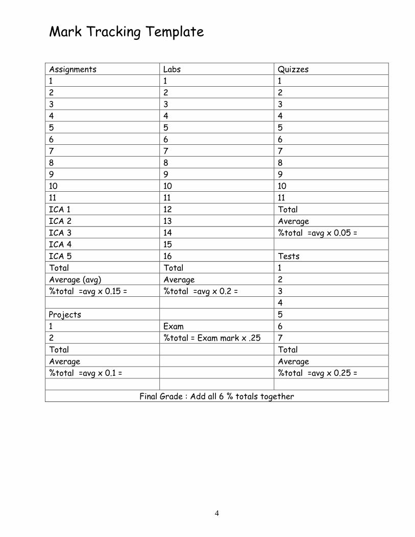
Mark Tracking Template Assignments Labs Quizzes

1 1 1

2 2 2 3 3 3

4 4 4 5 5 5

6 6 6 7 7 7

8 8 8 9 9 9

10 10 10 11 11 11

ICA 1 12 Total ICA 2 13 Average

ICA 3 14 %total =avg x 0.05 = ICA 4 15

ICA 5 16 Tests Total Total 1

Average (avg) Average 2 %total =avg x 0.15 = %total =avg x 0.2 = 3

4 Projects 5

1 Exam 6 2 %total = Exam mark x .25 7

Total Total

Average Average %total =avg x 0.1 = %total =avg x 0.25 =

Final Grade : Add all 6 % totals together

5

Physics Lab Safety Policy & Procedures

1. No “horseplay” in the lab will be tolerated. The safety of you and your classmates depends on your responsible behavior. 10 % of each lab mark is awarded for your conduct in the lab and how clean you leave your station.

2. Never perform any activity or use any lab equipment without the permission of

the teacher.

3. Report any injuries or health issues to the teacher immediately.

4. Listen to and follow all instructions given by the teacher.

5. Know the location of safety equipment – fire extinguisher, first aid kit, etc.

6. Wear appropriate clothing to the lab. Avoid long, loose clothing and jewelry.

7. Proper footwear is essential as well. Avoid sandals and high heels.

8. No food or drink is permitted in the Lab. 9. Read any written lab instructions before you come to the lab.

10. Be prepared to work as soon as you come into the lab.

11. Make sure the tables and aisles are kept free of bookbags to prevent tripping.

12. Keep the lab benches free of books, clothing and anything not needed in the lab.

13. Always use the proper tools. Us electrically insulated tools when working with

electricity.

14. Use caution when working with electrical circuits, devices, and capacitors.

15. Make sure all electrical devices are turned off and/or unplugged both before and after an experiment.

16. Make sure your lab area is clean and the chairs pushed in at the end of the

period.

6

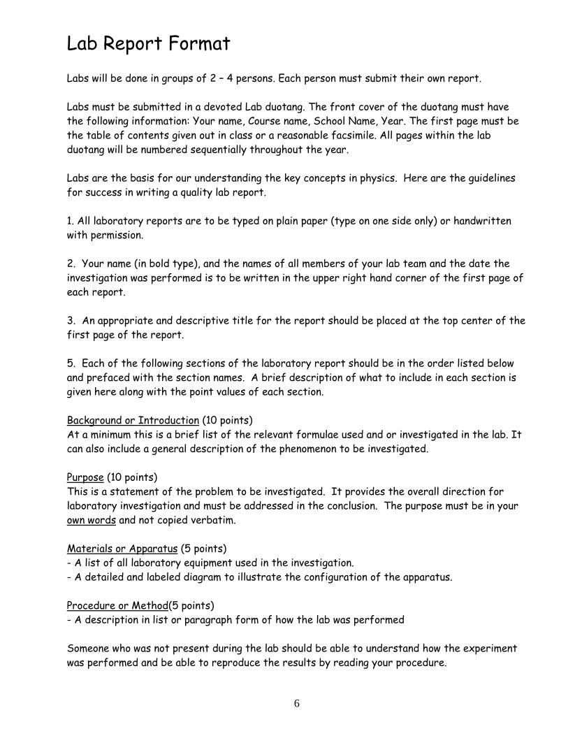
Lab Report Format Labs will be done in groups of 2 – 4 persons. Each person must submit their own report. Labs must be submitted in a devoted Lab duotang. The front cover of the duotang must have the following information: Your name, Course name, School Name, Year. The first page must be the table of contents given out in class or a reasonable facsimile. All pages within the lab duotang will be numbered sequentially throughout the year. Labs are the basis for our understanding the key concepts in physics. Here are the guidelines for success in writing a quality lab report. 1. All laboratory reports are to be typed on plain paper (type on one side only) or handwritten with permission. 2. Your name (in bold type), and the names of all members of your lab team and the date the investigation was performed is to be written in the upper right hand corner of the first page of each report. 3. An appropriate and descriptive title for the report should be placed at the top center of the first page of the report. 5. Each of the following sections of the laboratory report should be in the order listed below and prefaced with the section names. A brief description of what to include in each section is given here along with the point values of each section. Background or Introduction (10 points) At a minimum this is a brief list of the relevant formulae used and or investigated in the lab. It can also include a general description of the phenomenon to be investigated. Purpose (10 points) This is a statement of the problem to be investigated. It provides the overall direction for laboratory investigation and must be addressed in the conclusion. The purpose must be in your own words and not copied verbatim. Materials or Apparatus (5 points) - A list of all laboratory equipment used in the investigation. - A detailed and labeled diagram to illustrate the configuration of the apparatus. Procedure or Method(5 points) - A description in list or paragraph form of how the lab was performed Someone who was not present during the lab should be able to understand how the experiment was performed and be able to reproduce the results by reading your procedure.

7

- If the procedure in the Lab manual was followed, then a statement directing the marker to the appropriate location after the section title suffices.

- Any deviation from the procedure in the lab manual must be fully described in this section

Data (20 points) - Data measured directly from the experiment collected in tables with headings and gridlines are included in this section. - Derived values obtained by way of simple mathematical manipulations (for example: average values, or unit conversions) or interpretations of any kind should be included in this section of the report as well. - A sample calculation must appear showing how any calculated value was obtained. - If a calculation is repeated then its sample calculation need only be shown once. - The units for physical measurements in a data table should be specified in column headings only. Data Analysis (30 points) - Include all graphs, analysis of graphs, post laboratory calculations and percent errors. - All graphs should have a title, labeled coordinate axes and units. - All graphs should be computer generated or hand drawn on graph paper. - All lines of best fit must be drawn according to the guidelines set out on pages 16 and 17 of this manual or be computer generated. - Unusual results or trends should be noted and explained if possible. - State the meaning of the slope and discuss the significance of the y-intercept when appropriate. - Explain the possible source of any error or questionable results. - Discuss whether the goals in the purpose were achieved. - Answer all questions from the lab manual in this section - Suggest changes in experimental design which might test your explanations.

Conclusion (10 points) - State any significant numerical results with associated error. - Comparison of results with known or expected values - State whether or not the goals set out in the purpose were achieved. Lab Behaviour and Lab Report Format (10 points)

- Full marks are awarded if you work well and your lab table is tidy with the chairs on the table, equipment turned off, borrowed supplies returned, and your lab report is in the proper format in a properly formatted lab duotang.

- Marks are deducted for disruptive behaviour, careless work habits, an untidy lab table, or an incorrectly formatted lab/ lab duotang.

8

Sample Lab: Pendula Length & Period relationships

Your Name

Partner’s Name(s) Sept 10, 2007

Background: According to theory, the period of a pendulum (T) is related to

gravity (g = 9.8 m/s2) and the length of the pendulum ( l ) by the equation Purpose: To verify that the period of a pendulum is related to its length by the

equation shown above. Procedure: The pendulum was set up as shown in Figure 1-1 Figure 1-1 The mass was 1.0 kg and the displacement was 0.15 metres. These two variables remained constant throughout the entire experiment. The time to complete 20 cycles was measured using a digital stopwatch with a precision of 0.01 seconds. Three trials at each length were measured and the data was recorded in Table 1-1. The period of a single cycle was calculated by dividing the measured time by 20 as seen in Sample Calculation 1-1, and was recorded in Table 1-1. The average period was then calculated by summing the periods for each trial at that length and dividing by three as seen in Sample Calculation 1-2, and was recorded in Table 1-1.

g

lT π2=

1 cycle or period

displacement

length

mass

Rest position

9

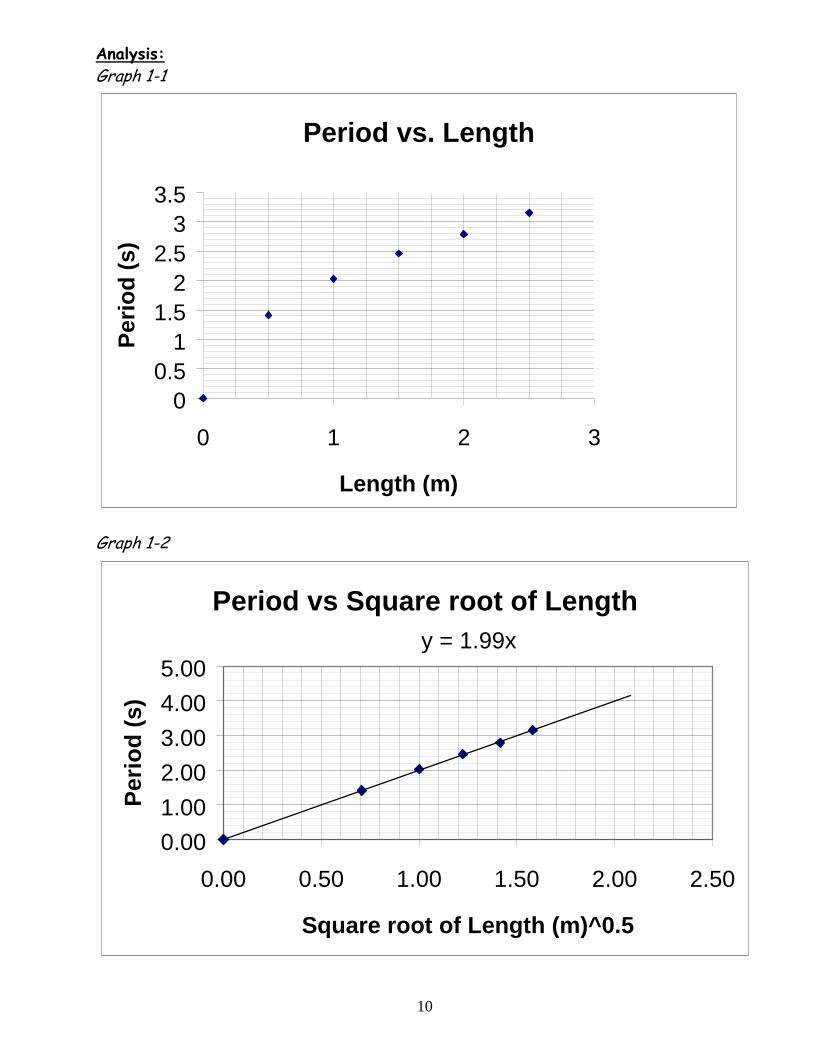
A graph of period vs. length was plotted (see Graph 1-1). A second graph was plotted of the period vs. the square root of the length and named Graph 1-2 . The slope of this line was compared to the theoretical value obtained in Sample Calculation 1-3. The percent error was calculated in Sample Calculation 1-4. Data:

Table 1-1 Length (l) (metres) ( )m

Length

Trial Time (t) for 20 cycles

(s)

Period (T) (s)

Average Period (Tave)

(s) 1 27.06 1.35

0.7071 2 29.13 1.46 0.50

3 28.90 1.41

1.41

1 43.02 2.15 1.0000 2 39.96 2.00 1.00

3 39.01 1.95

2.03

1 49.16 2.46

1.2247 2 49.97 2.50 1.50

3 48.28 2.41

2.46

1 55.73 2.79 1.4142 2 55.70 2.79 2.00

3 55.86 2.79

2.79

1 62.57 3.13

1.5811 2 63.83 3.19 2.50

3 62.42 3.12

3.15

Sample Calculation 1-1 Sample Calculation 1-2

sT

sT

tT

35.1

20/06.27

20/

===

sT

sT

sssT

TTTT

ave

ave

ave

ave

41.1

3/22.43

41.146.135.13

321

==

++=

++=

10

Analysis:

Graph 1-1

Graph 1-2

Period vs. Length

00.5

11.5

22.5

33.5

0 1 2 3

Length (m)

Per

iod

(s)

Period vs Square root of Lengthy = 1.99x

0.00

1.00

2.00

3.00

4.00

5.00

0.00 0.50 1.00 1.50 2.00 2.50

Square root of Length (m)^0.5

Per

iod

(s)

11

Analysis (cont’d)

As expected, Graph 1-1 has the approximate shape of xy = and Graph 1-2 is linear.

The slope of Graph 1-2 is less than 1% off from the expected value of g

π2. This error

is likely due to error in measuring the length of the pendulum as well as the error in measuring the period times. Sample Calculation 1-3 Sample Calculation 1-4

Conclusion Our observations agreed to within 1% that the period of a pendulum is directly related

to the square root of the length with a proportionality constant of g

π2.

lT

lT

lT

g

lT

ms

sm

sm

01.2

8.9

28.6

8.9)14.3(2

2

2

2

=

=

=

= π

%995.0%

%10000995.0%

%10001.2

99.101.2%

%100

=×=

×−=

×−

=

error

error

error

ltheoretica

ltheoreticaobservederroro

o

12

Significant Figures Significant figures (SF) are all the digits of a measurement that are certain plus one estimated digit. 56.4 mm has three significant digits. Rules for Significant Digits

1. All non zero digits are significant. 2. All final zeros after the decimal point are significant 3. Zeros between non zero digits are significant 4. Zeros used as place holders only are not significant

Example 1: 180000 has two significant digits 1 and 8 the zeros are not significant

since they are place holders Example 2: 180000.0 has 7 significant digits. The final zero is significant because

of rule 2. The other zeros are significant because of rule 3. Example 3: 0.0243 has 3 SF because the zeros are placeholders Calculations with Significant Figures

The final answer should have the same number of significant digits as the least precise number in the calculation. Examples: 12.1kg + 0.130 kg = 12.2 kg

12.5m x 16m x 15.88m = 3176m3 the least precise number (16m) has 2 s.f. so the answer should be rounded to 3200 m3.

Rounding When performing calculations, a calculator will often display many digits only a few of which are significant. These must be rounded to maintain the correct precision. Numbers within a calculation are not rounded. Rounding is only done to the final answer. Rules for rounding

1. Round down if the digits to be dropped are < 5, 50, 500 etc. 2. Round up if the digits to be dropped are > 5, 50, 500 etc. 3. Round to the even digit if the digits to be dropped are = 5, 50, 500 etc.

13

Rounding examples – each is rounded to 3 SF 125.6 = 126 125.4 = 125 125.5 = 126 124.501 = 125 124.5 = 124

Scientific Notation Scientific notation is a format used to conveniently express extremely large or small quantities. Any number can be expressed as the product of two numbers. The first factor is greater or equal to 1 and less than 10. The second factor is a power of ten. Examples: The mass of the Earth is 59 900 000 000 000 000 000 000 000 kg in standard notation. This is 5.99 x1024 kg in scientific notation. 90 kg would be 9.0x 101 kg in scientific notation. For numbers like this the only convenience is expressing the number 90 to a precision of 2 significant digits. The mass of an electron is 0.000000000000000000000000000000911 kg in standard notation. This is 9.11 x 10-31 kg in scientific notation. Only the digits in the first factor are significant. All of the digits in the first factor are significant.

Error Calculations In some of your experiments you will be required to check your results with a known value; This will be done by finding the percentage error in the experiment using the following equation: If your percentage error is less than 10% your lab can be considered a success.

%100×−

=ltheoretica

ltheoreticaobservederroro

o

14

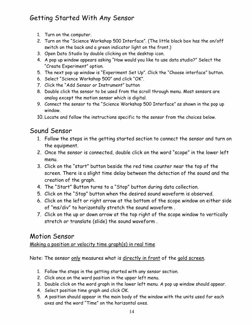
Getting Started With Any Sensor 1. Turn on the computer. 2. Turn on the “Science Workshop 500 Interface”. (The little black box has the on/off

switch on the back and a green indicator light on the front.) 3. Open Data Studio by double clicking on the desktop icon. 4. A pop up window appears asking “How would you like to use data studio?” Select the

“Create Experiment” option. 5. The next pop up window is “Experiment Set Up”. Click the “Choose interface” button. 6. Select “Science Workshop 500” and click “OK”. 7. Click the “Add Sensor or Instrument” button 8. Double click the sensor to be used from the scroll through menu. Most sensors are

analog except the motion sensor which is digital. 9. Connect the sensor to the “Science Workshop 500 Interface” as shown in the pop up

window.

10. Locate and follow the instructions specific to the sensor from the choices below.

Sound Sensor 1. Follow the steps in the getting started section to connect the sensor and turn on

the equipment. 2. Once the sensor is connected, double click on the word “scope” in the lower left

menu. 3. Click on the “start” button beside the red time counter near the top of the

screen. There is a slight time delay between the detection of the sound and the creation of the graph.

4. The “Start” Button turns to a “Stop” button during data collection. 5. Click on the “Stop” button when the desired sound waveform is observed. 6. Click on the left or right arrow at the bottom of the scope window on either side

of “ms/div” to horizontally stretch the sound waveform . 7. Click on the up or down arrow at the top right of the scope window to vertically

stretch or translate (slide) the sound waveform .

Motion Sensor Making a position or velocity time graph(s) in real time Note: The sensor only measures what is directly in front of the gold screen.

1. Follow the steps in the getting started with any sensor section. 2. Click once on the word position in the upper left menu. 3. Double click on the word graph in the lower left menu. A pop up window should appear. 4. Select position time graph and click OK. 5. A position should appear in the main body of the window with the units used for each

axes and the word “Time” on the horizontal axes.

15

6. A velocity time graph may be viewed simultaneously with the position time graph by dragging the word velocity from the upper left menu into the position time graph.

7. Start the collection of data by clicking on the start button next to the red time counter on the screen. Dots should appear on the graph and the motion sensor should be clicking away as the data is collected.

8. The Start button turns into a stop button while data is collected. Press the stop button once your data collection is complete.

Manipulating graphs.

1. The mouse pointer changes shape to indicate different options for manipulating graphs. The toolbar within the graph window gives other options.

2. Moving the mouse pointer over an axis changes the pointer to a grabbing hand which allows the movement of a graph in any direction with a click and drag.

3. Moving the mouse pointer over the numbers on an axis changes the pointer to a curly double ended arrow which allows the stretching of a graph in any direction with a click and drag.

Multiple Overlaid graphs After the first graph is created, simply press the start button again and a second graph will be created over the first. The first graph is called “Run 1” and the second graph is called “Run 2”.

Deleting a graph Select “Run 1” (or the run you would like to delete) from the upper left menu then press delete then press return or select yes from the pop up.

Creating a line of best fit

1. Select the region of the graph to be described by a line of best fit with a click and drag. (In the same manner text is selected in a word document.)

2. Click on the “Fit” button at the top middle of the graph window and select “linear fit” (or other desired graph type) from the pull down menu.

3. Delete a line of best fit in the same manner as deleting a graph. Using The “Calculate” Feature To Create a kinetic energy vs time graph from a particular velocity time graph.

1. Click on the “Calculate” button next to the red timer. 2. Enter the formula with an equals sign. Use * for times and ^ for exponents. 3. Click the “accept” button once the formula is entered. 4. To define a variable click on the down arrow next to “Please define variable”. 5. Select “data measurement” and then the run # of the data to be used. 6. Drag the Equation from the upper left data menu into the graph window. The new

Graph should appear below the original .

16

0

1

2

3

4

5

6

7

8

9

10

0 2 4 6 8 10

÷

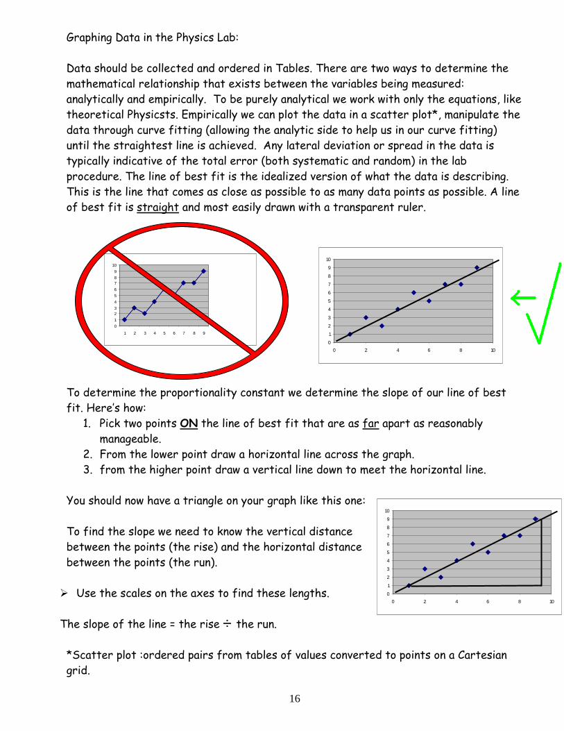
Graphing Data in the Physics Lab: Data should be collected and ordered in Tables. There are two ways to determine the mathematical relationship that exists between the variables being measured: analytically and empirically. To be purely analytical we work with only the equations, like theoretical Physicsts. Empirically we can plot the data in a scatter plot*, manipulate the data through curve fitting (allowing the analytic side to help us in our curve fitting) until the straightest line is achieved. Any lateral deviation or spread in the data is typically indicative of the total error (both systematic and random) in the lab procedure. The line of best fit is the idealized version of what the data is describing. This is the line that comes as close as possible to as many data points as possible. A line of best fit is straight and most easily drawn with a transparent ruler. To determine the proportionality constant we determine the slope of our line of best fit. Here’s how:

1. Pick two points ON the line of best fit that are as far apart as reasonably manageable.

2. From the lower point draw a horizontal line across the graph. 3. from the higher point draw a vertical line down to meet the horizontal line.

You should now have a triangle on your graph like this one: To find the slope we need to know the vertical distance between the points (the rise) and the horizontal distance between the points (the run).

� Use the scales on the axes to find these lengths. The slope of the line = the rise the run. *Scatter plot :ordered pairs from tables of values converted to points on a Cartesian grid.

0

1

23

4

5

6

78

9

10

1 2 3 4 5 6 7 8 9

0

1

2

3

4

5

6

7

8

9

10

0 2 4 6 8 10

17

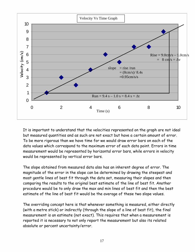
It is important to understand that the velocities represented on the graph are not ideal but measured quantities and as such are not exact but have a certain amount of error. To be more rigorous than we have time for we would draw error bars on each of the data values which correspond to the maximum error of each data point. Errors in time measurement would be represented by horizontal error bars, while errors in velocity would be represented by vertical error bars. The slope obtained from measured data also has an inherent degree of error. The magnitude of the error in the slope can be determined by drawing the steepest and most gentle lines of best fit through the data set, measuring their slopes and then comparing the results to the original best estimate of the line of best fit. Another procedure would be to only draw the max and min lines of best fit and then the best estimate of the line of best fit would be the average of these two slope values. The overriding concept here is that whenever something is measured, either directly (with a metre stick) or indirectly (through the slope of a line of best fit), the final measurement is an estimate (not exact). This requires that when a measurement is reported it is necessary to not only report the measurement but also its related absolute or percent uncertainty/error.

0

1

2

3

4

5

6

7

8

9

10

0 2 4 6 8 10

Run = 9.4 s – 1.0 s = 8.4 s = ∆t

Rise = 9.0cm/s – 1.0cm/s = 8 cm/s = ∆v

slope = rise /run = (8cm/s)/ 8.4s =0.95cm/s/s

Time (s)

Velocity Vs Time Graph

18

Lab 1: Uniform Velocity Purpose: To study uniform motion (constant velocity). To compare uniform velocity

to non uniform velocity. To gain practice in measurement of physical quantities Apparatus: Ticker timer Ticker tape (1m) Metre stick Graph paper Procedure:

1. Obtain a length of ticker tape (~1 m long). Label one end start. Pass the start end of the tape through the ticker timer.

2. Turn on the timer and pull the tape through at a constant velocity. Shut the

timer off as soon as the tape is completely through.

3. Ignore the first group of dots that are too close together to differentiate, and draw an arrow pointing to the first clear dot. This dot corresponds to time 0.00 seconds.

4. Count three spaces to the right of your starting point and mark the point at the

end of the third space. Count another three spaces and mark the point after these spaces. Continue doing this until you reach the end of your tape.

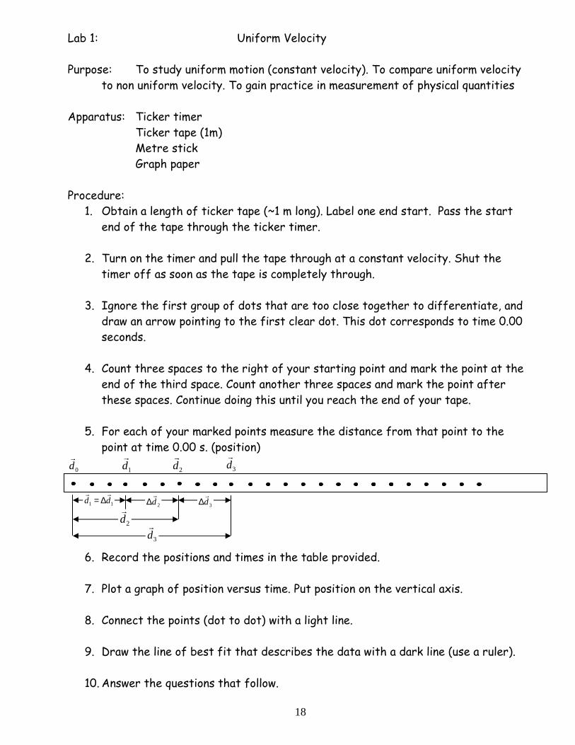
5. For each of your marked points measure the distance from that point to the

point at time 0.00 s. (position)

6. Record the positions and times in the table provided.

7. Plot a graph of position versus time. Put position on the vertical axis.

8. Connect the points (dot to dot) with a light line.

9. Draw the line of best fit that describes the data with a dark line (use a ruler).

10. Answer the questions that follow.

11 ddrr

∆=

2dr

2dr

∆ 3dr

∆

3dr

0dr

1dr

2dr

3dr

19

Data:

Time (s) Position ± (cm) 0.00 0.0

Analysis:

1. Make sure your position time graph is at least 1/2 page in size. 2. Were you able to pull the ticker timer at constant velocity? How do you know? 3. Calculate the slope of your line of best fit using two widely separated points. 4. What physical quantity does the slope of the position time graph correspond to? 5. Are there any regions of acceleration on your graph? How do you know? 6. Draw a rough position vs time graph for a motion with

a. increasing speed in + direction. b. increasing speed in - direction. c. Decreasing speed in the + direction. d. Decreasing speed in the – direction.

7. Discuss sources of error in the measurement. Estimate the precision of your measurements.

Conclusion: Address the purpose. State your approximate constant velocity with error.

Estimate approximate error here.

The ticker timer makes marks at a rate of 60 per second. What fraction of a second elapses after 30 marks? After 10 marks? After 5 marks? After 3 marks?

20

Lab 2: Measuring the Acceleration of a falling object Purpose: To determine whether or not the acceleration due to gravity is constant. If Constant, to measure this acceleration. Apparatus: Variety of masses, Ticker timer, Ticker tape, metre stick Procedure:

1. Tape a mass to the end of the ticker tape. Record The mass here: _____g 2. Insert ticker tape into the ticker timer. 3. Turn on ticker timer and allow mass to fall at the same time. 4. Choose the first clear dot as d0 at position 0.000m occurring at time t0 =0.000s. 5. Measure the position of the remaining dots with respect to d0. Record these

positions in Table T1. 6. Calculate the displacements, record these ∆d in Table T1. Show and lable one

sample calculation. 7. Calculate the velocities that correspond with each displacement. Record these

values in Table T1. Show and lable one sample calculation. 8. On one piece of graph paper make a position time graph to illustrate the motion. 9. On a separate piece of graph paper make a velocity time graph to illustrate the

motion. 10. Draw the line of best fit through the velocity/time data points. 11. Calculate the slope of the velocity time graph. Show your work on the graph.

Choose widely separated points.

Data:

See sample table on next page. Analysis:

All graphs in this section, then a discussion of your results, then these questions answered. 1. Is the d/t data what you would expect? Explain. 2. Is the v/t data linear? 3. What does the slope of the velocity time graph represent? 4. What is the % error of your slope if the expected value is 9.8 m/s2? 5. Is the acceleration due to gravity constant? Explain. 6. Identify sources of error that would make your results different than the

expected 9.8 m/s2.

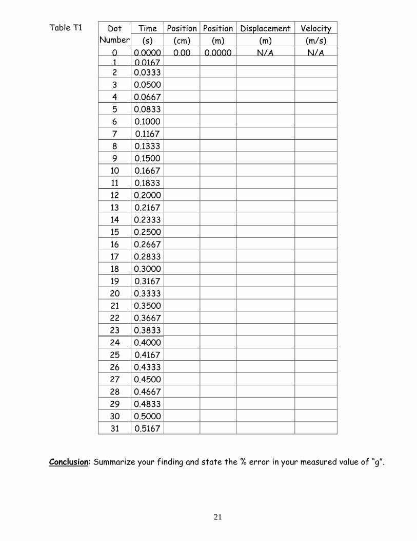
21

Table T1

Conclusion: Summarize your finding and state the % error in your measured value of “g”.

Time Position Position Displacement Velocity Dot Number (s) (cm) (m) (m) (m/s)

0 0.0000 0.00 0.0000 N/A N/A 1 0.0167 2 0.0333

3 0.0500

4 0.0667

5 0.0833

6 0.1000

7 0.1167

8 0.1333

9 0.1500

10 0.1667

11 0.1833

12 0.2000

13 0.2167

14 0.2333

15 0.2500

16 0.2667

17 0.2833

18 0.3000

19 0.3167

20 0.3333

21 0.3500

22 0.3667

23 0.3833

24 0.4000

25 0.4167

26 0.4333

27 0.4500

28 0.4667

29 0.4833

30 0.5000

31 0.5167

22

Lab 3: Uniform accelerations Purpose: To observe uniform and non uniform accelerations. To gain experience using Data Studio and Sensors. Materials: Computer with Science workshop 500 interface Motion sensor Lab cart Wooden plank Pulley string Masses Procedure:

1. Read through the sensor instructions found on pages 14-15 of this Lab Manual. 2. Connect the motion sensor and test it by recording your hand moving back and

forth in front of the sensor. 3. Record and save position/time and velocity/time graphs for the following motions:

a. A soccer ball dropped to the floor beneath a motion sensor. b. A lab cart coasting to a stop from a small speed on a lab table. c. A lab cart coasting up and then down a plank with a small incline ( 1.0≈m ). d. Two nestled basket style coffee filter dropped to the floor onto a motion

sensor. Be sure to include a descriptive title for each graph along with at least one group members name for identification if using the lab printer.

4. Use the “Fit” button to determine the accelerations associated with each motion. 5. Verify one of the slop e calculations using the method outlined on pages 16 and 17

of this manual. 6. Analyze your graphs in a paragraph or two 7. Summarize your numerical results with error estimate and address the purpose in

a conclusion.

23

Lab 4: Newton’s Second Law

Background: mgFg =r

amFFnet

rrr)(∑∑ == nxxxxx ++++=∑ ...321

Purpose: To observe how an increase of force affects the acceleration of a specific mass. Materials: Computer with Science workshop 500 Motion sensor Lab cart Pulley string Masses totaling 250 g Procedure:

1. Determine the total mass of the lab cart and masses. 2. Attach a pulley to the end of a lab bench opposite the computer. 3. Turn on the computer and connect a motion sensor. 4. Attach a 50 g mass to the end of a string and place the other masses on top of

the lab cart. 5. Record position and velocity time graphs for the motion of the lab cart pulled by

the falling mass. 6. Determine the acceleration of this motion. 7. Repeat steps 3-5 increasing the falling mass by 50 g intervals up to 250 g. 8. Collect your Data in a table Similar to the one shown here:

9. Use Newton’s second Law to predict the acceleration the Lab cart will experience with each falling mass.

10. Discuss your results in a paragraph or two and determine the percent difference between the predicted and observed accelerations.

11. Organize your work into a formal Lab report.

Falling Mass

Force Provided

(N)

Acceleration of system (observed)

(m/s2)

Acceleration of system (predicted)

(m/s2)

50 g 100 g

150 g 200 g

250 g

mass

24

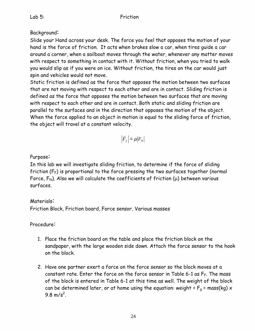
Lab 5: Friction

Background: Slide your Hand across your desk. The force you feel that opposes the motion of your hand is the force of friction. It acts when brakes slow a car, when tires guide a car around a corner, when a sailboat moves through the water, whenever any matter moves with respect to something in contact with it. Without friction, when you tried to walk you would slip as if you were on ice. Without friction, the tires on the car would just spin and vehicles would not move. Static friction is defined as the force that opposes the motion between two surfaces that are not moving with respect to each other and are in contact. Sliding friction is defined as the force that opposes the motion between two surfaces that are moving with respect to each other and are in contact. Both static and sliding friction are parallel to the surfaces and in the direction that opposes the motion of the object. When the force applied to an object in motion is equal to the sliding force of friction, the object will travel at a constant velocity.

Nf FF µ=r

Purpose: In this lab we will investigate sliding friction, to determine if the force of sliding friction (FF) is proportional to the force pressing the two surfaces together (normal Force, FN). Also we will calculate the coefficients of friction (µ) between various surfaces.

Materials: Friction Block, Friction board, Force sensor, Various masses

Procedure:

1. Place the friction board on the table and place the friction block on the sandpaper, with the large wooden side down. Attach the force sensor to the hook on the block.

2. Have one partner exert a force on the force sensor so the block moves at a

constant rate. Enter the force on the force sensor in Table 6-1 as FF. The mass of the block is entered in Table 6-1 at this time as well. The weight of the block can be determined later, or at home using the equation: weight = Fg = mass(kg) x 9.8 m/s2.

25

3. Repeat steps 1 & 2 increasing the mass by even increments (if possible) until there are 10 rows of data in Table 6-1 (wood/sandpaper interface).

4. Repeat steps 1 to 3 using the same block on the metal surface. Record your data

in table 6-2 (wood/metal interface). 5. Repeat steps 1 to 3 with a different surface/surface interface. Enter the data in

Table 6-3 and indicate the surfaces you have chosen.

Sample Tables Only: (one row for each weight pulled) Table 6-1 Wood and Sandpaper Table 6-2 Wood and Metal Table 6-4 Coefficients of Friction

Questions to include in Analysis section:

1. Calculate the weights and determine the normal forces to complete your data tables.

2. For each data table, plot a scatterplot of the force of friction vs the Normal force for each data set. (Normal force on horizontal axis)

3. Draw the line of best fit for each data set. How well does the line of best fit describe your data?

4. What does the slope of each best fit line represent? 5. Record the coefficients of friction and the surface types in table 6-4. 6. Discuss your results in a paragraph. Do they make sense? Are they what you

expected? Organize your work into a formal Lab report.

Mass of Block (kg)

Weight of Block (N)

Normal force (N)

Frictional force (N) ±

Mass of Block (kg)

Weight of Block (N)

Normal force (N)

Frictional force (N) ±

Surface Types µ

/

26

Lab 6: Hooke’s Law

Background: kxFs −=r

mgFg =r

Purpose: To determine the spring constant of a large spring. To determine how well Hooke’s law describes the big spring’s in the physics Lab. Materials: Big Spring Bathroom scale Metre stick Procedure:

1. Use one of the springs hanging from the ceiling. 2. Determine the spring constant of the spring by hanging a known mass from the

end of the spring (you), measuring the amount of stretch and plugging these values into the Hooke’s Law Formula.

3. Place other group members on the end of the spring (one at a time) and measure the stretch each time.

4. Measure the stretch that corresponds to 0 kg, 5 kg, 10 kg and so on in 5kg increments up to 70kg hanging from the end of the spring. (Hint: with your feet on the bathroom scale while you are sitting on the end of the spring, gradually transfer your weight from the bathroom scale to the spring.

5. Produce a F vs x data table and graph. 6. Compare the slope of the graph to your k value found in step 2. 7. Discuss your results in a paragraph. 8. Summarize your k value with estimated error in a sentence or two in a conclusion.

27

Lab 7: Conservation of Momentum Background: ∑ ∑ ′= pp

Purpose: To determine how well the conservation of momentum describes an elastic collision between two lab Carts Materials: Computer with interface Motion sensors (x2) Lab carts (x2) Procedure:

1. Working with an adjacent group, set up a head on collision between 2 lab carts. 1 group records the motion of 1 lab cart, the other group records the motion of the other lab cart.

2. Produce a velocity time graph for each of the carts in each of the following collisions. (Data Section)

a. Carts of equal masses moving towards each other with equal speed. b. Carts of equal masses one stationary and one moving. c. Carts of unequal masses (by 1 kg or more) repeating the “a” and “b” cases.

3. Determine the total momentum of the systems both before and after the collisions. (Analysis section)

4. Determine the % error of the observations. 5. Organize your work into a formal lab report.

28

Lab 8: Work, Energy & Power Lab

Background: ||W F d= ∆ t

WP

∆= gE mgh= W E= ∆

Purpose: To develop your understanding of work, energy and power. To calculate your own power output capabilities. Apparatus: Stopwatch or timing device Measuring tape Bathroom Scale Procedure:

1. Obtain a measurement for the change in height between ground level and the third floor.

2. Obtain a measurement for your mass. 3. Measure the amount of time it takes to walk up the stairs at a “normal” speed. 4. Repeat step three for a slower pace. 5. Repeat step three for your fastest safe pace. 6. Enter the data in table T-1 7. Answer the questions that follow.

Data: My mass: _____±___kg My weight:____±___N Staircase height: ____±__m

Speed FApplied

± (N) Displacement

± (m) Work

± ( j) Time

± (s) Power

± (w) Power

(Horsepower) Slow

Normal Fastest

Analysis:

1. Analyze your motion up the stairs in a brief paragraph: Think in terms of constant velocity, acceleration, and whether the motion is truly 1 dimensional.

2. What amount of work is done when moving in these other dimensions?

3. What does the || symbol next to the force variable in dFWrr

∆= || mean?

4. How much does your gravitational potential energy change by climbing the stairs? 5. Does your speed up the stairs affect the change in gravitational potential

energy? 6. What affects the power output? How can you maximize your power? Minimize? 7. Which quantity had the greatest % error associated with its measurement?

Organize your work in a formal lab report.

Unit Conversions: 0.454kg = 1.0 lb 2.2 lbs = 1.0 kg

746 watts = 1 horsepower

29

Lab 9: Conservation of Energy

Background: ∑ ∑ ′= EE 2

2

1mvEk = mghEg =

Purpose: To examine the transfer of energy and the conservation of energy for a cart rolling up and down a ramp. Materials: Computer with sensors Lab cart Inclined Plank Procedure:

1. Measure as precisely as possible the angle of the incline (Very important!) 2. Record the motion of a cart rolling freely up and then back down the incline. 3. Use the calculate feature of Data Studio to produce the following graphs from

position and velocity time graphs in step one. a. Kinetic energy - b. Gravitational energy c. Total energy

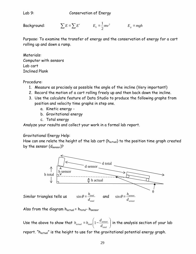
Analyze your results and collect your work in a formal lab report. Gravitational Energy Help: How can one relate the height of the lab cart (hactual) to the position time graph created by the sensor (dsensor)?

Similar triangles tells us total

total

d

h=θsin and sensor

sensor

d

h=θsin

Also from the diagram hactual = htotal- hsensor

Use the above to show that

−=

total

sensortotalactual d

dhh 1 in the analysis section of your lab

report. “hactual” is the height to use for the gravitational potential energy graph.

θ

h total

d total d sensor

h actual

h sensor

30

Lab 10: Pulleys, Work and Energy In this lab we are going to lift a 1.00 kg mass a distance of 0.10 m at 6 different stations. Each station has a different set of pulleys. THE PULLEYS ARE VERY DELICATE AND WILL BECOME TANGLED IF USED IMPROPERLY. EXTREME CARE MUST BE EXERCISED WHEN OPERATING THEPULLEYS. DELIBERATE MISUSE WILL RESULT IN REMOVAL FROM THE LAB AND A MARK OF ZERO FOR THE LAB. Start by calculating the change in gravitational potential energy of a 1.00 kg mass if you lift it 10 cm. Enter this value in your table. Will this value change or be the same for each set of pulleys? To lift the mass you must apply a force to the string. Use the force sesnsor to measure the force required to lift the mass at a constant slow rate. This value is FApplied. Use the meter stick to measure the distance you have to pull (d) in order to lift the mass 10 cm. You may mark the string with pen or marker if you like. Calculate the Work required to lift the mass 10 cm and enter this value in your table.

Station Number of strings

supporting mass

∆E of 1.00kg

mass (J)

FApplied (N)

D pulled (m)

Work (J)

1a (no pulley) 1b 2 3 4 5 6

Questions to address in Analysis Section

1. How does the FApplied vary with respect to the number of strings supporting the mass? Describe the pattern in the simplest terms possible.

2. Is the change in energy for each station the same or different? Why? 3. Is the amount of work required at each station the same or different? Why? 4. Estimate the precision of each measured quantity.

31

Lab 11: Vibration of a Long Spring and Wave Speed With the long spring used before stretched to 4.905 m (16 floor tiles) send an individual pulse down the 7m spring and determine the speed of this pulse. Record the speed and how it was obtained. Next, practice setting up each of the standing waves in the table below. Once you are able to consistently make each of the standing wave patterns use a stopwatch to time 20 complete cycles. Do this 2 or three times for each harmonic then calculate the average for each in the table.

1. Calculate the frequency of each mode of vibration based on the average time. 2. Do your observations agree with the theory presented in class? (For the 1st

harmonic 0ff = , for the 2nd harmonic 02 ff = ,for the 3rd harmonic 03 ff = , and

for the 4th harmonic 04 ff = )

3. Determine the wavelength of each wave in metres. (The 1st harmonic is λ21 , the

2nd harmonic is λ1 , the 3rd harmonic is λ23 , and the 4th harmonic is λ2 )

4. If you multiplied units of frequency by units of wavelength what units do you get? 5. Perform the numerical calculation in question 4 for each of the harmonics. 6. Compare the speed of an individual pulse to your results from question 5.

Picture of Standing Wave

Name Structure Times for 20 Cycles

Freq

(Hz)

Wave length (m)

1st Harmonic or

Fundamental

1 Antinode

2 Nodes

2nd Harmonic or 1st

Overtone

2 Antinodes

3 Nodes

3rd Harmonic or 2nd

Overtone

3 Antinodes

4 Nodes

4th Harmonic or 3rd

Overtone

4 Antinodes

5 Nodes

32

Lab 12: Sound Waves Background: Sound is a longitudinal vibration of the air that travels in all directions from a source of vibration. The frequency of a sound is equal to the frequency of the vibration which created the sound and is related to the pitch that we hear. The loudness of a sound is related to the amplitude of the vibration. Caution: Never strike a tuning fork against anything hard like a desk or other

tuning fork. This will permanently damage the tuning fork. To sound a tuning fork,

hold the base and strike it against your knee, knuckle, flick it with your fingernail

or use a proper tuning fork hammer

T

f1= 12 fffbeat −=

n

n wavesfor time=T ∑= AAtotal

Purpose: To determine the fundamental frequency of a tuning fork and compare it to its expected value. To determine the overtone frequency of a damaged tuning fork. To determine the beat frequency produced between two similar tuning forks. Materials: Computer with sound sensor Two similar tuning forks Procedure:

1. Read the sound sensor instructions on page 14 of this Lab Manual. 2. Turn on the computer and connect the sound sensor. 3. Strike one tuning fork on your knee. Document in writing what it sounds like to

the unaided ear, record the sound and save the scope display from Data Studio. 4. Repeat step 3 for the other tuning fork. 5. Determine the frequency of each by counting the number of waves that occur in a

certain amount of time. Note: time is on the horizontal axis. 6. Calculate the percent difference between the observed frequencies and the

frequencies printed on the tuning fork. 7. Record the sound produced by flicking one of the tuning forks with a fingernail. 8. Document in writing what it sounds like to the unaided ear, record the sound and

save the scope display from Data Studio. 9. Determine the frequency of the low and the high tone separately. 10. Strike both tuning forks against your knee(s) at the same time. 11. Document in writing what it sounds like to the unaided ear, record the sound and

save the scope display from Data Studio. 12. Compare your observations with the expected beat frequency and determine the

% error.

33

Lab 13: Speed of sound

Background: λfv = 4

)12(λ−= nLn

Tf

1=

Purpose: To measure resonant lengths of a closed end vibrating air column. To determine the frequency, wavelength and speed of sound produced by a tuning fork. Materials: 1-2 litre graduated cylinder 1 ½” pvc pipe as tall as the graduated cylinder Metre stick 1024 Hz Tuning Fork Room temperature water Thermometer Procedure:

1. Place the1 ½” pvc pipe into the graduated cylinder. 2. Fill the cylinder with the room temperature water. 3. Record the room temperature. 4. Sound the tuning fork against your knee and hold it over the open end of the pvc

pipe. 5. Raise the pipe slowly out of the water while keeping the tuning fork positioned

over the end of the pvc pipe. 6. Locate the positions for which the sound increases dramatically. Ignore the

positions of slightly increased sound caused by resonance with the damage overtones.

7. Measure the Height of the vibrating air column inside the pvc pipe (from the water surface to the top of the pipe) for each of the resonant lengths.

8. Create a table with the following column headings: Resonant Number

(n) 2n-1 Resonant length (m) 4x Resonant Length

(m)

9. Record the data from step 7 in this table. 10. Create a graph with 4L on the vertical axis against (2n-1) on the horizontal axis. 11. Draw the line of best fit and determine the slope. 12. What does the slope of the graph represent? Hint: consider the central formula

from the Background above. 13. Measure the frequency of the tuning fork as done in Lab 12. 14. Determine the speed of sound in the lab based on v = fλ 15. Compare this to the expected speed of sound at room temperature. 16. Determine the percent difference between the speeds from steps 14 and 15.

34

Lab 14: Refraction of light Background: The index of refraction of a medium is the ratio of the speed of light in a vacuum to the speed of light in that medium. When light is incident on a boundary between two media it changes direction (is refracted) as it enters the new media. The amount of refraction depends on the indices of refraction of the two media and is described by Snell’s law.

v

cn = rrii nn θθ sinsin =

1

2sinn

nc =θ

Purpose: To verify Snell’s Law. To determine the index of refraction of a semicircular acrylic prism. To measure the critical angle and observe total internal reflection. Materials: Laser pointer semicircular acrylic prism Polar Graph paper Protractor Procedure:

1. Place the prism on the centre of the polar graph paper with the flat face aligned with the 0 – 180˚ line.

2. Shine the laser along the 90˚ line and ensure that the ray exits along the 270˚ line. This checks the alignment of the prism.

3. Shine the Laser along the line that is 5˚ off the Normal. Record the angle of incidence and the angle of refraction in a table.

4. Repeat Step 3 changing the angle of incidence by 5 degree increments from 0 to 90˚ with respect to the normal.

5. Create a new table with Headings iθsin and rθsin .

6. Plot iθ against rθ on a scatterplot. ( rθ on horizontal axis)

7. Plot iθsin against rθsin on a scatterplot. ( rθsin on horizontal axis)

8. Draw the line of best fit on the graph from step 7 and determine the slope. 9. What does the slope represent? 10. Determine the critical angle for total internal reflection based on this value. 11. Measure the critical angle for total internal reflection. 12. Calculate the percent error of your found index of refraction assuming 1.54 to be

the actual value. 13. Calculate the percent difference between your calculated and observed critical

angle. 14. Determine the speed of light in acrylic.

CAUTION: NEVER SHINE A LASER INTO YOUR EYES. THIS COULD CAUSE PERMANENT EYE DAMAGE.

35

Lab 15: Lenses Background: In Lab 14, you observed the phenomenon of refraction for a semicircular piece of acrylic. The bending or refraction of the light was observed for two interfaces, one from air to acrylic, and the other from acrylic to air. Recall that the amount of refraction depends on both the angle of incidence and the change in index of refraction at the interface (Snell's law). Recall the semicircular shape was chosen to allow for refraction to occur at the flat interface only since the refracted ray exited the prism along the normal. Refraction will occur for shapes of other kinds as well. A particularly interesting shape is the shape of a lens. There are two specific general lens shapes that have many practical uses. One of these shapes is where the glass bows inwards toward the center of the lens. This is a so-called “concave” shape. The other notable shape is where the glass bows outwards from the lens center. This is a so-called “convex” shape.

With a convex lens, the surface of the refracting material (glass typically) is

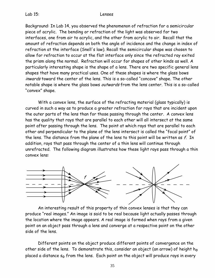
curved in such a way as to produce a greater refraction for rays that are incident upon the outer parts of the lens than for those passing through the center. A convex lens has the quality that rays that are parallel to each other will all intersect at the same point after passing through the lens. The point at which rays that are parallel to each other and perpendicular to the plane of the lens intersect is called the “focal point” of the lens. The distance from the plane of the lens to this point will be written as f. In addition, rays that pass through the center of a thin lens will continue through unrefracted. The following diagram illustrates how these light rays pass through a thin convex lens:

F

An interesting result of this property of thin convex lenses is that they can

produce “real images.” An image is said to be real because light actually passes through the location where the image appears. A real image is formed when rays from a given point on an object pass through a lens and converge at a respective point on the other side of the lens.

Different points on the object produce different points of convergence on the

other side of the lens. To demonstrate this, consider an object (an arrow) of height ho

placed a distance so from the lens. Each point on the object will produce rays in every

f

36

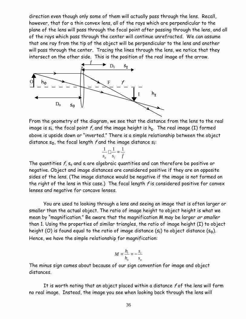
direction even though only some of them will actually pass through the lens. Recall, however, that for a thin convex lens, all of the rays which are perpendicular to the plane of the lens will pass through the focal point after passing through the lens, and all of the rays which pass through the center will continue unrefracted. We can assume that one ray from the tip of the object will be perpendicular to the lens and another will pass through the center. Tracing the lines through the lens, we notice that they intersect on the other side. This is the position of the real image of the arrow.

f

D

D

F

I

O

o

i

From the geometry of the diagram, we see that the distance from the lens to the real image is si, the focal point f, and the image height is hI. The real image (I) formed

above is upside down or “inverted.” There is a simple relationship between the object distance so, the focal length f and the image distance si:

fss io

111 =+

The quantities f, so and si are algebraic quantities and can therefore be positive or negative. Object and image distances are considered positive if they are on opposite sides of the lens. (The image distance would be negative if the image is not formed on the right of the lens in this case.) The focal length f is considered positive for convex lenses and negative for concave lenses.

You are used to looking through a lens and seeing an image that is often larger or

smaller than the actual object. The ratio of image height to object height is what we mean by “magnification.” Be aware that the magnification M may be larger or smaller than 1. Using the properties of similar triangles, the ratio of image height (I) to object height (O) is found equal to the ratio of image distance (si) to object distance (so).

Hence, we have the simple relationship for magnification:

o

i

o

i

s

s

h

hM −==

The minus sign comes about because of our sign convention for image and object distances.

It is worth noting that an object placed within a distance f of the lens will form no real image. Instead, the image you see when looking back through the lens will

ho

hI

so

sI

f

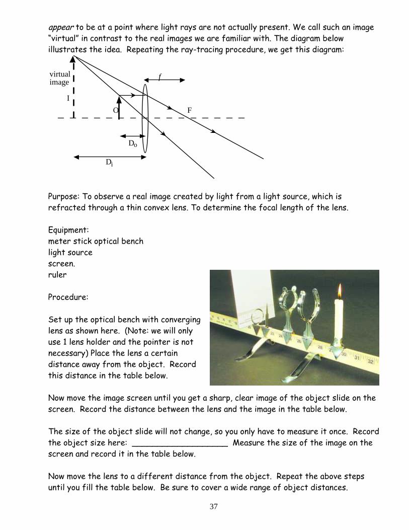
37

appear to be at a point where light rays are not actually present. We call such an image “virtual” in contrast to the real images we are familiar with. The diagram below illustrates the idea. Repeating the ray-tracing procedure, we get this diagram:

f

D

D

F

I

O

o

i

virtual image

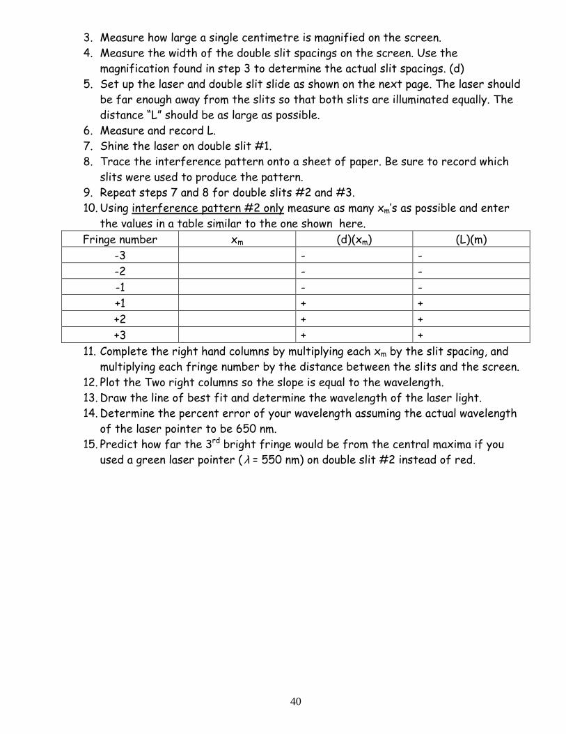
Purpose: To observe a real image created by light from a light source, which is refracted through a thin convex lens. To determine the focal length of the lens. Equipment: meter stick optical bench light source screen. ruler Procedure: Set up the optical bench with converging lens as shown here. (Note: we will only use 1 lens holder and the pointer is not necessary) Place the lens a certain distance away from the object. Record this distance in the table below. Now move the image screen until you get a sharp, clear image of the object slide on the screen. Record the distance between the lens and the image in the table below. The size of the object slide will not change, so you only have to measure it once. Record the object size here: ___________________ Measure the size of the image on the screen and record it in the table below. Now move the lens to a different distance from the object. Repeat the above steps until you fill the table below. Be sure to cover a wide range of object distances.

38

Object distance

Image distance Image size Focal length Magnification

Are there any object distances for which you cannot get a clear image? What can you determine about the lens from this information? Determine the focal length of this lens for each of the image distances. Enter these values in the table above. Draw a graph of object distance vs. image distance. What conclusions can you draw about the relationship between object distance and image distance? Determine the magnification for each of your data points. Can you find a relationship between magnification and any of your other data? Make a data table and then graph of 1/si vs 1/so (1/si on the vertical axis). Draw the line of best fit through the data points. Bonus: Determine the focal length of the lens based on the graph.

39

Lab 16: Young’s Double Slit Experiment Background:

d

Lmxm

λ≈

(on wall) Purpose: To determine the wavelength of the light from a laser pointer Materials: Laser pointer and holder Double slit slide and holder Transparent ruler Overhead projector and screen Metre stick 10 metre measuring tape Procedure:

1. Ensure your laser is working Place the double slit slide on the overhead projector with the transparent ruler.

2. Turn the projector on and focus the image on the screen

mx - The distance from the central bright fringe to the centre of

the mth bright fringe. m - The integer number of fringes from the central bright fringe λ - The wavelength of monochromatic light. L – The distance from the screen to the slits. d – The distance between the slits.

Slits # 1

Slits # 2

Slits # 3

m values -3 -2 -1 0 +1 +2 +3

x(-3) x(+2) L

Laser

d

Interference Pattern

40

3. Measure how large a single centimetre is magnified on the screen. 4. Measure the width of the double slit spacings on the screen. Use the

magnification found in step 3 to determine the actual slit spacings. (d) 5. Set up the laser and double slit slide as shown on the next page. The laser should

be far enough away from the slits so that both slits are illuminated equally. The distance “L” should be as large as possible.

6. Measure and record L. 7. Shine the laser on double slit #1. 8. Trace the interference pattern onto a sheet of paper. Be sure to record which

slits were used to produce the pattern. 9. Repeat steps 7 and 8 for double slits #2 and #3. 10. Using interference pattern #2 only measure as many xm’s as possible and enter

the values in a table similar to the one shown here. Fringe number xm (d)(xm) (L)(m)

-3 - - -2 - -

-1 - - +1 + +

+2 + + +3 + +

11. Complete the right hand columns by multiplying each xm by the slit spacing, and multiplying each fringe number by the distance between the slits and the screen.

12. Plot the Two right columns so the slope is equal to the wavelength. 13. Draw the line of best fit and determine the wavelength of the laser light. 14. Determine the percent error of your wavelength assuming the actual wavelength

of the laser pointer to be 650 nm. 15. Predict how far the 3rd bright fringe would be from the central maxima if you

used a green laser pointer (λ = 550 nm) on double slit #2 instead of red.

41