COPPE/UFRJ

ALGORITMOS POLINOMIAIS PARA PROBLEMAS DE OTIMIZACAO

COMBINATORIA COM MULTI-OBJETIVOS EM GRAFOS

Leizer de Lima Pinto

Tese de Doutorado apresentada ao Programa

de Pos-graduacao em Engenharia de

Sistemas e Computacao, COPPE, da

Universidade Federal do Rio de Janeiro,

como parte dos requisitos necessarios a

obtencao do tıtulo de Doutor em Engenharia

de Sistemas e Computacao.

Orientador: Nelson Maculan Filho

Rio de Janeiro

Dezembro de 2009

ALGORITMOS POLINOMIAIS PARA PROBLEMAS DE OTIMIZACAO

COMBINATORIA COM MULTI-OBJETIVOS EM GRAFOS

Leizer de Lima Pinto

TESE SUBMETIDA AO CORPO DOCENTE DO INSTITUTO ALBERTO LUIZ

COIMBRA DE POS-GRADUACAO E PESQUISA DE ENGENHARIA (COPPE)

DA UNIVERSIDADE FEDERAL DO RIO DE JANEIRO COMO PARTE DOS

REQUISITOS NECESSARIOS PARA A OBTENCAO DO GRAU DE DOUTOR

EM CIENCIAS EM ENGENHARIA DE SISTEMAS E COMPUTACAO.

Examinada por:

Prof. Nelson Maculan Filho, D. Habil.

Prof. Claudio Thomas Bornstein, Dr. Rer. Nat.

Prof. Paolo Toth, Ph.D.

Profa. Celina Miraglia Herrera de Figueiredo, D.Sc.

Prof. Abilio Pereira de Lucena Filho, Ph.D.

Profa. Nair Maria Maia de Abreu, D.Sc.

Prof. Geraldo Robson Mateus, D.Sc.

RIO DE JANEIRO, RJ – BRASIL

DEZEMBRO DE 2009

Pinto, Leizer de Lima

Algoritmos polinomiais para problemas de otimizacao

combinatoria com multi-objetivos em grafos/Leizer de

Lima Pinto. – Rio de Janeiro: UFRJ/COPPE, 2009.

IX, 77 p. 29, 7cm.

Orientador: Nelson Maculan Filho

Tese (doutorado) – UFRJ/COPPE/Programa de

Engenharia de Sistemas e Computacao, 2009.

Referencias Bibliograficas: p. 29 – 33.

1. Problemas Multi-Objetivo. 2. Funcoes Gargalo.

3. Solucao Pareto-Otima. I. Maculan Filho, Nelson.

II. Universidade Federal do Rio de Janeiro, COPPE,

Programa de Engenharia de Sistemas e Computacao. III.

Tıtulo.

iii

Ao meu avo Benigno

( in memoriam).

iv

Agradecimentos

Primeiramente agradeco a Deus pela minha existencia e pelos orientadores aten-

ciosos, respeitosos e eticos que tive nesta minha caminhada; aos Professores Claudio

Bornstein e Nelson Maculan que me proporcionaram um otimo ambiente de tra-

balho, pela orientacao, ensinamento, atencao, compreensao e pelo apoio de sempre;

aos Professores Celina Figueiredo, Nair Abreu, Abilio Lucena, Geraldo Mateus e

Paolo Toth por terem aceito participar desta avaliacao; ao Professor Gilbert Laporte

da HEC/Universidade de Montreal pela presteza e atencao durante o perıodo em

que estive no CIRRELT (de janeiro a julho de 2009), e pelo trabalho em conjunto no

desenvolvimento do algoritmo para um problema tri-objetivo de arvore de Steiner, o

qual compoe parte desta tese; a Professora Marta Pascoal do INESC/Universidade

de Coimbra pelas nossas discussoes, em janeiro de 2009 no CIRRELT, que resul-

taram nos algoritmos Escada e Blocos para um problema de caminho tri-objetivo,

os quais tambem compoem parte desta tese; ao Professor Marco Antonio da Univer-

sidade Catolica de Goias pelos ensinamentos durante os anos de iniciacao cientıfica,

os quais foram fundamentais para os meus estudos aqui na COPPE; ao meu amigo

e irmao (de coracao) Elivelton, pela amizade ao longo destes anos, pela contribuicao

no meu ingresso aqui na COPPE, e pela recepcao e companhia em Montreal; aos

companheiros do G4 e grandes amigos, Fabio, Jesus e Vinıcius, que estao sempre

prontos para ajudar, pelos seminarios, pelo futebol e pelos varios momentos de

descontracao; a Fatima, a Taısa e a todas as secretarias do PESC pela ajuda de

sempre; a minha mae, ao meu pai, a minha irma e ao meu sobrinho Fellipe pelo

amor, carinho e por compreenderem minha ausencia em momentos importantes de

suas vidas; as minhas tias, tios, primas e primos que, mesmo distantes, estao sem-

pre torcendo pelas minhas conquistas; ao amigo Dr Siguero Taia pela motivacao

de sempre e pela agradavel pescaria no rio Araguaia em agosto de 2009; aos meus

v

amigos da minha cidade natal, Itaguaru-GO, que sempre me recebem tao bem; ao

Conselho Nacional de Desenvolvimento Cientıfico e Tecnologico do Brasil (CNPq)

pelo suporte financeiro.

vi

Resumo da Tese apresentada a COPPE/UFRJ como parte dos requisitos necessarios

para a obtencao do grau de Doutor em Ciencias (D.Sc.)

ALGORITMOS POLINOMIAIS PARA PROBLEMAS DE OTIMIZACAO

COMBINATORIA COM MULTI-OBJETIVOS EM GRAFOS

Leizer de Lima Pinto

Dezembro/2009

Orientador: Nelson Maculan Filho

Programa: Engenharia de Sistemas e Computacao

O foco deste trabalho sao problemas de otimizacao combinatoria multi-objetivo

em grafos considerando, no maximo, uma funcao totalizadora (por exemplo, Min-

Sum ou MaxProd). As demais funcoes objetivo consideradas sao do tipo gargalo

(MinMax ou MaxMin). Algoritmos polinomiais para a obtencao de um conjunto

mınimo completo de solucoes Pareto-otimas serao apresentados, juntamente com

demonstracoes de otimalidade, experimentos computacionais e aplicacoes para o

caso tri-objetivo. Em particular, arvore geradora, arvore de Steiner e caminho sao

os problemas considerados nesta tese.

vii

Abstract of Thesis presented to COPPE/UFRJ as a partial fulfillment of the

requirements for the degree of Doctor of Science (D.Sc.)

POLYNOMIAL ALGORITHMS FOR MULTI-OBJECTIVE COMBINATORIAL

OPTIMIZATION PROBLEMS IN GRAPHS

Leizer de Lima Pinto

December/2009

Advisor: Nelson Maculan Filho

Department: Systems Engineering and Computer Science

The focus of this work are multi-objective combinatorial optimization problems

in graphs with at most one totalizing objective function (for example, MinSum or

MaxProd). The other objectives are of the bottleneck type (MinMax or MaxMin).

Polynomial algorithms are developed which generate a minimal complete set of

Pareto-optimal solutions. Optimality proofs, computational experiments and appli-

cations for tri-objective cases are given. In particular, spanning tree, Steiner tree

and optimal paths problems are considered.

viii

Sumario

1 Introducao e Revisao Bibliografica 1

2 Problemas 5

2.1 Um modelo multi-objetivo para caminhos e arvore geradora . . . . . 5

2.2 Um problema de arvore de Steiner . . . . . . . . . . . . . . . . . . . . 8

2.3 Aplicacoes . . . . . . . . . . . . . . . . . . . . . . . . . . . . . . . . . 9

2.3.1 Um problema de transporte . . . . . . . . . . . . . . . . . . . 9

2.3.2 Uma rede de sensores . . . . . . . . . . . . . . . . . . . . . . . 10

2.3.3 Uma rede de telecomunicacoes . . . . . . . . . . . . . . . . . . 11

3 Algoritmos para problemas de caminho tri-objetivo 12

4 Um algoritmo para um problema de Steiner 15

5 Algoritmos multi-objetivo 17

5.1 Algoritmo MMS-B generalizado . . . . . . . . . . . . . . . . . . . . . 18

5.2 Resultados computacionais . . . . . . . . . . . . . . . . . . . . . . . . 22

6 Consideracoes finais 26

Referencias Bibliograficas 29

Anexo 1 34

Anexo 2 44

Anexo 3 58

Anexo 4 69

ix

Capıtulo 1

Introducao e Revisao Bibliografica

Nesta tese estamos interessados em problemas de Otimizacao Combinatoria

Multi-objetivo em Grafos (OCMG). Algoritmos polinomiais para estes problemas

serao apresentados, que sao os resultados principais deste trabalho.

Na resolucao de problemas mono-objetivo a meta principal e a obtencao de uma

solucao otima. Algoritmos para problemas de caminho e de arvore geradora sao

apresentados em Ahuja et al [1]. Um software didatico para oito problemas de

caminho mono-objetivo incluindo MinSum, MinMax e MaxProd e apresentado em

Pinto e Bornstein [26], contendo implementacoes dos algoritmos de Dijkstra [11] e

de atualizacao de distancias (veja, por exemplo, Bellman [3]).

Em problemas multi-objetivo a ideia de solucao otima e substituıda pela ideia

de solucao Pareto-otima (tambem podemos dizer solucao eficiente ou solucao nao

dominada) e o interesse e obter um conjunto mınimo (ou maximo) completo de

solucoes Pareto-otimas.

As primeiras definicoes de dominancia e solucao Pareto-otima surgiram em 1896

com Pareto [24]. O primeiro trabalho na area da Pesquisa Operacional (PO) uti-

lizando esses conceitos foi apresentado por Koopmans [21] em 1951. Esses conceitos

sao fundamentais no campo da Programacao multi-objetivo, que e estudada em

diversas areas da PO, por exemplo em Programacao Linear (veja Zeleny [39]).

Normalmente, dois tipos de funcoes objetivo sao consideradas na literatura de

1

OCMG: soma e gargalo. Estas funcoes avaliam as solucoes atraves da soma dos

pesos de seus elementos (MinSum) e pelo pior peso de seus elementos (MinMax

ou MaxMin), respectivamente. Denominamos essas funcoes que envolvem todos

os elementos da solucao, como as do tipo soma, de funcoes totalizadoras. A funcao

MaxProd, que consiste em maximizar o produto dos pesos dos elementos da solucao,

e um outro exemplo de funcao totalizadora. Ehrgott e Gandibleux [12] apresentam

mais de duzentas referencias em otimizacao combinatoria multi-objetivo.

Hansen [18], Martins [23] e Berman et al [4] apresentam algoritmos polinomiais

para o problema de caminho bi-objetivo com uma funcao totalizadora e outra de

gargalo. Aqui continuaremos considerando apenas uma funcao totalizadora. Alem

disso, tambem consideramos outros problemas de Otimizacao Combinatoria. Esta

restricao de termos no maximo uma funcao objetivo do tipo totalizadora se deve

ao fato que a obtencao de um conjunto mınimo completo de solucoes Pareto-otimas

para os problemas de OCMG (caminho, designacao e arvore geradora) e NP-difıcil

(veja Serafini [36] e Camerini et al [5]).

Algoritmos nao polinomiais para o problema de caminho multi-objetivo com mais

de uma funcao MinSum sao apresentados em Martins [22], Azevedo e Martins [2],

Tung e Chew [38], Guerriero e Musmanno [17] e Gandibleux et al [15]. Alem das

funcoes MinSum, uma funcao MaxMin e considerada neste ultimo trabalho.

Para a obtencao de uma arvore geradora MinMax em grafos orientados, Gabow

e Tarjan [14] apresentam um algoritmo mono-objetivo o qual contem um mecanismo

de insercao de arcos ao longo de suas iteracoes. O algoritmo tenta encontrar uma

solucao em grafos parciais do grafo original, os quais sao definidos impondo restricoes

nos pesos dos arcos. Este mecanismo de insercao de arcos tambem e utilizado pelo

algoritmo MMS de Pinto et al [28] para o problema tri-objetivo MaxMin-MinMax-

MinSum. Um outro algoritmo, MMS-R, desenvolvido por Pinto et al [29] para este

problema tri-objetivo, trabalha com uma ideia reversa ao MMS, isto e, com uma

mecanica de delecao de arcos ao longo das iteracoes. O mesmo procedimento e

utilizado no algoritmo de Berman et al [4] para o problema bi-objetivo MinMax-

MinSum. A generalizacao do MMS-R para o caso multi-objetivo com uma funcao

2

totalizadora e as demais de gargalo foi apresentado em Pinto et al [31].

O MMS-R foi desenvolvido com a intencao de reduzir o numero de iteracoes

gastas pelo MMS. Continuando com esta intencao, dois novos algoritmos tri-objetivo

baseados no MMS-R, MMS-S e MMS-B, foram desenvolvidos por Pinto e Pascoal

[33, 34], juntamente com uma variante de cada um. Comparando com os demais

metodos, o numero de iteracoes executadas por MMS-B (e sua variante) e sempre

menor ou igual, consequentemente o tempo computacional consumido tambem e

menor. Em Pinto e Pascoal [34] um algoritmo de rotulacao, que e uma extensao do

algoritmo de Dijkstra para o problema de caminho tri-objetivo com duas funcoes

objetivo MinMax e uma MinSum, tambem foi desenvolvido e comparado com os

metodos citados acima. Nestas comparacoes o algoritmo MMS-B foi o mais eficiente

em todas as instancias resolvidas. Como teoricamente a complexidade e a mesma

para todos os metodos exceto para o algoritmo de rotulacao, que tem complexidade

pior, entao podemos dizer que o MMS-B e melhor do que os demais. Por este motivo,

aqui iremos generalizar este metodo para o caso multi-objetivo, assim como foi feito

em [31] para o MMS-R.

Um algoritmo polinomial para um problema de arvore de Steiner contendo tres

objetivos foi desenvolvido por Pinto e Laporte [32]. As funcoes objetivo deste pro-

blema consistem em maximizar o retorno financeiro e minimizar a maxima distancia

entre cada par de nos interconectados, bem como o maximo numero de arcos entre

a raiz e cada no. Aplicacoes para este problema aparecem no planejamento de redes

de telecomunicacoes para acesso local, como por exemplo, na construcao de uma

rede de fibra otica para disponibilizar conexao de Internet banda larga em edifıcios

comerciais e residenciais. Outros problemas de arvore de Steiner NP-difıceis com

aplicacoes nesta area sao estudados em [6, 8, 10, 19]. Zelikovsky [40] apresenta

aplicacoes associadas com o problema mono-objetivo de arvore de Steiner de gargalo.

No Capıtulo 2 sao apresentados os problemas juntamente com definicoes e

aplicacoes. No Capıtulo 3 sao apresentados algoritmos para o problema de ca-

minho tri-objetivo com duas funcoes de gargalo e uma totalizadora. No Capıtulo 4

e apresentado um algoritmo para um problema tri-objetivo de arvore de Steiner. No

3

Capıtulo 5 sao apresentados algoritmos multi-objetivo. No Capıtulo 6, finalmente,

apresentam-se as consideracoes finais sobre o trabalho.

4

Capıtulo 2

Problemas

Nosso objetivo neste capıtulo e definir um problema de otimizacao combinatoria

multi-objetivo em grafos com l + 1 objetivos, composto por l funcoes MinMax e

uma funcao MinSum. Alem disso, e definido um problema tri-objetivo de arvore de

Steiner. Definicoes e aplicacoes associadas aos problemas tambem sao apresentadas

neste capıtulo.

2.1 Um modelo multi-objetivo para caminhos e

arvore geradora

Considere o digrafo G = (N,M), onde N e o conjunto dos nos e M o conjunto

de arcos, com |N | = n e |M | = m. Seja l um inteiro positivo limitado superiormente

por alguma constante λ ∈ Z. Para cada (i, j) ∈ M associamos as funcoes reais

pk(i, j) ∈ R, k = 1, 2, . . . , l + 1. Os pk(i, j) representam os pesos associados as l + 1

funcoes objetivo. Sejam pk1, p

k2, . . . , p

kmk

os diferentes valores assumidos por pk(.) em

M , k = 1, 2, . . . , l. Temos, entao, que mk ≤ m e a quantidade de valores distintos

assumidos por pk(.). Sem perda de generalidade, suponhamos que:

pk1 > pk

2 > · · · > pkmk, k = 1, 2, . . . , l. (2.1)

Estas ordenacoes feitas acima para os valores assumidos por pk(.), k = 1, 2, . . . , l,

5

sao fundamentais para os algoritmos que foram desenvolvidos. Para pl+1(.) nenhuma

ordenacao e necessaria.

O que tambem e fundamental para os algoritmos desenvolvidos e o grafo parcial

de G que sera apresentado agora. Seja v ∈ Rl, v = (vk), tal que 1 ≤ vk ≤ mk,

para k = 1, 2, . . . , l, um vetor de ındices. Considere o subconjunto de arcos de M ,

Mv = {(i, j) ∈ M | pk(i, j) ≤ pkvk, k = 1, 2, . . . , l}. O grafo parcial Gv = (N,Mv)

de G e utilizado em cada iteracao de nossos algoritmos. Observe que se v e tal que

vk = 1,∀k ∈ {1, 2, . . . , l} entao temos Gv = G.

Seja s ⊆M uma solucao viavel satisfazendo alguma propriedade α. Por exemplo,

s pode ser uma arvore geradora ou um caminho entre dois nos de G. Seja S o

conjunto de todas as solucoes viaveis. Segue-se a formulacao de um problema com

uma funcao totalizadora do tipo MinSum e l funcoes gargalo do tipo MinMax.

(P ) minimizar max(i,j)∈s

{pk(i, j)}, k = 1, 2, . . . , l

minimizar∑

(i,j)∈s

pl+1(i, j)

sujeito a: s ∈ S.

As l primeiras funcoes objetivo foram consideradas do tipo MinMax apenas por

simplicidade. Para estas l funcoes podemos considerar qualquer combinacao entre

MinMax e MaxMin, pois estas sao equivalentes (veja, por exemplo, Hansen [18]).

Seguem-se definicoes associadas ao problema (P ) que estaremos utilizando no

decorrer deste trabalho.

Definicoes 2.1.1 Considere o problema (P ). Dizemos que:

(a) qs ∈ Rl+1, qs = (qsk), e o vetor objetivo associado a solucao s ∈ S, onde

qsk = max

(i,j)∈s{pk(i, j)}, k = 1, 2, . . . , l e qs

l+1 =∑

(i,j)∈s

pl+1(i, j).

(b) s ∈ S domina s ∈ S quando qs ≤ qs com qs 6= qs.

6

(c) s ∈ S e um Pareto-otimo quando nao existe s ∈ S que domina s.

(d) Um conjunto de solucoes Pareto-otimas S∗ ⊆ S e um conjunto mınimo

completo quando:

(d1) ∀s1, s2 ∈ S∗ temos qs1 6= qs2; e,

(d2) Para qualquer Pareto-otimo s ∈ S existe s ∈ S∗ tal que qs = qs.

(e) O conjunto de todas as solucoes Pareto-otimas e o conjunto maximo com-

pleto.

Um dos principais objetivos aqui e apresentar algoritmos para a obtencao de um

conjunto mınimo completo de solucoes Pareto-otimas para o problema (P ). Observe

que pode existir mais de um conjunto desse tipo, mas todos com o mesmo numero

de solucoes.

Vejamos no resultado que se segue que a cardinalidade de um conjunto mınimo

completo e limitada polinomialmente pelos dados de entrada.

Proposicao 2.1.2 Seja S∗ um conjunto mınimo completo de solucoes Pareto-

otimas para o problema (P ). Temos que |S∗| ≤l∏

k=1

mk ≤ ml.

Demonstracao: Suponha, sem perda de generalidade, que existe alguma solucaoviavel, ou seja, S 6= ∅. Seja s ∈ S uma solucao Pareto-otima qualquer para (P ).Obviamente que qs

k = pkvk

, k = 1, 2, . . . , l, para algum vetor de ındices v ∈ Rl

tal que 1 ≤ vk ≤ mk. Para qualquer outra solucao s ∈ S com qsk = pk

vk= qs

k,∀k ∈ {1, 2, . . . , l} temos qs

l+1 ≥ qsl+1, pois s e um Pareto-otimo. Deste modo,

pela definicao de conjunto mınimo completo, para cada vetor de ındices v com1 ≤ vk ≤ mk, k = 1, 2, . . . , l, temos no maximo uma solucao em S∗. O numero depossibilidades para v e

∏lk=1 mk, portanto, |S∗| ≤∏l

k=1mk ≤ ml.

Um problema particular de arvore de Steiner contendo tres objetivos e apresen-

tado na proxima secao.

7

2.2 Um problema de arvore de Steiner

Considere o grafo G = (N,M) definido na secao anterior. Aqui, para cada arco

(i, j) ∈ M associamos apenas uma distancia d(i, j) ∈ R e, para cada no i ∈ N ,

associamos um retorno financeiro r(i) ≥ 0. Dado um conjunto de nos T ⊆ N , uma

arvore direcionada A = (V,E) de G com raiz s ∈ T e chamada de arvore de Steiner

quando V ⊇ T . Dizemos que T e o conjunto de nos terminais. Seja h(i) o numero

de arcos, em A, entre a raiz s e o no i, ∀i ∈ V .

Aqui o conjunto viavel S e o conjunto de todas as arvores de Steiner em G.

Segue-se o problema tri-objetivo de arvore de Steiner o qual estamos interessados

neste trabalho:

(P1) minimizar maxi∈V{h(i)}

minimizar max(i,j)∈E

{d(i, j)}

maximizar∑

i∈V

r(i)

sujeito a: A = (V,E) ∈ S.

Definicoes 2.2.1 Considere o problema (P1). Dizemos que:

(a) f(A) ∈ R3, f(A) = (f1(A), f2(A), f3(A)), e o vetor objetivo associado a

solucao A = (V,E) ∈ S, onde

f1(A) = maxi∈V{h(i)}, f2(A) = max

(i,j)∈E{d(i, j)} e f3(A) =

∑

i∈V

r(i).

(b) A ∈ S domina A ∈ S quando fk(A) ≤ fk(A), k = 1, 2, e f3(A) ≥ f3(A) com

f(A) 6= f(A).

(c) A ∈ S e um Pareto-otimo quando nao existe A ∈ S que domina A.

(d) Um conjunto de solucoes Pareto-otimas S∗ ⊆ S e um conjunto mınimo

completo quando:

8

(d1) ∀A, A ∈ S∗ temos f(A) 6= f(A); e,

(d2) Para qualquer Pareto-otimo A∗ ∈ S existe A ∈ S∗ tal que f(A) = f(A∗).

Na proxima secao apresentamos duas aplicacoes para o problema (P ) e uma para

o problema (P1).

2.3 Aplicacoes

Para as duas primeiras aplicacoes apresentadas aqui vamos considerar o problema

de caminho tri-objetivo MaxMin-MinMax-MinSum. Temos que a funcao MaxMin

pode ser transformada na funcao MinMax (basta multiplicar os pesos dos arcos

associados a esta funcao por −1). Entao o problema MaxMin-MinMax-MinSum e

equivalente ao problema (P ) com l = 2. A ultima aplicacao apresentada aqui se

refere ao problema de Steiner (P1).

2.3.1 Um problema de transporte

Considere um empresa que trabalha com o transporte terrestre de passageiros

entre cidades. Para cada viagem que ela deve realizar de uma cidade r ate outra

cidade t ela necessita decidir qual sera o caminho, ou seja, quais os trechos per-

corridos. Cada arco (i, j) representa a estrada que vai da cidade i ate a cidade j.

Pressupomos que existe um unico arco indo de i ate j. Para cada arco existem tres

pesos associados, p1, p2 e p3 tais que:

• p1(i, j) mede a qualidade da estrada representada pelo arco (i, j). Quanto

menor, pior e a qualidade;

• p2(i, j) mede o congestionamento da estrada representada pelo arco (i, j).

Quanto maior, mais congestionada e a estrada;

• p3(i, j) e o custo de percorrer a estrada representada pelo arco (i, j). Pode,

por exemplo, ser proporcional a quilometragem percorrida.

9

O fato de uma estrada ser muito ruim pode implicar em quebras, perdas, atrasos

e ate mesmo inviabilizar a viagem. O congestionamento pode, por exemplo, causar

muita insatisfacao aos passageiros, alem de aumentar o tempo da viagem. Alem

disso, existem os custos com gasolina, pneus, oleo, etc. A empresa em questao pode

estar interessada no problema de encontrar um caminho de r a t tal que:

• O pior trecho do caminho seja o melhor possıvel (MaxMin em p1);

• O trecho mais congestionado do caminho tenha o menor congestionamento

possıvel (MinMax em p2);

• O custo pago para percorrer o caminho seja o menor possıvel (MinSum em

p3).

2.3.2 Uma rede de sensores

Considere um sistema de comunicacao utilizando uma rede de sensores. Deseja-

se decidir qual rota sera usada para fazer uma comunicacao de um no sensor r

ate outro no sensor t. A existencia do arco (i, j) indica que e possıvel fazer uma

comunicacao direta do no sensor i para o no sensor j. Seja p1(i) a quantidade de

energia disponıvel no no i e p1(i, j) o gasto de energia para fazer uma transmissao

no arco (i, j). Cada arco (i, j) contem tres pesos associados.

• p1(i, j) = p1(i)− p1(i, j): representa a energia remanescente no no i apos um

roteamento que utiliza o arco (i, j);

• p2(i, j): indica o tempo medio de espera em i (tempo que decorre entre a

chegada e a saıda da informacao no no; o tempo medio de espera da uma

medida de congestionamento no no);

• p3(i, j): o custo gasto na transmissao de i para j.

Uma companhia de comunicacao que utiliza esta rede pode estar interessada em

encontrar um rota de r a t que, simultaneamente:

10

• Maximize a menor carga remanescente ao longo da rota (MaxMin em p1);

• Minimize o tempo maximo de espera ao longo da rota (MinMax em p2);

• Minimize o custo total para fazer a comunicacao (MinSum em p3).

2.3.3 Uma rede de telecomunicacoes

Considere a construcao de uma rede de fibra otica para disponibilizar Internet

banda larga em edifıcios comerciais e residenciais. Tipicamente, estas redes sao cons-

truıdas passando os cabos ao longo das ruas/avenidas. Entao, o grafo considerado

aqui corresponde ao mapa da regiao. Os nos do grafo sao os clientes, que sao

os edifıcios interessados pelo servico, os cruzamentos entre as ruas (esquinas), e a

central de onde sera distribuıda a Internet (no raiz). Os arcos sao os segmentos

de rua ligando: as esquinas adjacentes; os clientes (incluindo o no raiz) e as duas

esquinas, a direita e a esquerda, mais proximas; os clientes localizados entre duas

esquinas adjacentes. Para cada no representando um cliente temos um retorno

financeiro associado, que se refere a Internet disponibilizada. Os demais nos nao

contem retorno financeiro associado. Necessariamente, alguns clientes devem ser

atendidos.

O custo para criar ou dar manutencao em um arco depende do seu tamanho.

Um arco muito grande na solucao pode causar dificuldades com respeito ao suporte

da rede. Como aplicacoes em telecomunicacoes usualmente consideram uma proba-

bilidade de falha na comunicacao entre as extremidades inicial e final dos arcos

(aqui estamos assumindo a mesma probabilidade para todos os arcos, assim como

em [9, 16]), entao um no com um grande numero de arcos entre ele e a raiz e mais

propıcio a falhas. Portanto, para a construcao desta rede podemos estar interessados

em uma arvore de Steiner que, simultaneamente:

• Maximize o retorno financeiro;

• Mininize o arco de maior distancia;

• Minimize o maximo numero de arcos entre a raiz e qualquer no.

11

Capıtulo 3

Algoritmos para problemas de

caminho tri-objetivo

Neste capıtulo vamos considerar o caso tri-objetivo do problema (P ), definido

no capıtulo anterior, ou seja, vamos considerar (P ) para l = 2. Alem disso, aqui

consideramos o conjunto viavel S como sendo o conjunto de todos os caminhos

entre um par de nos dado. Cinco algoritmos polinomiais foram desenvolvidos para

este problema, onde o objetivo de todos eles e a obtencao de um conjunto mınimo

completo de solucoes Pareto-otimas.

Quatro destes algoritmos, MMS, MMS-R, MMS-S e MMS-B trabalham com o

fato de que fixando valores assumidos por pk(.), k = 1, 2, podemos gerar grafos

parciais do grafo G, isto e, os grafos Gv definidos no capıtulo anterior. Como o in-

teresse e um conjunto mınimo completo, entao estamos interessados em, no maximo,

uma solucao Pareto-otima em cada Gv, que seria a melhor solucao neste grafo com

relacao a funcao objetivo MinSum. Desta forma, em cada iteracao destes algoritmos

aplicamos, em um grafo parcial de G, um algoritmo mono-objetivo para o problema

MinSum. Aqui, o algoritmo mono-objetivo utilizado foi o algoritmo de Dijkstra im-

plementado com uma heap binaria. A complexidade destes quatro algoritmos e a

mesma.

O primeiro metodo desenvolvido para este problema de caminho tri-objetivo foi

12

o MMS. Para todo v ∈ Z2 tal que 1 ≤ vk ≤ mk, k = 1, 2, e resolvido o problema de

caminho mınimo em Gv considerando os pesos p3(.), ou seja, o numero de iteracoes

executadas por este algoritmo e sempre m1m2. O MMS comeca com a iteracao

v = (m1,m2) e segue diminuindo estas coordenadas de v de uma unidade ao longo

das iteracoes, o que implica em um procedimento de insercao de arcos. Um teste

de dominancia e utilizado pelo algoritmo para garantir que apenas solucoes Pareto-

otimas sejam inseridas no conjunto de solucoes. Alem disso, esse teste garante a nao

insercao de Pareto-otimos equivalentes, isto e, solucoes com o mesmo vetor objetivo.

O MMS e apresentado em [27, 28] (veja o Anexo 1 para mais detalhes sobre este

metodo).

Para os grafos Gv onde v tem coordenadas vk proximas de mk, k = 1, 2, temos

uma grande possibilidade de nao existencia de solucoes viaveis, pois nestes casos

temos fortes restricoes para o conjunto de arcos Mv. Porem, mesmo com a in-

existencia de solucoes viaveis, o MMS executa tais iteracoes porque nao consegue

identifica-las a priori. Para evitar a execucao dessas iteracoes um novo algorimo,

MMS-R, foi desenvolvido utilizando uma ideia reversa ao MMS, ou seja, ele trabalha

deletando arcos ao longo das iteracoes. Desta forma, grafos de iteracoes posteriores

a uma iteracao v sao grafos parciais do grafo da iteracao v. Portanto, se for iden-

tificada a inexistencia de solucao viavel em uma dada iteracao, entao, as iteracoes

seguintes nao precisam ser executadas. O MMS-R evita essas iteracoes atraves

de uma variavel de controle. Uma matriz de dimensao m1 × m2 e utilizada para

armazenar as solucoes obtidas. Se uma solucao s e encontrada em uma iteracao

v = (v1, v2) do algoritmo, entao ela e armazenada na posicao v dessa matriz de

solucoes. Alem disso, s so sera comparada com solucoes geradas posteriormente,

nas iteracoes (v1, v2 + 1) e (v1 + 1, v2). O MMS-R e apresentado em [29, 30]. No

Anexo 4 temos a generalizacao deste algoritmo para o caso multi-objetivo.

Com o intuito de reduzir ainda mais o numero de iteracoes executadas pelo MMS-

R, dois novos metodos foram desenvolvidos, MMS-S e MMS-B, os quais trabalham

em duas fases. Na primeira fase as solucoes sao obtidas e inseridas em certas posicoes

da matriz de solucoes. A segunda fase e responsavel pela eliminacao das solucoes

dominadas e equivalentes. Para atingir essa reducao no numero de iteracoes, esses

13

metodos consideram os valores objetivo de gargalo das solucoes obtidas. Estes val-

ores sao usados na primeira fase dos algoritmos a fim de armazenar as solucoes em

posicoes posteriores as iteracoes onde elas sao obtidas e, com isso, nao executar as

iteracoes intermediarias. Ou seja, se em uma dada iteracao v obtemos uma solucao

s, entao ela sera inserida em uma posicao v da matriz de solucoes tal que v ≥ v, e

as iteracoes v tais que v ≤ v ≤ v nao serao executadas.

No MMS-S, duas variaveis, uma associado a cada objetivo de gargalo, sao usadas

para indicar quais iteracoes serao executadas. Elas sao incrementadas de acordo com

os valores objetivo da solucao obtida. O valor dessas variaveis apos o incremento

indica qual a posicao, na matriz de solucoes, em que essa solucao sera inserida. Para

evitar que seja pulada alguma iteracao que necessita ser executada, o incremento

das variaveis nem sempre pode usar exatamente os valores objetivo, o que neste caso

faz com que o MMS-S execute mais iteracoes do que o MMS-B que sera apresentado

a seguir. Para mais detalhes sobre o MMS-S veja [33].

Para determinar quais as iteracoes que serao executadas, o algoritmo MMS-B

utiliza uma matriz binaria R de dimensao m1 ×m2. Uma iteracao v = (v1, v2) so

sera executada se tivermos Rv = 1, caso contrario passamos para a proxima iteracao,

que e (v1, v2 + 1) ou (v1 + 1, 1) se v2 = m2. Caso uma solucao s seja encontrada em

uma iteracao v do MMS-B, entao ela e inserida na posicao v da matriz de solucoes,

onde qsk = pk

vk, k = 1, 2. Alem disso, fazemos Rv = 0 para todo v tal que v ≤ v ≤ v.

Esse vetor v e denominado posicao ajustada da solucao s. Veja o Anexo 2 para mais

detalhes sobre o algoritmo MMS-B.

O quinto metodo desenvolvido para o problema, MMS-LS, e um algoritmo de

rotulacao e tem complexidade pior do que os demais. Este metodo pode ser visto

como uma extensao tri-objetivo do algoritmo de Dijkstra. Ele encontra um conjunto

mınimo completo para o problema trabalhando diretamente no grafo original G.

Veja o Anexo 2 para mais detalhes.

14

Capıtulo 4

Um algoritmo para um problema

de Steiner

Neste capıtulo vamos considerar o problema tri-objetivo de arvore de Steiner

(P1), definido no Capıtulo 2. Aqui, S e o conjunto de todas as arvores de Steiner

no grafo G. Um algoritmo polinomial para a obtencao de um conjunto mınimo

completo de solucoes Pareto-otimas foi desenvolvido para o problema.

Considere d1, d2, . . . , dm os diferentes valores assumidos pela funcao d(i, j),

(i, j) ∈ M . Logo o numero de valores distintos assumidos por d(i, j) e m ≤ m.

Sem perda de generalidade, suponha que esses valores estejam em ordem decres-

cente, ou seja, d1 > d2 > . . . > dm.

Em cada iteracao do algoritmo principal, isto e, do algoritmo para o problema

(P1), se aplica um algoritmo auxiliar (mono-objetivo) no grafo parcial de G definido

por Gk = (N,Mk), onde Mk = {(i, j) ∈M | d(i, j) ≤ dk}. Este algoritmo auxiliar

tenta encontrar uma arvore de Steiner otima, com relacao a terceira funcao objetivo

de (P1), e com no maximo h arcos intermediarios entre a raiz e qualquer no desta

arvore. As variaveis, k e h, sao definidas em cada iteracao do algoritmo principal e

passadas para o algoritmo auxiliar.

Um procedimento similar a esse algoritmo auxiliar foi desenvolvido por Gabow

e Tarjan [14] para encontrar uma arvore geradora de G, ao inves de uma arvore de

15

Steiner. Esses dois algoritmos fazem uma busca em largura em um grafo parcial do

grafo original.

O algoritmo principal e similar ao algoritmo MMS-B, apresentado no capıtulo

anterior para um probema de caminho tri-objetivo (veja o Anexo 3 para mais de-

talhes).

16

Capıtulo 5

Algoritmos multi-objetivo

Neste capıtulo vamos considerar o problema multi-objetivo (P ), definido no

Capıtulo 2. Ou seja, aqui o numero de funcoes objetivo de gargalo, l, e um in-

teiro positivo qualquer dado. Dois dos algoritmos apresentados no Capıtulo 3 foram

generalizados para esse problema multi-objetivo, o MMS-R e o MMS-B. A gene-

ralizacao do MMS-R ocorreu antes do surgimento do MMS-B. Como este ultimo e

mais eficiente, entao nao faria muito sentido generalizar os dois algoritmos ao mesmo

tempo, ou seja, bastaria a generalizacao do MMS-B.

Esses dois algoritmos multi-objetivo utilizam uma matriz S para armazenar as

solucoes geradas e outra, Q, a qual nos permite determinar os vetores objetivo das

solucoes em S. Ambas matrizes sao de dimensao m1×m2×· · ·×ml. Se no final dos

algoritmos tivermos uma solucao s na posicao v de S, entao nesta mesma posicao

de Q temos o valor real qsl+1. Para as l primeiras coordenadas do vetor objetivo qs

temos que qsk = pk

vk, k = 1, 2, . . . , l.

No MMS-R, alem das duas matrizes, sao usadas l variaveis de controle,

ctrl1, ctrl2, . . . , ctrll, para evitar a execucao das iteracoes desnecessarias, que sao

aquelas para as quais sabemos que nao existem solucoes viaveis. Veja o Anexo 4

para mais detalhes sobre este algoritmo.

17

5.1 Algoritmo MMS-B generalizado

As l variaveis de controle utilizadas no MMS-R dificultam um pouco o entendi-

mento do algoritmo. Alem disso, a matriz binaria R, usada no algoritmo MMS-B

para indicar quais iteracoes serao executadas, pode tambem ser usada para evitar

estas iteracoes para as quais sabemos da inexistencia de solucoes viaveis. Entao,

para simplificar o entendimento da versao multi-objetivo do MMS-B, aqui vamos

descrever este algoritmo sem as variaveis de controle. Porem, estas variaveis podem

ser introduzidas no algoritmo da mesma forma que sao usadas no MMS-R. Aqui, a

matriz R e de dimensao m1 ×m2 × · · · ×ml, ao inves de m1 ×m2.

Segue-se o algoritmo MMS-B generalizado para o caso multi-objetivo. No algo-

ritmo, o vetor ej ∈ Zl e um vetor de zeros com 1 na posicao j. AlgS, que tambem

aparece no MMS-B, e um algoritmo mono-objetivo para o problema MinSum. Ele e

aplicado, em cada iteracao v do MMS-B, no grafo Gv considerando os pesos pl+1(.).

Portanto, na primeira fase do MMS-B as solucoes sao obtidas e inseridas em S.

Nesta fase a matriz R controla quais iteracoes serao executadas, ou seja, ela indica

em quais grafos Gv deve se aplicar AlgS. Na segunda fase a matriz Q e usada para

comparar as solucao de S e, assim, eliminar as solucoes dominadas e equivalentes.

Algoritmo 5.1.1 MMS-B multi-objetivo

1. Faca: Sv ← ∅; Qv ←∞; Rv ← 1, ∀v, 1 ≤ vk ≤ mk, k = 1, 2, . . . , l

Fase 1. Encontrando solucoes candidatas a Pareto-otimas

2. Para v1 De 1 Ate m1 Faca

2.1. Para v2 De 1 Ate m2 Faca...

2.1.1. Para vl De 1 Ate ml Faca

Se Rv = 1 Entao

Aplique AlgS em Gv considerando pl+1(.)

Se nao existe solucao em Gv Entao Rv ← 0, ∀v ≥ v

Senao, seja s a solucao obtida por AlgS com qsk = pk

vk, k = 1, 2, . . . , l

Se Sv = ∅ Entao Sv ← s; Qv ← qsl+1

Rv ← 0, ∀v tal que v ≤ v ≤ v

18

Fase 2. Deletando solucoes dominadas e equivalentes

3. Para v1 De m1 Ate 1 Faca

3.1. Para v2 De m2 Ate 1 Faca...

3.1.1. Para vl De ml Ate 1 Faca

Para k De 1 Ate l Faca

Se vk > 1 e Qv ≤ Qv−ekEntao Sv−ek

← ∅; Qv−ek← Qv

A complexidade do algoritmo MMS-B para o problema multi-objetivo (P ) e

O(mlp(n)), onde p(n) e a complexidade de AlgS. Temos que a complexidade do laco

mais interno da segunda fase e O(1), pois estamos supondo l ≤ λ, onde λ e uma

constante.

Na primeira fase solucoes sao obtidas e inseridas em S. Suponhamos que para

uma determinada iteracao v = (vk) foi obtida uma solucao s tal que qsk = pk

vkpara

k = 1, 2, . . . , l. Caso v = v entao qsk = pk

vkpara k = 1, 2, . . . , l, o que significa que

s nao tem ‘folga’, isto e, ela explora ao maximo os limites do grafo Gv. Neste caso

nenhum ‘salto’ de iteracoes sera possıvel.

Suponhamos agora uma outra situacao em que vk = vk para k = 1, 2, . . . , g − 1,

g + 1, . . . , l e vg = vg+2. Temos entao qsk = pk

vkpara k = 1, 2, . . . , g − 1, g + 1, . . . , l

e qsg = pg

vg+2. Logo nas iteracoes v e v onde vk = vk = vk para k = 1, 2, . . . , g − 1,

g + 1, . . . , l, vg = vg+1 e vg = vg+2, os grafos gerados Gv e Gv sao grafos parciais de

Gv, o que significa que na minimizacao da funcao soma feita por AlgS nenhum valor

melhor que qsl+1 podera ser obtida. Mas pelo fato dos pesos dos arcos da solucao s nao

serem maiores do que pkvk

e pkvk

entao s e uma solucao viavel em Gv e Gv. Portanto

s e uma solucao otima com relacao ao objetivo MinSum nos grafos Gv e Gv. Este

fato possibilita o ‘salto’ das iteracoes v e v, acelerando a convergencia do algoritmo.

O teste Sv = ∅ visa meramente evitar que solucoes com os mesmos valores para as

funcoes objetivo sejam sobrepostas. Caso Sv 6= ∅ entao a solucao armazenada em

Sv tem o vetor objetivo igual a qs, o que torna desnecessario armazenar s. Todos

os demais casos em que e obtida uma solucao s na iteracao v sao extensoes do caso

ilustrado.

19

Para terminar a apresentacao da primeira fase, consideremos o caso de nao existir

solucao viavel em Gv na iteracao v. Ora, se Gv nao tem solucao viavel, entao

evidentemente tambem nao existe solucao viavel nos grafos Gv para v ≥ v, pois

estes grafos sao grafos parciais de Gv (veja a secao 2.1). Desta forma podemos

‘pular’ estas iteracoes v ≥ v. Isto e feito no algoritmo fazendo Rv ← 0.

Denominemos S∗1 o conjunto formado pelas solucoes contidas na matriz S no

final da primeira fase. O Teorema 5.1.2 mostra que S∗1 contem um conjunto mınimo

completo de solucoes Pareto-otimas S∗, ou seja, para qualquer Pareto-otimo s∗ ∈ Sexiste uma solucao equivalente s ∈ S∗1 , isto e, qs = qs∗ .

A segunda fase do Algoritmo 5.1.1 faz uma depuracao de S, retirando solucoes

que nao sao Pareto-otimas. Seja S∗2 o conjunto formado pelas solucoes contidas na

matriz S no final da segunda fase. O Teorema 5.1.3 demonstra que S∗2 = S∗ atraves

dos seguintes fatos:

1. Nao existem duas solucoes em S∗1 com o mesmo vetor objetivo. Como na

segunda fase somente se elimina solucoes isto tambem se aplica a S∗2 .

2. Qualquer solucao s ∈ S∗1 − S∗ e dominada por alguma solucao s∗ ∈ S∗ sendo

portanto eliminada na segunda fase.

3. Nenhuma solucao s∗ ∈ S∗ e eliminada na segunda fase.

Os resultados a seguir garantem a otimalidade do algoritmo, isto e, que ele de

fato gera um conjunto mınimo completo de solucoes Pareto-otimas para o problema

(P ). Quando dissermos apenas iteracao v, estamos nos referindo a primeira fase.

Teorema 5.1.2 Seja s∗ um Pareto-otimo qualquer e seja v = (vk) tal que qs∗k = pk

vk,

k = 1, 2, . . . , l. Entao no final da primeira fase do Algoritmo 5.1.1 temos Sv = s

onde s e tal que qs = qs∗.

Demonstracao: Como s∗ e solucao de Gv, ou seja, existe solucao em Gv, entaono final da primeira fase, em princıpio, existem as seguintes possibilidades no quediz respeito a posicao v de S:

20

(a) Sv = ∅. Isto implica que em uma iteracao v AlgS determinou uma solucao sonde qs

k = pkvk

com v ≤ v ≤ v e v 6= v.

(b) Sv = s. Isto implica que em uma iteracao v AlgS determinou uma solucao sonde qs

k = pkvk

com v ≤ v = v.

Em ambos os casos podemos garantir que existe uma solucao s em S, gerada porAlgS na iteracao v, tal que qs

k = pkvk≤ pk

vk= qs∗

k para k = 1, 2, . . . , l. Estas ldesigualdades sao garantidas pelo fato de v ≤ v (veja (2.1)). O fato de s∗ estarem Gv garante que s∗ tambem esta em Gv pois Gv e grafo parcial de Gv. Aotimalidade de AlgS na iteracao v garante qs

l+1 ≤ qs∗l+1 o que resulta em qs ≤ qs∗ . O

fato de s∗ ser Pareto-otimo garante necessariamente que qs = qs∗ . Por esta ultimaigualdade temos pk

vk= pk

vk, k = 1, 2, . . . , l, implicando em v = v, o que por sua vez

impossibilita o caso (a). Portanto no final da primeira fase temos Sv = s.

Teorema 5.1.3 No final da segunda fase do Algoritmo 5.1.1 as solucoes em S

formam um conjunto mınimo completo.

Demonstracao: O Teorema 5.1.2 garante que o conjunto de solucoes em S nofinal da primeira fase, S∗1 , contem um conjunto mınimo completo S∗. Se s ∈ S∗1−S∗duas situacoes se apresentam:

(a) Existe s∗ ∈ S∗ tal que qs = qs∗ . Mas isto e impossıvel pois s e s∗ estao namatriz S. Ora, nesta matriz as solucoes estao em posicoes distintas significandoportanto que qs 6= qs∗ . (Basta ver que as l primeiras componentes de qs e qs∗

sao determinadas pela posicao ocupada em S).

(b) Existe s∗ ∈ S∗ tal que qs∗ ≤ qs com qs∗ 6= qs, ou seja, s e dominada por s∗.Seja qs

k = pkvk

e qs∗k = pk

v∗kpara k = 1, 2, . . . , l. O fato de termos qs∗

k ≤ qsk nos

garante que v∗k ≥ vk. Logo v∗ ≥ v, onde v = (vk) e v∗ = (v∗k). Temos que v ev∗ sao, respectivamente, as posicoes de s e s∗ em S. Como temos no maximouma solucao em cada posicao de S, entao v∗ ≥ v com v∗ 6= v.

Por outro lado temos qs∗l+1 ≤ qs

l+1 o que implica em Qv∗ ≤ Qv. Por transitivi-dade, podemos verificar que o Algoritmo 5.1.1 durante a segunda fase, paraQv∗ ≤ Qv e v ≤ v∗ com v 6= v∗ faz Sv ← ∅. Ou seja, uma solucao s quee dominada por uma solucao Pareto-otima, e eliminada de S ate o final dasegunda fase.

Para terminar esta demonstracao basta mostrar que nenhuma solucao Pareto-otimae eliminada na segunda fase. Seja s∗ ∈ S∗1 uma solucao Pareto-otima. Entao nofinal da primeira fase temos Sv∗ = s∗, onde qs∗

k = pkv∗k

. Pela segunda fase a unica

possibilidade de s∗ ser eliminada (Sv∗ ← ∅) e existir Sv = s com v ≥ v∗ e v 6= v∗

tal que Qv = qsl+1 ≤ Qv∗ = qs∗

l+1. O fato de termos v ≥ v∗ com v 6= v∗ garanteqsk = pk

vk≤ pk

v∗k= qs∗

k para k = 1, 2, . . . , l com pelo menos uma desigualdade estrita.

21

Estas l desigualdades junto com qsl+1 ≤ qs∗

l+1 implicam em qs ≤ qs∗ com qs 6= qs∗ , oque contradiz a suposicao de que s∗ e Pareto-otimo.Portanto podemos garantir que no final da segunda fase temos S∗2 = S∗.

O Algoritmo 5.1.1 foi implementado para os problemas de caminho e arvore

geradora. Para caminho consideramos o problema (P ), definido no Capıtulo 2, com

l = 2 e 3, e para arvore geradora consideramos apenas o caso tri-objetivo de (P ),

isto e, l = 2. Os resultados destas implementacoes sao apresentados a seguir.

5.2 Resultados computacionais

Nesta secao vamos apresentar resultados computacionais referentes as imple-

mentacoes dos algoritmos para a obtencao de um conjunto mınimo completo. A

grande maioria dos experimentos realizados se refere ao problema de caminho tri-

objetivo MinMax-MinMax-MinSum. Em Pinto [25] e no Anexo 1, experimentos

foram feitos para o algoritmo MMS e, em Pinto et al [29], os experimentos com-

param o MMS-R com o MMS. No Anexo 2, os sete algoritmos descritos no Capıtulo

3 foram comparados. Em todas as instancias resolvidas para comparar estes sete

metodos, o algoritmo MMS-B foi o mais eficiente. Por este motivo, para os novos

experimentos apresentados aqui consideramos apenas o MMS-B. No Anexo 3 temos

resultados computacionais considerando o algoritmo do Capıtulo 4, desenvolvido

para o problema tri-objetivo de arvore de Steiner apresentado no Capıtulo 2.

Considerando o problema (P ) com l = 2, foi feita uma implementacao do al-

goitmo MMS-B para o problema tri-objetivo da arvore geradora em grafos nao-

orientados. Nesta implementacao, o algoritmo de Prim [35] utilizando uma heap

binaria foi considerado para AlgS. Alem disso, considerando (P ) com l = 3, uma

implementacao do MMS-B para o problema de caminho com quatro objetivos em

grafos orientados, tambem foi desenvolvida. Neste problema de caminho, para AlgS

foi feita uma implementacao do algoritmo de Dijkstra [11] com uma heap binaria.

As implementacoes foram desenvolvidas em linguagem C e executadas em um PC

22

com um processador Intel Core 2 Duo de 2.0GHz e memoria RAM de 3Gb.

Duas tabelas (uma para cada problema citado acima) sao apresentadas, onde

cada linha representa a media de dez instancias. As colunas iteracoes e #PO destas

tabelas representam, respectivamente, o numero de vezes em que o AlgS foi chamado

pelo algoritmo MMS-B e o numero de solucoes Pareto-otimas em S no final da

execucao do MMS-B, isto e, #PO e a cardinalidade do conjunto mınimo completo.

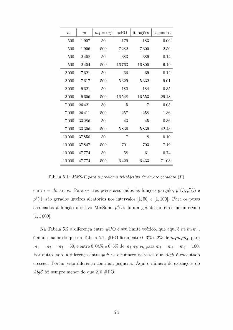
Grafos aleatorios nao-orientados com n nos, n = 500, 2 000, 7 000 e 10 000, foram

gerados para este problema tri-objetivo da arvore geradora. Para cada no, d nos

adjacentes sao gerados aleatoriamente, d = 8, 10. Uma verificacao e feita durante

a geracao destes arcos garantindo que o grau de cada no seja no maximo d. Desta

forma, pela nao-orientacao destes grafos temos que o numero de arcos m sera sempre

menor ou igual a dn/2, como pode ser visto na Tabela 5.1. Os tres pesos de cada

arco, p1(.), p2(.) e p3(.), tambem sao gerados aleatoriamente. Para p1(.) e p2(.), que

estao associados as funcoes gargalo, geramos inteiros nos intervalos [1, 50] e [1, 500].

Para os pesos associados a funcao objetivo MinSum, p3(.), foram gerados inteiros

no intervalo [1, 1 000].

Um importante comentario sobre a Tabela 5.1 se refere a cardinalidade do con-

junto mınimo completo (#PO). O limite teorico e dado por m1m2, que neste caso e

2 500 para mk = 50 e 250 000 para mk = 500, k = 1, 2. Porem, estes experimentos

mostram que #PO pode ser bem menor. Para mk = 50 temos que #PO esta entre

0, 2% e 15% de m1m2 e, para mk = 500, #PO esta entre 0, 1% e 6, 7% de m1m2.

Uma outra importante observacao diz respeito a diferenca entre #PO e o numero

de vezes que AlgS e executado (coluna iteracoes). Esta diferenca foi muito pequena,

o que e um resultado muito bom para o algoritmo MMS-B, pois como o mecanismo

destes algoritmos consiste em encontrar no maximo uma solucao por iteracao, entao

temos que #PO e um limite inferior para o numero de iteracoes.

Para o problema de caminho com quatro objetivos citado no inıcio desta secao,

foram gerados grafos aleatorios orientados com n nos, n = 1 000, 5 000, 8 000 e 15 000.

Para cada no, d sucessores sao escolhidos aleatoriamente, d = 5, 20, o que implica

23

n m m1 = m2 #PO iteracoes segundos

500 1 907 50 179 183 0.06

500 1 906 500 7 282 7 300 2.56

500 2 408 50 383 389 0.14

500 2 404 500 16 763 16 800 6.19

2 000 7 621 50 66 69 0.12

2 000 7 617 500 5 329 5 332 9.01

2 000 9 621 50 180 184 0.35

2 000 9 606 500 16 548 16 553 29.48

7 000 26 421 50 5 7 0.05

7 000 26 411 500 257 258 1.86

7 000 33 286 50 43 45 0.36

7 000 33 306 500 5 836 5 839 42.43

10 000 37 850 50 7 8 0.10

10 000 37 847 500 701 703 7.19

10 000 47 774 50 58 61 0.74

10 000 47 774 500 6 429 6 433 71.03

Tabela 5.1: MMS-B para o problema tri-objetivo da arvore geradora (P ).

em m = dn arcos. Para os tres pesos associados as funcoes gargalo, p1(.), p2(.) e

p3(.), sao gerados inteiros aleatorios nos intervalos [1, 50] e [1, 100]. Para os pesos

associados a funcao objetivo MinSum, p4(.), foram gerados inteiros no intervalo

[1, 1 000].

Na Tabela 5.2 a diferenca entre #PO e seu limite teorico, que aqui e m1m2m3,

e ainda maior do que na Tabela 5.1. #PO ficou entre 0.3% e 2% de m1m2m3, para

m1 = m2 = m3 = 50, e entre 0, 04% e 0, 5% de m1m2m3, para m1 = m2 = m3 = 100.

Por outro lado, a diferenca entre #PO e o numero de vezes que AlgS e executado

cresceu. Porem, esta diferenca continua pequena. Aqui o numero de execucoes do

AlgS foi sempre menor do que 2, 6 #PO.

24

n m m1 = m2 = m3 #PO iteracoes segundos

1 000 5 000 50 332 711 0.17

1 000 5 000 100 420 1 075 0.28

1 000 20 000 50 1 294 2 605 1.44

1 000 20 000 100 1 939 4 736 2.53

5 000 25 000 50 522 998 1.53

5 000 25 000 100 931 2 071 2.88

5 000 100 000 50 2 025 3 810 13.42

5 000 100 000 100 2 839 6 213 21.70

8 000 40 000 50 722 1 348 3.25

8 000 40 000 100 978 2 134 4.87

8 000 160 000 50 2 441 4 552 27.18

8 000 160 000 100 4 184 9 113 53.40

15 000 75 000 50 765 1 370 7.65

15 000 75 000 100 926 2 007 10.65

15 000 300 000 50 2 448 4 487 56.91

15 000 300 000 100 4 712 10 133 112.55

Tabela 5.2: MMS-B para o problema de caminho com quatro objetivos (P ).

25

Capıtulo 6

Consideracoes finais

Este trabalho resultou no desenvolvimento de algoritmos polinomiais para a

obtencao de um conjunto mınimo completo de solucoes Pareto-otimas para proble-

mas multi-objetivo em grafos. Varias implementacoes para o problema de caminho

tri-objetivo com duas funcoes objetivo MinMax e uma MinSum foram desenvolvi-

das e comparadas. Alem disso, tambem foram desenvolvidas implementacoes para

o problema de caminho com quatro objetivos e para os problemas tri-objetivo de

arvore geradora e de arvore de Steiner. Em todos estes problemas temos apenas

uma funcao objetivo totalizadora. Todas as demais funcoes objetivo consideradas

sao de gargalo.

Os problemas considerados nesta tese ainda nao haviam sido tratados na lite-

ratura de otimizacao combinatoria multi-objetivo. Por este motivo, aplicacoes foram

apresentadas para justificar o nosso interesse pelos problemas. Os trabalhos an-

teriores mais proximos sao os de Hansen [18], Martins [23] e Berman et al [4],

onde algoritmos bi-objetivo sao apresentados para o problema de caminho com uma

funcao MinSum e uma MinMax.

Os experimentos computacionais realizados mostraram que o algoritmo MMS-B

foi sempre mais eficiente do que os demais metodos, mesmo tendo a mesma com-

plexidade no pior caso. Isto se deve ao fato de que, teoricamente, o numero de vezes

que AlgS e executado no MMS-B e sempre menor ou igual comparado aos outros

26

metodos, e para os problemas gerados nos testes computacionais, a quantidade de

execucoes de AlgS pelo MMS-B foi sempre estritamente menor.

No problema de arvore de Steiner considerado neste trabalho, em uma das

funcoes objetivo de gargalo, ao inves de minimizar o maximo (ou maximizar o

mınimo) peso dos arcos, para algum peso pk(.), o interesse consiste em minimizar

o numero de nos intermediarios entre a raiz e o no mais distante. Isto se deve a

aplicacao que motivou o estudo deste problema tri-objetivo, apresentada no Capıtulo

2. Mesmo considerando este tipo de funcao gargalo foi possıvel desenvolver um al-

goritmo polinomial para o problema, o qual e similar ao algoritmo MMS-B. Por-

tanto, assim como foi possıvel tratar este problema tri-objetivo de arvore de Steiner

em tempo polinomial, possivelmente outros problemas de otimizacao combinatoria

multi-objetivo tambem podem ser resolvidos polinomialmente adaptando o algo-

ritmo MMS-B.

Antes de trabalhar na adaptacao do algoritmo MMS-B para outros problemas de

otimizacao combinatoria, julgamos que seja importante apresentar aplicacoes para

justificar o interesse pelos problemas. Da mesma forma que na aplicacao para o

problema tri-objetivo de arvore de Steiner surgiu uma funcao gargalo diferente, isto

e, definida sobre os nos e nao sobre os arcos, e possıvel que as funcoes objetivo

para esses outros problemas tambem tenham caracterısticas particulares. Logo, a

adaptacao do algoritmo vai depender das aplicacoes.

Restricoes adicionais podem ser consideradas pelos problemas que apresentamos

no Capıtulo 2. Mesmo incorporando restricoes de gargalo aos problemas (P ) e (P1),

ou seja:

max(i,j)∈s

{pk(i, j)} ≤ β ou min(i,j)∈s

{pk(i, j)} ≥ β,

onde β e um valor dado e pk(.) e um peso adicional (ou pode ser algum dos pesos

ja existentes), eles continuam podendo ser resolvidos polinomialmente pelos algo-

ritmos apresentados nesta tese. Para este tipo de restricoes basta eliminar, antes

da execucao dos algoritmos, os arcos (i, j) tais que pk(i, j) > β ou pk(i, j) < β,

respectivamente. Esta eliminacao de arcos implica na reducao de pesos distintos as-

sumidos pelas funcoes gargalo. Temos que essa quantidade de pesos distintos limita

27

o numero de iteracoes executadas pelos algoritmos. Logo, os algoritmos ficam mais

eficientes caso restricoes de gargalo sejam incorporadas aos problemas.

Caso restricoes do tipo totalizadoras sejam incorporadas ao problema (P ), como

por exemplo:∑

(i,j)∈s

pk(i, j) ≤ β ou∏

(i,j)∈s

pk(i, j) ≥ β,

com k 6= l + 1, entao (P ) se torna NP-difıcil, por exemplo, para o problema de

caminho (veja Hansen [18]) e para o problema da arvore geradora (veja Camerini et

al [5]).

O acrescimo de uma restricao totalizadora ao problema (P1), como a primeira

do paragrafo acima, leva a uma variante do Prize-Collecting Steiner Tree Problem

que e NP-difıcil (veja Costa et al [9]).

28

Referencias Bibliograficas

[1] Ahuja, R. K., Magnanti, T. L., Orlin, J. B. “Network Flows: Theory, Algorithms

and Applications”. Prentice Hall, New Jersey, 1993.

[2] Azevedo, J. A., Martins, E. Q. V. “An algorithm for the multiobjective shortest

path problem on acyclic networks”. Investigacao Operacional, v. 11 (1),

pp. 52–69, 1991.

[3] Bellman, R. E. “On a routing problem”. Quart. Appl. Math., v. 16, pp. 87–90,

1958.

[4] Berman, O., Einav, D., Handler, G. “The constrained bottleneck problem in

network”. Operations Research, v. 38, pp. 178–181, 1990.

[5] Camerini, P. M., Galbiati, G., Maffioli, F. “The complexity of multi-constrained

spanning tree problems”. In: Theory of Algorithms, L. Lovasz (ed.), Col-

loquium, Pecs 1984. North-Holland, Amsterdam 53–101, 1984.

[6] Canuto, S. A., Resende, M. G. C., Ribeiro, C. C. “Local search with perturba-

tions for the prize-collecting Steiner tree problem in graphs”. Networks,

v. 38, pp. 50–58, 2001.

[7] Clımaco, J. C. N., Martins, E. Q. V. “A bicriterion shortest path algorithm”.

European Journal of Operational Research, v. 11, pp. 399–404, 1982.

[8] Costa, A. M., Cordeau, J. -F., Laporte, G. “Steiner tree problems with profits”.

INFOR, v. 44, pp. 99–115, 2006.

29

[9] Costa, A. M., Cordeau, J. -F., Laporte, G. “Models and branch-and-cut al-

gorithms for the Steiner tree problem with revenues, budget and hop

constraints”. Networks, v. 53, pp. 141–159, 2008.

[10] Cunha, A. S., Lucena, A., Maculan, N., Resende, M. G. C. “A relax-and-cut

algorithm for the prize-collecting Steiner problem in graphs”. Discrete

Applied Mathematics, v. 157, pp. 1198–1217, 2009.

[11] Dijkstra, E. W. “A note on two problems in connexion with graphs”. Numer.

Math., v. 1, pp. 269–271, 1959.

[12] Ehrgott M., Gandibleux, X. “A survey and annotated bibliography of multi-

objective combinatorial optimization”. OR Spektrum, v. 22, pp. 425–460,

2000.

[13] Gabow, H. N., Galil, Z., Spencer, T., Tarjan, R. E. “Efficient algorithms for

finding minimum spanning trees in undirected and directed graphs”. Com-

binatorica, v. 6, pp. 109–122, 1986.

[14] Gabow, H. N., Tarjan, R. E. “Algorithms for two bottleneck optimization prob-

lems”. Journal of Algorithms, v. 9, pp. 411–417, 1988.

[15] Gandibleux, X., Beugnies, F., Randriamasy, S. “Martins’ algorithm revisited

for multi-objective shortest path problems with a MaxMin cost function”.

A Quarterly Journal of Operations Research, v. 4, pp. 47–59, 2006.

[16] Gouveia, L. “Multicommodity flow models for spanning trees with hop con-

straints”. European Journal of Operational Research, v. 95, pp. 178–190,

1996.

[17] Guerriero, F., Musmanno R. “Label correcting methods to solve multicriteria

shortest path problems”. Journal of Optimization Theory and Applica-

tions, v. 111, n. 3, pp. 589–613, 2001.

30

[18] Hansen, P. “Bicriterion path problems”. In: Multicriteria decision making: the-

ory and applications, Lecture Notes in Economics and Mathematical Sys-

tems, 177, G. Fandel and T. Gal (eds.), Springer, Heidelberg, 109–127,

1980.

[19] Johnson, D. S., Minkoff, M., Phillips, S. “The prize collecting Steiner tree

problem: theory and practice”. Proceedings of the 11th ACM-SIAM Sym-

posium on Discrete Algorithms, San Francisco, 2000.

[20] Kruskal, J. B. “On the Shortest Spanning Subtree of a graph and the Travelling

Salesman Problem”. Proc. Amer. Math. Soc., v. 7, pp. 48–50, 1956.

[21] Koopmans, T. C. “Analysis of production as an efficient combination of activ-

ities”. In: Activity Analysis of Production and Allocation (Chap. III), ed.

T. C. Koopmans, John Wiley & Sons, New York, pp. 33–97, 1951.

[22] Martins, E. Q. V. “On a multicriteria shortest path problem”. European Journal

of Operational Research, v. 16, pp. 236–245, 1984.

[23] Martins, E. Q. V. “On a special class of bicriterion path problems”. European

Journal of Operational Research, v. 17, pp. 85-94, 1984.

[24] Pareto, V. “Course d’Economic Politique”. Lausanne, Rouge, 1896.

[25] Pinto, L. L. “Um algoritmo polinomial para problemas tri-objetivo de

otimizacao de caminhos em grafos”. 2007. 34 p. Dissertacao (Mestrado

em Engenharia de Sistemas e Computacao) - Programa de Engenharia de

Sistemas e Computacao, COPPE, UFRJ, Rio de Janeiro–RJ, 2007.

[26] Pinto, L. L., Bornstein, C. T. “Software CamOtim”. Disponıvel em:

http://www.cos.ufrj.br/camotim, 2006.

[27] Pinto, L. L., Bornstein, C. T. “Efficient solutions for the multi-objective optimal

path problem in graphs”. Anais do Premiere Conference Internationale

en Calcul de Variations et Recherche Operationelle, Ouidah–Benin, 2007.

31

[28] Pinto, L. L., Bornstein, C. T., Maculan N. “The tricriterion shortest path prob-

lem with at least two bottleneck objective functions”. European Journal

of Operational Research, v. 198, pp. 387–391, 2009.

[29] Pinto, L. L., Bornstein, C. T., Maculan N. “Um problema de caminho

tri-objetivo”. Anais do XL SBPO, Joao Pessoa–PB, pp. 1032–1042,

2008.(http://www.cos.ufrj.br/∼leizer/MMS-R.pdf)

[30] Pinto, L. L., Bornstein, C. T., Maculan N. “A reverse algorithm for the tricri-

terion shortest path problem”. Anais do XXXIX Annual Conference of

Italian Operational Research Society, Ischia–Italy, 2008.

[31] Pinto, L. L., Bornstein, C. T., Maculan N. “A polynomial algorithm for the

multi-objective bottleneck network problem with one MinSum objective

function”. Submetido para Networks, 2008.

[32] Pinto, L. L., Laporte, G. “An effcient algorithm for the Steiner tree problem

with revenue, bottleneck and hop objective functions”. Submetido para

European Journal of Operational Research, 2009.

[33] Pinto, L. L., Pascoal, M. “Enhanced algorithms for tricriteria

shortest path problems with two bottleneck objective func-

tions”. Relatorios de Investigacao, n. 3, INESC–Coimbra, 2009.

(http://www.inescc.pt/documentos/3 2009.pdf)

[34] Pinto, L. L., Pascoal, M. “On algorithms for the tricriteria shortest path prob-

lem with two bottleneck objective functions”. Submetido para Computers

& Operations Research, 2009.

[35] Prim, R. C. “Shortest connection networks and some generalisations”. Bell

System Technical Journal, v. 36, pp. 1389–1401, 1957.

[36] Serafini, P. “Some considerations about computational complexity for multi

objective combinatorial problems”. In: Recent advances and historical de-

32

velopment of vector optimization. Lecture Notes in Economics and Math-

ematical Systems, 294, W. Krabs and J. Jahn (eds.), Springer, Berlin,

Heidelberg, New York, 222–232, 1987.

[37] Tung, C. T., Chew, K. L. “A bicriterion Pareto–optimal path algorithm”. Asia–

Pacific Journal of Operational Research, v. 5, pp. 166–172, 1988.

[38] Tung, C. T., Chew, K. L. “A multicriteria Pareto–optimal path algorithm”.

European Journal of Operational Research, v. 62, pp. 203–209, 1992.

[39] Zeleny, M. “Linear Multiobjective Programming”. Lecture Notes in Economics

and Mathematical Systems, 95, Springer-Verlag, 1974.

[40] Zelikovsky, A. “Bottleneck Steiner Tree Problems”. In: Encyclopedia of Opti-

mization, 2nd edition, C. A. Floudas and P. M. Pardalos (Eds.), Springer,

New York, 311–313, 2009.

33

Anexo 1

Este anexo contem o artigo:

Pinto, L. L., Bornstein, C. T., Maculan N. “The tricriterion shortest path problem

with at least two bottleneck objective functions”. European Journal of Operational

Research, v. 198, pp. 387–391, 2009.

34

1

The tricriterion shortest path problem with at least two bottleneck objective functions

Leizer de Lima Pinto

Cláudio Thomás Bornstein

Nelson Maculan

COPPE/UFRJ – Federal University of Rio de Janeiro, Brazil

Dept. of Systems Engineering and Computer Science

Abstract: The focus of this paper is on the tricriterion shortest path problem where two objective

functions are of the bottleneck type, for example MinMax or MaxMin. The third objective function

may be of the same kind or we may consider, for example, MinSum or MaxProd. Let ( )np be the

complexity of a classical single objective algorithm responsible for this third function where n is the

number of nodes and m be the number of arcs of the graph. An ( )( )npmO 2 algorithm is presented

that can generate the minimal complete set of Pareto-optimal solutions. Finding the maximal

complete set is also possible. Optimality proofs are given and extensions for several special cases

are presented. Computational experience for a set of randomly generated problems is reported.

Keywords: Multicriteria shortest path problem, Pareto-optimal solution.

1) Introduction:

Traditionally the shortest path (SP) problem considers just one objective function which

generally consists in minimizing the sum (MinSum) of the weights of the path. This problem may

be solved for non-negative weights by a label-setting (LS) algorithm, Dijkstra for example, or in the

general case by a label-correcting (LC) algorithm. For more details see Ahuja et al. (1993).

Gondran & Minoux (1986) generalize these results considering several other functions like

MaxSum, MaxProd and MaxMin. An extension for the MinMin and MaxMax problem is also

possible but few applications for these cases have been reported. Additionally, the results may be

extended for the MinProd and MinMax cases. A free software for the optimization of the problems

mentioned above is available at Pinto & Bornstein (2006a) and is reported in Pinto & Bornstein

(2006b).

Many SP-problems consider more than one objective function. Applications for the multi-

objective SP-problem are given in Batta & Chiu (1988), Current & Min (1986) and Current &

Marsh (1993). For the multi-objective problem, also called the vector optimization problem, it

seems more reasonable to determine the set of nondominated (Pareto-optimal) solutions instead of

finding an optimal solution. For each nondominated vector we may be interested in giving just one

or giving the set of all corresponding solutions, leading to the generation of the minimal or the

maximal complete set of Pareto-optimal solutions respectively.

Initial definitions of nondominance were given by Pareto (1896). These concepts were used

in OR for the first time by Koopmans (1951). An introduction in multi-objective linear

programming is given by Zeleny (1974).

Martins (1984a) presents a non-polynomial LS-algorithm for the MinSum multi-objective

SP-problem. For the same problem Guerriero & Musmanno (2001) give a non-polynomial LC-

algorithm. An extension of Martins’ algorithm is presented in Gandibleux et al. (2006) where in

addition to MinSum, one MaxMin objective is also considered. Multi-objective SP-problems are

also examined in Azevedo & Martins (1991), Clímaco & Martins (1981), Corley & Moon (1985),

Tung & Chew (1992), Sastry et al (2003) and Sastry et al (2005).

Hansen (1980) proves that for the MinSum-MinSum bicriterion SP-problem, the cardinality

of the minimal complete set increases exponentially with the size of the graph. As a matter of fact,

multi-objective SP-problems with more than one MinSum objective are NP-hard (see Gandibleux et

2

al (2006)). This result can be extended for other functions. Clímaco & Martins (1982), Current et al

(1987) and Tung & Chew (1988) also work with the SP-problem with two MinSum objectives.

Hansen (1980) presents an ( )nlogmO 2 algorithm for the bicriterion SP-problem with at

least one MinMax/MaxMin bottleneck objective function. The other objective function may either

be MinMax/MaxMin or MinSum/MaxSum. Berman et al (1990) develop an ( )( )npmO algorithm

for the MinMax-MinSum bicriterion SP-problem. Consequently, Hansen’s algorithm is less

efficient for dense graphs. For the same kind of problem Martins (1984b) presents an algorithm

with the same complexity as Hansen’s.

Here the focus is on the tricriterion SP-problem with at least two bottleneck objective

functions. In section 2 an example of an application for the MaxMin-MinMax-MinSum problem is

given, followed by the formulation of an ( )( )npmO 2 algorithm that is able to produce the minimal

complete set of Pareto-optimal solutions. Three different weights ( )j,ip1 , ( )j,ip2 and ( )j,ip3

for each arc ( )j,i , corresponding to each of the three objectives, may be considered. The algorithm

orders the weights of the arcs, generating subgraphs with arcs introduced successively so as to

satisfy lower/upper bounds for ( )j,ip1 and ( )j,ip2 . For each such subgraph the algorithm

searches for a MinSum solution. A new Pareto-optimum is obtained if this solution means an

improvement with respect to a set of solutions generated previously. The procedure has some

similarities with the algorithm presented by Berman et al (1990) but the fact that we consider two

bottleneck objectives instead of just one makes it necessary to introduce an additional test. An

extension of the algorithm allows the generation of the set of all Pareto-optimal solutions (maximal

complete set). Optimality proofs are given.

Section 3 presents computational results for a set of randomly generated problems up to

5000 nodes and section 4 extends some of the previous results closing the paper with the

conclusions.

2) The MaxMin-MinMax-MinSum problem:

Let ( )M,N G = be a graph with n|N| = and m|M| = . Real functions ( )j,ip1 ,

( )j,ip2 and ( )j,ip3 are associated with each arc ( ) Mji, ∈ . Let 1m and 2m be the quantity of

different values assumed by 1p and 2p respectively. Without loss of generality let us suppose that

the 1m values 1m

12

11 1

p,,p,p K and the 2m values 2m

22

21 2

p,,p,p K are arranged in an

decreasing/increasing order respectively, i.e., we have 1m

12

11 1

ppp >>> L and

2m

22

21 2

ppp <<< L .

Let ( ) ( ) ( ){ }2g

21r

1rg pi, j pand pi, jp|Mi, jM ≤≥∈= and let ( )

rgrg MN,G = be a

spanning subgraph of G. Of course we have g'r'rg MM ⊇ for rr' ≤ and gg' ≤ . It is also easy to

see that MM21mm = .

A path in G from Ns ∈ to Nt ∈ is the ordered set { }t ,i ,. . . ,i ,i s, P h21st = where

Ni ,. . . ,i ,i h21 ∈ . { }1h21st a,,a,aAP += K , with ( ) ( ) ( ) Mt,ia,...,,iia,i,sa h1h21211 ∈=== + is the

set of arcs belonging to the path. Let stGS be the set of all paths from s to t in G. In this section we

are interested in the following tricriterion shortest path problem:

3

( ){ }

( ){ }

( )

.SP :to ubject s

ji,p minimize

ji,pmax minimize

ji,pmin maximize(P)

stGst

APj)(i,

3

2

APj)(i,

1

APj)(i,

st

st

st

∈

∑∈

∈

∈

For example, in a road transportation problem ( )ji,p1 may represent the quality of the

road between points i and j. 1m labels are available to evaluate this quality and the smaller the label

the worse the road. ( )ji,p2 measures traffic density and finally ( )ji,p3 represents the cost or time

of the trip which can be proportional to the distance between i and j. A transportation company may

be interested in simultaneously minimizing costs, traffic jam delays and maximizing the quality of

the roads used by their vehicles. We could imagine that there were no ways of reducing all three

objectives to a common measure (costs for example). At a first stage the management may be

interested in generating all nondominated solutions. At a later stage, those responsible for the route

planning may need appropriate criteria for making the final choice either automatically or manually,

by inspection. The first option is more attractive in the case of a great number of solutions. It is

possible to decrease them by introducing, additionally, upper or lower bounds for some of the

objectives. We will be examining this situation in section 4.

The definitions of Pareto-optimum, minimal and maximal complete set follow. Let problem

(P) be considered for graph G. Let ( ) 3P

3

P

2

P

1

P q ,q ,qq stststst ℜ∈= be the objective vector associated

with path stP where ( ){ }ji,pminq 1

APj)(i,

P

1st

st

∈= , ( ){ }ji,pmaxq 2

APj)(i,

P

2st

st

∈= and ( )∑

∈

=st

st

APj)(i,

3P

3 ji,pq . A path

stP dominates another path stP if stst P

1

P

1 qq ≥ , stst P

2

P

2 qq ≤ and stst P

3

P

3 qq ≤ with at least one of the

inequalities being satisfied strictly. Following definitions can be made:

(a) stP is a Pareto-optimum path if there is no other path stP ∈ stGS that dominates stP .

(b) A set *C of different Pareto-optimal solutions is said to be a minimal complete set if for

any Pareto-optimal solution stP one of the two conditions below apply:

(b1) *st CP ∈ and there is no *

st CP ∈ , stst PP ≠ so that stst PP qq = .

(b2) *st CP ∉ and there is one and only one *

st CP ∈ so that stst PP qq = .

(c) The set of all Pareto-optimal solutions is called the maximal complete set.

It is easy to show that 4221

* nmm m||C ≤≤≤ , i.e., the cardinality of the minimal complete

set *C is polinomially bounded by 4n . From the definition (b) of minimal complete set it should be

clear that for each *st CP ∈ a different value of the objective vector ( )stst P

3

2

g

1

r

Pq ,p ,p q = is

associated, meaning that there can be no more elements in *C than the number of different values

of stPq . With respect to the first two elements of stPq there can be no more than 21mm different

values. But for each pair of values 1rp , 2

gp , one and only one value stP

3q is possible.

The next step consists in presenting algorithm Min-Max-Sum (MMS) which solves problem

(P) determining a minimal complete set *C . Of course there may be more than one set of this kind.

The algorithm consists of two loops. The outer i-loop corresponds to decreasing values of 1p and

the inner j-loop corresponds to increasing values of 2p . For each pair of values i, j a graph ijG is

4

generated in order to search for an optimal path stP with respect to the MinSum criterion. This is

done with the help of AlgS at step 3.1.1 and a classical LS or LC-algorithm can be used to obtain the

value of stP

3q . In order to have a Pareto-optimum, stP

3q has to represent an improvement. This is

checked at step 3.1.3 using variable kv . 1Q , 2Q and 3Q are sets containing the values of the three

objective functions corresponding to the Pareto-optimal solutions included in *C .

1. Given: ( )M,N G = , s, t

2. Do: ∅=:C* , ∅=:Q1 , ∅=:Q2 , ∅=:Q3 and 2k m,2, 1, k for:v K=∞=

3. For i from 1 to 1m do

3.1. For j from 1 to 2m do

3.1.1. Use AlgS to determine the optimal path in ijG

3.1.2. Let stP be the optimal path. If there is no path from s to t, set ∞=stP

3q

3.1.3. If { }

<

≤≤k

jk1

P

3 v minq st then

3.1.3.1. stP

3j q:v =

3.1.3.2. { }st** PC:C U=

3.1.3.3. { }1i11 pQ:Q U= , { }2

j22 pQ:Q U= and { }stP

333 qQ:Q U=

3.2. End

4. End

It is easy to show that the complexity of algorithm MMS is ( )( )npmO 2 . Two loops of size

1m and 2m , with mm,m 21 ≤ lead to 2m iterations in the worst case. Each iteration uses AlgS of

complexity ( )np . For example, if the graph has non-negative weights an 2n -Dijkstra algorithm

may be used for AlgS, i.e. ( ) 2nnp = , and the result is an ( )22nmO algorithm for MMS. We are

supposing that ( ) 2nnp ≥ (step 3.1.3 is ( )2nO ).

Next it will be proved that *C is a minimal complete set. Theorem 1 proves that all stP

generated by algorithm MMS are Pareto-optimal solutions. Theorem 2 uses theorem 1 to prove that *C is a minimal complete set. Let iteration ri = and gj = be called the rg-iteration.

Theorem 1: Let stP be the path inserted in *C at the rg-iteration of algorithm MMS. Following

two facts are true:

(a) 1r

P

1 pq st = and 2g

P

2 pq st = ;

(b) stP is a Pareto-optimal solution of (P).

Proof:

(a) It will be shown by contradiction that the values 1rp and 2

gp associated to stP by algorithm

MMS are effectively the values stP

1q and stP

2q of the two bottleneck functions MaxMin and

MinMax. Since stP was obtained for rgG we have ( ) 1r

1 p hl,p ≥ and ( ) 2g

2 p hl,p ≤ for all

( ) stPAhl, ∈ . It follows that 1r

P

1 pq st ≥ and 2g

P

2 pq st ≤ . Suppose that 1r

1r'

P

1 ppq st >= and

5

2g

2g'

P

2 ppq st ≤= (the other case can be proven in a similar way). Consequently, all arcs

( ) stPAhl, ∈ have ( ) 1r'

1 p hl,p ≥ and ( ) 2g'

2 p hl,p ≤ . By definition, it follows that r'r < and

g'g ≤ . Hence stP is a path in graph 'g'rG at the r’g’-iteration preceding the rg-iteration.

This leads to a contradiction because step 3.1.3 guarantees that if stP is a path at the r’g’-

iteration it could never have been included in *C at the rg-iteration. Thus, it can be stated

that 1r

P

1 pq st = . A similar reasoning proves 2g

P

2 pq st = .

(b) Again the proof is by contradiction. Suppose that stP is not a Pareto-optimal solution. Then,

by definition, there exists a path stP that dominates stP . Using (a) it can be said that

1r

P

1

P

1 pqq stst =≥ , 2g

P

2

P

2 pqq stst =≤ and stst P

3

P

3 qq ≤ with at least one of the inequalities being

satisfied strictly. Without loss of generality consider the case where 1r

P

11r'

P

1 pqpq stst =>=

and 2g

P

22g'

P

2 pqpq stst =≤= . The proof of the other cases is similar. From the initial

assumptions of this section it follows that rr' < , gg' ≤ and stP is a path in graph 'g'rG at

the r’g’-iteration preceding the rg-iteration. Due to step 3.1.3 at the end of the r’g’-iteration,

there must exist a path *st CP ∈ better or equal than stP . stP may have been generated at the

r’g’-iteration or may have been generated at a previous iteration. Of course it is possible that

stP = stP . Using the inequality from the beginning of the paragraph it can be stated that

ststst P

3

P

3

P

3 qqq ≤≤ . On the other side, step 3.1.3 used at the rg-iteration guarantees that

{ } { } stst P

3kg'k1

kgk1

P

3 qv min v minq ≤≤<≤≤≤≤

leading to a contradiction.

▀

Theorem 2: Algorithm MMS produces, upon completion, a minimal complete set *C of Pareto-

optimal solutions of problem (P).

Proof: Part (b) of theorem 1 shows that *C is a set of Pareto-optimal solutions. Part (a) shows that

any two solutions stP and stP included in *C by algorithm MMS are different with stst PP qq ≠ .

Thus, part (b1) of the definition of minimal complete set is satisfied.

Next, part (b2) of the definition will be examined. Let *st CP ∉ be a Pareto-optimal

solution so that 1r

P

1 pq st = and 2g

P

2 pq st = . stP is a path in graph rgG . Therefore there exists a path

stP obtained at step 3.1.2 of the rg-iteration. The fact that stP was obtained in graph rgG ,

guarantees that ( ) 1r

1 p hl,p ≥ and ( ) 2g

2 p hl,p ≤ for all ( )stPAhl, ∈ . This results in stst P

11r

P

1 qpq =≥

and stst P

22g

P

2 qpq =≤ . Furthermore, optimality of AlgS guarantees that stst P

3

P

3 qq ≤ . The fact that stP

is a Pareto-optimal solution assures that none of these inequalities can be satisfied strictly, leading

to stst PP qq = . Thus, stP is also a Pareto-optimal solution.

It is easy to show that at step 3.1.3 of the rg-iteration the condition { }kgk1

P

3 v minq st

≤≤< is

satisfied, leading to *st CP ∈ . If { }k

gk1

P

3 v minq st

≤≤≥ there would exist a path *

st CP ∈ , inserted at a

6

previous r’g’-iteration, so that stst P

3

P

3 qq ≤ . Evidently rr' ≤ and gg' ≤ , with at least one of the

inequalities being satisfied strictly. Thus, stP would be dominated by stP , since (a) of theorem 1

guarantees that stst P

11r

1r'

P

1 qppq =≥= and stst P

22g

2g'

P

2 qppq =≤= , with at least one of the

inequalities being satisfied strictly. Consequently stP would not be a Pareto-optimal solution

leading to a contradiction. Hence stP satisfies test 3.1.3 and is inserted in *C satisfying (b2).

▀

To generate the maximal complete set it is just necessary to replace AlgS by an algorithm

which generates the set of all optimal solutions at step 3.1.1 and then make the necessary

adjustments. One should remember that the cardinality of this set increases exponentially with the

size of the problem (in the worst case all paths are optimal). Thus, an algorithm to generate the

maximal complete set is necessarily non-polynomial (NP) (see also Ehrgott and Gandibleux

(2000)).

3) Computational results:

This section presents computational results for a set of randomly generated problems. Each

line of table 1 represents the average values of three problems. Nine classes of problems Probij for i,

j = 1, 2 and 3 are generated. i = 1, 2 and 3 represents a graph with 50, 1000 and 5000 nodes

respectively. j = 1, 2 and 3 represents increasing graph densities. For each pair of nodes Nh,l ∈

an integer k is generated randomly between 1 and α . If k=1 then ( ) Mh,l ∈ . Otherwise, there will

be no corresponding arc associated to the graph. j = 1, 2 and 3 corresponds to 2,10=α and 1

respectively. Of course for 1=α the graph is complete. For each class, three kinds of problems are

produced with respect to values for 1p and 2p , generating integers randomly for the interval [1,

5], [1, 20] and [1, 70] respectively. With respect to 3p , integers are generated randomly between 1

and 10000 for each of the three cases.

Problems were run on a PC with a CENTRINO CORE DUO processor at 1.6 GHz with

1024 Mb of RAM. Programming language was C and a heap implementation of Dijkstra’s algorithm

was used for AlgS.

At table 1 cms and cMs are the average cardinality of the minimal and maximal complete

set respectively. timecms and timecMs are the average computer times in seconds that were necessary

to generate the corresponding sets.

A first comment relates to the values obtained for cms and cMs as well as the corresponding

timecms and timecMs. Very similar values were obtained. This may be due to the special data which

was used, particularly the values of 3p which were generated from a rather large interval,

producing few paths with the same length. An experience was made, generating 3p from a [1, 10]

interval and the results were quite different. Again, nine problems were considered for each class.

Instead of having cMs/cms = 1.0 as in table 1 the results for the new set of problems were

1.0 ≤≤ cmscMs 5.9. For example, the average values for the class Prob23 with m1 = m2 = 5

were cms = 6 and cMs = 16.

Another more important conclusion refers to the small increase of cms or cMs with respect

to increasing values of m and n. Comparing the problems obtained for n = 1000 with the problems

obtained for n = 5000 we see that almost the same number of Pareto-optimal solutions was

obtained. Even if we compare n = 50 with n = 1000, representing an increase of the size of the

graph of approximately 20 times, the corresponding increase of the average cms of nearly 6 times is

far below. These conclusions are reinforced comparing increasing values of m for a certain fixed

7

Class n m m1 = m2 cms timecms cMs timecMs

Prob11 50 259 5 6 0 6 0

Prob11 50 237 20 8 0 8 0

Prob11 50 254 69 4 0 4 0

Prob12 50 1230 5 12 0 12 0

Prob12 50 1219 20 32 0 32 0

Prob12 50 1222 70 40 0 40 0

Prob13 50 2450 5 15 0 15 0

Prob13 50 2450 20 34 0 34 0

Prob13 50 2450 70 60 0 60 0

Prob21 1000 99942 5 21 0 21 0

Prob21 1000 99885 20 103 2 103 2

Prob21 1000 99826 70 281 32 281 32

Prob22 1000 499567 5 17 0 17 0

Prob22 1000 499544 20 81 3 81 3

Prob22 1000 499558 70 304 53 304 54

Prob23 1000 999000 5 19 0 19 0

Prob23 1000 999000 20 113 5 114 5

Prob23 1000 999000 70 322 191 323 208

Prob31 5000 2499672 5 21 5 21 5

Prob31 5000 2500231 20 135 62 135 62

Prob31 5000 2500726 70 394 892 394 901

Prob32 5000 12497615 5 20 6 21 7

Prob32 5000 12497449 20 152 115 154 119

Prob32 5000 12497604 70 433 1246 435 1282

Prob33 5000 24995000 5 20 7 21 7

Prob33 5000 24995000 20 124 97 126 103

Prob33 5000 24995000 70 455 1529 458 1616

Table 1: Average values of times and the number of Pareto-optimal solutions.

value of n. With exception of the very small problems ( 50n = and 250m ≈ ) where the sparsity of

the graph led to a very small number of Pareto-optimal solutions, for a certain fixed value of n,

there is almost no change of cms with increasing values of m.

A greater sensitivity is verified when comparing the variation of cms or cMs with respect to

1m or 2m . With exception of the very small problems, one is tempted to establish an almost linear

relationship between cms or cMs and 1m or 2m . Anyway, the values obtained for cms or cMs seem

quite far from the upper limit 1m 2m . This is specially true for bigger values of 1m or 2m .

A general conclusion concerning the variation of cms or cMs is that the number of Pareto-

optimal solutions seems to increase rather slowly with n, m, 1m or 2m . At this stage it is quite hard

to tell if this result can be generalized or if it relates strongly to the kind of data which was used.

4) Extensions and conclusions:

The tricriterion SP-problem with at least two bottleneck objective functions, gives rise to a

series of different problems. If order does not matter, three problems arise with respect to the two

bottleneck functions MaxMin and MinMax: MaxMin-MinMax, MaxMin-MaxMin, MinMax-

MinMax. Now consider the six possibilities for the third objective function: MaxMin, MinMax,

MaxSum, MinSum, MaxProd and MinProd. The result is a set of eighteen similar problems which

can be solved by the algorithm MMS with some minor adjustments.

8

A different problem arises if we introduce additional restrictions into problem (P). An easy

case happens when these restrictions are of the bottleneck type, i.e., we require the maximum or

minimum weight of a path to be respectively lesser than or greater than a certain value. In this case

it is sufficient to delete the corresponding arcs from the graph (see Berman et al. (1990)).

Considering an upper bound for the sum of the weights 3p of the path is also easy to solve if we

work with the MinSum objective. If the solution obtained by AlgS for a certain value of i and j does

not satisfy the upper bound it will not be included in the minimum complete set. A similar comment

can be made if we consider a lower bound for a MaxSum objective. A more difficult problem

results from taking another weight, different from 3p , to evaluate these bounds.

A particular case for algorithm MMS occurs when 21 pp = where 321 ppp == is just a

special situation. Problems represented by a graph with just one weight per arc, where paths need to

be evaluated from several different perspectives, may fall under this case. The efficiency of

algorithm MMS is improved and approximately half of the number of iterations is needed to

generate the minimal complete set.

An extension for the tricriterion spanning tree problem is also possible. For the MaxMin-

MinMax-MinSum case it is sufficient to change at step 3.1.1 of algorithm MMS the AlgS by a

traditional minimum spanning tree algorithm like Prim or Kruskal. If instead of MinSum we have

another MinMax objective function it is sufficient to consider algorithms like those presented in

Camerini (1978) or Gabow & Tarjan (1988).

A last word should be said with respect to practical aspects of problem (P) and algorithm

MMS. As already seen, algorithm MMS needs 21mm iterations to generate *C . Hence, for big

values of 1m and 2m , there may be a lot of computational work involved. For a PC, as in our case,

it seems reasonable to have 100m,m 21 ≤ . As a matter of fact, for great values of 1m and 2m , the

determination of *C seems not to make much sense. A great number of Pareto-optima may leave

the decision maker in a difficult situation having to choose among a rather large set of possible

solutions. In contrast, for small values of 1m and 2m the number of Pareto-optima seems to

increase very slowly with the size of the graph meaning that big graphs can be treated quite

effectively.

References:

Ahuja RK, Magnanti TL, Orlin JB. Network flows. New Jersey; 1993.

Azevedo JA, Martins EQV. An algorithm for the multiobjective shortest path problem on acyclic

networks. Investigação Operacional 1991; 11 (1); 52-69.

Batta R, Chiu SS. Optimal obnoxious paths on a network: Transportation of hazardous materials.

Operations Research 1988; 36; 84-92.

Bellman RE. On a routing problem. Quarterly of Applied Mathematics 1958; 16; 87-90.

Berman O, Einav D, Handler G. The constrained bottleneck problem in networks. Operations

Research 1990; 38; 178-181.

Camerini PM. The min-max spanning tree problem and some extensions. Information Processing

Letters 1978; 7; 10-14.

Clímaco JCN, Martins EQV. On the determination of the nondominated paths in a multiobjective

network problem. Methods in Operations Research 1981; 40; 255-258.

Clímaco JCN, Martins EQV. A bicriterion shortest path algorithm. European Journal of Operational

Research 1982; 11; 399-404.

Corley HW, Moon ID. Shortest paths in networks with vector weights. Journal of Optimization

Theory and Applications 1985; 46; 79-86.

Current JR, Min H. Multiobjective design of transportation networks: Taxonomy and annotation.

European Journal of Operational Research 1986; 26; 187-201.

9

Current JR, Revelle CS, Cohon JL. The median shortest path problem: A multiobjective approach

to analyze cost vs. accessibility in the design of transportation networks. Transportation

Science 1987; 21 (3); 188-197.

Current JR, Marsh M. Multiobjective transportation network design and routing problems:

Taxonomy and annotation. European Journal of Operational Research 1993; 103; 426-438.

Dijkstra EW. A note on two problems in connexion with graphs. Numer. Math. 1959; 1; 269-271.

Ehrgott M, Gandibleux X. A survey and annotated bibliography of multiobjective combinatorial

optimization. OR Spektrum 2000; 22; 425-460.

Gabow HN, Tarjan RE. Algorithms for two bottleneck optimization problems. Journal of

Algorithms 1988; 9; 411-417.

Gandibleux X, Beugnies F, Randriamasy S. Martins’ algorithm revisited for multi-objective shortest

path problems with a MaxMin cost function. A Quarterly Journal of Operations Research

2006; 4; 47-59.

Guerriero F, Musmanno R. Label correcting methods to solve multicriteria shortest path problems.

Journal of Optimization Theory and Applications 2001; 111 (3); 589-613.

Gondran M, Minoux M. Graphs and Algorithms. John Wiley; 1986.

Hansen P. Bicriterion path problems. In: Fandel G, Gal T (Eds), Multicriteria decision making:

Theory and applications. Lecture Notes in Economics and Mathematical Systems, vol. 177.

Springer, Heidelberg; 1980. p. 109-127.

Koopmans TC. Activity analysis of production and allocation. John Wiley & Sons, New York;

1951.

Martins EQV. On a multicriteria shortest path problem. European Journal of Operational Research

1984a; 16; 236-245.

Martins EQV. On a special class of bicriterion path problems. European Journal of Operational

Research 1984b; 17; 85-94.

Pareto V. Course d’economic politique. Lausanne, Rouge; 1896.

Pinto LL, Bornstein CT. Software CamOtim. Available at: http://www.cos.ufrj.br/camotim; 2006a.

Pinto LL, Bornstein CT. Algoritmos para problemas de caminho ótimo em grafos (Algorithms for

optimal path problems in graphs). Proceedings of the XXXVIII Brazilian Symposium on

Operations Research. Goiânia-GO; 2006b; 2418-2419.

Sastry VN, Janakiraman TN, Mohideen SI. New algorithms for multi objective shortest path

problem. Opsearch 2003; 40; 278-298.

Sastry VN, Janakiraman TN, Mohideen SI. New polynomial time algorithms to compute a set of

Pareto optimal paths for multi-objective shortest path problems. International Journal of

Computer Mathematics 2005; 82; 289-300.

Tung CT, Chew KL. A bicriterion Pareto-optimal path algorithm. Asia-Pacific Journal of

Operational Research 1988; 5; 166-172.

Tung CT, Chew KL. A multicriteria Pareto-optimal path algorithm. European Journal of

Operational Research 1992; 62; 203-209.

Zeleny M. Linear Multiobjective Programming. Lecture Notes in Economics and Mathematical

Systems, vol. 95. Springer-Verlag; 1974.

Anexo 2

Este anexo contem o artigo de Pinto e Pascoal intitulado On algorithms for the

tricriteria shortest path problem with two bottleneck objective functions e submetido

a Computers & Operations Research. A versao inicial foi submetida em marco de

2009. Em maio recebemos as sugestoes dos revisores e as implementamos na atual

versao. Este anexo contem essa nova versao, submetida em setembro de 2009.

44

On algorithms for the tricriteria shortest path problem with two bottleneckobjective functions

Leizer Lima Pinto1,2 and Marta M. B. Pascoal∗3,4

1COPPE/UFRJ - Federal University of Rio de Janeiro, BrazilDepartment of Systems Engineering and Computer Science

E-mail: leizer@cos.ufrj.br

2Interuniversity Research Centre on Enterprise Networks, Logistics and Transportation (CIRRELT)

3Departamento de Matematica da Universidade de CoimbraApartado 3008, EC Universidade, 3001-454 Coimbra, Portugal

E-mail: marta@mat.uc.pt

4Institute for Systems and Computers Engineering – Coimbra (INESCC)

Submitted March 2009Revised September 2009

Abstract

This paper addresses a tricriteria path problem involving two bottleneck objective func-tions and a cost. It presents an enhanced method that computes shortest paths insubnetworks, obtained by restricting the set of arcs according to the bottleneck valuesin order to find the minimal complete set of Pareto-optimal solutions, and taking intoaccount the objective values of the determined shortest paths to reduce the numberof considered subnetworks, and thus the number of solved shortest path problems. Alabeling procedure for the problem is also developed. The algorithms are comparedwith the previous literature. Moreover a variant of the first method is presented. Itsaim is to choose the solutions with the best bottleneck value when the cost is the same.Results for random instances reveal that the enhanced method is the fastest, and that,in average, it runs in less than 20 seconds for networks with 30 000 nodes, an averagedegree of 20 and 1 000 distinct bottleneck values. Its variant that avoids ties improvedthe former version in up to 15% for costs in [1, 10].

Keywords: Tricriteria path problem, cost function, bottleneck function, Pareto-optimalsolution.

1 Introduction

The shortest path problem, as well as variants involving other objective functions rather than thedistance or the cost of the paths, is a classical problem that has been studied intensively since the1950’s. The question of finding the best route(s) between two points with several objective functionshas also been a topic of research for many authors. In 1980 Hansen [9] presented theoretical resultsand labeling algorithms for a list of bicriteria path problems, including the bicriteria shortest pathproblem and the shortest path problem with a bottleneck objective function. Since then other formsof labeling algorithms have been designed for the bicriteria shortest path problem, for instance inthe works by Brumbaugh-Smith and Shier [3] or by Skriver and Andersen [19]. At the same time

∗Corresponding author.

1

a method that ranks shortest paths in order to determine non-dominated bicriteria shortest pathswas introduced by Clımaco and Martins [5], while Mote et al. derived a two phase method forthe same problem [13]. A recent comparison between some of these methods can be found in [18].Fewer works deal with the shortest path problem when there are more than two criteria, but someof the aforementioned approaches have been extended for this case. Labeling algorithms for themulticriteria shortest path problem have been proposed by Martins [10], Guerriero and Musmanno[8], and Tung and Chew [20], while a ranking method was derived by Clımaco and Martins [4].

As for the shortest path problem with an additional bottleneck objective function, Martins[11] developed algorithms for finding maximal and minimum sets of solutions. More recently thisalgorithm was generalized by Gandibleux et al. [7] in order to deal with more than a single costfunction and exactly one of bottleneck type.

The present paper deals with path problems involving two bottleneck functions, either ofMaxMin or of MinMax type, and one additive cost function. Polynomial algorithms for pathproblems considering cost and bottleneck functions have been presented by Hansen [9], Martins[11] and Berman et al. [2]. More recently the tricriteria path problem with a cost function and twobottleneck functions was analyzed by Pinto et al. [14, 15]. In these cases the goal is the generationof a set of paths, all having Pareto-optimal objective values. The finite number of values that abottleneck function can have yields algorithms with polynomial complexity order. The focus of thispaper is to describe an algorithm for improving the method introduced in [14] and modified laterin [15]. Afterwards a labeling approach is designed. We start by introducing some notation and byformulating the problem itself.

Consider a graph G = (N ,A) with |N | = n and |A| = m. For each arc (i, j) ∈ A, let ckij ∈ IR be

its weights, k = 1, 2, 3. Given initial and terminal nodes inN , s and t, let p = 〈i1 = s, i2, . . . , iℓ = t〉,with (ik, ik+1) ∈ A for k = 1, . . . , ℓ− 1, denote a path in G. For simplicity we write i ∈ p if i is anode in the sequence p, and (i, j) ∈ p if i immediately precedes j in p. Let P stand for the set ofpaths from s to t in G.

As mentioned above we deal with two bottleneck functions and one cost function, therefore theobjective vector associated with path p is given by c(p) = (c1(p), c2(p), c3(p)) ∈ IR3, where

c1(p) = max(i,j)∈p

{c1ij}, c2(p) = max

(i,j)∈p{c2

ij} and c3(p) =∑

(i,j)∈p

c3ij .

For the sake of simplicity the bottleneck functions are considered as of MinMax type, yet there is noloss of generality in doing so. The tricriteria shortest path problem with two bottleneck functions(TSPPB) is then defined as

min{c(p) : p ∈ P}.

Possible applications of the TSPPB in transportation and in communication networks can befound in [14, 16]. The first case focuses a road network the arcs of which are associated with ameasure of the road quality, c1

ij , the traffic density, c2ij , and the cost or time for traveling from i to

j, c3ij . The aim is to find a path between s and t, which maximizes the quality while it minimizes

the traffic jams and the costs. The second addresses the transmission of information between twonodes in a sensors network. In this case c1

ij is the power available at the battery represented bynode i, c2

ij is the average waiting time at that node, that is the time the information is held in i or

2

a congestion measure related with i, and c3ij the transmission cost along (i, j). Based on this model

a telecommunications company may be interested in finding a route from s to t, which maximizesthe minimum power available in the batteries and minimizes the waiting time as well as the totalcost.

It is said that p ∈ P dominates p ∈ P when c(p) ≤ c(p) and c(p) 6= c(p). A path p ∈ P isPareto-optimal if it is not dominated by any other path in P. Similarly c(p) dominates c(p) whenp dominates p, for p, p ∈ P, and c(p), p ∈ P, is said to be Pareto-optimal if there is no otherpath p ∈ P such that c(p) dominates c(p). A set P∗ ⊆ P of Pareto-optimal solutions is a minimalcomplete set if for each p, q ∈ P∗ we have c(p) 6= c(q) and for any Pareto-optimal solution p∗ ∈ Pthere exists p ∈ P∗ so that c(p∗) = c(p).

This paper contains three other sections. The next one introduces an algorithm to computea minimal complete set as well as the use of a shortest path method that avoids ties in the costsin order to reduce the number of subroutine calls. It also presents a labeling algorithm for thesame problem. Section 3 presents an algorithmic analysis. Finally, Section 4 reports and discussescomputational results.

2 Algorithms for the TSPPB

The methods initially proposed to find the minimal complete set for the TSPPB, first MMS and laterMMS-R, [14, 15], use the fact that fixing bounds on the two bottleneck functions, c1, c2, produces asubgraph of G. Therefore, Pareto-optimal solutions for this problem are amongst the shortest pathsin each of these subgraphs. MMS [14] determines the shortest path in subgraphs obtained by fixingall possible combinations of bounds on c1 and c2. In [15] the same procedure is followed but thebounds are fixed by decreasing order, which allows algorithm MMS-R to skip infeasible subproblems.Namely, if no path is found on a certain subgraph, then the first cost bound can be set to thenext value to observe. In this section a new algorithm is proposed for the TSPPB. It is still basedon the computation of shortest paths in subgraphs of G, but the number of subproblems to besolved is reduced by taking into account the objective values of the solutions that are obtained.A modification of this method aimed at decreasing the number of shortest path problems is alsoproposed, as well as a label setting method.

Let mk be the number of different values of ckij, (i, j) ∈ A, and suppose these are arranged in

decreasing order, i.e., ck1 > ck

2 > · · · > ckmk

, k = 1, 2. Given v = (v1, v2), with vk ∈ {1, . . . ,mk} andk = 1, 2, considering the subset of arcs

Av = {(i, j) ∈ A : ckij ≤ ck

vk, k = 1, 2},

the subgraph of G, Gv = (N ,Av), can be defined.Because our purpose is to find a minimal complete set, that is, one solution for each Pareto-

optimal triple of objective values, there is at most one solution to be considered for each pair(v1, v2) of (c1, c2) values. If such a solution exists it is the shortest path in the subgraph definedby (v1, v2). The presentation is simplified if the set of subgraphs Gv is represented as an m1 ×m2

matrix, denoted by C and used to store the several obtained shortest paths.

3

The method below works in two phases. One solves shortest path problems and stores the solu-tions at a certain position of C. This phase is followed by another, for filtering possible dominatedor equivalent solutions in C.

Blocks method The aim of this new version is to use the objective values of the computedshortest paths, in order to skip some subproblems, i.e., some positions in matrix C. A similar ideawas exploited in [11] when dealing with only two criteria, one bottleneck and one additive. It isnow extended for one more objective function.

In the first phase, for each value c1h fixed as a bound of c1

ij , decreasing bounds are chosen for c2ij .

The vector v = (v1, v2) such that ck(p) = ckvk

, k = 1, 2, is called the final position of p. A binarymatrix S, with dimension m1 ×m2, marks the subproblems (or iterations) that have to be solved,that is, the shortest path problem in Gv is solved if and only if Sv = 1; otherwise the next positionin C is considered. The solutions that are obtained are inserted in the final position in matrix C.Moreover, given p the shortest path in Gv and v its final position, then Sv is set to 0 for every v

such that v ≤ v ≤ v.The matrix C resulting from the first phase of the algorithm may contain some dominated or

equivalent paths, solutions that are eliminated during the second phase. Let Q be an m1 × m2

matrix that stores the c3 values of the solutions obtained at the corresponding positions. Whenphase 1 is over, given the positions v and v in C, such that v ≤ v and v 6= v, the correspondentpaths p and p satisfy c3(p) < c3(p), therefore p is not dominated by p. The solutions are thusfiltered by checking all the objective values of the paths stored in C, that is, the values in matrixQ.

Algorithm 1 outlines the blocks method in pseudo-code language.

Algorithm 1. Finding a minimal complete set of Pareto-optimal paths with blocksFor i = 1, . . . ,m1 Do

For j = 1, . . . ,m2 Do Cij ← ∅; Qij ← +∞; Sij ← 1ctrl← m2; i← 1Phase 1. Computing Pareto-optimal candidatesWhile i ≤ m1 and ctrl 6= 0 Do

j ← 1While j ≤ ctrl Do

If Sij = 1 Then

p← shortest path in Gij in terms of c3

If p is not defined Then ctrl← j − 1Else

vk ← indexes such that ck(p) = ckvk

, k = 1, 2If c3(p) < Qv1v2 Then

Cv1v2 ← p; Qv1v2 ← c3(p)For g = i, . . . , v1 Do

For h = j, . . . , v2 Do Sgh ← 0j ← j + 1

4

i← i + 1Phase 2. Filtering Pareto-optimal solutions in C

For i = m1, . . . , 1 Do

For j = m2, . . . , 1 Do

If Qij 6= +∞ Then

If j > 1 and Qij ≤ Qij−1 Then Cij−1 ← ∅; Qij−1 ← Qij

If i > 1 and Qij ≤ Qi−1j Then Ci−1j ← ∅; Qi−1j ← Qij

Alternative method Aimed at reducing the number of shortest path problems that have tobe solved, the routine used by the blocks method can be replaced by a variant, adapted from thealgorithm described in [12], that chooses the best option for labeling whenever there is a tie inthe cost. This procedure is more demanding than a regular shortest path algorithm, as it impliesstoring and updating the bottleneck function values, besides the additive cost. Still it can avoid thecomputation of certain paths and, for some cases, outperforms the previous version, as the empiricaltests reported in Section 4 show. Denoting by πk

i the value of ck associated with a path from s to anode i at a certain step of this labeling algorithm, k = 1, 2, 3, the shortest path algorithm variantconsists in rewriting the labeling test as:

If (π3j > π3

i + c3ij) or (π3

j = π3i + c3

ij and (π1j > max{π1

i , c1ij} or

(π1j = max{π1

i , c1ij} and π2

j > max{π2i , c

2ij}))) Then

Node j is labeled using arc (i, j)π1

j ← max{π1i , c

1ij}; π2

j ← max{π2i , c

2ij}; π3

j ← π3i + c3

ij

Labeling method A label setting approach for the TSPPB, a tricriteria extension of the Dijkstra’salgorithm, can also be designed to generate a minimal complete set of Pareto-optimal paths. Thisapproach uses two different sets of labels for each network node, the set of permanent labels andthe set of temporary labels. A label ljp is associated with a path p from the source node s to nodej, this label can be represented as ljp = [c1(p), c2(p), c3(p), i, h], where i is the node immediatelypreceding j in p and h is the position, in the list of labels of i, of the label that produced ljp. Atthe end of the algorithm, the values h can be used to retrieve the solutions.

At each iteration the lexicographically smallest amongst all temporary labels is selected andconverted into a permanent label. Let i be the node associated with this label, and p be thecorrespondent path from s to i. For each (i, j) ∈ A a new label ljq is created, such that ljq =[max{c1(p), c1

ij},max{c2(p), c2ij}, c3(p) + c3

ij , i, h]. This label is submitted to the dominance test

considering the two sets of labels of node j. If ljq is not dominated by any of those labels, then it isinserted in the temporary set of j and the labels in this set that are dominated by ljq are deleted.

3 Algorithms analyses

In this section the blocks method is illustrated. Also the correction of this algorithm is proved andthe complexities of this approach and of the label setting approach are analyzed. Let us considerthe graph G depicted in Figure 1. For this instance of the TSPPB m1 = 5 and m2 = 4, withc1ij ∈ {9, 7, 6, 3, 2} and c2

ij ∈ {8, 5, 4, 3}, for any (i, j) ∈ A.

5

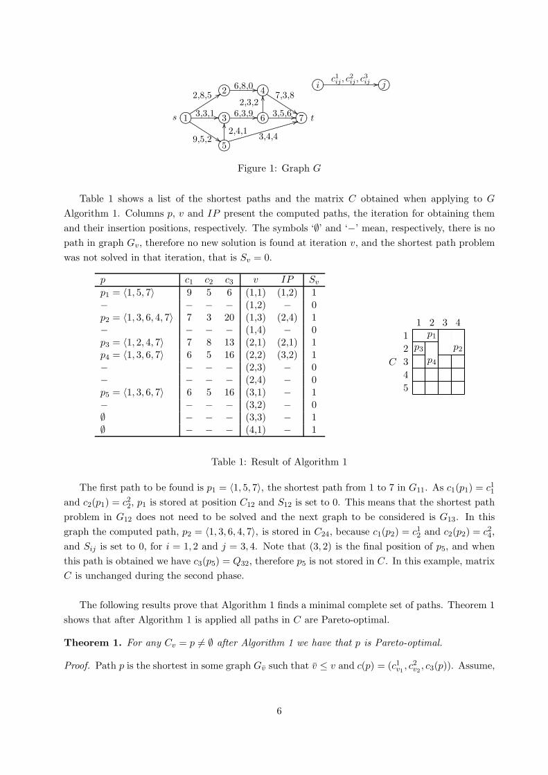
............................................................................................... 1s

............................................................................................... 2

............................................................................................... 3

............................................................................................... 5

............................................................................................... 4

............................................................................................... 6 ........

...............................................................................

........7 t...............

.............................

..............................

......................................................2,8,5

.......................................................................................... ..............3,3,1.................................................................................................................. ...........

...9,5,2

.......................................................................................... ..............6,8,0

.......................................................................................... ..............6,3,9

.................................................................................................................. ..............

7,3,8

........

........

........

........

........

....................

.............. 2,4,1............................

.........................................................

.........................................................

..................................................................... ..............

3,4,4

........

........

........

........

........

....................

..............2,3,2.......................................................................................... ..............3,5,6

............................................................................................... i ........................................

....................................................... j..................................................................................................................................................................... ..............

c1ij , c

2ij , c

3ij

Figure 1: Graph G

Table 1 shows a list of the shortest paths and the matrix C obtained when applying to G

Algorithm 1. Columns p, v and IP present the computed paths, the iteration for obtaining themand their insertion positions, respectively. The symbols ‘∅’ and ‘−’ mean, respectively, there is nopath in graph Gv, therefore no new solution is found at iteration v, and the shortest path problemwas not solved in that iteration, that is Sv = 0.

p c1 c2 c3 v IP Sv

p1 = 〈1, 5, 7〉 9 5 6 (1,1) (1,2) 1− − − − (1,2) − 0p2 = 〈1, 3, 6, 4, 7〉 7 3 20 (1,3) (2,4) 1− − − − (1,4) − 0p3 = 〈1, 2, 4, 7〉 7 8 13 (2,1) (2,1) 1p4 = 〈1, 3, 6, 7〉 6 5 16 (2,2) (3,2) 1− − − − (2,3) − 0− − − − (2,4) − 0p5 = 〈1, 3, 6, 7〉 6 5 16 (3,1) − 1− − − − (3,2) − 0∅ − − − (3,3) − 1∅ − − − (4,1) − 1

C

12345

1 2 3 4p1

p3 p2

p4

Table 1: Result of Algorithm 1

The first path to be found is p1 = 〈1, 5, 7〉, the shortest path from 1 to 7 in G11. As c1(p1) = c11

and c2(p1) = c22, p1 is stored at position C12 and S12 is set to 0. This means that the shortest path

problem in G12 does not need to be solved and the next graph to be considered is G13. In thisgraph the computed path, p2 = 〈1, 3, 6, 4, 7〉, is stored in C24, because c1(p2) = c1

2 and c2(p2) = c24,

and Sij is set to 0, for i = 1, 2 and j = 3, 4. Note that (3, 2) is the final position of p5, and whenthis path is obtained we have c3(p5) = Q32, therefore p5 is not stored in C. In this example, matrixC is unchanged during the second phase.

The following results prove that Algorithm 1 finds a minimal complete set of paths. Theorem 1shows that after Algorithm 1 is applied all paths in C are Pareto-optimal.

Theorem 1. For any Cv = p 6= ∅ after Algorithm 1 we have that p is Pareto-optimal.

Proof. Path p is the shortest in some graph Gv such that v ≤ v and c(p) = (c1v1

, c2v2

, c3(p)). Assume,

6

by contradiction, that there is a path p that dominates p, that is,

c(p) = (c1v1

, c2v2

, c3(p)) ≤ c(p) = (c1v1

, c2v2

, c3(p)) and c(p) 6= c(p).

Then v ≤ v ≤ v, therefore p is also a path in Gv . On the one hand p is the shortest path in thatgraph, and on the other hand c(p) ≥ c(p), thus c3(p) = c3(p). This last equality together withc(p) ≤ c(p) and c(p) 6= c(p) leads to c1

v1< c1

v1or c2

v2< c2

v2.

Let us consider c1v1

< c1v1

(the other case can be treated similarly). Then v ≥ v with v1 > v1,therefore p is a path in Gv+ , where v+ = (v1 +1, v2). Two cases can be considered for iteration v+:

1. If the shortest path problem is solved in Gv+ , the solution is p+ such that c3(p+) ≤ c3(p) =c3(p) and p+ is inserted in Cv, for some v ≥ v+. Furthermore v ≥ v with v1 ≥ v1 + 1, thus inthe second phase, when i = v1 + 1 and j = v2 we have Qij ≤ c3(p+) ≤ c3(p) = Qv = Qi−1j,then Cv is set to ∅.

2. Else in some iteration v1 such that v1 ≤ v+, a path p+ is obtained and inserted in Cv forsome v ≥ v+. We have p in Gv1 because v1 ≤ v+, then c3(p+) ≤ c3(p) = c3(p). Using thesame proof we again conclude that Cv = ∅.

Thus c1v1

< c1v1

implies Cv = ∅, which contradicts Cv = p 6= ∅, therefore p is Pareto-optimal.

Lemma 1 is an auxiliary result for proving Theorem 2.

Lemma 1. A Pareto-optimal path is never deleted from C by Algorithm 1.

Proof. In the first phase a solution p is only replaced by another solution p, when p dominates p.A path p is only deleted in the second phase if p is dominated by another path in C. Therefore aPareto-optimal path is never removed from C.

Theorem 2 shows that after Algorithm 1, for each Pareto-optimal path, the matrix C containsa path with the same objective vector.

Theorem 2. Let p∗ be a Pareto-optimal path and v be such that ck(p∗) = ckvk

, k = 1, 2. After theapplication of Algorithm 1, Cv = p, with p some path in P such that c(p) = c(p∗).

Proof. Two cases have to be analyzed:

1. The shortest path problem in Gv is not solved. In this case a path p is obtained in Gv, wherev ≤ v, and inserted in position v such that v ≥ v. Then ck(p) = ck

vk≤ ck

vk= ck(p∗), k = 1, 2.

Since v ≤ v the path p∗ is in graph Gv, and therefore c3(p) ≤ c3(p∗), hence c(p) ≤ c(p∗). Asp∗ is Pareto-optimal, then c(p) = c(p∗) and v = v. This means p is also Pareto-optimal and,at iteration v, p is stored in Cv.

2. The shortest path problem in Gv is solved. p∗ is a path in graph Gv. If p is the shortestpath obtained at iteration v, then c3(p) ≤ c3(p∗). As v is p∗’s final position and p ∈ Gv,then ck(p) ≤ ck(p∗), k = 1, 2, therefore c(p) ≤ c(p∗). On the other hand p∗ is Pareto-optimal,therefore c(p) = c(p∗) must hold, which implies p is a Pareto-optimal too and v is its finalposition. Finally Cv = p at the end of iteration v.

7

In both cases, by Lemma 1 Cv = p holds.

Therefore the set of paths in C after Algorithm 1 is a minimal complete set of Pareto-optimalsolutions. All solutions are Pareto-optimal (Theorem 1) and for any Pareto-optimal we have a pathin C with the same objective vector (Theorem 2). Moreover, note that the paths in C have distinctobjective vectors. The paths are inserted in the final positions and there is at most one path ineach C position, thus there are no two paths with exactly the same values in c1, c2.

The number of operations performed by Algorithm 1 depends on the number of distinct valuesof the bottleneck objective functions, m1,m2 ≤ m, which are correlated with the number of Pareto-optimal solutions, and thus the number of shortest path problems that have to be solved. As aresult the new method shares the same worst-case complexity order of previous algorithms in theliterature, O(m1m2c(n)), where c(n) is the number of operations needed to find the shortest pathin a network with n nodes. The same bound is valid for the variant that avoids ties in the paths’bottleneck values, as in a worst-case there is a non-dominated solution for every pair of bottleneckvalues c1 and c2.

As for the tricriteria label setting algorithm, each node may have at most m1m2 labels, andthe binary heap used to manage all temporary labels together can have at most nm1m2 elementsin total, which has a time complexity of O(log(nm1m2)). Moreover, in the worst-case, each arc isanalyzed m1m2 times, O(m1m2 log(nm1m2)), and for each the dominance test has to be applied,which takes O(mm2

1m22 log(nm1m2)) time. In the worst-case the label setting algorithm performs

O(mm21m

22 log(nm1m2) + nm1m2 log(nm1m2)) operations.

4 Computational experiments

Computational experiments were carried out to evaluate the performance of the new methods,as well as to compare them with previous approaches. Seven codes were implemented in C: themethods described in the literature, MMS and MMS-R [14, 15], the stair method, MMS-S [17], the blocksmethod, MMS-B, and the label setting algorithm, MMS-LS, as well as the variants of MMS-S and MMS-B

which deal with cost ties, MMS-ST and MMS-BT. The stair method can be seen as a preliminar versionof the blocks method, which still intends to use the objective values of the paths computed to avoidsolving some shortest path problems, but taking into account only one of the objective functionsc1, c2. More details about this method can be found in [17]. In order to determine the shortest path,the first four programs used Dijkstra’s algorithm [6], implemented with a binary heap to managethe temporary labels. The last two used its modified version described in Section 2. MMS-LS wasimplemented with a binary heap too, that manages all temporary labels together. The codes ranon an Intel Core 2 Duo 2.0GHz with 3GB of RAM.

Random networks with 2 000, 7 000, 12 000, 15 000, 20 000 and 30 000 nodes, dn arcs, for densitiesd = 5, 20 and 100, and integer c3

ij uniformly generated in [1,M ], with M = 10, 50, 1 000, wereconsidered. The bottleneck values ck

ij are integers randomly generated in [1,mk], k = 1, 2, wherem1 = m2 may be 20, 100, 500 and 1 000. For any node i, d successors j are randomly chosen andthe arcs (i, j) are created in A. The networks were represented using the forward star form [1].

All the results are average values for 10 different instances of each data set dimension. Tables 2,

8

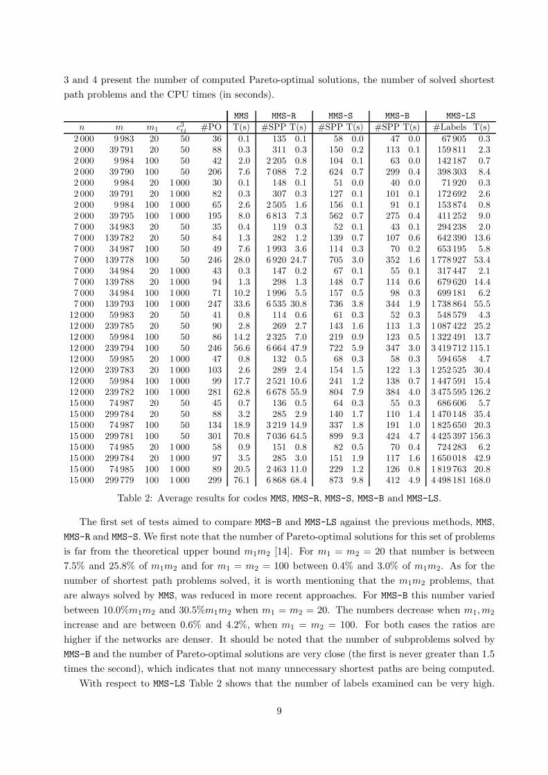
3 and 4 present the number of computed Pareto-optimal solutions, the number of solved shortestpath problems and the CPU times (in seconds).

MMS MMS-R MMS-S MMS-B MMS-LSn m m1 c3

ij #PO T(s) #SPP T(s) #SPP T(s) #SPP T(s) #Labels T(s)2 000 9 983 20 50 36 0.1 135 0.1 58 0.0 47 0.0 67 905 0.32 000 39 791 20 50 88 0.3 311 0.3 150 0.2 113 0.1 159 811 2.32 000 9 984 100 50 42 2.0 2 205 0.8 104 0.1 63 0.0 142 187 0.72 000 39 790 100 50 206 7.6 7 088 7.2 624 0.7 299 0.4 398 303 8.42 000 9 984 20 1 000 30 0.1 148 0.1 51 0.0 40 0.0 71 920 0.32 000 39 791 20 1 000 82 0.3 307 0.3 127 0.1 101 0.1 172 692 2.62 000 9 984 100 1 000 65 2.6 2 505 1.6 156 0.1 91 0.1 153 874 0.82 000 39 795 100 1 000 195 8.0 6 813 7.3 562 0.7 275 0.4 411 252 9.07 000 34 983 20 50 35 0.4 119 0.3 52 0.1 43 0.1 294 238 2.07 000 139 782 20 50 84 1.3 282 1.2 139 0.7 107 0.6 642 390 13.67 000 34 987 100 50 49 7.6 1 993 3.6 114 0.3 70 0.2 653 195 5.87 000 139 778 100 50 246 28.0 6 920 24.7 705 3.0 352 1.6 1 778 927 53.47 000 34 984 20 1 000 43 0.3 147 0.2 67 0.1 55 0.1 317 447 2.17 000 139 788 20 1 000 94 1.3 298 1.3 148 0.7 114 0.6 679 620 14.47 000 34 984 100 1 000 71 10.2 1 996 5.5 157 0.5 98 0.3 699 181 6.27 000 139 793 100 1 000 247 33.6 6 535 30.8 736 3.8 344 1.9 1 738 864 55.5

12 000 59 983 20 50 41 0.8 114 0.6 61 0.3 52 0.3 548 579 4.312 000 239 785 20 50 90 2.8 269 2.7 143 1.6 113 1.3 1 087 422 25.212 000 59 984 100 50 86 14.2 2 325 7.0 219 0.9 123 0.5 1 322 491 13.712 000 239 794 100 50 246 56.6 6 664 47.9 722 5.9 347 3.0 3 419 712 115.112 000 59 985 20 1 000 47 0.8 132 0.5 68 0.3 58 0.3 594 658 4.712 000 239 783 20 1 000 103 2.6 289 2.4 154 1.5 122 1.3 1 252 525 30.412 000 59 984 100 1 000 99 17.7 2 521 10.6 241 1.2 138 0.7 1 447 591 15.412 000 239 782 100 1 000 281 62.8 6 678 55.9 804 7.9 384 4.0 3 475 595 126.215 000 74 987 20 50 45 0.7 136 0.5 64 0.3 55 0.3 686 606 5.715 000 299 784 20 50 88 3.2 285 2.9 140 1.7 110 1.4 1 470 148 35.415 000 74 987 100 50 134 18.9 3 219 14.9 337 1.8 191 1.0 1 825 650 20.315 000 299 781 100 50 301 70.8 7 036 64.5 899 9.3 424 4.7 4 425 397 156.315 000 74 985 20 1 000 58 0.9 151 0.8 82 0.5 70 0.4 724 283 6.215 000 299 784 20 1 000 97 3.5 285 3.0 151 1.9 117 1.6 1 650 018 42.915 000 74 985 100 1 000 89 20.5 2 463 11.0 229 1.2 126 0.8 1 819 763 20.815 000 299 779 100 1 000 299 76.1 6 868 68.4 873 9.8 412 4.9 4 498 181 168.0

Table 2: Average results for codes MMS, MMS-R, MMS-S, MMS-B and MMS-LS.

The first set of tests aimed to compare MMS-B and MMS-LS against the previous methods, MMS,MMS-R and MMS-S. We first note that the number of Pareto-optimal solutions for this set of problemsis far from the theoretical upper bound m1m2 [14]. For m1 = m2 = 20 that number is between7.5% and 25.8% of m1m2 and for m1 = m2 = 100 between 0.4% and 3.0% of m1m2. As for thenumber of shortest path problems solved, it is worth mentioning that the m1m2 problems, thatare always solved by MMS, was reduced in more recent approaches. For MMS-B this number variedbetween 10.0%m1m2 and 30.5%m1m2 when m1 = m2 = 20. The numbers decrease when m1,m2

increase and are between 0.6% and 4.2%, when m1 = m2 = 100. For both cases the ratios arehigher if the networks are denser. It should be noted that the number of subproblems solved byMMS-B and the number of Pareto-optimal solutions are very close (the first is never greater than 1.5times the second), which indicates that not many unnecessary shortest paths are being computed.

With respect to MMS-LS Table 2 shows that the number of labels examined can be very high.

9

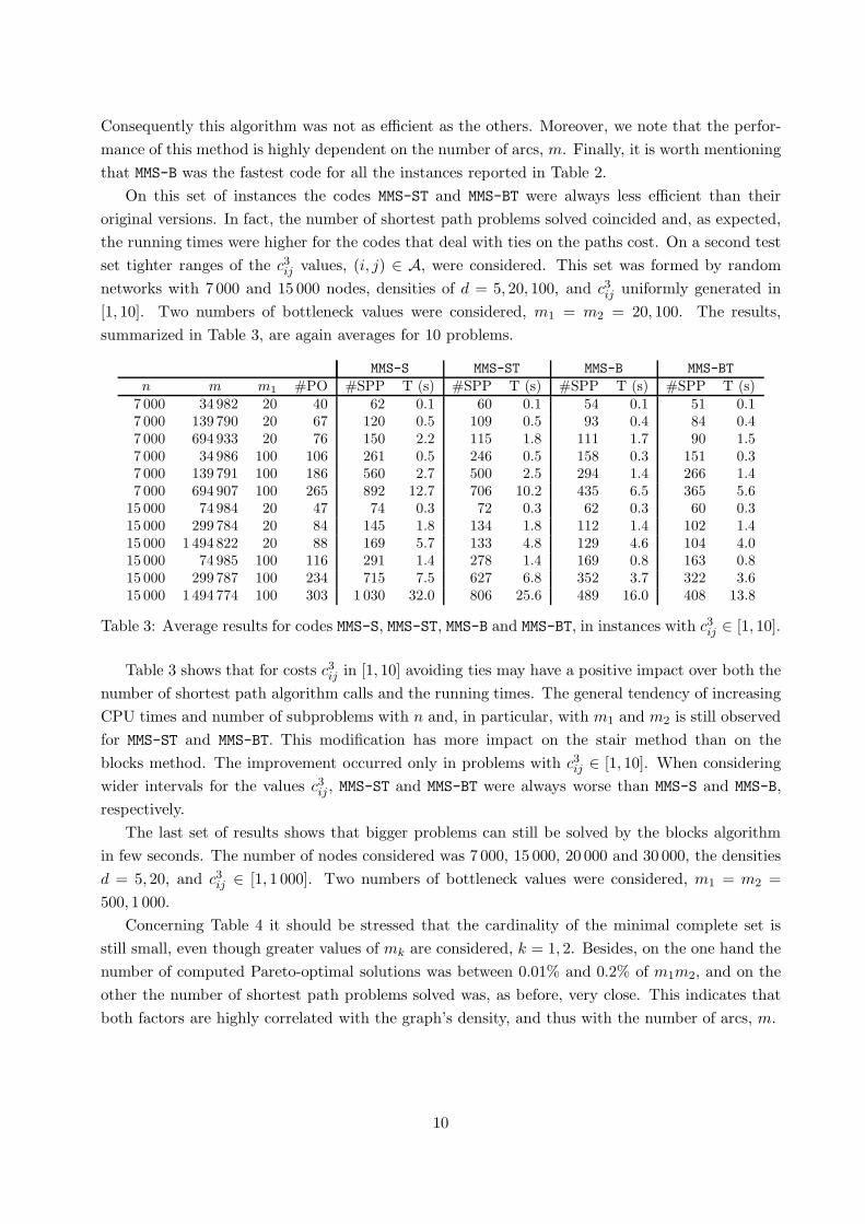
Consequently this algorithm was not as efficient as the others. Moreover, we note that the perfor-mance of this method is highly dependent on the number of arcs, m. Finally, it is worth mentioningthat MMS-B was the fastest code for all the instances reported in Table 2.

On this set of instances the codes MMS-ST and MMS-BT were always less efficient than theiroriginal versions. In fact, the number of shortest path problems solved coincided and, as expected,the running times were higher for the codes that deal with ties on the paths cost. On a second testset tighter ranges of the c3

ij values, (i, j) ∈ A, were considered. This set was formed by randomnetworks with 7 000 and 15 000 nodes, densities of d = 5, 20, 100, and c3

ij uniformly generated in[1, 10]. Two numbers of bottleneck values were considered, m1 = m2 = 20, 100. The results,summarized in Table 3, are again averages for 10 problems.

MMS-S MMS-ST MMS-B MMS-BTn m m1 #PO #SPP T (s) #SPP T (s) #SPP T (s) #SPP T (s)

7 000 34 982 20 40 62 0.1 60 0.1 54 0.1 51 0.17 000 139 790 20 67 120 0.5 109 0.5 93 0.4 84 0.47 000 694 933 20 76 150 2.2 115 1.8 111 1.7 90 1.57 000 34 986 100 106 261 0.5 246 0.5 158 0.3 151 0.37 000 139 791 100 186 560 2.7 500 2.5 294 1.4 266 1.47 000 694 907 100 265 892 12.7 706 10.2 435 6.5 365 5.6

15 000 74 984 20 47 74 0.3 72 0.3 62 0.3 60 0.315 000 299 784 20 84 145 1.8 134 1.8 112 1.4 102 1.415 000 1 494 822 20 88 169 5.7 133 4.8 129 4.6 104 4.015 000 74 985 100 116 291 1.4 278 1.4 169 0.8 163 0.815 000 299 787 100 234 715 7.5 627 6.8 352 3.7 322 3.615 000 1 494 774 100 303 1 030 32.0 806 25.6 489 16.0 408 13.8

Table 3: Average results for codes MMS-S, MMS-ST, MMS-B and MMS-BT, in instances with c3ij ∈ [1, 10].

Table 3 shows that for costs c3ij in [1, 10] avoiding ties may have a positive impact over both the

number of shortest path algorithm calls and the running times. The general tendency of increasingCPU times and number of subproblems with n and, in particular, with m1 and m2 is still observedfor MMS-ST and MMS-BT. This modification has more impact on the stair method than on theblocks method. The improvement occurred only in problems with c3

ij ∈ [1, 10]. When consideringwider intervals for the values c3

ij , MMS-ST and MMS-BT were always worse than MMS-S and MMS-B,respectively.

The last set of results shows that bigger problems can still be solved by the blocks algorithmin few seconds. The number of nodes considered was 7 000, 15 000, 20 000 and 30 000, the densitiesd = 5, 20, and c3

ij ∈ [1, 1 000]. Two numbers of bottleneck values were considered, m1 = m2 =500, 1 000.

Concerning Table 4 it should be stressed that the cardinality of the minimal complete set isstill small, even though greater values of mk are considered, k = 1, 2. Besides, on the one hand thenumber of computed Pareto-optimal solutions was between 0.01% and 0.2% of m1m2, and on theother the number of shortest path problems solved was, as before, very close. This indicates thatboth factors are highly correlated with the graph’s density, and thus with the number of arcs, m.

10

MMS-Bn m m1 #PO #SPP T (s)

7 000 34 986 500 121 179 0.57 000 139 796 500 374 564 3.1

15 000 74 984 500 199 297 1.715 000 299 789 500 434 666 7.920 000 99 985 500 129 195 1.620 000 399 770 500 411 622 9.820 000 100 000 1 000 129 196 1.620 000 400 000 1 000 497 773 11.830 000 150 000 1 000 238 364 4.430 000 600 000 1 000 538 837 19.9

Table 4: Average results for code MMS-B in instances with c3ij ∈ [1, 1 000].

5 Final remarks

We have introduced a method for finding the minimal complete set of Pareto-optimal paths for atricriteria path problem involving two bottleneck objective functions and a cost, the blocks method.This method enhances the procedures presented recently in [14, 15, 17] by using the objective valuesof the obtained paths to reduce the number of shortest path subproblems that have to be solved.As a result the new method has the same worst-case complexity order as previous algorithms,O(m1m2c(n)), where c(n) is the number of operations needed to find the shortest path in a networkwith n nodes. Empirical tests showed that in practice this bound is far from being attained andin random instances with n = 15000, average degree 20 and m1 = m2 = 100 the blocks methodimproved the previous solving about 16 times less shortest path problems than before. As a resultthe CPU times were improved in about 14 times. The blocks method was able to compute theminimal complete set in instances of n = 30000 and m1 = m2 = 1000 in less than 20 seconds.

A variant of the method with the purpose of reducing the number of subproblems that have tobe solved was also proposed. To this end the labeling test used in the shortest path algorithm ismodified so that every time two paths ending at a given node have the same cost, the one with thebest bottleneck value is chosen. For the experiments performed on random instances the percentageof improvement with this variant was at most 15% for arc costs in [1, 10]. A label setting algorithm,with worst-case complexity order of O(mm2

1m22 log(nm1m2)) was also proposed, however the high

number of labels it has to manage led it to a poor performance in the tests performed, whencompared to the others.

Finally, it should be noted that the idea used to develop the blocks method defines a wayto search for the best solutions in matrix C. Therefore it can be applied to other combinatorialproblems with one additive and two bottleneck functions. Moreover this procedure can be extendedto the multi-objective bottleneck network problem, similarly to what was done in [16].

Acknowledgments This work was developed during a visit of L. Pinto and M. Pascoal to CIR-RELT, Montreal, Canada. It was partly supported by Government of Canada, Graduate StudentsExchange Program, by the National Council for Scientific and Technological Development of Brazil(CNPq), and by the FCT Portuguese Foundation of Science and Technology (Fundacao para a

11

Ciencia e a Tecnologia) under grant SFRH/BSAB/830/2008 and project POSC/U308/1.3/NRE/04.The authors also thank Gilbert Laporte for comments and suggestions on a preliminary version ofthis manuscript.

References

[1] Ahuja, R., Magnanti, T., Orlin, J. Network Flows: Theory, Algorithms and Applications.Prentice Hall, Englewood Cliffs, NJ, 1993.

[2] Berman, O., Einav, D., Handler, G. “The constrained bottleneck problem in network”. Oper-ations Research 38, pp. 178-181, 1990.

[3] Brumbaugh-Smith, J. and Shier, D. R. “An empirical investigation of some bicriterion shortestpath algorithms”. European Journal of Operational Research 43, pp. 216-224, 1989.

[4] Clımaco, J., Martins, E. “On the determination of the nondominated paths in a multiobjec-tive network problem”. Proc. of the V Symposium uber Operations Research, Koln, 1980, inMethods in Operations Research, Anton Hain, Konigstein 40, pp. 255-258, 1981.

[5] Clımaco, J., Martins, E. “A bicriterion shortest path algorithm”. European Journal of Opera-tional Research 11, pp. 399-404, 1982.

[6] Dijkstra, E. “A note on two problems in connection with graphs”. Numerical Mathematics 1,pp. 395-412, 1959.

[7] Gandibleux, X., Beugnies, F., Randriamasy. S. “Multi-objective shortest path problems with amaxmin cost function”. 4OR – Quarterly Journal of the Belgian, French and Italian OperationsResearch Societies 4, pp. 47-59, 2006.

[8] Guerriero, F., Musmanno, R., “Label correcting methods to solve multicriteria shortest pathproblems”. Journal of Optimization Theory and Applications 111, pp. 589-613, 2001.

[9] Hansen, P. “Bicriterion path problems”. In: Multicriteria decision making: theory and appli-cations, Lecture Notes in Economics and Mathematical Systems 177, G. Fandel and T. Gal(eds.), Springer, Heidelberg, pp. 109-127, 1980.

[10] Martins, E. “On a multicriteria shortest path problem”. European Journal of OperationalResearch 16, pp. 236-245, 1984.

[11] Martins, E. “On a special class of bicriterion path problems”. European Journal of OperationalResearch 17, pp. 85-94, 1984.

[12] Martins, E., Pascoal, M., Rasteiro, D., Santos, J. “The optimal path problem”. InvestigacaoOperacional 19, pp. 43-60, 1999. (http://www.mat.uc.pt/∼marta/Publicacoes/opath.ps.gz).

[13] Mote, J., Murthy, I., Olson, D. “A parametric approach to solving bicriterion shortest pathproblems”. European Journal of Operational Research 53, pp. 81-92, 1991.

12

[14] Pinto, L., Bornstein, C., Maculan, N. “The tricriterion shortest path problem with at least twobottleneck objective functions”. European Journal of Operational Research 198, pp. 387-391,2009.

[15] Pinto, L., Bornstein, C., Maculan, N. “Um problema de caminho tri-objetivo”. Anais do XLSBPO, Joao Pessoa-PB, pp. 1032-1042, 2008. (http://www.cos.ufrj.br/∼leizer/MMS-R.pdf)

[16] Pinto, L., Bornstein, C., Maculan, N. “A polynomial algorithm for the multi-objective bottle-neck network problem with one MinSum objective function”. Submitted to Networks, 2008.

[17] Pinto, L., Pascoal, M. “Enhanced algorithms for tricriteria shortest path problemswith two bottleneck objective functions”. Technical Report no 3, INESC-Coimbra, 2009.(http://www.inescc.pt/documentos/3 2009.pdf)

[18] Raith, A., Ehrgott, M. “A comparison of solution strategies for biobjective shortest pathproblems”. Computers and Operations Research 36, pp. 1299-1331, 2009.

[19] Skriver, A., Andersen, K. A. “A label correcting approach for solving bicriterion shortest-pathproblems”. Computers and Operations Research 27, pp. 507-524, 2000.

[20] Tung, C., Chew, K. “A multicriteria Pareto-optimal path algorithm”. European Journal ofOperational Research 62, pp. 203-209, 1992.

13

Anexo 3

Este anexo contem o artigo de Pinto e Laporte intitulado An efficient algorithm

for the Steiner tree problem with revenue, bottleneck and hop objective functions, o

qual foi submetido a European Journal of Operational Research. A versao inicial foi

submetida em abril de 2009. Em outubro recebemos as sugestoes dos revisores e as

implementamos na atual versao. Este anexo contem essa nova versao, submetida

em novembro de 2009.

.

58

An efficient algorithm for the Steiner tree problem with revenue, bottleneckand hop objective functions

Leizer Lima Pinto1,2 and Gilbert Laporte2,3

1COPPE/UFRJ - Federal University of Rio de Janeiro, BrazilDepartment of Systems Engineering and Computer Science

E-mail: leizer@cos.ufrj.br

2Interuniversity Research Centre on Enterprise Networks, Logistics and Transportation (CIRRELT)E-mail: Gilbert.Laporte@cirrelt.ca

3Canada Research Chair in Distribution Management, HEC Montreal, 3000 chemin de laCote-Sainte-Catherine, Montreal, Canada H3T 2A7

April 2009Revised November 2009

Abstract

This paper considers a tricriteria Steiner tree problem arising in the design of telecom-munication networks. The objective functions consist of maximizing the revenue and ofminimizing the maximal distance between each pair of interconnected nodes, as well asthe maximal number of arcs between the root and each node. A polynomial algorithmis developed for the generation of a minimal complete set of Pareto-optimal Steinertrees. Optimality proofs are given and computational experience on a set of randomlygenerated problems is reported.

Keywords: Steiner tree; Multi-objective problem; Pareto-optimal solution; Bottleneckfunction.

1 The problem

The classical Steiner Tree Problem (STP) consists of finding a Steiner tree minimizing the sumof its arc costs. This single-objective problem is a well known NP-hard problem in combinatorialoptimization (see [10, 12]). In the Prize-Collecting Steiner Tree Problem (PCSTP) the goal is tofind a Steiner tree maximizing the difference between the collected revenue, equal to the sum ofthe node revenues, and the network cost, equal to the sum of the arc costs. The STP is a paticularcase of the PCSTP in which all the revenues are zero, and therefore the PCSTP is also NP-hard.The PCSTP has been studied in [4, 8, 13, 14].

A variant of the PCSTP which consists of finding a Steiner tree maximizing the revenue underbudget and hop constraints has been studied in Costa et al. [7]. The budget is the networkcost, i.e., the sum of the arc costs. This problem is NP-hard because of the budget constraint.However, changing this constraint to a bottleneck constraint yields a polynomial problem. Here,the bottleneck and the hop are considered as objective functions, instead of constraints. Single-objective bottleneck Steiner tree problems are considered in [5, 16].

The purpose of this paper is to propose a polynomial algorithm for the generation of a minimalcomplete set of Pareto-optimal solutions for a tricriteria Steiner tree problem arising in the designof telecommunication networks. The problem is defined on a directed graph G = (N ,A) with|N | = n and |A| = m. Each arc (i, j) ∈ A has an associated length dij ∈ R and each node i ∈ Nhas an associated revenue ri ≥ 0. Given a set of terminal nodes T ⊆ N , a directed tree G = (V, E)

1

of G with root s ∈ T is called a Steiner tree when V ⊇ T . For each i ∈ V let h(i) be the numberof hops between the root s and i in G. Defining S as the set of all Steiner trees of G, the objectivevector associated with Steiner tree G ∈ S is given by f(G) =

(f1(G), f2(G), f3(G)

)∈ R3, where

f1(G) = maxi∈V{h(i)}, f2(G) = max

(i,j)∈E{dij} and f3(G) =

∑

i∈Vri.

The tricriteria Steiner tree problem with revenue, hop and bottleneck objective functions isthen defined as:

minimize fk(G), k = 1, 2

maximize f3(G)

subject to G ∈ S.

Applications of this problem arise in the design of telecommunications local access networks [4,6, 8, 13], such as the construction of a fiber-optic network to provide broadband Internet connectionsto businesses and residential buildings. Here the graph corresponds to a street map since local accessfiber is typically laid along streets. The nodes of the graph correspond to the street intersectionsand to the locations of buildings. To each node representing a building is associated a potentialrevenue generated by providing telecommunication services to that building. The other nodeshave no associated revenue. The cost of creating or maintaining an arc depends on its length.An arc with a large weight in the solution can cause difficulties with respect to network support.Since telecommunications applications usually consider a probability of service failure (here weassume the same probability for all arcs, as in [7, 11]), then a node with a large number of hopsbetween it and the root is more likely to experience failures. Therefore one may be interestedin simultaneously maximizing the revenue, as well as minimizing the maximal arc length andthe maximal number of hops between the root and any node. Zelikovsky [16] describes severalapplications in which a bottleneck objective is appropriate. One is a location problem in whichhospitals are assigned to potential users by means of arcs. Another application arises in electronicphysical design automation where nets are routed subject to delay minimization. In both casesminimizing a bottleneck objective helps maintain service quality by ensuring that transmission ortravel times remain acceptable in the worst case.

The remainder of this paper is organized as follows. The algorithm is described in Section 2,followed by an example in Section 3. An optimality proof is provided in Section 4 and computationalexperiments are reported in Section 5.

2 Algorithm

Graph G ∈ S dominates G ∈ S whenever fk(G) ≤ fk(G), k = 1, 2, and f3(G) ≥ f3(G) withf(G) 6= f(G). A Steiner tree G ∈ S is Pareto-optimal if it is not dominated by any other Steinertree in S. A set S∗ ⊆ S of Pareto-optimal solutions is a minimal complete set if for each G1, G2 ∈ S∗we have f(G1) 6= f(G2) and for any Pareto-optimal solution G∗ ∈ S there exists G ∈ S∗ so thatf(G) = f(G∗).

Let m1 be the number of different values of dij , (i, j) ∈ A, and suppose they are decreasingorder, i.e., d1 > d2 > · · · > dm1 . Considering Ak = {(i, j) ∈ A | dij ≤ dk}, the subgraph of G,Gk = (N ,Ak) can be defined. It is easy to see that G1 = G.

We first describe Algorithm 1 which is an auxiliary procedure used by our main algorithm.It seeks to determine an optimal Steiner tree G = (V, E), with respect to the revenue objectivefunction, in a subgraph Gi of G with no more than h hops between the root s and any node. The

2

algorithm uses a breadth-first search until it finds all nodes j for which there exists a path with atmost h hops from s to j in Gi. The optimality of the algorithm is guaranted because the revenuesare non-negative. Some auxiliary structure are used, namely F , q, r and Hk, where F is the set ofscanned nodes, i.e., j ∈ F means that l ∈ V, ∀(j, l) ∈ Ai; q is the node being scanned at the currentiteration; r is the sum of the revenues of the nodes in V; and Hk contains the number of arcs froms to k in G. A similar algorithm that spans all nodes, i.e., that finds a spanning tree of G using abreadth-first search, is presented in Gabow and Tarjan [9].

Algorithm 1. Finding a Steiner tree in Gi

Given: Gi, h, T and sDo: V ← {s}, E ← ∅, F ← ∅, q ← s, r ← rs, Hs ← 0 and Hk ←∞, ∀k ∈ N − {s}While Hq < h and F 6= V 6= N Do

For all (q, l) ∈ Ai with Hl =∞ DoHl ← Hq + 1, r ← r + rl, V ← V ∪ {l} and E ← E ∪ {(q, l)}

F ← F ∪ {q}q ← j ∈ V − F such that Hj ≤ Hk, ∀k ∈ V − F

If T ⊆ V Then Return (V, E)Else Return ∅

The complexity of Algorithm 1 is O(n2). In the while loop there are never more than n valuesof q. Of course, for any q the maximum number of nodes l so that (q, l) ∈ Ai is n− 1. Moreover,the choice of q at each iteration of the loop is made in V − F operations, where |V − F| ≤ n.

Let Shi be the set of Steiner trees, with f1 ≤ h, in Gi. The following lemma proves the optimality

of Algorithm 1.

Lemma 1. Let G = (V, E) be the solution obtained by Algorithm 1 applied to Gi for a given h.Then f3(G) ≥ f3(G),∀G = (V, E) ∈ Sh

i .

Proof. After Algorithm 1, V is the set of all nodes j ∈ N such that there exists a path from s to jin Gi with no more than h intermediate arcs. Then T 6⊆ V ⇔ Sh

i = ∅, and when Shi 6= ∅ we have

V ⊆ V,∀G = (V, E) ∈ Shi , which implies f3(G) ≥ f3(G), because rk ≥ 0,∀k ∈ N . Therefore G is

the best solution in Gi with respect to the revenue function and with f1 ≤ h.

We now present an algorithm for finding a minimal complete set of Pareto-optimal solution. Itcontains two phases: Pareto-optimal candidates are found in the first phase and the second phaseeliminates dominated and equivalent solutions. Here C and Q are two (n− 1)×m1 matrices usedto store the solutions obtained by algorithm and their f3 objective values, respectively. They allowthe determination of S∗ and its objective vectors. A binary matrix R of dimension (n − 1) ×m1

marks the iterations (subproblems) that have to be executed. Algorithm 1 is called at iterationv = (v1, v2) of Algorithm 2 if and only if Rv = 1; otherwise the next iteration is considered. Variablectrl is used to skip subproblems that have no solution.

The first phase consists of two loops. The indices associated with the outer v1-loop and theinner v2-loop define, respectively, which h and which subgraph, Gv2 , should to be considered byAlgorithm 1 at iteration v = (v1, v2). If a solution G is obtained at iteration v, then it is insertedin Cv, where v is such that f1(G) = n− v1 and f2(G) = dv2 . The value f3(G) is inserted in Qv, andRv is set to 0 for every v such that v ≤ v ≤ v. In the second phase the matrix Q is used to comparethe solutions obtained during the first phase and then, the dominated and equivalent solutions areeliminated from matrix C.

Algorithm 2 is similar to the Blocks algorithm presented by Pinto and Pascoal [15] for tricriteriashortest path problems.

3

Algorithm 2. Finding a minimal complete set of Pareto-optimal Steiner treesFor i = 1, . . . , n− 1 Do

For j = 1, . . . ,m1 Do Cij ← ∅, Qij ← −∞ and Rij ← 1ctrl← m1 and v1 ← 1Phase 1. Finding Pareto-optimal candidatesWhile v1 ≤ n− 1 and ctrl 6= 0 Do

v2 ← 1While v2 ≤ ctrl Do

If Rv = 1 ThenG← the result of Algorithm 1 for Gv2 , h = n− v1, T and sIf G = ∅ Then ctrl← v2 − 1Else

v1 ← n− f1(G) and v2 ← g such that f2(G) = dg

If f3(G) > Qv ThenCv ← G and Qv ← f3(G)For i = v1, . . . , v1 Do

For j = v2, . . . , v2 Do Rij ← 0v2 ← v2 + 1

v1 ← v1 + 1Phase 2. Filtering Pareto-optimal solutions in CFor i = n− 1, . . . , 1 Do

For j = m1, . . . , 1 DoIf Qij 6= −∞ Then

If j > 1 and Qij ≥ Qij−1 Then Cij−1 ← ∅, Qij−1 ← Qij

If i > 1 and Qij ≥ Qi−1j Then Ci−1j ← ∅, Qi−1j ← Qij

The complexity of Algorithm 2 is O(m1n3). The number of iteration in Phase 1 is no more

than (n− 1)m1. The complexity of each iteration is O(n2), which is the complexity of Algorithm1. Thus the complexity of Phase 1 is O(m1n

3). It is easy to see that the complexity of Phase 2

is O(m1n).Naturally, we always have v ≤ v in Algorithm 2, where v is the insertion position, in C, of

the Steiner tree G obtained at iteration v. By Algorithm 1 f1(G) ≤ h = n − v1, implying thatv1 ≤ n − f1(G) = v1. Since G = (V, E) was obtained in Gv2 = (N ,Av2) then E ⊆ Av2 leading todv2 = f2(G) ≤ dv2 , which implies that v2 ≤ v2.

3 Example

To illustrate Algorithm 2, we apply it to graph G depicted in Figure 1. For this instance m1 = 5with dij ∈ {9, 8, 4, 3, 1}, for any (i, j) ∈ A.

............................................................................................... 1

0

............................................................................................... 2

10

............................................................................................... 3

27

............................................................................................... 5

18

............................................................................................... 4

15

............................................................................................... 6

5...............................................................................................7

20

...............................................................................................8

12

...............................................................................................9

0

...............................................................................................10

0

............................

............................

............................

............................................

9.......................................................................................... ..............1.................................................................................................................. ...........

...3

.......................................................................................... ..............4

.......................................................................................... ..............3

.................................................................................................................. ..............

1................................................................................................................................................................................................... ..............8

........

........

........

........

........

....................

..............4............................

........................................................

........................................................

........................................................

............... ..............

3................................................................................................................................................................................................... ..............

1

........

........

........

........

........

....................

..............9.......................................................................................... ..............8

..........................................................................

1

............................

............................

............................

............................................

9

.......................................................................................... ..............9

............................

............................

............................

............................................

9

..........................................................................3

............................................................................................... i

ri........................................

....................................................... j

rj

....................................................................................................................................... ..............dij

Figure 1: Graph G.

4

We consider T = {s = 1, 3, 7, 8}. Figures 2, 3 and 4 depict the solutions obtained in Phase 1.These figures contain the subgraph Gv2 at iteration v, the Steiner tree obtained by Algorithm 1 inGv2 and the updates made at the end of these iterations.

............................................................................................... 1

G1........................................

....................................................... 2

............................................................................................... 3

............................................................................................... 5

............................................................................................... 4

............................................................................................... 6 ........

...............................................................................

........7

...............................................................................................8

...............................................................................................9

...............................................................................................10

............................

............................

............................

............................................

.......................................................................................... ................................................................................................................................ ...........

...

.......................................................................................... ..............

.......................................................................................... ..............

.................................................................................................................. ..............

................................................................................................................................................................................................... ..............

........

........

........

........

........

....................

..............

........................................................

........................................................

........................................................

........................................... ..............

................................................................................................................................................................................................... ..............

........

........

........

........

........

....................

..............

.......................................................................................... ..............

..........................................................................

............................

............................

............................

............................................

.......................................................................................... ..............

............................

............................

............................

............................................

..........................................................................

............................................................................................... 1

S1 = G ............................................................................................... 2

............................................................................................... 3

............................................................................................... 5

............................................................................................... 4

............................................................................................... 6 ........

...............................................................................

........7

...............................................................................................8

...............................................................................................9

...............................................................................................10

............................

............................

............................

............................................

.......................................................................................... ................................................................................................................................ ...........

...

.......................................................................................... ..............

.......................................................................................... ..............

................................................................................................................................................................................................... ..............

........................................................

........................................................

........................................................

........................................... ..............

................................................................................................................................................................................................... ..............

.......................................................................................... ..............

v1 ← 10− 3, v2 ← 1, C71 ← S1, Q71 ← 107 and Rij ← 0, for 1 ≤ i ≤ 7 and j = 1.

Figure 2: First iteration, h = 9 and v = (1, 1).

............................................................................................... 1

G2........................................

....................................................... 2

............................................................................................... 3

............................................................................................... 5

............................................................................................... 4

............................................................................................... 6 ........

...............................................................................

........7

...............................................................................................8

...............................................................................................9

...............................................................................................10.......................................................................................... ..............

.................................................................................................................. ..............

.......................................................................................... ..............

.......................................................................................... ..............

.................................................................................................................. ..............

................................................................................................................................................................................................... ..............

........

........

........

........

........

....................

..............

........................................................

........................................................

........................................................

........................................... ..............

................................................................................................................................................................................................... ..............

.......................................................................................... ..............

..........................................................................

..........................................................................

............................................................................................... 1

S2 = G

............................................................................................... 3

............................................................................................... 5

............................................................................................... 6 ........

...............................................................................

........7

...............................................................................................8

.......................................................................................... ................................................................................................................................ ...........

...

.......................................................................................... ..............

........................................................

........................................................

........................................................

........................................... ..............

................................................................................................................................................................................................... ..............

v1 ← 10− 2, v2 ← 4, C84 ← S2, Q84 ← 82 and Rij ← 0, for 1 ≤ i ≤ 8 and 2 ≤ j ≤ 4.

Figure 3: Second iteration, h = 9 and v = (1, 2).

At iterations three, v = (1, 3), and four, v = (1, 4), we have Rv = 0. The next iteration withRv = 1 is v = (1, 5), where A5 = {(1, 3), (4, 7), (5, 8), (7, 8)} ⇒ G = ∅ ⇒ ctrl ← v2 − 1 = 4. This,together with the updates made at iterations (1, 1) and (1, 2), implies that the next iteration withv2 ≤ ctrl and Rv = 1 is v = (8, 1).

............................................................................................... 1

G1........................................

....................................................... 2

............................................................................................... 3

............................................................................................... 5

............................................................................................... 4

............................................................................................... 6 ........

...............................................................................

........7

...............................................................................................8

...............................................................................................9

...............................................................................................10

............................

............................

............................

............................................

.......................................................................................... ................................................................................................................................ ...........

...

.......................................................................................... ..............

.......................................................................................... ..............

.................................................................................................................. ..............

................................................................................................................................................................................................... ..............

........

........

........

........

........

....................

..............

........................................................

........................................................

........................................................

........................................... ..............

................................................................................................................................................................................................... ..............

........

........

........

........

........

....................

..............

.......................................................................................... ..............

..........................................................................

............................

............................

............................

............................................

.......................................................................................... ..............

............................

............................

............................

............................................

..........................................................................

............................................................................................... 1

S3 = G ............................................................................................... 2

............................................................................................... 3

............................................................................................... 5

............................................................................................... 4

............................................................................................... 6 ........

...............................................................................

........7

...............................................................................................8

............................

............................

............................

............................................

.......................................................................................... ................................................................................................................................ ...........

...

.......................................................................................... ..............

.......................................................................................... ..............

........................................................

........................................................

........................................................

........................................... ..............

................................................................................................................................................................................................... ..............

v1 ← 10− 2, v2 ← 1, C81 ← S3, Q81 ← 107 and R81 ← 0.

Figure 4: Iteration v = (8, 1) and h = 2.

At iterations v = (8, 2), (8, 3) and (8, 4) we have Rv = 0. At iteration v = (9, 1), since h = 1then G = ∅ ⇒ ctrl← v2− 1 = 0. This leads at the end of the Phase 1 . Figure 5 shows the matrixC after Phase 2 , i.e., the final result of Algorithm 2.

4 Optimality proof

We now provide the optimality proof of Algorithm 2, i.e., we prove that it can find a minimalcomplete set of Pareto-optimal solutions. We will first show that all Steiner trees in C are Pareto-

5

C

123456789

1 2 3 4 5

S1

S3 S2

Figure 5: Matrix C after Phase 2 of Algorithm 2.

optimal solutions after the execution of Algorithm 2.

Theorem 1. If Cv = G 6= ∅ after Algorithm 2, for any v, then G is a Pareto-optimal solution.

Proof. By Algorithm 2 f1(G) = n − v1 and f2(G) = dv2 . The proof is by contradiction. Supposethat G is not a Pareto-optimal solution. This implies that G is dominated by some G ∈ S, i.e.,fk(G) ≤ fk(G), k = 1, 2, and f3(G) ≥ f3(G), with f(G) 6= f(G). We have f1(G) = n − v1 andf2(G) = dv2 for some v so that 1 ≤ v1 ≤ n− 1 and 1 ≤ v2 ≤ m1. Then n− v1 = f1(G) ≤ f1(G) =n − v1 ⇒ v1 ≥ v1 and dv2 = f2(G) ≤ f2(G) = dv2 ⇒ v2 ≥ v2, so v ≥ v. It can be seen thatf2(G) = dv2 ensures that G is in Gg, for all g ≤ v2. By the analysis presented after the descriptionof Algorithm 2, v ≥ v, where v is the iteration at which G was obtained. Therefore v ≥ v ≥ v,implying that G is also in Gv2 and f1(G) ≤ n − v1. Lemma 1 applied at iteration v of Algorithm2 guarantees that f3(G) ≥ f3(G). On the other hand f3(G) ≤ f3(G), so that f3(G) = f3(G). Thelatter equality together with f(G) 6= f(G) means that fk(G) < fk(G), for some k ∈ {1, 2}. Considerf1(G) < f1(G) (the other case is similar). Then f1(G) = n − v1 ≤ n − (v1 + 1). This inequalitytogether with v2 ≤ v2 guarantees that the Steiner tree G can be found at iteration v+ = (v1 +1, v2).Thus if iteration v+ is executed (Rv+ = 1), the optimality of Algorithm 1 applied to this iterationresults in G, so that f3(G) ≥ f3(G) = f3(G). We have v ≥ v+, where v is the insertion position ofG. Since f3(G) ≥ f3(G), v1 ≥ v1 + 1 and v2 ≥ v2, then, in Phase 2 of Algorithm 2 when i = v1 + 1and j = v2 we have Qij ≥ Qv = f3(G) ≥ f3(G) = Qv = Qi−1j , which implies in Cv = ∅, leadingto a contradiction. Now suppose that iteration v+ is not executed (Rv+ = 0). This means that atsome iteration u such that u ≤ v+, a solution equivalent to G is obtained, i.e., with an f3 valueand an insertion position greater than or equal to f3(G) and v+, respectively. As above, Cv = ∅.Therefore G is a Pareto-optimal solution.

The next result shows that after Algorithm 2, the set of Steiner trees in C contains distinctobjective vectors.

Lemma 2. For any Steiner trees G and G in C obtained after Algorithm 2, we have f(G) 6= f(G).

Proof. Consider v and v, v 6= v, such that Cv = G and Cv = G. By Algorithm 2, f1(G) = n− v1,f1(G) = n− v1, f2(G) = dv2 and f2(G) = dv2 . Of course, fk(G) = fk(G)⇔ vk = vk, k = 1, 2. Butv 6= v and, therefore, f(G) 6= f(G).

Lemma 3. During Algorithm 2 a Pareto-optimal solution is never deleted from matrix C.

6

Proof. During Phase 1 a solution G is only replaced by another solution G if G is dominated by G.Now consider Phase 2. If it has executed Cv ← ∅, where Cv = G 6= ∅ before this update, then wehave Cv = G 6= ∅ with f3(G) ≥ f3(G), for some v ≥ v and v 6= v. By Algorithm 2, f1(G) = n− v1,f1(G) = n− v1, f2(G) = dv2 and f2(G) = dv2 . Since v ≥ v, with v 6= v, then n− v1 ≤ n− v1 anddv2 ≤ dv2 with at least one of the inequalities is strict, leading to fk(G) ≤ fk(G), k = 1, 2, withf1(G) < f1(G) or f2(G) < f2(G). Then fk(G) ≤ fk(G), k = 1, 2, f3(G) ≥ f3(G) and f(G) 6= f(G),which means that G is dominated by G. Therefore a Pareto-optimal is never deleted from C.

The next theorem states that for each Pareto-optimal solution, the matrix C after Algorithm 2contains one solution associated with the same objective vector.

Theorem 2. Let G∗ be any Pareto-optimal solution. After Algorithm 2 we have Cv = G withf(G) = f(G∗), where v is such that f1(G∗) = n− v1 and f2(G∗) = dv2.

Proof. Graph G∗ can be found at iteration v. Then, if this iteration is executed (Rv = 1), Lemma1 ensures that the algorithm will find, at iteration v, a solution G such that f3(G) ≥ f3(G∗).Moreover f2(G) ≤ dv2 = f2(G∗) and f1(G) ≤ n− v1 = f1(G∗), because G was obtained in Gv2 withh = n−v1. Therefore fk(G) ≤ fk(G∗), k = 1, 2 and f3(G) ≥ f3(G∗), but since G∗ is Pareto-optimal,then necessarily f(G) = f(G∗). This equality implies that G is also Pareto-optimal and v is exactlythe G’s insertion position. Therefore, by Lemma 3, after Algorithm 2 we have Cv = G. If iterationv is not executed (Rv = 0), then we have found, at some previous iteration v ≤ v, a solution G withinsertion position v ≥ v. Since v ≤ v then G∗ can be find at iteration v, and thus, by Lemma 1,f3(G) ≥ f3(G∗). The insertion position of G is v ≥ v, then f1(G) = n− v1 ≤ n− v1 = f1(G∗) andf2(G) = dv2 ≤ dv2 = f2(G∗). Thus, as above, f(G) = f(G∗), implying that G is a Pareto-optimalsolution and v = v, which means that Cv = G after iteration v of Phase 1. But, by Lemma 3, Gis never deleted from Cv, so that at the end of Algorithm 2 we have f(Cv) = f(G∗).

These results show that the set of Steiner trees given by C represents a minimal complete setof Pareto-optimal solutions. All solutions are Pareto-optimal (Theorem 1), each one is associatedwith a different objective vector (Lemma 2) and, for any Pareto-optimal, we have an equivalentsolution in C, i.e., with the same objective vector (Theorem 2).

5 Computational experiments

The algorithm just described was implemented in C and ran on an Intel Core 2 Duo 2.0GHz with3GB of RAM. In order to evaluate the performance of Algorithm 2, we present computationalresults on a set of randomly generated problems. These problems was generated as in Beasley [3],following the scheme outlined by Aneja [2]. They are defined by n = |N | = 2 500, 7 000, 13 000and 20 000; |T | = n/100, n/10 and n/4; and, average node degree equal to 4, 10 and 50. Firsta random spanning tree over N is generated, which guarantees that each instance corresponds toa connected graph. Then, additional random arcs are added to A. For each (i, j) ∈ A we have(j, i) ∈ A with dij = dji. The set of terminal nodes T is randomly generated. For revenues ri andlengths dij , integers were generated according to uniform distributions on the interval [1, 100]. Thenetworks are represented using the forward star form (see Ahuja et al. [1]).

Table 1 provides the cardinality (#PO) of the minimal complete set of Pareto-optimal solutions,the number of iterations at which Rv = 1, i.e., how many times Algorithm 1 is called by Algorithm2, and the CPU times in seconds. Values are averages over ten instances.

7

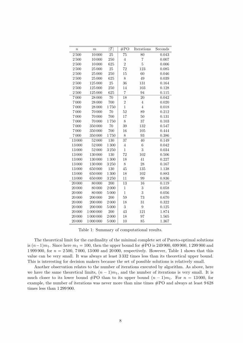
n m |T | #PO Iterations Seconds2 500 10 000 25 75 80 0.0432 500 10 000 250 4 7 0.0072 500 10 000 625 2 5 0.0062 500 25 000 25 72 123 0.0852 500 25 000 250 15 60 0.0462 500 25 000 625 8 49 0.0392 500 125 000 25 36 131 0.1642 500 125 000 250 14 103 0.1282 500 125 000 625 7 94 0.1157 000 28 000 70 18 20 0.0427 000 28 000 700 2 4 0.0207 000 28 000 1 750 1 4 0.0187 000 70 000 70 52 89 0.2127 000 70 000 700 17 50 0.1317 000 70 000 1 750 8 37 0.1037 000 350 000 70 39 132 0.5477 000 350 000 700 16 105 0.4447 000 350 000 1 750 8 93 0.38613 000 52 000 130 37 40 0.14913 000 52 000 1 300 4 6 0.04213 000 52 000 3 250 1 3 0.03413 000 130 000 130 72 102 0.50613 000 130 000 1 300 18 41 0.22713 000 130 000 3 250 8 28 0.16713 000 650 000 130 45 135 1.13813 000 650 000 1 300 18 102 0.88313 000 650 000 3 250 11 99 0.83620 000 80 000 200 13 16 0.11920 000 80 000 2 000 1 3 0.05820 000 80 000 5 000 1 3 0.05620 000 200 000 200 59 73 0.67020 000 200 000 2 000 18 31 0.32220 000 200 000 5 000 3 9 0.12520 000 1 000 000 200 43 121 1.87420 000 1 000 000 2 000 18 97 1.56520 000 1 000 000 5 000 10 85 1.367

Table 1: Summary of computational results.

The theoretical limit for the cardinality of the minimal complete set of Pareto-optimal solutionsis (n−1)m1. Since here m1 = 100, then the upper bound for #PO is 249 900, 699 900, 1 299 900 and1 999 900, for n = 2 500, 7 000, 13 000 and 20 000, respectively. However, Table 1 shows that thisvalue can be very small. It was always at least 3 332 times less than its theoretical upper bound.This is interesting for decision makers because the set of possible solutions is relatively small.

Another observation relates to the number of iterations executed by algorithm. As above, herewe have the same theoretical limits, (n − 1)m1, and the number of iterations is very small. It ismuch closer to its lower bound #PO than to its upper bound (n − 1)m1. For n = 13 000, forexample, the number of iterations was never more than nine times #PO and always at least 9 628times less than 1 299 900.

8

6 Conclusions

In this paper we have developed a polynomial algorithm for a tricriteria Steiner tree problem arisingin the design of telecommunication networks. To our knowledge, this tricriteria problem has neverbeen treated in the operational research literature. Our computational experiments show that largeinstances of this problem can be quickly solved by our algorithm. Instances with 20 000 nodes and1 000 000 arcs were solved in less than two seconds. Additional constraints can be considered in thistricriteria problem. The problem is still easily solved if additional hop and bottleneck constraintsare incorporated: f1 ≤ α and f2 ≤ β, respectively, where α, β ∈ Z+ with α < n − 1 and β < d1.For this first constraint it is just necessary to change, in the initialization of Algorithm 2, v1 ← 1to v1 ← α, so that n − α = α. For the second constraint, arcs (i, j) with dij > β should to bedeleted from G before Algorithm 2 starts.

Acknowledgments This work was partly supported by Government of Canada, Graduate Stu-dents Exchange Program, by the National Council for Scientific and Technological Development ofBrazil (CNPq), and by the Canadian Natural Sciences and Engineering Research Council undergrant 39682-05. This support is gratefully acknowledged. Finally, thanks are due to the refereesfor their valuable comments.

References

[1] Ahuja, R.K., Magnanti, T.L., Orlin, J.B. “Network Flows: Theory, Algorithms and Applica-tions”. Prentice Hall, Englewood Cliffs, New Jersey, 1993.

[2] Aneja Y.P. “An integer linear programming approach to the Steiner problem in graphs”. Net-works 10, 167–178, 1980.

[3] Beasley J.E. “An SST-based algorithm for the Steiner problem in graphs”. Networks 19, 1–16,1989.

[4] Canuto, S.A., Resende, M.G.C., Ribeiro, C.C. “Local search with perturbations for the prize-collecting Steiner tree problem in graphs”, Networks 38, 50–58, 2001.

[5] Chapovska, O., Punnen, A.P. “Variations of the prize-collecting Steiner tree problem”. Networks47, 199–205, 2006.

[6] Costa, A.M., Cordeau, J.-F., Laporte, G. “Steiner tree problems with profits”. INFOR 44,99–115, 2006.

[7] Costa, A.M., Cordeau, J.-F., Laporte, G. “Models and branch-and-cut algorithms for the Steinertree problem with revenues, budget and hop constraints”. Networks 53, 141–159, 2008.

[8] Cunha, A.S., Lucena, A., Maculan, N., Resende, M.G.C. “A relax-and-cut algorithm for theprize-collecting Steiner problem in graphs”. Discrete Applied Mathematics 157, 1198–1217, 2009.

[9] Gabow, H.N., Tarjan, R.E. “Algorithms for two bottleneck optimization problems”. Journal ofAlgorithms 9, 411–417, 1988.

[10] Garey, M.R., Graham, R.L., Johnson, D.S. “The complexity of computing Steiner minimaltrees”. SIAM Journal on Applied Mathematics 32, 835–859, 1977.

[11] Gouveia, L. “Multicommodity flow models for spanning trees with hop constraints”. EuropeanJournal of Operational Research 95, 178–190, 1996.

9

[12] Hakimi, S.L. “Steiner’s problem in graphs and its implications”. Networks 1, 113–133, 1971.

[13] Johnson, D.S., Minkoff, M., Phillips, S. “The prize collecting Steiner tree problem: theoryand practice”. Proceedings of the 11th ACM-SIAM Symposium on Discrete Algorithms, SanFrancisco, 2000.

[14] Lucena, A., Resende, M.G.C. “Strong lower bounds for the prize-collecting Steiner problem ingraphs”. Discrete Applied Mathematics 141, 277–294, 2004.

[15] Pinto, L.L., Pascoal, M. “Enhanced algorithms for tricriteria shortest path problems with twobottleneck objective functions”. Submitted to Computers & Operations Research, 2009.

[16] Zelikovsky, A. “Bottleneck Steiner Tree Problems”. In: Encyclopedia of Optimization, 2ndedition, C. A. Floudas and P. M. Pardalos (Eds.), Springer, New York, 311–313, 2009.

10

Anexo 4

Este anexo contem o artigo de Pinto, Bornstein e Maculan intitulado A polyno-

mial algorithm for the multi-objective bottleneck network problem with one MinSum

objective function, o qual foi submetido a Networks em dezembro de 2008.

69

1

A polynomial algorithm for the multi-objective bottleneck network problem with one

MinSum objective function

Leizer de Lima Pinto

Cláudio Thomás Bornstein

Nelson Maculan*

COPPE/UFRJ – Federal University of Rio de Janeiro, Brazil

Dept. of Systems Engineering and Computer Science

Abstract: The paper presents multi-objective combinatorial optimization problems in graphs where at

most one objective is a MinSum function and the other objectives are of the bottleneck type. A

polynomial algorithm is developed which generates a minimal complete set of Pareto-optimal

solutions. Optimality proofs are given.

Keywords: Multi-objective combinatorial optimization in graphs; Pareto-optimal solution; Bottleneck

problem; Polynomial algorithm.

1) Introduction:

Combinatorial optimization problems in graphs generally consider two kinds of objective

functions. The first can be called a totalizing function and involves the whole set of weights of

arcs/nodes of a feasible solution. The best known example of this function is the MinSum function,

where the objective is to minimize the sum of the weights of arcs of a path or a tree of a graph. Other

possibilities are MaxSum, MinProd, MaxProd, etc.

The second kind of objective function, called a bottleneck function, considers just the

maximum or the minimum weight of the solution. For example, a MinMax bottleneck function will try

to find the path or tree whose arc with maximum weight is minimized. Another possibility is the

MaxMin function. MaxMax and MinMin are of no significance for obvious reasons.

Here, a multi-objective problem will be examined where at most one objective is a totalizing

function. All the other objectives are of the bottleneck type. Ehrgott and Gandibleux [9] present more

than two hundred references in multi-objective combinatorial optimization. The reason for restricting

the number of totalizing functions to one is that the generation of a minimal complete set of Pareto-

optimal solutions for the shortest path, assignment and spanning tree multi-objective problems with

more than one MinSum function is NP-complete (see Serafini [16] and Camerini et al [4]). Azevedo

and Martins [1], Clímaco and Martins [5], Corley and Moon [6], Guerriero and Musmanno [11],

Martins [13] and Tung and Chew [17] present non-polynomial algorithms for the multi-objective

shortest path problem (MSPP) with more than one MinSum objective. Gandibleux et al [10] include a

bottleneck function extending the algorithm presented by Martins [13].

Polynomial algorithms are presented by Hansen [12], Martins [14] and Berman et al [3] for the

bicriterion MinMax-MinSum and by Pinto et al [15] for the tricriterion MaxMin-MinMax-MinSum

shortest path problems. In both cases the goal is the generation of a minimal complete set of Pareto-

optimal solutions.

Applications for the MSPP are given in Batta and Chiu [2], Current and Min [7] and Current

and Marsh [8]. In Pinto et al [15] a tri-objective road transportation problem is presented, where the

two bottleneck functions are associated with road quality and traffic density and cost minimization

stands for the totalizing function.

*Corresponding author. E-mail Address: maculan@cos.ufrj.br. Federal University of Rio de Janeiro,

COPPE/UFRJ, Dept. of Systems Engineering. P.O. Box 68511, 21941-972 Rio de Janeiro, RJ, Brazil.

2

Another possible application for the tri-objective shortest path problem is within

communication networks. A sensor network may be represented by a graph and weights ( )jip ,1 ,

( )jip ,2 and ( )jip ,3 may be associated to each arc ( )j,i . ( )jip ,1 and ( )jip ,2 may represent the

amount of available battery power and the average waiting time at node i respectively. ( )jip ,2 is a

measure of overload of the system and represents the time between the in- and outflow of information

from node i. ( )jip ,3 measures the transmission cost from i to j. A company may be interested in

finding a route from a certain source s to a sink t so that the minimum battery power available at nodes

of the route is maximized, maximum waiting time and total cost of the route are minimized. This

corresponds to a MaxMin-MinMax-MinSum problem.

In this paper a polynomial algorithm will be presented for a graph optimization problem in

which one objective is a MinSum function and the other l objectives are of the MinMax type. The

algorithm here differs considerably from the MMS algorithm presented by Pinto et al [15]. First,

trivially, l+1 objectives instead of just three are considered. Second, and more important, the

algorithm presented in this paper is of a different type. In Pinto et al [15] spanning subgraphs are

generated successively at each iteration in an order of increasing density. Here, on the contrary,

spanning subgraphs are produced in an order of decreasing density. The advantage is that the non-

availability of a path in a certain iteration of a certain loop makes it possible to skip the following

iterations of this loop.

The third improvement presented in this paper concerns the set of restrictions. While in Pinto et

al [15] a feasible solution is a path between two given nodes, here we handle a more general problem.

Like Berman et al [3] given a graph ( )MNG ,= it is just necessary that a feasible solution Ms ⊆

satisfies some property α . As long as a polynomial algorithm is available to optimize the single-

objective problem with a totalizing function, the corresponding multi-objective problem will be solved

in polynomial time.

Section two of the present paper presents some basic definitions, the notation and the MMS-R

algorithm. Section three contains the optimality proofs, showing that the MMS-R algorithm does in

fact generate a minimal complete set. Section four, the conclusions, gives a brief description of the

computational performance of the MMS-R algorithm and some generalizations and extensions. As to

our knowledge no exact polynomial algorithm is mentioned in the literature for the multi-objective

graph optimization problem. Therefore, no comparison of computational efficiency is possible.

However, a comparison of the performances of the MMS and MMS-R algorithms is made for the

tricriterion shortest path problem.

2) Problem and algorithm:

Consider graph ( )MNG ,= with n|N| = and m|M| = . For each arc ( ) Mji ∈, let

( ) 121 +=ℜ∈ l,,,k,j,ip kK , be the k-th weight. Without any loss of generality suppose that the km

different values of ( ).p k in M are arranged in decreasing order, i.e.

k

m

kk

kppp >>> K21 , for

lk ,,2,1 K= .

Let ( )kvv = be an l-dimensional vector of indexes, where kk mv ≤≤1 . Considering

( ) ( ){ }l,,,k,pj,ipMj,iM k

v

k

v kK21=≤∈= leads to ( )vv MNG ,= as a spanning subgraph of G.

Remark that if v is so that { }lkvk ,,2,1,1 K∈∀= then GGv = .

Let Ms ⊆ be a feasible solution satisfying some property α . For example, s may be a

spanning tree or a path between two nodes of G. Let S be the set of all feasible solutions. The

following multi-objective problem can be defined:

3

( )( )

( ){ }

( )( )

.Ss

j,ip

l,,,k,j,ipP

sj,i

l

k

sj,i

∈

=

∑∈

+

∈

:subject to

minimize

21maxminimize

1

K

The first l objectives are of the MinMax type for the sake of simplicity. Any combination of

MinMax or MaxMin will lead to the same kind of algorithm. Using MaxMin instead of MinMax leads

to a reordering of weights.

Next, the definition of Pareto-optimal solution and minimal complete set is given. Let

( ) 1+ℜ∈= ls

k

sqq be the objective vector associated with Ss ∈ , where

( )( ){ } l,,,kj,ipq k

sj,i

s

k K21formax ==∈

and ( )( )∑

∈

+

+ =sj,i

ls

l j,ipq1

1 . We say that Ss ∈ dominates

Ss ∈ when ss qq ≤ with

ss qq ≠ . A solution Ss ∈ is Pareto-optimal if there is no Ss ∈ that

dominates s. A set SS* ⊆ of Pareto-optimal solutions is a minimal complete set if for each two

solutions *

S"s,'s ∈ we have "s's qq ≠ and for any Pareto-optimal solution Ss ∈ there exists

*Ss ∈ so that ss qq = .

The MMS-R algorithm generates a minimal complete set *

S of Pareto-optimal solutions for

problem ( )P . In order to understand the algorithm some notation has to be defined:

− ( )vCC = is a lmmm ××× K21 matrix which allows the determination of *

S . At the end of a

run of the MMS-R algorithm, sCv = means that there exists a Pareto-optimal solution *

Ss ∈

corresponding to iteration v. Otherwise ∅=vC .

− ( )vQQ = is also a lmmm ××× K21 matrix. If sCv = , the matrix Q implicitly allows the

determination of the vector sq for iteration v. The value of

s

lq 1+ is given by vQ . The other values

of skq for lk ,,2,1 K= may be determined by the elements of vector v. It will be shown in

theorem 1 that k

v

s

k kpq = . If ∅=vC then ∞=vQ .

− Variables lctrlctrlctrl ,,, 21 K are not essential for understanding the basics of the algorithm.

Replacing lctrlctrlctrl ,,, 21 K by their initial values lmmm ,,, 21 K does not affect the optimality

of MMS-R. Of course, in this case, the last set of instructions of the algorithm which update the

value of kctrl should be deleted. Variables lctrlctrlctrl ,,, 21 K merely allow the skipping of

iterations where no feasible solution exists.

− AlgS is the algorithm which solves the single-objective problem with a totalizing function. In the

case of ( )P , AlgS used in iteration v solves the corresponding MinSum problem for the spanning

subgraph vG using weights ( ).p l 1+.

− je is the l-dimensional unit vector with the unity in the j-th position.

Next, the MMS-R algorithm is presented. The main structure of the algorithm is very easy to

understand. It consists of l nested loops which enumerate successively all spanning subgraphs for

weights ( ) ( ).p,,.p lK

1. Within a certain loop, graphs are generated in an order of decreasing density.

At the core loop, AlgS tries to solve the single-objective MinSum problem for weight ( ).p l 1+. In order

4

to generate *

S a test is made with the newly generated solution s detecting a possible improvement in

one of the objective functions.

Do: ∅=:vC and ∞=:vQ for all values of v, i.e. for kk mv ,,2,1 K= , lk ,,2,1 K= , 11 : mctrl = and

22 : mctrl =

For 1v from 1 to 1ctrl do

33 : mctrl =

For 2v from 1 to 2ctrl do

44 : mctrl =

For 3v from 1 to 3ctrl do

M

ll mctrl =:

For 1−lv from 1 to 1−lctrl do

For lv from 1 to lctrl do

Use AlgS in vG considering function ( ).p l 1+

If no feasible solution exists then 1: −= ll vctrl

Else, let s be the solution obtained by AlgS

sCv =: , s

lv q:Q 1+=

For k from 1 to l do

If 1>kv and kevv QQ −= then ∅=− :

kevC , ∞=− :kevQ

End For k

End Else

End For lv

If 0=lctrl then 1: 11 −= −− ll vctrl

End For 1−lv

If 01 =−lctrl then 1: 22 −= −− ll vctrl

M

End For 3v

If 03 =ctrl then 1: 22 −= vctrl

End For 2v

If 02 =ctrl then 1: 11 −= vctrl

End For 1v

Noticing that mmmm l ≤,,, 21 K it is easy to see that l

m is an upper limit of the number of

iterations of the MMS-R algorithm. Each iteration implies in solving one single-objective problem with

the help of AlgS. Supposing that the complexity of AlgS is ( )np the complexity of MMS-R results in

( )( )npmO l.

3) Optimality proofs:

5

The following two theorems prove that after the end of a run of the MMS-R algorithm the set of

solutions given by C represents a minimal complete set of Pareto-optimal solutions for problem ( )P .

Theorem 1 shows that any solution in C is Pareto-optimal (part b) and that no two solutions in C have

the same value of the objective vector (part a). Theorem 2 demonstrates that for any Pareto-optimal

solution there exists a solution in C with the same value of the objective vector. These statements

satisfy the definition of minimal complete set.

Theorem 1: Let the values of matrix C be determined after the end of a run of the MMS-R algorithm.

For any ∅≠= sCv the following two statements can be made:

(a) k

v

s

k kpq = , for lk ,,2,1 K= .

(b) s is a Pareto-optimal solution.

Proof:

(a) Since s was obtained in vG we have k

v

s

k kpq ≤ , for lk ,,2,1 K= . The proof follows by

contradiction. Suppose that j

v

s

j jpq < for some { }lj ,,2,1 K∈ . This means that

j

v

s

j jpq 1+≤ .

Therefore, s is a feasible solution in jevG + what guarantees that AlgS will be able to find a

solution s in iteration jev + . The optimality of AlgS ensures that s

l

s

l qq 11 ++ ≤ . On the other

side, the fact that vev MMj

⊆+ guarantees that s is in vG and the optimality of AlgS in

iteration v allows us to write that s

l

s

l qq 11 ++ ≤ . The last two inequalities imply in s

l

s

l qq 11 ++ = .

This equality together with the test made in the core loop (For k loop) for jk = at iteration

jev + results in ∅=vC , leading to a contradiction. Therefore, k

v

s

k kpq = , { }lk ,,2,1 K∈∀ .

(b) Again, the proof is by contradiction. Suppose that s is not a Pareto-optimal solution. Then there

exists a feasible solution s~ that dominates s, leading to ss~ qq ≤ with

ss~ qq ≠ . Using (a)

allows us to write that k

v

s~

k kpq ≤ , { }lk ,,2,1 K∈∀ , what guarantees that s~ is in vG . The

optimality of AlgS in iteration v ensures that s~

l

s

l qq 11 ++ ≤ . But the initial supposition was

ss~ qq ≤ . Consequently, s

l

s~

l qq 11 ++ = . This last equality together with ss~ qq ≠ and

ss~ qq ≤

means that there exists s

k

s~

k qq < for some { }lk ,,2,1 K∈ . Let j be such a value. From (a) we

have j

v

s

j jpq = meaning that

j

v

s~

j jpq < and

j

v

s~

j jpq 1+≤ . Hence, s~ is in

jevG + what guarantees

that some solution s is obtained by AlgS in iteration jev + . The optimality of AlgS in iteration

jev + ensures that s~

l

s

l qq 11 ++ ≤ . But s

l

s~

l qq 11 ++ = , leading to s

l

s

l qq 11 ++ ≤ . A similar reasoning to

part (a) leads to the same contradiction, i.e. ∅=vC . Thus, s is a Pareto-optimal solution.

▀

Theorem 2: For any Pareto-optimal solution *

s , after the end of a run of the MMS-R algorithm, the

matrix C holds a solution 's so that *

s'sqq = .

Proof: Without any loss of generality let ( )kvv ˆˆ = be so that k

v

s

k k

*

pq = for lk ,,2,1 K= .

Consequently, *

s is a feasible solution in vG ˆ and it is possible to guarantee that in iteration v AlgS

will obtain a solution 's so that *

s

l

's

l qq 11 ++ ≤ . Since 's is obtained in vG ˆ we have *

k

s

k

k

v

's

k qpq =≤ for

6

lk ,,2,1 K= . The l+1 last inequalities result in *

s'sqq ≤ . Considering that

*s is a Pareto-optimal

solution allows us to write that *

s'sqq = . Next, we prove by contradiction that 's belongs to C.

Suppose that 's is excluded from C in a later iteration jev +ˆ for some { }lj ,,2,1 K∈ . This means

that a solution s is obtained in iteration jev +ˆ so that *

s

l

's

l

s

l qqq 111 +++ == . Since s is a feasible

solution in jevG +ˆ we have

*

k

s

k

k

v

s

k qpq =≤ for ljjk ,,1,1,,1 KK +−= and *

jj

s

j

j

v

j

v

s

j qppq =<≤ +1 .

Thus, *ss

qq ≤ with *s

j

s

j qq < , i.e. s dominates *

s contradicting the assumption that *

s is a Pareto-

optimal solution. Hence 's is in C.

▀

4) Conclusions:

As already mentioned, several modifications of problem ( )P may be handled with slight

changes of MMS-R. The MinSum objective function may be replaced by any other totalizing function

or even by a bottleneck function. As long as AlgS is polynomial, the complexity of the resulting MMS-

R algorithm will also be polynomial. Additionally, instead of taking MinMax functions for the first l

objectives we may consider any combination of bottleneck functions (see Hansen [12] for the

equivalence of MinMax and MaxMin).

Comparison of the computational performance of the MMS and MMS-R algorithms was made

for the tricriterion shortest path problem. A heap implementation of Dijkstra was used for AlgS. Codes

were written in C and both algorithms were run on a PC with a INTEL CORE 2 DUO processor at

1.73GHz with 1024Mb of RAM. Seventy graphs were randomly generated with n = 500, 1000 and

5000. For n = 500 and 1000 an outdegree of 10 was considered. For n = 5000 the graphs were

produced with outdegrees of 5, 20 and 50. Weights ( ).p1 and ( ).p2

were randomly generated from the

intervals [1, 10], [1, 50] and [1, 100], i.e. 100and50,1021 ==mm respectively. Weights ( ).p3 were

generated from the interval [1, 10000].

For the ten problems with n = 500 and 1021 ==mm , average times of MMS and MMS-R were

0.10 and 0.09 respectively. For the ten problems with n = 500 and 10021 == mm , average times of

MMS and MMS-R were 10.11 and 8.35 respectively. For the thirty problems with n = 5000 and

1021 ==mm , average times of MMS and MMS-R were 12.86 and 12.21 respectively and for ten

problems with n = 5000 and 5021 == mm times were 136.17 and 111.59 respectively. All times are in

seconds. As expected, computational times are strongly affected by the values of km (for further

details see Pinto et al [15]). It seems reasonable to have kmk ∀≤ 100 .

Although MMS-R results, in average, in almost half the number of iterations of MMS, times are

nearly the same. The main reason is that iterations without a feasible solution spend almost no time of

MMS. Another interesting result is that for a fixed number of nodes there is almost no increase of

computational times with an increasing outdegree, i.e., times are not much affected by the density of

the graph.

An important conclusion concerns the number of Pareto-optimal solutions, more specifically,

the size of the minimal complete set *

S . If *

S is very large, decision makers will have problems in

making the correct choices. Fortunately, for the seventy generated problems, *

S was kept within a

manageable size. Maximum value of *S was 143 much below the theoretical upper limit

4

21 10=m.m for 10021 == mm . Of course this depends on the values of km . For bigger values, an

7

increase in *S should be expected. This is a further argument for keeping the values of km low. For

more details see Pinto et al [15].

With the present work the boundaries of multi-objective graph optimization problems seem to

be defined quite precisely. With respect to the objectives, polynomiality is lost if more than one

function is of the totalizing type. These problems are NP-complete and heuristics should be used for

larger instances. For the other problems, i.e. if at least l out of l+1 functions are of the bottleneck type,

MMS-R is able to find a minimal complete set in polynomial time.

A slight modification of MMS-R allows the generation of the maximal complete set, i.e. the set

of all Pareto-optimal solutions (see Pinto et al [15]). Of course, for this case polynomiality is lost.

However, our computational experience shows that there is not much difference between the minimal

and the maximal complete set. For the 81 problems generated in [15] the greatest difference in size

between the minimal and the maximal complete set was 2%. For 57 problems the size was exactly the

same. Of course, these results depend on the data structure, particularly on the size of the interval from

which ( ).p l 1+ is generated.

With respect to the restrictions, deliberately feasibility was defined in a quite loose manner.

Several multi-objective graph optimization problems may be handled by the MMS-R algorithm. Of

course, polynomiality is lost if the single-objective problem with a totalizing function is not solvable

in polynomial time.

References:

[1] J.A. Azevedo and E.Q.V. Martins, An algorithm for the multiobjective shortest path problem

on acyclic networks, Investigação Operacional 11 (1991), 52-69.

[2] R. Batta and S.S. Chiu, Optimal obnoxious paths on a network: Transportation of hazardous

materials, Operations Research 36 (1988), 84-92.

[3] O. Berman, D. Einav and G. Handler, The constrained bottleneck problem in networks,

Operations Research 38 (1990), 178-181.

[4] P.M. Camerini, G. Galbiati and F. Maffioli, The complexity of multi-constrained spanning tree

problems. Theory of Algorithms, Colloquium Pecs, L. Lovasz (Editor), North-Holland,

Amsterdam (1984), 53-101.

[5] J.C.N. Clímaco and E.Q.V. Martins, On the determination of the nondominated paths in a

multiobjective network problem, Methods in Operations Research 40 (1981), 255-258.

[6] H.W. Corley and I.D. Moon, Shortest paths in networks with vector weights, Journal of

Optimization Theory and Applications 46 (1985), 79-86.

[7] J.R. Current and H. Min, Multiobjective design of transportation networks: Taxonomy and

annotation, European Journal of Operational Research 26 (1986), 187-201.

[8] J.R. Current and M. Marsh, Multiobjective transportation network design and routing

problems: Taxonomy and annotation, European Journal of Operational Research 103 (1993),

426-438.

[9] M. Ehrgott and X. Gandibleux, A survey and annotated bibliography of multiobjective

combinatorial optimization, OR Spektrum 22 (2000), 425-460.

[10] X. Gandibleux, F. Beugnies and S. Randriamasy, Martins’ algorithm revisited for multi-

objective shortest path problems with a MaxMin cost function, A Quarterly Journal of

Operations Research 4 (2006), 47-59.

[11] F. Guerriero and R. Musmanno, Label correcting methods to solve multicriteria shortest path

problems, Journal of Optimization Theory and Applications 111 (2001), 589-613.

8

[12] P. Hansen, Bicriterion path problems. Multicriteria decision making: Theory and applications,

Lecture Notes in Economics and Mathematical Systems 177, G. Fandel and T. Gal (Editors),

Springer, Heidelberg (1980), 109-127.

[13] E.Q.V. Martins, On a multicriteria shortest path problem, European Journal of Operational

Research 16 (1984), 236-245.

[14] E.Q.V. Martins, On a special class of bicriterion path problems, European Journal of

Operational Research 17 (1984), 85-94.

[15] L.L. Pinto, C.T. Bornstein and N. Maculan, The tricriterion shortest path problem with at least

two bottleneck objective functions, European Journal of Operational Research, accepted 21

September 2008, (to appear).

[16] P. Serafini, Some considerations about computational complexity for multi objective

combinatorial problems. Recent advances and historical development of vector optimization,

Lecture Notes in Economics and Mathematical Systems 294, J. Jahn and W. Krabs (Editors),

Springer, Berlin (1986), 222-232.

[17] C.T. Tung and K.L. Chew, A multicriteria Pareto-optimal path algorithm, European Journal of

Operational Research 62 (1992), 203-209.