包含地下水位动态变化的陆面过程模型包含地下水位动态变化的陆面过程模型

及其应用及其应用

ECCE Summer School for Advanced Study in Climate and Environment

2006 年 7月 30-8 月 12, 北京

谢正辉，及其研究小组中国科学院大气物理研究所

http://web.lasg.ac.cn/staff/xie/xie.htm

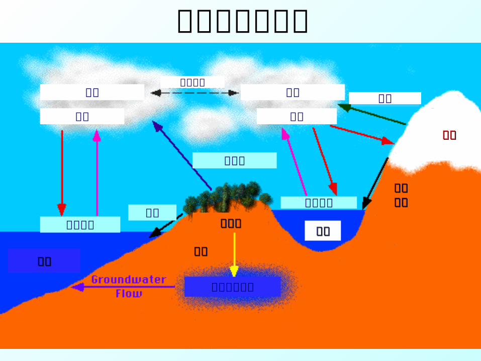
地下水含水层

融雪融雪径流径流

土壤水土壤水

下渗下渗湖泊湖泊

冰雪冰雪

海洋海洋

海洋蒸发

蒸散发

水面蒸发径流

降水 降水

水平对流凝结 凝结 升华

全球水循环框架

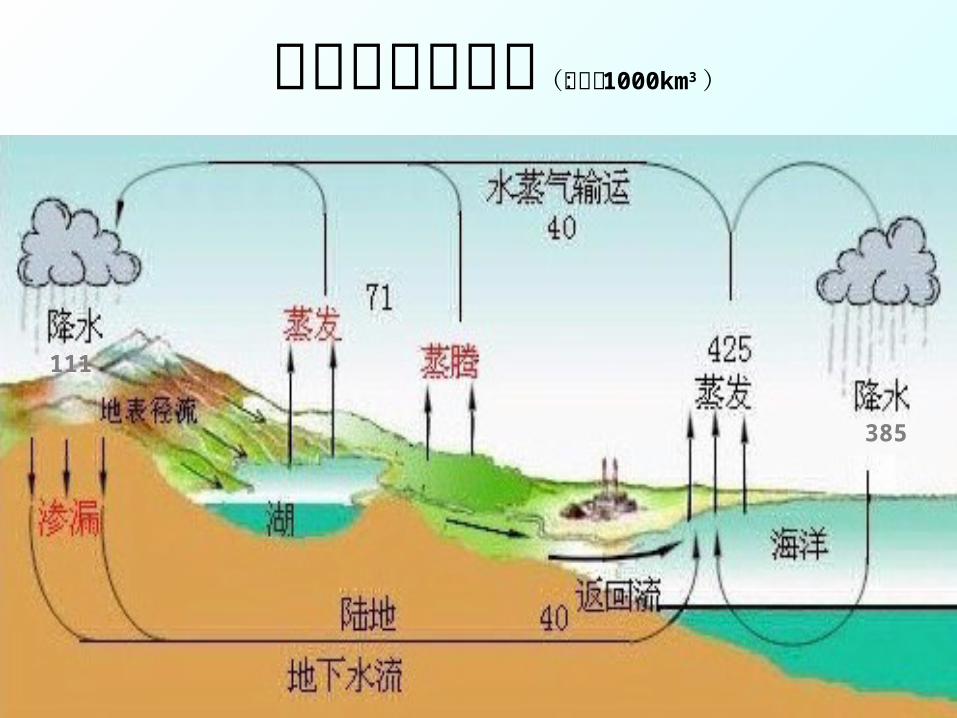
111

385

全球水循环数量（单位： 1000km3 ）

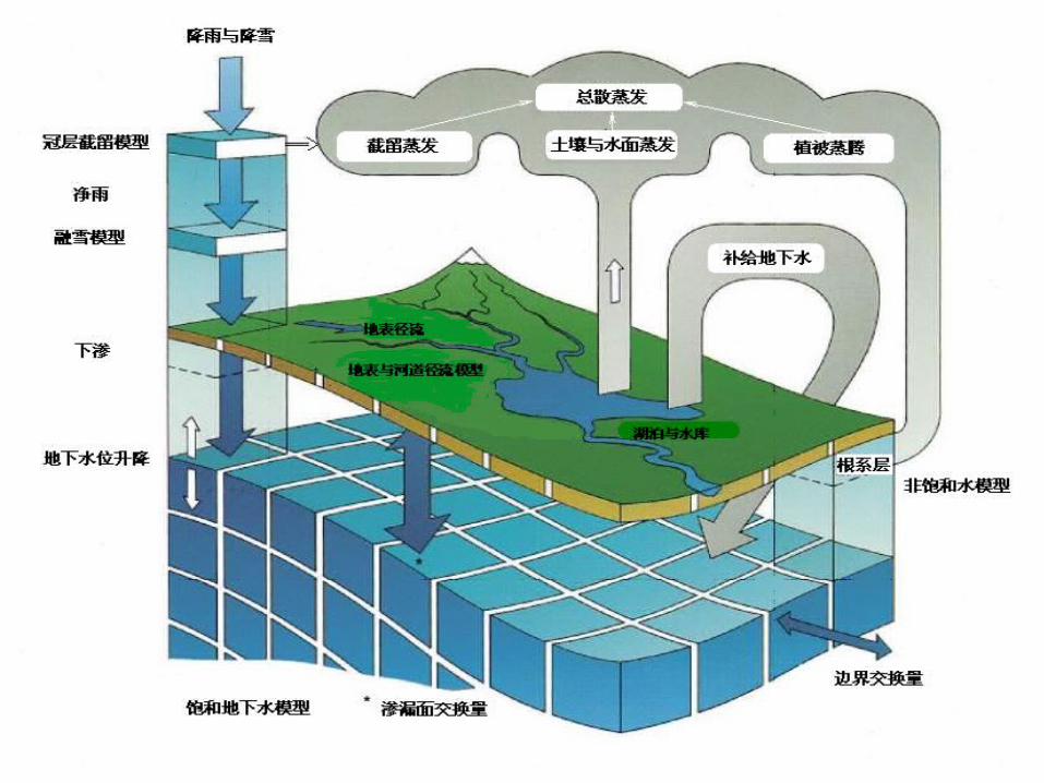
陆面过程 陆面过程是能够影响气候变化的发生在陆地表面土壤中控制陆地与大气之间动量、热量、及水分交换的那些过程；

• 陆面过程的简单介绍；陆面过程的简单介绍；• 陆面模式研究前沿问题；陆面模式研究前沿问题；• 在陆面模型及气候模拟中引入地下水位的动在陆面模型及气候模拟中引入地下水位的动 态变化的重要性；态变化的重要性；• 地下水位动态表示模型；地下水位动态表示模型；• 地表径流机制；地表径流机制；• 地下基流机制；地下基流机制；• 模型耦合及模拟模型耦合及模拟• 结论与讨论结论与讨论

陆面过程• 陆面过程是能够影响气候变化的发生在陆地表面土壤中控制陆地与大气之间动量、热量、及水分交换的那些过程；

• 这些过程受大气环流和气候的影响，反过来影响大气的运动，有不同的时空变化，由于人类活动改变地表的特性，使这些过程更为复杂；•如何准确描述气候模式中的大尺度陆面水文过程, 已经引起气候模式研究人员、水文学家和生态学家的关注。

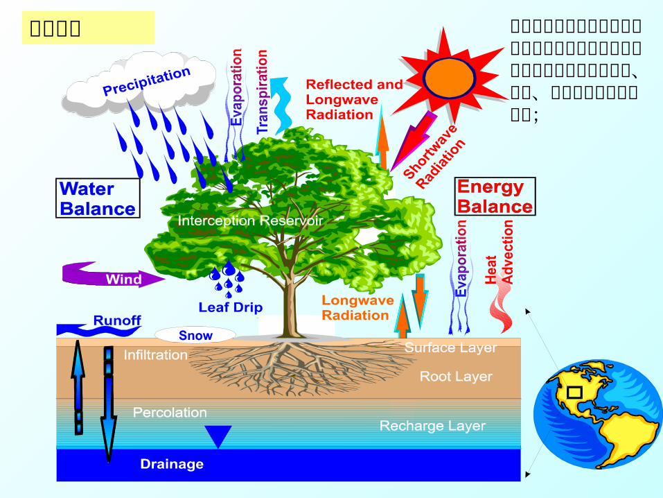
• 地面上的热力过程：发生在大气、植被和土壤表面的辐射过程（直接辐射、反射辐射和长波辐射）、土壤、植被、大气间的感热和潜热交换；

• 地面上的水文过程：大气降水、蒸发和植物蒸腾、凝结、地表径流以及冰雪融化和冻结；

• 地面上的动量交换：地面对风的摩擦和植被的阻挡；• 地表与大气的物质交换：气体、气溶胶、烟尘向上输送和大气悬垂物的沉落；

• 地面以下土壤的热传导与气隙中的热输送；• 地下的水文过程：大气降水、地面水的渗漏和深层水的上吸、植物根系的吸收、地下水流及土壤冻结和融化。

陆面过程的主要方面

陆面模式的发展经历了三代• 第一代从 60 年代末到 70 年代，用空气动力学总体输送

公式和几个均匀的陆地表面参数简单地参数化土壤水的蒸发和地表径流，即水桶模式（ Bucket ）；

• 第二代， 80 年代以来， GCM 中陆面参数化的一大进展是引入了植被生物物理过程，一系列不同详尽程度的陆面过程模式不断涌现，在本质上它们都属于计算土壤、植被与大气间交换方案（ SVATS ）；

• 第三代从 90 年代以后，植物生理学和生态学研究取得显著的进展以及卫星遥感技术的发展，考虑植物吸收 CO2 进行光合作用的生物化学模式引入陆面模式中，使植物能生长并响应气候的变化，即考虑碳循环作用的第三代陆面过程模式。

陆面过程模型中地下水位动态表示 :– Dai, Zeng, and Dickinson ， 1998, NCAR LSM, BATS, IAP94(Y

ongjiu Dai and Qingcun Zeng, 1997). CLM prototype, the initial CLM code.

– December 2001: to be released with the whole CCSM package officially.

– Liang and Xie (2001) developed a new parameterization to represent the Horton runoff mechanism in VIC-3L and combined it effectively with the original representation of the Dunne runoff mechanism(Xie et al., 2003).

– 谢正辉等 , 1998, 中国科学 .– Liang, Xie, Huang,, 2003, Groundwater model (method 1) ， Journal of

Geophysical Research. – Liang, Xie, 2003, Global Planetary Change.– Yang and Xie, 2003, Groundwater model (method 2) , Progress in Natu

ral Progress. – 谢正辉等 , 2004, 大气科学 .– Yeh et al 2005 JC,Maxwell et al 2005, JHM.– Tian and Xie, et al, 2006, Science in China.

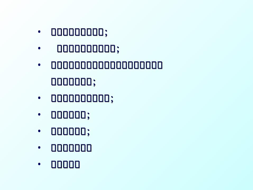
• 水文过程研究需要深入；• 生态过程机制（ C,N 循环）需要发展；• 各种非均匀性问题；• 雪盖、冻土和旱土、大面积水面作用的描述简单，冻土、雪盖占陆面面积都远大于 1/4 ，沙漠区占 1/4 ，水热耦合问题；

• 陆面模型参数移植与标定；• 陆面数据同化问题；• 与区域与全球气候模式的耦合；• 各种应用问题。

陆面模式研究前沿问题陆面模式研究前沿问题

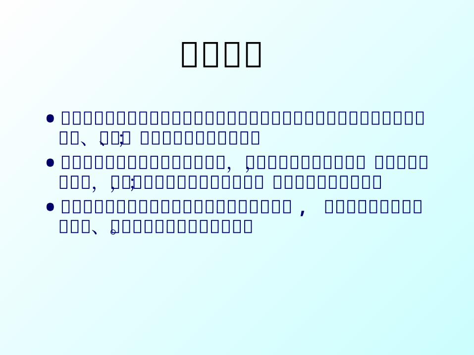
• 气候变化引起区域水文生态过程的变化

• 地表地下水文及陆地覆盖变化引起气候的改变• 气候与植被、地表水、地下水有重要的相互作用

土地沙化 生态环境恶化

北方干旱南方洪涝 高原冰川退化

河道干枯 地下水位下降植被减少

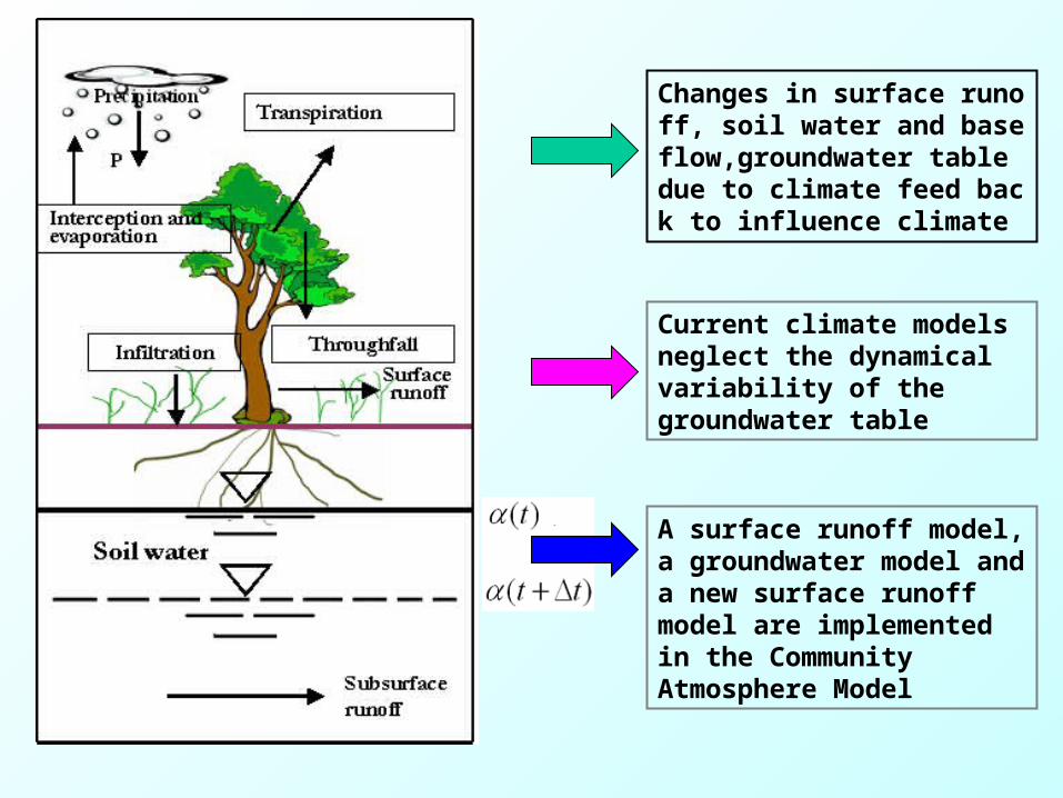
Changes in surface runoff, soil water and baseflow,groundwater table due to climate feed back to influence climate

Current climate models neglect the dynamical variability of the groundwater table

A surface runoff model, a groundwater model and a new surface runoff model are implemented in the Community Atmosphere Model

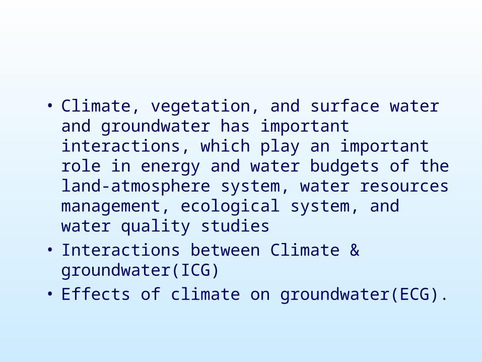
• Climate, vegetation, and surface water and groundwater has important interactions, which play an important role in energy and water budgets of the land-atmosphere system, water resources management, ecological system, and water quality studies

• Interactions between Climate & groundwater(ICG)• Effects of climate on groundwater(ECG).

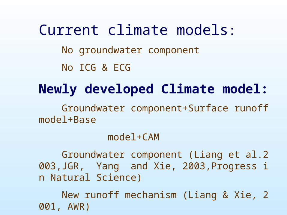
Current climate models:

No groundwater component

No ICG & ECG

Newly developed Climate model:

Groundwater component+Surface runoff model+Base

model+CAM

Groundwater component (Liang et al.2003,JGR, Yang and Xie, 2003,Progress in Natural Science)

New runoff mechanism (Liang & Xie, 2001, AWR)

Subsurface runoff (Tian and Xie, 2006, Science in China)

 

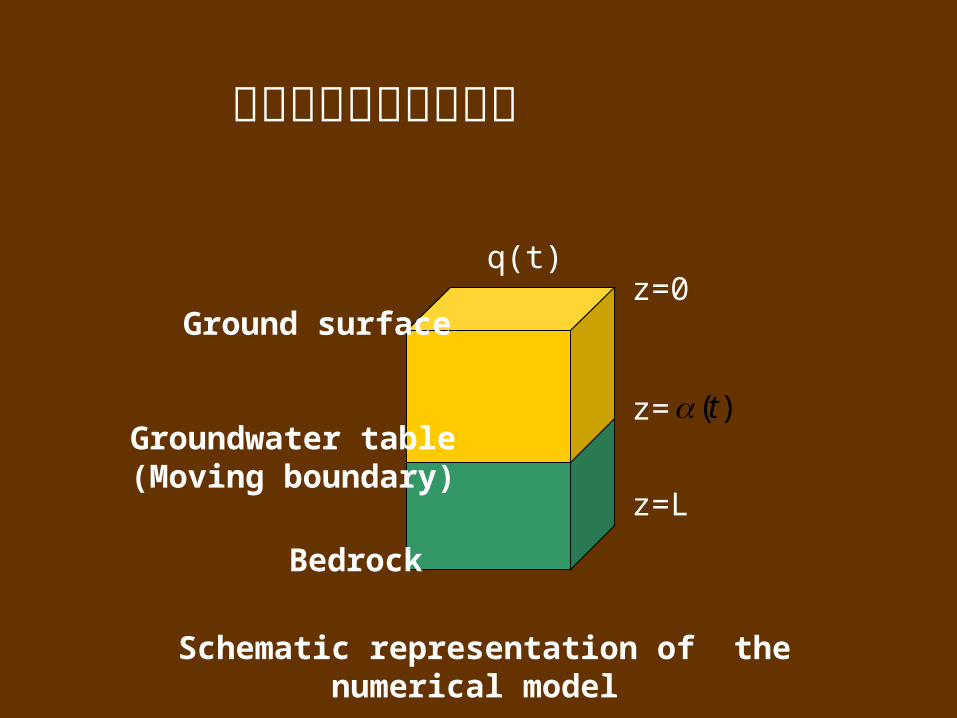
 z=

z=0

z=L 

Groundwater table(Moving boundary) 

Ground surface

Bedrock

q(t)

Schematic representation of the numerical model

)(t

地下水位动态表示模型

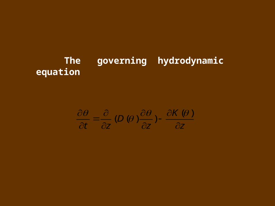
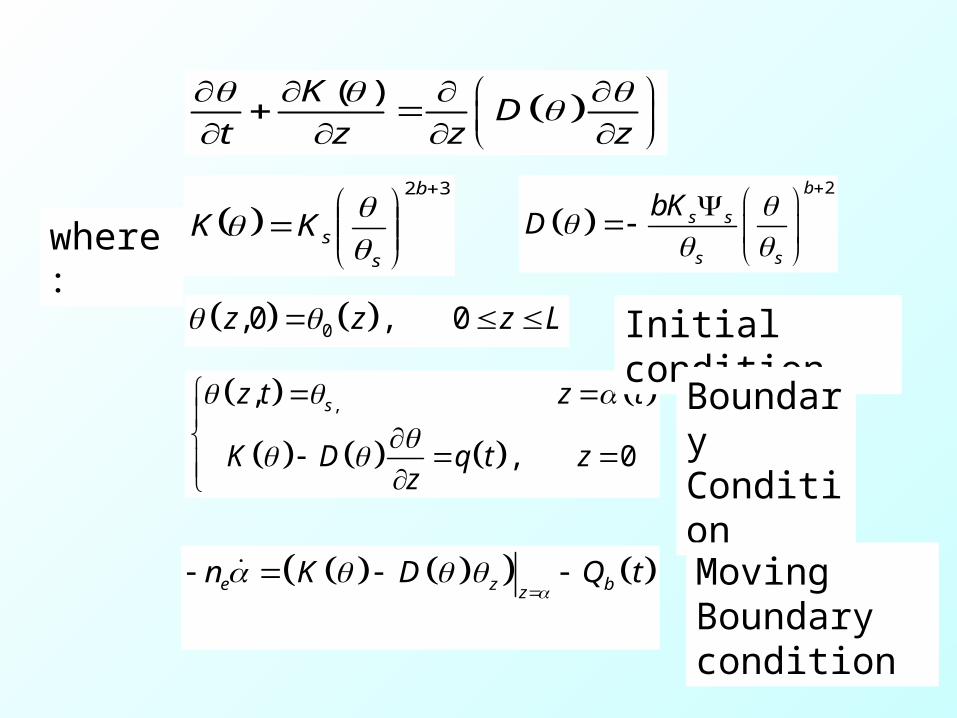
The governing hydrodynamic equation

( )( ( ) )

KD

t z z z

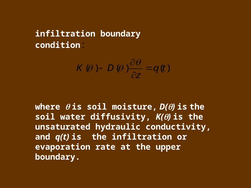
infiltration boundary condition:

)()()( tqz

DK

where is soil moisture, D() is the soil water diffusivity, K() is the unsaturated hydraulic conductivity, and q(t) is the infiltration or evaporation rate at the upper boundary.

where (t) is the ground table to the surface, and L is the depth from surface to the bedrock

Lzttz s )(,),(

For saturated zone:

( )KD

t z z z

0,0 , 0z z z L

,,

, 0

sz t z t

K D q t zz

Initial condition

Boundary Condition

32

b

ssKK

2b

s s

s s

bKD

where

：

e z bzn K D Q t

Moving

Boundary condition

( )KD

t z z z

,, sz t

K D q tz

e z bzn K D Q t

( )t 0,0z z

t

z

o

dt

dntQ

zDK ebtz

)()()()(

The moving boundary condition is

where ne is effective porosity.

The mass balance equation:

)0()()0,(),(1

)()(

0

)0(

0

)(

0

tt

es

dttqdzzdztzn

t

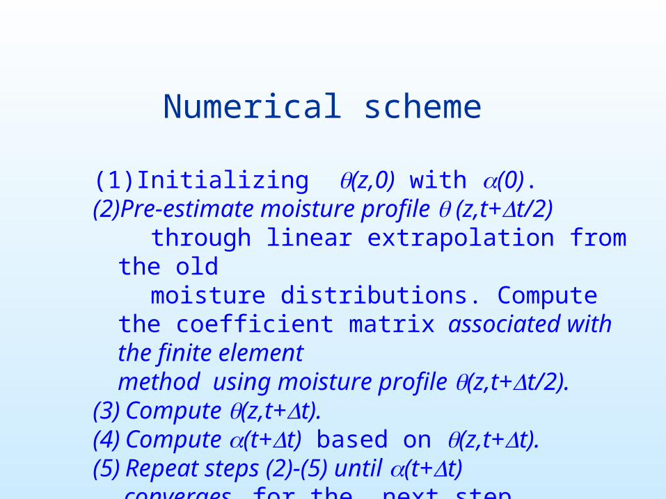
Numerical scheme

(1)Initializing (z,0) with (0).(2)Pre-estimate moisture profile (z,t+t/2) through linear extrapolation from the old moisture distributions. Compute the coefficient

matrix associated with the finite element method using moisture profile (z,t+t/2).(3)   Compute (z,t+t).(4)   Compute (t+t) based on (z,t+t).(5)   Repeat steps (2)-(5) until (t+t) converges for the next step.

Numerical schemesby two methods

• [0,L] is partitioned,moving boundary problem,Finite element, Mass lumped, direct method.

• [0, (t)], reducing the moving boundary problem into fixed boundary problem, Finite element, Mass lumped,

Indirect method.

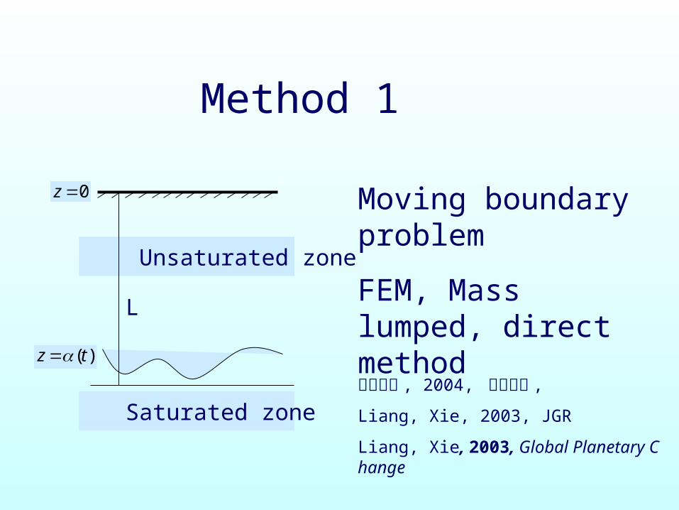
Unsaturated zone

Saturated zone

0z

( )z t

L

Moving boundary problem

FEM, Mass lumped, direct method

谢正辉等 , 2004, 大气科学 ,

Liang, Xie, 2003, JGR

Liang, Xie, 2003, Global Planetary Change

Method 1

• The following coordinate transformation is used

z

xt

t

Reduce a moving boundary problem into the fixed boundary problem

Method 2

Yang and Xie, 2003,

Progress in Natural Progress

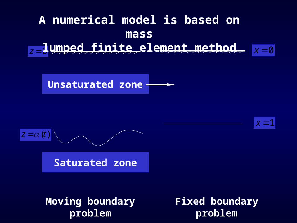
Unsaturated zone

Saturated zone

0z

( )z t

0x

1x

Moving boundary problem Fixed boundary problem

A numerical model is based on masslumped finite element method

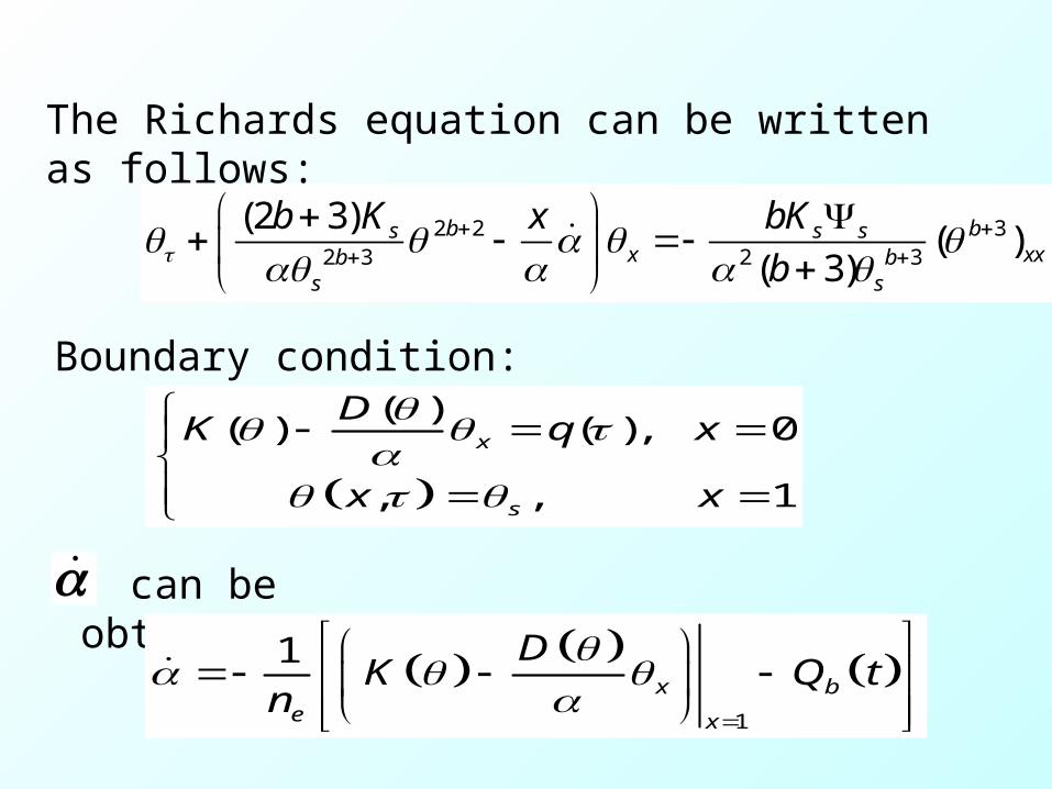
The Richards equation can be written as follows:

2 2 32 3 2 3

(2 3)( )

( 3)b bs s s

x xxb bs s

b K x bK

b

Boundary condition:

( )( ) ( ), 0

, , 1

x

s

DK q x

x x

can be obtained:

1

1x b

e x

DK Q t

n

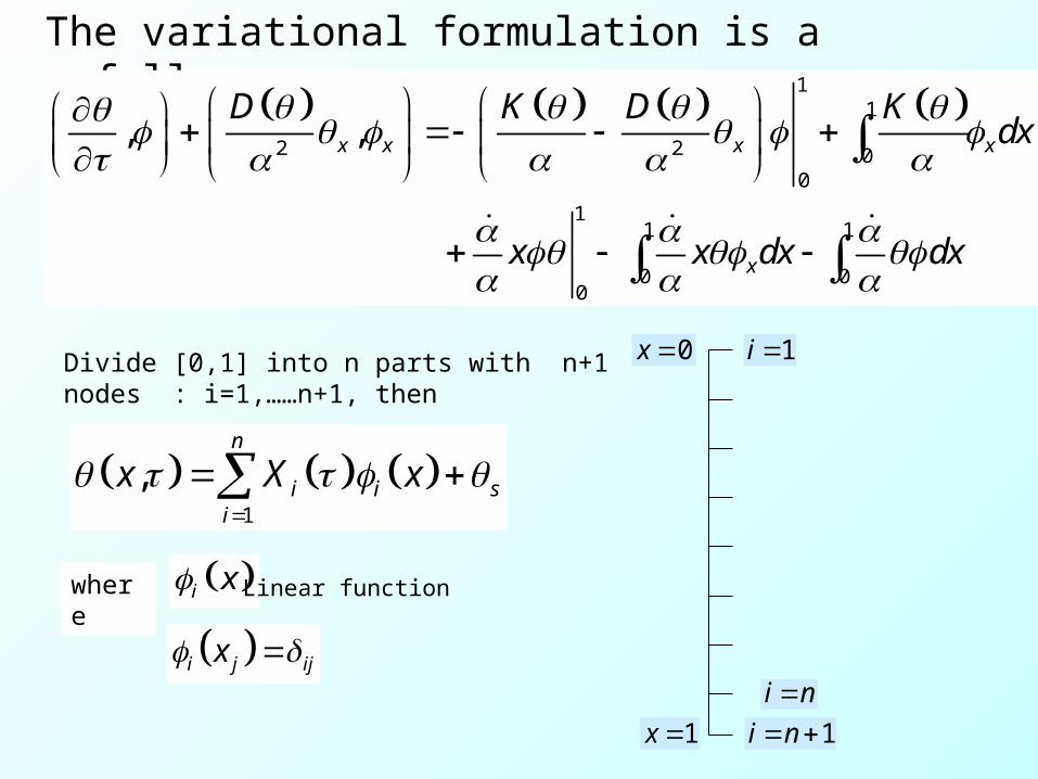
The variational formulation is as follows:

1

1

2 2 00

11 1

0 00

, ,x x x x

x

D K D Kdx

x x dx dx

Divide [0,1] into n parts with n+1 nodes : i=1,……n+1, then

1

,n

i i si

x X x

1i

1i n i n

0x

1x

where i x

i j ijx

Linear function

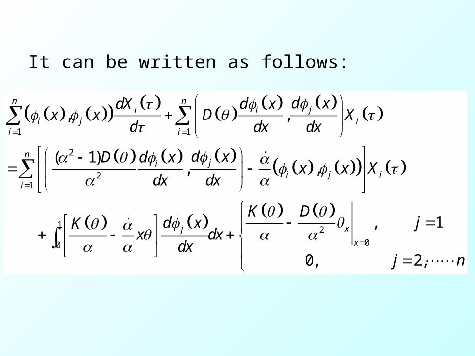
1 1

2

21

12

00

, ,

( 1), ,

, 1

0, 2,

n nji i

i j ii i

nji

i j ii

xj

x

d xdX d xx x D X

d dx dx

d xD d xx x X

dx dx

K Djd xK

x dxdx

j n

It can be written as follows:

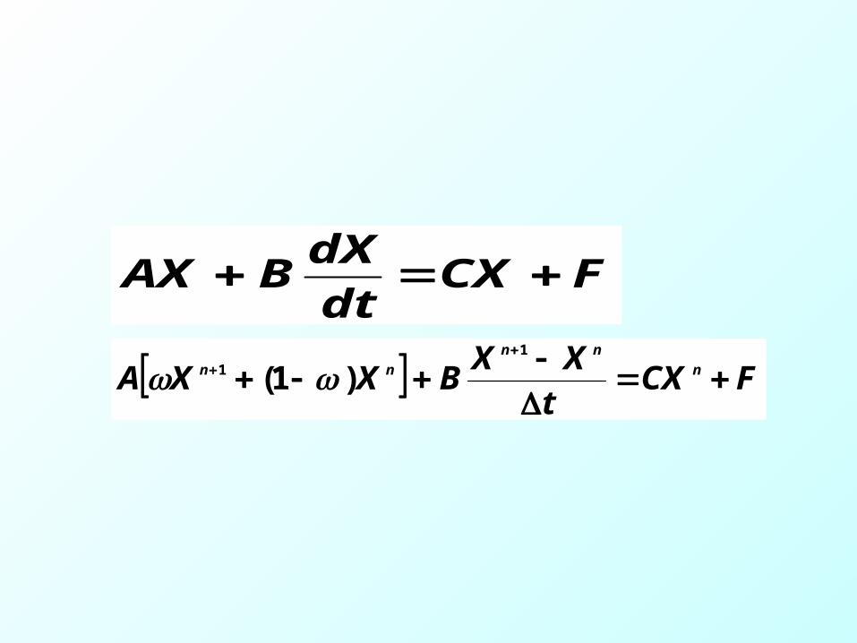
FCXdtdX

BAX

FCXt

XXBXXA n

nn

nn

1

1 )1(

同时考虑地下水位、潜水面水分通量与储存的地下径流机制

• 主要是以潜水面上的 Boussinesq 方程为基础来建立地下径流机制

• 在该方程线性化解析解的基础上，发展了同时考虑潜水面水分通量与储存量的地下径流机制

• 田向军 , 谢正辉 , 张生雷 , 梁妙龄，基于 Boussinesq-Storage同时考虑水分储存和入渗的地下径流机制，中国科学 (D), 2006

( )[cos ( ) sin ]

h k h h N th

t f x x x f

• The Dupuit-Boussinesq equation, describing the unconfined groundwater flow in a slope aquifer under a time-varying rate ,can be written as]/)[( TLtN

f

tN

x

h

x

hh

xf

k

t

h )(]sin)([cos

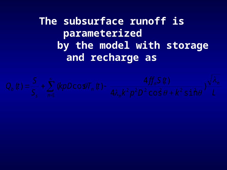
The subsurface runoff is parameterized by the model with storage and recharge

as

1222222

)sincos4

)(4)(cos()(

n

n

n

nn

sb LkDpk

tSfftTkpD

S

StQ

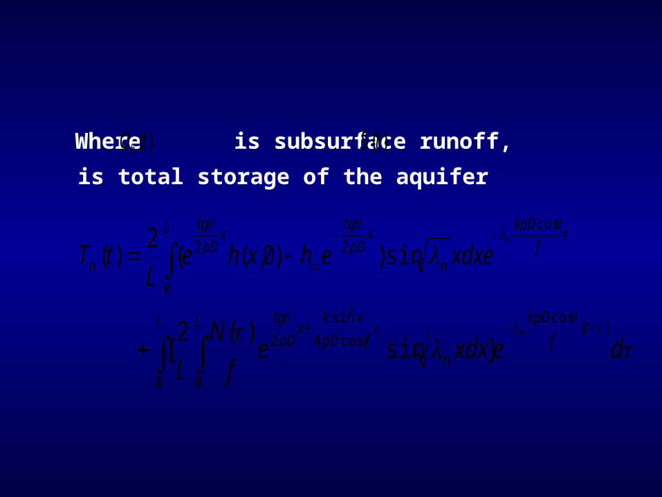
Where is subsurface runoff, is total storage of the

aquifer )(tQb )(tS

tf

kpD

n

L xpD

tgx

pD

tg

n

n

xdxeehxheL

tT

cos

0

22 sin))0,((2

)(

t t

f

kpDL

nfpD

xkx

pD

tg

dexdxef

N

L

n

0

)(cos

0

cos4

sin

2 ]sin)(2

[

2

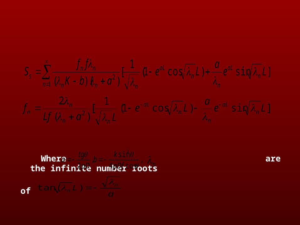
Where are the infinite number roots

of

1

2]sin)cos1(

1[

))((nn

aL

nn

aL

nnn

nns Le

aLe

abK

ffS

]sin)cos1(1

[)(

22

Lea

LeLaLf

f naL

nn

aL

nn

nn

,cos4

sin,

2

2

pDf

kb

pD

tga

n

aL n

n

)tan(

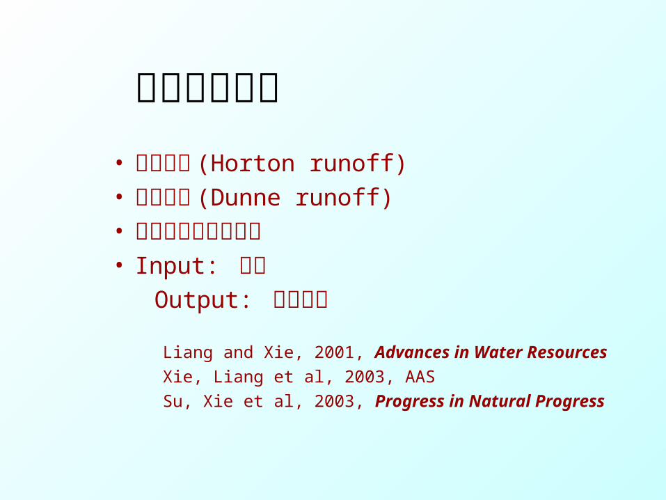
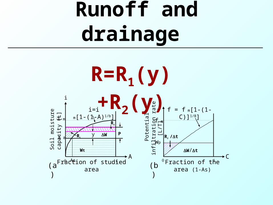
地表径流模型• 超渗产流 (Horton runoff) • 蓄满产流 (Dunne runoff)• 土壤次网格空间变率• Input: 降水 Output: 地表径流

Liang and Xie, 2001, Advances in Water Resources

Xie, Liang et al, 2003, AAS

Su, Xie et al, 2003, Progress in Natural Progress

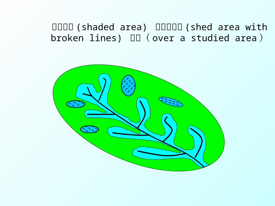
蓄满产流 (shaded area) 和超渗产流 (shed area with broken lines) 图表（ over a studied area ）

WR1

Fraction of studied area

Soi

l moi

stur

e ca

paci

ty [

L]

i=i m[1-(1-A)1/b]i m

R2

y

Fraction of the area (1-As)

f = f m[1-(1-C)]1/B]f m

f

Pot

enti

al in

filt

rati

on r

ate

[L/T

]

PR2 /t

W/t

C

i

As

wp

Wt

A

i 0

(a) (b)

Runoff and drainage

R=R1(y)+R2(y)

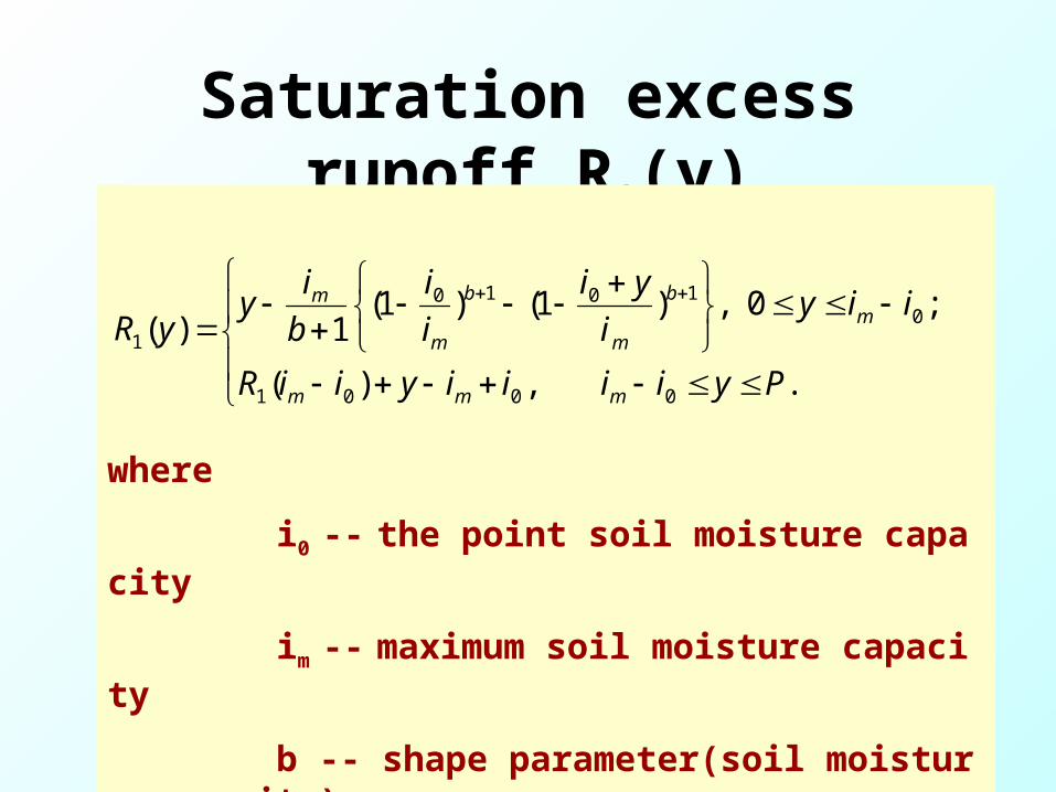
Saturation excess runoff R1(y)

where

i0 -- the point soil moisture capacity

im -- maximum soil moisture capacity

b -- shape parameter(soil moisture capacity)

P --precipitation

.,)(

;0,)1()1(1)(

0001

01010

1

PyiiiiyiiR

iiyi

yi

i

i

b

iy

yR

mmm

mb

m

b

m

m

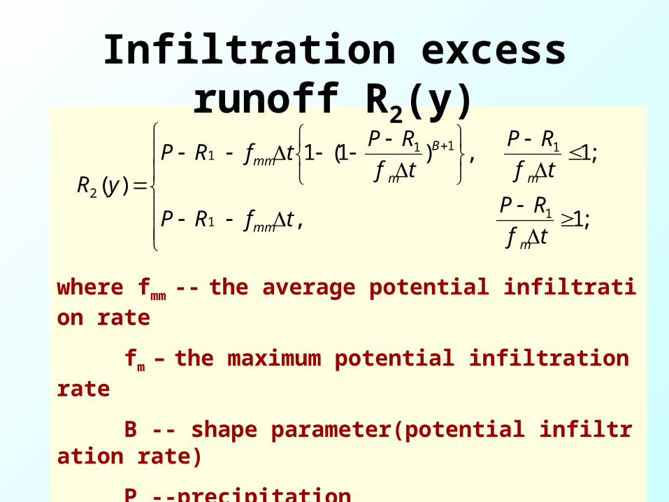
where fmm -- the average potential infiltration rate

fm – the maximum potential infiltration rate

B -- shape parameter(potential infiltration rate)

P --precipitation

∆t--time step

;1,

;1,)1(1

)(1

1

1111

2

tf

RPtfRP

tf

RP

tf

RPtfRP

yR

mmm

m

B

mmm

Infiltration excess runoff R2(y)

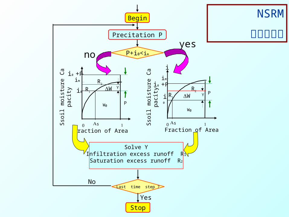
Precitation P

P+i0<im

W0

s Fraction of Area

Sso

il m

oist

ure

Cap

acit

y i0 +P

P

im

Solve YInfiltration excess runoff R1

Saturation excess runoff R2

W0

R1

s Fraction of Area

i0

P

im

R1Y

R2

Y

WW

Stop

Begin

yesno

i0 +Pi0

Last time step ?

Yes

No

ii

R2

NSRM

计算示意图

Sso

il m

oist

ure

Cap

acit

y

How to estimate fm

From

ΔW;0

t f Wf(t)dt0

We get tf, then fmm

);1)f(t(Bf

);f(tf

f

f

m

mm

•

Time (hour) Infi

ltra

tion

Rat

e (m

m/h

)

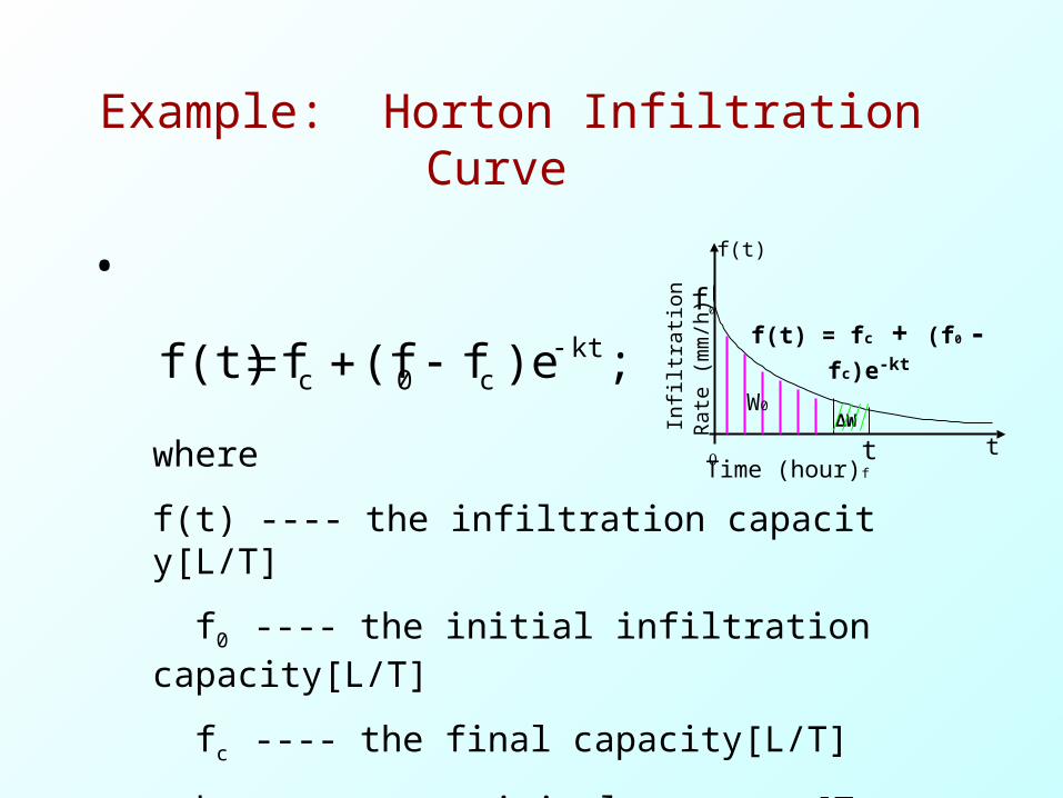
f(t) = fc + (f0 - fc)e-kt

f(t)

f0

ttf

W0ΔW

;)ef(fff(t) ktc0c

Example: Horton Infiltration Curve

where

f(t) ---- the infiltration capacity[L/T]

f0 ---- the initial infiltration capacity[L/T]

fc ---- the final capacity[L/T]

k ---- an empirical constant[T-1]

Time (hour) Infi

ltra

tion

Rat

e (m

m/h

)

f(t)

f0

ttf

W0ΔW

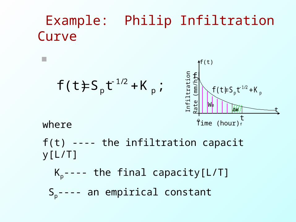
;KtSf(t) pp 2/1

Example: Philip Infiltration Curve

where

f(t) ---- the infiltration capacity[L/T]

Kp---- the final capacity[L/T]

Sp---- an empirical constant

pp KtSf(t) 2/1

CLM+ 地表径流 + 地下水 + 基流

1. Groundwater2. Runoff and subsurface para

meterization: the surface model ( 蓄满、超渗、土壤次网格课件变率 )

3. Subsurface parameterization ：同时考虑潜水面水分通量与储存量

Land framework

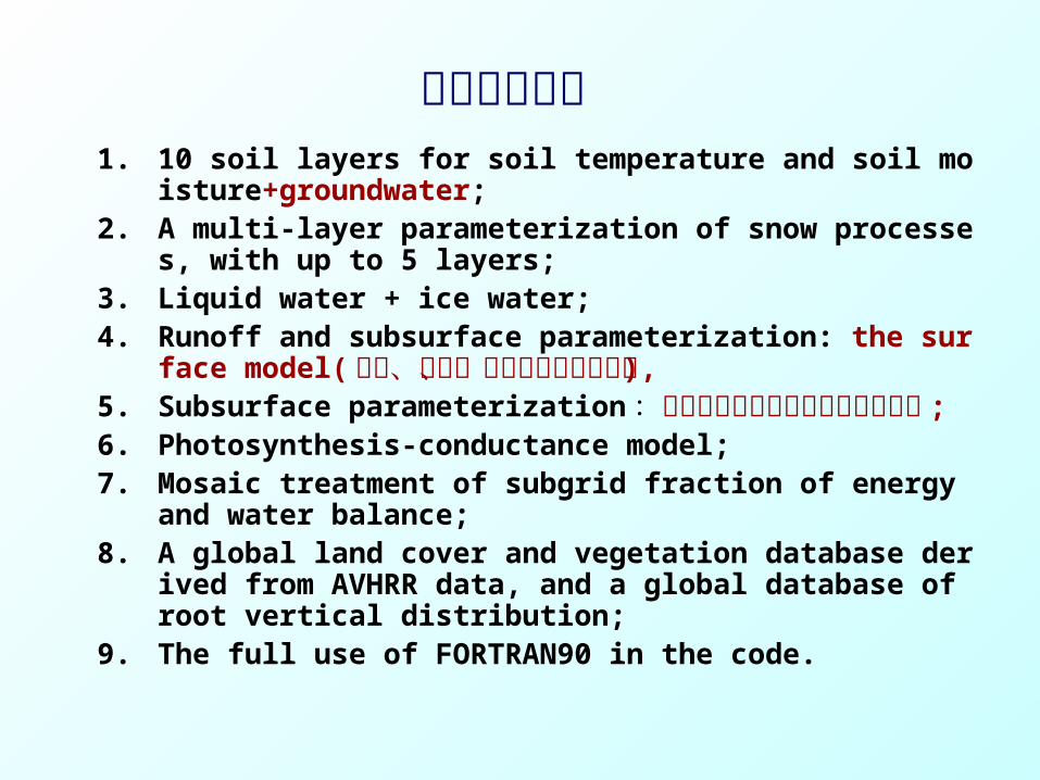
模型主要特征1. 10 soil layers for soil temperature and soil moisture+grou

ndwater;2. A multi-layer parameterization of snow processes, with u

p to 5 layers; 3. Liquid water + ice water;4. Runoff and subsurface parameterization: the surface mo

del( 蓄满、超渗、土壤次网格课件变率 ),5. Subsurface parameterization ：同时考虑潜水面水分通量与

储存量 ; 6. Photosynthesis-conductance model;7. Mosaic treatment of subgrid fraction of energy and water

balance; 8. A global land cover and vegetation database derived fro

m AVHRR data, and a global database of root vertical distribution;

9. The full use of FORTRAN90 in the code.

The new land surface model: CLM+NDMs

Remark: Land surface model+NDM

Coupling of CLM and NDMs

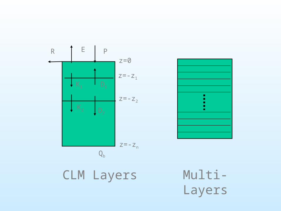
ER P

K2

K1

D2

D1

Qb

z=-zn

z=-z1

z=0

z=-z2

CLM Layers Multi-Layers

Comparison of daily observed groundwater table with the simulated groundwater table at the well Haizhou

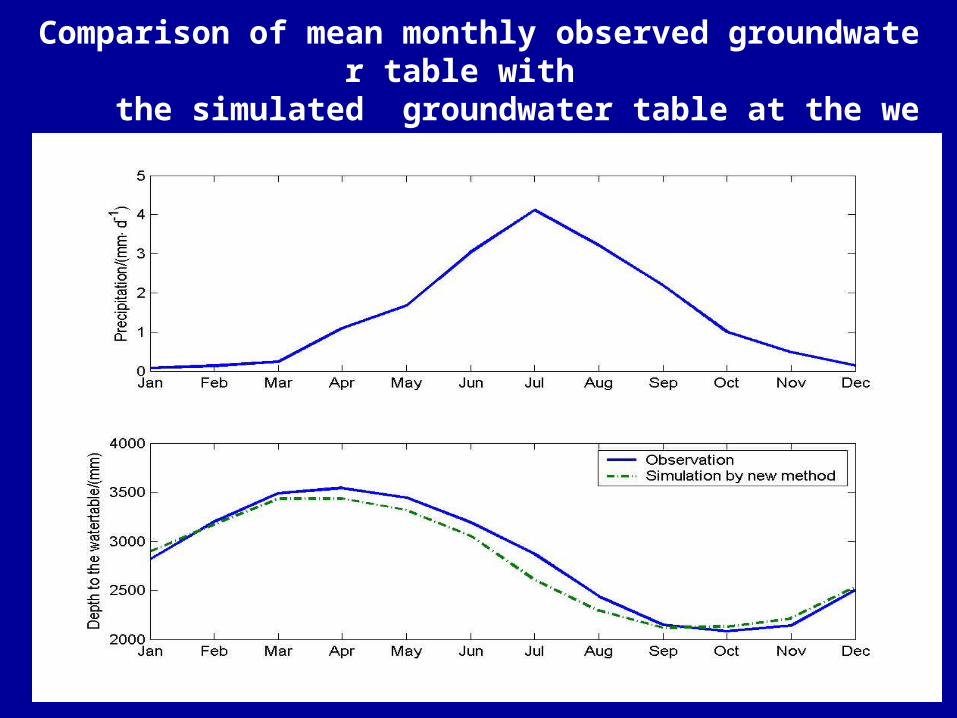
Comparison of mean monthly observed groundwater table with the simulated groundwater table at the well Haizhou

The new climate model: CAM+Groundwater component+Surface

runoff model+Base model

Coupling of the three hydrologicalmechanisms with the Climatemodel CAM

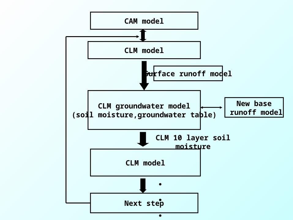
CLM groundwater model(soil moisture,groundwater table)

Surface runoff model

CLM model

Next step

CLM model

CAM model

New base runoff model

CLM 10 layer soil moisture

. . .

• Dynamic variation of groundwater table can be described as a moving boundary problem, which can be reduced to a fixed boundary problem through a coordinate transformation. With this method, the computational cost is decreased;

• The numerical simulations by the newly developed groundwater model coupled with CLM show that the land surface model can simulate dynamic variation of groundwater table;

• It has potential to explore interactions between land and atmosphere.

谢谢各位！ zxie@lasg.iap.ac.cn

Thank You for your attention!