Topic Model（≈

𝟏

𝟐Text Mining）

Yueshen Xuxyshzjucs@zju.edu.cn

Middleware, CCNT, ZJU

Middleware, CCNT, ZJU6/11/2014

Text Mining&NLP&ML

1, Yueshen Xu

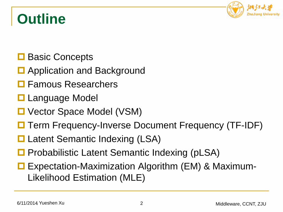
Outline

Basic Concepts

Application and Background

Famous Researchers

Language Model

Vector Space Model (VSM)

Term Frequency-Inverse Document Frequency (TF-IDF)

Latent Semantic Indexing (LSA)

Probabilistic Latent Semantic Indexing (pLSA)

Expectation-Maximization Algorithm (EM) & Maximum-

Likelihood Estimation (MLE)

6/11/2014 2 Middleware, CCNT, ZJU, Yueshen Xu

Outline

Latent Dirichlet Allocation (LDA)

Conjugate Prior

Possion Distribution

Variational Distribution and Variational Inference (VD

&VI)

Markov Chain Monte Carlo (MCMC)

Metropolis-Hastings Sampling (MH)

Gibbs Sampling and GS for LDA

Bayesian Theory v.s. Probability Theory

6/11/2014 3 Middleware, CCNT, ZJU, Yueshen Xu

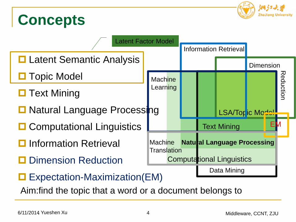
Concepts

Latent Semantic Analysis

Topic Model

Text Mining

Natural Language Processing

Computational Linguistics

Information Retrieval

Dimension Reduction

Expectation-Maximization(EM)

6/11/2014 Middleware, CCNT, ZJU

Information Retrieval

Computational Linguistics

Natural Language Processing

LSA/Topic Model

Text Mining

LSA/Topic Model

Data Mining

Reductio

n

Dimension

Machine

Learning

EM

4

Machine

Translation

Aim:find the topic that a word or a document belongs to

Latent Factor Model

, Yueshen Xu

Application

LFM has been a fundamental technique in modern

search engine, recommender system, tag extraction,

blog clustering, twitter topic mining, news (text)

summarization, etc.

Search Engine PageRank How important….this web page?

LFM How relevance….this web page?

LFM How relevance…the user’s query

vs. one document?

Recommender System Opinion Extraction

Spam Detection

Tag Extraction

6/11/2014 5 Middleware, CCNT, ZJU

Text Summarization

Abstract Generation

Twitter Topic Mining

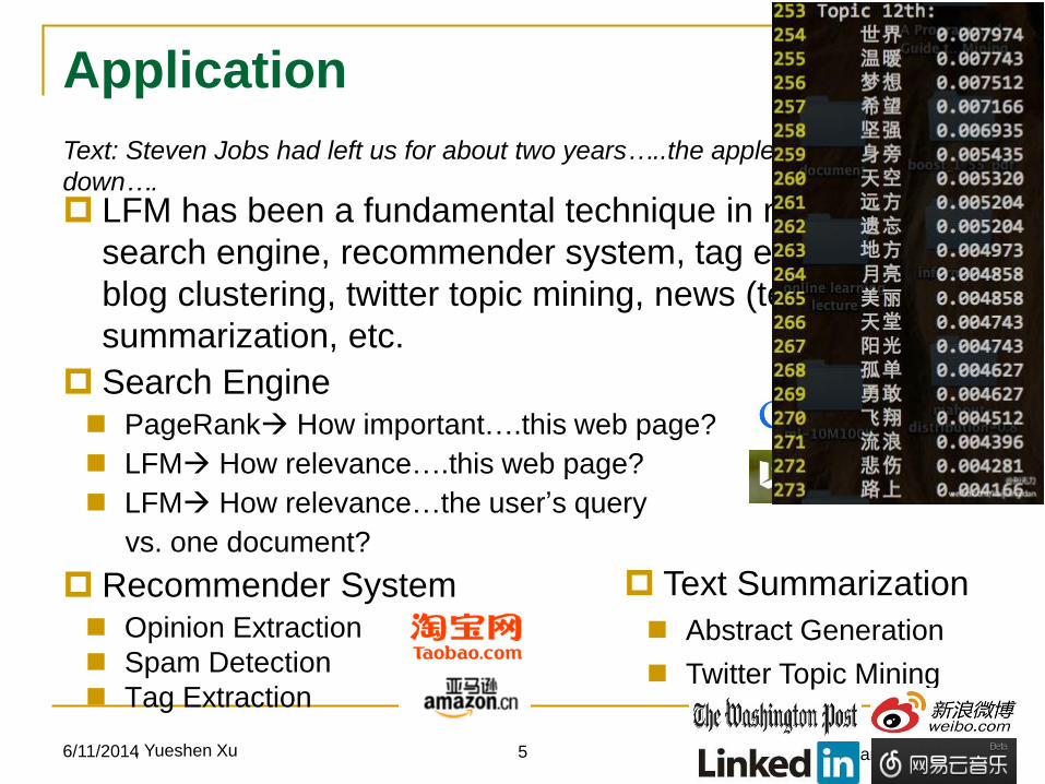
Text: Steven Jobs had left us for about two years…..the apple’s price will fall

down….

, Yueshen Xu

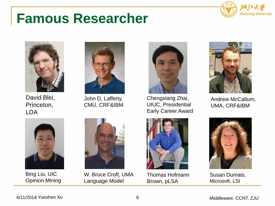
Famous Researcher

6/11/2014 6 Middleware, CCNT, ZJU

David Blei,

Princeton,

LDA

Chengxiang Zhai,

UIUC, Presidential

Early Career Award

W. Bruce Croft, UMA

Language Model

Bing Liu, UIC

Opinion Mining

John D. Lafferty,

CMU, CRF&IBM

Thomas Hofmann

Brown, pLSA

Andrew McCallum,

UMA, CRF&IBM

Susan Dumais,

Microsoft, LSI

, Yueshen Xu

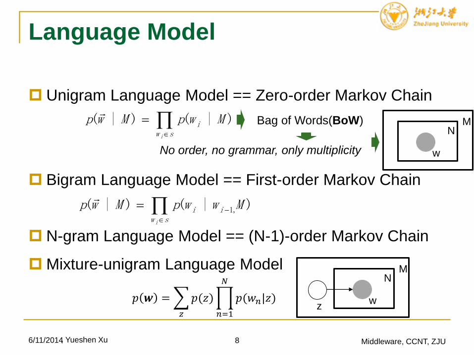
Language Model

Unigram Language Model == Zero-order Markov Chain

Bigram Language Model == First-order Markov Chain

N-gram Language Model == (N-1)-order Markov Chain

Mixture-unigram Language Model

6/11/2014 Middleware, CCNT, ZJU

sw

i

i

MwpMwp )|()|(

Bag of Words(BoW)

No order, no grammar, only multiplicity

sw

ii

i

MwwpMwp )|()|( ,1

8

w

NM

w

NM

z𝑝 𝒘 =

𝑧

𝑝(𝑧)

𝑛=1

𝑁

𝑝(𝑤𝑛|𝑧)

, Yueshen Xu

9

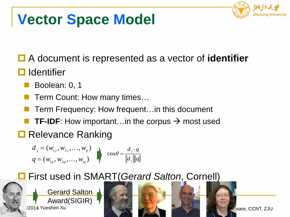
Vector Space Model

A document is represented as a vector of identifier

Identifier

Boolean: 0, 1

Term Count: How many times…

Term Frequency: How frequent…in this document

TF-IDF: How important…in the corpus most used

Relevance Ranking

First used in SMART(Gerard Salton, Cornell)

6/11/2014 Middleware, CCNT, ZJU

),,,(

),,,(

21

21

tqqq

tjjjj

wwwq

wwwd

Gerard Salton

Award(SIGIR)

qd

qd

j

j

cos

, Yueshen Xu

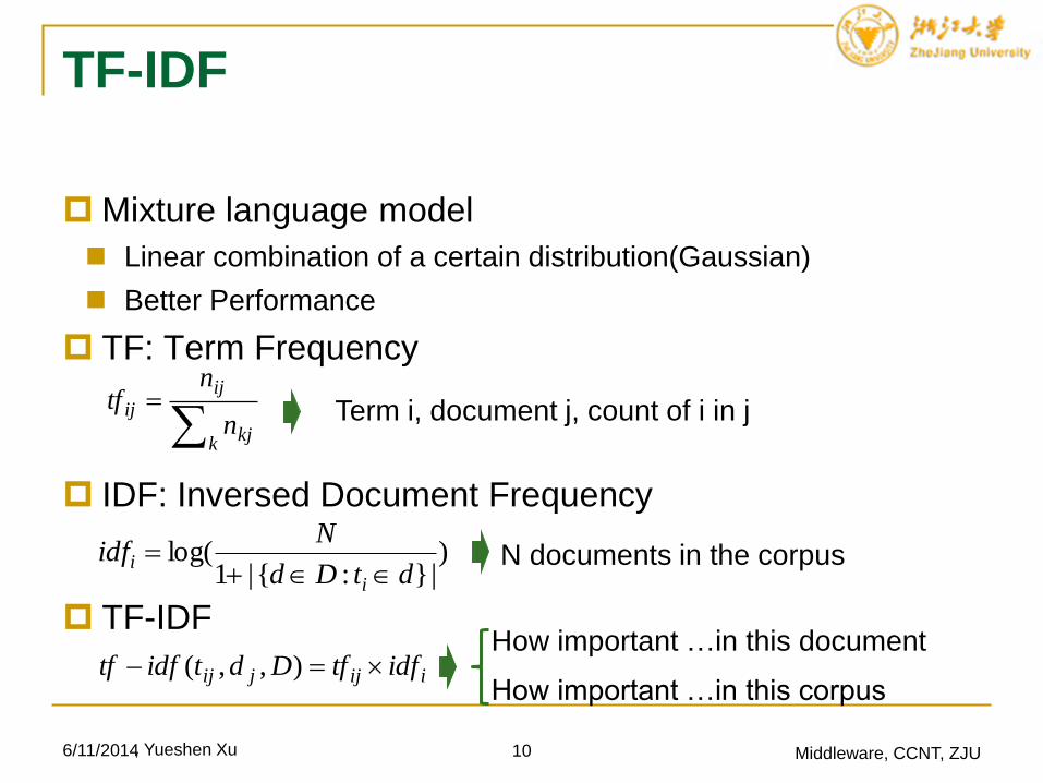
TF-IDF

Mixture language model

Linear combination of a certain distribution(Gaussian)

Better Performance

TF: Term Frequency

IDF: Inversed Document Frequency

TF-IDF

6/11/2014 Middleware, CCNT, ZJU

kkj

ij

ijn

ntf Term i, document j, count of i in j

)|}:{|1

log(dtDd

Nidf

i

i

N documents in the corpus

iijjij idftfDdtidftf ),,(How important …in this document

How important …in this corpus

10, Yueshen Xu

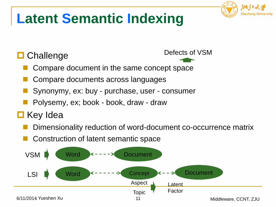
Latent Semantic Indexing

Challenge

Compare document in the same concept space

Compare documents across languages

Synonymy, ex: buy - purchase, user - consumer

Polysemy, ex; book - book, draw - draw

Key Idea

Dimensionality reduction of word-document co-occurrence matrix

Construction of latent semantic space

6/11/2014 Middleware, CCNT, ZJU

Defects of VSM

Word Document

Word DocumentConcept

VSM

LSI

11, Yueshen Xu

Aspect

Topic

Latent

Factor

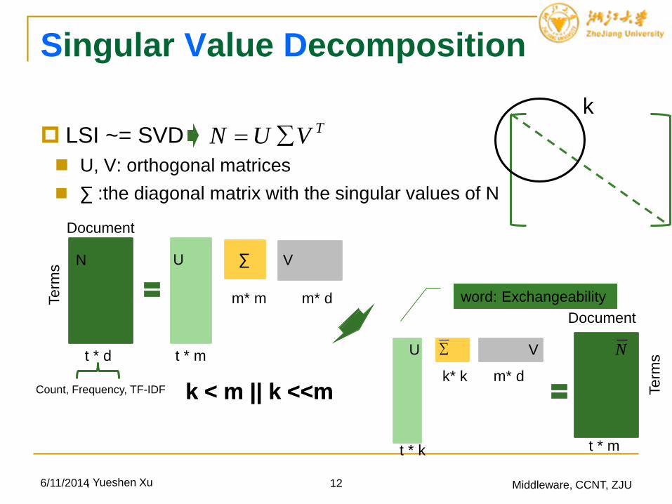
Singular Value Decomposition

LSI ~= SVD

U, V: orthogonal matrices

∑ :the diagonal matrix with the singular values of N

6/11/2014 Middleware, CCNT, ZJU12

TVUN

U

t * m

Document

Term

s

t * d

m* m m* d

N ∑U V

k < m || k <<mCount, Frequency, TF-IDF

t * m

Document

Term

s

t * k

k* k m* d

U V N

word: Exchangeability

k < m || k <<m

k

, Yueshen Xu

Singular Value Decomposition

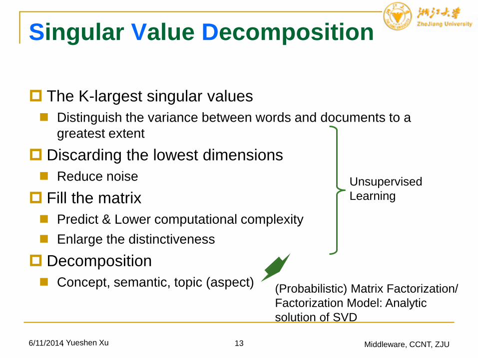
The K-largest singular values

Distinguish the variance between words and documents to a

greatest extent

Discarding the lowest dimensions

Reduce noise

Fill the matrix

Predict & Lower computational complexity

Enlarge the distinctiveness

Decomposition

Concept, semantic, topic (aspect)

6/11/2014 13 Middleware, CCNT, ZJU

(Probabilistic) Matrix Factorization/

Factorization Model: Analytic

solution of SVD

Unsupervised

Learning

, Yueshen Xu

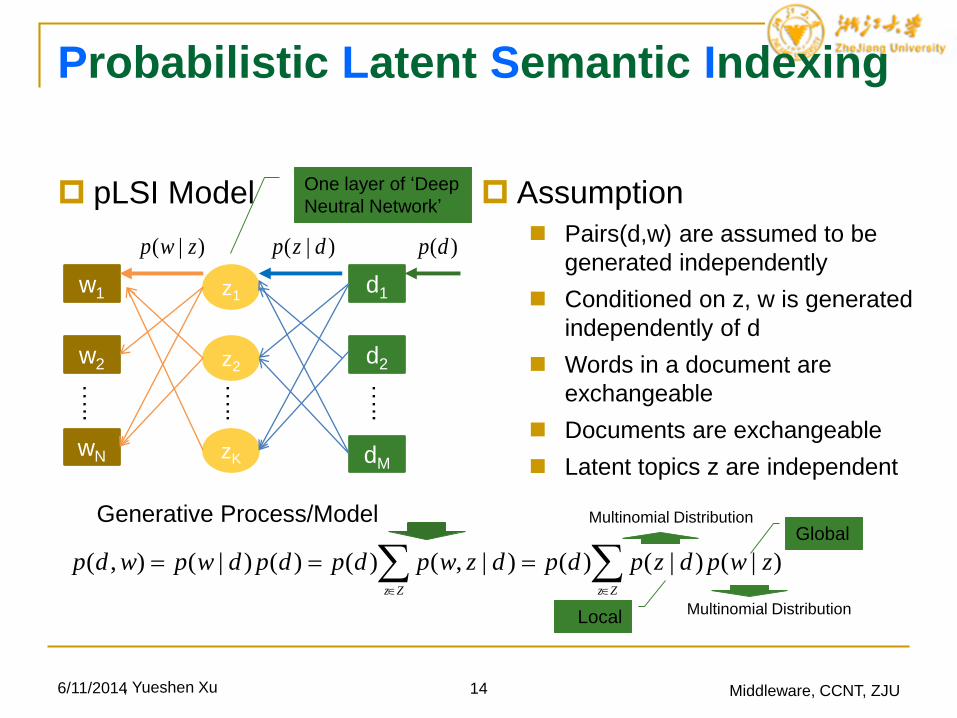
Probabilistic Latent Semantic Indexing

pLSI Model

6/11/2014 14 Middleware, CCNT, ZJU

w1

w2

wN

z1

zK

z2

d1

d2

dM

…..

…..

…..

)(dp)|( dzp)|( zwp

Assumption

Pairs(d,w) are assumed to be

generated independently

Conditioned on z, w is generated

independently of d

Words in a document are

exchangeable

Documents are exchangeable

Latent topics z are independent

Generative Process/Model

ZzZz

zwpdzpdpdzwpdpdpdwpwdp )|()|()()|,()()()|(),(

Multinomial Distribution

Multinomial Distribution

One layer of ‘Deep

Neutral Network’

Global

Local

, Yueshen Xu

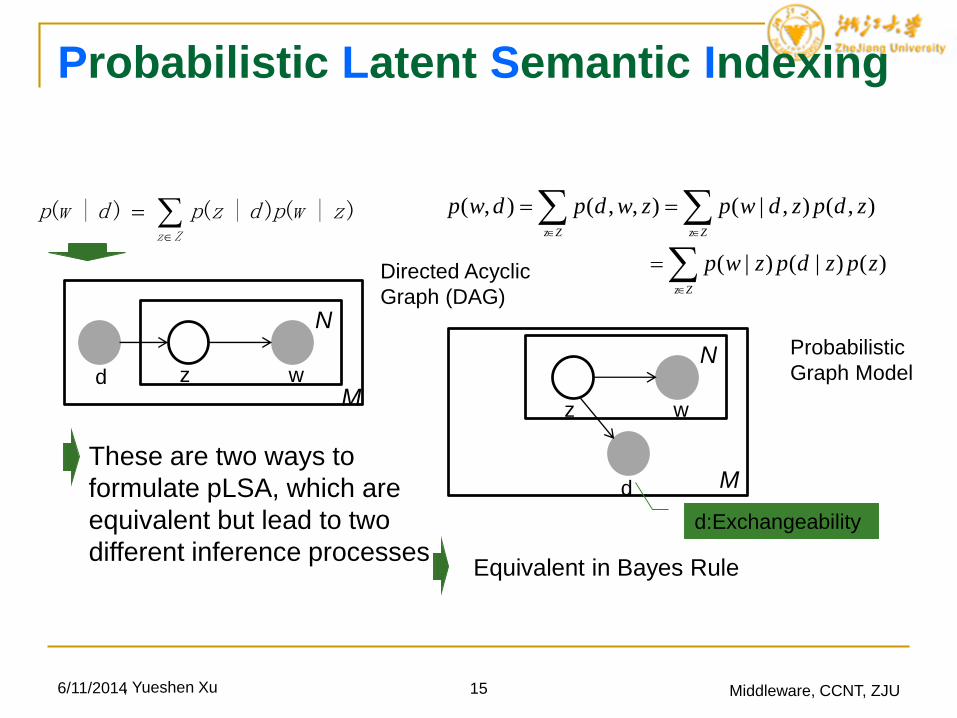
Probabilistic Latent Semantic Indexing

6/11/2014 15 Middleware, CCNT, ZJU

d z w

N

M

Zz

zwpdzpdwp )|()|()|(

Zz

ZzZz

zpzdpzwp

zdpzdwpzwdpdwp

)()|()|(

),(),|(),,(),(

d

z w

N

MThese are two ways to

formulate pLSA, which are

equivalent but lead to two

different inference processesEquivalent in Bayes Rule

Probabilistic

Graph Model

d:Exchangeability

Directed Acyclic

Graph (DAG)

, Yueshen Xu

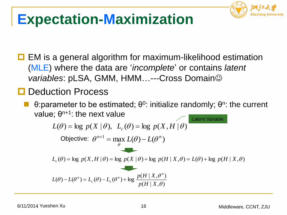
Expectation-Maximization

EM is a general algorithm for maximum-likelihood estimation

(MLE) where the data are ‘incomplete’ or contains latent

variables: pLSA, GMM, HMM…---Cross Domain

Deduction Process

θ:parameter to be estimated; θ0: initialize randomly; θn: the current

value; θn+1: the next value

6/11/2014 16 Middleware, CCNT, ZJU

)()(max1 nn LL

),|(log)( XpL )|,(log)( HXpLc Latent Variable

),|(log)(),|(log)|(log)|,(log)( XHpLXHpXpHXpLc

),|(

),|(log)()()()(

XHp

XHpLLLL

nn

cc

n

, Yueshen Xu

Objective:

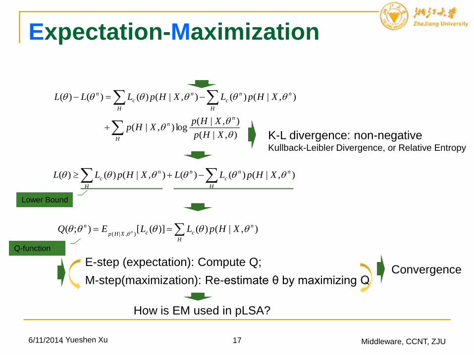
Expectation-Maximization

6/11/2014 17 Middleware, CCNT, ZJU

),|(

),|(log),|(

),|()(),|()()()(

XHp

XHpXHp

XHpLXHpLLL

n

H

n

H

nn

c

H

n

c

n

K-L divergence: non-negativeKullback-Leibler Divergence, or Relative Entropy

H

nn

c

H

nn

c XHpLLXHpLL ),|()()(),|()()(

Lower Bound

H

n

ccXHp

n XHpLLEQ n ),|()()]([);(),|(

Q-function

E-step (expectation): Compute Q;

M-step(maximization): Re-estimate θ by maximizing QConvergence

How is EM used in pLSA?

, Yueshen Xu

EM in pLSA

6/11/2014 18 Middleware, CCNT, ZJU

K

k

ikkjijk

N

i

M

j

ji

K

k

ikkj

N

i

M

j

jiijk

H

n

ccXHp

n

dzpzwpdwzpwdn

dzpzwpwdndwzp

XHpLLEQ n

11 1

1 1 1

),|(

))|()|(log(),|(),(

))|()|(log(),(),|(

),|()()]([);(

Posterior Random value in initialization

Likelyhood function

Constraints:

1.

2.

1)|(1

M

j

kjzwp

1)|(1

K

k

jkdzp

Lagrange

Multiplier

M

i

K

kiki

K

k

M

jkjkc dzpzwpLEH

1 11 1

))|(1())|(1(][

Partial derivative=0

independent

variable

independent

variable

M

m

N

i

imkim

N

i

ijkij

kj

dwzpdwn

dwzpdwn

zwp

1 1

1

),|(),(

),|(),(

)|()(

),|(),(

)|(1

i

M

j

ijkij

ikdn

dwzpdwn

dzp

M-Step

E-Step

K

l

illj

ikkj

K

l

illji

iikkj

ijk

dzpzwp

dzpzwp

dzpzwpdp

dpdzpzwpdwzp

1

1

)|()|(

)|()|(

)|()|()(

)()|()|(),|(

Associative

Law &

Distributive

Law

, Yueshen Xu

𝑙𝑜𝑔 𝑝(𝑤|𝑑)𝑛(𝑑,𝑤)

Bayesian Theory v.s.

Probability Theory

Bayesian Theory v.s. Probability Theory

Estimate 𝜃 through posterior v.s. Estimate 𝜃 through the

maximization of likelihood

Bayesian theory prior v.s. Probability theory statistic

When the number of samples → ∞, Bayesian theory == Probability

theory

Parameter Estimation

𝑝 𝜃 𝐷 ∝ 𝑝 𝐷 𝜃 𝑝 𝜃 𝑝 𝜃 ? Conjugate Prior likelihood is

helpful, but its function is limited Otherwise?

6/11/2014 19 Middleware, CCNT, ZJU

Non-parametric Bayesian Methods (Complicated)

Kernel methods: I just know a little...

VSM CF MF pLSA LDA Non-parametric Bayesian

Deep Learning

, Yueshen Xu

Latent Dirichlet Allocation

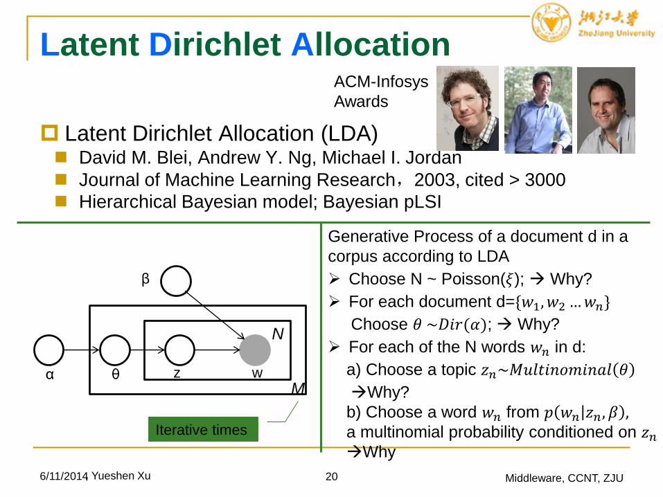
Latent Dirichlet Allocation (LDA) David M. Blei, Andrew Y. Ng, Michael I. Jordan

Journal of Machine Learning Research，2003, cited > 3000

Hierarchical Bayesian model; Bayesian pLSI

6/11/2014 20 Middleware, CCNT, ZJU

θ z w

N

Mα

β

Iterative times

Generative Process of a document d in a

corpus according to LDA

Choose N ~ Poisson(𝜉); Why?

For each document d={𝑤1, 𝑤2 … 𝑤𝑛}

Choose 𝜃 ~𝐷𝑖𝑟(𝛼); Why?

For each of the N words 𝑤𝑛 in d:

a) Choose a topic 𝑧𝑛~𝑀𝑢𝑙𝑡𝑖𝑛𝑜𝑚𝑖𝑛𝑎𝑙 𝜃

Why?

b) Choose a word 𝑤𝑛 from 𝑝 𝑤𝑛 𝑧𝑛, 𝛽 ,a multinomial probability conditioned on 𝑧𝑛

Why

ACM-Infosys

Awards

, Yueshen Xu

Latent Dirichlet Allocation

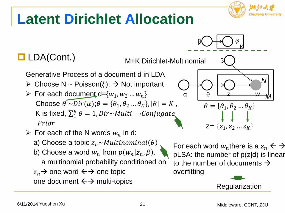
LDA(Cont.)

6/11/2014 21 Middleware, CCNT, ZJU

θ z w

N

Mα

𝜑

β

Kβ

Generative Process of a document d in LDA

Choose N ~ Poisson(𝜉); Not important

For each document d={𝑤1, 𝑤2 … 𝑤𝑛}

Choose 𝜃 ~𝐷𝑖𝑟(𝛼);𝜃 = 𝜃1, 𝜃2 … 𝜃𝐾 , 𝜃 = 𝐾 ,

K is fixed, 1𝐾 𝜃 = 1, 𝐷𝑖𝑟~𝑀𝑢𝑙𝑡𝑖 →𝐶𝑜𝑛𝑗𝑢𝑔𝑎𝑡𝑒

𝑃𝑟𝑖𝑜𝑟

For each of the N words 𝑤𝑛 in d:

a) Choose a topic 𝑧𝑛~𝑀𝑢𝑙𝑡𝑖𝑛𝑜𝑚𝑖𝑛𝑎𝑙 𝜃

b) Choose a word 𝑤𝑛 from 𝑝 𝑤𝑛 𝑧𝑛, 𝛽 ,

a multinomial probability conditioned on

𝑧𝑛 one word one topic

one document multi-topics

𝜃 = 𝜃1, 𝜃2 … 𝜃𝐾

z= 𝑧1, 𝑧2 … 𝑧𝐾

For each word 𝑤𝑛there is a 𝑧𝑛

pLSA: the number of p(z|d) is linear

to the number of documents

overfitting

Regularization

M+K Dirichlet-Multinomial

, Yueshen Xu

Latent Dirichlet Allocation

6/11/2014 22 Middleware, CCNT, ZJU, Yueshen Xu

Conjugate Prior &

Distributions

Conjugate Prior:

If the posterior p(θ|x) are in the same family as the p(θ), the prior

and posterior are called conjugate distributions, and the prior is

called a conjugate prior of the likelihood p(x|θ) : p(θ|x) ∝ p(x|θ)p(θ)

Distributions

Binomial Distribution ←→ Beta Distribution

Multinomial Distribution ←→ Dirichlet Distribution

Binomial & Beta Distribution

Binomial Bin(m|N,θ)=C(m,N)θm(1-θ)N-m :likelihood

C(m,N)=N!/(N-m)!m!

Beta(θ|a,b)

6/11/2014 23 Middleware, CCNT, ZJU

11- )1()()(

)(

ba

ba

ba

0

1)( dteta ta

Why do prior and

posterior need to be

conjugate distributions?

, Yueshen Xu

Conjugate Prior &

Distributions

6/11/2014 24 Middleware, CCNT, ZJU

11- )1()()(

)(

)1(),(),,,|(

ba

lm

ba

ba

lmmCbalmp

11- )1()()(

)(),,,|(

blam

blam

blambalmp

Beta Distribution!

Parameter Estimation

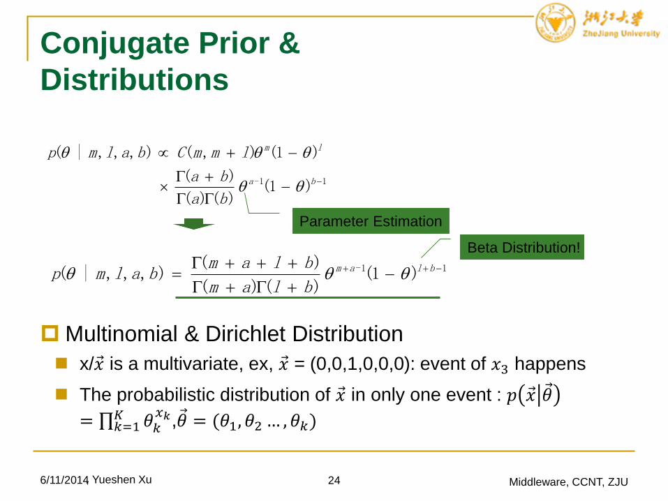
Multinomial & Dirichlet Distribution

x/ 𝑥 is a multivariate, ex, 𝑥 = (0,0,1,0,0,0): event of 𝑥3 happens

The probabilistic distribution of 𝑥 in only one event : 𝑝 𝑥 𝜃

= 𝑘=1𝐾 𝜃𝑘

𝑥𝑘, 𝜃 = (𝜃1, 𝜃2 … , 𝜃𝑘)

, Yueshen Xu

Conjugate Prior &

Distributions

Multinomial & Dirichlet Distribution (Cont.)

Mult(𝑚1, 𝑚2, … , 𝑚𝐾|𝜽, 𝑁)=𝑁!

𝑚1!𝑚2!…𝑚𝐾!𝐶𝑁

𝑚1𝐶𝑁−𝑚1

𝑚2 𝐶𝑁−𝑚1−𝑚2

𝑚3 …

𝐶𝑁− 𝑘=1

𝐾−1 𝑚𝑘

𝑚𝐾 𝑘=1𝐾 𝜃𝑘

𝑥𝑘: the likelihood function of 𝜃

6/11/2014 25 Middleware, CCNT, ZJU

Mult: The exact probabilistic distribution of 𝑝 𝑧𝑘 𝑑𝑗 and 𝑝 𝑤𝑗 𝑧𝑘

In Bayesian theory, we need to find a conjugate prior of 𝜃 for

Mult, where 0 < 𝜃 < 1, 𝑘=1𝐾 𝜃𝑘 = 1

Dirichlet Distribution

𝐷𝑖𝑟 𝜃 𝜶 =Γ(𝛼0)

Γ 𝛼1 … Γ 𝛼𝐾

𝑘=1

𝐾

𝜃𝑘𝛼𝑘−1

a vector

Hyper-parameter: parameter in

probabilistic distribution function (pdf), Yueshen Xu

Conjugate Prior &

Distributions

Multinomial & Dirichlet Distribution (Cont.)

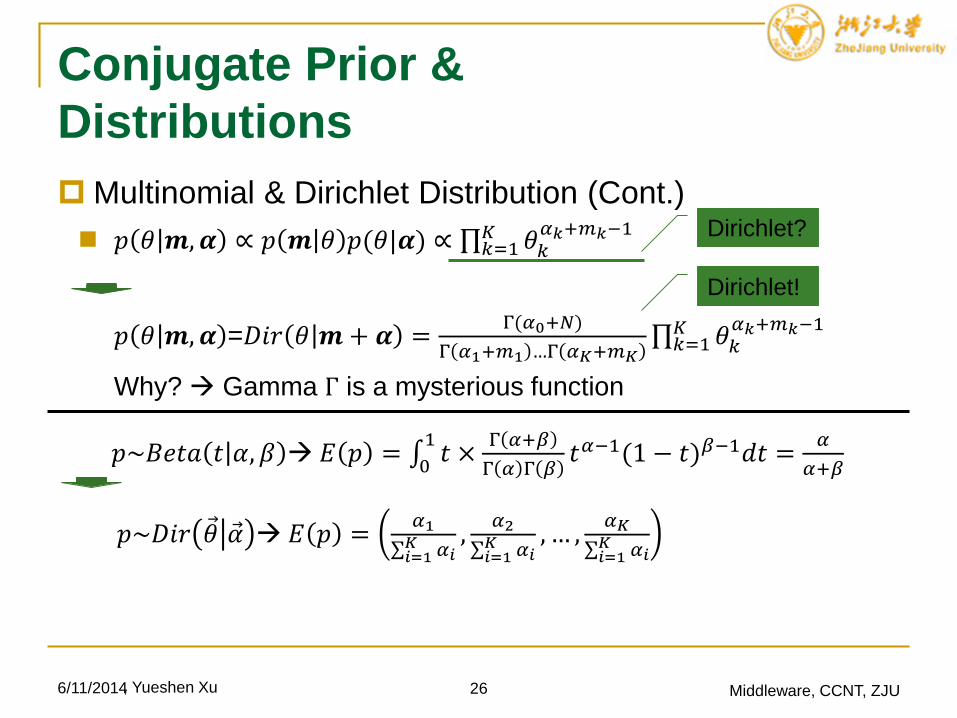
𝑝 𝜃 𝒎, 𝜶 ∝ 𝑝 𝒎 𝜃 𝑝(𝜃|𝜶) ∝ 𝑘=1𝐾 𝜃𝑘

𝛼𝑘+𝑚𝑘−1

6/11/2014 26 Middleware, CCNT, ZJU

Dirichlet?

𝑝 𝜃 𝒎, 𝜶 =𝐷𝑖𝑟 𝜃 𝒎 + 𝜶 =Γ(𝛼0+𝑁)

Γ 𝛼1+𝑚1 …Γ 𝛼𝐾+𝑚𝐾 𝑘=1

𝐾 𝜃𝑘𝛼𝑘+𝑚𝑘−1

Why? Gamma Γ is a mysterious function

Dirichlet!

𝑝~𝐵𝑒𝑡𝑎 𝑡 𝛼, 𝛽 𝐸 𝑝 = 0

1𝑡 ×

Γ 𝛼+𝛽

Γ 𝛼 Γ 𝛽𝑡𝛼−1(1 − 𝑡)𝛽−1𝑑𝑡 =

𝛼

𝛼+𝛽

𝑝~𝐷𝑖𝑟 𝜃 𝛼 𝐸 𝑝 =𝛼1

𝑖=1𝐾 𝛼𝑖

,𝛼2

𝑖=1𝐾 𝛼𝑖

, … ,𝛼𝐾

𝑖=1𝐾 𝛼𝑖

, Yueshen Xu

Poisson Distribution

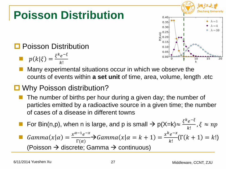
Why Poisson distribution?

The number of births per hour during a given day; the number of

particles emitted by a radioactive source in a given time; the number

of cases of a disease in different towns

For Bin(n,p), when n is large, and p is small p(X=k)≈𝜉𝑘𝑒−𝜉

𝑘!, 𝜉 ≈ 𝑛𝑝

𝐺𝑎𝑚𝑚𝑎 𝑥 𝛼 =𝑥𝛼−1𝑒−𝑥

Γ(𝛼)𝐺𝑎𝑚𝑚𝑎 𝑥 𝛼 = 𝑘 + 1 =

𝑥𝑘𝑒−𝑥

𝑘!(Γ 𝑘 + 1 = 𝑘!)

(Poisson discrete; Gamma continuous)

6/11/2014 27 Middleware, CCNT, ZJU

Poisson Distribution

𝑝 𝑘|𝜉 =𝜉𝑘𝑒−𝜉

𝑘!

Many experimental situations occur in which we observe the

counts of events within a set unit of time, area, volume, length .etc

, Yueshen Xu

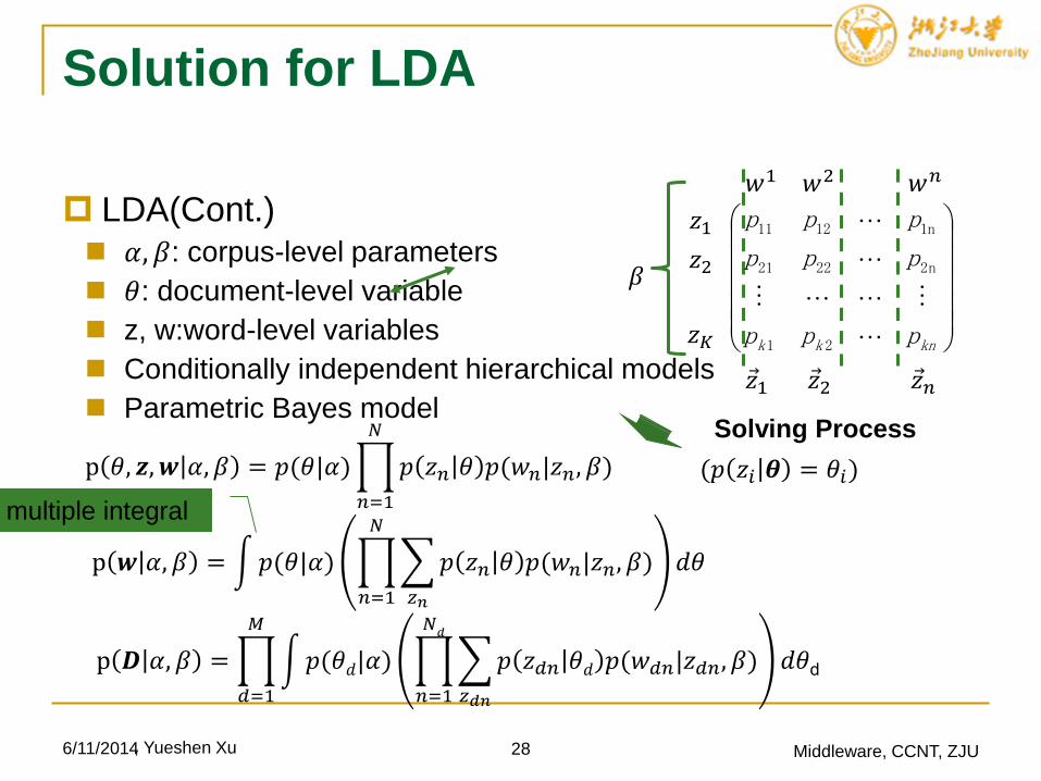
Solution for LDA

LDA(Cont.) 𝛼, 𝛽: corpus-level parameters

𝜃: document-level variable

z, w:word-level variables

Conditionally independent hierarchical models

Parametric Bayes model

6/11/2014 28 Middleware, CCNT, ZJU

knkk ppp

ppp

ppp

21

n22221

n11211𝑧1

𝑧2

𝑧𝐾

𝑤1

𝑧1 𝑧2 𝑧𝑛

𝑤2 𝑤𝑛

p 𝜃, 𝒛, 𝒘 𝛼, 𝛽 = 𝑝(𝜃|𝛼)

𝑛=1

𝑁

𝑝 𝑧𝑛 𝜃 𝑝(𝑤𝑛|𝑧𝑛, 𝛽)

Solving Process

(𝑝 𝑧𝑖 𝜽 = 𝜃𝑖)

p 𝒘 𝛼, 𝛽 = 𝑝(𝜃|𝛼)

𝑛=1

𝑁

𝑧𝑛

𝑝 𝑧𝑛 𝜃 𝑝(𝑤𝑛|𝑧𝑛, 𝛽) 𝑑𝜃

multiple integral

p 𝑫 𝛼, 𝛽 =

𝑑=1

𝑀

𝑝(𝜃𝑑|𝛼)

𝑛=1

𝑁𝑑

𝑧𝑑𝑛

𝑝 𝑧𝑑𝑛 𝜃𝑑 𝑝(𝑤𝑑𝑛|𝑧𝑑𝑛, 𝛽) 𝑑𝜃d

𝛽

, Yueshen Xu

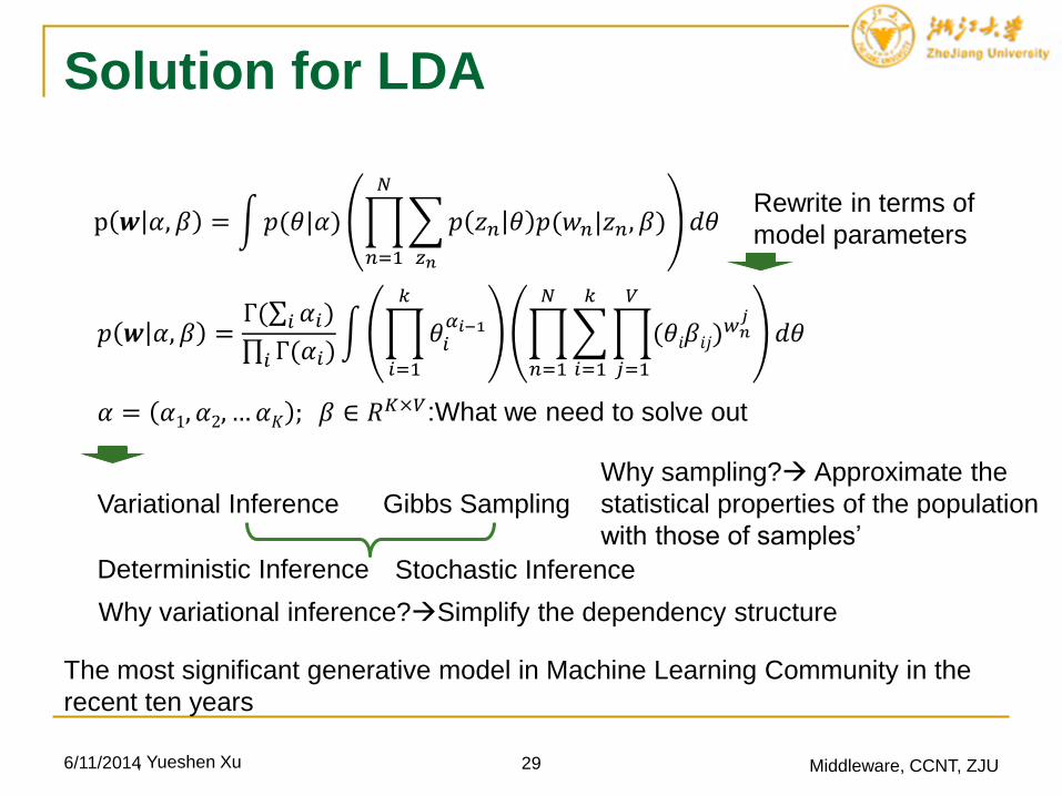
Solution for LDA

6/11/2014 29 Middleware, CCNT, ZJU

The most significant generative model in Machine Learning Community in the

recent ten years

𝑝 𝒘 𝛼, 𝛽 =Γ( 𝑖 𝛼𝑖)

𝑖 Γ(𝛼𝑖)

𝑖=1

𝑘

𝜃𝑖𝛼𝑖−1

𝑛=1

𝑁

𝑖=1

𝑘

𝑗=1

𝑉

(𝜃𝑖𝛽𝑖𝑗)𝑤𝑛

𝑗

𝑑𝜃

p 𝒘 𝛼, 𝛽 = 𝑝(𝜃|𝛼)

𝑛=1

𝑁

𝑧𝑛

𝑝 𝑧𝑛 𝜃 𝑝(𝑤𝑛|𝑧𝑛, 𝛽) 𝑑𝜃Rewrite in terms of

model parameters

𝛼 = 𝛼1, 𝛼2, … 𝛼𝐾 ; 𝛽 ∈ 𝑅𝐾×𝑉:What we need to solve out

Variational Inference Gibbs Sampling

Deterministic Inference Stochastic Inference

Why variational inference?Simplify the dependency structure

Why sampling? Approximate the

statistical properties of the population

with those of samples’

, Yueshen Xu

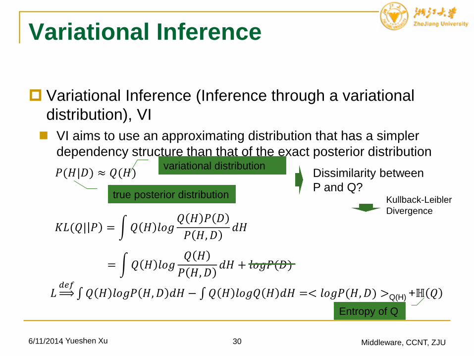
Variational Inference

Variational Inference (Inference through a variational

distribution), VI

VI aims to use an approximating distribution that has a simpler

dependency structure than that of the exact posterior distribution

6/11/2014 30 Middleware, CCNT, ZJU

𝑃(𝐻|𝐷) ≈ 𝑄(𝐻)

true posterior distribution

variational distributionDissimilarity between

P and Q?Kullback-Leibler

Divergence

𝐾𝐿(𝑄| 𝑃 = 𝑄 𝐻 𝑙𝑜𝑔𝑄 𝐻 𝑃 𝐷

𝑃 𝐻, 𝐷𝑑𝐻

= 𝑄 𝐻 𝑙𝑜𝑔𝑄 𝐻

𝑃 𝐻, 𝐷𝑑𝐻 + 𝑙𝑜𝑔𝑃(𝐷)

𝐿𝑑𝑒𝑓

𝑄 𝐻 𝑙𝑜𝑔𝑃 𝐻, 𝐷 𝑑𝐻 − 𝑄 𝐻 𝑙𝑜𝑔𝑄 𝐻 𝑑𝐻 =< 𝑙𝑜𝑔𝑃(𝐻, 𝐷) >Q(H) +ℍ 𝑄

Entropy of Q

, Yueshen Xu

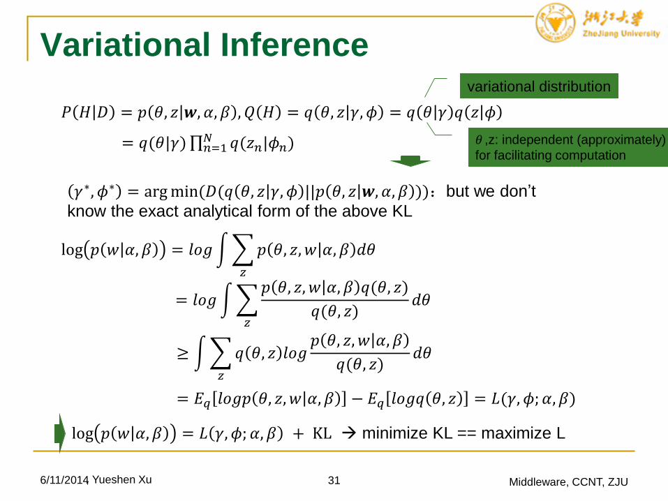
Variational Inference

6/11/2014 31 Middleware, CCNT, ZJU

𝑃 𝐻 𝐷 = 𝑝 𝜃, 𝑧 𝒘, 𝛼, 𝛽 , 𝑄 𝐻 = 𝑞 𝜃, 𝑧 𝛾, 𝜙 = 𝑞 𝜃 𝛾 𝑞 𝑧 𝜙

= 𝑞(𝜃|𝛾) 𝑛=1𝑁 𝑞(𝑧𝑛|𝜙𝑛)

𝛾∗, 𝜙∗ = arg min(𝐷(𝑞 𝜃, 𝑧 𝛾, 𝜙 ||𝑝 𝜃, 𝑧 𝒘, 𝛼, 𝛽 ))：but we don’t

know the exact analytical form of the above KL

log 𝑝 𝑤 𝛼, 𝛽 = 𝑙𝑜𝑔

𝑧

𝑝 𝜃, 𝑧, 𝑤 𝛼, 𝛽 𝑑𝜃

= 𝑙𝑜𝑔

𝑧

𝑝 𝜃, 𝑧, 𝑤 𝛼, 𝛽 𝑞(𝜃, 𝑧)

𝑞(𝜃, 𝑧)𝑑𝜃

≥

𝑧

𝑞 𝜃, 𝑧 𝑙𝑜𝑔𝑝 𝜃, 𝑧, 𝑤 𝛼, 𝛽

𝑞(𝜃, 𝑧)𝑑𝜃

= 𝐸𝑞 𝑙𝑜𝑔𝑝 𝜃, 𝑧, 𝑤 𝛼, 𝛽 − 𝐸𝑞 𝑙𝑜𝑔𝑞 𝜃, 𝑧 = 𝐿(𝛾, 𝜙; 𝛼, 𝛽)

log 𝑝 𝑤 𝛼, 𝛽 = 𝐿 𝛾, 𝜙; 𝛼, 𝛽 + KL minimize KL == maximize L

𝜃 ,z: independent (approximately)

for facilitating computation

, Yueshen Xu

variational distribution

Variational Inference

6/11/2014 32 Middleware, CCNT, ZJU

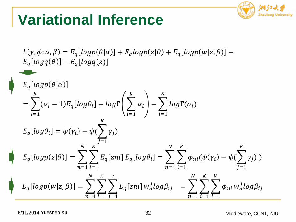
𝐿 𝛾, 𝜙; 𝛼, 𝛽 = 𝐸𝑞 𝑙𝑜𝑔𝑝 𝜃 𝛼 + 𝐸𝑞𝑙𝑜𝑔𝑝 𝑧 𝜃 + 𝐸𝑞 𝑙𝑜𝑔𝑝 𝑤 𝑧, 𝛽 −

𝐸𝑞 𝑙𝑜𝑔𝑞 𝜃 − 𝐸𝑞[𝑙𝑜𝑔𝑞(𝑧)]

𝐸𝑞 𝑙𝑜𝑔𝑝 𝜃 𝛼

=

𝑖=1

𝐾

𝛼𝑖 − 1 𝐸𝑞 𝑙𝑜𝑔𝜃𝑖 + 𝑙𝑜𝑔Γ

𝑖=1

𝐾

𝛼𝑖 −

𝑖=1

𝐾

𝑙𝑜𝑔Γ(𝛼𝑖)

𝐸𝑞 𝑙𝑜𝑔𝜃𝑖 = 𝜓 𝛾𝑖 − 𝜓(

𝑗=1

𝐾

𝛾𝑗)

𝐸𝑞 𝑙𝑜𝑔𝑝 𝑧 𝜃 =

𝑛=1

𝑁

𝑖=1

𝐾

𝐸𝑞[𝑧𝑛𝑖] 𝐸𝑞 𝑙𝑜𝑔𝜃𝑖 =

𝑛=1

𝑁

𝑖=1

𝐾

𝜙𝑛𝑖(𝜓 𝛾𝑖 − 𝜓(

𝑗=1

𝐾

𝛾𝑗) )

𝐸𝑞 𝑙𝑜𝑔𝑝 𝑤 𝑧, 𝛽 =

𝑛=1

𝑁

𝑖=1

𝐾

𝑗=1

𝑉

𝐸𝑞[𝑧𝑛𝑖] 𝑤𝑛𝑗𝑙𝑜𝑔𝛽𝑖𝑗 =

𝑛=1

𝑁

𝑖=1

𝐾

𝑗=1

𝑉

𝜙𝑛𝑖 𝑤𝑛𝑗𝑙𝑜𝑔𝛽𝑖𝑗

, Yueshen Xu

Variational Inference

6/11/2014 33 Middleware, CCNT, ZJU

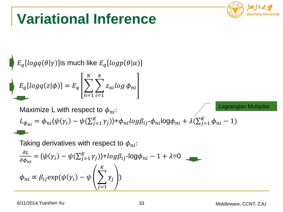
𝐸𝑞 𝑙𝑜𝑔𝑞 𝜃 𝛾 is much like 𝐸𝑞 𝑙𝑜𝑔𝑝 𝜃 𝛼

𝐸𝑞 𝑙𝑜𝑔𝑞 𝑧 𝜙 = 𝐸𝑞

𝑛=1

𝑁

𝑖=1

𝑘

𝑧𝑛𝑖𝑙𝑜𝑔 𝜙𝑛𝑖

Maximize L with respect to 𝜙𝑛𝑖:

𝐿𝜙𝑛𝑖= 𝜙𝑛𝑖(𝜓 𝛾𝑖 − 𝜓( 𝑗=1

𝐾 𝛾𝑗))+𝜙𝑛𝑖𝑙𝑜𝑔𝛽𝑖𝑗-𝜙𝑛𝑖log𝜙𝑛𝑖 + 𝜆( 𝑗=1𝐾 𝜙𝑛𝑖 − 1)

Lagrangian Multiplier

Taking derivatives with respect to 𝜙𝑛𝑖:𝜕𝐿

𝜕𝜙𝑛𝑖= (𝜓 𝛾𝑖 − 𝜓( 𝑗=1

𝐾 𝛾𝑗))+𝑙𝑜𝑔𝛽𝑖𝑗-log𝜙𝑛𝑖 − 1 + 𝜆=0

𝜙𝑛𝑖 ∝ 𝛽𝑖𝑗exp(𝜓 𝛾𝑖 − 𝜓

𝑗=1

𝐾

𝛾𝑗 )

, Yueshen Xu

Variational Inference

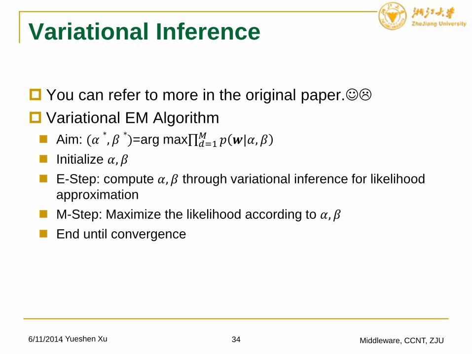
You can refer to more in the original paper.

Variational EM Algorithm

Aim: (𝛼∗, 𝛽

∗)=arg max 𝑑=1

𝑀 𝑝 𝒘|𝛼, 𝛽

Initialize 𝛼, 𝛽

E-Step: compute 𝛼, 𝛽 through variational inference for likelihood

approximation

M-Step: Maximize the likelihood according to 𝛼, 𝛽

End until convergence

6/11/2014 34 Middleware, CCNT, ZJU, Yueshen Xu

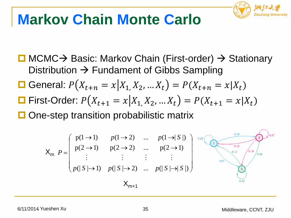
Markov Chain Monte Carlo

MCMC Basic: Markov Chain (First-order) Stationary

Distribution Fundament of Gibbs Sampling

General: 𝑃 𝑋𝑡+𝑛 = 𝑥 𝑋1, 𝑋2, … 𝑋𝑡 = 𝑃(𝑋𝑡+𝑛 = 𝑥|𝑋𝑡)

First-Order: 𝑃 𝑋𝑡+1 = 𝑥 𝑋1, 𝑋2, … 𝑋𝑡 = 𝑃(𝑋𝑡+1 = 𝑥|𝑋𝑡)

One-step transition probabilistic matrix

6/11/2014 35 Middleware, CCNT, ZJU

|)||(|...)2|(|)1|(|

)12(p...)22(p)12(p

|)|1(...)21()11(p

SSpSpSp

Spp

P

Xm

Xm+1

, Yueshen Xu

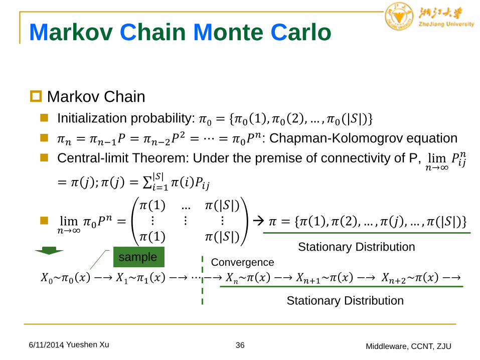
Markov Chain Monte Carlo

Markov Chain

Initialization probability: 𝜋0 = {𝜋0 1 , 𝜋0 2 , … , 𝜋0(|𝑆|)}

𝜋𝑛 = 𝜋𝑛−1𝑃 = 𝜋𝑛−2𝑃2 = ⋯ = 𝜋0𝑃𝑛: Chapman-Kolomogrov equation

Central-limit Theorem: Under the premise of connectivity of P, lim𝑛→∞

𝑃𝑖𝑗𝑛

= 𝜋 𝑗 ; 𝜋 𝑗 = 𝑖=1|𝑆|

𝜋 𝑖 𝑃𝑖𝑗

lim𝑛→∞

𝜋0𝑃𝑛 =𝜋(1) … 𝜋(|𝑆|)

⋮ ⋮ ⋮𝜋(1) 𝜋(|𝑆|)

𝜋 = {𝜋 1 , 𝜋 2 , … , 𝜋 𝑗 , … , 𝜋(|𝑆|)}

6/11/2014 36 Middleware, CCNT, ZJU

Stationary Distribution

𝑋0~𝜋0 𝑥 −→ 𝑋1~𝜋1 𝑥 −→ ⋯ −→ 𝑋𝑛~𝜋 𝑥 −→ 𝑋𝑛+1~𝜋 𝑥 −→ 𝑋𝑛+2~𝜋 𝑥 −→

sample Convergence

Stationary Distribution

, Yueshen Xu

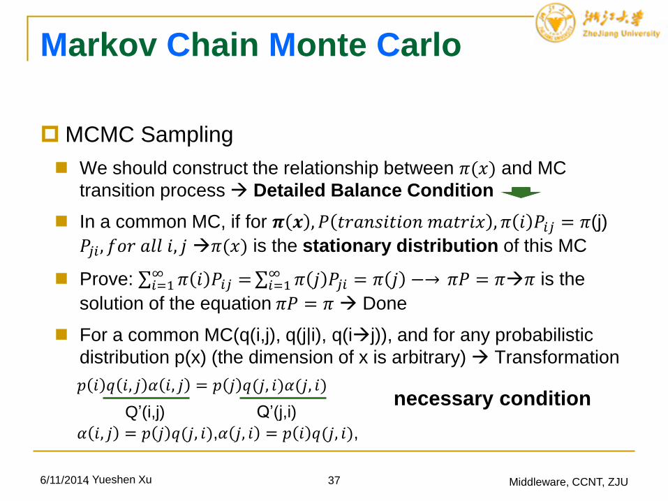
Markov Chain Monte Carlo

MCMC Sampling

We should construct the relationship between 𝜋(𝑥) and MC

transition process Detailed Balance Condition

In a common MC, if for 𝝅 𝒙 , 𝑃 𝑡𝑟𝑎𝑛𝑠𝑖𝑡𝑖𝑜𝑛 𝑚𝑎𝑡𝑟𝑖𝑥 , 𝜋 𝑖 𝑃𝑖𝑗 = 𝜋(j)

𝑃𝑗𝑖 , 𝑓𝑜𝑟 𝑎𝑙𝑙 𝑖, 𝑗 𝜋(𝑥) is the stationary distribution of this MC

Prove: 𝑖=1∞ 𝜋 𝑖 𝑃𝑖𝑗 = 𝑖=1

∞ 𝜋 𝑗 𝑃𝑗𝑖 = 𝜋 𝑗 −→ 𝜋𝑃 = 𝜋𝜋 is the

solution of the equation 𝜋𝑃 = 𝜋 Done

For a common MC(q(i,j), q(j|i), q(ij)), and for any probabilistic

distribution p(x) (the dimension of x is arbitrary) Transformation

6/11/2014 37 Middleware, CCNT, ZJU

𝑝 𝑖 𝑞 𝑖, 𝑗 𝛼 𝑖, 𝑗 = 𝑝 𝑗 𝑞(𝑗, 𝑖)𝛼(𝑗, 𝑖)

Q’(i,j) Q’(j,i)

𝛼 𝑖, 𝑗 = 𝑝 𝑗 𝑞(𝑗, 𝑖),𝛼 𝑗, 𝑖 = 𝑝 𝑖 𝑞(𝑗, 𝑖),

necessary condition

, Yueshen Xu

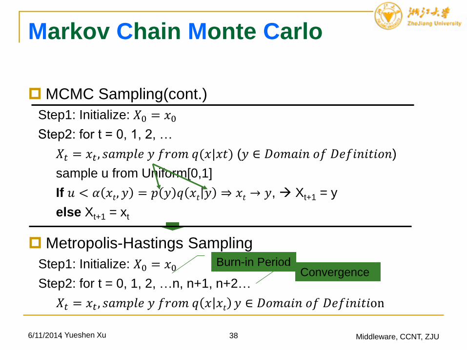
Markov Chain Monte Carlo

MCMC Sampling(cont.)

Step1: Initialize: 𝑋0 = 𝑥0

Step2: for t = 0, 1, 2, …

𝑋𝑡 = 𝑥𝑡 , 𝑠𝑎𝑚𝑝𝑙𝑒 𝑦 𝑓𝑟𝑜𝑚 𝑞(𝑥|𝑥𝑡) (𝑦 ∈ 𝐷𝑜𝑚𝑎𝑖𝑛 𝑜𝑓 𝐷𝑒𝑓𝑖𝑛𝑖𝑡𝑖𝑜𝑛)

sample u from Uniform[0,1]

If 𝑢 < 𝛼 𝑥𝑡, 𝑦 = 𝑝 𝑦 𝑞 𝑥𝑡 𝑦 ⇒ 𝑥𝑡 → 𝑦, Xt+1 = y

else Xt+1 = xt

6/11/2014 38 Middleware, CCNT, ZJU

Metropolis-Hastings Sampling

Step1: Initialize: 𝑋0 = 𝑥0

Step2: for t = 0, 1, 2, …n, n+1, n+2…

𝑋𝑡 = 𝑥𝑡 , 𝑠𝑎𝑚𝑝𝑙𝑒 𝑦 𝑓𝑟𝑜𝑚 𝑞 𝑥 𝑥𝑡 𝑦 ∈ 𝐷𝑜𝑚𝑎𝑖𝑛 𝑜𝑓 𝐷𝑒𝑓𝑖𝑛𝑖𝑡𝑖on

Burn-in PeriodConvergence

, Yueshen Xu

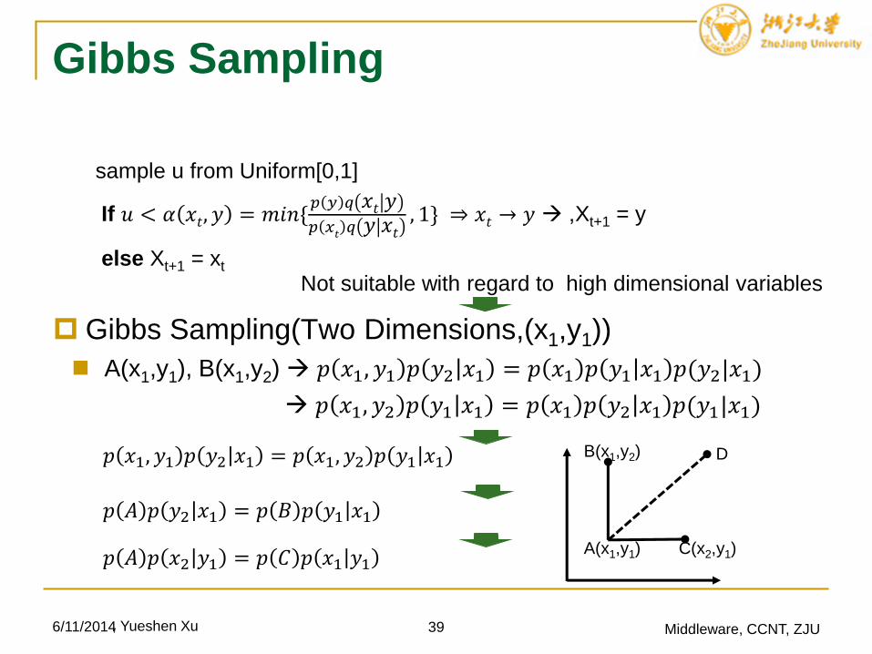
Gibbs Sampling

sample u from Uniform[0,1]

If 𝑢 < 𝛼 𝑥𝑡, 𝑦 = 𝑚𝑖𝑛{𝑝 𝑦 𝑞 𝑥𝑡 𝑦𝑝 𝑥

𝑡𝑞 𝑦 𝑥𝑡

, 1} ⇒ 𝑥𝑡 → 𝑦 , Xt+1 = y

else Xt+1 = xt

6/11/2014 39 Middleware, CCNT, ZJU

Not suitable with regard to high dimensional variables

Gibbs Sampling(Two Dimensions,(x1,y1))

A(x1,y1), B(x1,y2) 𝑝 𝑥1, 𝑦1 𝑝 𝑦2 𝑥1 = 𝑝 𝑥1 𝑝 𝑦1 𝑥1 𝑝(𝑦2|𝑥1)

𝑝 𝑥1, 𝑦2 𝑝 𝑦1 𝑥1 = 𝑝 𝑥1 𝑝 𝑦2 𝑥1 𝑝(𝑦1|𝑥1)

𝑝 𝑥1, 𝑦1 𝑝 𝑦2 𝑥1 = 𝑝 𝑥1, 𝑦2 𝑝 𝑦1 𝑥1

𝑝 𝐴 𝑝 𝑦2 𝑥1 = 𝑝 𝐵 𝑝 𝑦1 𝑥1

A(x1,y1)

B(x1,y2)

C(x2,y1)

D

𝑝 𝐴 𝑝 𝑥2 𝑦1 = 𝑝 𝐶 𝑝 𝑥1 𝑦1

, Yueshen Xu

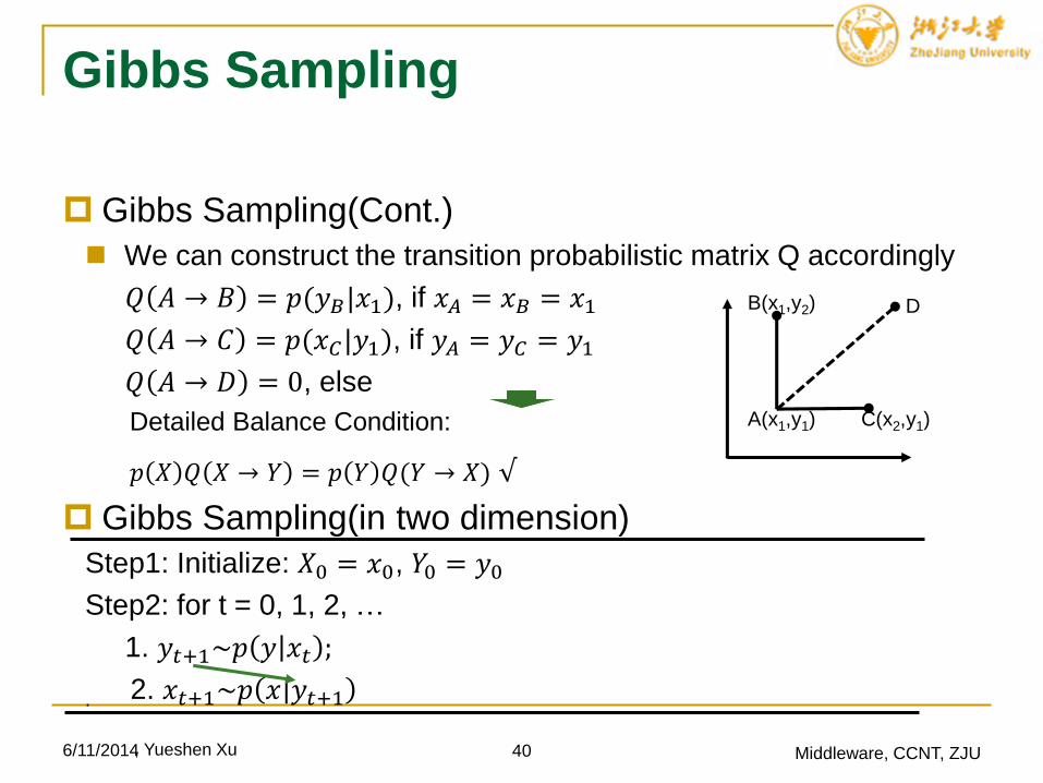
Gibbs Sampling

Gibbs Sampling(Cont.)

We can construct the transition probabilistic matrix Q accordingly

𝑄 𝐴 → 𝐵 = 𝑝(𝑦𝐵|𝑥1), if 𝑥𝐴 = 𝑥𝐵 = 𝑥1

𝑄 𝐴 → 𝐶 = 𝑝(𝑥𝐶|𝑦1), if 𝑦𝐴 = 𝑦𝐶 = 𝑦1

𝑄 𝐴 → 𝐷 = 0, else

6/11/2014 40 Middleware, CCNT, ZJU

A(x1,y1)

B(x1,y2)

C(x2,y1)

D

Detailed Balance Condition:

𝑝 𝑋 𝑄 𝑋 → 𝑌 = 𝑝 𝑌 𝑄(𝑌 → 𝑋) √

Gibbs Sampling(in two dimension)

Step1: Initialize: 𝑋0 = 𝑥0, 𝑌0 = 𝑦0

Step2: for t = 0, 1, 2, …

1. 𝑦𝑡+1~𝑝 𝑦 𝑥𝑡 ;

. 2. 𝑥𝑡+1~𝑝 𝑥 𝑦𝑡+1

, Yueshen Xu

Gibbs Sampling

6/11/2014 41 Middleware, CCNT, ZJU

Gibbs Sampling(in two dimension)

Step1: Initialize: 𝑋0 = 𝑥0 = {𝑥1: 𝑖 = 1,2, … 𝑛}

Step2: for t = 0, 1, 2, …

1. 𝑥1(𝑡+1)

~𝑝 𝑥1 𝑥2(𝑡)

, 𝑥3(𝑡)

, … , 𝑥𝑛(𝑡)

;

2. 𝑥2𝑡+1~𝑝 𝑥2 𝑥1

(𝑡+1), 𝑥3

(𝑡), … , 𝑥𝑛

(𝑡)

3. …

4. 𝑥𝑗𝑡+1~𝑝 𝑥𝑗 𝑥1

(𝑡+1), 𝑥𝑗−1

(𝑡+1), 𝑥𝑗+1

(𝑡)… , 𝑥𝑛

(𝑡)

5. …

6. 𝑥𝑛𝑡+1~𝑝 𝑥𝑛 𝑥1

(𝑡+1), 𝑥2

(𝑡+1), … , 𝑥𝑛−1

(𝑡+1)

t+1 t

, Yueshen Xu

Gibbs Sampling for LDA

Gibbs Sampling in LDA

Dir 𝑝 𝛼 =1

Δ(𝛼) 𝑘=1

𝑉 𝑝𝑘𝛼𝑘−1

, Δ( 𝛼) is the normalization factor:

Δ 𝛼 = 𝑘=1𝑉 𝑝𝑘

𝛼𝑘−1𝑑 𝑝

𝑝 𝑧𝑚 𝛼 = 𝑝 𝑧𝑚 𝜃 𝑝 𝜃 𝛼 𝑑 𝑝 = 𝑘=1

𝑉 𝜃𝑘𝑛𝑘Dir( 𝜃| 𝛼) 𝑑 𝜃

= 𝑘=1𝑉 𝜃𝑘

𝑛𝑘 1

Δ(𝛼) 𝑘=1

𝑉 𝜃𝑘𝛼𝑘−1

𝑑 𝜃

= 1

Δ(𝛼) 𝑘=1

𝑉 𝜃𝑘𝑛𝑘+𝛼𝑘−1

𝑑 𝜃 =Δ(𝑛𝑚+𝛼)

Δ(𝛼)

6/11/2014 42 Middleware, CCNT, ZJU

𝑝 𝒛 𝛼 = 𝑚=1𝑀 𝑝 𝑧𝑚 𝛼 = 𝑚=1

𝑀 Δ(𝑛𝑚+𝛼)

Δ(𝛼)−→

𝑝 𝒘, 𝒛 𝛼, 𝛽 = 𝑘=1𝐾 Δ(𝑛𝑘+𝛽)

Δ(𝛽) 𝑚=1

𝑀 Δ(𝑛𝑚+𝛼)

Δ(𝛼)

, Yueshen Xu

Gibbs Sampling for LDA

Gibbs Sampling in LDA

𝑝 𝜃𝑚 𝑧¬𝑖,𝑤¬𝑖 = 𝐷𝑖𝑟(𝜃𝑚|𝑛𝑚,¬𝑖 + 𝛼), 𝑝 𝜑𝑘 𝑧¬𝑖,𝑤¬𝑖 =

𝐷𝑖𝑟(𝜑𝑘|𝑛𝑘,¬𝑖 + 𝛽)

𝑝(𝑧𝑖 = 𝑘| 𝑧¬𝑖,𝑤¬𝑖) ∝ 𝑝 𝑧𝑖 = 𝑘, 𝑤𝑖 = 𝑡, 𝜃𝑚, 𝜑𝑘 𝑧¬𝑖,𝑤¬𝑖 = 𝐸 𝜃𝑚𝑘 ∙

𝐸 𝜑𝑘𝑡 = 𝜃𝑚𝑘 ∙ 𝜑𝑘𝑡

𝜃𝑚𝑘=𝑛𝑚,¬𝑖

(𝑡)+𝛼𝑘

𝑘=1𝐾 (𝑛

𝑚,¬𝑖(𝑘)

+𝛼𝑘), 𝜑𝑘𝑡=

𝑛𝑘,¬𝑖(𝑡)

+𝛽𝑘

𝑡=1𝑉 (𝑛

𝑘,¬𝑖(𝑡)

+𝛽𝑘)

𝑝(𝑧𝑖 = 𝑘| 𝑧¬𝑖,𝑤) ∝𝑛𝑚,¬𝑖

(𝑡)+𝛼𝑘

𝑘=1𝐾 (𝑛𝑚,¬𝑖

(𝑘)+𝛼𝑘)

×𝑛𝑘,¬𝑖

(𝑡)+𝛽𝑘

𝑡=1𝑉 (𝑛𝑘,¬𝑖

(𝑡)+𝛽𝑘)

𝑧𝑖(𝑡+1)

~ 𝑝(𝑧𝑖 = 𝑘| 𝑧¬𝑖,𝑤), i=1…K

6/11/2014 43 Middleware, CCNT, ZJU, Yueshen Xu

Q&A

6/11/2014 Middleware, CCNT, ZJU44, Yueshen Xu