


Languages
Pages
Legal

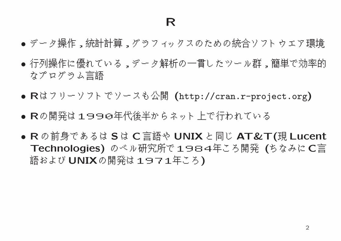
R
• データ操作,統計計算,グラフィックスのための統合ソフトウエア環境• 行列操作に優れている,データ解析の一貫したツール群,簡単で効率的なプログラム言語
• Rはフリーソフトでソースも公開 (http://cran.r-project.org)
• Rの開発は1990年代後半からネット上で行われている
• Rの前身であるは Sは C言語やUNIXと同じ AT&T(現LucentTechnologies) のベル研究所で1984年ころ開発 (ちなみにC言語およびUNIXの開発は1971年ころ)
2
講義内容
「データ解析」では統計処理ソフトウエアであるRを用いた多変量解析の実践的な講義を行う.Rの使用法について簡単に紹介した後,実際にRを使ったデータ解析を行う.単にソフトの使用法を学ぶのではなく,その背後にある数学を自分のものにすることが目標である.回帰分析や主成分分析のためのR関数を自分自身で書き,それを使ってデータ解析を行うのである.この経験は将来未知の問題で新しい手法を開発する場面で役に立つだろう.
3

講義予定
R入門 (1)端末室での演習1 (2)Rによる線形代数 (3)回帰分析 (4,5)主成分分析 (6,7)端末室での演習2 (8)クラスター分析 (9)正準相関分析 (10)判別分析 (11)モデル選択 (12)ブートストラップ法 (13)端末室での演習3 (14)
4

講義について
• ホームページhttp://www.is.titech.ac.jp/~shimo/class/
• 担当:下平• ティーチングアシスタント: 坂口,多賀
• 評価方法: 出席とレポート
• 質問受け付け: まずティーチングアシスタントに質問内容のメールを出すこと.面談が必要な場合はあらかじめメールにてアポイントを取ること.もしくは講義か演習時に直接質問する.
5
eduでのRの利用の準備
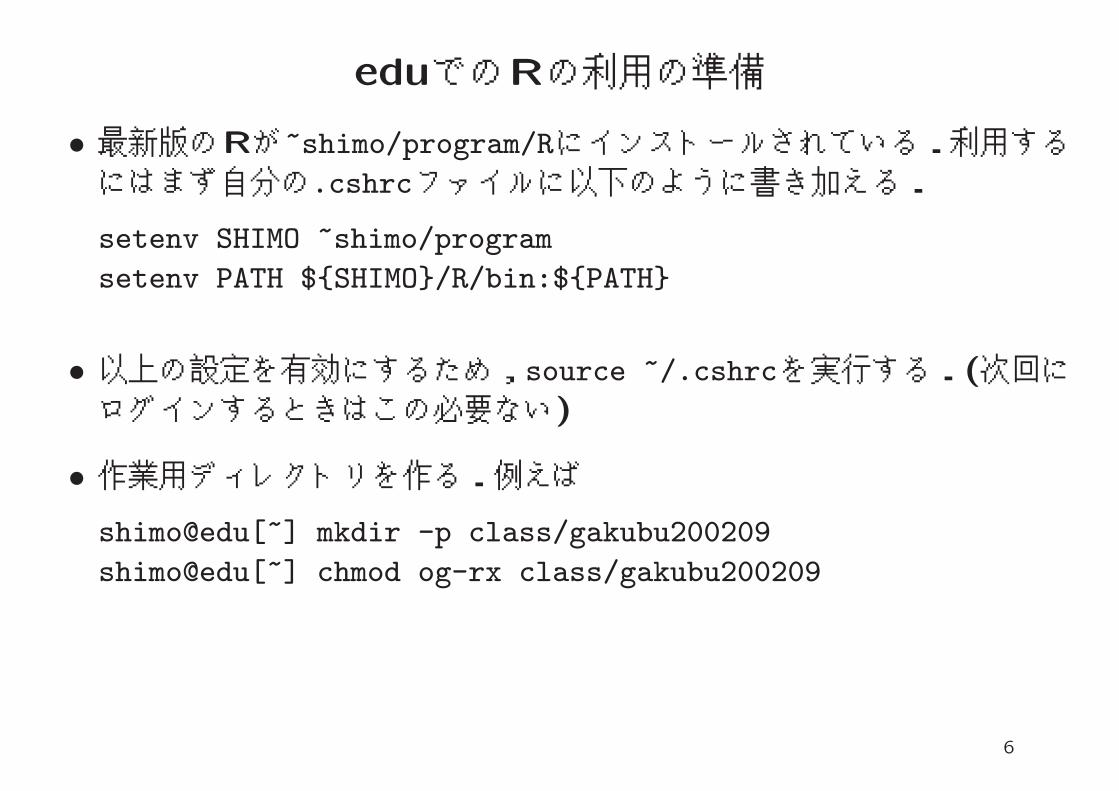
• 最新版のRが~shimo/program/Rにインストールされている.利用するにはまず自分の.cshrcファイルに以下のように書き加える.
setenv SHIMO ~shimo/program
setenv PATH ${SHIMO}/R/bin:${PATH}
• 以上の設定を有効にするため,source ~/.cshrcを実行する.(次回にログインするときはこの必要ない)
• 作業用ディレクトリを作る.例えばshimo@edu[~] mkdir -p class/gakubu200209
shimo@edu[~] chmod og-rx class/gakubu200209
6

eduでのRの利用
• 作業用ディレクトリに移動しRを起動
shimo@edu[~] cd class/gakubu200209
shimo@edu[gakubu200209] R
• たとえば sin(x)の曲線を描く
> x <- seq(0,10,0.1)
> plot(x,sin(x),type="l")
• Rの終了は q()コマンド
> q()
Save workspace image? [y/n/c]: y
• 作業用ディレクトリにファイル.RDataが自動的に作られる.7

emacsでの統合環境 ESS
• .emacsファイルに以下を書き加えてからemacsを再起動.
;;; ess
(setq load-path (cons
(expand-file-name "~shimo/program/ess/lisp") load-path ))
(autoload ’R "ess-site" "" t)
(add-hook ’ess-post-run-hook (function (lambda ()
(set-buffer-process-coding-system ’euc-japan ’euc-japan))))
• emacs内でM-x RによってRを起動する.
• セッションはC-x C-wによってxxxx.Rtのような名前でセーブする.
• プログラムのファイルはyyyy.Rのような名前で作成しRコマンドsource ("yyyy.R")でロード.
• RのヘルプはC-c C-vで別ウィンドウが開く8

講義で用いるデータセット
総務庁統計局統計センターが公開している社会・人口統計体系http://www.stat.go.jp/data/ssds/index.htm
edu:~shimo/class/gakubu200209/data/X2000.R
というファイルでX2000というリスト型の変数を定義している.
X2000$x [データ本体] サイズ47×1173の行列X2000$item [項目名] サイズ1173の文字型ベクトルX2000$jitem (日本語)X2000$pref [県名] サイズ47の文字型ベクトルX2000$jpref (日本語)
9

項目例
1 A05201 自然増加率2 A06102 一般世帯の平均人員3 A06202 核家族世帯割合4 F01503 共働き世帯割合5 A06205 単独世帯割合6 A06301 65歳以上の親族のいる世帯割合7 A06302 高齢夫婦のみの世帯の割合8 A06304 高齢単身世帯の割合9 A06601 婚姻率(人口千人当たり)
10 A06602 離婚率(人口千人当たり)
10

データ行列の一部
A05201 A06102 A06202 F01503 · · ·Hokkaido 0.04 2.42 60.54 26.54 · · ·Aomori -0.02 2.86 54.20 34.38 · · ·Iwate -0.07 2.92 50.87 38.82 · · ·Miyagi 0.18 2.80 51.96 31.88 · · ·Akita -0.25 3.00 50.48 39.55 · · ·Yamagata -0.12 3.25 45.79 47.09 · · ·Fukushima 0.06 3.05 52.12 39.53 · · ·Ibaraki 0.16 2.99 58.28 35.84 · · ·Tochigi 0.13 2.97 56.47 37.59 · · ·Gumma 0.12 2.88 60.07 36.35 · · ·Saitama 0.36 2.78 65.46 30.89 · · ·Chiba 0.27 2.70 62.55 29.57 · · ·Tokyo 0.11 2.21 52.15 22.09 · · ·Kanagawa 0.36 2.53 62.04 25.04 · · ·
. . . . .
. . . . .
. . . . .Okinawa 0.67 2.91 64.54 25.70 · · ·
11

サンプルセッション
西7号館端末室(edu)で演習する.セッションファイルと同じことを自分でやってみる.詳しい意味は分からなくても良い.データ解析とRについて慣れることが目的.
• サンプルセッション1Rによるデータ解析1(主成分分析,クラスタリング,重回帰分析)ファイル: ~shimo/class/gakubu200209/note20020919a.Rt
• サンプルセッション2Rによるデータ解析2(ランダムにデータ項目を選ぶ)ファイル: ~shimo/class/gakubu200209/note20020919b.Rt
• サンプルセッション3R言語入門ファイル: ~shimo/class/gakubu200209/note20020919c.Rt
12

サンプルセッション1
Last login: Fri Sep 20 2002 15:54:22 +0900 from grandma
Sun Microsystems Inc. SunOS 5.8 Generic Patch October 2001
No mail.
Sun Microsystems Inc. SunOS 5.8 Generic Patch October 2001
shimo@edu[~] cd class/gakubu200209
shimo@edu[gakubu200209] R
R : Copyright 2002, The R Development Core Team
Version 1.5.1 Patched (2002-09-08)
R is free software and comes with ABSOLUTELY NO WARRANTY.
You are welcome to redistribute it under certain conditions.
Type ‘license()’ or ‘licence()’ for distribution details.
R is a collaborative project with many contributors.
Type ‘contributors()’ for more information.
13

Type ‘demo()’ for some demos, ‘help()’ for on-line help, or
‘help.start()’ for a HTML browser interface to help.
Type ‘q()’ to quit R.
[Previously saved workspace restored]
> source("~shimo/class/gakubu200209/data/X2000.R")
> names(X2000)
[1] "x" "pref" "code" "item" "cate" "clab" "jpref" "jitem" "junit"
[10] "jcate" "rm"
> dim(X2000$x)
[1] 47 1173
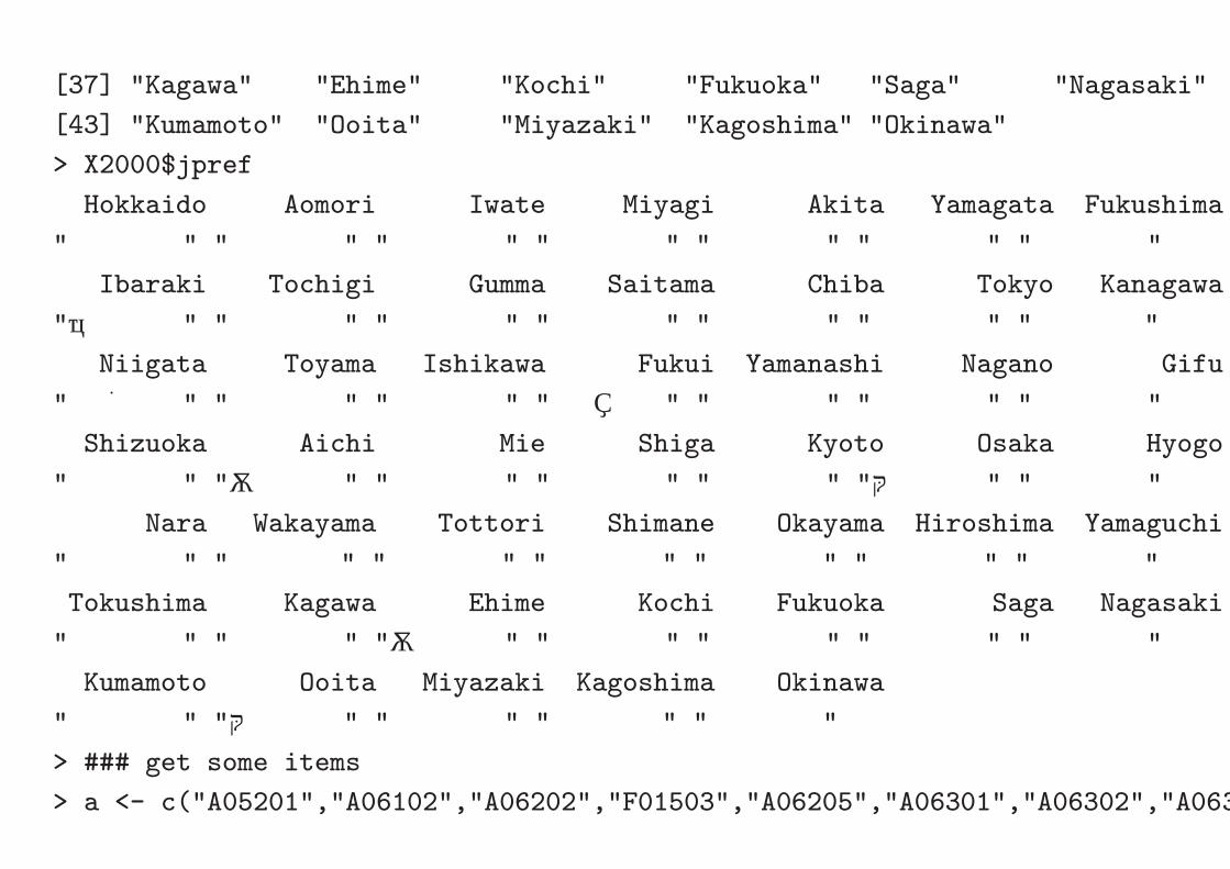
> X2000$pref
[1] "Hokkaido" "Aomori" "Iwate" "Miyagi" "Akita" "Yamagata"
[7] "Fukushima" "Ibaraki" "Tochigi" "Gumma" "Saitama" "Chiba"
[13] "Tokyo" "Kanagawa" "Niigata" "Toyama" "Ishikawa" "Fukui"
[19] "Yamanashi" "Nagano" "Gifu" "Shizuoka" "Aichi" "Mie"
[25] "Shiga" "Kyoto" "Osaka" "Hyogo" "Nara" "Wakayama"
[31] "Tottori" "Shimane" "Okayama" "Hiroshima" "Yamaguchi" "Tokushima"
[37] "Kagawa" "Ehime" "Kochi" "Fukuoka" "Saga" "Nagasaki"
[43] "Kumamoto" "Ooita" "Miyazaki" "Kagoshima" "Okinawa"
> X2000$jpref
Hokkaido Aomori Iwate Miyagi Akita Yamagata Fukushima
"北 海 道" "青 森 県" "岩 手 県" "宮 城 県" "秋 田 県" "山 形 県" "福 島 県"
Ibaraki Tochigi Gumma Saitama Chiba Tokyo Kanagawa
"茨 城 県" "栃 木 県" "群 馬 県" "埼 玉 県" "千 葉 県" "東 京 都" "神奈川県"
Niigata Toyama Ishikawa Fukui Yamanashi Nagano Gifu
"新 潟 県" "富 山 県" "石 川 県" "福 井 県" "山 梨 県" "長 野 県" "岐 阜 県"
Shizuoka Aichi Mie Shiga Kyoto Osaka Hyogo
"静 岡 県" "愛 知 県" "三 重 県" "滋 賀 県" "京 都 府" "大 阪 府" "兵 庫 県"
Nara Wakayama Tottori Shimane Okayama Hiroshima Yamaguchi
"奈 良 県" "和歌山県" "鳥 取 県" "島 根 県" "岡 山 県" "広 島 県" "山 口 県"
Tokushima Kagawa Ehime Kochi Fukuoka Saga Nagasaki
"徳 島 県" "香 川 県" "愛 媛 県" "高 知 県" "福 岡 県" "佐 賀 県" "長 崎 県"
Kumamoto Ooita Miyazaki Kagoshima Okinawa
"熊 本 県" "大 分 県" "宮 崎 県" "鹿児島県" "沖 縄 県"
> ### get some items
> a <- c("A05201","A06102","A06202","F01503","A06205","A06301","A06302","A063

> X2000$item[a]
A05201
"Rate of natural increase "
A06102
"Members per private household "
A06202
"Ratio of family nuclei households "
F01503
"Ratio of dual-income households "
A06205
"Ratio of one-person households "
A06301
"Ratio of households with members65 years old and over "
A06302
"Ratio of aged-couple households "
A06304
"Ratio of aged-single person households "
A06601
"Rate of marriages (per 1,000 persons) "

A06602
"Rate of divorces (per 1,000 persons) "
> X2000$jitem[a]
A05201 A06102
"自 然 増 加 率 " "一 般 世 帯 の 平 均 人 員 "
A06202 F01503
"核 家 族 世 帯 割 合 " "共 働 き 世 帯 割 合 "
A06205 A06301
"単 独 世 帯 割 合 " "65歳以上の親族のいる世帯割合 "
A06302 A06304
"高齢夫婦のみの世帯の割合 " "高 齢 単 身 世 帯 の 割 合 "
A06601 A06602
"婚 姻 率 (人口千人当たり) " "離 婚 率 (人口千人当たり) "
> na <- paste(seq(along=a),a,X2000$item[a])
> na
[1] "1 A05201 Rate of natural increase "
[2] "2 A06102 Members per private household "
[3] "3 A06202 Ratio of family nuclei households "
[4] "4 F01503 Ratio of dual-income households "

[5] "5 A06205 Ratio of one-person households "
[6] "6 A06301 Ratio of households with members65 years old and over "
[7] "7 A06302 Ratio of aged-couple households "
[8] "8 A06304 Ratio of aged-single person households "
[9] "9 A06601 Rate of marriages (per 1,000 persons) "
[10] "10 A06602 Rate of divorces (per 1,000 persons) "
> jna <- paste(seq(along=a),a,X2000$jitem[a])
> jna
[1] "1 A05201 自 然 増 加 率 "
[2] "2 A06102 一 般 世 帯 の 平 均 人 員 "
[3] "3 A06202 核 家 族 世 帯 割 合 "
[4] "4 F01503 共 働 き 世 帯 割 合 "
[5] "5 A06205 単 独 世 帯 割 合 "
[6] "6 A06301 65歳以上の親族のいる世帯割合 "
[7] "7 A06302 高齢夫婦のみの世帯の割合 "
[8] "8 A06304 高 齢 単 身 世 帯 の 割 合 "
[9] "9 A06601 婚 姻 率 (人口千人当たり) "
[10] "10 A06602 離 婚 率 (人口千人当たり) "
> x <- X2000$x[,a]

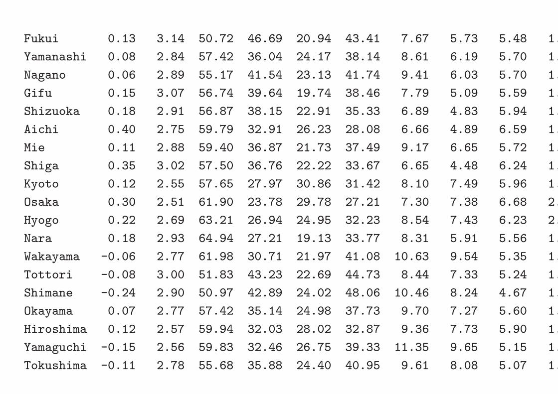
> x
A05201 A06102 A06202 F01503 A06205 A06301 A06302 A06304 A06601 A066
Hokkaido 0.04 2.42 60.54 26.54 29.95 30.50 9.90 7.39 5.77 2.
Aomori -0.02 2.86 54.20 34.38 24.08 38.99 7.45 6.61 5.24 1.
Iwate -0.07 2.92 50.87 38.82 24.47 42.42 7.87 6.05 5.14 1.
Miyagi 0.18 2.80 51.96 31.88 28.59 33.04 6.42 4.54 5.79 1.
Akita -0.25 3.00 50.48 39.55 21.24 47.77 9.15 6.71 4.69 1.
Yamagata -0.12 3.25 45.79 47.09 19.98 49.75 7.50 5.27 5.40 1.
Fukushima 0.06 3.05 52.12 39.53 22.60 41.70 7.58 5.65 5.44 1.
Ibaraki 0.16 2.99 58.28 35.84 21.42 33.95 6.35 4.31 5.78 1.
Tochigi 0.13 2.97 56.47 37.59 22.42 34.95 6.28 4.69 5.87 1.
Gumma 0.12 2.88 60.07 36.35 21.78 35.61 7.95 5.49 5.73 1.
Saitama 0.36 2.78 65.46 30.89 23.15 25.10 5.89 3.94 6.19 2.
Chiba 0.27 2.70 62.55 29.57 25.45 26.75 6.36 4.51 6.30 2.
Tokyo 0.11 2.21 52.15 22.09 40.85 25.44 6.69 7.23 6.87 2.
Kanagawa 0.36 2.53 62.04 25.04 29.54 24.74 6.81 5.04 6.89 2.
Niigata -0.03 3.07 51.07 43.22 21.69 43.77 7.82 5.27 5.03 1.
Toyama -0.01 3.09 52.30 46.09 19.93 43.47 7.89 5.59 5.51 1.
Ishikawa 0.12 2.83 53.17 40.23 25.98 36.29 7.64 5.81 5.86 1.
Fukui 0.13 3.14 50.72 46.69 20.94 43.41 7.67 5.73 5.48 1.
Yamanashi 0.08 2.84 57.42 36.04 24.17 38.14 8.61 6.19 5.70 1.
Nagano 0.06 2.89 55.17 41.54 23.13 41.74 9.41 6.03 5.70 1.
Gifu 0.15 3.07 56.74 39.64 19.74 38.46 7.79 5.09 5.59 1.
Shizuoka 0.18 2.91 56.87 38.15 22.91 35.33 6.89 4.83 5.94 1.
Aichi 0.40 2.75 59.79 32.91 26.23 28.08 6.66 4.89 6.59 1.
Mie 0.11 2.88 59.40 36.87 21.73 37.49 9.17 6.65 5.72 1.
Shiga 0.35 3.02 57.50 36.76 22.22 33.67 6.65 4.48 6.24 1.
Kyoto 0.12 2.55 57.65 27.97 30.86 31.42 8.10 7.49 5.96 1.
Osaka 0.30 2.51 61.90 23.78 29.78 27.21 7.30 7.38 6.68 2.
Hyogo 0.22 2.69 63.21 26.94 24.95 32.23 8.54 7.43 6.23 2.
Nara 0.18 2.93 64.94 27.21 19.13 33.77 8.31 5.91 5.56 1.
Wakayama -0.06 2.77 61.98 30.71 21.97 41.08 10.63 9.54 5.35 1.
Tottori -0.08 3.00 51.83 43.23 22.69 44.73 8.44 7.33 5.24 1.
Shimane -0.24 2.90 50.97 42.89 24.02 48.06 10.46 8.24 4.67 1.
Okayama 0.07 2.77 57.42 35.14 24.98 37.73 9.70 7.27 5.60 1.
Hiroshima 0.12 2.57 59.94 32.03 28.02 32.87 9.36 7.73 5.90 1.
Yamaguchi -0.15 2.56 59.83 32.46 26.75 39.33 11.35 9.65 5.15 1.
Tokushima -0.11 2.78 55.68 35.88 24.40 40.95 9.61 8.08 5.07 1.

Kagawa 0.03 2.75 58.53 36.35 23.81 38.88 9.95 7.59 5.63 1.
Ehime -0.08 2.59 60.33 31.24 26.30 38.15 11.03 9.06 5.12 1.
Kochi -0.25 2.47 57.67 33.12 29.85 40.21 10.98 11.16 5.00 2.
Fukuoka 0.14 2.57 57.86 26.51 30.24 31.10 7.88 7.48 5.94 2.
Saga 0.07 3.08 55.06 39.49 20.96 42.83 8.27 6.99 5.19 1.
Nagasaki 0.02 2.71 59.92 31.00 25.30 39.10 9.84 9.18 5.12 1.
Kumamoto 0.02 2.81 56.19 34.98 25.04 40.22 9.52 7.96 5.15 1.
Ooita -0.06 2.64 58.01 32.47 26.42 39.43 10.79 8.93 5.08 1.
Miyazaki 0.07 2.61 62.18 35.51 25.74 36.93 11.13 9.11 5.32 2.
Kagoshima -0.13 2.43 62.44 29.85 30.12 38.01 12.66 12.39 5.09 1.
Okinawa 0.67 2.91 64.54 25.70 24.26 27.92 5.39 6.22 6.47 2.
> dim(x)
[1] 47 10
> # load "mybiplot", "mylsfit", "mypca", "myplot", "mysvd", "psinit"
> source("~shimo/class/gakubu200209/myfunc20020919.R")
>
主成分分析
主成分分析 = PCA (principal component analysis)
• 多変量解析の定番• データの変動をできるだけ少数個の変換された変量で説明• 主成分=変換された変量• バイプロットによって結果を視覚的に示す
14

PCAの関数
mypca <- function(dat) {
s <- mysvd(dat)
x <- s$u %*% diag(s$d)
y <- s$v %*% diag(s$d)
list(x=x,y=y,d=s$d,u=s$u,v=s$v)
}
> p <- mypca(scale(x))
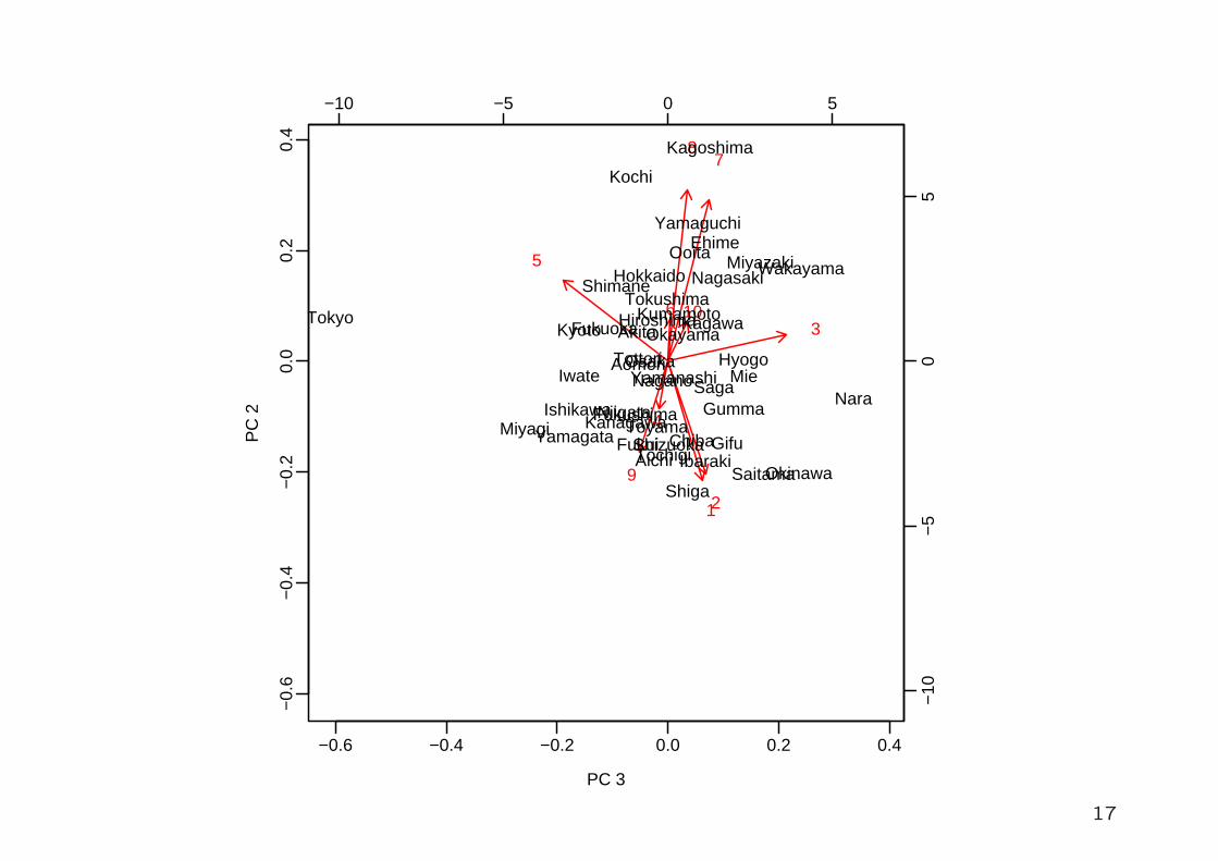
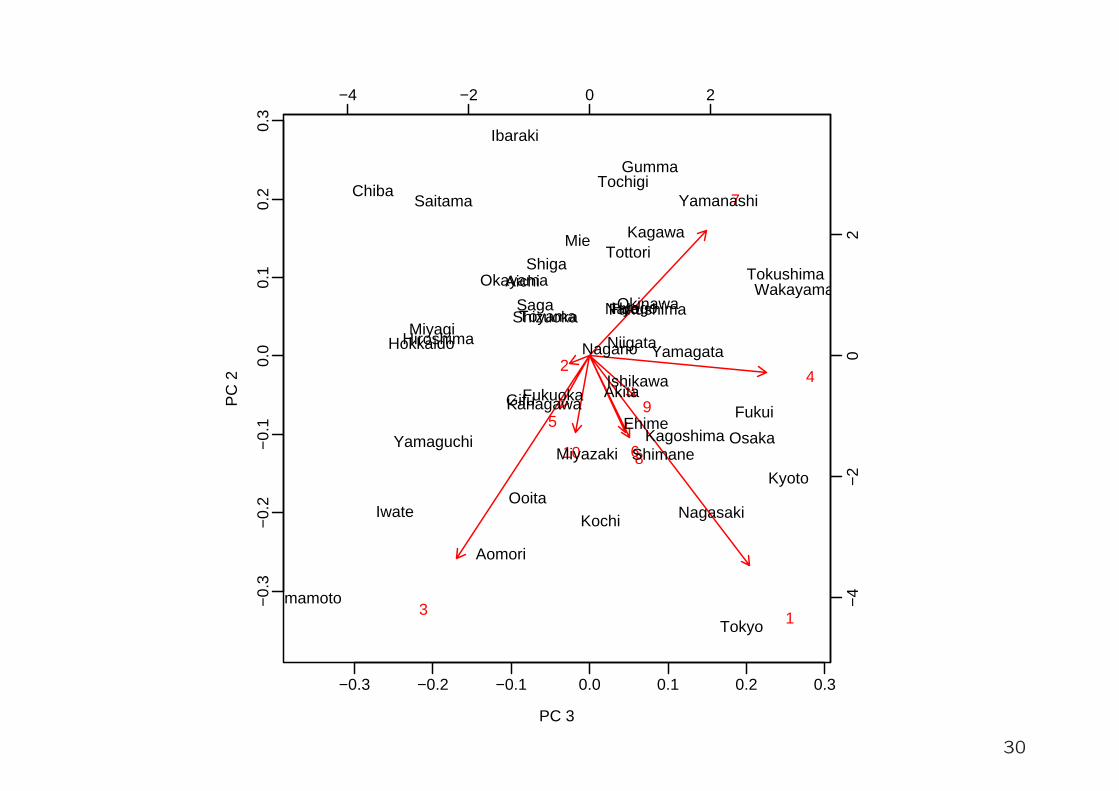
> mybiplot(p$u,p$y)
> mybiplot(p$u,p$y,choi=3:2)
15

−0.3 −0.2 −0.1 0.0 0.1 0.2 0.3 0.4
−0.
3−
0.2
−0.
10.
00.
10.
20.
30.
4
PC 1
PC
2
−5 0 5
−5
05
1 A05201 Rate of natu2 A06102 Members per private household
3 A06202 Ratio of fam
4 F01503 Ratio of dual−income households
5 A06205 Ratio of one−
6 A06301 Ratio of households with members65 years old and over
7 A06302 Ratio of aged−couple households 8 A06304 Ratio of aged−single person hous
9 A06601 Rate of m
10 A06602 Rate
Hokkaido
AomoriIwate
Miyagi
Akita
Yamagata
Fukushima
IbarakiTochigi
Gumma
Saitama
Chiba
Tokyo
KanagawaNiigata
Toyama
Ishikawa
Fukui
YamanashiNagano
Gifu ShizuokaAichi
Mie
Shiga
Kyoto
OsakaHyogo
Nara
Wakayama
Tottori
Shimane
OkayamaHiroshima
Yamaguchi
Tokushima
Kagawa
Ehime
Kochi
Fukuoka
Saga
Nagasaki
Kumamoto
OoitaMiyazaki
Kagoshima
Okinawa
16
−0.6 −0.4 −0.2 0.0 0.2 0.4
−0.
6−
0.4
−0.
20.
00.
20.
4
PC 3
PC
2
−10 −5 0 5
−10
−5
05
12
3
4
5
6
78
9
10
Hokkaido
AomoriIwate
Miyagi
Akita
YamagataFukushima
IbarakiTochigi
Gumma
Saitama
Chiba
Tokyo
KanagawaNiigata
ToyamaIshikawa
Fukui
YamanashiNagano
GifuShizuokaAichi
Mie
Shiga
Kyoto
Osaka Hyogo
Nara
Wakayama
Tottori
Shimane
OkayamaHiroshima
Yamaguchi
TokushimaKagawa
Ehime
Kochi
Fukuoka
Saga
Nagasaki
Kumamoto
Ooita Miyazaki
Kagoshima
Okinawa
17

クラスター分析
• 対象の自動分類,「教師なし」の分類• 特徴ベクトルなどから対象間の「距離」を定義• 距離に従って,似たもの同士の群(クラスター)に分類• 階層的クラスタリング,樹状図
18

Rでのクラスター分析
> library(mva) # load multivariante analysis library
> hx <- hclust(dist(p$x))
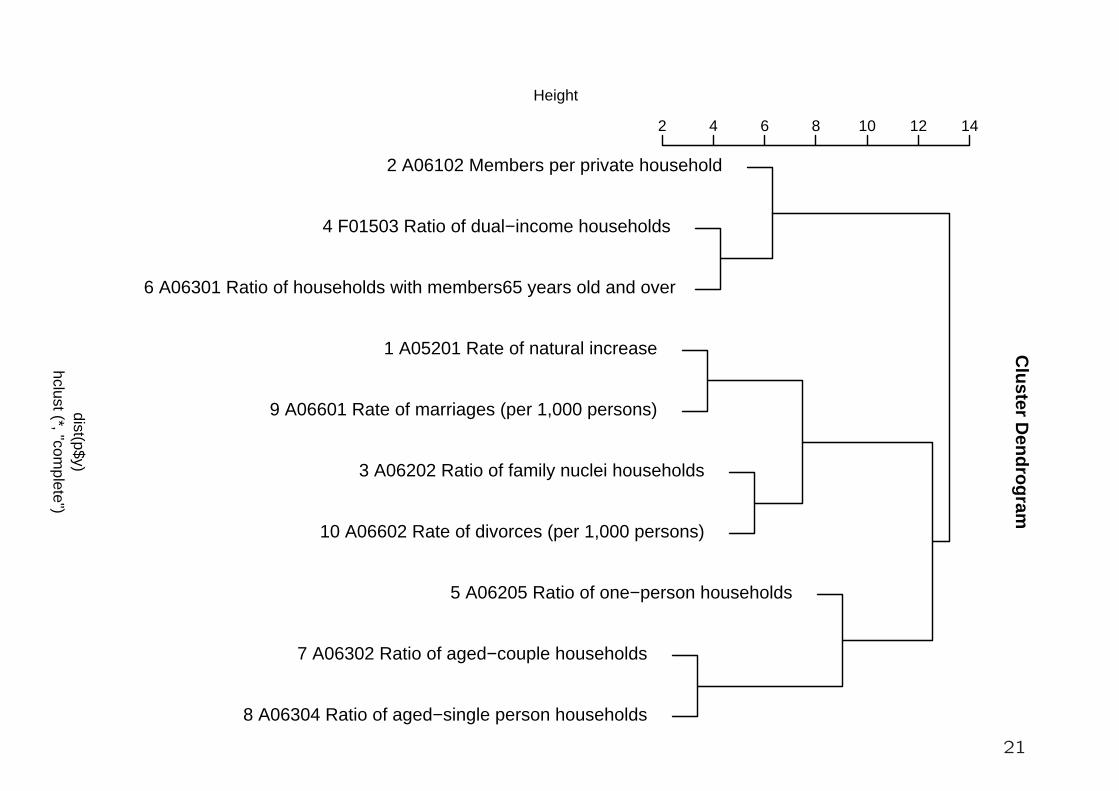
> hy <- hclust(dist(p$y))
> # show clustering
> plot(hx,cex=1.2)
> plot(hy,labels=na,cex=0.9)
> # show matrix
> image(seq(along=hx$order),seq(along=hy$order),
+ scale(x)[hx$order,rev(hy$order)],
+ col=heat.colors(60),axes=F,xlab="",ylab="")
> axis(1,seq(along=hx$order),rownames(p$x)[hx$order],las=2)
> axis(2,seq(along=hy$order),rownames(p$y)[rev(hy$order)],las=2)
19

Aom
ori
Oka
yam
aK
agaw
aT
okus
him
aK
umam
oto
Ishi
kaw
aN
agan
oG
ifuG
umm
aY
aman
ashi
Mie A
kita
Shi
man
eIw
ate
Niig
ata
Tot
tori
Fuk
ushi
ma
Sag
aY
amag
ata
Toy
ama
Fuk
uiO
kina
wa
Kan
agaw
aO
saka M
iyag
iS
higa
Ibar
aki
Toc
higi
Shi
zuok
aN
ara
Aic
hiS
aita
ma
Chi
baT
okyo
Hok
kaid
oF
ukuo
kaH
yogo
Kyo
toH
irosh
ima
Wak
ayam
aN
agas
aki
Miy
azak
iO
oita
Yam
aguc
hiE
him
eK
ochi
Kag
oshi
ma
02
46
810
Cluster Dendrogram
hclust (*, "complete")dist(p$x)
Hei
ght
20
2 A06102 Members per private household
4 F01503 Ratio of dual−income households
6 A06301 Ratio of households with members65 years old and over
1 A05201 Rate of natural increase
9 A06601 Rate of marriages (per 1,000 persons)
3 A06202 Ratio of family nuclei households
10 A06602 Rate of divorces (per 1,000 persons)
5 A06205 Ratio of one−person households
7 A06302 Ratio of aged−couple households
8 A06304 Ratio of aged−single person households
2 4 6 8 10 12 14
Clu
ster Den
dro
gram
hclust (*, "complete")
dist(p$y)
Height
21

Aom
ori
Oka
yam
aK
agaw
aT
okus
him
aK
umam
oto
Ishi
kaw
aN
agan
oG
ifuG
umm
aY
aman
ashi
Mie
Aki
taS
him
ane
Iwat
eN
iigat
aT
otto
riF
ukus
him
aS
aga
Yam
agat
aT
oyam
aF
ukui
Oki
naw
aK
anag
awa
Osa
kaM
iyag
iS
higa
Ibar
aki
Toc
higi
Shi
zuok
aN
ara
Aic
hiS
aita
ma
Chi
baT
okyo
Hok
kaid
oF
ukuo
kaH
yogo
Kyo
toH
irosh
ima
Wak
ayam
aN
agas
aki
Miy
azak
iO
oita
Yam
aguc
hiE
him
eK
ochi
Kag
oshi
ma
A06304
A06302
A06205
A06602
A06202
A06601
A05201
A06301
F01503
A06102
22

Aom
ori
Oka
yam
aK
agaw
aT
okus
him
aK
umam
oto
Ishi
kaw
aN
agan
oG
ifuG
umm
aY
aman
ashi
Mie A
kita
Shi
man
eIw
ate
Niig
ata
Tot
tori
Fuk
ushi
ma
Sag
aY
amag
ata
Toy
ama
Fuk
uiO
kina
wa
Kan
agaw
aO
saka M
iyag
iS
higa
Ibar
aki
Toc
higi
Shi
zuok
aN
ara
Aic
hiS
aita
ma
Chi
baT
okyo
Hok
kaid
oF
ukuo
kaH
yogo
Kyo
toH
irosh
ima
Wak
ayam
aN
agas
aki
Miy
azak
iO
oita
Yam
aguc
hiE
him
eK
ochi
Kag
oshi
ma
02
46
810
Cluster Dendrogram
hclust (*, "complete")dist(p$x)
Hei
ght
Aom
ori
Oka
yam
aK
agaw
aT
okus
him
aK
umam
oto
Ishi
kaw
aN
agan
oG
ifuG
umm
aY
aman
ashi
Mie
Aki
taS
him
ane
Iwat
eN
iigat
aT
otto
riF
ukus
him
aS
aga
Yam
agat
aT
oyam
aF
ukui
Oki
naw
aK
anag
awa
Osa
kaM
iyag
iS
higa
Ibar
aki
Toc
higi
Shi
zuok
aN
ara
Aic
hiS
aita
ma
Chi
baT
okyo
Hok
kaid
oF
ukuo
kaH
yogo
Kyo
toH
irosh
ima
Wak
ayam
aN
agas
aki
Miy
azak
iO
oita
Yam
aguc
hiE
him
eK
ochi
Kag
oshi
ma
A06304
A06302
A06205
A06602
A06202
A06601
A05201
A06301
F01503
A061022 A06102 Members per private household
4 F01503 Ratio of dual−income households
6 A06301 Ratio of households with members65 years old and over
1 A05201 Rate of natural increase
9 A06601 Rate of marriages (per 1,000 persons)
3 A06202 Ratio of family nuclei households
10 A06602 Rate of divorces (per 1,000 persons)
5 A06205 Ratio of one−person households
7 A06302 Ratio of aged−couple households
8 A06304 Ratio of aged−single person households
2 4 6 8 10 12 14
Clu
ster Den
dro
gram
hclust (*, "complete")
dist(p$y)
Height
23

回帰分析
• データ解析で最も利用頻度の高い分析法• 重回帰 = multiple regression
• 従属変数yと独立変数x1, x2, . . . , xmの関係を推定
y = β0 + β1x1 + β2x2 + · · · + βmxm + ε
• 係数βiが yとxiの関係を表す
24
重回帰分析の関数
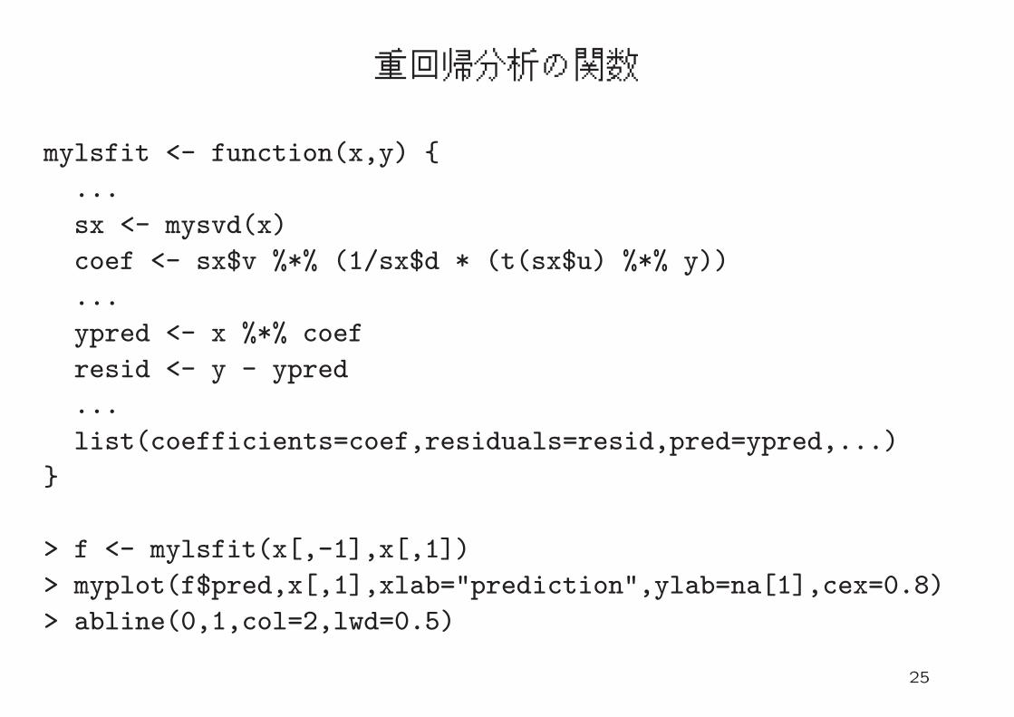
mylsfit <- function(x,y) {
...
sx <- mysvd(x)
coef <- sx$v %*% (1/sx$d * (t(sx$u) %*% y))
...
ypred <- x %*% coef
resid <- y - ypred
...
list(coefficients=coef,residuals=resid,pred=ypred,...)
}
> f <- mylsfit(x[,-1],x[,1])
> myplot(f$pred,x[,1],xlab="prediction",ylab=na[1],cex=0.8)
> abline(0,1,col=2,lwd=0.5)
25

−0.2 0.0 0.2 0.4 0.6
−0.
20.
00.
20.
40.
6
prediction
1 A
0520
1 R
ate
of n
atur
al in
crea
se
Hokkaido
Aomori
Iwate
Miyagi
Akita
Yamagata
Fukushima
IbarakiTochigiGumma
Saitama
Chiba
Tokyo
Kanagawa
NiigataToyama
IshikawaFukui
YamanashiNagano
GifuShizuoka
Aichi
Mie
Shiga
Kyoto
Osaka
Hyogo
Nara
WakayamaTottori
Shimane
Okayama
Hiroshima
Yamaguchi
Tokushima
Kagawa
Ehime
Kochi
Fukuoka
Saga
NagasakiKumamoto
Ooita
Miyazaki
Kagoshima
Okinawa
26

> round(f$tsummary,3)
, , = Y
Estimate Std.Err t-value Pr(>|t|)
Intercept -7.887 1.334 -5.913 0.000
A06102 1.691 0.192 8.808 0.000
A06202 0.024 0.010 2.553 0.015
F01503 0.003 0.003 0.978 0.334
A06205 0.056 0.013 4.359 0.000
A06301 -0.022 0.009 -2.335 0.025
A06302 0.051 0.017 2.992 0.005
A06304 -0.010 0.016 -0.599 0.553
A06601 0.107 0.027 3.984 0.000
A06602 0.108 0.043 2.521 0.016
27

サンプルセッション2
> ### randomly selecting items
> a0 <- X2000$code[grep("^.$",X2000$clab)] # indices
> a0
[1] "A01101" "A01601" "A0160101" "A0160102" "A0160103" "A01201"
[7] "A01202" "A01302" "A01401" "A01402" "A02101" "A02102"
[13] "A02103" "A02104" "A03101" "A03102" "A03103" "A03401"
[19] "A03402" "A03403" "A03404" "A0410301" "A0410302" "A0410401"
[25] "A0410402" "A0410501" "A0410502" "A0410601" "A0410602" "A0410701"
[31] "A0410702" "A0410801" "A0410802" "A0430701" "A0430702" "A0440501"
[37] "A0440502" "A0440601" "A0440602" "A05101" "A05201" "A05202"
[43] "A05203" "A05204" "A0520401" "A0520402" "A05205" "A05218"
[49] "A0521901" "A0521902" "A05301" "A05302" "A05303" "A05304"
[55] "A05305" "A0610101" "A06102" "A06202" "F01503" "A06205"
[61] "A06301" "A06302" "A06304" "A06601" "A06602" "B01101"
[67] "B01202" "B01205" "B01204" "B01301" "B01401" "B0140101"
[73] "B0140102" "B0140103" "B02101" "B02102" "B02103" "B02201"
[79] "B02401" "B02402" "B02301" "B02303" "B02304" "C01301"28

[85] "C01101" "C01105" "C01106" "C01107" "C02102" "C02103"
[91] "C02201" "C02205" "C03201" "C03205" "C03303" "C0330303"
[97] "C03304" "C0330408" "C0410101" "C04105" "C04106" "C0410701"
[103] "C04401" "C04404" "C04505" "C04507" "C04601" "C0460101"
[109] "C04602" "L04201" "L04203" "L04101" "L04102" "L04104"
[115] "L04105" "L04106" "L04107" "L04108" "L04109" "L04110"
[121] "L04111" "L04112" "L04113" "L04302" "L04304" "D0110101"
[127] "D01102" "D0120101" "D0130201" "D01401" "D0140201" "D0140301"
[133] "D0210101" "D0210201" "D0210301" "D0220103" "D02202" "D02204"
[139] "D02206" "D02207" "D0310301" "D0310401" "D0310501" "D0310601"
[145] "D0310701" "D0310801" "D0310901" "D0311001" "D0311101" "D0311201"
[151] "D03113" "D03114" "D0311501" "D0312301" "D0320101" "D0320201"
[157] "D0320301" "D0330103" "D0330203" "D0330303" "D0330403" "D0330503"
[163] "D0330603" "D0330703" "D0331103" "D03312" "D03313" "D0331403"
[169] "D0332003" "D0332103" "D0331503" "D0331603" "D0331703" "D0331803"
[175] "D0331903" "E0110101" "E0110102" "E0110103" "E0110104" "E0110105"
[181] "E0110201" "E0110202" "E0110203" "E01303" "E01304" "E01305"
[187] "E0210101" "E0210102" "E0210103" "E02601" "E02602" "E02603"
[193] "E02701" "E02702" "E02703" "E0410201" "E0410202" "E0510301"

[199] "E0510302" "E0510303" "E0510304" "E0510305" "E05203" "E05204"
[205] "E05205" "E0610101" "E0610102" "E0610201" "E0610202" "E0620401"
[211] "E0620402" "E0620403" "E08101" "E08102" "E08201" "E08202"
[217] "E0910101" "E0910102" "E0910402" "E09211" "E09212" "I0821101"
[223] "I0821102" "E09213" "E09214" "E09401" "E09402" "E0940302"
[229] "E09501" "E09502" "E09503" "E09504" "F0110101" "F0110102"
[235] "F01201" "F01202" "F01203" "F01301" "F0130101" "F0130102"
[241] "F02301" "F02501" "F0260101" "F02701" "F02702" "F03101"
[247] "F03102" "F03103" "F03104" "F0320101" "F03303" "F03302"
[253] "F03301" "F03304" "F03401" "F03403" "F03402" "F0350101"
[259] "F0350201" "F03601" "F03602" "F04101" "F04102" "F04103"
[265] "F04104" "F05101" "F0610101" "F0610102" "F0620101" "F0620102"
[271] "F06204" "F0620301" "F0620302" "F0620303" "F0620304" "G01101"
[277] "G01104" "G01107" "G01109" "G01115" "G01202" "G01311"
[283] "G01313" "G01314" "G01315" "G01316" "G01317" "G03201"
[289] "G03203" "G0320501" "G03207" "G04101" "G04211" "G04306"
[295] "G04307" "G05102" "G0430501" "H01301" "H01302" "H0130202"
[301] "H01204" "H01601" "H01603" "H01401" "H01402" "H01403"
[307] "H02104" "H0210301" "H0210302" "H0210701" "H0210703" "H02101"

[313] "H0210101" "H0210102" "H0220301" "H0220302" "H0210201" "H0210202"
[319] "H02302" "H02303" "H02601" "H04101" "H04102" "H04301"
[325] "H05102" "H05201" "H05304" "H05306" "H0540101" "H05503"
[331] "H05504" "H05601" "H06101" "H06103" "H06105" "H06107"
[337] "H06109" "H06111" "H06113" "H0611302" "H06125" "H06117"
[343] "H06119" "H06121" "H06302" "H06309" "H06305" "H06306"
[349] "H06307" "H06401" "H06402" "H06406" "H06408" "H06412"
[355] "H06501" "H0650101" "H0650102" "H03101" "H07201" "H0720202"
[361] "H0720201" "H0720204" "H0720203" "H0720205" "H0720206" "H08101"
[367] "H08301" "H08302" "H08303" "H08304" "I04105" "I04104"
[373] "I04102" "I04103" "I0420102" "I0420103" "I0420202" "I0420203"
[379] "I05101" "I0520101" "I0520102" "I0520201" "I0520202" "I0520501"
[385] "I0520502" "I06101" "I06102" "I06103" "I06104" "I06105"
[391] "I06106" "I06201" "I07101" "I07102" "I07103" "I07104"
[397] "I07105" "I07201" "I0210101" "I0210102" "I0210103" "I0210104"
[403] "I0210105" "I0210106" "I0210201" "I0210202" "I0210203" "I0210204"
[409] "I0210205" "I0210206" "I0910103" "I0910105" "I0910106" "I0910107"
[415] "I0910203" "I0910205" "I0920101" "I0920201" "I0920301" "I0930201"
[421] "I0930301" "I09401" "I09402" "I0950102" "I0950103" "I0950104"

[427] "I10101" "I10102" "I10103" "I10104" "I10105" "I10201"
[433] "I10202" "I10203" "I10204" "I10205" "I11101" "I11102"
[439] "I11201" "I12201" "I13102" "I13207" "I13201" "I13402"
[445] "I14101" "I14102" "I14201" "I14202" "J01101" "J01107"
[451] "J0110803" "J0110804" "J0110902" "J01200" "J02101" "J02201"
[457] "J02204" "J02202" "J02203" "J02301" "J02401" "J02501"
[463] "J03101" "J03201" "J03202" "J03203" "J03301" "J03401"
[469] "J03501" "J04101" "J04102" "J04201" "J04202" "J04203"
[475] "J04204" "J04301" "J04302" "J04401" "J04402" "J05101"
[481] "J05102" "J05103" "J05107" "J05201" "J05202" "J05203"
[487] "J05206" "J05204" "J05207" "J0610101" "J0610102" "I15101"
[493] "I15102" "I15103" "I15202" "I1520301" "I1520302" "I1520401"
[499] "I1520402" "F07101" "F07102" "F08101" "F08102" "F08201"
[505] "F08202" "K01102" "K01104" "K01105" "K01107" "K01301"
[511] "K01302" "K01401" "K01402" "K02101" "K02103" "K02203"
[517] "K02205" "K02301" "K02303" "K02306" "K03102" "K03104"
[523] "K03112" "K04102" "K04101" "K04105" "K04106" "K04107"
[529] "K04201" "K04202" "K04301" "K05102" "K05103" "K06101"
[535] "K06104" "K06201" "K06204" "K06401" "K06402" "K06403"

[541] "K06405" "K06301" "K06304" "K06501" "K06503" "K07105"
[547] "K08101" "K09201" "K10101" "K10105" "K10107" "K10201"
[553] "K10203" "K10301" "K10304" "K10305" "K10401" "K10403"
[559] "K10501" "K10502" "K10503" "L01201" "L01204" "L02602"
[565] "L02201" "L02401" "L02402" "L02403" "L02404" "L02405"
[571] "L02406" "L02407" "L02408" "L02409" "L02410" "L02734"
[577] "L02735" "L02736" "L01100" "L0110101" "L0110102" "L02601"
[583] "L02101" "L02301" "L03201" "L03212" "L03213" "L03214"
[589] "L03401" "L03412" "L03602" "L03603" "L03604" "L03606"
[595] "L03607" "M01101" "M01102" "M0120106" "M0120206" "M0120107"
[601] "M0120207" "M0130106" "M0130206" "M0130107" "M0130207" "M0210101"
[607] "M0210201" "M0310101" "M0310201" "M0310102" "M0310202" "M0330101"
[613] "M0330201" "M0330102" "M0330202"
> a <- sample(a0,10) # randomly select 10 items
> a
[1] "I07104" "K06401" "E0610202" "F07102" "E09502" "D03113"
[7] "L01100" "J02301" "D0331803" "I0950103"
> a <- sample(a0,10) # randomly select 10 items again
> a

[1] "J05107" "H05102" "K07105" "C02201" "D0311001" "L04201"
[7] "A0430701" "H06117" "H08303" "M0210201"
> na <- paste(seq(along=a),a,X2000$item[a])
> na
[1] "1 J05107 Homehelpers(per 100,000 persons) "
[2] "2 H05102 Ratio of households coveredby city gas supply system "
[3] "3 K07105 Value of damage by disasters(per capita) "
[4] "4 C02201 Ratio of private establishmentswith 1-4 persons "
[5] "5 D0311001 Ratio of agriculture, forestryand fishery expenditure [prefe
[6] "6 L04201 Regional difference index of consumerprices [general : ku-area
[7] "7 A0430701 Ratio of widowed population[60 years old and over, male] "
[8] "8 H06117 Barbers and beauty shops(per 100,000 persons) "
[9] "9 H08303 Neighborhood parksper inhabitable area 100k "
[10] "10 M0210201 Work [female with a job] "
> jna <- paste(seq(along=a),a,X2000$jitem[a])
> jna
[1] "1 J05107 訪問介護員(ホームヘルパー)数(人口10万人当たり) "
[2] "2 H05102 都市ガス供給区域内世帯比率 "
[3] "3 K07105 災 害 被 害 額(人口1人当たり) "

[4] "4 C02201 従業者1~4人の事業所割合[民 営] "
[5] "5 D0311001 農 林 水 産 業 費 割 合[県財政] "
[6] "6 L04201 消費者物価地域差指数[総合:東京都区部=100] "
[7] "7 A0430701 死 別 者 割 合[60歳以上・男] "
[8] "8 H06117 理 容 ・ 美 容 所 数(人口10万人当たり) "
[9] "9 H08303 近 隣 公 園 数(可住地面積100k�当たり) "
[10] "10 M0210201 仕 事 の 平 均 時 間[有業者・女] "
> x <- X2000$x[,a]
> dim(x)
[1] 47 10
>

−0.2 0.0 0.2 0.4
−0.
20.
00.
20.
4
PC 1
PC
2
−6 −4 −2 0 2 4 6 8
−6
−4
−2
02
46
8
1 J05107 Homehelpers(pe
2 H05102
3 K07105 Value of damage by disasters(per capita)
4 C02201 Ratio of private establishmentswith 1−4 persons
5 D0311001 Ratio of agriculture, forestryand fishery expenditure [prefecture6 L04201 Regi
7 A0430701 Ratio of widowed population[60 years old and over, ma
8 H06117 Barbers and beauty shops(per 100,000 persons)
9 H08303 N
10 M0210201 Work [female with a job]
Hokkaido
Aomori
Iwate
Miyagi
Akita
Yamagata
Fukushima
Ibaraki
TochigiGumma
SaitamaChiba
Tok
Kanag
NiigataToyama
Ishikawa
Fukui
Yamanashi
Nagano
Gifu
Shizuoka
Aichi
MieShiga
Kyoto
Osaka
HyogoNaraWakayama
Tottori
Shimane
Okayama
Hiroshima
Yamaguchi
Tokushima
Kagawa
Ehime
Kochi
Fukuoka
Saga
Nagasaki
Kumamoto
Ooita
MiyazakiKagoshima
Okinawa
29
−0.3 −0.2 −0.1 0.0 0.1 0.2 0.3
−0.
3−
0.2
−0.
10.
00.
10.
20.
3
PC 3
PC
2
−4 −2 0 2
−4
−2
02
1
2
3
4
5
6
7
8
9
10
Hokkaido
Aomori
Iwate
Miyagi
Akita
Yamagata
Fukushima
Ibaraki
TochigiGumma
SaitamaChiba
Tokyo
Kanagawa
Niigata
Toyama
Ishikawa
Fukui
Yamanashi
Nagano
Gifu
Shizuoka
Aichi
Mie
Shiga
Kyoto
Osaka
HyogoNaraWakayama
Tottori
Shimane
Okayama
Hiroshima
Yamaguchi
Tokushima
Kagawa
Ehime
Kochi
Fukuoka
Saga
Nagasaki
umamoto
Ooita
MiyazakiKagoshima
Okinawa
30

Tok
yoK
anag
awa
Osa
kaS
aita
ma
Chi
baA
ichi
Hyo
goN
iigat
aH
okka
ido
Miy
agi
Hiro
shim
aY
amag
uchi
Toy
ama
Ishi
kaw
aS
higa
Mie
Oka
yam
aK
yoto
Nar
aS
hizu
oka
Fuk
uoka
Kag
awa
Fuk
ushi
ma
Tot
tori
Gum
ma
Ibar
aki
Toc
higi
Tok
ushi
ma
Yam
anas
hiW
akay
ama
Iwat
eK
umam
oto
Gifu
Koc
hiO
kina
wa
Fuk
uiN
agas
aki
Shi
man
eK
agos
him
aN
agan
oS
aga
Ooi
taE
him
eM
iyaz
aki A
omor
iA
kita
Yam
agat
a
02
46
810
Cluster Dendrogram
hclust (*, "complete")dist(p$x)
Hei
ght
31

1 J05107 Homehelpers(per 100,000 persons)
6 L04201 Regional difference index of consumerprices [general : ku−area of Tokyo = 100]
2 H05102 Ratio of households coveredby city gas supply system
9 H08303 Neighborhood parksper inhabitable area 100k
3 K07105 Value of damage by disasters(per capita)
7 A0430701 Ratio of widowed population[60 years old and over, male]
4 C02201 Ratio of private establishmentswith 1−4 persons
8 H06117 Barbers and beauty shops(per 100,000 persons)
5 D0311001 Ratio of agriculture, forestryand fishery expenditure [prefecture]
10 M0210201 Work [female with a job]
4 6 8 12
Clu
ster Den
dro
gram
hclust (*, "complete")
dist(p$y)
Height
32

Tok
yoK
anag
awa
Osa
kaS
aita
ma
Chi
baA
ichi
Hyo
goN
iigat
aH
okka
ido
Miy
agi
Hiro
shim
aY
amag
uchi
Toy
ama
Ishi
kaw
aS
higa Mie
Oka
yam
aK
yoto
Nar
aS
hizu
oka
Fuk
uoka
Kag
awa
Fuk
ushi
ma
Tot
tori
Gum
ma
Ibar
aki
Toc
higi
Tok
ushi
ma
Yam
anas
hiW
akay
ama
Iwat
eK
umam
oto
Gifu
Koc
hiO
kina
wa
Fuk
uiN
agas
aki
Shi
man
eK
agos
him
aN
agan
oS
aga
Ooi
taE
him
eM
iyaz
aki
Aom
ori
Aki
taY
amag
ata
M0210201
D0311001
H06117
C02201
A0430701
K07105
H08303
H05102
L04201
J05107
33

Tok
yoK
anag
awa
Osa
kaS
aita
ma
Chi
baA
ichi
Hyo
goN
iigat
aH
okka
ido
Miy
agi
Hiro
shim
aY
amag
uchi
Toy
ama
Ishi
kaw
aS
higa
Mie
Oka
yam
aK
yoto
Nar
aS
hizu
oka
Fuk
uoka
Kag
awa
Fuk
ushi
ma
Tot
tori
Gum
ma
Ibar
aki
Toc
higi
Tok
ushi
ma
Yam
anas
hiW
akay
ama
Iwat
eK
umam
oto
Gifu
Koc
hiO
kina
wa
Fuk
uiN
agas
aki
Shi
man
eK
agos
him
aN
agan
oS
aga
Ooi
taE
him
eM
iyaz
aki A
omor
iA
kita
Yam
agat
a
02
46
810
Cluster Dendrogram
hclust (*, "complete")dist(p$x)
Hei
ght
Tok
yoK
anag
awa
Osa
kaS
aita
ma
Chi
baA
ichi
Hyo
goN
iigat
aH
okka
ido
Miy
agi
Hiro
shim
aY
amag
uchi
Toy
ama
Ishi
kaw
aS
higa Mie
Oka
yam
aK
yoto
Nar
aS
hizu
oka
Fuk
uoka
Kag
awa
Fuk
ushi
ma
Tot
tori
Gum
ma
Ibar
aki
Toc
higi
Tok
ushi
ma
Yam
anas
hiW
akay
ama
Iwat
eK
umam
oto
Gifu
Koc
hiO
kina
wa
Fuk
uiN
agas
aki
Shi
man
eK
agos
him
aN
agan
oS
aga
Ooi
taE
him
eM
iyaz
aki
Aom
ori
Aki
taY
amag
ata
M0210201
D0311001
H06117
C02201
A0430701
K07105
H08303
H05102
L04201
J051071 J05107 Homehelpers(per 100,000 persons)
6 L04201 Regional difference index of consumerprices [general : ku−area of Tokyo = 100]
2 H05102 Ratio of households coveredby city gas supply system
9 H08303 Neighborhood parksper inhabitable area 100k
3 K07105 Value of damage by disasters(per capita)
7 A0430701 Ratio of widowed population[60 years old and over, male]
4 C02201 Ratio of private establishmentswith 1−4 persons
8 H06117 Barbers and beauty shops(per 100,000 persons)
5 D0311001 Ratio of agriculture, forestryand fishery expenditure [prefecture]
10 M0210201 Work [female with a job]
4 6 8 12
Clu
ster Den
dro
gram
hclust (*, "complete")
dist(p$y)
Height
34

100 150 200
5010
015
020
025
030
0
prediction
1 J0
5107
Hom
ehel
pers
(per
100
,000
per
sons
)
HokkaidoAomori
IwateMiyagiAkitaYamagata
Fukushima
Ibaraki
TochigiGumma
SaitamaChiba
Tokyo
Kanagawa
Niigata
Toyama
Ishikawa
Fukui
Yamanashi
Nagano
GifuShizuoka
Aichi
Mie
Shiga
Kyoto
Osaka
Hyogo
Nara
WakayamaTottori
Shimane
Okayama HiroshimaYamaguchi
Tokushima
Kagawa
Ehime
Kochi
Fukuoka
Saga
Nagasaki
Kumamoto
OoitaMiyazaki Kagoshima
Okinawa
35

> round(f$tsummary,3)
, , = Y
Estimate Std.Err t-value Pr(>|t|)
Intercept -1092.573 522.218 -2.092 0.043
H05102 0.458 0.600 0.764 0.450
K07105 0.001 0.000 1.259 0.216
C02201 4.757 3.484 1.365 0.180
D0311001 0.411 2.963 0.139 0.891
L04201 5.493 4.361 1.259 0.216
A0430701 6.486 13.400 0.484 0.631
H06117 -0.048 0.170 -0.283 0.778
H08303 7.267 2.901 2.505 0.017
M0210201 53.139 40.318 1.318 0.196
36

サンプルセッション3
> ### values
> ## character, numeric, and NA types
> "hello"
[1] "hello"
> 123/456
[1] 0.2697368
> sqrt(3/4)
[1] 0.8660254
> sin(pi/3)
[1] 0.8660254
> 1==2
[1] FALSE
> 1==1
[1] TRUE
> 1/0 # infinity
[1] Inf
> sqrt(-1) # not a number37

[1] NaN
Warning message:
NaNs produced in: sqrt(-1)
> sin(NA) # not available
[1] NA
> ## vector
> c(1,3,2,4)
[1] 1 3 2 4
> 10:20
[1] 10 11 12 13 14 15 16 17 18 19 20
> 30:20
[1] 30 29 28 27 26 25 24 23 22 21 20
> seq(0,10,0.1) # sequence from 0 to 10 increasing by 0.1
[1] 0.0 0.1 0.2 0.3 0.4 0.5 0.6 0.7 0.8 0.9 1.0 1.1 1.2 1.3
[16] 1.5 1.6 1.7 1.8 1.9 2.0 2.1 2.2 2.3 2.4 2.5 2.6 2.7 2.8
[31] 3.0 3.1 3.2 3.3 3.4 3.5 3.6 3.7 3.8 3.9 4.0 4.1 4.2 4.3
[46] 4.5 4.6 4.7 4.8 4.9 5.0 5.1 5.2 5.3 5.4 5.5 5.6 5.7 5.8
[61] 6.0 6.1 6.2 6.3 6.4 6.5 6.6 6.7 6.8 6.9 7.0 7.1 7.2 7.3
[76] 7.5 7.6 7.7 7.8 7.9 8.0 8.1 8.2 8.3 8.4 8.5 8.6 8.7 8.8

[91] 9.0 9.1 9.2 9.3 9.4 9.5 9.6 9.7 9.8 9.9 10.0
> a <- 10:20
> length(a) # length of vector
[1] 11
> seq(along=a)
[1] 1 2 3 4 5 6 7 8 9 10 11
> seq(from=1,to=length(a))
[1] 1 2 3 4 5 6 7 8 9 10 11
> 1:length(a)
[1] 1 2 3 4 5 6 7 8 9 10 11
> help(seq) # show the help message for the function "seq"
> rep(3,10) # replicate elements
[1] 3 3 3 3 3 3 3 3 3 3
> rep(c(3,4),c(10,20))
[1] 3 3 3 3 3 3 3 3 3 3 4 4 4 4 4 4 4 4 4 4 4 4 4 4 4 4 4 4 4 4
> rep(abc,1:4)
[1] "abc" "def" "def" "ghi" "ghi" "ghi" "hello" "hello" "hello"
[10] "hello"
> help(rep)

> ### variables
> ## simple assignment
> a <- 1
> a
[1] 1
> a <- 1:10
> a
[1] 1 2 3 4 5 6 7 8 9 10
> a^2
[1] 1 4 9 16 25 36 49 64 81 100
> b <- a*a
> b
[1] 1 4 9 16 25 36 49 64 81 100

> plot(a,b)
2 4 6 8 10
020
4060
8010
0
a
b
38

> plot(a,sqrt(a))
2 4 6 8 10
1.0
1.5
2.0
2.5
3.0
a
sqrt
(a)
39

> a <- seq(0,10,0.1)
> plot(a,sqrt(a))
> plot(a,sqrt(a),type="l")
40

> plot(a,sqrt(a))
0 2 4 6 8 10
0.0
0.5
1.0
1.5
2.0
2.5
3.0
a
sqrt
(a)
41
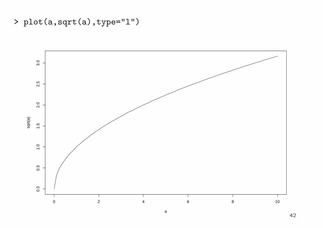
> plot(a,sqrt(a),type="l")
0 2 4 6 8 10
0.0
0.5
1.0
1.5
2.0
2.5
3.0
a
sqrt
(a)
42

> abc <- c("abc","def","ghi","hello")
> abc
[1] "abc" "def" "ghi" "hello"
> ## output postscript file
> options(papersize="a4")
> a <- 1:10
> b <- a*a
> postscript("ex01pt1.eps")
> plot(a,b)
> dev.off()
X11
2
> postscript("ex01pt2.eps")
> plot(a,sqrt(a))
> dev.off()
X11
2
> a <- seq(0,10,0.1)
> plot(a,sqrt(a))43
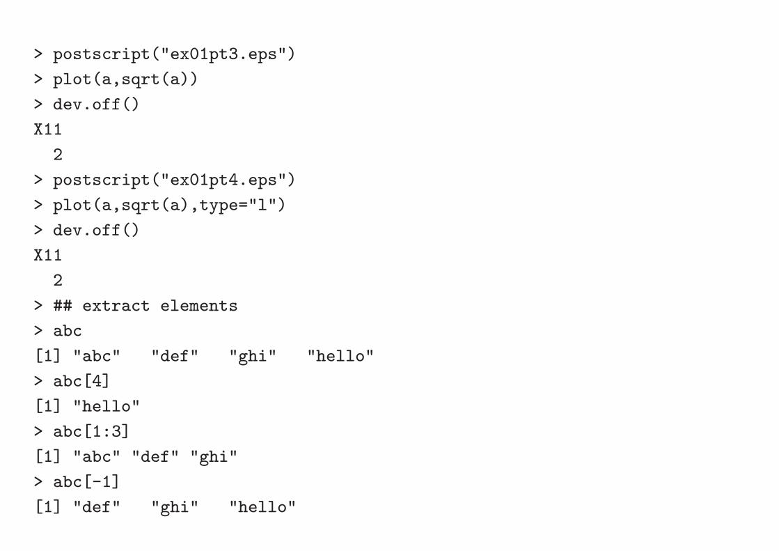
> postscript("ex01pt3.eps")
> plot(a,sqrt(a))
> dev.off()
X11
2
> postscript("ex01pt4.eps")
> plot(a,sqrt(a),type="l")
> dev.off()
X11
2
> ## extract elements
> abc
[1] "abc" "def" "ghi" "hello"
> abc[4]
[1] "hello"
> abc[1:3]
[1] "abc" "def" "ghi"
> abc[-1]
[1] "def" "ghi" "hello"

> abc[5]
[1] NA
> a <- 101:110
> a
[1] 101 102 103 104 105 106 107 108 109 110
> a[1]
[1] 101
> a[10]
[1] 110
> a[11]
[1] NA
> a[-1]
[1] 102 103 104 105 106 107 108 109 110
> a[-(1:5)]
[1] 106 107 108 109 110
> a %% 2 # modulo by 2
[1] 1 0 1 0 1 0 1 0 1 0
> a %% 2 == 0 # even numbers
[1] FALSE TRUE FALSE TRUE FALSE TRUE FALSE TRUE FALSE TRUE

> a[ a%%2==0 ]
[1] 102 104 106 108 110
> a[ a%%2==1 ]
[1] 101 103 105 107 109
> a >= 105
[1] FALSE FALSE FALSE FALSE TRUE TRUE TRUE TRUE TRUE TRUE
> a[ a>=105 ]
[1] 105 106 107 108 109 110
> ## matrix
> a <- matrix(1:6,3,2) # matrix of size 3 x 2 with elements 1:6
> a
[,1] [,2]
[1,] 1 4
[2,] 2 5
[3,] 3 6
> dim(a) # dimensions
[1] 3 2
> t(a) # matrix transpose
[,1] [,2] [,3]

[1,] 1 2 3
[2,] 4 5 6
> t(a) %*% a # multiplication
[,1] [,2]
[1,] 14 32
[2,] 32 77
> a %*% t(a)
[,1] [,2] [,3]
[1,] 17 22 27
[2,] 22 29 36
[3,] 27 36 45
> a <- matrix(1:4,2,2) # matrix of size 2 x 2 with elements 1:4
> a
[,1] [,2]
[1,] 1 3
[2,] 2 4
> b <- solve(a) # inverse matrix
> b
[,1] [,2]

[1,] -2 1.5
[2,] 1 -0.5
> a %*% b # should be identity matrix
[,1] [,2]
[1,] 1.000000e+00 -5.551115e-17
[2,] 4.440892e-16 1.000000e-00
> round(a%*%b, 6) # show results with 6 digits
[,1] [,2]
[1,] 1 0
[2,] 0 1
> b %*% a
[,1] [,2]
[1,] 1 4.440892e-16
[2,] 0 1.000000e-00
> a * a # element-wize multiplication
[,1] [,2]
[1,] 1 9
[2,] 4 16
> a %*% a # matrix multiplication

[,1] [,2]
[1,] 7 15
[2,] 10 22
> sin(a) # element-wise sin()
[,1] [,2]
[1,] 0.8414710 0.1411200
[2,] 0.9092974 -0.7568025
> a %% 2 == 0
[,1] [,2]
[1,] FALSE FALSE
[2,] TRUE TRUE
> a[a %% 2 == 0] # result becomes a vector
[1] 2 4
> ## more on matrix
> a <- matrix(1:20,4) # matrix of size 4 x 5
> a
[,1] [,2] [,3] [,4] [,5]
[1,] 1 5 9 13 17
[2,] 2 6 10 14 18

[3,] 3 7 11 15 19
[4,] 4 8 12 16 20
> a[3,] # the third row
[1] 3 7 11 15 19
> a[,3] # the third column
[1] 9 10 11 12
> a[2:3,] # the second and third rows
[,1] [,2] [,3] [,4] [,5]
[1,] 2 6 10 14 18
[2,] 3 7 11 15 19
> a[,2:3] # the second and third columns
[,1] [,2]
[1,] 5 9
[2,] 6 10
[3,] 7 11
[4,] 8 12
> a[3,,drop=F] # the third row as matrix
[,1] [,2] [,3] [,4] [,5]
[1,] 3 7 11 15 19

> a[,3,drop=F] # the third column as matrix
[,1]
[1,] 9
[2,] 10
[3,] 11
[4,] 12
> ### names and dimnames
> ## vector
> a <- 10:15
> a
[1] 10 11 12 13 14 15
> names(a) <- c("ten","eleven","twelve","thirteen","fourteen","fifteen")
> a
ten eleven twelve thirteen fourteen fifteen
10 11 12 13 14 15
> names(a)
[1] "ten" "eleven" "twelve" "thirteen" "fourteen" "fifteen"
> a[2]
eleven
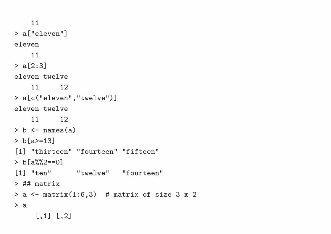
11
> a["eleven"]
eleven
11
> a[2:3]
eleven twelve
11 12
> a[c("eleven","twelve")]
eleven twelve
11 12
> b <- names(a)
> b[a>=13]
[1] "thirteen" "fourteen" "fifteen"
> b[a%%2==0]
[1] "ten" "twelve" "fourteen"
> ## matrix
> a <- matrix(1:6,3) # matrix of size 3 x 2
> a
[,1] [,2]

[1,] 1 4
[2,] 2 5
[3,] 3 6
> rownames(a) <- c("one","two","three")
> a
[,1] [,2]
one 1 4
two 2 5
three 3 6
> colnames(a) <- c("ichi","ni")
> a
ichi ni
one 1 4
two 2 5
three 3 6
> rownames(a)
[1] "one" "two" "three"
> colnames(a)
[1] "ichi" "ni"
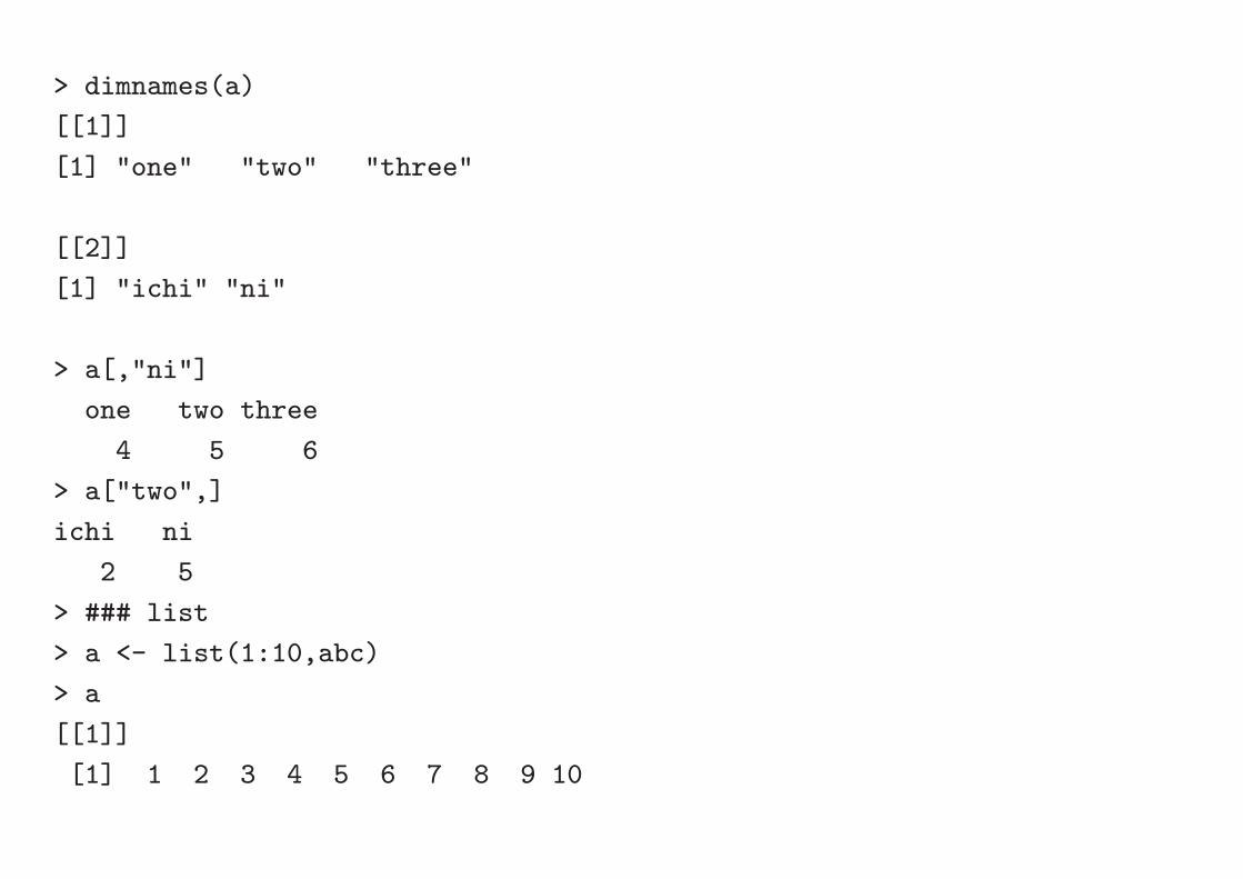
> dimnames(a)
[[1]]
[1] "one" "two" "three"
[[2]]
[1] "ichi" "ni"
> a[,"ni"]
one two three
4 5 6
> a["two",]
ichi ni
2 5
> ### list
> a <- list(1:10,abc)
> a
[[1]]
[1] 1 2 3 4 5 6 7 8 9 10
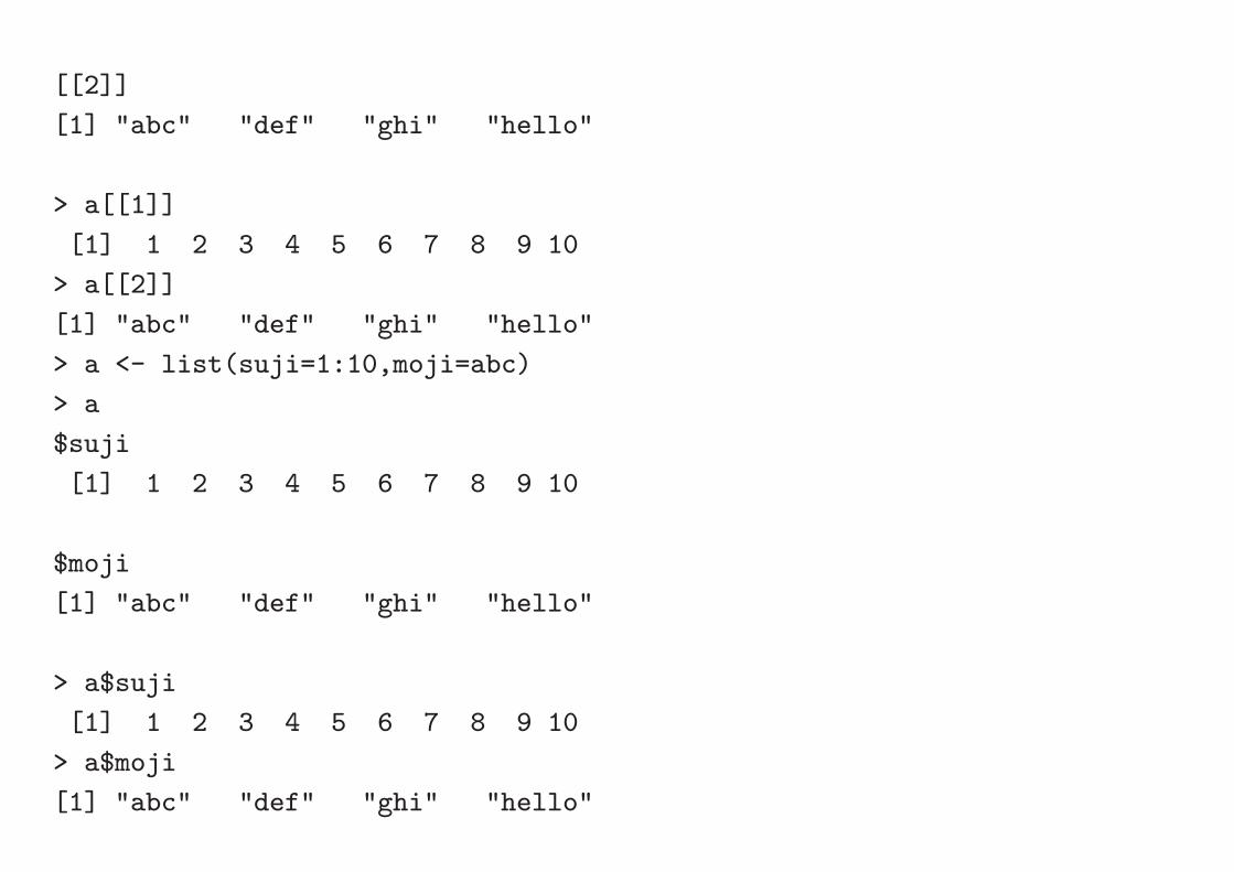
[[2]]
[1] "abc" "def" "ghi" "hello"
> a[[1]]
[1] 1 2 3 4 5 6 7 8 9 10
> a[[2]]
[1] "abc" "def" "ghi" "hello"
> a <- list(suji=1:10,moji=abc)
> a
$suji
[1] 1 2 3 4 5 6 7 8 9 10
$moji
[1] "abc" "def" "ghi" "hello"
> a$suji
[1] 1 2 3 4 5 6 7 8 9 10
> a$moji
[1] "abc" "def" "ghi" "hello"

> ### simple analysis
> ## load a sample dataset
> source("~shimo/class/gakubu200209/data20020919c.R")
> x
jinkou souseisan
Hokkaido 5683062 197473
Aomori 1475728 45620
Iwate 1416180 46949
Miyagi 2365320 86155
Akita 1189279 38414
Yamagata 1244147 41119
Fukushima 2126935 78345
Ibaraki 2985676 110819
Tochigi 2004817 79962
Gumma 2024852 77960
Saitama 6938006 199636
Chiba 5926285 183721
Tokyo 12064101 846809
Kanagawa 8489974 298661
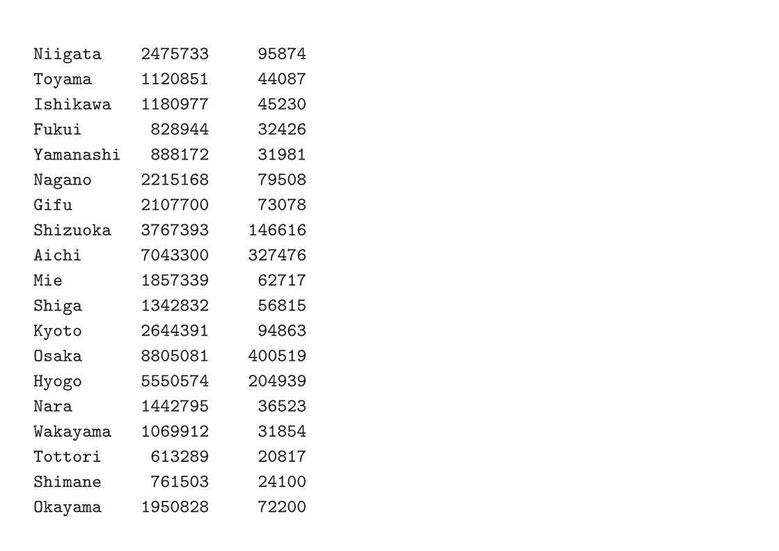
Niigata 2475733 95874
Toyama 1120851 44087
Ishikawa 1180977 45230
Fukui 828944 32426
Yamanashi 888172 31981
Nagano 2215168 79508
Gifu 2107700 73078
Shizuoka 3767393 146616
Aichi 7043300 327476
Mie 1857339 62717
Shiga 1342832 56815
Kyoto 2644391 94863
Osaka 8805081 400519
Hyogo 5550574 204939
Nara 1442795 36523
Wakayama 1069912 31854
Tottori 613289 20817
Shimane 761503 24100
Okayama 1950828 72200

Hiroshima 2878915 110162
Yamaguchi 1527964 55796
Tokushima 824108 26357
Kagawa 1022890 38295
Ehime 1493092 48146
Kochi 813949 23417
Fukuoka 5015699 169834
Saga 876654 28484
Nagasaki 1516523 46426
Kumamoto 1859344 57580
Ooita 1221140 42965
Miyazaki 1170007 34026
Kagoshima 1786194 51166
Okinawa 1318220 34249
> x["Tokyo",]
jinkou souseisan
12064101 846809
> x[,"jinkou"]
Hokkaido Aomori Iwate Miyagi Akita Yamagata Fukushima Ibara

5683062 1475728 1416180 2365320 1189279 1244147 2126935 29856
Tochigi Gumma Saitama Chiba Tokyo Kanagawa Niigata Toya
2004817 2024852 6938006 5926285 12064101 8489974 2475733 11208
Ishikawa Fukui Yamanashi Nagano Gifu Shizuoka Aichi M
1180977 828944 888172 2215168 2107700 3767393 7043300 18573
Shiga Kyoto Osaka Hyogo Nara Wakayama Tottori Shima
1342832 2644391 8805081 5550574 1442795 1069912 613289 7615
Okayama Hiroshima Yamaguchi Tokushima Kagawa Ehime Kochi Fukuo
1950828 2878915 1527964 824108 1022890 1493092 813949 50156
Saga Nagasaki Kumamoto Ooita Miyazaki Kagoshima Okinawa
876654 1516523 1859344 1221140 1170007 1786194 1318220
> ## plot and fitting
> plot(x) # simple plot

2.0e+06 4.0e+06 6.0e+06 8.0e+06 1.0e+07 1.2e+07
0e+
002e
+05
4e+
056e
+05
8e+
05
jinkou
sous
eisa
n
44

> plot(x,type="n") # draw only frame
> text(x,rownames(x)) # draw labels
> f <- lsfit(x[,1],x[,2]) # least square fitting (kaiki-bunseki)
> abline(f) # draw a fitted line
45

2.0e+06 4.0e+06 6.0e+06 8.0e+06 1.0e+07 1.2e+07
0e+
002e
+05
4e+
056e
+05
8e+
05
jinkou
sous
eisa
n
Hokkaido
AomoriIwate
Miyagi
AkitaYamagataFukushima
IbarakiTochigiGumma
SaitamaChiba
Tokyo
Kanagawa
Niigata
ToyamaIshikawaFukuiYamanashi
NaganoGifu
Shizuoka
Aichi
MieShiga
Kyoto
Osaka
Hyogo
NaraWakayamaTottoriShimane
OkayamaHiroshima
YamaguchiTokushima
KagawaEhimeKochi
Fukuoka
SagaNagasakiKumamoto
OoitaMiyazakiKagoshima
Okinawa
46
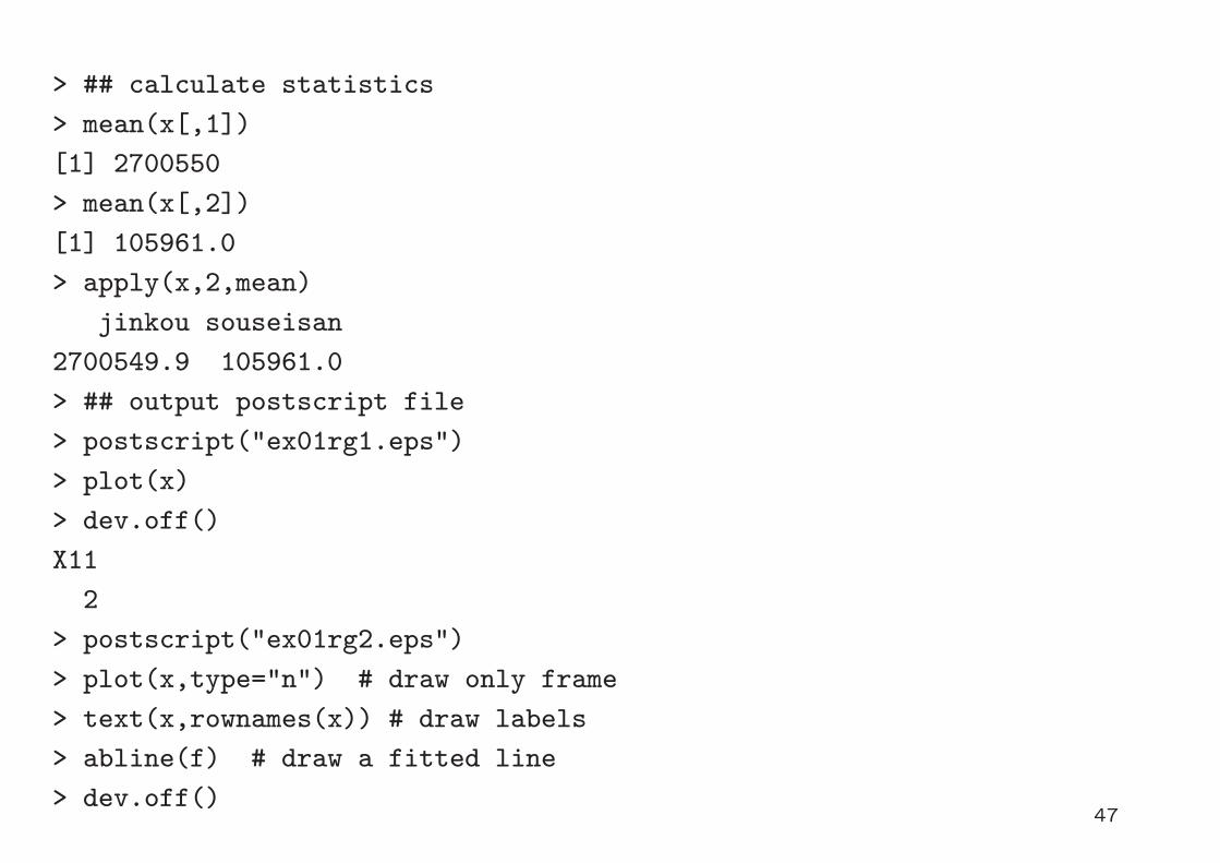
> ## calculate statistics
> mean(x[,1])
[1] 2700550
> mean(x[,2])
[1] 105961.0
> apply(x,2,mean)
jinkou souseisan
2700549.9 105961.0
> ## output postscript file
> postscript("ex01rg1.eps")
> plot(x)
> dev.off()
X11
2
> postscript("ex01rg2.eps")
> plot(x,type="n") # draw only frame
> text(x,rownames(x)) # draw labels
> abline(f) # draw a fitted line
> dev.off()47
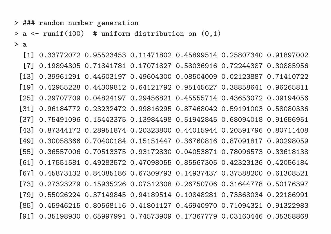
> ### random number generation
> a <- runif(100) # uniform distribution on (0,1)
> a
[1] 0.33772072 0.95523453 0.11471802 0.45899514 0.25807340 0.91897002
[7] 0.19894305 0.71841781 0.17071827 0.58036916 0.72244387 0.30885956
[13] 0.39961291 0.44603197 0.49604300 0.08504009 0.02123887 0.71410722
[19] 0.42955228 0.44309812 0.64121792 0.95145627 0.38858641 0.96265811
[25] 0.29707709 0.04824197 0.29456821 0.45555714 0.43653072 0.09194056
[31] 0.96184772 0.23232472 0.99816295 0.87468042 0.59191003 0.58080336
[37] 0.75491096 0.15443375 0.13984498 0.51942845 0.68094018 0.91656951
[43] 0.87344172 0.28951874 0.20323800 0.44015944 0.20591796 0.80711408
[49] 0.30058366 0.70400184 0.15151447 0.36760816 0.87091817 0.90298059
[55] 0.36557006 0.70513375 0.93172830 0.04053871 0.78096573 0.33618138
[61] 0.17551581 0.49283572 0.47098055 0.85567305 0.42323136 0.42056184
[67] 0.45873132 0.84085186 0.67309793 0.14937437 0.37588200 0.61308521
[73] 0.27323279 0.15935226 0.07312308 0.26750706 0.31644778 0.50176397
[79] 0.55026224 0.37149845 0.94189514 0.10848281 0.73368034 0.22186991
[85] 0.45946215 0.80568116 0.41801127 0.46940970 0.71094321 0.91322983
[91] 0.35198930 0.65997991 0.74573909 0.17367779 0.03160446 0.35358868

[97] 0.39337573 0.75346727 0.02309114 0.91162517
> hist(a)
> a <- runif(1000)
> hist(a)
> a <- runif(10000)
> mean(a)
[1] 0.5010653
> var(a)
[1] 0.08278935
> a <- runif(10000)
> mean(a)
[1] 0.4979175
> var(a)
[1] 0.08332883
> hist(a)
> abline(h=500)
> postscript("ex01unif.eps")
> hist(a)
> abline(h=500)

> dev.off()
X11
2

Histogram of a
a
Fre
quen
cy
0.0 0.2 0.4 0.6 0.8 1.0
010
020
030
040
050
0
48

> a <- rnorm(100) # normal distribution with mean 0 and varianc 1
> a
[1] -0.82691765 -2.02067099 0.19400892 -0.30382863 -0.31811388 -0.77346330
[7] -0.40153550 2.41079419 0.60562417 -0.97393404 -1.23733634 0.85196384
[13] -0.60534823 -0.77889770 -0.07444445 2.66534621 -0.83451795 0.45235685
[19] -0.10990285 1.08580316 -0.74960909 0.40406038 0.60829232 1.45375506
[25] 0.75997487 -1.20344286 -0.85792115 -0.15464927 0.15831217 0.08548434
[31] 0.50799391 -1.80017291 0.88274744 -1.15015568 0.01921664 2.05726484
[37] 0.37508515 -0.49540912 -0.92401419 0.38382362 0.27878916 -1.00021783
[43] -0.63664893 0.69261984 -0.32744108 0.01033082 -0.50170459 1.24632212
[49] 1.52279633 -0.49338017 0.68571754 -0.70039005 -0.25592276 -1.85568359
[55] 0.99690176 0.98597080 0.51932234 2.18836775 0.12552985 0.46521986
[61] -1.33403257 -0.89277524 1.32653428 -0.35091993 -0.37484179 0.40620331
[67] 1.42748708 0.65026413 0.42211847 1.34728761 -0.30578058 0.53137451
[73] 0.15892649 -0.35528093 1.53916414 1.65100974 0.70355433 0.56355801
[79] -0.24340207 -0.44164793 0.73611704 1.18361392 -0.87211264 1.08447142
[85] -0.57204720 1.17112253 -0.50147376 -0.32345874 2.00594036 0.68166394
[91] -0.65396266 0.24280340 0.89660829 -0.19244041 0.91239919 0.13789878
[97] -1.45605476 -1.66931721 -0.66200807 -2.3246790049

> hist(a)
> a <- rnorm(1000)
> hist(a)
> a <- rnorm(10000)
> hist(a)
> mean(a)
[1] -0.005828347
> var(a)
[1] 0.992512
> b <- seq(-4,4,length=100)
> lines(b,dnorm(b)*0.5*10000)
> postscript("ex01norm.eps")
> hist(a)
> lines(b,dnorm(b)*0.5*10000)
> dev.off()
X11
2

Histogram of a
a
Fre
quen
cy
−4 −2 0 2 4
050
010
0015
0020
00
50

> ### function
> foo <- function(x) x*x
> foo
function(x) x*x
> foo(5)
[1] 25
> foo(1:10)
[1] 1 4 9 16 25 36 49 64 81 100
> goo <- function(x,y) x*y
> goo(3,5)
[1] 15
> goo(1:10,2)
[1] 2 4 6 8 10 12 14 16 18 20
> goo <- function(x,y=2) x*y
> goo(1:10,2)
[1] 2 4 6 8 10 12 14 16 18 20
> goo(1:10)
[1] 2 4 6 8 10 12 14 16 18 20
> foo <- function(x) { # dont type the following "+" prompt marks51
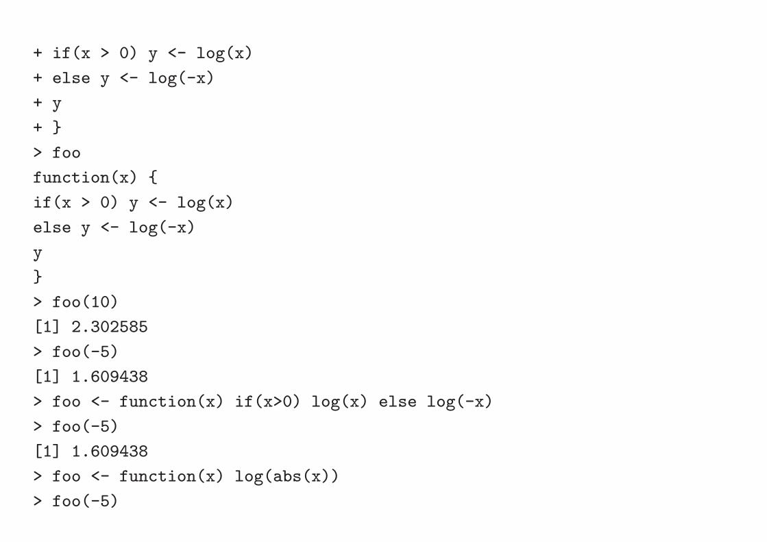
+ if(x > 0) y <- log(x)
+ else y <- log(-x)
+ y
+ }
> foo
function(x) {
if(x > 0) y <- log(x)
else y <- log(-x)
y
}
> foo(10)
[1] 2.302585
> foo(-5)
[1] 1.609438
> foo <- function(x) if(x>0) log(x) else log(-x)
> foo(-5)
[1] 1.609438
> foo <- function(x) log(abs(x))
> foo(-5)

[1] 1.609438
> ## end
> q()
Save workspace image? [y/n/c]: y
Process R finished at Fri Sep 20 00:47:40 2002