


Languages
Pages
Legal


Sep 6 ISMT 162/Stuart Zhu 1
Lecture 2: Time Series Forecasting
• Forecasting and production• Data and demand patterns• Stationary demand forecasting model• Naïve method• Moving average method• Exponential smoothing method• Summary• Readings: Page 68-87

Sep 6 ISMT 162/Stuart Zhu 2
Forecasting and Production• Business planning is based
on forecast (and strategy)– Is this new product going to
sale?
– What is the potential market for this new product?
– Will customer accept this new technology?
– How much to produce in each period?
– Availability of raw materials?
– Changes in interest rates, exchange rates, material prices?
• Bad forecasts are costly– Sony’s video technology,
Apple computer (customer/tech)
– IBM’s notebooks (new product sales potential)
– Stock-out and markdown can cost more than manufacturing cost (Fisher et al. 1994)

Sep 6 ISMT 162/Stuart Zhu 3
Making and Using Forecasts • Forecasts are usually made by marketing and sales• Forecasts are decision inputs for marketing and
production/operations• Forecasting horizon in operation planning
– short term product sales forecast in days or weeks for inventory management and production plan (MRP)
– intermediate term forecast of sales patterns in weeks or months of product family for labor and resource requirement
– long term demand trend forecast in months or years for capacity planning

Sep 6 ISMT 162/Stuart Zhu 4
Steps in the Forecasting Process
Step 1 Determine purpose of forecast
Step 2 Establish a time horizon
Step 3 Select a forecasting technique
Step 4 Obtain, clean and analyze data
Step 5 Make the forecast
Step 6 Monitor the forecast
“The forecast”

Sep 6 ISMT 162/Stuart Zhu 5
Subjective Forecasting Methods
• Sales force composites– sales manager aggregates
salesmen’s individual sales estimates
– could be biased
• Consumer survey (market research)– for signals of future trend
and shift of preference patterns,
– survey and sampling design needs specialist
• Executive opinion– no data, expert opinion is
the only source of information
– interview or consensus meeting
• The Delphi method– formal and iterative method
of coming up a forecast from
– experts’ opinion, a group of experts and a facilitator

Sep 6 ISMT 162/Stuart Zhu 6
Sport Obermeyer, an Example6 managers look at the new styles and estimate sales (short life-cycle products)
ForecastsMember Pandora Parka Entice JacketCarolyn 1,200 1,500Laura 1,150 700Tom 1,250 1,200Kenny 1,300 300Wally 1,100 2,075Wendy 1,200 1,425Average
Std. Dev1,20070.7
1,200627.1

Sep 6 ISMT 162/Stuart Zhu 7
Objective Forecasting Methods
• Time Series models– past data contains future demand information and
can be used to project future demands– used for operation planning
• Associative models– uses explanatory variables to predict the future

Sep 6 ISMT 162/Stuart Zhu 8
Data and Demand Patterns
Data Analysis
• We need to know the demand pattern before selecting an appropriate forecasting model
• How?
• Plot the data to examine the pattern– Example data sets:
forecast-s1– Also Figure 3.1 (P. 73)
• What are the common patterns?
• Why is it important to determine the pattern first?

Sep 6 ISMT 162/Stuart Zhu 9
Demand Patterns
t tA a
t tA a bt
t t tA ac
( )t t tA a bt c
Stationary/constant
Linear trend
Cyclic/seasonal
Cyclic/seasonal with trend
forecast-s1
εt : a random fluctuation; a, b: constant;
ct : time-varying coefficient
Sep 6 ISMT 162/Stuart Zhu 10
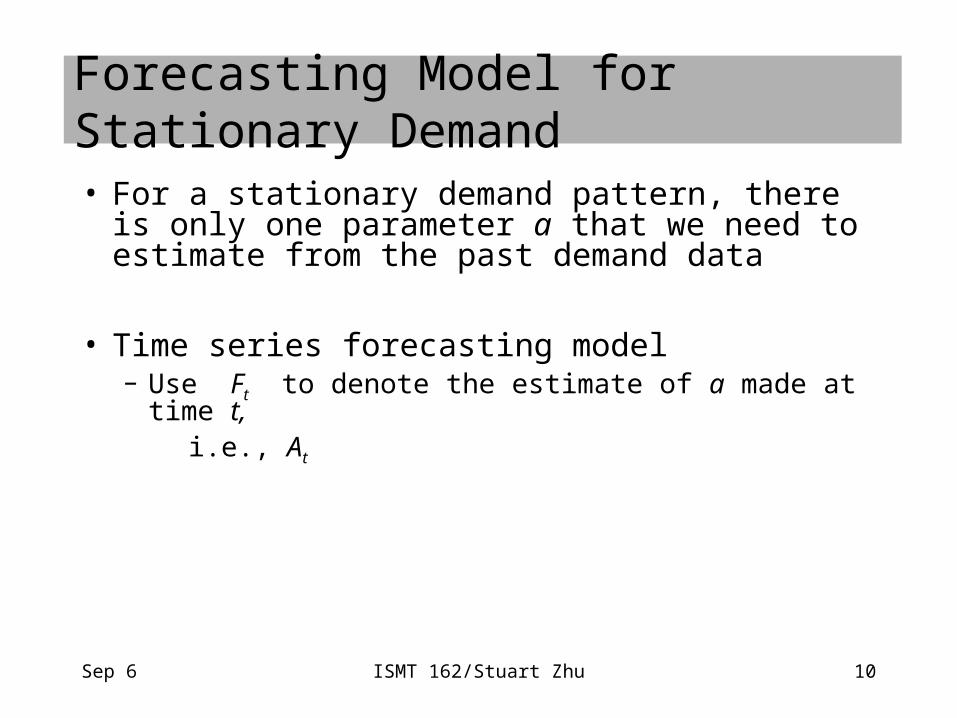
Forecasting Model for Stationary Demand
• For a stationary demand pattern, there is only one parameter a that we need to estimate from the past demand data
• Time series forecasting model– Use Ft to denote the estimate of a made at time t, i.e., At

Sep 6 ISMT 162/Stuart Zhu 11
Time Series Forecasting
Methods to obtain Ft
• Naïve • N-period moving
average• Exponential
smoothing
• Purpose:– To estimate the
parameters of the demand model, using past data
– To filter out the random element from the past data
Sep 6 ISMT 162/Stuart Zhu 12
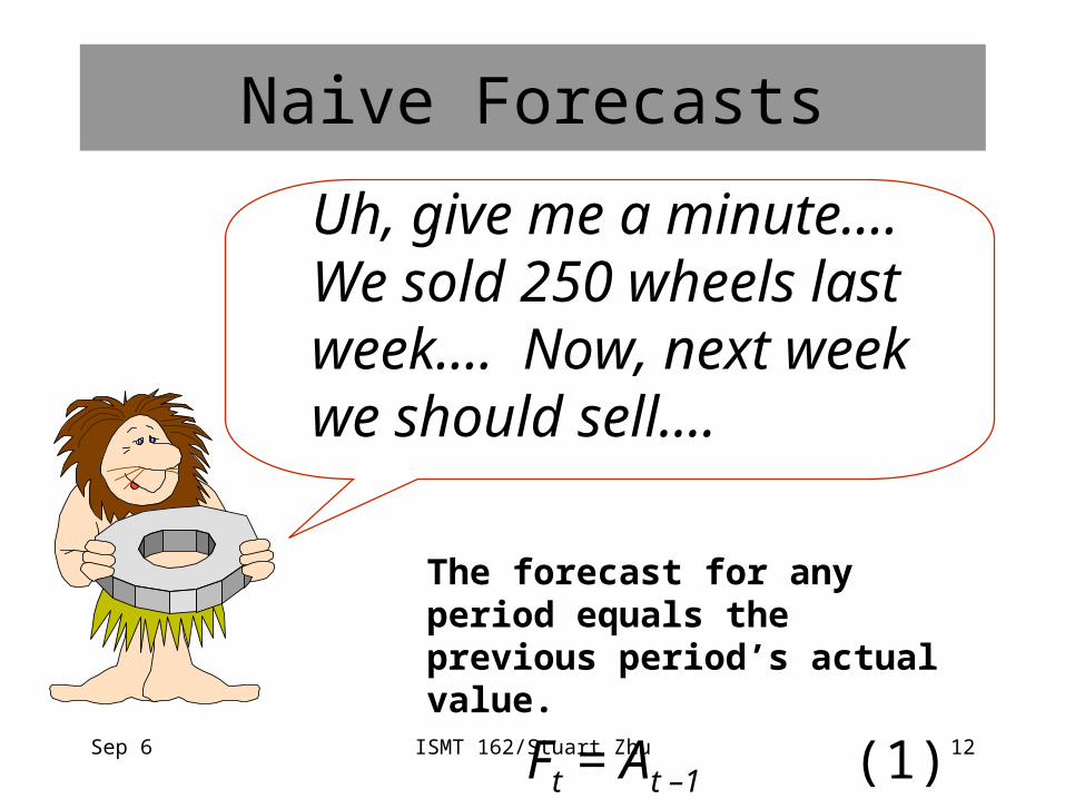
Naive Forecasts
Uh, give me a minute.... We sold 250 wheels lastweek.... Now, next week we should sell....
The forecast for any period equals the previous period’s actual value.
Ft = At –1 (1)

Sep 6 ISMT 162/Stuart Zhu 13
• Simple to use
• Virtually no cost
• Quick and easy to prepare
• Data analysis is nonexistent
• Easily understandable
• Cannot provide high accuracy
• Can be a standard for accuracy
Naïve Forecasts

Sep 6 ISMT 162/Stuart Zhu 14
N-Period Moving Average
• Select only the recent data
• Example 1 Passed demand data: 106 110 118 105 115 100 112 106 118 102 112 110
• What is the forecast for period 13? Or for period 15?
• With N =3
• With N =5
• Choice of N: ≥3 • forecast-s2
1
1 n
t t ii
F An
(2)

Sep 6 ISMT 162/Stuart Zhu 15
Exponential Smoothing
• Use Ft to denote the estimate of a at period t,
is the smoothing constant
• Data: 106 110 118 105 115 100 112 106 118 102 112 110
• What is the forecast for period 13?
forecast-s2
1 1 1
1 1
( )
(1 )t t t t
t t
F F A F
A F
(3)
Sep 6 ISMT 162/Stuart Zhu 16
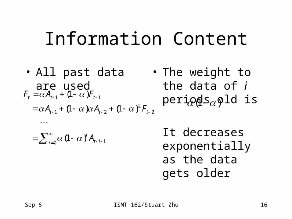
Information Content
• All past data are used • The weight to the data of i periods old is
It decreases exponentially as the data gets older
1 1
21 2 2
10
(1 )
(1 ) (1 )
(1 )
t t t
t t t
it ii
F A F
A A F
A
(1 )i

Sep 6 ISMT 162/Stuart Zhu 17
Choice of Smoothing Constant • Between 0 and 1 (why?)• If the demand is stable, choose a small ; if the
demand is rapidly increasing or decreasing, choose a large . (why?)– determines the weight on the most recent data
• We should test the forecast model to fit a good • Usually is from 0.1 to 0.3

Sep 6 ISMT 162/Stuart Zhu 18
Summary
• Distinguish three things in time series forecast:– the underlying process
– parameter estimation
– and forecasting formula/model
• Equations (1), (2), (3)
• Keys to good forecast– Good data
– Right model
– Proper balance of forecasting stability and sensitivity to the recent change in data, through selection of N and

Sep 6 ISMT 162/Stuart Zhu 19
Forecast Variations
Trend
Irregularvariation
Seasonal variations
908988
Cycles

Sep 6 ISMT 162/Stuart Zhu 20
Review Problems
• Problem 1 at page 112
• Problem 3 at page 113
• Problem 4 at page 113

Sep 6 ISMT 162/Stuart Zhu 21
A Caveat on Forecasts
• “Man won’t fly for 1000 years”Wilbur Wright - 1901
• “No woman in my time will be Prime Minister”Margaret Thatcher – 1969
• “I think there is a world market for about five computers”
Thomas J. Watson - 1958
Top Related