

![16 Solidification 051117 [호환 모드]ocw.snu.ac.kr/sites/default/files/NOTE/9_Solidification... · 2018. 4. 17. · 1. Solidification of single-phase alloys 1) Equilibrium Solidification:](https://static.fdocument.pub/doc/165x107/60a9f070a0dd125f6c752d2c/16-solidification-051117-eeoeocwsnuackrsitesdefaultfilesnote9solidification.jpg)


Languages
Pages
Legal

Dissertation DI Johann Peter Mogeritsch
Investigation on Peritectic Solidification
using a Transparent Organic System
A thesis submitted to the University of Leoben
for the degree of Doctor of montanistische Wissenschaften
Presented by
Johann P. Mogeritsch
Leoben, June 2012
Examiner: Univ.-Prof. Dipl.-Phys. Dr.rer.nat. Andreas Ludwig
Chair for Simulation and Modelling of Metallurgical Processes
Department of Metallurgy
Co-Examiner: Univ.-Prof. Dipl.-Ing. Dr.phil. Peter Schumacher
Chair of Casting Research
Department of Metallurgy
I
Eidesstattliche Erklärung
Ich erkläre an Eides statt, dass ich diese Arbeit selbstständig verfasst, andere als die
angegebenen Quellen und Hilfsmittel nicht benützt und mich auch sonst keiner unerlaubten
Hilfsmittel bedient habe.
Leoben, 25.06.2012
DI Johann Peter Mogeritsch

II
Affidavit
I declare in lieu of oath, that I wrote this thesis and performed the associated research myself,
using only literature cited in this volume.
Leoben, 25.06.2012
DI Johann Peter Mogeritsch

III
Danksagung
Mit Dank möchte ich all die Hilfe und Unterstützung wertschätzen, die mir während der
Erstellung meiner Doktorarbeit von meiner Familie, meinen Betreuern und Arbeitskollegen
zuteil wurde. Besonders möchte ich meiner Lebensgefährtin Jacqueline danken, die mir
immer mit ihrer Unterstützung und vor allem auch mit Ihrer Geduld zur Seite stand.
Speziell möchte ich mich bei Herrn Prof. Andreas Ludwig, dem Hauptbetreuer meiner
Dissertation und meinem Chef am Lehrstuhl für Modellierung und Simulation metallurgischer
Prozesse für die Möglichkeit der Verfassung der Dissertation danken. Seine fachliche
Kompetenz, konstruktive Kritik aber auch Motivation haben in vielen Gespräche und
Diskussionen sehr zum Gelingen dieser Doktorarbeit beigetragen. Vielen Dank auch Herrn
Prof. Peter Schumacher als Zweitbetreuer der Doktorarbeit und seine Unterstützung durch
experimentellen Messungen.
Viel Arbeit hatten auch meine beiden Betreuer, Frau Dr. Monika Grasser und Herr Dr. Sven
Eck, denen ich für Ihre Unterstützung recht herzlich danke.
Mein Dank gilt aber auch der ESA und ASA die gemeinsam die Finanzierung der Dissertation
ermöglicht haben und meinen Projektkollegen von METCOMP und DIRSOL.
Ich möchte aber auch meinen Arbeitskollegen für die gute und freundschaftliche
Zusammenarbeit danken. Speziell sei hier auch das Sekretariat und die die EDV Abteilung
erwähnt, denn ohne sie wäre diese Arbeit nicht möglich gewesen.

1
Abstract
In the last decades the importance of metals and metallic alloys underlies an increasing
importance, and with it the requirements on properties and quality of alloys. Important
commercial alloys are for example steel, aluminum, copper, tin, and zinc alloys. Due to the
fact that they show peritectic reactions in the phase diagram, it is of great importance to
improve the understanding of a peritectic reaction and related morphologies leading to
improved material properties of high quality. In the last century great efforts were made to
gain deeper understanding of the microstructure formation in peritectic alloys during
solidification, especially in cases where both phases solidify as a planar front.
The formation of a microstructure from the melt is influenced by convection in front of the
solid/liquid interface, a consequence of the existing gravity on earth. Without gravity the
natural convection does not operate, such as in the orbiting International Space Station (ISS).
Therefore, the European Space Agency (ESA) supports investigations on peritectic
solidification morphologies within the frame of the project “Metastable Solidification of
Composites” (METCOMP).
To estimate the influence of natural convection on solidification morphologies the
investigations within this project were divided into ground experiments, under normal gravity,
and space experiments, under micro gravity. Due to a delay of the construction of the
Bridgman-furnace for in-situ observation of direct solidification (DIRSOL) in space by ESA,
the experiments in space had to be postponed to 2014. Thus the influence of the natural
convection on the solidification morphologies remains to be elucidated in detail.
Investigations on peritectic metallic systems show a wide range of possible microstructures.
Bands, tree-like microstructures, islands, and coupled growth were detected at a growth rate
where both phases can solidify in form of a planar front. To improve the understanding of
appearing morphologies during solidification transparent model systems for in-situ
observation are an attractive option. Such systems offer the advantage that both, the
morphology and the dynamics of solidification can be investigated by using optical diagnostic
means. The organic phase diagram TRIS - NPG was selected for this study because
temperature and concentration of the peritectic point are suitable for direct observation in a
micro Bridgman-furnace setup. The organic compound TRIS is used for in-situ observation
for the first time. Therefore, additional investigations to complete the physical properties of

2
TRIS and the alloys of TRIS - NPG had to be performed. Whereby, thermal instability of the
organic compound TRIS was detected that constrains the processing window for in-situ
observations.
The investigations on the organic phase diagram TRIS – NPG indicated a wide range of
microstructures, whereby, well known structures as well as ones were found close to the limit
of constitutional undercooling at the peritectic region. Oscillating behavior was found close to
the peritectic concentration at pulling rates above the limit of constitutional undercooling.
Here, both phases grow in a competitive manner in a way that oscillating solidification occurs.
This kind of solidification was observed for the first time and no literature has been found up
to now that describes this behavior. At a solidification rate close and below the limit of
constitutional undercooling only a planar solidification front was found. In a few cases the
growth of isothermal peritectic coupled growth (PCG) or banded growth which lead to
isothermal PCG was observed. Evidence for this form of transformation were found in
experiments with metals and supported with numerical simulation. Here, it was the first time
that the transformation from banded to PCG is reported by direct observation.
3
Contents
1 Introduction ........................................................................................................................... 5
2 State of the Art ...................................................................................................................... 8 2.1 Peritectic Solidification ............................................................................................... 8
2.1.1 Solidification Rate above the Critical Solidification Velocity Vc,
Cells and Dendrites .......................................................................................... 14 2.1.2 Solidification Rate below the Critical Solidification Velocity Vc,
Layered Structures ........................................................................................... 15 2.2 Organic Compounds ................................................................................................. 20
2.2.1 Organic Compound NPG .................................................................................. 22 2.2.2 Organic Compound TRIS ................................................................................. 22
2.2.3 Phase Diagram TRIS - NPG ............................................................................. 24 3 Experimental Methods ........................................................................................................ 27
3.1 Sample Preparation ................................................................................................... 27 3.1.1 Alloy Preparation .............................................................................................. 28
3.1.2 Sample Geometry ............................................................................................. 29 3.1.3 Sample Filling ................................................................................................... 29
3.2 Differential Scanning Calorimetry (DSC) ................................................................ 30 3.3 Bridgman Components ............................................................................................. 31
3.3.1 Micro Bridgman-furnace set up ........................................................................ 32 3.3.2 Optical Observation System “DIoS” ................................................................ 34
4 Stability and Reproducibility of the NPG – TRIS System ................................................. 36 4.1 Phase Diagram of TRIS – NPG ................................................................................ 36
4.2 Available Physical and Chemical Properties of TRIS and NPG .............................. 41 4.3 Investigation on the Organic Material ...................................................................... 42
4.3.1 Material Purification ......................................................................................... 42 4.3.2 Reproducibility of the Alloy Concentration ..................................................... 42 4.3.3 Thermal Stability .............................................................................................. 46
4.4 Corresponding Consequences ................................................................................... 50 4.4.1 Conclusions from the Thermal Stability Investigation ..................................... 50
4.4.2 Selection of Optimal Process Conditions ......................................................... 51 4.5 Selected Experimental Procedure ............................................................................. 54
4.5.1 Experimental Type A: Unmoved Samples ....................................................... 55 4.5.2 Experimental Type B: Moved Samples ............................................................ 55
5 Results ................................................................................................................................. 56
5.1 Experimental Type A: Unmoved Samples ................................................................ 56 5.1.1 Samples with pure TRIS ................................................................................... 56 5.1.2 Samples with pure NPG.................................................................................... 59 5.1.3 Samples with Selected Concentrations ............................................................. 60
5.2 Experimental Type B: Moved Samples .................................................................... 63 5.2.1 Preparation of the Solid/Liquid Interface ......................................................... 63 5.2.2 Solidification Morphologies in the [Cl] and the [CF] Phase Region ................. 64 5.2.3 Layered Structure Morphologies ...................................................................... 71 5.2.4 Oscillating Morphologies ................................................................................. 80
5.2.5 Coupled Growth Morphologies ........................................................................ 85 6 Discussion ........................................................................................................................... 90
6.1 Experimental Type A: Unmoved Samples ................................................................ 90
6.1.1 Thermal Stability .............................................................................................. 90 6.1.2 Wetting Angle and Nucleation Map ................................................................. 93
6.2 Experimental Type B: Moved Samples .................................................................... 95
4
6.2.1 Solidification Morphology in the TRIS-rich [Cl] Phase for x ≤ 0.45 ............... 95 6.2.2 Solidification Morphology in the NPG-rich [CF] Phase for x > 0.6 ................. 95 6.2.3 Band Formation Observed for Concentrations within the Peritectic
Region .............................................................................................................. 96
6.2.4 Oscillation Observed for Concentrations within the Peritectic
Region and slightly above ................................................................................ 98 6.2.5 Isothermal Coupled Growth Observed for Concentrations within the
Peritectic Region ............................................................................................ 106 6.2.6 Microstructure Selection within the Peritectic Interval .................................. 111
7 Conclusions and Future Needs ......................................................................................... 114 8 Summary ........................................................................................................................... 116 9 References ......................................................................................................................... 117
10 Symbols ............................................................................................................................ 119 A Appendix: Determination of Material Properties ................................................................. 1
A.1 Variation of Material Purifications ............................................................................. 1 A.2 Material Colorization .................................................................................................. 4
A.3 Boiling Point ............................................................................................................... 5 A.4 Raman Spectroscopy ................................................................................................... 7 A.5 Heat Conductivity ..................................................................................................... 10 A.6 Vapor Pressure .......................................................................................................... 15
A.7 Dynamic Viscosity .................................................................................................... 24 A.8 Temperature Gradient ............................................................................................... 30
A.9 Diffusion Coefficient ................................................................................................ 33 A.10 Refractive Index of Liquid with Peritectic Concentration ........................................ 37

5
1 Introduction
The properties of pure metals are sometimes insufficient for special applications and in
addition new applications require new materials with new properties. In this respect much
interest is focused in producing new materials, which combine the properties of various
compounds within one solid piece of matter.
Bronze, an alloy consisting of copper and tin, was the first alloy produced by the human spirit
more than 5000 years ago. The importance of this history can be seen in the naming of entire
human historical age like the Bronze and Iron Age. Since the Bronze Age mankind increased
the applications of metals by alloying. The development of alloying techniques, casting and
materials solidification processing improved physical, mechanical, and chemical properties of
metallic materials. The handling of alloying techniques has been leading through the centuries
from craft to science. Generally, alloying means mixing in the liquid state because normally
only in the liquid state an ideal miscibility exists for different metals. Therefore, it is
necessary to melt all components and then solidify the alloy again. During solidification,
different possible phase reactions can take place, as for example monotectic, eutectic and
peritectic reactions.
For the present study peritectic solidification is selected due to its complex and still not fully
understood solidification morphologies. Commercially important alloys as Fe-C, Fe-Ni, Cu-
Sn, and Cu-Zn show a peritectic reaction. The peritectic reaction is characterized by a phase
transformation from liquid [L] and the primary solid [] phase to the peritectic [] phase:
[L + → [] and is expected for all alloy compositions within the peritectic region C to CL,
see Figure 1. The focus in this work is put on the occurring microstructure formation during
solidification near the peritectic point at solidification rates where both phases might reveal a
planar solid/liquid interface. Therefore, a micro Bridgman-furnace was used for in-situ
observation of the solidification morphologies of transparent organic alloys. The usage of
transparent organic alloys with a high temperature plastic phase (or non-faceted phase) is a
quite attractive method to understand metallic solidification in detail. The micro Bridgman-
furnace in combination with a microscope and a CCD camera enables in-situ observation and
storage of the dynamic solidification morphology formation in real time.
6
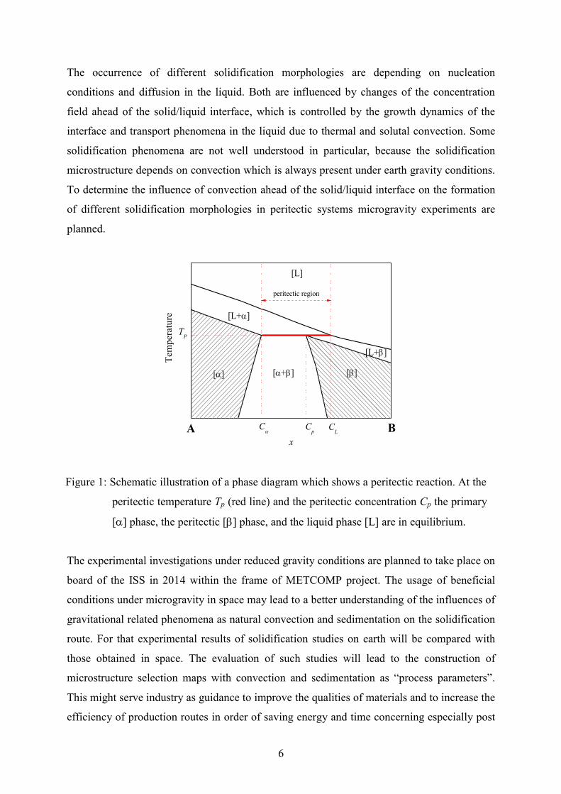
The occurrence of different solidification morphologies are depending on nucleation
conditions and diffusion in the liquid. Both are influenced by changes of the concentration
field ahead of the solid/liquid interface, which is controlled by the growth dynamics of the
interface and transport phenomena in the liquid due to thermal and solutal convection. Some
solidification phenomena are not well understood in particular, because the solidification
microstructure depends on convection which is always present under earth gravity conditions.
To determine the influence of convection ahead of the solid/liquid interface on the formation
of different solidification morphologies in peritectic systems microgravity experiments are
planned.
BCL
C
TP
Cp
[][+][]
[L+]
[L]
[L+]
Tem
pera
ture
x
peritectic region
A
Figure 1: Schematic illustration of a phase diagram which shows a peritectic reaction. At the
peritectic temperature Tp (red line) and the peritectic concentration Cp the primary
[ phase, the peritectic [ phase, and the liquid phase [L] are in equilibrium.
The experimental investigations under reduced gravity conditions are planned to take place on
board of the ISS in 2014 within the frame of METCOMP project. The usage of beneficial
conditions under microgravity in space may lead to a better understanding of the influences of
gravitational related phenomena as natural convection and sedimentation on the solidification
route. For that experimental results of solidification studies on earth will be compared with
those obtained in space. The evaluation of such studies will lead to the construction of
microstructure selection maps with convection and sedimentation as “process parameters”.
This might serve industry as guidance to improve the qualities of materials and to increase the
efficiency of production routes in order of saving energy and time concerning especially post

7
solidification treatment. In microgravity, thermo and solutal convection can be assumed to
have a negligible effect on microstructure formation during peritectic solidification. The
Microgravity Science Glove box (MSG) [1] in the Columbus module (see Figure 2a) on the
International Space Station (ISS) represents a new perspective for the observation of peritectic
solidification. The DIRSOL [1] instrument, a micro Bridgman-furnace, is developed to
perform DIRectional SOLidification experiments on transparent materials in the MSG on
board of the ISS. The DIRSOL facility consists of three major flight parts: The experiment
units with the micro Bridgman-furnace assemble and observation system, the facility control
unit and the DIRSOL cartridges. The mounting configuration inside MSG is shown in Figure
2b. The main diagnostics element of DIRSOL is the optical observation system with high
resolution. The camera can observe the changes in the sample between the hot and cold zones
of the Bridgman assembly at fixed positions and angles.
(a) (b)
Figure 2: (a) MSG isometric view. (b) The DIRSOL facility in grey inside MSG work volume
attached to DIRSOL experiment unit.
In this study, the background of peritectic solidification is reviewed, the suitability of the
selected transparent organic alloy, selected material properties and the reproducibility of
experiments are evaluated. Expected and unexpected solidification morphologies at
solidification rates below the critical velocity are classified.
DIRSOL facility
8
2 State of the Art
Peritectic solidification shows a variety of complex microstructures that is influenced by the
competition between the nucleation and growth of different phases [2]. Investigations on
directional solidification including in-situ observations with X-Ray techniques [3] of
peritectic alloys have been performed on metals like Zn–Ag [4], Sn–Cd [5, 6, 7, 8], Cu-Sn [9],
Pb–Bi [10, 11, 12, 13, 14], Zn–Cu [15, 16, 17], Sn–Sb [18, 19], Ti–Al [20, 21], Fe–Ni [22, 23,
24, 25, 26, 27, 28, 29, 30, 31], Ni–Al [32], YBCO [33] and Nd–Fe–B [34]. Wide spectrums of
complex microstructures were found in directionally solidified alloys and discussed [17, 21,
22, 23, 24, 26, 27, 32, 35, 36, 37, 38] but an in-situ observations of peritectic reactions with
organic compounds was not possible up to now.
2.1 Peritectic Solidification
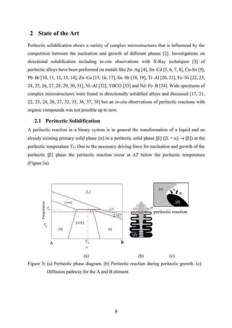
A peritectic reaction in a binary system is in general the transformation of a liquid and an
already existing primary solid phase [to a peritectic solid phase [ ([L + [) at the
peritectic temperature TP. Due to the necessary driving force for nucleation and growth of the
peritectic [] phase the peritectic reaction occur at T below the peritectic temperature
(Figure 3a).
(a) (b) (c)
Figure 3: (a) Peritectic phase diagram. (b) Peritectic reaction during peritectic growth. (c)
Diffusion pathway for the A and B element.
peritectic reaction

9
The peritectic phase diagram is described in detail in Figure 4. The corresponding
concentrations x in mol fraction are C for the [ phase, Cp or C for the peritectic [ phase,
and CL for the liquid phase.
solidification of the
peritectic phase
BCL
C
TP
Cp
[+]
[L+]
[L][L+]
hypo-peritectic
region
hyper-peritectic
regionT
em
pera
ture
x
peritectic region
solidification of the
primary phase
A
Figure 4: Detail of a peritectic phase diagram. At the peritectic temperature Tp and the
peritectic concentration Cp the [], [] and liquid phase are in equilibrium. The
peritectic composition range C to CL can be divided in the hypo-peritectic range
from C to Cp and the hyper-peritectic range from Cp to CL. At concentrations
C0 C, only the [] phase solidifies and for C0 > CL the [] phase grows.
The region C x CL is divided in the hypo-peritectic region C x CP and the hyper-
peritectic region Cp x CL. Whereby, an alloy with a hypo-peritectic concentration C0 with
C C0 CL starts to solidify with the primary [ phase and transforms partly to the
peritectic [ phase when passing Tp [2]. For initial concentrations C0 < C only the [ phase
solidifies and for C0 > CLthe [ phase solidifies. Possible variants for peritectic phase
diagrams are given in Figure 5.
10
[]
[]
B
[+]
[L+]
[L]
[L+]
Tem
pera
ture
xA
[]
[]
B
[+]
[L+]
[L]
[L+]
Tem
pera
ture
xA
[][]
B
[+] [L+]
[L]
[L+]
Tem
pera
ture
xA
(a) (b) (c)
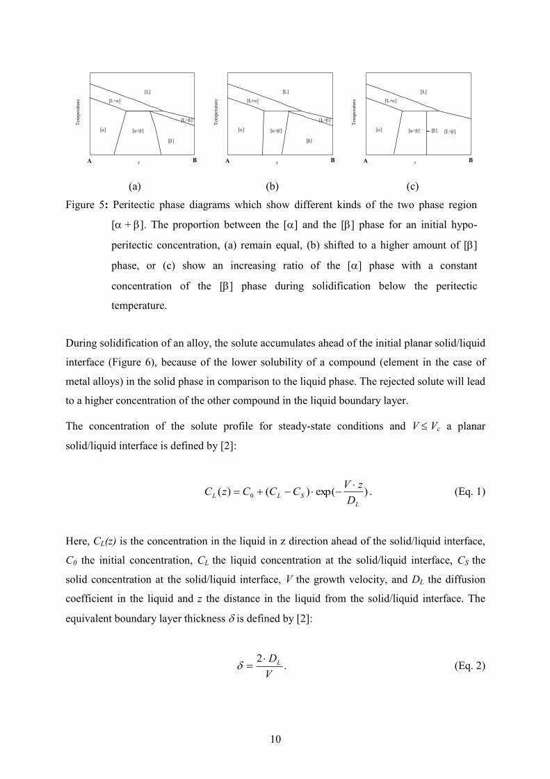
Figure 5: Peritectic phase diagrams which show different kinds of the two phase region
[ + ]. The proportion between the [] and the [] phase for an initial hypo-
peritectic concentration, (a) remain equal, (b) shifted to a higher amount of []
phase, or (c) show an increasing ratio of the [] phase with a constant
concentration of the [] phase during solidification below the peritectic
temperature.
During solidification of an alloy, the solute accumulates ahead of the initial planar solid/liquid
interface (Figure 6), because of the lower solubility of a compound (element in the case of
metal alloys) in the solid phase in comparison to the liquid phase. The rejected solute will lead
to a higher concentration of the other compound in the liquid boundary layer.
The concentration of the solute profile for steady-state conditions and V Vc a planar
solid/liquid interface is defined by [2]:
)exp()()( 0
L
SLLD
zVCCCzC
. (Eq. 1)
Here, CL(z) is the concentration in the liquid in z direction ahead of the solid/liquid interface,
C0 the initial concentration, CL the liquid concentration at the solid/liquid interface, CS the
solid concentration at the solid/liquid interface, V the growth velocity, and DL the diffusion
coefficient in the liquid and z the distance in the liquid from the solid/liquid interface. The
equivalent boundary layer thickness is defined by [2]:
.2
V
DL (Eq. 2)
11
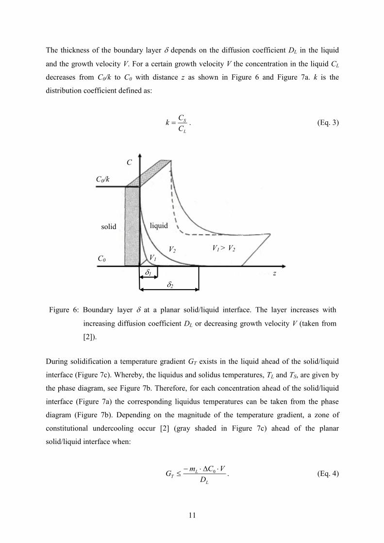
The thickness of the boundary layer depends on the diffusion coefficient DL in the liquid
and the growth velocity V. For a certain growth velocity V the concentration in the liquid CL
decreases from C0/k to C0 with distance z as shown in Figure 6 and Figure 7a. k is the
distribution coefficient defined as:
L
S
C
Ck . (Eq. 3)
Figure 6: Boundary layer at a planar solid/liquid interface. The layer increases with
increasing diffusion coefficient DL or decreasing growth velocity V (taken from
[2]).
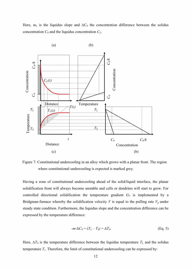
During solidification a temperature gradient GT exists in the liquid ahead of the solid/liquid
interface (Figure 7c). Whereby, the liquidus and solidus temperatures, TL and TS, are given by
the phase diagram, see Figure 7b. Therefore, for each concentration ahead of the solid/liquid
interface (Figure 7a) the corresponding liquidus temperatures can be taken from the phase
diagram (Figure 7b). Depending on the magnitude of the temperature gradient, a zone of
constitutional undercooling occur [2] (gray shaded in Figure 7c) ahead of the planar
solid/liquid interface when:
L
LT
D
VCmG
0 . (Eq. 4)
C0/k
C0
liquid
z
V2 V1
V1 > V2
solid
C
1
2
12
Here, mL is the liquidus slope and C0 the concentration difference between the solidus
concentration C0 and the liquidus concentration CL.
(a) (b)
(c) (b)
Figure 7: Constitutional undercooling in an alloy which grows with a planar front. The region
where constitutional undercooling is expected is marked grey.
Having a zone of constitutional undercooling ahead of the solid/liquid interface, the planar
solidification front will always become unstable and cells or dendrites will start to grow. For
controlled directional solidification the temperature gradient GT is implemented by a
Bridgman-furnace whereby the solidification velocity V is equal to the pulling rate Vp under
steady state condition. Furthermore, the liquidus slope and the concentration difference can be
expressed by the temperature difference:
-mΔC0 = (TL – TS) = T0. (Eq. 5)
Here, T0 is the temperature difference between the liquidus temperature TL and the solidus
temperature Ts. Therefore, the limit of constitutional undercooling can be expressed by:
Concentration
Conce
ntr
atio
n
Conce
ntr
atio
n
Tem
per
ature
Distance
C0/k
C0/k
C0/k
C
0
C0
C0
CL(z)
TL TL
TS TS
TL(z) T(z)
Temperature Distance
z

13
Lc
T
D
T
V
G 0 or
0T
GDV TL
c
. (Eq. 6)
Here, Vc is the critical solidification velocity. At limit of constitutional undercooling, for
V Vc, a stable planar front grows at the corresponding solidus temperature TS of the alloy
[2]. Otherwise, if V Vc, the planar interface becomes unstable and transforms to cells and/or
dendrites to reduce the zone of constitutional undercooling. Whereby, cells and dendrite tip
are growing undercooled in respect to the liquidus temperature TL.
In the peritectic region the values of the two temperature differences, T and T, are
dissimilar (see Figure 8), therefore, for a definite solidification velocity V it is possible that
one phase grows above the limit of constitutional undercooling where the other one grows
below the limit of constitutional undercooling (V
c V V
c for T T).
B
T
C0
[][+]
[][L+]
[L][L+]
Tem
per
atu
re
x
T
A
Figure 8: Temperature difference T and T between the liquidus and solidus line of the
primary [] phase and the peritectic [] phase within the peritectic region. For a
given concentration C0 the temperature difference T depends on the phase with
T .
In this case that the [] phase grows above the limit of constitutional undercooling only the
[] phase grows planar and the [] phase shows cellular or dendritic solidification

14
morphology. The solidification morphology changes to a planar front as soon as the
solidification velocity (V < V
c and V
c) is below the critical velocities of both phases.
The development of the pill-up during the initial transient requires a certain distance of
solidification until the solid/liquid interface can grow under steady-state condition. As a rule
of thumb the necessary transition distance for a planar front to reach steady-state growth
conditions [2] is:
kV
Dz
p
Ltr
6. (Eq. 7)
Here, ztr is the transition length. To determine the time necessary for the solidification front to
reach steady-state the equation above can be transferred to:
kV
Dt
p
Ltr
2
6. (Eq. 8)
Here, ttr is the transition time. Thereafter, the solidification morphology grows under steady-
state condition and forms a diffusion boundary layer with a characteristic length as shown in
Figure 6. In case of cellular or dendritic growth at Vp V,
c, steady-state is reached much
faster than in case of a planar solidification front.
2.1.1 Solidification Rate above the Critical Solidification Velocity Vc, Cells and
Dendrites
A peritectic reaction requires the solidification of liquid and the transformation from the
primary phase [] to the peritectic phase []. The change from the [ phase to the [ phase
is a solid to solid transformation while the transformation from melt to the peritectic [ phase
occurs by solidification. Generally, the solidification and transformation is controlled by
thermal and solute diffusion. Since the thermal diffusion is faster than the solute diffusion, the
solute diffusion is the limiting factor. Besides, the solute diffusion in the liquid is
approximately 1000 times higher than in the solid.
For fast growth conditions (V V
c) the peritectic phase can solidify directly from the melt
or nucleate at the solid/liquid interface, see Figure 9a and b. Another possibility is the

15
solid/solid transformation of the primary [] phase to the peritectic [] phase at temperatures
below the peritectic temperature, see Figure 9c. In Figure 9a the primary [] phase forms cells
or dendrites whereas the peritectic [] phase forms a cellular or dendritic morphology in the
interdendritic or intercellular region. Both phases either grow at the same isotherm or the
peritectic phase is lagging behind the primary phase [39]. As the solidification velocity V
decreases the peritectic solid in between the primary dendrites undergoes a transition from
dendritic to cellular growth and finally to a planar front. For V V
c and V ≤ V
c, the primary
[] phase solidifies still dendritic or cellular while the peritectic [] phase may grow planar.
(a) (b) (c)
Figure 9: Solidification of the peritectic phase for fast growth conditions. (a) The peritectic
phase [] grows directly from the melt. (b) The peritectic phase (gray colored)
solidifies on the solid/liquid interface of the primary phase (white colored). (c) A
solid phase transformation takes place at lower temperature.
Although a microstructure map (depending on temperature gradient GT, pulling velocity Vp,
and initial concentration C0) based on the change in microstructure encountered with single-
phase solidification was proposed by Hunzinger et al. [40], the situation is more complex
since the formation of the [ phase in the intercellular or interdendritic region is controlled
by the diffusion field influenced by the solidifying primary phase.
2.1.2 Solidification Rate below the Critical Solidification Velocity Vc, Layered
Structures
The process conditions for possible band formations are a planar interface for one of the
phases and the absence of convection in the liquid as described in Trivedi [41]. Here, two
metastable two-phase microstructures occur (Figure 10).
[]
[]
[]
[]
16
(a) (b)
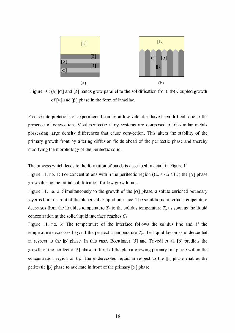
Figure 10: (a) [] and [] bands grow parallel to the solidification front. (b) Coupled growth
of [] and [] phase in the form of lamellae.
Precise interpretations of experimental studies at low velocities have been difficult due to the
presence of convection. Most peritectic alloy systems are composed of dissimilar metals
possessing large density differences that cause convection. This alters the stability of the
primary growth front by altering diffusion fields ahead of the peritectic phase and thereby
modifying the morphology of the peritectic solid.
The process which leads to the formation of bands is described in detail in Figure 11.
Figure 11, no. 1: For concentrations within the peritectic region (C < C0 < CL) the [ phase
grows during the initial solidification for low growth rates.
Figure 11, no. 2: Simultaneously to the growth of the [] phase, a solute enriched boundary
layer is built in front of the planer solid/liquid interface. The solid/liquid interface temperature
decreases from the liquidus temperature TL to the solidus temperature TS as soon as the liquid
concentration at the solid/liquid interface reaches CL.
Figure 11, no. 3: The temperature of the interface follows the solidus line and, if the
temperature decreases beyond the peritectic temperature Tp, the liquid becomes undercooled
in respect to the [ phase. In this case, Boettinger [5] and Trivedi et al. [6] predicts the
growth of the peritectic [ phase in front of the planar growing primary [ phase within the
concentration region of Cb. The undercooled liquid in respect to the [ phase enables the
peritectic [] phase to nucleate in front of the primary [] phase.
[L] [L]
[]
[]
[] [] []
[] []

17
Figure 11: Illustration of the banding process, published in [9], predicted by Trivedi [41] for
concentrations C0 within the concentration region of Cb.
Figure 11, no. 4: Now, with the growth of the peritectic phase the solid composition follows
the solidus line of the [ phase to a higher temperature. Once the temperature of the liquid in
front of the peritectic phase is above the peritectic temperature the [ phase can nucleate
before a steady-state condition for [] growth is obtained. This process leads to the formation
of bands with alternating phases which grow in the form of an oscillating planar front at
temperatures between T
S and T
S (Figure 11, no. 3 and 4).
Trivedi [41] published an equation which can be used to calculate the thickness of bands. The
width of each individual lamella [] and [p] of the [] and [] layers is given by:
.
)m(mC
ΔT(1
C
C1
)m(mC
ΔT(1
C
C1
Λ
][
l
][
l[L]
][
N
0
][
][
l
][
l[L]
][
N
0
][
][
(Eq. 9)
.
)m(mC
ΔT(1
C
C1
)m(mC
ΔT(1
C
C1
Λ
][
l
][
l[L]
][
N
0
[p]
][
l
][
l[L]
][
N
0
[p]
][
(Eq. 10)
C0 C[ C[P] C[L]
TL
TP 2
3
4 T
S
T
S
[L]
[]
[] Cb
1

18
.lnln ][
][
L][
][
L ΛkV
DΛ
kV
Dλ
(Eq. 11)
Here, TNi (i = [] or []) is the undercooling. The assumption of this model is that the
growth of the new nucleated phase in lateral direction VL is rapidly enough to form a new
band before the existing phase overgrow the new nucleated phase, see Figure 12. Note, that in
contrast to Figure 3c on page 8 which shows a peritectic reaction, here, both phases [] and
[] are growing independent.
Figure 12: Competing growth between the primary [ phase and the lateral growth of the
peritectic [ phase in solidification direction. Banded solidification occurs only
if the lateral velocity VL of the new phase [] is faster than the solidification
speed of the existing phase []. Otherwise island bands or coupled growth is
possible.
The growth competition between the nucleated phase and the preexisting phase leads to new
solidification dynamics like coupled growth in a eutectic system (Figure 10b). Dobler [27]
observed such coupled growth in Fe-Ni peritectic alloys.
Prima facie, the coupled growth of a lamellar eutectic system is equal to the solidification
morphology of a coupled growth peritectic system. In both cases, the [ phase grows side by
side with the [ phase. However, in details the coupled growth in a eutectic system differs
from the lamella growth in peritectic systems, see Figure 13. During solidification in eutectic
system the rejected solute in front of the solidifying [ phase is needed by the solidifying [
phase (Figure 13a). In contrast, solidification in the peritectic system requires similar alloy
elements in the solid [ and [ phase. Therefore, the rejected solute in front of the primary
V V
V GT
VL

19
[ phase is not needed to form the peritectic [ phase (Figure 13b). This difference leads to
a much larger boundary layer in front of the solidification front of a peritectic coupled
growth, c 2DL/V, compared to the eutectic solidification with . Furthermore, all
solidification morphologies are highly influenced by the presence of convection and
nucleation ahead of the growing interface [6, 27, 39, 42, 43].
(a) (b)
Figure 13: Formation of the solute layer in front of the solid/liquid interface, published in [9].
(a) Eutectic coupled growth with a solute layer equal to . (b) Peritectic coupled
growth with a much thicker solute layer of 2DL/V.
CL CL
z z
x x
c DL/V

20
2.2 Organic Compounds
Several organic compounds show an orientationally disordered crystal phase (short form
ODIC), usually called plastic crystals [44, 45, 46, 47] or a non-facetted phase (see Figure 14).
Such molecules consist of a pseudo-spherical or globular shape with weakly angle-dependent
interactions usually by van der Waals forces or hydrogen bounds. Plastic crystals can be
considered as an intermediate stage between solid and liquid. They do not have any
orientation order but the positional order still exists, therefore, the molecules are able to
reorient on their lattice site. In a plastic crystal there is a solid lattice with long range
translation symmetry inside which is indicated by sharp Bragg reflections. Molecules in these
phases are more or less free to rotate around their center so that they do act as stacked
spherical objects, therefore, plastic crystals are optically isotropic. The plastic phase is usually
highly symmetrical (etc. cubic) [47, 48].
a) b)
Figure 14: The difference between the solid/liquid interface morphologies for solidification
of a non-facetted phase and a facetted phase can be seen in the growth structure.
a) Solidification of a plastic phase (ODIC) or non-facetted phase happens in the
form of cells similar to metals. b) Growth of a facetted phase or orientationally
ordered crystal. In both cases the pictures show observation results of TRIS ultra-
pure [49].
A convenient criterion for predicting a plastic phase or a facetted phase is the dimensionless
entropy :
R
S f . (Eq. 12)
[L] [L]
non-facetted phase facetted phase

21
Here, Sf is the entropy of fusion and R the gas constant. Values of ≤ 2 imply non-faceted
crystal growth or plastic crystal [2]. The name plastic crystal refers to the same soft plastic
mechanical properties like waxes. This kind of material is very soft and ductile and can be
easily deformed. The molecules reorientate on their lattice position and act in the same way as
metals do [50, 51]. The solidification of the plastic phase follows the same behavior as
observed in metals, namely in form of a planar front, cells, or dendrites depending on the
solidification conditions. Therefore, organic compounds with a plastic phase are quite
attractive to study solidification morphologies with in-situ observation technique. A number
of transparent organic compounds and their alloys have been investigated in [50, 52, 53, 54,
55, 56] to find model substances that allow in-situ and real time observation of metal-like
solidification phenomena such as planar, cellular or dendritic growth. Barrio et al. [57] and
Sturz et al. [52] reported a peritectic reaction for the organic model alloy NPG
(Neopentylglycol)-TRIS (Tris(hydroxymenthyl)aminomethane) and for TRIS
(Tris(hydroxymenthyl)aminomethane) – PE (Pentaery-thritol), see Figure 15.
(a) (b)
Figure 15: (a) The phase diagram of NPG - TRIS (b) The phase diagram of TRIS - PE [57].
All compounds show a plastic phase at high temperature. This fact permits the in-situ
investigation of a non-facetted/non-facetted peritectic phase diagram with the Bridgman
technique. In both diagrams the organic substance TRIS is part of the alloy, a material which
Tem
per
ature
[K
]

22
was never used before for in-situ investigations. Since the temperature range of the peritectic
reaction TRIS – NPG is lower than in the phase diagram TRIS – PE, the phase diagram
TRIS – NPG was chosen in the present thesis for in-situ investigations with the Bridgman
technique.
The binary phase diagram TRIS - NPG was investigated by DSC measurement and X-Ray
patterns and the results are published by Lopez et al. [57, 58]. Also Chandra et al. [59]
investigated the binary phase diagram TRIS – NPG and calculated the binary phase diagram
with the CALPHAD approach and investigated with DSC measurement. All phase diagrams
show differences in the concentrations for the peritectic line and the exact position of the
liquidus and solidus temperatures. Especially, the liquidus line of the pure substance NPG in
the published phase diagram [59] is higher.
Sturz et al. [52] published the thermodynamic data for several organic compounds including
TRIS and NPG. Available information about the physical and chemical properties of TRIS
and NPG are given in Table 7 on page 41.
2.2.1 Organic Compound NPG
Neopentylglycol (formally known as 2,2-dimethyl-1,3propanediol) (CH3)2C(CH2OH)2 has
already been used for this kind of research for a long time and its chemical as well as physical
properties are well known [49]. At 314.6 ± 1.0 K this organic substance transforms from an
ordered low temperature facetted solid phase (phase II) to an orientationally disordered solid
phase (phase I) which is stable up to the melting point at 401.3 ± 1 K. The crystal structure of
the low temperature phase II is monoclinic [M], Z = 4, space group P21/n. Phase I, the plastic
phase (see Figure 14a, page 20), has a face centered cubic structure and is called [CF] with
Z = 4, [57, 58]. The organic substance as delivered from commercial companies has a purity
of 99 % [49]. It is mentioned that thermal decomposition occurs in contact with a strong base
at temperatures higher than 393 K and its decomposition products are methanol, isobutanol,
isobutyl aldehyde, formaldehyde etc. [60]. NPG is very hydroscopic and thus, it usually
contains residual water [61]. This fact requires in any case a pretreatment before it can be
used for further investigations.
2.2.2 Organic Compound TRIS
Tris(hydroxymethyl)aminomethane H2NC(CH2OH)3 is a widely used buffering agent in the
pH range 7 to 9. It is important for studies of physiological media and seawater and

23
commonly known as TRIS or THAM, but formally named 2-amino-2-hytroxymethyl-1,3-
propanediol. With an acid dissociation constant, pKa of 8.3, TRIS is a strong base and has a
good buffer capacity between 7.2 – 9.0 pH. The pKa decreases with approximately
0.03 units/K with increasing temperature [62], therefore, at 393 K TRIS is just a medium
strong base. TRIS is highly hydroscopic, soluble in water and insoluble in alcohol and ether.
The low temperature phase shows an orthorhombic lattice [O] with space group Pn21a and
Z = 4 [57, 58]. It is a facetted phase and appears under polarized light multi-colored (see
Figure 14b, page 20) [61]. The solid/solid transition occurs at 406.8 ± 1.0 K. The high
temperature phase (plastic phase) is body centered cubic [Cl], space group Im3m with Z = 2
and not optical active [57, 58]. Phase II, the low temperature phase, shows strong hydrogen
bonds in the layer and week hydrogen bonds between the layers. The plastic phase [Cl] differs
from other pseudo spherical compounds due to its strong extensive hydrogen bonds.
Hydrogen bonding plays a dominant role in the plastic phase of TRIS and hence the rotational
activation energy is 10 times higher in TRIS than in other plastic crystals [51]. Tamarit et al.
[63] investigated the influence of the dynamic hydrogen bonds on the packing coefficient. It
was shown that the hydrogen bonds control the packing of the molecular crystals and mixed
crystals in the plastic phases. Eilerman et al. [51] investigated the low [O] and high
temperature phase [Cl] of the organic substance. The occurrence of plastic phase stability [Cl]
is quite sensitive to impurities and the sample volume [51]. For three impurities Y-
C(CH2OH)3 different circumstances were observed [51], for Y =
(i) C(CH2OH)3 – CH2OH A reversible transformation to the fcc phase [O] was
reported.
(ii) C(CH2OH)3 – CH2CH3 A glassy state was reported.
(iii) C(CH2OH)3 – CH3 A syrup was formed prior to melting.
This is important because impurities are most likely always present. Wasylishen et al. [64]
investigated the plastic and liquid phase of TRIS and detected an influence of the thermal
history of the sample (with carbon-13 nuclear magnetic resonance spectra). Furthermore,
decomposition of the liquid phase of TRIS was observed [64] indicated by a change from
transparent color to light yellow on. The chemical company DOW reported in their material
safety data sheet (MSDS) [65] that a temperature above 422 K can cause decomposition of
TRIS.
24
In contrast to metals, organic compounds consist of molecules, therefore, they can be thermal
instable and decompose. Thermal instability arises through one of the two mechanisms: (i)
molecular decomposition or self-reaction or (ii) reaction with the molecule with the
environment especially with oxygen [66]. However, TRIS is commercial used at room
temperature, therefore, its properties at higher temperatures are not well studied. Here, TRIS
is used the first time for in-situ observations of solidification morphologies at temperature
above the melting point.
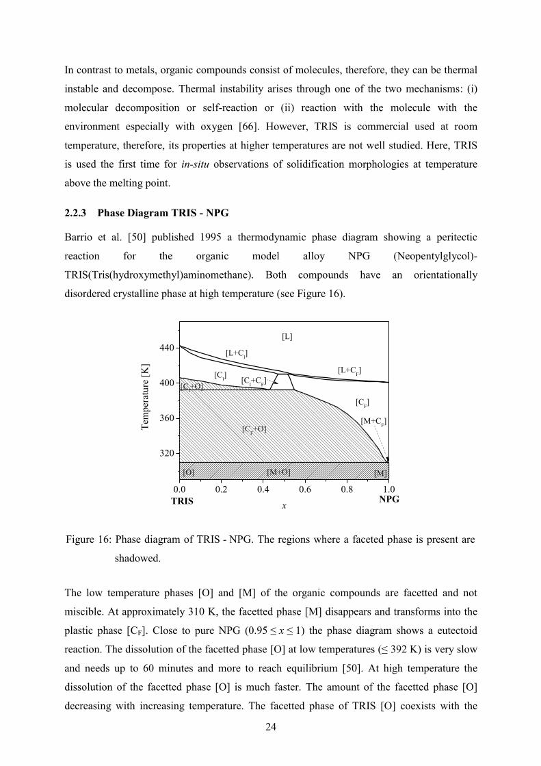
2.2.3 Phase Diagram TRIS - NPG
Barrio et al. [50] published 1995 a thermodynamic phase diagram showing a peritectic
reaction for the organic model alloy NPG (Neopentylglycol)-
TRIS(Tris(hydroxymethyl)aminomethane). Both compounds have an orientationally
disordered crystalline phase at high temperature (see Figure 16).
0.0 0.2 0.4 0.6 0.8 1.0
320
360
400
440
Tem
per
atu
re [
K]
x
[L]
[L+Cl]
[L+CF]
[Cl+C
F]
[Cl]
[Cl+O]
[CF+O]
[CF]
[M+CF]
[M+O][O] [M]
TRIS NPG
Figure 16: Phase diagram of TRIS - NPG. The regions where a faceted phase is present are
shadowed.
The low temperature phases [O] and [M] of the organic compounds are facetted and not
miscible. At approximately 310 K, the facetted phase [M] disappears and transforms into the
plastic phase [CF]. Close to pure NPG (0.95 ≤ x ≤ 1) the phase diagram shows a eutectoid
reaction. The dissolution of the facetted phase [O] at low temperatures (≤ 392 K) is very slow
and needs up to 60 minutes and more to reach equilibrium [50]. At high temperature the
dissolution of the facetted phase [O] is much faster. The amount of the facetted phase [O]
decreasing with increasing temperature. The facetted phase of TRIS [O] coexists with the

25
NPG-rich plastic phase [CF] up to T = 392 K and 0 ≤ x ≤ 0.56. The plastic phase [CF] is stable
up to the melting point between 0.54 ≤ x ≤ 1. At temperatures higher than 392 K, the plastic
phase [CF] transforms to the new plastic phase [Cl] within 0 ≤ x ≤ 0.43 which is stable up to
the melting point. Whereby, the facetted phase [O] disappears above 410 K. Between
0.43 ≤ x ≤ 0.56 and above 392 K both plastic phases [Cl] and [CF] coexist and form a
peritectic plateau at Tp = 410 K and 0.47 ≤ x ≤ 0.54.
The reported phase diagram was constructed from DSC measurements [50] and the evaluation
of the lattice parameters is based on x-ray diffractometry [50]. Figure 17 shows the peritectic
region of the TRIS - NPG phase diagram in detail.
0.4 0.5 0.6
400
405
410
415
420
TP
c[L]
c[CF]
NPGTRIS
[CF][C
l+C
F][C
l]
[L+CF]
[L]
[L+Cl]
c[Cl]
Tem
per
ature
[K
]
x
Figure 17: Peritectic region of the system TRIS - NPG. The squares show the liquidus
(orange), the solidus (red) temperature and the peritectic temperature Tp for the
TRIS-rich side published by [50]. The triangles show the corresponding
situation for the NPG-rich side. The black lines are used to approach the phase
diagram by smooth bended lines and to calculate the distribution coefficient k
and the liquidus sloop m.
The published differences between the solidus temperature and the liquidus temperature are
small and the error bands of both temperatures partly overlap [50]. For calculations the
solidus- and liquidus line have to be approached by smooth bended lines. The calculated
values of the entire phase diagram are given in chapter 4.1 for the distribution coefficient k
(Table 4), the liquidus slope m (Table 5) and the solidus- and liquidus temperature T (Table
2). The red and orange symbols with error bars (Figure 17) are measurements published in

26
[50] and the black lines are the interpolation based on the measurements. Based on the phase
diagram with smooth banded lines, the solute distribution coefficient k and the liquidus slope
mL at the peritectic temperature TP are k[CF] = 0.97 ± 0.01 and m[CF] = -31.0 ± 0.1 K/mol.%,
and also k[Cl] = 0.86 ± 0.01 and mL[Cl] = -47.9 ± 1.4 K/mol.%. The concentrations of the
peritectic plateau C[Cl], C[CF], and C[L] and the peritectic temperature are given in Table 1.
Table 1: Characterization of the peritectic plateau [50].
Peritectic plateau of the phase diagram TRIS - NPG
concentration temperature
C0 x Tp
% mol fraction K
C[L] 54 0.54 410.7 2.0 K
C[CF] 51.5 0.515 410.7 2.0 K
C[Cl] 47 0.47 410.7 2.0 K

27
3 Experimental Methods
3.1 Sample Preparation
The two compounds TRIS and NPG had to be handled in an inert protection atmosphere.
Consequently, the entire preparation was performed within a glove box, consisting of a main
chamber with a removable side wall, two valves for pumping, an argon inlet, and a gate to a
smaller cylindrical flood chamber (Figure 18). The flood chamber itself had two valves for
flooding and pumping. The glove box was filled with Argon 5.6. In order to reduce the
humidity an open container with silica gel was used in order to keep the water humidity below
104 ppm. Several cycles of short evacuation and slow flooding with Argon 5.6 were
performed to reduce the oxygen content from 21 vol.% to a value below 2·103 ppm. Both
values were estimated with a hygrometer. These conditions are kept within the glove box for
all further operations. Experiments outside of the glove box are especially mentioned in the
corresponding chapters.
A side wall B hygrometer C main camber
D gloves E silica gel F flood chamber
Figure 18: Glove box and equipment used for the sample preparation of TRIS - NPG alloys.
D
C A
F
E
B

28
3.1.1 Alloy Preparation
For the same temperature and atmospheric pressure the vapor pressure of NPG and TRIS is
quite different (appendix A.6). Thus, NPG starts to sublimate where TRIS does not.
Therefore, alloy preparation in an open container would lead to a permanent shift in
concentration. As a consequence, it is necessary to prepare the alloys in a small, closed
container (diameter 1 cm, height 5 cm) where it is not possible to lose material by
evaporization. The whole alloy preparation was performed within a glove box, except the
heating and cooling procedure which took place outside the glove box. The accuracy of
concentration of each alloy was checked by DSC measurements.
For the preparation of the different initial alloy compositions, the pure compounds are
weighted (3g) and joined in a small cylindrical glass container closed with a plastic cap (see
Figure 19).
Figure 19: The sketch shows the different steps of the alloy preparation. (a) Total filling of
the empty glass container with NPG and TRIS. (b) Melting of both organic
compounds close to the expected melting temperature. (c) Cooling down and
detach from the glass container. (d) Cut and grinding. (e) Finally, storing for
future use.
Since NPG has a lower melting point than TRIS, NPG was filled into the container first. This
sequence of filling hindered NPG from sublimating before TRIS becomes liquid. The glass
container was heated outside the glove box on a hot plate and as a consequence NPG melts
and TRIS goes partly in solution. Now, the altitude of the liquid alloy was approximately
filling melting
grinding storage
(a) (b)
(c) (e) (d)
cooling down
NPG TRIS
29
1 cm and solid parts of TRIS swam on the liquid surface. Impurities with a boiling
temperature below the melting temperature of NPG were evaporated during melting and
solidified on the cap of the glass container. Then the sample was removed from the heater and
carefully slowly shaken to improve mixing till the last solid part of TRIS was entirely molten.
Subsequently, the solidification started and the sample was slowly cooled down (~ 1 hour).
Finally, the material formed a compact cylindrical alloy within the glass container. The glass
container was crushed in the glove box and a fine thin layer at the top of the cylindrical alloy
was removed. This was done to remove possible impurities from the former liquid surface.
Finally the alloy was ground and filled into a new storage container at atmospheric pressure.
3.1.2 Sample Geometry
Due to the relatively high temperature of the hot zone, 453 K, which is needed to investigate
the solid/liquid interface, all self-produced samples sealed with UV hardening glues and
silica-based glues started leaking after some hours of investigation in the Bridgman-furnace.
Only industrial produced long capillary tubes with glued ends outside of the micro Bridgman
furnace stayed sealed. Samples with an extra-large ratio rectangle tube (100 x 1800 µm2 inner
diameter and 100 µm wall thickness [67]) are used to ensure an optimum of observation area
and a minimum of convection. The sample itself has a length of more than 20 cm and so
10 cm observation length can be used. For simultaneous investigations of samples with
different or equal concentrations square capillary tubes of 0.4 x 0.4 mm2 with a wall thickness
of 0.1 mm were used.
3.1.3 Sample Filling
The sample preparation is performed within a glove box filled with Argon as shown in Figure
18. For the sample filling one end of the glass tube is fixed with a UV hardening glue on a flat
glass plate (60 x 40 x 1 mm). A closed border of glue on the glass plate around the open end
of the tube serves as reservoir for filling as shown in Figure 20. The glass sample is laid on a
hot plate so that the side with the reservoir is heated and the open side freely protrudes the
heated plate. As soon as small amounts of the alloy grains within the reservoir melt the liquid
is dragged into the tube by capillary forces until it reaches the colder end of the tube where it
solidifies. Next, the capillary is slowly dragged off the hot plate and the material solidifies
directionally whereby it shrinks. Consequently, a small part at the end of the sample is
unfilled. The tube is now removed from the glass plate and finally the unfilled ends of the
tube are sealed by gluing. During the investigation in the Bridgman-furnace, both ends of the
capillary tubes extended the hot zone of the furnace and are thus kept close to room

30
temperature. Hence, the solid alloy seals further both ends of the capillary tube and
additionally protects the liquid alloy from any contact with ambient air. After filling, one end
of the tube is glued again on a 2 x 2 cm2 glass plate which serves as handhold. Finally, the
filled and sealed sample is transferred out of the glove box.
Figure 20: Glass plate with glued sample, reservoir and grains of the alloy.
3.2 Differential Scanning Calorimetry (DSC)
For the different scanning Calorimetry (DSC) measurements, 5 mg of each alloy was filled
into small Al pans that were hermetically sealed within the glove box. Next, these DSC
samples were investigated using a Perkin-Elmer Diamond DSC instrument equipped with
Pyris7 Software and calibrated with In and Zn [68]. A similar instrument had been used by
Barrio et al. [50]. The Perkin-Elmer Diamond DSC instrument is a power compensation DSC.
The measuring system consists of two equal micro furnaces. Both furnaces contain a
temperature sensor and a heating resistor (Figure 21).
Figure 21: Power compensation DSC [68]. Set-up of the measuring system. S: sample
measuring system with sample, micro-furnace. R: reference sample system. 1:
heating wire, 2: resistance thermometer. Both systems are in a surrounding block
at constant temperature.
grains of alloy
reservoir
empty sample
glass plate
wall of harding glue
S R
1
2
1
2
31
In one furnace, there is an Al pan with the sample while in the second one there is an empty
Al pan as a reference. During heating-up the same heating power is applied to both micro
furnaces. If a reaction occurs in one of the pans a slide temperature change occurs only in the
sample furnace. Now, the DSC regulation starts to compensate this difference by heating or
cooling. This effect is visible as a peak in the heat flux plot (DSC curve, see Figure 29 on
page 43). The used scanning rate was the same as reported in Ref. [50], i.e. 2 K/min. In the
follow interpretation of the DSC curves will be performed according to the procedure
described in Ref. [68, 69].
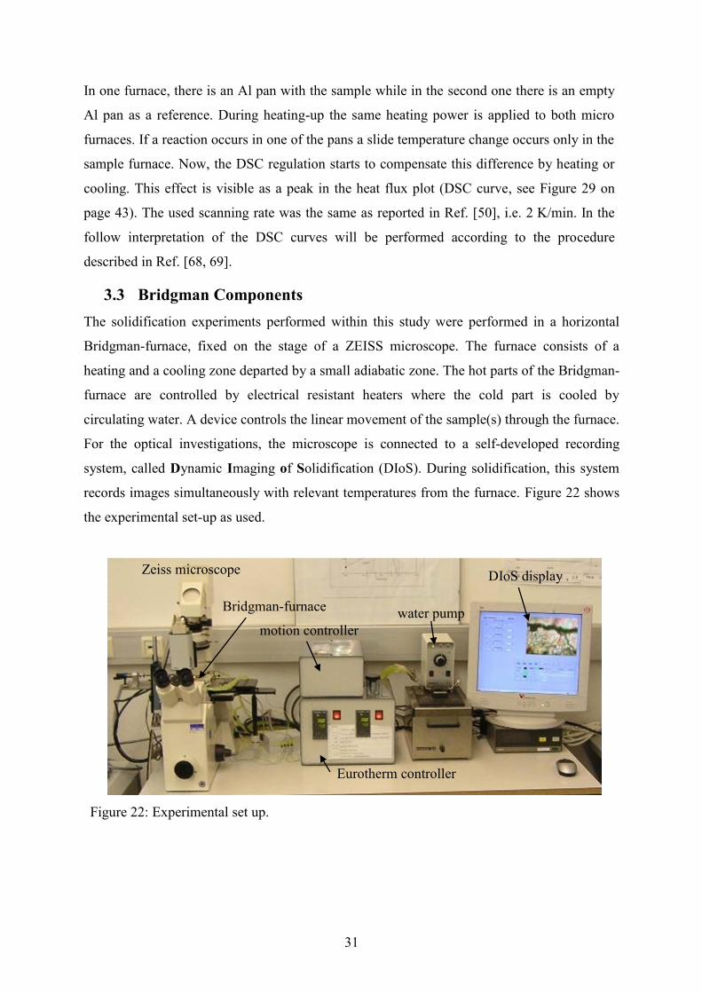
3.3 Bridgman Components
The solidification experiments performed within this study were performed in a horizontal
Bridgman-furnace, fixed on the stage of a ZEISS microscope. The furnace consists of a
heating and a cooling zone departed by a small adiabatic zone. The hot parts of the Bridgman-
furnace are controlled by electrical resistant heaters where the cold part is cooled by
circulating water. A device controls the linear movement of the sample(s) through the furnace.
For the optical investigations, the microscope is connected to a self-developed recording
system, called Dynamic Imaging of Solidification (DIoS). During solidification, this system
records images simultaneously with relevant temperatures from the furnace. Figure 22 shows
the experimental set-up as used.
Figure 22: Experimental set up.
Zeiss microscope DIoS display
Eurotherm controller
motion controller
water pump Bridgman-furnace

32
3.3.1 Micro Bridgman-furnace set up
The horizontal micro Bridgman-furnace is constructed to study directional solidification of
transparent alloys in rectangle or square sample tubes with an observation length of
3.6 0.1mm.
The movement of the capillary tubes through the furnace is PC-controlled using a
FAULHABER DC stepper motor [70] connected to d drive spindle which allows withdrawal
velocities between 0.01 and 115 µm/s. The spindle moves a sledge on which the sample is
fixed. For an experiment a total sample length of 40 mm can be pulled through the adiabatic
gap. Movements in pulling directions are given in the text as a positive value and movements
in the opposite direction as a negative one.
The main parts of the furnace consist of two ceramic plates, each covering a fixed cold and
hot brass block, as shown in Figure 23.
Figure 23: Sketch of the directional solidification apparatus (Bridgman-furnace) used for the
optical investigation of the organic peritectic alloys.
The ceramic plates act in two ways, firstly as thermal isolation, and secondly as a frame to
hold the hot and cold brass blocks. One hot and one cold brass block with a distance of
3.6 mm are permanently mounted within ceramic plates. The bottom plate is permanently
upper ceramic plate
hot zone cold zone
stage
sample
observation field of 3.6 mm bottom ceramic plate ZEISS microscope
hot brass block cold brass block
glass plate
4 mm
illumination
upper ceramic plate

33
connected with the stage of the microscope. The ceramic plate is fixed to the stage only at
four points to reduce the heat conductivity to the microscope. The top plate is placed plane on
top of the bottom plate with a simple plug system. This design allowed a quick change of
samples in the preheated furnace. The hot blocks can be heated up to a maximum temperature
of 523 K using an electric resistant heater. The cold blocks are cooled by a water circuit.
Therefore, the temperature range is limited by the freezing and boiling temperature of water.
The temperatures of the hot zone were measured with Pt-100 temperature sensors placed
inside each brass block and regulated independently by a EUROTHERM 2408 controller [71]
with an accuracy of ± 0.1 °C. The temperature of the cold zone was measured with a Pt-100
temperature sensor placed between the brass blocks and regulated by a water cooling system
with an accuracy of ± 0.5 °C measured within the water tank of the pump. A slot of
0.4 x 2 mm2 is milled in the hot and cold brass block of the bottom ceramic plate to host the
samples. The width of the slot allows the investigation of a rectangular glass capillary
0.3 x 2 mm2 (0.1 x1.8 mm
2 with 100 µm wall thickness) or simultaneous investigation of up
to five square capillaries of 0.4 x 0.4 mm2 (0.2 x0.2 mm
2 with 100 µm wall thickness).
Additionally, two parallel slots are at the bottom part of the brass blocks. During the
experiments, two short filled glass samples (0.4 x 0.4 mm2) with pure NPG and pure TRIS
laid unmoved in the additional slots because the phase transition boundaries, solid/liquid for
NPG and solid/solid for TRIS, where used to check the stability of the temperature gradient
(see chapter A.8). Figure 24 gives detailed information about the construction.
Figure 24: Picture of the bottom ceramic plate, the hot and cold brass blocks, a filled
rectangular glass sample, and the pulling system.
ceramic plate
hot brass
block
Pt 100
sample
adiabatic zone
extra slots 40 mm
start- and end position of the sledge
spindle
34
The size of the glass sample hinders the usage of micro temperature sensors to estimate the
temperature gradient within the adiabatic zone. With additional spacers on the hot and cold
brass block, the furnace is also suitable for a 0.8 x 3.5 mm2 rectangular tube. The larger
sample shape enables the application of temperature sensor.
3.3.2 Optical Observation System “DIoS”
The ZEISS microscope was equipped with a CCD camera and two crossable polarization
filters. The filters are used to distinguish between the optical active and inactive solid phases
as described in Figure 14. Without the usage of the filters all phases are visible but with two
90° crossed filters only the optically active phases can be seen. A self-developed software
records and stores images and the corresponding temperature data with a frame rate of up to
10 images per second. In the gap (3.6 mm) between the hot and the cold brass blocks the
samples were illuminated from the bottom and observed from the top with the used ZEISS
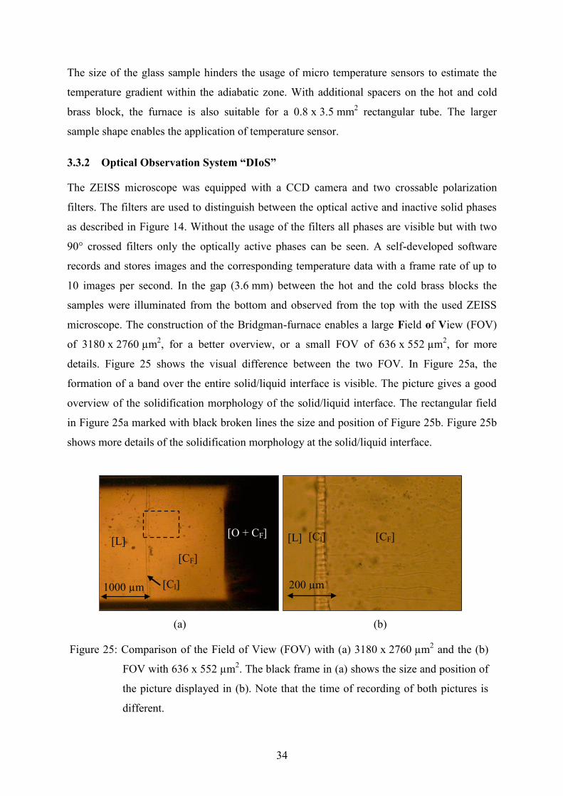
microscope. The construction of the Bridgman-furnace enables a large Field of View (FOV)
of 3180 x 2760 µm2, for a better overview, or a small FOV of 636 x 552 µm
2, for more
details. Figure 25 shows the visual difference between the two FOV. In Figure 25a, the
formation of a band over the entire solid/liquid interface is visible. The picture gives a good
overview of the solidification morphology of the solid/liquid interface. The rectangular field
in Figure 25a marked with black broken lines the size and position of Figure 25b. Figure 25b
shows more details of the solidification morphology at the solid/liquid interface.
(a) (b)
Figure 25: Comparison of the Field of View (FOV) with (a) 3180 x 2760 µm2 and the (b)
FOV with 636 x 552 µm2. The black frame in (a) shows the size and position of
the picture displayed in (b). Note that the time of recording of both pictures is
different.
[L] [L]
[CF]
[CF] [Cl]
[Cl]
[O + CF]
1000 µm 200 µm

35
In this work, pictures with the lager field of view are aligned to thick red (hot) and blue (cold)
lines for the indication of the position of the corresponding copper blocks of the Bridgman-
furnace. The small construction of the adiabatic gap limits the optical magnification.
A measurement facility was developed to enable the recording of digital images and the
corresponding temperatures. The DIoS system was assembled by the Institute for Automation
at the University of Leoben [72]. It is equipped with 4 PT-100 temperature resistances, a ½”
Pulnix TMC-6700 digital camera. The camera itself has a resolution of 648 x 484 pixels and
the software was programmed in MATLAB [72]. Figure 26 shows the display of the
recording system. On the right side, the area of observation (FOV) and on the left side, the
reading of up to 4 Pt-100 temperature sensors can be displayed and triggers can be set. It is
possible to trigger the recording of images and temperatures via a start or end temperature.
Figure 26: Display of the DIoS system and the field of view (FOV) of the microscope.
Below the image display the timescale of the recordings can be chosen from images taken
every tenth of a second up to hours. The software stores up to 3000 pictures per run.
Furthermore the software allows the setting of measurement positions in the field of view,
which in combination with the fixed temperature gradient, can be used to estimate the
temperature on a certain position.
recording of the temperature in the hot and cold zone of the cooper block
FOV
storage system

36
4 Stability and Reproducibility of the NPG – TRIS System
NPG was already investigated in several in-situ experiments and has been used for years
without any problems. TRIS is known to be a buffer agent but in literature up to now nothing
has been reported about its application for in-situ observation experiments. The present thesis
is based on studies which was performed in order to define process conditions for in-situ
observations of peritectic solidification morphologies in a micro Bridgman-furnace for the
system TRIS - NPG. The qualities of organic substances differ between several production
charges. Therefore, experiments were done to compare published values. The appendix
includes the effect of different material purification and the colorization of the phases for
better visual observations, the determination of the boiling point, the Raman spectra, the heat
conductivity, the vapor pressure, the viscosity, and the diffusion coefficient in the liquid.
This section contains the collection of all available material safety data sheets (MSDS) of the
pure compounds, details of the phase diagram TRIS – NPG, the stability and reproducibility
of the NPG – TRIS alloys, possible operation conditions and the selected experimental
procedure.
4.1 Phase Diagram of TRIS – NPG
The published phase transition temperatures at selected concentrations from Barrio et al. [50]
include error bars which are not shown in the diagrams in the presented study. For
simplification, the published phase diagram [50] was changed from NPG – TRIS (Figure 15
on page 21) to TRIS – NPG (Figure 16 on page 24). Furthermore the published solidus and
liquidus temperatures intervals were connected by smoother lines. From these lines the
average solidus and liquidus temperatures (Table 2), also the distribution coefficient k and k
(Figure 27, Table 4) and the liquidus and solidus slopes m
l, m
s, m
l and m
s (Figure 28,
Table 5) were calculated. Table 6 shows the estimated values of the diffusion coefficient DL in
the liquid from chapter A.9 and the calculated critical velocity Vc.

37
Table 2: Liquidus temperature, solidus temperature and T estimated by smoothing of
information of the phase diagram published in [50]. Values in bracket show
metastable extensions.
x liquidus
temperature
solidus
temperature T
liquidus
temperature
solidus
temperature T
phase [CF] phase [CF] phase [Cl] phase [Cl]
mol fraction K K K K K K
0.000 442.95 442.95 0.00
0.010 441.85 441.05 0.80
0.025 440.45 438.55 1.90
0.050 438.25 434.65 3.60
0.100 434.15 429.15 5.00
0.200 427.15 423.35 3.80
0.300 422.20 418.15 4.05
0.400 417.25 413.95 3.30
0.450 415.05 411.65 3.40
0.470 414.05 410.70 3.35
0.475 413.85 (410.50) (3.35)
0.500 (411.80) (411.40) (0.40) 412.65 (409.50) (3.35)
0.515 (411.40) (410.70) (0.70) 411.89 (408.80) (3.35)
0.525 (410.90) (410.20) (0.70) 411.46 (408.40) (3.35)
0.540 410.7 409.65 1.05 410.70 (407.70) (3.35)
0.550 410.35 409.2 1.15
0.600 408.85 407.15 1.70
0.650 407.35 405.4 1.95
0.700 406.2 404.05 2.15
0.750 405.25 403.25 2.00
0.800 404.45 402.65 1.80
0.850 403.55 402.25 1.30
0.900 402.75 401.8 0.95
0.950 401.95 401.35 0.60
0.975 401.55 401.25 0.30
0.990 401.15 401.15 0.00
1.000 401.15 401.15 0.00
Table 3: Liquidus temperature, solidus temperature and T estimated by own DSC
measurement.
x liquidus
temperature
solidus
temperature T x
liquidus
temperature
solidus
temperature T
phase [Cl] phase [Cl] phase [CF] phase [CF]
mol
fraction K K K
mol
fraction K K K
0.000 441.6 0.6 410.9 406.2 4.7
0.100 434.9 429.1 5.8 0.7 408.6 404.1 4.5
0.200 428.2 421.6 6.6 0.75 407.3 403.1 4.2
0.300 423.6 418.6 5 0.8 406.3 402.1 4.2
0.400 419 414.1 4.9 0.85 405 401.6 3.4
0.450 416.4 409.1 7.3 0.9 403.7 400.1 3.6
0.470 415.3 409.1 6.2 0.95 403.7 401.1 2.6
0.460 415.6 411.6 4 1 400.9
0.500 412.5 408.6 3.9
0.520 412.8 409.6 3.2

38
0.0 0.2 0.4 0.6 0.8 1.0
0.0
0.2
0.4
0.6
0.8
1.0
1.2
x
dis
trib
uti
on c
oef
fici
ent
k
bcc structure fcc structure
[CF]
[Cl]
Figure 27: Calculated solute distribution coefficient ki of the phase diagram TRIS - NPG
depending on the mol fraction x.
Table 4: Calculated values of the solute distribution coefficient ki of the phase diagram TRIS
- NPG as shown in Figure 27. Values in bracket show metastable extensions.
bcc structure (TRIS rich) fcc structure (NPG rich)
x kL ±
x kL ±
mol fraction mol fraction
0.010 0.40 2.010-02
0.500 (0.89) 1.010-02
0.025 0.43 2.010-02
0.540 0.96 1.010-02
0.050 0.48 2.010-02
0.550 0.95 1.010-02
0.100 0.54 2.010-02
0.600 0.93 1.010-02
0.200 0.66 2.010-02
0.650 0.92 1.010-02
0.300 0.75 1.010-02
0.700 0.89 1.010-02
0.400 0.81 1.010-02
0.750 0.88 1.010-02
0.450 0.84 1.010-02
0.800 0.86 1.010-02
0.470 0.84 1.010-02
0.850 0.86 1.010-02
0.475 0.85 2.010-02
0.890 0.87 1.010-02
0.500 0.86 1.010-02
0.900 0.89 1.010-02
0.515 0.86 2.010-02
0.950 0.93 1.010-02
0.525 0.87 1.010-02
0.975 0.97 1.010-02
0.530 0.86 1.010-02
0.540 0.87 1.010-02
39
0.0 0.2 0.4 0.6 0.8 1.0-200
-150
-100
-50
0
[CF]
[Cl]
peritectic region
li
quid
us/
soli
dus
slope
[K/m
ol]
x
liquidus slope
solidus slope
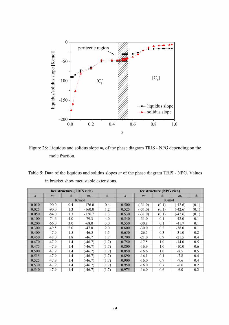
Figure 28: Liquidus and solidus slope mi of the phase diagram TRIS - NPG depending on the
mole fraction.
Table 5: Data of the liquidus and solidus slopes m of the phase diagram TRIS - NPG. Values
in bracket show metastable extensions.
bcc structure (TRIS rich) fcc structure (NPG rich)
x ml ± ms ± x ml ± ms ±
K/mol K/mol
0.010 -90.0 0.4 -176.0 0.4 0.500 (-31.0) (0.1) (-42.6) (0.1)
0.025 -90.0 1.3 -160.0 1.2 0.525 (-31.0) (0.1) (-42.6) (0.1)
0.050 -84.0 1.3 -126.7 1.3 0.530 (-31.0) (0.1) (-42.6) (0.1)
0.100 -74.6 4.0 -79.3 4.0 0.540 -31.0 0.1 -42.0 0.1
0.200 -66.0 3.0 -68.0 3.0 0.550 -30.8 0.1 -41.7 0.1
0.300 -49.5 2.0 -47.0 2.0 0.600 -30.0 0.2 -38.0 0.1
0.400 -47.9 1.5 -46.5 1.5 0.650 -26.5 0.3 -31.0 0.2
0.450 -48.0 1.8 -46.7 1.7 0.700 -21.0 0.9 -21.5 0.4
0.470 -47.9 1.4 (-46.7) (1.7) 0.750 -17.5 1.0 -14.0 0.5
0.475 -47.9 1.4 (-46.7) (1.7) 0.800 -16.9 1.0 -10.0 0.6
0.500 -47.9 1.4 (-46.7) (1.7) 0.850 -16.6 1.0 -8.5 0.5
0.515 -47.9 1.4 (-46.7) (1.7) 0.890 -16.1 0.1 -7.8 0.4
0.525 -47.9 1.4 (-46.7) (1.7) 0.900 -16.0 0.7 -7.6 0.4
0.530 -47.9 1.4 (-46.7) (1.7) 0.950 -16.0 0.7 -6.6 0.2
0.540 -47.9 1.4 (-46.7) (1.7) 0.975 -16.0 0.6 -6.0 0.2

40
Table 6: Corresponding to Eq.6 in chapter 2.1 the estimated values of the critical velocity Vc
of the binary phase diagram TRIS - NPG. Values in bracket show interpolated
values.
x phase [Cl] (TRIS rich) phase [CF] (NPG rich)
mol
fraction DL G/V Vc DL G/V Vc
NPG m2/s sK/m
2 µm/s m
2/s sK/m
2 µm/s
0.050 4.010-11
9.010-11
0.16
0.100 3.410-11
1.510-11
0.10
0.200 3.810-11
1.010-11
0.15
0.300 3.010-11
1.310-11
0.11
0.400 3.210-11
1.010-11
0.14
0.450 2.810-11
1.210-11
0.12
0.470 2.910-11
1.210-11
0.13
0.475 (2.810-11
) 1.210-11
0.12
0.500 2.010-11
1.710-11
0.09 2.010-11
2.010-10
0.73
0.515 (1.710-11
) 1.910-11
0.08 1.710-11
(4.110-10
) 0.35
0.525 1.610-11
2.110-11
0.07 1.610-11
(4.310-10
) 0.33
0.540 (1.310-11
) 2.610-11
0.06 1.310-11
8.010-10
0.18
0.550 1.310-11
(8.710-10
) 0.17
0.600 1.410-11
1.210-11
0.12
0.650 2.010-11
(9.710-10
) 0.15
0.700 2.610-11
8.310-10
0.18
0.750 2.810-11
(7.110-10
) 0.20
0.800 3.010-11
6.010-10
0.24
0.850 3.410-11
(3.810-10
) 0.38
0.900 4.410-11
(2.110-10
) 0.68

41
4.2 Available Physical and Chemical Properties of TRIS and NPG
Table 7 shows published chemical and physical properties of the organic compounds TRIS
and NPG. Some data are only available online [49, 65] whereby other information are based
on direct contact with the producing company.
Table 7: Published chemical and physical properties of TRIS - NPG.
TRIS NPG
Formula [49] H2NC(CH2OH)3 (CH3)2C(CH2OH)2
Formula, summed up [49] C4H11NO3 C5H12O2
CAS-Nr. [49] 77-86-1 126-30-7
Structure [49]
Sigma Aldrich Prod. Nr. [49] T1503 53.825-6
Purity as delivered [49] 99.9+ % 99 %
Density at room temperature [49] 1.353 g/cm3 0.980 g/cm
3
Molar mass [62] 121.14 g/mol 104.15 g/mol
Tm (as delivered) [49] 445 - 446 K 398 - 403 K
Low temperature phase [57] Orthorhombic [O] Monoclinic [M]
Lattice constants [57]
a = 8.853 Å
b = 7.804 Å
c = 8.800 Å
a = 6.019 Å
b = 10.881 Å
c = 10.132 Å
= 100.160 Å
TSST (s.-s. transition) [57] 406.8 1.0 K 314.6 1.0 K
HSST [57] 34.0 1.7 kJ/mol 12.8 0.6 kJ/mol
SSST [63] 83.7 J/mol·K 40.6 J/mol·K
VSST [63] 5.07 cm3/mol 4.86 cm
3/mol
HSST [57] 3.7 0.2 kJ/mol 4.4 0.2 kJ/mol
High temp phase [57] bcc [Cl] fcc [CF]
Lattice constant [57] 6.8888 Å (at 408 K) 8.854 Å (at 353 K)
Tm (purified) [57] 442.7 1.0 K 401.3 1.0 K
Hm [57] 3.7 0.2 kJ/mol 4.4 0.2 kJ/mol
Sm [63] 7.12 J/mol·K 10.8 J/mol·K
Vm [63] 6.63 cm3/mol 4.86 cm
3/mol
Tb (as delivered) [49] 492 - 493 K (at 13 hPa) 481 - 482 K
Sf [73] 1.06105 J/Km
42
4.3 Investigation on the Organic Material
This section includes the effect of material purification and experiments to determine the
reproducibility of the phase diagram, and thermal stability for long time experiments,
4.3.1 Material Purification
NPG and TRIS were delivered with a purity of 99 % and 99.9+ %, respectively. Efforts were
made to increase the level of purity of both organic substances, see appendix A.1. The organic
substance NPG was treated in two ways, by a drying process and by sublimation and
deposition. The achieved purity was tested by DSC measurements. The change of the melting
temperature was marginal and within the error of the DSC evaluation. Therefore, NPG was
purified only by a long time drying process within the glove box, similar to the work
described in [50].
TRIS is reported to be a hygroscopic material [61] and the plastic phase of the organic
substance TRIS is quite sensitive to impurities [51, 64] and decomposes after several hours. A
drying process at 310 K shows no optically visible effect within 24 hours. At a temperature of
373 K, the solid material becomes soft and liquid after 24 hours, whereby the published
melting temperature is 445 K [50]. This could be an indicator for the reported thermal
instability of TRIS at higher temperature [51, 64, 65]. A purification of TRIS by sublimation
and subsequent solid deposition is not possible because TRIS decompose visible by long
brown/white facetted organic crystals. Since TRIS as delivered has already a purity of
99.9+ %, TRIS ultra-pure [49] and to avoid decomposition, TRIS was used as delivered
without any further purification.
4.3.2 Reproducibility of the Alloy Concentration
In order to check the reproducibility of the alloy concentration, DSC measurements were
performed. Various alloy compositions were prepared in the glove box and stored in glass
containers.
The top of Figure 29 shows the original heat flow plot where the peak represents the change
in the heat flux curve due to a phase transition (e.g. from a solid to the liquid phase), the curve
below shows its first derivative.

43
Tm
Tm
Ti
Ti
TSST
Tc
Te
Tc
Te
TL=(T
m + T
e)/2
Hea
t fl
ow
Temperature
1st derivative
inflection points
TSbase line
tangent
Figure 29: Sketch illustrating how transition temperatures have been extracted from a DSC
heating curve, Ti : Initial peak temperature, Te: extrapolated peak onset
temperature, Tc: extrapolated peak completion temperature, TSST: solid state
transformation temperature, TS: solid temperature and TL: liquidus temperature.
Without a phase transition (i.e. in the regions before and after the peaks) the heating curve
corresponds to the heat absorbed by the corresponding phase. Since the applied heat increases
linearly, the corresponding heat flow curves before and after the transitions are resulting in
two different baselines, whereby, the difference in the baselines is caused by the different heat
capacities of the phases. Ti defines the beginning of the first melting, the maximum and the
minimum of the first derivative give the inflection points of the phase transition peak. The
inflection point of the first derivative defines the maximum of the phase transition peak Tm.
The intersection points between the baselines and the corresponding tangents are the points
where the phase transition starts (Te) and ends (Tc).
Sturz et al. [52] obtained the solid transformation temperature and the melting point for the
organic substance TRIS from the extrapolated peak onset temperature Te. Due to the relatively
small liquidus/solidus separation, the DSC measurements reveal only single peaks for the
transition from liquid to solid. Boettinger et al. [69] showed that for small freezing ranges the
maximum peak temperature lies above the liquidus temperature with an error increasing as the

44
freezing interval decreases. Therefore, it can be concluded that the true liquidus temperature
lies between the lower temperature onset point and the maximum peak temperature. This is
reflected in the error bar for the liquidus temperature (see Figure 31). The solidus temperature
was taken at the first deviation from the base line of the DSC curve performed identically in
[69]. For a solid state transformation (TSST) the first onset point Te was taken. Furthermore, the
transition curves for the solid/solid transition often show shoulders indicating a superposition
of multiple peaks. In these cases the onset of the phase transition was taken from the lowest
temperature peak. Due to the overlap of the peaks, the transition temperature of the next peak
segment was approximated with a tangent from the top of the shoulder peak segment.
Samples taken from the same alloy preparation showed a standard deviation of 0.7 K for the
liquidus temperature and 1.1 K for the solidus.
In Figure 30, DSC tracers for the different regions of the peritectic phase diagram are
presented. The solid/liquid transition generally showed a clearly distinguishable single peak.
Therefore, this transition was the best for a direct comparison with the phase diagram
published by Barrio et al. [50].
370 380 390 400 410 420 430 440 450
liq
uid
peritectic
liq
uid
CF
CI
CF +
CI
CI +
O
100% NPG
40% NPG
30% NPG
20% NPG
10% NPG
48% NPG
50% NPG
51% NPG
60% NPG
70% NPG
75% NPG
80% NPG
85% NPG
90% NPG
95% NPG
Hea
t fl
ow
[ar
bit
rary
un
its]
Temperature [K]
100% TRIS
CF +
O
Figure 30: DSC heating curves obtained with various alloy compositions and a heating rate of
2 K/min for the binary phase diagram TRIS – NPG.

45
Compositions ranging from 0 ≤ x ≤ 0.48 mol fraction NPG showed overlapping peaks for the
solid/solid transition and a clearly detached solid-liquid transition peak. The compositions at
the peritectic plateau showed clearly distinguishable single solid/solid and solid-liquid
transition peaks. The compositions from 0.65 ≤ x ≤ 1 mol fraction NPG showed no clearly
distinguishable solid/solid transition but a clear solid/liquid transition peak.
The comparison of the phase diagram derived from these DSC measurements (Figure 31) with
the phase diagram that was elaborated by X-ray diffraction and DSC measurements and
published by Barrio et al. [50] gives good agreement for the liquidus line and the lowest
temperature solid/solid transition line which was denoted as the [CF+O] to [Cl+O] phase
transition by Barrio et al. [50]. The reported phase diagram could be confirmed by our DSC
measurement.
0.0 0.1 0.2 0.3 0.4 0.5 0.6 0.7 0.8 0.9 1.0
380
390
400
410
420
430
440
450
TRIS NPG
Tem
per
atu
re [
K]
x
[CF+O]
[L+Cl]
[L]
[L+CF]
[CF]
[Cl]
[Cl+O]
[CF+C
l]
Figure 31: Phase diagram derived from DSC measurements (points with error bars) and
comparison with the diagram published in [50] (lines with dotted error bands).
46
4.3.3 Thermal Stability
Up to now, no other organic model alloy with a non-facetted/non-facetted peritectic reaction
was investigated. Trivedi et al. [41] presented experimental evidence for banded structure
formation during directional peritectic solidification in metals. These experiments required
several hours for the formation of alternating bands [6, 39, 42]. Unfortunately, the Dow
Chemical Company [65] propose a decomposition temperature for TRIS at 422 K. Depending
on the liquidus temperature of the phase diagram TRIS - NPG, alloys with a concentration of
x > 0.3mol fraction NPG (including concentrations within the peritectic region), melt below
this temperature. Whereas alloys with a higher TRIS content, x 0.3 mol fraction NPG melt
above the decomposition temperature. To clarify a possible decomposition of TRIS during
solidification experiments, annealing DSC measurements, heating cycles DSC measurement
and annealing investigations in a furnace were performed [66]. In addition, the influence of
heating of TRIS was investigated by Raman spectroscopy.
Annealing DSC measurements
To establish the thermal stability of the molecules of NPG and TRIS separate DSC
measurements have been performed. A thermal stability investigation DSC with a very fast
heating rate of 16.610-2
K/s (10 K/min) was selected. At the selected temperatures (473, 463
and 453 K) the pure materials and the representative alloys (x = 0.3, 0.5, and 0.7 mol fraction
NPG) were exposed to the temperature for several hours. As long as no reaction occurs, the
DSC curve should be a straight line. In the case of a chemical reaction a peak appears.
Figure 32 summarizes the isothermal DSC measurement obtained for pure NPG, pure TRIS,
and an alloy with x = 0.50 mol fraction NPG within the peritectic region. The flat DSC lines
for pure NPG (dotted red lines in Figure 32) indicate that NPG is stable up to 473 K, which
correspond to 10 K below the boiling point of NPG, for more than 4 hours. The DSC curves
for pure TRIS (continuous solid line) show that some changes occur after 60 minutes in TRIS
when it is exposed to a temperature of 473 K (i.e. 20 K below the boiling point). Upon
reducing the exposure temperature to 463 K and 453 K (10 K above its melting point) the
stability time of TRIS gradually increased to 3 and more than 4 hours, respectively.
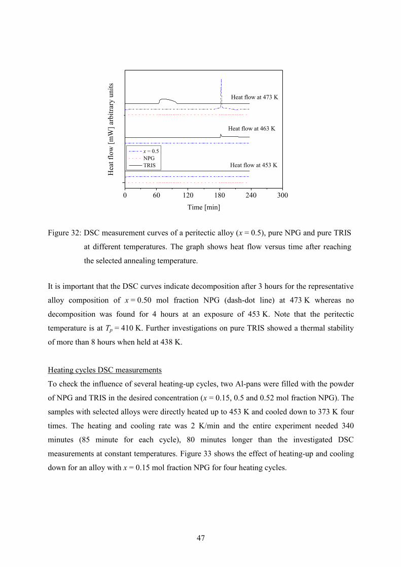
47
0 60 120 180 240 300
Heat flow at 453 K
Heat flow at 463 K
Hea
t fl
ow
[m
W]
arb
itra
ry u
nit
s
Time [min]
x = 0.5
NPG
TRIS
Heat flow at 473 K
Figure 32: DSC measurement curves of a peritectic alloy (x = 0.5), pure NPG and pure TRIS
at different temperatures. The graph shows heat flow versus time after reaching
the selected annealing temperature.
It is important that the DSC curves indicate decomposition after 3 hours for the representative
alloy composition of x = 0.50 mol fraction NPG (dash-dot line) at 473 K whereas no
decomposition was found for 4 hours at an exposure of 453 K. Note that the peritectic
temperature is at Tp = 410 K. Further investigations on pure TRIS showed a thermal stability
of more than 8 hours when held at 438 K.
Heating cycles DSC measurements
To check the influence of several heating-up cycles, two Al-pans were filled with the powder
of NPG and TRIS in the desired concentration (x = 0.15, 0.5 and 0.52 mol fraction NPG). The
samples with selected alloys were directly heated up to 453 K and cooled down to 373 K four
times. The heating and cooling rate was 2 K/min and the entire experiment needed 340
minutes (85 minute for each cycle), 80 minutes longer than the investigated DSC
measurements at constant temperatures. Figure 33 shows the effect of heating-up and cooling
down for an alloy with x = 0.15 mol fraction NPG for four heating cycles.

48
416 420 424 428 432 436 440 444
Hea
t fl
ow
[ar
bit
rary
un
its]
Temperature [K]
1st heating-up 2
nd heating-up
3rd
heating-up 4th heating-up
1T
l = 428.0 ± 1 K
2T
l = 426.2 ± 1 K
3T
l = 422.0 ± 1 K
4T
l = 418.2 ± 1 K
1T
l = 433.0 ± 1.7 K
2T
l = 432.2 ± 3.5 K
2T
l = 431.4 ± 4.3 K
2T
l = 430.0 ± 4.3 K
x = 0.15
Figure 33: DSC curve of a sample with x = 0.15 mol fraction NPG. The sample was heated
up and cooled down four times. The liquidus and solidus temperature decreased
after each cycle.
The estimated liquidus and solidus temperature decreased for each DSC measurement cycle.
In combination the variance increased from 1.7 K to 4.3 K. The variance can be used as an
indication for the amount of impurities within the sample [68]. The same happens with other
tested concentrations. The decreasing solidus and liquidus temperatures illustrate an
increasing amount of impurities. Since the samples were sealed, the additional impurities are
thought to be caused by thermal instability of the organic substances TRIS and/or NPG. As a
consequence samples can be used only for a single experimental run and should not be longer
investigated than 4 hours at a temperature of 453 K otherwise the investigation results are
questionable.
Annealing furnace investigations
For the annealing experiments several glass bottles (5 cm diameter, 5 cm high) were filled
with 25 g TRIS, sealed and kept for 24 hours at 435 K, 425 K, 415 and 405 K. The error bars
for all temperatures are smaller than 1 K. The first three selected temperatures are in the
plastic phase region whereas the last one is below the solid/solid transition. All samples kept
above the solid/solid transition temperature transformed from the faceted phase to the plastic
phase and the samples kept at an annealing temperature at 435 K and 425 K became finally
49
liquid. The sample kept at an annealing temperature of 415 K became waxier (softer) and then
liquid. During the investigations, the color of the material changed from transparent to opaque
and finally to brown. Only the sample at the annealing temperature below the solid/solid
transition temperature stayed solid within 24 hours.
Raman spectroscopy
Raman spectroscopy (see appendix A.4) was used to investigate the decomposition because
each material shows a typical vibration band, like a finger print. Therefore, pure TRIS and an
alloy with a high concentration of TRIS were prepared and investigated. Subsequently, TRIS
and the alloy were heated and hold for selected temperatures for several hours. During this
time the color of TRIS and the alloy changed from opaque to brown. After cooling, the
spectrum of TRIS and the alloy were again determined. Pure unheated TRIS shows a Raman
spectrum without fluorescence but used TRIS, prepared alloy, and the in solidification
experiments used alloy show in their Raman spectra a strong fluorescence. Furthermore, the
Raman spectra show small differences in the Raman intensity between the molten substance
and the substance as delivered. This indicates that TRIS is affected after melting.
Summary
DSC isothermal annealing showed that NPG was stable for more than 4 hours at temperatures
up to 473 K. TRIS, on the contrary, showed decomposition depending on the applied
temperature. At a hot zone temperature of 453 K selected samples were chemically stable for
4 hours. Investigations of heating and cooling cycles show a small declination of the liquidus
and solidus temperature after each cycle. As a consequence samples can be used only for a
single experimental run and should not be longer investigated than 4 hours at a temperature of
453 K or lower.

50
4.4 Corresponding Consequences
4.4.1 Conclusions from the Thermal Stability Investigation
Based on the investigation it can be stated that TRIS restricts the solidification studies in this
work. The duration of thermal stability depends on the selected temperature and is the main
limitation for in-situ observations.
Long time annealing investigations (24 hours) in a furnace show that TRIS decomposes in the
liquid state and in the plastic phase, too. The decomposition of TRIS is visible in a change of
the material color from transparent to opaque and finally to dark brown. Investigations with
Raman spectroscopy shows that TRIS is affected as soon as it is heated up into the liquid
phase for the first time. TRIS and alloys with a high content of TRIS change their color from
white to brown in the liquid state.
DSC measurements show an increasing thermal stability with decreasing temperature and a
decreasing of the liquidus and solidus temperature after subsequent cooling and melting of
TRIS and selected alloys. Based on these investigations, it can be concluded that TRIS and
alloys should not be evaluated after 4 hours at a temperature of maximum 453 K. Hence, the
selected temperature in the hot zone of the micro Bridgman-furnace has to be as low as
possible to increase the time for thermal stability and investigations.
For the in-situ observation, the solid/liquid interface should lie between the hot and the cold
zone of the furnace. Unfortunately, the melting temperature for alloys at the peritectic
concentration is close to the thermal stability temperature. Therefore, with a fixed temperature
in the hot zone the temperature in the cold zone has to be as hot as possible to bring the
solid/liquid interface between the hot and the cold zone of the furnace. The selection of the
hot and cold temperature of the Bridgman-furnace establishes the temperature gradient GT:
X
TTG coldhot
T
. (Eq. 13)
Here, Thot is the temperature in the hot zone, Tcold the temperature in the cold zone of the
Bridgman-furnace, and X the length of the adiabatic zone between the hot and the cold zone.

51
To increase the temperature gradient GT, the adiabatic gap should be kept as small as possible.
Later, it will be shown that the size of the adiabatic zone has further restrictions, see
chapter 4.4.2.
4.4.2 Selection of Optimal Process Conditions
Selection of the optimal temperature gradient GT
The object of the in-situ observation is the investigation of different solidification
morphologies. Therefore, the solid/liquid interface has to be close to the middle of the
adiabatic zone of the Bridgman-furnace. Whereby, the decomposition of TRIS requires a
temperature in the hot zone Thot as low as possible. A low temperature in the hot zone leads to
a flat temperature gradient GT and this reduce linear the pulling rate Vp and extended quadratic
the transition time tr to reach steady state, see chapter 2.1. A short observation time is only
achievable for a fast pulling rate coupled with a steep temperature gradient. From chapter
4.4.1, it is known that the thermal stability is given only for the first 4 hours at a temperature
of 453 K and increases with lower temperatures. The time to establish initial planar
solid/liquid morphology within the Bridgman-furnace is assumed with max. 1 hour.
Therefore, the observation time where thermal stability is assumed is reduced to three hours.
With an average diffusion coefficient of DL 2.110-11
0.6 m2/s within the peritectic
concentration range of 0.47 x 0.54 (see chapter A.9), the required temperature gradient GT
in a Bridgman-furnace can be calculated from the boundary conditions of the thermal stability
t, the temperature difference T, and the distribution coefficient k to be:
tDk
TG
L
T
2
06. (Eq. 14)
The distribution coefficient k for a concentration of x = 0.5 mol fraction NPG is given in
Table 4 on page 38 and the temperature difference T between the liquidus- and solidus
temperature, for this concentration, is given in Table 2 on page 37. Thus, the temperature
gradient necessary for reach a steady state planar growth in 3 hours can be estimated to be:
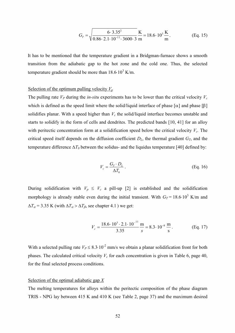
52
m
K106.18
m
K
33600101.286.0
35.36 3
11
2
TG . (Eq. 15)
It has to be mentioned that the temperature gradient in a Bridgman-furnace shows a smooth
transition from the adiabatic gap to the hot zone and the cold one. Thus, the selected
temperature gradient should be more than 18.6103 K/m.
Selection of the optimum pulling velocity Vp
The pulling rate VP during the in-situ experiments has to be lower than the critical velocity Vc
which is defined as the speed limit where the solid/liquid interface of phase [] and phase []
solidifies planar. With a speed higher than Vc the solid/liquid interface becomes unstable and
starts to solidify in the form of cells and dendrites. The predicted bands [10, 41] for an alloy
with peritectic concentration form at a solidification speed below the critical velocity Vc. The
critical speed itself depends on the diffusion coefficient DL, the thermal gradient GT, and the
temperature difference T0 between the solidus- and the liquidus temperature [40] defined by:
0T
DGV LT
c
. (Eq. 16)
During solidification with Vp Vc a pill-up [2] is established and the solidification
morphology is already stable even during the initial transient. With GT = 18.6103 K/m and
T = 3.35 K (with T T, see chapter 4.1) we get:
s
m 103.8
m
35.3
101.2106.18 8
113
s
Vc . (Eq. 17)
With a selected pulling rate VP 8.310-2
mm/s we obtain a planar solidification front for both
phases. The calculated critical velocity Vc for each concentration is given in Table 6, page 40,
for the final selected process conditions.
Selection of the optimal adiabatic gap X
The melting temperatures for alloys within the peritectic composition of the phase diagram
TRIS - NPG lay between 415 K and 410 K (see Table 2, page 37) and the maximum desired

53
temperature for the hot zone is 453 K. To be able to observe the solidification morphology in
the middle of the adiabatic gap, the adiabatic gap is given by:
mm 1.4mm6.18
)415453(2
X
X
TGT . (Eq. 18)
Therefore, the adiabatic gap X should be equal or less than 4.1 mm but wide enough to enable
the observation with a microscope. With the temperature in the hot zone, the calculated length
of the adiabatic zone and the temperature gradient the temperature in the cold zone has to be
377 K.
Summary of possible operation conditions
TRIS is affected by a possible decomposes at high temperature [51, 65]. DSC investigations
show a thermal stability of organic alloys within 4 hours and a temperature of 453 K in the hot
zone. A possible operation window for the in-situ observation is given in Table 8.
Table 8: Possible process conditions for an in-situ observation.
Window for Process Conditions
temperature Thot hot zone Bridgman-furnace 453 K
temperature Tcold in the cold zone of the Bridgman-furnace 377 K
adiabatic gap X (distance between hot and cold zone) 4.15 mm
pulling rate Vp to obtain a planar solidification front 8.310-2
µm/s
maximum experimental time t for Thot = 453 K 4 hours
Despite of all these approximations, the exact range for the in-situ experiments has to be
determined in experiments in the micro Bridgman-furnace itself.

54
4.5 Selected Experimental Procedure
The general experimental procedure is described in the following. The micro Bridgman-
furnace is preheated to bring the entire system, furnace and microscope, in a thermal
equilibrated stage. The selected process conditions are given in Table 9.
Table 9: Selected process conditions for the in-situ observations.
Window for Process Conditions
temperature Thot hot zone Bridgman-furnace 453 K
temperature Tcold in the cold zone of the Bridgman-furnace 353 K
adiabatic gap X (distance between hot and cold zone) 3.6 mm
field of view 636 x 552 or 3180 x 2760 µm2
The sledge which moves the sample through the Bridgman-furnace is at its end position (close
to the hot zone of the Bridgman-furnace). After 1 hour the temperature gradient in the furnace
is stable. The upper plate of the micro Bridgman-furnace is removed and a sample is placed
into the furnace and connected with the sledge. Then the upper plate is put back and the
furnace is closed again. At the beginning, only an empty part of the sample tube is in the hot
zone and the solid material within the capillary tube is approximately 1 mm outside of the hot
plate. That allows the material to expand during melting into the unfilled tube when it is
moved into the hot zone. The whole sample is now moved with relatively high speed
(Vp = 100 mm/s) into the hot zone to the start position of the sledge. Now, the sample is ready
for the solidification experiment, the predefined pulling velocity is set and the DIoS system is
started to record pictures and temperatures. Table 10 shows the number of evaluated
experiments, the prepared concentrations and the applied pulling rates.
Table 10: Implemented experimental setups
VP Concentration in mol fraction
µms 0 0.1 0.2 0.3 0.4 0.45 0.47 0.48 0.5 0.52 0.6 0.7 0.75 0.8 0.9 1
1.28 1 1 1 1 1
1.02 1 1 1 1
0.89 1 1 1 1 2 2 2 1 1 2
0.83 2
0.64 1 2 1 1 1 2 2 1 2 1 1
0.51 1 2 1 1 1 2
0.38 1 2 1 1 2 1 1 1 1 1 2
0.26 1 1 1 1 1 1
0.19 1 2 1 1 2 1 1 1
0.13 2 1 1 2 3 1 3 8 2 1 2 21 1
0.10 1
0.06 1 1 2 2 1 1 1 2 1 1 1 1

55
The stability of the temperature gradient has been evaluated during the solidification
experiments. Two 12 mm long square samples (0.2 x 0.2 mm2) were filled, one with NPG and
one with TRIS. The samples were placed in the two extra slots in the micro Bridgman-furnace
next to the measured sample, see Figure 24 on page 33. During the experiment the two glass
samples stayed unmoved and the position of the phase transition (solid/solid for TRIS and
solid/liquid for NPG) of the pure organic compounds was used to determine the stability of
the temperature gradient.
4.5.1 Experimental Type A: Unmoved Samples
For the stability investigations samples remained immobile in the Bridgman-furnace for
several hours. The DIoS system took every 10 minutes a picture and recorded the
temperatures. A large FOV (3180 x 2760 µm2) was selected to observe most of the entire
adiabatic gap.
4.5.2 Experimental Type B: Moved Samples
The sample was held in the start position at least 30 minutes to prepare a planar solid/liquid
interface. Afterwards, the sample was moved with a constant pulling rate for several hours
through the Bridgman-furnace. The solid/liquid interface morphology was observed with the
DIoS system, taking a picture every 30 or 60 seconds.
To see the entire adiabatic gap, a large FOV was preferred for the first experiments. To see
the microstructures of the solidification morphology in more detail, a small FOV was
preferred for further experiments with the same concentration and the same pulling rate. In a
few cases experiments were started at a certain pulling rate which was then changed during
experiments to a higher, lower or reverse pulling rate to complete the information on the
dynamic of the solidification morphology.
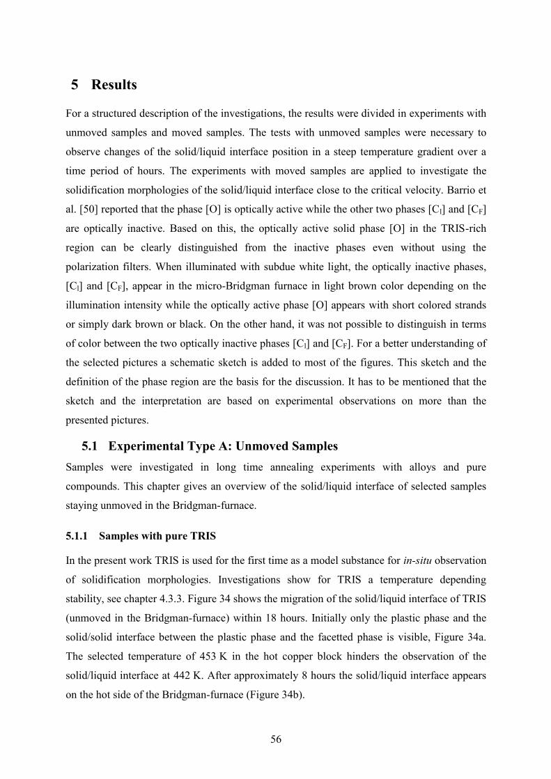
56
5 Results
For a structured description of the investigations, the results were divided in experiments with
unmoved samples and moved samples. The tests with unmoved samples were necessary to
observe changes of the solid/liquid interface position in a steep temperature gradient over a
time period of hours. The experiments with moved samples are applied to investigate the
solidification morphologies of the solid/liquid interface close to the critical velocity. Barrio et
al. [50] reported that the phase [O] is optically active while the other two phases [Cl] and [CF]
are optically inactive. Based on this, the optically active solid phase [O] in the TRIS-rich
region can be clearly distinguished from the inactive phases even without using the
polarization filters. When illuminated with subdue white light, the optically inactive phases,
[Cl] and [CF], appear in the micro-Bridgman furnace in light brown color depending on the
illumination intensity while the optically active phase [O] appears with short colored strands
or simply dark brown or black. On the other hand, it was not possible to distinguish in terms
of color between the two optically inactive phases [Cl] and [CF]. For a better understanding of
the selected pictures a schematic sketch is added to most of the figures. This sketch and the
definition of the phase region are the basis for the discussion. It has to be mentioned that the
sketch and the interpretation are based on experimental observations on more than the
presented pictures.
5.1 Experimental Type A: Unmoved Samples
Samples were investigated in long time annealing experiments with alloys and pure
compounds. This chapter gives an overview of the solid/liquid interface of selected samples
staying unmoved in the Bridgman-furnace.
5.1.1 Samples with pure TRIS
In the present work TRIS is used for the first time as a model substance for in-situ observation
of solidification morphologies. Investigations show for TRIS a temperature depending
stability, see chapter 4.3.3. Figure 34 shows the migration of the solid/liquid interface of TRIS
(unmoved in the Bridgman-furnace) within 18 hours. Initially only the plastic phase and the
solid/solid interface between the plastic phase and the facetted phase is visible, Figure 34a.
The selected temperature of 453 K in the hot copper block hinders the observation of the
solid/liquid interface at 442 K. After approximately 8 hours the solid/liquid interface appears
on the hot side of the Bridgman-furnace (Figure 34b).
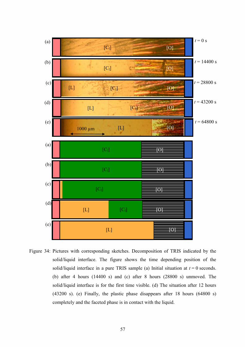
57
Figure 34: Pictures with corresponding sketches. Decomposition of TRIS indicated by the
solid/liquid interface. The figure shows the time depending position of the
solid/liquid interface in a pure TRIS sample (a) Initial situation at t = 0 seconds.
(b) after 4 hours (14400 s) and (c) after 8 hours (28800 s) unmoved. The
solid/liquid interface is for the first time visible. (d) The situation after 12 hours
(43200 s). (e) Finally, the plastic phase disappears after 18 hours (64800 s)
completely and the faceted phase is in contact with the liquid.
t = 64800 s
t = 43200 s
t = 14400 s
t = 28800 s
(a)
(c)
(d)
(e)
[Cl]
[O]
[Cl]
[Cl]
[L]
[L]
[O]
[O]
[L]
[O]
1000 µm
[Cl] (a)
(c)
(d)
[L]
[O]
[Cl]
[O]
[O]
[L] (e)
[O]
[Cl]
[O]
(b)
[O] [Cl]
[Cl] (b)
[O]
t = 0 s

58
During the following 10 hours, the boundary between the liquid and the plastic phase moves
from the left to the right (Figure 34c and d), till the liquid is in contact with the facetted phase
(Figure 34e). Afterwards, the faceted phase starts to dissolve.
However, after cooling and heating-up in the Bridgman-furnace the plastic phase [Cl] and the
facetted phase [O] are re-established again. The sample is kept again unmoved in the furnace
and the plastic phase [Cl] disappears again and the liquid is coming in contact with the faceted
phase [O] after 16 hours.
Figure 35 shows the time depending solid/liquid interface temperatures of the experiments
described above. Both temperature lines are parallel except for the positions were the liquid
phase reached the faceted phase.
0 14400 28800 43200 57600400
405
410
415
420
425
430
435
maximum observation temperature of the applied set-up
Time [s]
1. run solid/liquid interface
2. run solid/liquid interface
faceted phase [O]
pure TRIS
Figure 35: The graph shows the temperature of the solid/liquid interface and the non-
faceted/faceted transition temperature for pure TRIS depending on the
observation time. The plastic phase dissolves with 1.9 ± 0.6 K/h. After 18 hours
the liquid is in contact with the faceted phase.
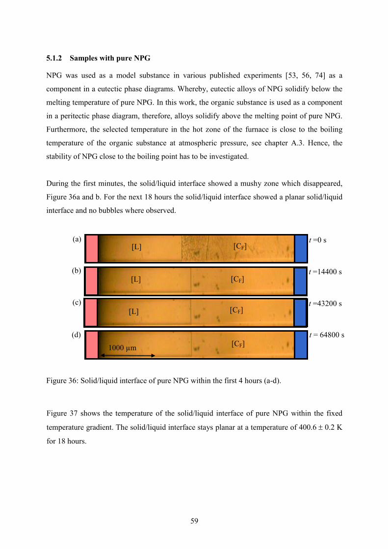
59
5.1.2 Samples with pure NPG
NPG was used as a model substance in various published experiments [53, 56, 74] as a
component in a eutectic phase diagrams. Whereby, eutectic alloys of NPG solidify below the
melting temperature of pure NPG. In this work, the organic substance is used as a component
in a peritectic phase diagram, therefore, alloys solidify above the melting point of pure NPG.
Furthermore, the selected temperature in the hot zone of the furnace is close to the boiling
temperature of the organic substance at atmospheric pressure, see chapter A.3. Hence, the
stability of NPG close to the boiling point has to be investigated.
During the first minutes, the solid/liquid interface showed a mushy zone which disappeared,
Figure 36a and b. For the next 18 hours the solid/liquid interface showed a planar solid/liquid
interface and no bubbles where observed.
Figure 36: Solid/liquid interface of pure NPG within the first 4 hours (a-d).
Figure 37 shows the temperature of the solid/liquid interface of pure NPG within the fixed
temperature gradient. The solid/liquid interface stays planar at a temperature of 400.6 0.2 K
for 18 hours.
t =14400 s
t =43200 s [L] [CF]
(a)
(b)
(c)
[L] [CF]
1000 µm
(d)
[CF]
[CF] [L] t =0 s
t = 64800 s
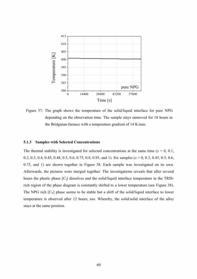
60
0 14400 28800 43200 57600380
385
390
395
400
405
410
415
Time [s]
Tem
per
atu
re [
K]
pure NPG
Figure 37: The graph shows the temperature of the solid/liquid interface for pure NPG
depending on the observation time. The sample stays unmoved for 18 hours in
the Bridgman-furnace with a temperature gradient of 14 K/mm.
5.1.3 Samples with Selected Concentrations
The thermal stability is investigated for selected concentrations at the same time (x = 0, 0.1,
0.2, 0.3, 0.4, 0.45, 0.48, 0.5, 0.6, 0.75, 0.8, 0.95, and 1). Six samples (x = 0, 0.3, 0.45, 0.5, 0.6,
0.75, and 1) are shown together in Figure 38. Each sample was investigated on its own.
Afterwards, the pictures were merged together. The investigations reveals that after several
hours the plastic phase [Cl] dissolves and the solid/liquid interface temperature in the TRIS-
rich region of the phase diagram is constantly shifted to a lower temperature (see Figure 38).
The NPG rich [CF] phase seems to be stable but a shift of the solid/liquid interface to lower
temperature is observed after 12 hours, too. Whereby, the solid/solid interface of the alloy
stays at the same position.

61
Figure 38: Micrographs of stationary samples of various compositions after several hours
within the micro Bridgman setup at a constant temperature gradient. In each
picture the concentration starts at the bottom with x = 0 (TRIS), 0.3, 0.45, 0.5, 0.6,
0.75 and 1 (NPG). The left side shows the pictures and the right side the
interpretation of the phases. (a) Situation after 1 hour within the furnace. (b) Same
samples after 4 hours. (c) Position of the solid/liquid interface after 8 hours
unmoved in the furnace.
(a)
(c)
(b)
[L]
[L]
[L]
[CF] [O] + [CF]
[Cl]
[Cl] + [CF]
[CF]
[CF]
[O]
[O] + [Cl]
[O] + [Cl]
[Cl]
[Cl]
[Cl] + [CF]
[Cl] + [CF]
1000 µm
[O]
[O]
[O] + [CF]

62
The interface temperatures were estimated from the position within the adiabatic gap and the
temperature gradient. In Figure 39 the results of the evaluation of the interface temperatures
after 1 hour have been plotted as points within the phase diagram (as published by Barrio et al
[50]). The points show no error bars because they correspond to single experiments with a
systematic error (measurement error of the temperature and positions) smaller than the point
size. Taking the measurement accuracy into account, the phase transition temperatures
confirm the published phase diagram by Barrio et al. [50].
0.0 0.1 0.2 0.3 0.4 0.5 0.6 0.7 0.8 0.9 1.0
380
390
400
410
420
430
440
450
hyper-peritectic
[CF+O]
[L]
[L+CF]
[L+Cl]
[Cl+O]
[CF+C
l]
[CF]
Tem
per
atu
re [
K]
xTRIS NPG
[Cl]
hypo-peritectic
max. observation temperature of the applied set-up
Figure 39: Comparison of the reported phase diagram [50] (lines with dotted error bands)
with optical investigation (red points) for x = 0, 0.1, 0.2, 0.3, 0.4, 0.45, 0.5, 0.6,
0.75, 0.95 and 1. The maximum temperature observable in the chosen
Bridgman-furnace is shown as a line at 430 K.
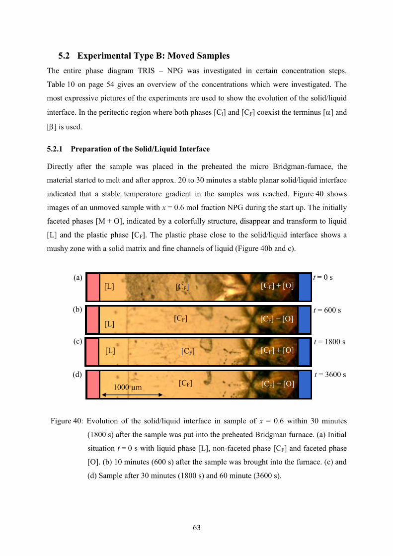
63
5.2 Experimental Type B: Moved Samples
The entire phase diagram TRIS – NPG was investigated in certain concentration steps.
Table 10 on page 54 gives an overview of the concentrations which were investigated. The
most expressive pictures of the experiments are used to show the evolution of the solid/liquid
interface. In the peritectic region where both phases [Cl] and [CF] coexist the terminus [] and
[] is used.
5.2.1 Preparation of the Solid/Liquid Interface
Directly after the sample was placed in the preheated the micro Bridgman-furnace, the
material started to melt and after approx. 20 to 30 minutes a stable planar solid/liquid interface
indicated that a stable temperature gradient in the samples was reached. Figure 40 shows
images of an unmoved sample with x = 0.6 mol fraction NPG during the start up. The initially
faceted phases [M + O], indicated by a colorfully structure, disappear and transform to liquid
[L] and the plastic phase [CF]. The plastic phase close to the solid/liquid interface shows a
mushy zone with a solid matrix and fine channels of liquid (Figure 40b and c).
Figure 40: Evolution of the solid/liquid interface in sample of x = 0.6 within 30 minutes
(1800 s) after the sample was put into the preheated Bridgman furnace. (a) Initial
situation t = 0 s with liquid phase [L], non-faceted phase [CF] and faceted phase
[O]. (b) 10 minutes (600 s) after the sample was brought into the furnace. (c) and
(d) Sample after 30 minutes (1800 s) and 60 minute (3600 s).
[L] [CF]
[CF] + [O]
(a)
(b)
(c)
[L] [CF]
[CF] + [O]
1000 µm
(d) [CF]
[CF] [L] [CF] + [O]
[CF] + [O]
t = 0 s
t = 600 s
t = 1800 s
t = 3600 s

64
Figure 41 shows the temperature of the solid/liquid interface within the first 3600 s from
Figure 40. The interface temperature declined and reached the position which corresponds to
the liquidus temperature within 30 minutes. The mushy zone disappeared and the solid phase
is in equilibrium with the liquid phase.
0 600 1200 1800 2400 3000 3600408
409
410
411
412x = 0.6
T
emp
erat
ure
[K
]
Time [s]
liquidus
temperature
solid/liquid interface
Figure 41: The graph shows the evolution of the solid/liquid interface temperature within the
first hour. The black squares are measurement results with an error of 0.3 K. The
solid/liquid interface reaches a stable liquidus temperature after approximately 30
minutes.
5.2.2 Solidification Morphologies in the [Cl] and the [CF] Phase Region
Solidification morphologies of TRIS at a pulling rate of Vp 0.13 µm/s
For the start-up, the solid/liquid interface stays unmoved during the first 30 minutes and only
the plastic phase [Cl] and the faceted phase [O] is visible, Figure 42a. Afterwards, the sample
was pulled through the Bridgman-furnace with Vp = 0.89 µm/s. During the direct
solidification experiment the organic substance showed initially planar solidification
morphology, see Figure 42b. The solid/liquid interface became unstable and transformed first
to cells and then to dendrites. The low temperature phase grew in the form of facets.
Simultaneously, liquid appeared in front of the faceted phase (Figure 42c) and departs the two
solid phases (plastic phase and faceted phase). The gap of liquid between the faceted phase
and the plastic phase increased until the interdendritic liquid got in contact (Figure 43).

65
Figure 42: Pictures with corresponding sketches of the evolution of the optical solidification
morphology of pure Tris at a pulling rate of Vp = 0.89 µm/s. (a) Initial situation
where only the plastic phase and the faceted phase are visible. (b) TRIS shows a
cellular solid/liquid front on the left side and a straight line for the non-
faceted/faceted transition interface. (c) The initially cellular front becomes
unstable and transforms into dendrites. Simultaneously, the liquid phase appears in
front of the faceted phase and departs both solid phases while the faceted phase
grows in the form of small facets.
The channels and the gap between the faceted phase [O] and the plastic phase [Cl] increased
with time. Finally, the plastic phase somehow appeared in form of small dendrites in front of
the faceted phase until it dissolves and disappears completely.
[Cl] [O] [L]
[L]
[L]
1000 µm
(a)
(b)
(c)
[Cl]
[Cl] [O]
[O]
[L]
[Cl]
(a)
(b)
(c)
[L]
[O]
[O]
[O]
Vp t = 0 s
t = 4710
s
t = 10050 s
[Cl]
[Cl]
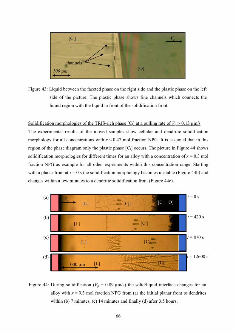
66
Figure 43: Liquid between the faceted phase on the right side and the plastic phase on the left
side of the picture. The plastic phase shows fine channels which connects the
liquid region with the liquid in front of the solidification front.
Solidification morphologies of the TRIS-rich phase [Cl] at a pulling rate of Vp 0.13 µm/s
The experimental results of the moved samples show cellular and dendritic solidification
morphology for all concentrations with x < 0.47 mol fraction NPG. It is assumed that in this
region of the phase diagram only the plastic phase [Cl] occurs. The picture in Figure 44 shows
solidification morphologies for different times for an alloy with a concentration of x = 0.3 mol
fraction NPG as example for all other experiments within this concentration range. Starting
with a planar front at t = 0 s the solidification morphology becomes unstable (Figure 44b) and
changes within a few minutes to a dendritic solidification front (Figure 44c).
Figure 44: During solidification (Vp = 0.89 µm/s) the solid/liquid interface changes for an
alloy with x = 0.3 mol fraction NPG from (a) the initial planar front to dendrites
within (b) 7 minutes, (c) 14 minutes and finally (d) after 3.5 hours.
[Cl]
[O]
[L]
channels
100 µm
Vp
Vp
(a)
(b)
(c)
(d)
[L] [Cl]
[L] [Cl]
[L] [Cl]
[Cl] [L]
[Cl + O]
1000 µm
Vp t = 0 s
t = 420 s
t = 870 s
t = 12600 s

67
It is known from literature that tips of dendrites grow below the liquidus temperature and
above the solidus temperature. Here, a constant shift of the dendrites tips to lower temperature
was always observed in all experiments performed (like Figure 44c and d). Furthermore, the
mushy zone got more extended while the solid/liquid interface moves. In Figure 44d the tip of
the dendrites are 4.7 1 K below the nominal solidus line. Finally, after 10 to 14 hours,
depending on the selected concentration, the entire FOV shows only liquid, therefore, the
solid/liquid interface grows below 353 K.
0 3600 7200 10800408
412
416
420
424
Vp = 0.89*10
-6 m/s
G/V = 1.6*1010
K*s/m2
transformation from planar to dendritic solidification
TS = 418.6 K (DSC measurement)
Tem
per
atu
re [
K]
Time [s]
tip temperature x = 0.3
12
TL = 423.6 K ± 2.5 (DSC measurement)
Figure 45: The graph shows the temperature of the dendrite tips from Figure 44 as a function
of time (x = 0.3 mol fraction NPG and a pulling velocity Vp = 0.89 µm/s). The red
dotted lines show the detected liquidus and solidus temperature by DSC
measurement.
Solidification morphologies of the NPG-rich phase [CF] at a pulling rate of Vp 0.13 µm/s
The solidification morphology of alloys with the NPG-rich [CF] phase, x 0.7 mol fraction,
shows a planar front, before the morphology of the solidification front changes to cells or
dendrites.
Figure 46 shows the solidification morphology of an alloy with x = 0.75 mol fraction NPG
and a pulling velocity of 0.89 µm/s. After more than 4 hours it can be assumed that phases
[CF] grows in steady-state manner because the theoretical transition time is exceeded. The
initial planar front becomes unstable and changes to a cellular solidification morphology.
Note that the cellular solidification front in Figure 46d is undercooled relative to the initial

68
solid/liquid interface in Figure 46a by approximately 3.5 K. The solidification morphology
stays constant even for more than 4 hours.
Figure 46: The solidification morphology of an alloy with x = 0.75 mol fraction NPG and a
pulling velocity of 0.89 µm/s. (a) The initial planar front, (b) the solidification
morphology after 7 minutes, and (c) after 14 minutes and finally (d) cells after
3.5 hours.
Figure 47 shows the temperature of the solid/liquid interface and the cell tips within the first
3.5 hours. During the first 3000 s the position of the planar front moves from the liquidus
temperature close to the solidus temperature. Whereby, the cellular solidification morphology
occurs approximately after the first 1500 s. To a better comparability both graphs in Figure 45
and Figure 47 show the same time and temperature scale. It illustrate that under the same
process conditions the TRIS-rich [Cl] phase dissolve faster than the NPG-rich phase [CF].
Additionally, the [Cl] phase grows dendritic where the [CF] phase grows cellular (compare
Figure 44d and Figure 46d).
(a) [L]
[L]
[L]
[L]
[CF]
[CF]
[CF]
[CF]
(b)
(c)
(d)
1000 µm
Vp t = 0 s
t = 420 s
t = 870 s
t = 12600 s
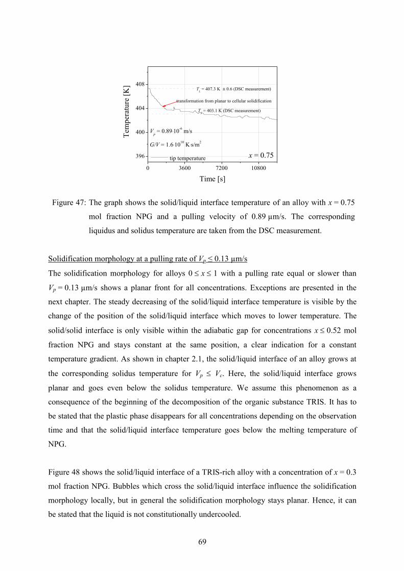
69
0 3600 7200 10800
396
400
404
408
Vp = 0.89·10
-6 m/s
G/V = 1.6·1010
K·s/m2
TS = 403.1 K (DSC measurement)
Tem
per
atu
re [
K]
Time [s]
tip temperature x = 0.75
TL = 407.3 K ± 0.6 (DSC measurement)
transformation from planar to cellular solidification
Figure 47: The graph shows the solid/liquid interface temperature of an alloy with x = 0.75
mol fraction NPG and a pulling velocity of 0.89 µm/s. The corresponding
liquidus and solidus temperature are taken from the DSC measurement.
Solidification morphology at a pulling rate of Vp ≤ 0.13 µm/s
The solidification morphology for alloys 0 x 1 with a pulling rate equal or slower than
Vp = 0.13 µm/s shows a planar front for all concentrations. Exceptions are presented in the
next chapter. The steady decreasing of the solid/liquid interface temperature is visible by the
change of the position of the solid/liquid interface which moves to lower temperature. The
solid/solid interface is only visible within the adiabatic gap for concentrations x 0.52 mol
fraction NPG and stays constant at the same position, a clear indication for a constant
temperature gradient. As shown in chapter 2.1, the solid/liquid interface of an alloy grows at
the corresponding solidus temperature for Vp Vc. Here, the solid/liquid interface grows
planar and goes even below the solidus temperature. We assume this phenomenon as a
consequence of the beginning of the decomposition of the organic substance TRIS. It has to
be stated that the plastic phase disappears for all concentrations depending on the observation
time and that the solid/liquid interface temperature goes below the melting temperature of
NPG.
Figure 48 shows the solid/liquid interface of a TRIS-rich alloy with a concentration of x = 0.3
mol fraction NPG. Bubbles which cross the solid/liquid interface influence the solidification
morphology locally, but in general the solidification morphology stays planar. Hence, it can
be stated that the liquid is not constitutionally undercooled.

70
Figure 48: Solidification morphology of an alloy with x = 0.3 mol fraction NPG and
Vp = 0.13 m/s. The interface shows clearly a planar solid/liquid interface even
when a bubble crosses the solid/liquid interface. The facetted phase can be seen
at the right side.
The evolution of the temperature of the planar solid/liquid interface can be seen in Figure 49.
The graph shows the change of the interface temperature within the first 4 hours. Long time
investigations (t 4 hours) show that the interface stays planar until the plastic phase
disappears completely.
0 3600 7200 10800412
416
420
424
428
TL = 407.3 K (DSC measurement)
TS = 403.1 K (DSC measurement)
x = 0.3
Vp = 0.13*10
-6 m/s
G/V = 1.1*1011
K*s/m2T
emp
erat
ure
[K
]
Time [t]
tip temperature
Figure 49: The morphology of an alloy with x = 0.3 mol fraction NPG solidification occurs
as a planar solid/liquid interface. The graph shows the temperature of the
solid/liquid interface as a function of time, Vp = 0.13 µm/s.
(a)
(b)
(c)
[L]
[L]
[L]
[O] [Cl]
[Cl]
[Cl] 1000 µm
Vp
(d)
t =0 s
t =8940 s
t =14400 s
t =27000 s
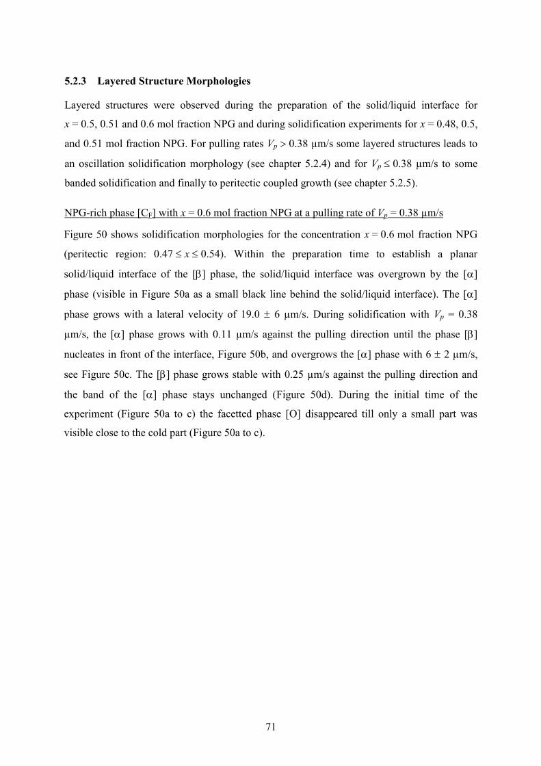
71
5.2.3 Layered Structure Morphologies
Layered structures were observed during the preparation of the solid/liquid interface for
x = 0.5, 0.51 and 0.6 mol fraction NPG and during solidification experiments for x = 0.48, 0.5,
and 0.51 mol fraction NPG. For pulling rates Vp 0.38 µm/s some layered structures leads to
an oscillation solidification morphology (see chapter 5.2.4) and for Vp 0.38 µm/s to some
banded solidification and finally to peritectic coupled growth (see chapter 5.2.5).
NPG-rich phase [CF] with x = 0.6 mol fraction NPG at a pulling rate of Vp = 0.38 µm/s
Figure 50 shows solidification morphologies for the concentration x = 0.6 mol fraction NPG
(peritectic region: 0.47 x 0.54). Within the preparation time to establish a planar
solid/liquid interface of the [] phase, the solid/liquid interface was overgrown by the []
phase (visible in Figure 50a as a small black line behind the solid/liquid interface). The []
phase grows with a lateral velocity of 19.0 6 µm/s. During solidification with Vp = 0.38
µm/s, the [] phase grows with 0.11 µm/s against the pulling direction until the phase []
nucleates in front of the interface, Figure 50b, and overgrows the [] phase with 6 2 µm/s,
see Figure 50c. The [] phase grows stable with 0.25 µm/s against the pulling direction and
the band of the [] phase stays unchanged (Figure 50d). During the initial time of the
experiment (Figure 50a to c) the facetted phase [O] disappeared till only a small part was
visible close to the cold part (Figure 50a to c).
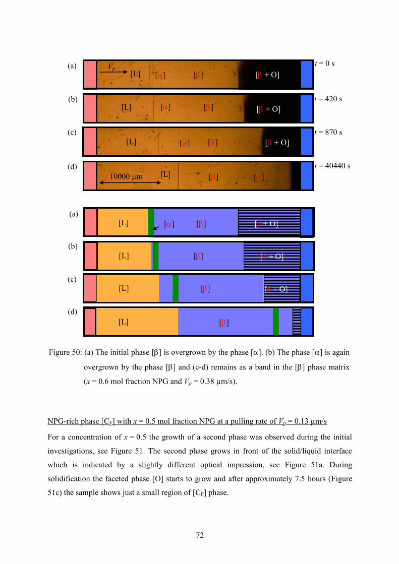
72
Figure 50: (a) The initial phase [] is overgrown by the phase []. (b) The phase [] is again
overgrown by the phase [] and (c-d) remains as a band in the [] phase matrix
(x = 0.6 mol fraction NPG and Vp = 0.38 µm/s).
NPG-rich phase [CF] with x = 0.5 mol fraction NPG at a pulling rate of Vp = 0.13 µm/s
For a concentration of x = 0.5 the growth of a second phase was observed during the initial
investigations, see Figure 51. The second phase grows in front of the solid/liquid interface
which is indicated by a slightly different optical impression, see Figure 51a. During
solidification the faceted phase [O] starts to grow and after approximately 7.5 hours (Figure
51c) the sample shows just a small region of [CF] phase.
[]
[]
(a)
(b)
(c)
(d)
[L] [] []
[L]
[L]
[L]
[]
[]
[]
[]
[]
[]
[ + O]
[ + O]
[ + O]
(a)
(b)
(c)
(d)
[L] [CF] [Cl]
[L]
[L]
[Cl] [CF]
[CF + O]
[CF + O]
[CF + O]
[L]
[]
[ + O]
[ + O]
[ + O]
[L]
[L]
[L]
[]
[]
Vp t = 0 s
t = 420 s
t = 870 s
t = 40440 s
10000 µm
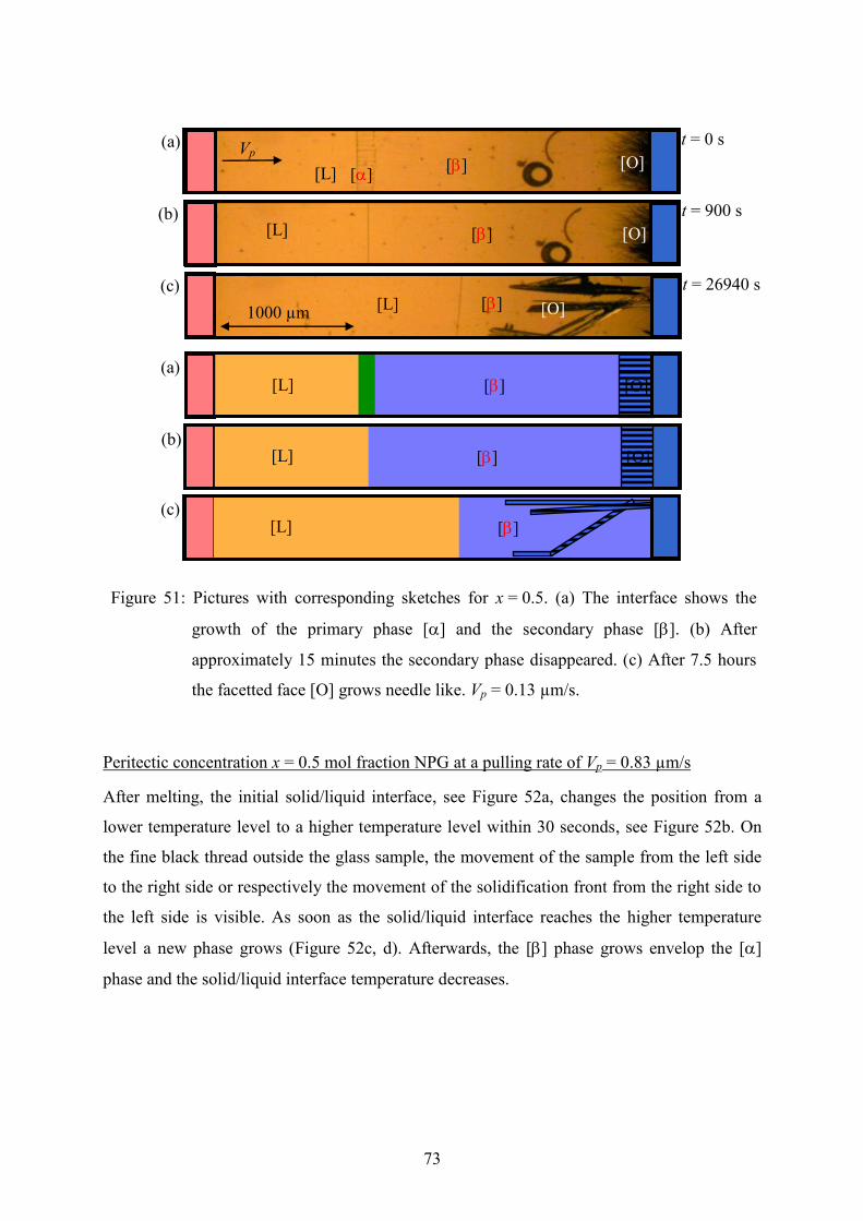
73
Figure 51: Pictures with corresponding sketches for x = 0.5. (a) The interface shows the
growth of the primary phase [] and the secondary phase []. (b) After
approximately 15 minutes the secondary phase disappeared. (c) After 7.5 hours
the facetted face [O] grows needle like. Vp = 0.13 µm/s.
Peritectic concentration x = 0.5 mol fraction NPG at a pulling rate of Vp = 0.83 µm/s
After melting, the initial solid/liquid interface, see Figure 52a, changes the position from a
lower temperature level to a higher temperature level within 30 seconds, see Figure 52b. On
the fine black thread outside the glass sample, the movement of the sample from the left side
to the right side or respectively the movement of the solidification front from the right side to
the left side is visible. As soon as the solid/liquid interface reaches the higher temperature
level a new phase grows (Figure 52c, d). Afterwards, the [] phase grows envelop the []
phase and the solid/liquid interface temperature decreases.
[]
[]
(a)
(b)
(c)
1000 µm
[L]
[L]
[L]
[O]
[O]
[O]
[] []
[]
[]
[L]
[]
[O]
[O]
[L]
[L]
(a)
(b)
(c)
Vp t = 0 s
t = 900 s
t = 26940 s
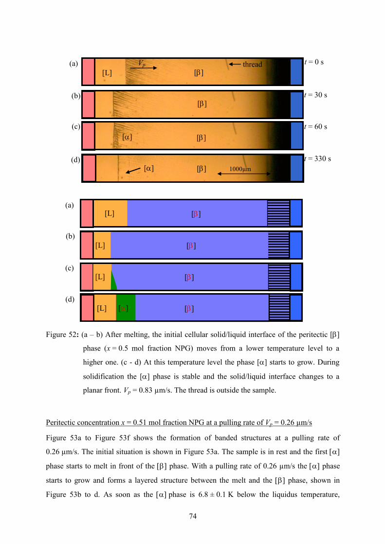
74
Figure 52: (a – b) After melting, the initial cellular solid/liquid interface of the peritectic []
phase (x = 0.5 mol fraction NPG) moves from a lower temperature level to a
higher one. (c - d) At this temperature level the phase [] starts to grow. During
solidification the [] phase is stable and the solid/liquid interface changes to a
planar front. Vp = 0.83 µm/s. The thread is outside the sample.
Peritectic concentration x = 0.51 mol fraction NPG at a pulling rate of Vp = 0.26 µm/s
Figure 53a to Figure 53f shows the formation of banded structures at a pulling rate of
0.26 µm/s. The initial situation is shown in Figure 53a. The sample is in rest and the first
phase starts to melt in front of the phase. With a pulling rate of 0.26 µm/s the phase
starts to grow and forms a layered structure between the melt and the phase, shown in
Figure 53b to d. As soon as the phase is 6.8 ± 0.1 K below the liquidus temperature,
1000µm
(a)
(b)
(c)
(d)
[L] []
[]
[] []
[] []
[]
[]
(a)
(b)
(c)
(d)
[L] [CF] [Cl]
[Cl] [CF]
[CF + O]
[L]
[]
[L]
[L]
[L]
[]
[]
Vp thread t = 0 s
t = 30 s
t = 60 s
t = 330 s
75
TL = 410.06 ± 2.8 K for x = 0.48 mol fraction NPG, the phase starts to grow at a
temperature of 403.5 K. The phase builds a 152 µm broad layer but further phase
transitions or layered structures are not observed.
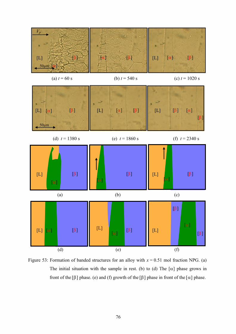
76
(a) t = 60 s (b) t = 540 s (c) t = 1020 s
(d) t = 1380 s (e) t = 1860 s (f) t = 2340 s
(a) (b) (c)
(d) (e) (f)
Figure 53: Formation of banded structures for an alloy with x = 0.51 mol fraction NPG. (a)
The initial situation with the sample in rest. (b) to (d) The [] phase grows in
front of the phase. (e) and (f) growth of the phase in front of the phase.
[]
[] [L] [] [] [] [] [L]
50µm
[] [] [] []
[]
[] [L] [L] [L]
50µm
[]
[] [L] [L] [] [L] []
[] []
[]
[]
[] [L] [L]
[]
[]
[]
[] []
Vp
77
Peritectic concentration x = 0.51 mol fraction NPG at a pulling rate of Vp = 0.19 µm/s
The initial phase [] is expected during the development of a banded solidification structure.
Immediately after the partially melting of the alloy the remaining solid close to the interface
shows a mushy zone, see Figure 54a and in front of the solid/liquid interface there are still
small solid parts.
As soon as the sample is pulled with 0.19 µm/s through the Bridgman-furnace, the coarse
solid/liquid interface tries to create a planar front. During the change of the interface from a
coarse morphology to a planar front the [ phase starts to grow in front of the [] phase.
Figure 54b shows the growth of the [] phase from the outside toward the center of the
sample and simultaneously the [] phase overgrow the [] phase and merge in the center of
the sample (Figure 54c). As soon as the [] phase cuts the [] phase from the liquid, only the
[] phase grows (Figure 54d) and the [] phase forms a lenticular embedding within the []
phase matrix with a thickness of 137 ± 3 µm. After the growth of the [] phase neither a new
solidification of the [] phase in front of the [] phase is observed nor a phase transition from
[] to [] or [] to [], respectively.
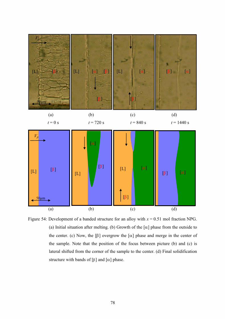
78
(a) (b) (c) (d)
t = 0 s t = 720 s t = 840 s t = 1440 s
(a) (b) (c) (d)
(a) (b) (c) (d)
Figure 54: Development of a banded structure for an alloy with x = 0.51 mol fraction NPG.
(a) Initial situation after melting. (b) Growth of the [] phase from the outside to
the center. (c) Now, the [] overgrow the [] phase and merge in the center of
the sample. Note that the position of the focus between picture (b) and (c) is
lateral shifted from the corner of the sample to the center. (d) Final solidification
structure with bands of [] and [] phase.
[L] [] [] [] [L] [L]
[]
[] []
[]
[]
50µm
Vp
[L] [L]
[L]
50µm
Vp
[] []
[]
[]
[]
[] []

79
To investigate the solidification structure in detail the sample is pulled reverse with 5.11 µm/s
and with that the [] phase starts to melt. The end of the lenticular embedding of the []phase
is observed in Figure 55a together with a melting of [] phase matrix. In addition to [] phase
melting a phase transition from []- to [] was observed in form of small grains which grow
discontinuously, see Figure 55b. Whereby, the [] phase matrix and the grains of the []
phase melted at different temperature levels with T = 0.2 ± 0.05 K Figure 55c).
(a) (b) (c)
t = 0 s t = 18 s t = 33 s
(a) (b) (c)
Figure 55: Melting of the [] phase matrix (x = 0.51 mol fraction NPG). (a) [] phase matrix
with the lenticular embedding [] phase. (b) Phase transition [] to [] within the
[] phase matrix. (c) Different melting temperatures (T) between the [] phase
and the [] phase.
[] [] [] []
[]
[]
[] [] [L]
T
50µm
Vp
Vp [L]
[L] [] []
[]
[] [] []
T

80
5.2.4 Oscillating Morphologies
The solid/liquid interface shows strong oscillations for concentrations of x = 0.5 and 0.6 mol
fraction NPG at a pulling rate of Vp = 0.89 µm/s coupled with a change in morphology from
dendritic to cellular/planar and backwards. In all cases the initial solid/liquid interface was
overgrown by a new phase during the time to establish a planar solid/liquid interface, like in
Figure 50 on page 72.
Oscillating morphology for x = 0.5 mol fraction NPG
An overview of a cycle of an oscillation is shown in Figure 56. The oscillatory growth turned
out to be different from the formation of an alternating sequence of [ and [ bands parallel
to the solidification front. The starting point for the present oscillations is a side-by-side
growth of arrays of []- and []-cells. Both arrays of cells try to form a more or less planar
growth front, until a sudden instability leads to the formation of fine cells of both types, which
are now able to grow faster. Afterwards, the tips thicken again and thus the interface/tip
temperature starts to drop. Close to a “planar” growth of the two cellular arrays the oscillation
starts again. The described mechanism for an oscillatory growth has, to the authors’
knowledge, never been observed before.
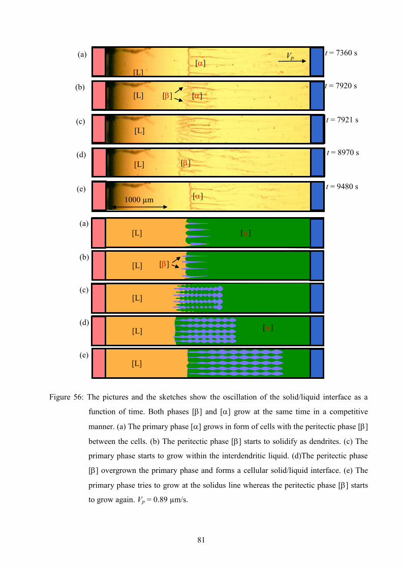
81
Figure 56: The pictures and the sketches show the oscillation of the solid/liquid interface as a
function of time. Both phases [] and [] grow at the same time in a competitive
manner. (a) The primary phase [] grows in form of cells with the peritectic phase []
between the cells. (b) The peritectic phase [] starts to solidify as dendrites. (c) The
primary phase starts to grow within the interdendritic liquid. (d)The peritectic phase
[] overgrown the primary phase and forms a cellular solid/liquid interface. (e) The
primary phase tries to grow at the solidus line whereas the peritectic phase [] starts
to grow again. Vp = 0.89 µm/s.
[L]
[L]
(a)
(c)
(e)
(b)
(d)
[L]
[L]
[L]
[L]
[]
[]
[]
[]
[]
1000 µm
[L]
(a)
(b)
(c)
(d)
[L]
(e)
[L]
[]
[Cl]
Vp
[]
[]
t = 7360 s
t = 7920 s
t = 7921 s
t = 8970 s
t = 9480 s
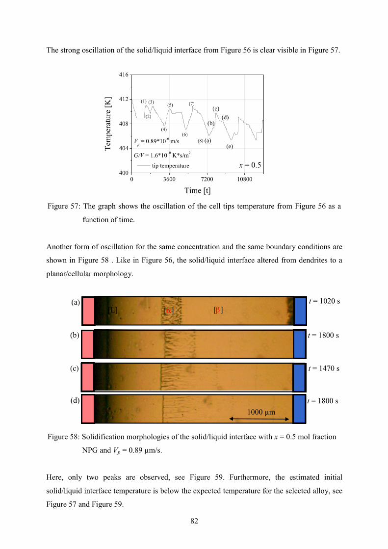
82
The strong oscillation of the solid/liquid interface from Figure 56 is clear visible in Figure 57.
0 3600 7200 10800400
404
408
412
416
Vp = 0.89*10
-6 m/s
G/V = 1.6*1010
K*s/m2
(8)
(7)(5)
(6)(4)
(3)
(2)
(e)
(c)
(a)
(b)(d)
x = 0.5
Tem
per
atu
re [
K]
Time [t]
tip temperature
(1)
Figure 57: The graph shows the oscillation of the cell tips temperature from Figure 56 as a
function of time.
Another form of oscillation for the same concentration and the same boundary conditions are
shown in Figure 58 . Like in Figure 56, the solid/liquid interface altered from dendrites to a
planar/cellular morphology.
Figure 58: Solidification morphologies of the solid/liquid interface with x = 0.5 mol fraction
NPG and Vp = 0.89 µm/s.
Here, only two peaks are observed, see Figure 59. Furthermore, the estimated initial
solid/liquid interface temperature is below the expected temperature for the selected alloy, see
Figure 57 and Figure 59.
(a)
(b)
(c)
(d)
t = 1020 s
t = 1800 s
t = 1470 s
t = 1800 s
[L] [] []
1000 µm
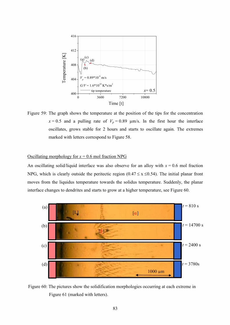
83
0 3600 7200 10800400
404
408
412
416
Vp = 0.89*10
-6 m/s
G/V = 1.6*1010
K*s/m2
(c)
(b)
(d)
x= 0.5
Time [t]
tip temperature
Tem
per
ature
[K
](a)
Figure 59: The graph shows the temperature at the position of the tips for the concentration
x = 0.5 and a pulling rate of Vp = 0.89 µm/s. In the first hour the interface
oscillates, grows stable for 2 hours and starts to oscillate again. The extremes
marked with letters correspond to Figure 58.
Oscillating morphology for x = 0.6 mol fraction NPG
An oscillating solid/liquid interface was also observe for an alloy with x = 0.6 mol fraction
NPG, which is clearly outside the peritectic region (0.47 x 0.54). The initial planar front
moves from the liquidus temperature towards the solidus temperature. Suddenly, the planar
interface changes to dendrites and starts to grow at a higher temperature, see Figure 60.
Figure 60: The pictures show the solidification morphologies occurring at each extreme in
Figure 61 (marked with letters).
(a)
(b)
(c)
(d)
t = 810 s
t = 14700 s
t = 2400 s
t = 3780s
[L] []
[]
1000 µm

84
As soon as the dendrites reached the position at a higher temperature the dendritic solid/liquid
interface decrease again to a lower temperature. From this position the dendrites moves again
forward and grows as dendrites without any further oscillating morphology.
The corresponding temperature of the tip temperature versus time is given in Figure 61. The
oscillation shows only 2 peaks, like in Figure 59, but the form is more like in Figure 57.
0 3600 7200 10800400
402
404
406
408
410
412
414
416
(a)(c)
(d)
Time [t]
T
emp
erat
ure
[K
]
x = 0.6 tip temperature
(b)
Figure 61: The graph shows the temperature of cell/dendrite tips for the alloy with x = 0.6
mol fraction NPG. Compared to the phase diagram, the concentration is clearly
outside of the region where a peritectic reaction or layered structures are expected
(Figure 17 on page 25). The experiment is finished after 3 hours.
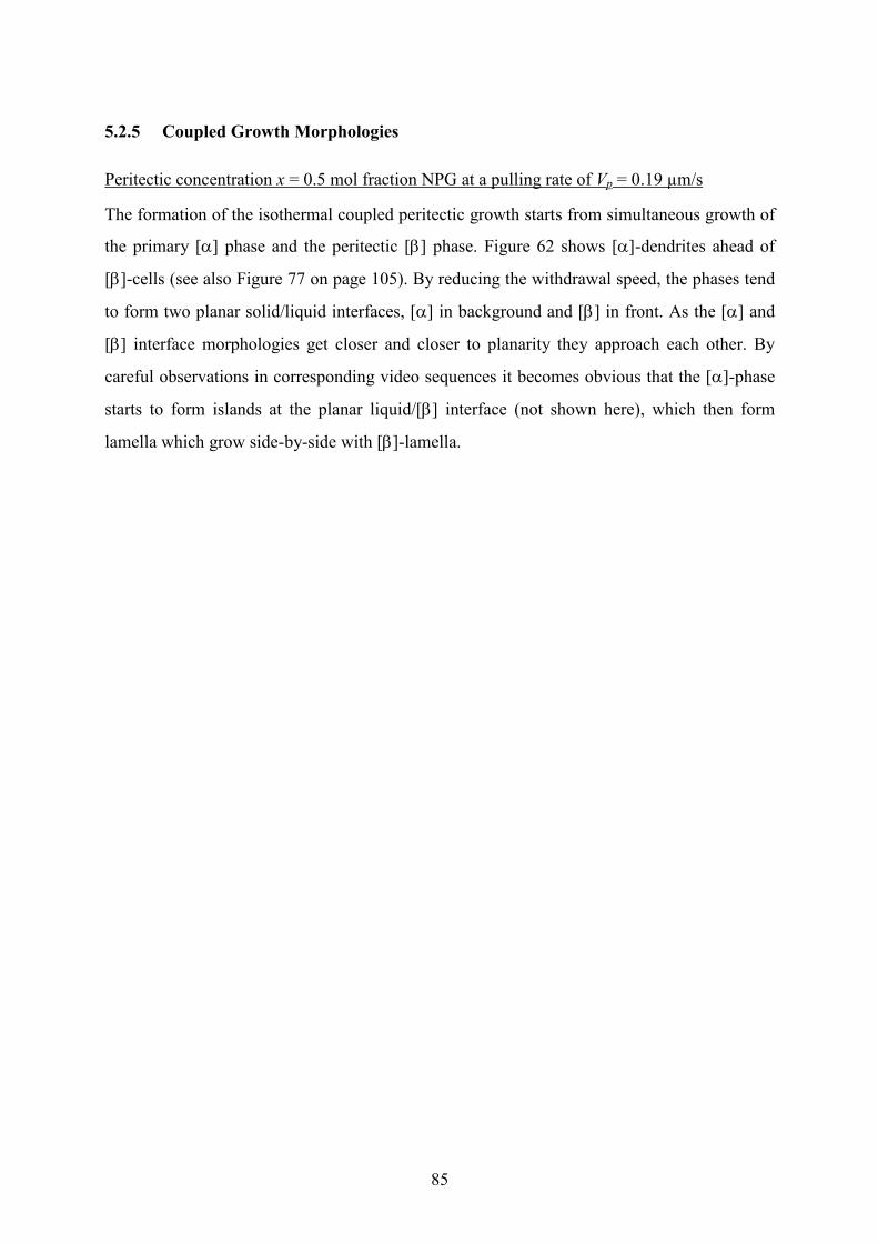
85
5.2.5 Coupled Growth Morphologies
Peritectic concentration x = 0.5 mol fraction NPG at a pulling rate of Vp = 0.19 µm/s
The formation of the isothermal coupled peritectic growth starts from simultaneous growth of
the primary [] phase and the peritectic [] phase. Figure 62 shows []-dendrites ahead of
[]-cells (see also Figure 77 on page 105). By reducing the withdrawal speed, the phases tend
to form two planar solid/liquid interfaces, [] in background and [] in front. As the [] and
[] interface morphologies get closer and closer to planarity they approach each other. By
careful observations in corresponding video sequences it becomes obvious that the []-phase
starts to form islands at the planar liquid/[] interface (not shown here), which then form
lamella which grow side-by-side with []-lamella.
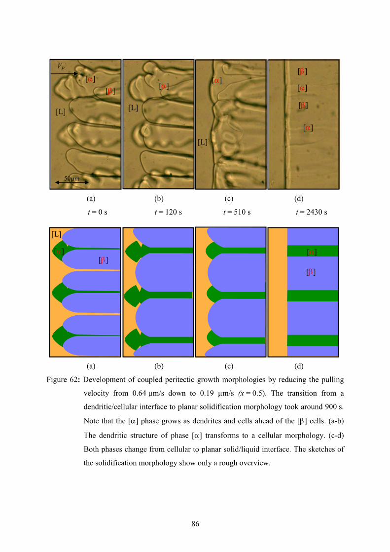
86
(a) (b) (c) (d)
t = 0 s t = 120 s t = 510 s t = 2430 s
(a) (b) (c) (d)
Figure 62: Development of coupled peritectic growth morphologies by reducing the pulling
velocity from 0.64 µm/s down to 0.19 µm/s (x = 0.5). The transition from a
dendritic/cellular interface to planar solidification morphology took around 900 s.
Note that the [] phase grows as dendrites and cells ahead of the [] cells. (a-b)
The dendritic structure of phase [] transforms to a cellular morphology. (c-d)
Both phases change from cellular to planar solid/liquid interface. The sketches of
the solidification morphology show only a rough overview.
[]
[]
[]
[]
[] [] []
[L] [L]
[L]
50µm
Vp
[L]
[] []
[]
[]
[]

87
Peritectic concentration x = 0.51 mol fraction NPG at a pulling rate of Vp = 0.19 µm/s
The solidification morphology with x = 0.51 mol fraction NPG shows a transformation from
banded solidification to coupled growth.
(a) (b) (c) (d)
t = 2400 s t = 2760 s t = 2940 s t = 3240 s
(a) (b) (c) (d)
Figure 63: (a - b) Growth of the [] phase in front of the [] phase (x = 0.51 mol fraction
NPG). (c) The [] phase overgrows the [] phase. (d) Obviously, the [] phase
starts to solidify in front of the solid/liquid interface of the [] phase.
The evolution of the banded structure can be seen in Figure 63. The solid/liquid interface of
the [] phase, was overgrown by the [] phase after 40 minutes after the beginning of the
experiment (Figure 63a and Figure 63b). The [] phase grows laterally from both
solid/liquid/wall junctions of the sample. The entire [] phase was overgrown after
[]
[]
[] []
[] []
[L] [L]
[L]
50µm
[L] []
[] []
[] [] [] []
Vp

88
approximately 10 minutes. The planar solidification front of the [] phase grows stable until
the [] phased nucleates again in front of the solid/liquid interface (Figure 63a, 2 minutes
later).
(a) (b) (c) (d)
t = 4080 s t = 4200 s t = 4800 s t = 9540 s
(a) (b) (c) (d)
Figure 64: Alternating growth of the [] and [] phases and the evolution from banded to
couple growth. The phases are intertwined and the sketches below the pictures
give only a rough overview: (a) growth of solidification bands; (b) nucleation of
the [] phase ahead of the [] phase; (c) lateral growth of the phase leads to a
local undercooling ahead of the phase and to a somewhat chaotic growth
behavior; (d) finally a stable coupled peritectic growth occurs.
The [] phase grows laterally and in solidification direction, as shown in Figure 64a. Since the
[] phase grows at a lower solid/liquid interface temperature compared to the [] phase, the
[] nucleates on various positions in front of the interface of phase [], 15 minutes later as
shown in Figure 64b. The nucleation of the [] phase on various positions ahead of the []
50µm
[] [] [CF]
[]
[]
[]
[]
[L]
T
[]
[]
[]
[]
[]
[L]
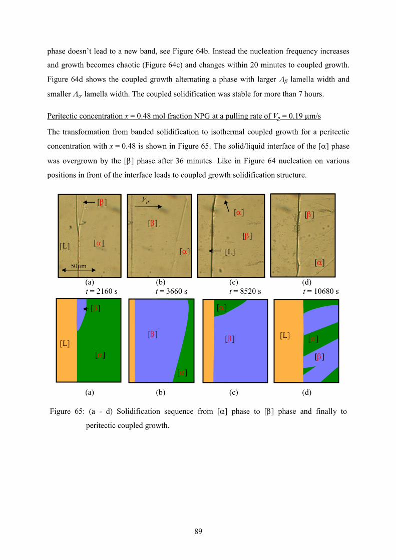
89
phase doesn’t lead to a new band, see Figure 64b. Instead the nucleation frequency increases
and growth becomes chaotic (Figure 64c) and changes within 20 minutes to coupled growth.
Figure 64d shows the coupled growth alternating a phase with larger lamella width and
smaller lamella width. The coupled solidification was stable for more than 7 hours.
Peritectic concentration x = 0.48 mol fraction NPG at a pulling rate of Vp = 0.19 µm/s
The transformation from banded solidification to isothermal coupled growth for a peritectic
concentration with x = 0.48 is shown in Figure 65. The solid/liquid interface of the [] phase
was overgrown by the [] phase after 36 minutes. Like in Figure 64 nucleation on various
positions in front of the interface leads to coupled growth solidification structure.
(a) (b) (c) (d)
t = 2160 s t = 3660 s t = 8520 s t = 10680 s
(a) (b) (c) (d)
Figure 65: (a - d) Solidification sequence from [] phase to [] phase and finally to
peritectic coupled growth.
[]
[]
[]
[]
[]
[] [L] [L]
50µm
[L]
[]
[]
[]
[]
[]
Vp
[]
[]
[]
[]
50µm
[]
[] [L]
[]

90
6 Discussion
During directional solidification of peritectic systems, layered solidification structures are
expected for near peritectic concentrations and solidification rates where the primary and
peritectic phase solidify with a planar solid/liquid interface. Based on the results of the
experiments for the binary organic system TRIS – NPG the expected layered solidification
morphologies were found. Furthermore, the results for this system show a wide range of
layered solidification morphologies and permit a detailed study at how layered solidification
structures occur. Parts of the results are published in [75, 76].
Principally it is not possible to optically distinguish between the primary phase [Cl] and the
peritectic phase [CF]. Therefore, the interpretation of the phases is based on the whole
experimental observation of the entire phase diagram. Additionally, solidification morphology
of the solid/liquid interface close to the critical velocity for [Cl] and [CF] phases are used as a
cross check (see Figure 44 and Figure 46 on page 66 and 68).
6.1 Experimental Type A: Unmoved Samples
6.1.1 Thermal Stability
The thermal stability of the organic substances TRIS and NPG were investigated by DSC
measurements (see chapter 4.3.3.). A thermal stability for 4 hours was detected at the selected
process conditions (see chapter 4.4.1). Nonetheless, the thermal stability of (i) TRIS and NPG
and (ii) selected alloy concentrations were investigated within the constant temperature
gradient. While the sample stayed unmoved within the Bridgman-furnace, the positions of the
phase transitions were recorded.
(i) For TRIS, the selected temperature in the hot zone of the Bridgman-furnace has to be kept
close to the liquidus temperature of TRIS to avoid decomposition [61] (see chapter 4.4.2). As
a consequence, only the plastic phase [Cl], the solid/solid interface and the faceted phase [O]
were visible within the adiabatic gap (see Figure 34a on page 57). The solid/solid transition
interface stayed at a fixed position so that the corresponding interface temperature remains
stable and constant. After 8 hours the solid/liquid interface was visible and another 10 hours
later it reached the solid/solid interface, see Figure 34e. Subsequently, 18 hours after the start
of the experiment the plastic phase [Cl] disappeared totally and the liquid was in direct contact
with the faceted phase [O].

91
The decomposition of the plastic phase [Cl] was measurable by the change of the position of
the solid/liquid interface within the adiabatic zone. The position of the solid/liquid interface
changes by 1.9 ± 0.6 K/h, see Figure 35 on page 58.
After the experiment the sample was removed from the Bridgman-furnace and cooled down to
room temperature. The part of the sample which has been within the hot zone stayed
transparent while the rest of the sample became faceted. The sample was stored at room
temperature, whereby, the transparent part of the sample remains optically unchanged. After
one month the sample was used again for a new non-moving experiment. The transparent part
of the sample was put again into the hot zone of the furnace. The experiment showed the same
behavior as described above. Additionally, the transparent part of the sample was now light
brown and full of small bubbles, properly consisting of TRIS (vaporization), NH3, and H2O,
similar indicating behavior was observed in chapter A.3. The optical investigations of TRIS
confirms the results of the DSC measurements, therefore, TRIS can be used only with great
care.
NPG shows only a small shift of 0.4 ± 0.1 K of the solid/liquid interface during the
solidification experiments within 18 hours, see Figure 37 (page 60). Therefore, NPG can be
used without care at the selected process conditions.
(ii) Selected alloy compositions were prepared in different steps of 10 % to investigate the
entire phase diagram. In the peritectic region additional concentrations are selected. The
solid/liquid interfaces became stable within the first 30 minutes and stay unchanged for the
next hours, see Figure 38a and b on page 61. Approximately after 4 to 5 hours the solid/liquid
interfaces of the [Cl] phase were constantly shifted to lower temperatures. Note that the
observed solid/liquid interface temperature goes even below the solidus temperature. This
effect of decomposition is enhanced for very TRIS-rich concentrations (Figure 38c).
The evolution of the solid/liquid interface temperatures of the pure organic substances and the
alloy with time are shown in Figure 66. The shaded region shows the solid (plastic) phase and
the dots for the solid/liquid interface. Figure 66a shows the situation after 1 hour. The
solid/liquid interface temperatures are approximately at the same level as the temperatures of
the liquidus line of the phase diagram. Within the first 4 hours the solid/liquid interface stayed
fixed (Figure 66b). Afterwards, the decomposition of the TRIS-rich [Cl] phase becomes

92
visible. After 8 hours (Figure 66c), the solid/liquid interface temperature for concentrations of
x ≤ 0.3 is below the solidus temperature of the phase diagram. 12 hours after the beginning of
the experiment the solid/liquid interface temperature for x ≤ 0.5 is below the corresponding
solidus temperature of the phase diagram (Figure 66d).
0.0 0.2 0.4 0.6 0.8 1.0400
410
420
430
440
[Cl]
s/l interface 1 hours
Tem
per
atu
re [
K]
x
[L]
peritectic region
(a)
0.0 0.2 0.4 0.6 0.8 1.0400
410
420
430
440
[Cl]
s/l interface 1 hours
s/l interface 4 hours
Tem
per
atu
re [
K]
x
[L]
peritectic region
(b)
0.0 0.2 0.4 0.6 0.8 1.0400
410
420
430
440
[Cl]
s/l interface 1 hours
s/l interface 4 hours
s/l interface 8 hours
Tem
per
atu
re [
K]
x
[L]
peritectic region
(c)
0.0 0.2 0.4 0.6 0.8 1.0400
410
420
430
440
[Cl]
s/l interface 1 hours
s/l interface 4 hours
s/l interface 8 hours
s/l interface 12 hour
Tem
per
atu
re [
K]
x
[L]
peritectic region
(d)
Figure 66: Effect of the decomposition of TRIS on the solid/liquidus interface within 12
hours. The solid phase is shaded and the solid/liquid interface is shown as blue
dots. (a) Temperature of the solid/liquid interface after 1 hour unmoved in the
temperature gradient. (b) The solid/liquid interface temperatures after 4 hours. (c)
after 8 hours and (d) after 12 hours. The thermal instability of the plastic phase of
TRIS leads to a change of the solid/liquid interface to much lower temperatures
compared to the equilibrium one.
As a consequence of the thermal stability investigations, after 4 hours the solidification
morphologies are no longer used for the interpretation in combination with the phase diagram.
The determination of the microstructure map requires the solidification morphology under
steady state growth conditions. Whereby, solidification morphologies within the peritectic
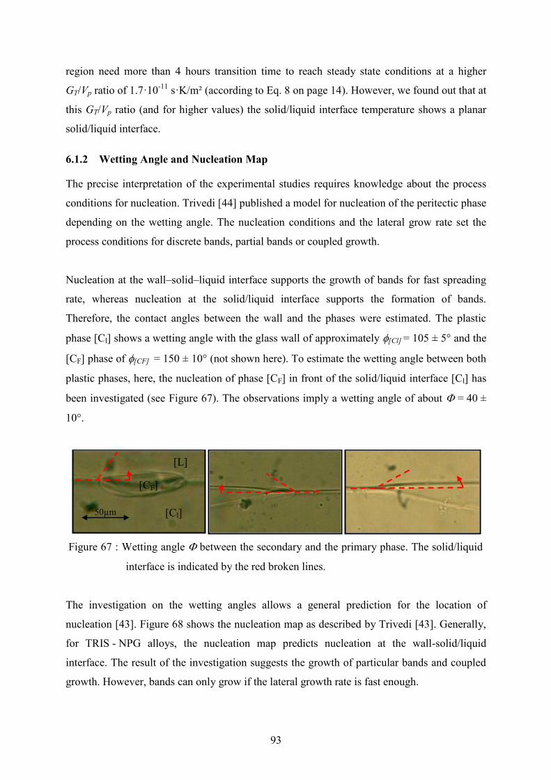
93
region need more than 4 hours transition time to reach steady state conditions at a higher
GT/Vp ratio of 1.7·10-11
s·K/m² (according to Eq. 8 on page 14). However, we found out that at
this GT/Vp ratio (and for higher values) the solid/liquid interface temperature shows a planar
solid/liquid interface.
6.1.2 Wetting Angle and Nucleation Map
The precise interpretation of the experimental studies requires knowledge about the process
conditions for nucleation. Trivedi [44] published a model for nucleation of the peritectic phase
depending on the wetting angle. The nucleation conditions and the lateral grow rate set the
process conditions for discrete bands, partial bands or coupled growth.
Nucleation at the wall–solid–liquid interface supports the growth of bands for fast spreading
rate, whereas nucleation at the solid/liquid interface supports the formation of bands.
Therefore, the contact angles between the wall and the phases were estimated. The plastic
phase [Cl] shows a wetting angle with the glass wall of approximately [Cl] = 105 ± 5° and the
[CF] phase of [CF] = 150 ± 10° (not shown here). To estimate the wetting angle between both
plastic phases, here, the nucleation of phase [CF] in front of the solid/liquid interface [Cl] has
been investigated (see Figure 67). The observations imply a wetting angle of about = 40 ±
10°.
Figure 67 : Wetting angle between the secondary and the primary phase. The solid/liquid
interface is indicated by the red broken lines.
The investigation on the wetting angles allows a general prediction for the location of
nucleation [43]. Figure 68 shows the nucleation map as described by Trivedi [43]. Generally,
for TRIS - NPG alloys, the nucleation map predicts nucleation at the wall-solid/liquid
interface. The result of the investigation suggests the growth of particular bands and coupled
growth. However, bands can only grow if the lateral growth rate is fast enough.
50µm
[L]
[Cl]
[CF]
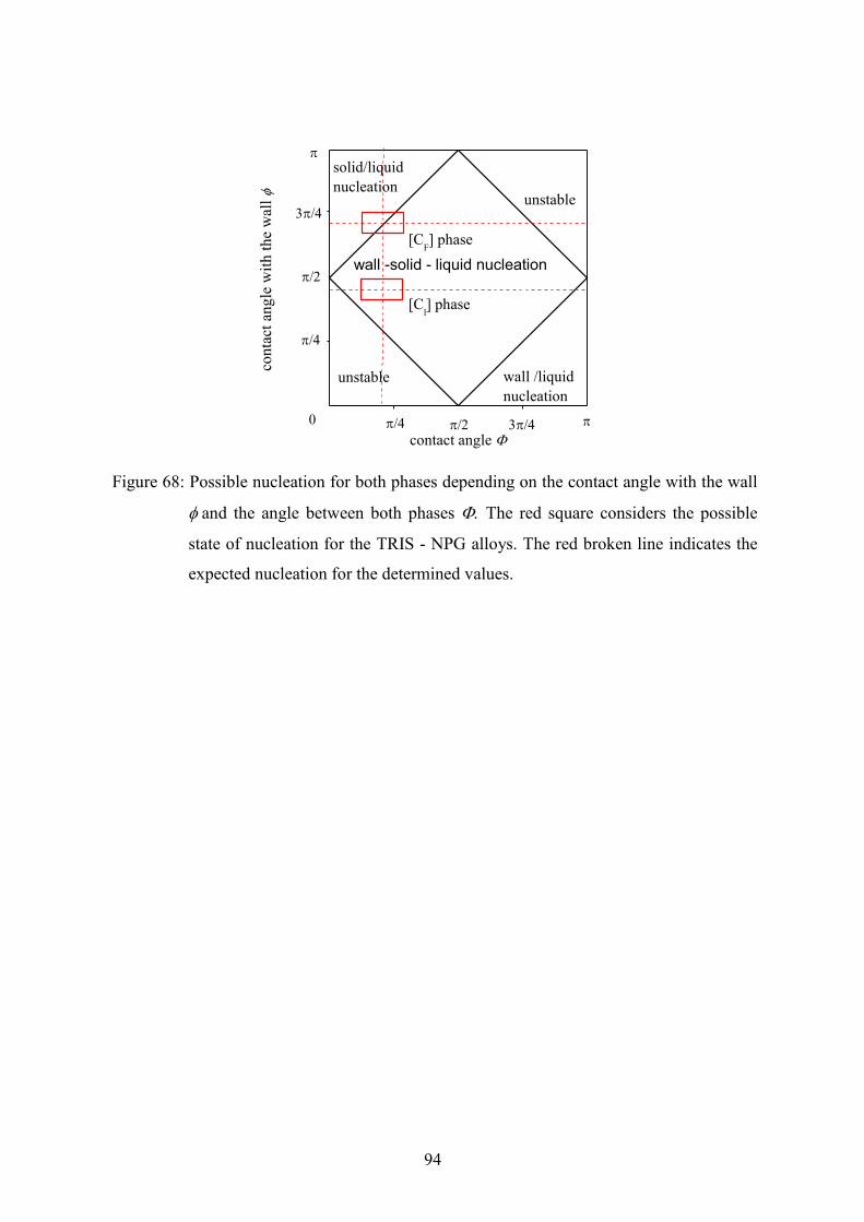
94
[Cl] phase
unstable
unstable
wall /liquid
nucleation
solid/liquid
nucleation
conta
ct a
ngle
wit
h t
he
wal
l
contact angle
wall -solid - liquid nucleation
[CF] phase
Figure 68: Possible nucleation for both phases depending on the contact angle with the wall
and the angle between both phases The red square considers the possible
state of nucleation for the TRIS - NPG alloys. The red broken line indicates the
expected nucleation for the determined values.

95
6.2 Experimental Type B: Moved Samples
6.2.1 Solidification Morphology in the TRIS-rich [Cl] Phase for x ≤ 0.45
For concentrations smaller than x ≤ 0.45 mol fraction NPG (x = 0.1, 0.2, 0.3, 0.4, and 0.45)
and for pulling rates Vp 0.13 µm/s, the initial planar front changes after a certain time into a
dendritic solidification morphology. Figure 44 on page 66 is representative for the
solidification morphology of the [Cl] phase and shows the evolution of the solid/liquid
interface during the solidification experiments for the concentration of x = 0.3 mol fraction
NPG at Vp = 0.89 µm/s within the first 4 hours (see also Figure 45 on page 67).
During the solidification experiments the solid/liquid interface temperature of the planar front
or the cell/dendritic tips changed from the liquidus to the solidus temperature. The solid/liquid
interface transformed from a planar to dendritic solidification morphology close to the solidus
temperature or above. It is expected that the tips of the dendrites are growing at a constant
temperature. Here, the temperature at the dendritic solid/liquid interface decreased constantly
(see Figure 45). This indicates that the plastic phase [Cl] dissolves during solidification
experiments as under the non-moving conditions.
The solidification morphology of samples with a pulling rate of Vp 0.13 µm/s show a planar
solid/liquid front until the plastic phase disappears (t 4 hours). At this point the facetted
phase gets in contact with the liquid, see Figure 48 on page 70.
6.2.2 Solidification Morphology in the NPG-rich [CF] Phase for x > 0.6
The solidification morphology of alloys with x > 0.6 mol fraction NPG (x = 0.7, 0.75, 0.8,
0.85, 0.9, and 0.95) and for pulling rates Vp 0.13 µm/s were investigated. The solid/liquid
interface grows planar until the interface reached a temperature close to the solidus
temperature or even lower. In contrast to the dendritic solidification morphology in the [Cl]
phase, here the [CF] phase solidified cellular (Figure 46 on page 68). The cell tip temperature
of the [CF] phase decreases below the solidus temperature and for very long time
investigations (t > 24 hours) even below the melting point of pure NPG.
Like the solidification morphology of the [Cl] phase the solid/liquid interface of the [CF]
phase solidify in a planar manner at a pulling rate of Vp 0.13 µm/s.
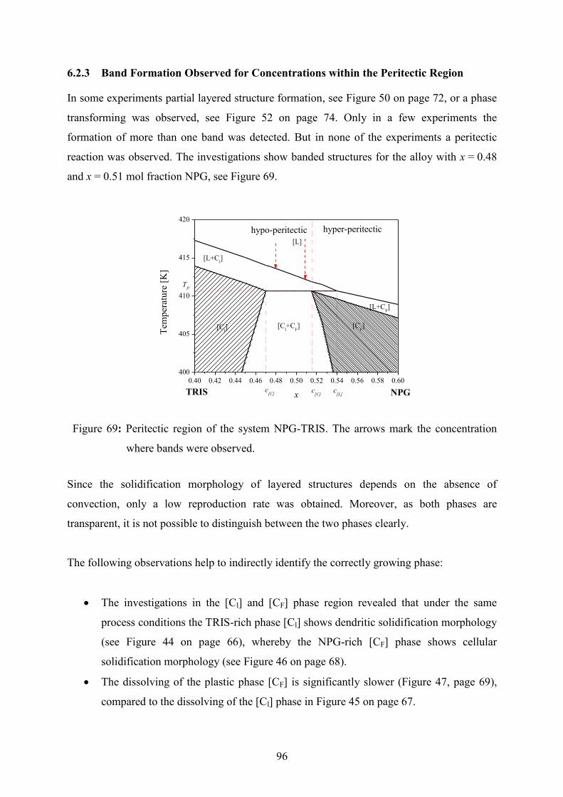
96
6.2.3 Band Formation Observed for Concentrations within the Peritectic Region
In some experiments partial layered structure formation, see Figure 50 on page 72, or a phase
transforming was observed, see Figure 52 on page 74. Only in a few experiments the
formation of more than one band was detected. But in none of the experiments a peritectic
reaction was observed. The investigations show banded structures for the alloy with x = 0.48
and x = 0.51 mol fraction NPG, see Figure 69.
0.40 0.42 0.44 0.46 0.48 0.50 0.52 0.54 0.56 0.58 0.60
400
405
410
415
420
TP
c[L]
c[C] NPGTRIS
[CF][C
l+C
F][C
l]
[L+CF]
[L]
[L+Cl]
c[C]
hypo-peritectic hyper-peritectic
Tem
per
atu
re [
K]
x
Figure 69: Peritectic region of the system NPG-TRIS. The arrows mark the concentration
where bands were observed.
Since the solidification morphology of layered structures depends on the absence of
convection, only a low reproduction rate was obtained. Moreover, as both phases are
transparent, it is not possible to distinguish between the two phases clearly.
The following observations help to indirectly identify the correctly growing phase:
The investigations in the [Cl] and [CF] phase region revealed that under the same
process conditions the TRIS-rich phase [Cl] shows dendritic solidification morphology
(see Figure 44 on page 66), whereby the NPG-rich [CF] phase shows cellular
solidification morphology (see Figure 46 on page 68).
The dissolving of the plastic phase [CF] is significantly slower (Figure 47, page 69),
compared to the dissolving of the [Cl] phase in Figure 45 on page 67.

97
Furthermore, it is assumed that, independently from the initially growing phase, the
phase that grows corresponds finally to the phase diagram.
Banded growth requires an oscillating planar solid/liquid interface due to the differently in the
liquidus temperatures of the [Cl] and [CF] phases (see Figure 11 on page 17). The solid/liquid
interface of the primary [Cl] phase prefers to grow at the [Cl] solidus temperature which is at a
lower temperature compared to the [CF] one. The movement is in pulling direction, therefore,
the solidification velocity of the solid/liquid interface increases. The opposite applies for the
peritectic phase [CF] which is undercooled in respect to the primary phase [Cl]. As soon as the
peritectic phase [CF] starts to solidify it prefers to grow at the solidus temperature of the [CF]
phase which is at a higher temperatures. Thus, the solid/liquid interface grows against the
pulling direction and the solidification velocity decreases. Therefore, during banded
solidification the growth velocity of the planar solid/liquid interface with respect to the
pulling velocity helps to indicate the correct phases.
Under this assumption, the determination of the [Cl] and [CF] phase during lateral growth in
chapter 5.2.5 is possible. Table 11 shows the growth velocity (parallel to the solidification
direction for both plastic phases) compared to the pulling rate VP.
Table 11: Comparison of the growth rate and the pulling rate VP for x = 0.48 and x = 0.51.
x Vp [] error [] error
µm/s µm/s µm/s µm/s µm/s
0.48 0.19 0.21 0.03 0.13 0.03
0.51 0.19 0.21 0.03 0.14 0.03
0.51 0.19 0.21 0.04 0.18 0.02
The [] phase is indicated as the [Cl] phase because the solid/liquid interface of the [] phase
moves faster than the selected pulling rate. Consequently, the [] phase is the peritectic [CF]
phase.
The calculation of the expected lamella distances requires the knowledge of the undercooling
TN of both phases which is due to the constant shift of the solid/liquid interface
experimentally not determinable. For an alloy of x = 0.51 mol fraction NPG it is only possible
to measure the width of two bands, namely which is 76 10 µm for the [CF] phase and 190
10 µm for the [Cl] phase. These values agree with equation 10 and 11 (see chapter 2.1.2) if the
following nucleation undercooling is chosen: TNCl
= 0.12 K and TNCF
= 0.44 K.

98
6.2.4 Oscillation Observed for Concentrations within the Peritectic Region and slightly
above
As described in chapter 5.2.4 oscillating solidification morphologies are observed for
concentrations of x = 0.5 and 0.6 mol fraction NPG for Vp Vc. Note, that the oscillatory
growth, as described here, is different from the formation of an alternating sequence of [Cl]
and [CF] bands parallel to the solidification front (banded microstructures) where alternative
bands grow at velocities below the limit of constitutional undercooling (planar front growth),
whereas here the growth velocity is definitely larger.
The oscillations discussed in this section occur for growth velocities above the limit of
constitutional undercooling. To discuss this oscillating solidification event we refer to the
observations for x = 0.6 mol fraction, presented in Figure 60 and Figure 61 on page 83.
Detailed investigation shows the nucleation of the [CF] phase. The initial planar solid/liquid
interface of the [Cl] phase became unstable. Within the perturbations of the solid/liquid
interfaces the [CF] phase nucleated. The new phase [CF] (red circles) differs from the
perturbations of the existing phase [Cl] (blue circles) by a solid/solid interface, visible as a
small black line, see Figure 70. Both phases start to grow but only the dendrites of the [Cl]
phase overgrow the [CF] phase.

99
Figure 70: The figure shows the solid/liquid interface of x = 0.6 mol fraction NPG in detail.
(a - b) The interface becomes instable. Parts of the interface show instability
(blue circle) where other parts show the nucleation of the primary [CF] phase (red
circle). (c) The [CF] phase becomes partly overgrown by the [Cl] phase.
Figure 61 (page 84) shows the oscillation of the solid/liquid interface within first hours for
x = 0.6 mol fraction NPG. The dendritic interface oscillated with a 15 minutes cycle. After
one hour of oscillation the solidification front grows as dendrites. The growth of dendrites
under the present conditions identifies the grow phase as the [Cl] phase. It has to be noted, that
in other cases when no oscillation solidification was observed (under the same boundary
conditions) the solidification morphology shows instead a cellular interface.
For an alloy with x = 0.5 mol fraction NPG different strong oscillations were observed. In
Figure 59 (page 83) the oscillation shows only two cycles. Remarkable is the change from the
initial solidification temperature at 408 K to a higher solid/liquid interface close to 409 K.
(a)
(b)
t =510 s
t =720 s
t =990 s
80µm
100
In Figure 57 on page 82 the oscillation shows 7 peaks during more than 4 hours. One
oscillation time period is approximately 2109 ± 169 s and the alloy solidifies over a length of
1.89 ± 0.15 mm. The time period and the width of one period remain constant in this
experiment. Originally started with the present of a band and a planar solid/liquid interface,
the solidification morphology changes its morphology from a dendritic front to dendrites with
a higher growth velocity. The dendrites grow against the pulling direction until the
interdendritic liquid starts to solidify. Meanwhile the dendrite tips reach the maximum
temperature and the tip radius increases. Now the solidification stops and the dendrites
transform to cells and to a cellular/planar front which falls back to lower temperature until the
oscillation starts again.
Unfortunately, the increasing undercooling of the TRIS-rich [Cl] phase over time makes it
difficult to compare the results of these investigations with the phase diagram. The first
observed dendrites grow below the peritectic temperature and the following cycle of the
oscillation grows at an even lower temperature.
Since this oscillatory solidification sequence has never been reported before, the oscillation
from Figure 57 is described in more details in Figure 71 to Figure 77. The following facts
limit the interpretation of the observation. Both plastic phases are transparent, therefore, it is
not possible to distinguish the two phases optically. Published and measured errors of the
liquidus and solidus temperature are close to the temperature difference between solidus and
liquidus line. Furthermore, the TRIS-rich phase tends to decompose slightly with time.
Two ways of interpretations for the oscillating morphology are given: (i) competitive growth
of both phases in comparison to the modified phase diagram and (ii) oscillation as a
consequence of the solutal layer in front of the leading phase.
Competitive growth of both phases explained by the modified phase diagram
The assumption of a competition in growth of both phases, in comparison with the phase
diagram, considers the fact that the solidus and liquidus line of both phases, [Cl] and [CF],
decrease in each cycle. Figure 71 shows the modification of the solidus and liquidus line after
1800 s.

101
0.40 0.45 0.50 0.55 0.60 0.65
406
408
410
412
414
[Cl] solidus line
[CF] liquidus line
T
emper
ature
[K
]
x
[Cl] liquidus line
[CF] solidus line
0.40 0.45 0.50 0.55 0.60 0.65
406
408
410
412
414
[Cl] solidus line
[Cl] liquidus line
[CF] liquidus line
Tem
per
ature
[K
]
x
[CF] solidus line
Figure 71: The graph shows a possible variation of the solidus and liquidus line to lower
temperatures during solidification experiments as a consequence of the
decomposition of TRIS.
Figure 73 covers the time period from the peak 3 to peak 6 as defined in Figure 57. From peak
3 to peak 6 the corresponding concentration of each cycle is given in the phase diagram, see
Figure 72.
The explanation starts with the situation in peak 3 in Figure 57 on page 82. The solid/liquid
interfaces of both phases ([Cl] and [CF]) follow the solidus line and try to reach a stable planar
front (see Figure 72a, red broken arrow 1 for phase [Cl]) Now, the solid/liquid interface is
constitutional undercooled and changes its morphology from a cellular/planar front (like
Figure 73a) to shallow cells and dendrites (like Figure 73b). This change of the solidification
morphology is equal to the arrow 2 and 3 in Figure 72b. The dendrite tips grow against the
pulling direction, see Figure 72 red broken arrow 3, to reach equilibrium at the initial
concentration of x = 0.5 mol fraction NPG. The shallow [CF] cells changes to deep cells and
grow behind the [Cl] dendrites.
Shortly afterwards, the concentration in the liquid reaches the concentration where the
peritectic phase [CF] can grow and the intercellular liquid again solidifies (compare Figure
73c-d). Now, both phases grow isothermally (see arrow 5 in Figure 72c). As soon as the
dendrite tips of the [Cl] and [CF] phase reach the maximum temperature the tip radii increase
(Figure 73e - f). The morphology changes from dendrites to a cellular/planar front (see Figure
72 red broken arrow 6). The dendrites transform to cells (Figure 73i) and both phases then to a
cellular/planar front (Figure 73j). The solid/liquid interface temperature increases, see Figure
72 red broken arrow 7 and 8. Afterwards, the solidification cycle starts again.

102
0.40 0.45 0.50 0.55 0.60 0.65
406
408
410
412
414
[Cl] solidus line
[CF] liquidus line
Tem
per
ature
[K
]
x
1
[Cl] liquidus line
[CF] solidus line
(a)
0.40 0.45 0.50 0.55 0.60 0.65
406
408
410
412
414
[Cl] solidus line
[CF] liquidus line
Tem
per
atu
re [
K]
x
3
2
[Cl] liquidus line
[CF] solidus line
(b)
0.40 0.45 0.50 0.55 0.60 0.65
406
408
410
412
414
[Cl] solidus line
[CF] liquidus line
Tem
per
ature
[K
]
x
5
[Cl] liquidus line
[CF] solidus line
4
(c)
0.40 0.45 0.50 0.55 0.60 0.65
406
408
410
412
414
[Cl] solidus line
[CF] liquidus line
Tem
per
ature
[K
]
x
6
7
[Cl] liquidus line
[CF] solidus line
8
(d)
Figure 72: Cooperative oscillation growth of both phases from the peaks 3 to 6 as defined in
Figure 57, whereby in each oscillation cycle the solidus and liquidus line
decrease. (a) The [Cl] phase (red dots) starts to grow as a nearly planar front
along the [Cl] solidus line (arrow 1). (b) Close to the final concentration the
planar front becomes unstable (arrow 2) and grows as a dendritic [Cl] and
cellular [CF] solidification front back to the initial concentration (arrow 3). (c)
Close to the initial concentration the undercooling in the interdendritic liquid is
sufficient so that the peritectic phase [CF] (black dots) can grow (arrow 4) in
addition to the primary phase [Cl] (arrow 5). (d) Both phases try to grow as a
planar front (arrow 6 – 8) and the loop starts again.
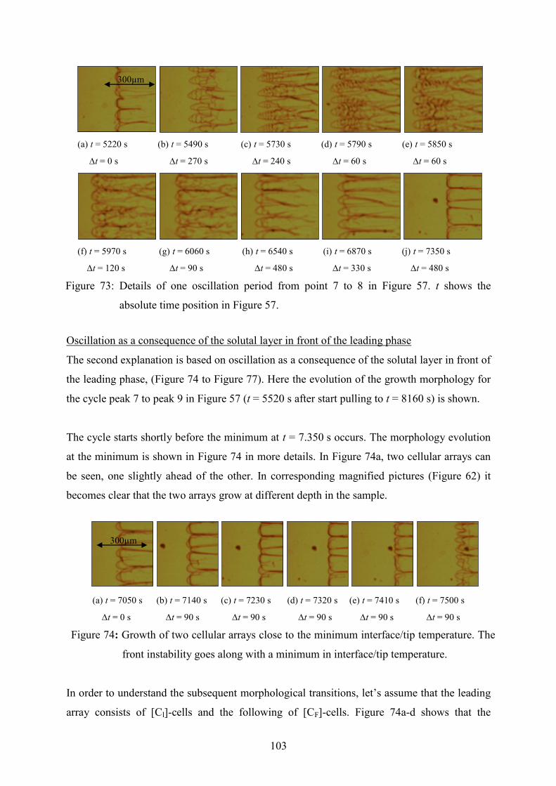
103
(a) t = 5220 s (b) t = 5490 s (c) t = 5730 s (d) t = 5790 s (e) t = 5850 s
t = 0 s t = 270 s t = 240 s t = 60 s t = 60 s
(f) t = 5970 s (g) t = 6060 s (h) t = 6540 s (i) t = 6870 s (j) t = 7350 s
t = 120 s t = 90 s t = 480 s t = 330 s t = 480 s
Figure 73: Details of one oscillation period from point 7 to 8 in Figure 57. t shows the
absolute time position in Figure 57.
Oscillation as a consequence of the solutal layer in front of the leading phase
The second explanation is based on oscillation as a consequence of the solutal layer in front of
the leading phase, (Figure 74 to Figure 77). Here the evolution of the growth morphology for
the cycle peak 7 to peak 9 in Figure 57 (t = 5520 s after start pulling to t = 8160 s) is shown.
The cycle starts shortly before the minimum at t = 7.350 s occurs. The morphology evolution
at the minimum is shown in Figure 74 in more details. In Figure 74a, two cellular arrays can
be seen, one slightly ahead of the other. In corresponding magnified pictures (Figure 62) it
becomes clear that the two arrays grow at different depth in the sample.
(a) t = 7050 s (b) t = 7140 s (c) t = 7230 s (d) t = 7320 s (e) t = 7410 s (f) t = 7500 s
t = 0 s t = 90 s t = 90 s t = 90 s t = 90 s t = 90 s
Figure 74: Growth of two cellular arrays close to the minimum interface/tip temperature. The
front instability goes along with a minimum in interface/tip temperature.
In order to understand the subsequent morphological transitions, let’s assume that the leading
array consists of [Cl]-cells and the following of [CF]-cells. Figure 74a-d shows that the
300µm
300µm

104
advance of the [Cl]-cells gradually disappears until both cellular arrays grow with the same
interface temperature. However, this “side-by side” growth is obviously inherently unstable
and leads to a sudden advance of smaller cells of both phases. Careful observation of
morphological details makes it obvious that after the advance of the small cells of both phases
the [Cl]-cells once more move ahead of the [CF]-cells (see Figure 75).
(a) t = 7380 s (b) t = 7440 s (c) t = 7500 s (d) t = 7560 s (e) t = 7620 s (f) t = 7680 s
(g) t = 7740 s (h) t = 7800 s (i) t = 7860 s (j) t = 7920 s (k) t = 7980 s (l) t = 8040 s
Figure 75: Two examples which show that after new finer cells of both phases occur, the
fine [Cl]-cells are leading against the fine [CF]-cells. In pictures (f) and (l) [Cl] is
again the leading phase. The pictures are taken at t = 7.380 s after starting
pulling with a time increment of Δt = 60 s.
The leading fine [Cl]-cells further develop into dendrites, as can be seen in Figure 76a. These
isolated dendrites grow clearly ahead of the cellular front which might now consist mostly of
[CF]-cells. One might expect that the [Cl]-dendrites now gradually try to reach steady-state.
Suddenly all growing objects, [Cl]-dendrites and [CF]-cells, shot forwards, as shown in Figure
76b - d. This can be understood by considering the fact that a flat growth front which consists
of deep cells (as shown in Figure 75) does have a large solute layer = 2·D/V similar to a
planar front. After the sudden occurrence of the fine cellular growth, these cells have to grow
right into the solute boundary layer. With Vp = 0.89 µm/s and DL = 2.010-11
m2/s for x = 0.5
mol fraction NPG (see chapter 4.1) the boundary layer can be calculated to be = 45 µm in
thickness, 2 times smaller as the observed growth length. The weakness here is that the exact
solute boundary layer of each phase is unknown. Due to the fact that the tip radius of the fine
cells is much smaller than that of the former larger cells, the corresponding growth diffusion
field is more or less localized around the tips. Therefore, the growth velocity can increase for
both, the leading [Cl]-cells/dendrites as well as the following [CF]-cells. This leads to a
300µm

105
gradual forward motion of the front until the front reaches the end of the boundary layer.
Here, the corresponding tips feel the initial melt composition and can further accelerate until
they reach a temperature close to the related steady-state tip temperature for the fast growth.
(a) t = 7890 s (b) t = 7920 s (c) t = 7950 s (d) t = 7980 s (e) t = 8010 s (f) t = 8040 s
Figure 76: The leading [Cl]-dendrites as well as the following [CF]-cells advance gradually
until they reach the end of the solute boundary layer which has been formed
previously. Feeling the initial melt concentration further acceleration of the tips
occur until the tip temperatures are close to the related steady-state tip
temperature for the fast growth. Then the tip velocity adapts to the pulling speed
and tip thickening occurs. The pictures are taken t = 7.890 s after starting pulling
with a time increment of Δt = 30 s.
However, now the tips have to adapt to the pulling speed, therefore, the tip radii gets larger
and larger (Figure 76d - f). Note that the [Cl]- and [CF]-tips do thicken at slightly different
temperatures. The reason for that is that due to the higher liquidus temperature of [Cl],
compared to [CF], and due to an approximately similar tip undercooling, the tip temperature of
[Cl] is higher than that of [CF]. This argument confirms that the assumption of [Cl] being the
leading phase is reasonable. It is important to notice that as soon as the tips adapt to the
pulling velocity, the maximum of the interface/tip temperature cycle is reached.
(a) t = 8040 s (b) t = 8070 s (c) t = 8100 s (d) t = 8130 s (e) t = 8160 s
Figure 77: After reducing the growth velocity in order to adapt the pulling speed, tip
thickening results in a transition from dendrite-like into cell-like growth. With
that the interface/tip temperature decreases. Note that the [Cl]-cells/dendrites
keep being ahead of the subsequently [CF]-cells. The pictures are taken with a
time increment of Δt = 30 s.
300µm
300µm
106
With the following tip thickening (see Figure 76e - f) a change from isolated-tip-growth to a
diffusion-field-overlapping-growth occurs. In consequence the tip temperatures decrease
again. The difference in tip temperatures between the [Cl]-cells and [CF]-cells remains, while
the interface/tip temperature further drops. Figure 77 shows the evolution of the interface
morphology from the maximum of the interface/tip temperature to its minimum. Note that
Figure 77e, taken at the end of the corresponding cycle, is similar to Figure 73a, which
represent the beginning of the cycle.
The solidification morphology shows that the oscillation occurs at a GT/Vp ratio where both
phases solidify not planar (above the limit of constitutional undercooling). In this region the
primary phase [Cl] solidifies as dendrites where the secondary phase [CF] forms cells
(Vp = 0.89 µm/s), therefore, they did not accomplish the assumptions for layered structure
formation formulated in [50]. Nucleation is unnecessary because already both phases are
present and solidify in a competitive manner.
6.2.5 Isothermal Coupled Growth Observed for Concentrations within the Peritectic
Region
Isothermal peritectic coupled growth (PCG) was discussed in literature and experimental
evidences were found in [17, 22, 26, 27]. Additionally, simulation shows a wide range of
different solidification within the peritectic region [26]. In this thesis, isothermal peritectic
coupled growth (PCG) is observed for alloys with x = 0.48, 0.50 and 0.51 mol fraction NPG.
Within the hypo-peritectic region, see Figure 4 on page 9, close to the [C] concentration, the
peritectic [] phase solidifies in form of islands within the primary [] phase. Whereby, in the
hyper-peritectic region close to the [C] concentration the primary [] phase is imbedded in
the peritectic [] phase. In between, both phases solidify in a lamella form, like eutectic
coupled growth.
In the present thesis, PCG was reached under two different conditions (i) by long-time
growing with a constant velocity below the critical value for morphological stability of both
solid phases, or by (ii) reducing the growth velocity from above the critical value for
morphological stability of both solid phases to a value below the limit of constitutional
undercooling. In both cases island banding was observed, where nucleation and lateral growth
of the peritectic phase compete with growth of the primary phase. Interphase spacing and the

107
widths of [α] and [β] lamellae were measured as function of growth velocity for a fixed
composition and as function of composition for a fix growth velocity.
Isothermal PCG by competition between lateral growth and nucleation via island bands
A hypo-peritectic sample with x = 0.51 mol fraction NPG transforms from discrete bands via
island bands to isothermal PCG at a pulling rate Vp = 0.19 µm/s. The transition from banded
solidification via island bands to isothermal PCG is shown in Figure 78. This overview is
created by overlapping all pictures from the experiment shown in Figure 64 on page 88. The
transparent appearance of both plastic phases makes the phase distinguish difficult. Whereby,
the different solid phases can indirectly be differentiated by growth velocities and careful
observations of the dynamic of changes in combination with the phase diagram, see chapter
6.2.3.
The in-situ study starts by an overgrowth of a planar [L]-[α] interface by the [β] phase (see
Figure 63, page 87). The peritectic phase grows along the solid/liquid interface and the glass
wall. The planar [β] solidification front grows stable till the primary [α] phase nucleates again
at various positions at the [L]-[β] interface (see Figure 63d). Careful observation of the
pictures reveals that the [] phase is more or less embedded in the [] phase. During the
lateral growth of the [] phase both phase, [] and [], solidify parallel to the solidification
direction. The solid/liquid interface of both phases moves in the same direction as the sample
is pulled, which means to a lower tip temperature. Whereby, the [] phase moves faster to a
lower temperature than the [] phase. During this, the [β] phase also nucleate on various
positions at the [L]-[α] interface, the beginning of island bands [27]. The nucleated [] phase
grows in lateral direction and is additional overgrown by the preexisted [] phase. Now, the
forward growth of the two solid phases leads to an isothermal PCG. During the PCG, the
single lamellae of the [] and [] phases grow interlaced.
Studies of the solidification velocity shows a lower movement in pulling direction for the []
phase compare to the [] phase and the [Cl] phase grows preferred in the peritectic region.
Both findings lead to the assumption that the initial [] phase is the primary [Cl] phase and
the first [] phase band is the peritectic [CF] phase, see Figure 78.

108
Figure 78: Banded to peritectic coupled growth via island banding. The figure gives an
overview and an interpretation of the individual phases from Figure 64 on page
88.
Isothermal PCG by reducing the growth velocity
PCG was achievable for a hypo-peritectic alloy with x = 0.5 mol fraction NPG if both phases
were present. During solidification close to the limit of constitutional undercooling both
phases grow at different layers. According to the peritectic phase diagram the dendrites of the
primary [Cl] phase grow in front of the cells of the peritectic [CF] phase. Here, isothermal
PCG could be achieved by reducing the growth velocity from above the critical value
(Vp = 0.64 µm/s) for morphological stability of both solid phases to a value below
(V = 0.19 µm/s).
Figure 62 on page 86 shows that the array of [] dendrites and the array of [] cells grow at
different depth in the sample. By reducing the growth velocity the dendrites and the cells tend
to form two separate planar solid/liquid interfaces. As the two interfaces come closer and
closer, the [] dendrites become broader and transforms into cells, see Figure 62c.
Additionally, the [] phase starts to form islands at the [L]-[] interface, which then transform
into [] lamellae which grow side-by-side with [] lamellae (Figure 62d). According to the
definition in chapter 6.2.3 the [] dendrites are the primary [Cl] phase and the [] cells are the
peritectic [CF] phase. The entire sequence of the transformation from a simultaneous growth
at different layers to PCG is visible in Figure 79.
[L]
[L]
[]
[]
[]
[]
[]
[]
[]
150µm

109
Figure 79: PCG of an alloy with x = 0.5 mol fraction NPG at Vp = 0.19 µm/s. Selected
pictures after the reducing of the growth velocity were merged together to
illustrate the evolution from island banding to PCG. The beginning of the island
banding of the peritectic [CF] phase is shown by red circles.
Interphase spacing and width of the [Cl] and [CF] lamellae
During isothermal PCG the lamellae of the [Cl] and [CF] phase are mostly parallel and
straight. Only in a few cases short wavelength oscillatory instabilities which are reminiscent
to 1 – λ instabilities occur.
Figure 80 shows the oscillatory of lamella size of the [Cl] and [CF] phases for x = 0.5 mol
fraction NPG. The first 9000 s are required to form PCG. However, due the lack of sufficient
results no systematical studies on this topic were possible.
7200 9000 10800 12600 14400
0
25
50
75
100
125
150
175
200
[
µm
]
t [s]
[Cl]
[CF]
Figure 80: Lamella distance for x = 0.5 mol fraction NPG and Vp = 0.19 µm/s.Within the
first hour the distance seems to be constant. After more than 4 hours experimental
time, Cl becomes smaller and the size of CF becomes larger.
[L]
[CF] [Cl]
150µm
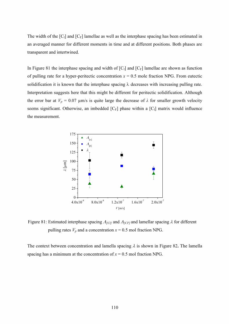
110
The width of the [Cl] and [CF] lamellae as well as the interphase spacing has been estimated in
an averaged manner for different moments in time and at different positions. Both phases are
transparent and intertwined.
In Figure 81 the interphase spacing and width of [Cl] and [CF] lamellae are shown as function
of pulling rate for a hyper-peritectic concentration x = 0.5 mole fraction NPG. From eutectic
solidification it is known that the interphase spacing decreases with increasing pulling rate.
Interpretation suggests here that this might be different for peritectic solidification. Although
the error bar at Vp = 0.07 µm/s is quite large the decrease of λ for smaller growth velocity
seems significant. Otherwise, an imbedded [CF] phase within a [Cl] matrix would influence
the measurement.
4.0x10⁻⁸
8.0x10⁻⁸
1.2x10⁻⁷
1.6x10⁻⁷
2.0x10⁻⁷
0
25
50
75
100
125
150
175
[
m]
V [m/s]
[]
[]
Figure 81: Estimated interphase spacing [Cl] and [CF] and lamellar spacing for different
pulling rates Vp and a concentration x = 0.5 mol fraction NPG.
The context between concentration and lamella spacing is shown in Figure 82. The lamella
spacing has a minimum at the concentration of x = 0.5 mol fraction NPG.

111
0.46 0.48 0.50 0.52 0.540
30
60
90
120
150
180
210
240
[CF]
[Cl]
[
µm
]
x
Figure 82: The interphase spacing and width of [Cl] and [CF] lamellae are shown as function
of concentration for Vp = 0.19 µm/s.
Finally, it is worth mentioning that the ratio of lamella width to interphase spacing is in good
agreement with the position of x within the peritectic interval.
6.2.6 Microstructure Selection within the Peritectic Interval
Hunziker et al. [37] published equations to calculate the microstructure map of the metallic
peritectic systems Ni – Cu under the assumption that constitutional undercooling ahead of the
solid/liquid interface exists and with diffusion in the liquid [2]. Based on the experiments the
calculated microstructure map and the experimental results for the peritectic region of the
binary organic phase diagram NPG - TRIS are shown in Figure 83. The microstructure map is
calculated with the measured diffusion coefficient and the difference between the calculated
solidus and the liquidus temperature (see chapter 4.1). It has to be mentioned that
solidification morphologies at a higher GT/Vp ratio of 1.7·10-11
s·K/m² need more than 4 hours
to reach steady state conditions. The calculations predict the appearance of mixed bands for
concentrations between x = 0.475 and 0.505 mol fraction NPG.

112
0.44 0.46 0.48 0.50 0.52 0.54 0.56
404
406
408
410
412
414
416
TP
C[L]
C[CF]
NPGTRIS
[CF][C
l+C
F][C
l]
[L+CF]
[L]
[L+Cl]
C[Cl]
hypo-peritectic hyper-peritectic
Tem
per
atu
re [
K]
x
0.44 0.46 0.48 0.50 0.52 0.54 0.56
0.0
5.0x10¹⁰
1.0x10¹¹
1.5x10¹¹
2.0x10¹¹
2.5x10¹¹
GT /
Vp [
K s
/m2]
x
planar front
cells
dendrites
bands
PCG
oscillation
Figure 83: Peritectic region of the phase diagram and calculated microstructures depending
on the applied GT/Vp and the mol fraction NPG x as full lines. The region where
layered structure formation is possible is shaded in grey. The dots show the
experimental solidification morphology for dendrites, cells and planar front after
having reached theoretically stable growth conditions. Metastable solidification
morphologies are shown in the graph even before the reach of steady state growth
conditions. Note that the experimental points below the dotted line represent
experiments taken at less than 4 hours.
113
For all concentrations below that region the change from planar to dendritic growth is
predicted for a nearly constant ratio GT/Vp 1.2·1011
s·K/m², for concentrations above that
region the change is situated at about GT/Vp 4·1010
s·K/m². The experimental GT/Vp
microstructure map has been established with several different concentrations and pulling
rates. Figure 83 shows the measured GT/Vp - x microstructure map with the estimated
diffusion coefficient from chapter A.9.
Since the TRIS rich [Cl] plastic phase is stable for only 4 hours at the selected process
conditions, the solidification morphology at the calculated steady-state time was selected if
smaller than 4 hours. These investigations reproduce the predicted step in the GT/Vp
microstructure map between the [Cl] and [CF] phase as a consequence of the different T0 at
the same concentration [40] in the far hypo- and hyper-peritectic region. It shows the
oscillating solidification morphology along the region where the cellular solidification
changes to a planar front. Furthermore, the region where coupled growth occurs is within the
peritectic region. Both solidification morphologies have in common an initial unstable banded
structure.

114
7 Conclusions and Future Needs
In the present work, solidification morphologies in the hypo- and hyper-peritectic region were
studied. The investigations were done at solidification rates close to the limit of constitutional
undercooling in a binary organic system which shows a peritectic reaction. The work includes
additional investigations such as estimation of viscosity, heat coefficient, vapor pressure and
DSC measurements to identify necessary physical and chemical properties. The results of the
experiments show the following insights:
Annealing experiments indicate a thermal instability for pure TRIS and its alloys if the
material is kept at a temperature above the solid/solid transition at 406 K.
DSC measurements show a thermal stability for pure TRIS and its alloys if the
material is kept at a temperature of 453 K no longer than 4 hours.
The reported phase diagram by Barrio et al. [50] has been confirmed by DSC
measurements within the expected measurements errors in a fixed temperature
gradient. Also good agreement was achieved by studying the corresponding
solid/liquid interface positions of various alloys.
The main investigation focuses on controlled solidification at selected concentrations within a
micro Bridgman-furnace. Rectangular glass samples were filled with an alloy and pulled
through the furnace. In-situ solidification morphology was observed with a microscope in
combination with a CCD camera. The solidification morphologies were recorded and stored
for further investigation. The following can be stated:
The determined melting points of the selected concentrations were be confirmed by in-
situ observations.
When holding a sample with a TRIS - NPG alloy stationary within a constant
temperature gradient the plastic phase is stable for 4 hours. Afterwards, the TRIS-rich
phase [Cl] gradually disappears and the facetted phase [O] contacts with the liquid
phase after 18 hours. The NPG-rich [CF] phase appears to be more stable.
After full dissolution, the plastic phase can be re-established by cooling the entire
sample and re-starting the experiment. In this case, the decomposition is faster.

115
Under pulling conditions the thermal instability of TRIS lowers permanently the
melting temperature due to the long expose time at high temperature during the
experiments.
The effective diffusion coefficient Deff is estimated for the entire phase diagram
although the plastic phase disappears. This is done by the determination of the
migration of droplets through the matrix phase. The measured diffusion coefficient DL
is in the average order of 2.1·10-11
0.6 m2/s for concentrations 0.47 x 0.54 mol
fraction NPG.
Bands, oscillating growth, and coupled growth solidification morphologies were found
in the hypo-peritectic region. The results are partly reproducible. In the most cases
partial layered structure formation were observed which is predicted under the
presents of convection. The position agrees with theoretical predictions for
solidification morphologies in the presence of convection.
Investigation in the hypo-peritectic composition regions shows an oscillatory behavior
of the dendritic/planar liquid-solid interface for a constant pulling velocity. This
behavior is not predicted for the formation of layered structures and it is for the first
time observed in-situ.
Both plastic phases which participate at a peritectic growth, namely [Cl] and [CF], are
optically undistinguishable. To distinguish between the plastic phases [Cl] and [CF],
concentrations in the TRIS-rich and in the NPG-rich regions are investigated under the
same process conditions. In order to indicate which growth mode occurs for a given
concentration C0, temperature gradient GT, pulling velocity, Vp and the corresponding
morphology is mapped as a function of alloy composition and GT/Vp ratio.
Up to now no evidence has been found for peritectic reaction during coupled growth
solidification.
The intended experiments on ISS to determine the effect of the natural convection on
the solidification morphologies wasn’t investigated. This will not be done before 2014.
The collected information improves the understanding of peritectic solidification, however,
the results are influenced by decomposition and convection. Further investigations are
required without convection. For that, experiments in space are highly desired. Additionally
investigations of further organic phase diagrams which also show a peritectic reaction are
proposed to increase the understanding of the observed solidification morphologies.
116
8 Summary
In the last century investigations on peritectic metallic systems show a wide range of possible
microstructures. Bands, islands, tree-like microstructures and coupled growth were detected at
growth rates where both phases can solidify with a planar front. The investigations were done
by experiments and numerical simulations. Whereby, all these microstructures are highly
influenced by convection and undercooling in front of the solid/liquid interface.
In the present study, the organic compound TRIS - NPG was used as a model substance for
in-situ observation of peritectic solidification. It is the first time that peritectic solidification is
directly observed at velocities close to the limit of constitutional undercooling. Both organic
compounds have high temperature non-faceted phases which solidify in the same manner as
metals do. Non-faceted phases, called plastic phase, occur with almost the same transparent
color. Therefore, they are optically undistinguishable and only the solid/solid interface
between the transparent plastic phases [Cl] and [CF] and the solid/solid interface with the
facetted phase [O] is visible. Due to the high temperature of the Bridgman-furnace and the
long observation time the plastic phase [CF] of TRIS can be used only limited within a tight
experimental border conditions.
For hypo-peritectic concentrations the growth of bands with thickness from 76 µm to 190 µm
were observed. The observed banded solidification was not stable and led to coupled growth.
Evidence for this form of transformation were found previously in experiments with metals
and supported with numerical simulation. The transformation from a banded structure to
coupled growth is discussed in literature. Here, it was the first time that the transformation
from banded to coupled growth could be directly observed. Unexpected, unstable oscillating
behavior was found where both phases grow in a competitive manner at the same time. This
observed solidification pattern occurs for process conditions where layered structures are not
discussed in literature. Beside the oscillatory growth mode, direct isothermal coupled
peritectic growth was observed. This eutectic-like solidification pattern is stable and shows a
typical spacing of = 142 to 201 µm. Investigations near the peritectic concentration, where
mixed bands are predicted, require finer adjustment in the variation of the alloy composition.
However, this is postponed to further research work.

117
9 References
[1] European Space Agency Contract DRD-E18, “DIRSOL Preliminary Design Report”, (2008) 235.
[2] W.Kurz, D.J.Fischer, “Fundamentals of solidification”, Trans tech Publications Ltd 1998 [ISBN 0-87849-
804-4].
[3] S.T. Misture, D.P. Matheis, R.L. Snyder, T.N. Blanton, G. M. Zorn, B. Seebacher,
Physica C: Superconductivity, 250 (1995) 175-183.
[4] D.R. Uhlmann and G.A. Chadwick, Acta Metall. 9 (1961) 835–840.
[5] W.J.Boettinger, Metall.Trans. 5 (1974) 2023 - 2031.
[6] R.Trivedi and J.S.Park, J. Cryst. Growth 235 (2002) 572 - 588.
[7] R. Trivedi and J.H. Shin, Mater. Sci. Eng. A 413–414 (2005) 288–295.
[8] H.Yasuda, N.Notake, K.Tokieda and I.Ohnaka, J. Cryst. Growth 210 (2000) 637–645.
[9] F.Kohler, L.Germond, J.D. Wagniére and M.Rappaz, Acta mater 57 (2009) 56-68.
[10] A.Karma, W.J.Rappel, B.C.Fuh and R.Trivedi, Metall. Trans. 29A (1998) 1457–1470.
[11] K.Tokieda, H.Yasuda and I.Ohnaka, Mater. Sci. Eng. A262 (1999) 238–245.
[12] T.A.Lograsso, B.C.Fuh and R.Trivedi, Metall. Trans. 36A (2005) 1287–1300.
[13] S.Liu and R.Trivedi, Metall. Trans. 37A (2006) 3293–3304.
[14] X.W.Hu, S.M.Li, W.J.Chen, S.F.Gao, L.Liu. and H.Z.Fu, J. Alloys and Compounds 484 (2009) 631-636.
[15] D.Ma, Y.Li, S.C.Ng and H.Jones, Acta Mater. 48 (2000) 1741–1751.
[16] D.Ma, Y.Li, S.C.Ng and H.Jones, Acta Mater. 48 (2000) 419–431.
[17] Y.Li, S.C.Ng and H.Jones, Scripta Mater. 39 (1998)7–11.
[18] X.W.Hu, S.M.Li, L.Liu and H.Z.Fu, China Foundry 5 (2008) 167–171.
[19] A.P.Titchener and J.A.Spittle, Acta Metall. 23 (1975) 497–502.
[20] Y.Q.Su, C.Liu, X.Z.Li, J.J.Guo, B.S.Li, J.Jia and H.Z.Fu, Intermetallics 13 (2005) 267–274.
[21] P.Busse and F.Meissen, Scripta Mater. 36 (1997) 653–658.
[22] L.S.Luo, Y.Q.Su, J.J.Guo, X.Z.Li, S.M.Li, H.Zhong, L.Liu and H.Z.Fu, J. Alloys Compd. 461 (2008)
121–127.
[23] Y.Q.Su, L.S.Luo, X.Z.Li, J.J.Guo, H.M.Yang and H.Z.Fu, Appl. Phys. Lett. 89 (2006)
2319181-2319183.
[24] L.S.Luo, Y.Q.Su, X.Z.Li, J.J.Guo, H.M.Yang and H.Z.Fu, Appl. Phys. Lett. 92, (2008)
0619031-0619033.
[25] M.Vandyoussefi, H.W.Kerr and W.Kurz, Acta Mater. 48 (2000) 2297–2306.
[26] T.S.Lo, S.Dobler, M.Plapp, A.Karma, and W.Kurz, Acta Mater. 51 (2003) 599-611.
[27] S. Dobler, T.S.Lo, M.Plapp, A.Karma and W.Kurz, Acta Mater. 52 (2004) 2795-2808.
[28] Massaki Sumida, Journal of Alloys and Compounds 349 (2003) 302-310.
[29] Z.Feng, J.Shen, Z.Min, L.Wang and H.Fu, Materials Letters 64 (2010) 1813-1815.
[30] M.Vandyoussefi, H.W.Kerr and W.Kurz, Acta Mater. 45 (1997) 4093-4105.
[31] L.S.Luo, Y.Q.Su, J.J.Guo, X.Z.Li and H.Z.Fu, Sci China-Phys mech. Astron 50 (2007) 442-450.
[32] J.H.Lee and J.D.Verhoeven, J. Cryst. Growth 144 (1994) 353–366.
[33] Q.L.Rao, X.L.Fan, D.Shu and C.C.Wu, J. Alloys Compd. 461 (2008) L29–L33.
[34] H.Zhong, S.M.Li, H.Y.Lü, L.Liu, G.R.Zou and H.Z.Fu, J. Cryst. Growth 310 (2008) 3366–3371.
[35] H.W.Kerr and W.Kurz, Int. Mater. Rev. 41 (1996) 129–164.
[36] W.Luo, J.Shen, Z.Min and H.Fu, J. Cryst. Growth 24 (2008) 5441–5446.
[37] O.Hunziker, M.Vandyoussefi and W.Kurz, ActaMater 46 (1998) 6325–6336.
[38] W.Z. Luo, J. Shen, Z.X. Min and H.Z. Fu, Mater. Lett. 63 (2009)1419–1421.
[39] T.A. Lagrasso, B.C. Fuh and R. Trivedi, Met. Mat. Trans. A 36A (2005) 1287 – 1300.
[40] O.Hunzinger, M.Vandyoussefi and W.Kurz, Acta mater 46 (1998). 6325-6336.
[41] R. Trivedi, Metall. Mater. Trans. 26A (1995) 1583-1590.
[42] P.Mazumder, R.Trivedi and A.Karmer, Met. Mat. Trans. 31A (2000) 1234-1246.
[43] R.Trivedi, Scripta Mat.53 (2005) 47-52.
[44] R.Rudman, Solid State Commun. 29 (1979) 785-787.
[45] J.Timmermans, J.Phys.Chem.Solids. 18 (1961) 1 - 8.
[46] L.A.K.Staveley, Annu. Rev. Phys. Chem. 13 (1962) 351 - 368.
[47] P.R.Sahm, I.Egry, T. Volkmann, “Schmelze, Erstarrung, Grenzflächen”, Vieweg Verlag [ISBN 3-528-
06979-1].
[48] W.J. Dunning, J.Phys.Chem.Solids. 18 (1961) 21.
[49] http:// www.merck.de
[50] M.Barrio, D.O.Lopez, J.L.Tamarit, P.Negrier and Y.Haget, J. Mater. Chem. 5 (1995) 431 - 439.
[51] D.Eilerman and R.Rudman, J.Chem.Phys.72 (1980) 5656-5666.
[52] L.Sturz, V.T.Witusiewicz, U.Hecht and S.Rex, J. Crystal Growth 270 (2004) 273 - 282.

118
[53] V.T.Witusiewicz, L.Sturz., U.Hecht and S. Rex, Acta Mater. 53 (2005) 173 - 183.
[54] S.Akamatsu and G.Faivre, Phys. Rev. E 58 (1998) 3302. – 3314.
[55] S.Akamatsu, M.Plapp, G.Faivre and A.Karma, Phys. Rev. E 66 (2002) 0305011 - 0305014.
[56] V.T.Witusiewicz, L.Sturz, U.Hecht and S.Rex, Acta Mater. 52 (2004) 5071 - 5081.
[57] M.Barrio, D.O.Lopez, J.L.Tamarit, P. Negrier and Y .Haget, J. Solid State Chem. 124 (1996) 29-38.
[58] D.O.Lopez, J.Van Braak, J.L.Tamarit and H.A.J.Oonk, Calphad 19 (1995) 37 - 47.
[59] D.Chandra and R.Chellappa, W.M.Chien, J. Phys.Chem. Solids 66 (2005) 235 – 240.
[60] http://www.chem.unep.ch
[61] J.P.Mogeritsch, A.Ludwig, S.Eck, M.Grasser and B.J.McKay, Scripta Mat. 60 (2009) 882-885.
[62] http://en.wikipedia.org/wiki/Tris
[63] J.Ll.Tamarit, Mol. Cryst. Liq. Cryst. 250 (1994) 347-358.
[64] R.E.Wasylishen, P.F.Barron and D.M.Doddrell, Aust. J. Chem. 32 (1979) 905 -909.
[65] http://www.dow.com/
[66] S.M.Rowe, Org. Proc. Research & Dvelop. 6 (2002) 877-883.
[67] http://www.vitrocom.com.
[68] G.W.H.Höhne, W.Hemminger, H.-J.Flammerheim, “Differential Scanning Calorimetry”, Springer-Verlag
Berlin [ISBN 3-540-59012-9].
[69] W.J.Boettinger, U.R.Kattner, K.-W.Moon, J.H. perepezko, “DTA and Heat-flux DSC Measurements of
Alloy Melting and Freezing“, National Institute of Standards and Technology [Spec.Publ. 960-15].
[70] http://www.faulhaber.com/
[71] http://www.eurotherm.com
[72] Prof. Paul O´Leary, Institute for Automation, University of Leoben, Peter-Tunnerstraße 27, Leoben
[73] Y.Ocak, S.Akbulut,K.Keslioglu and N.Marasli, J. Colloid and Interface Science 320 (2008) 555-562.
[74] V.T.Witusiewicz, L.Sturz, U.Hecht and S.Rex, Acta Mater. 52 (2004) 5519 - 5527.
[75] A.Ludwig, J.Mogeritsch and M.Grasser, Trans. Ind. Inst. Metals 62 (2009) 433-36.
[76] J.P.Mogeritsch, S.Eck, M.Grasser and A.Ludwig, Mater. Sci. Forum 649 (2010) 159-64.
[77] http://lb.chemie.uni-hamburg.de
[78] http://www.sigmaaldrich.com
[79] N.N.Brandt, A.Y.Chikishev and I.K.Sakodinskaya, J.Molc. Str. 648 (2003) 177-182.
[80] B.Granzow, P. Klaeboe and V. Sablinskas, J.Molc. Str. 349 (1995) 153-156.
[81] Z.Zhang and Y.Xu, Solar Energy 71 (2001) 299-303.
[82] Z.Zhang, Y.Xu and M.Yang, J. Chem. Data 45 (2000) 1060-1063.
[83] S.Akbulut, Y.Ocak, K.Keslioglu and N. Marasli, J. Phy. Chem. Solid 70 (2009) 72-78.
[84] S.Divi, R.Chellapa and D.Chandra, J.Chem. Thermodynamics 38 (2006) 1312-1326,
[85] D.Chandra, W.Chien, V.Gandikotta and D.W. Lindle, Z. Phys. Chem. 216 (2002) 1433-1444.
[86] Z.Z.Ying and Y.M.Lin, J. Chem. Thermodynamics 22 (1990) 617-622.
[87] http://www.weblo.com/domain/available/bestvibes.com
[88] http://www.astm.org/DATABASE.CART/HISTORICAL/D5930-97.htm
[89] http://www.carlroth.ch/catalogue
[90] http://www.kayelaby.npl.co.uk/chemistry
[91] G.M.Barrow,”Physical Chemistry”, McGraw-Hill Inc., 1973 [ISBN 3-528-23806-2].
[92] http://www.cheric.org/kdb/kdb/hcprop/showcoef.php?cmpid=922&prop=PVP
[93] http://chem.sis.nlm.nih.gov/chemidplus/
[94] www.perstorp.com/layouts/ViewFile.aspx?prodid=66&langid=1&filetype=msds –
[95] J.Font and J.Muntasell, Mat. Research Bulletin. 30 (1995) 479-489.
[96] http://web.grcc.edu/Pr/msds/Biology/Tris%20Base%20-%20Genomic%20Solutions.pdf
[97] http://www.koeichem.com/english/index.htm
[98] http://www.brookfieldengineering.com/products/viscometers/laboratory.asp
[99] http://en.wikipedia.org/wiki/Viscometer
[100] http://www.basf.com/group/corporate/de/index
[101] S.Liu, J.Teng and J.Choi, Metall. Mat. Trans. 38A (2007) 1555-1562.
[102] E.Hecht, A.Zajac, “Optics“, Fourth Edition. Pearson Higher Education. [ISBN 9780321188786].

119
10 Symbols
Symbol Meaning Definitions Units
C concentration C = x100 % mol.%
wt.%
C0 initial concentration mol.%
CL liquidus concentration mol.%
CS solidus concentration mol.%
Cp peritectic concentration mol.%
D diffusion coefficient m2/s
DL diffusion coefficient in the liquid m2/s
GT temperature gradient K/m
M molar mass g/mol
N Avogadro number 6.0221023
mol-1
Q heat flow W Q heat stream W/s
R gas constant 8.314 J/Kmol
Tb boiling temperature K
Tc temperature in the cold zone of the Bridgman-furnace K
Tcold extrapolated peak completions temperature of a DSC curve K
Te extrapolated peak onset temperature of a DSC curve K
Tf finish peak temperature of a DSC curve K
Thot temperature in the hot zone of the Bridgman-furnace K
Ti initial peak temperature of a DSC curve K
TL liquidus temperature K
Tm melting temperature K
Tm maximum peak temperature of a DSC curve K
Tp peritectic temperature K
TS solidus temperature K
TSST transition temperature solid/solid K
T
S solidus temperature of the [] phase K
T
S solidus temperature of the [] phase K
V growth or solidification velocity m/s
Vc critical solidification velocity m/s
VL lateral solidification velocity m/s
Vp pulling rate m2/s
Vs molar volume, m3/mol
V solidification velocity of the [phase m/s
V solidification velocity of the [phase m/s
X length of the adiabatic gap m
atoms per cell -
[CF] face center cubic, non-faceted phase , optical inactive phase
or high temperature phase of NPG and NPG rich alloys -
[Cl] body center cubic, non-faceted phase , optical inactive phase
or high temperature phase of TRIS and TRIS rich alloys -
[M] monocline, faceted phase , optical active phase or low
temperature phase of NPG -
[O] orthorhombic, faceted phase , optical active phase or low
temperature phase of TRIS -
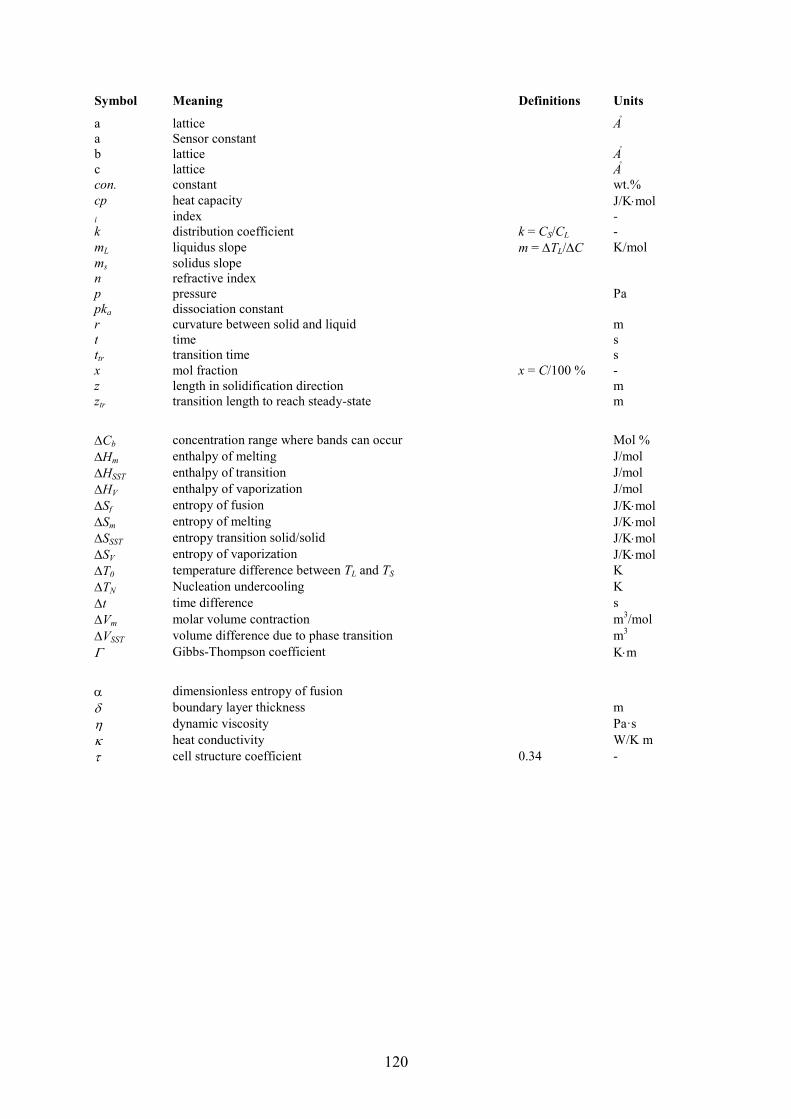
120
Symbol Meaning Definitions Units
a lattice Ả
a Sensor constant
b lattice Ả
c lattice Ả
con. constant wt.%
cp heat capacity J/Kmol
i index -
k distribution coefficient k = CS/CL -
mL liquidus slope m = TL/C K/mol
ms solidus slope
n refractive index
p pressure Pa
pka dissociation constant
r curvature between solid and liquid m
t time s
ttr transition time s
x mol fraction x = C/100 % -
z length in solidification direction m
ztr transition length to reach steady-state m
Cb concentration range where bands can occur Mol %
Hm enthalpy of melting J/mol
HSST enthalpy of transition J/mol
HV enthalpy of vaporization J/mol
Sf entropy of fusion J/Kmol
Sm entropy of melting J/Kmol
SSST entropy transition solid/solid J/Kmol
SV entropy of vaporization J/Kmol
T0 temperature difference between TL and TS K
TN Nucleation undercooling K
t time difference s
Vm molar volume contraction m3/mol
VSST volume difference due to phase transition m3
Gibbs-Thompson coefficient Km
dimensionless entropy of fusion
boundary layer thickness m
dynamic viscosity Pa·s
heat conductivity W/K m
cell structure coefficient 0.34 -

1
A Appendix: Determination of Material Properties
A.1 Variation of Material Purifications
Introduction
In this part of the thesis the effect of different material purifications on the organic substances
TRIS and NPG was tested. Barrio et al. [50] reported that the purity of NPG can be increased
by applying a drying process at about 310 K for several hours. NPG is very hydroscopic and
contains as delivered usually residual water. Therefore, a pretreatment of the organic
compounds seems to be necessary for further use in his studies [61].
Experimental investigations
To improve the purity of the organic substances two different methods of purification were
tested: (i) purification by drying and (ii) purification by sublimation. A DSC measurement
was performed to test the impact of the purification method on the organic substances. After
the purification process NPG and TRIS was directly used for the alloy preparation.
Purification by drying
For purification of NPG and TRIS a heater with a flat glass container filled with the organic
material was placed into the glove box (see chapter 3.1). Then the organic compound heated
up to 310 K for more than 24 hours. During that time NPG changed its appearance from a
white snow-like crystalline material to a white sugar-like powder. TRIS is a white powder and
shows no optically visible effects during the drying process.
Purification by sublimation
Figure 84 shows a sketch of the used sublimation device. It consists of a double glass bottle
with a cooling finger located in the middle axis of one part of the device. The finger is cooled
by connecting the fittings with a water supply. Due to the size of the device it is not possible
to operate the system within the glove box. Hence the sublimation has to be done outside of
the glove box whereas the filling has to be done within the glove box. 10 - 20 g of organic
compounds together with 50 vol.% molecular sieve (Aldrich Cat. No. 20.858-2) is filled into
the sublimation device. To avoid moisture absorption by the hydroscopic organic compounds
during purification a molecular sieve was used within the sublimation device. After the filling
the device is carefully removed from the glove box and put into an oil bath. Here it is heated
for several hours. During purification, the solid material sublimates and freezes again at the

2
cooling finger. The applied sublimation parameters are given in Table 12. After the
sublimation procedure the purification device is put back into the glove box.
Figure 84: The sublimation device consists of a double glass bottle with a cooling finger
located in the middle axis of one part of the device. The organic compound
together with 50 vol.% molecular sieve is filled into the device for purification.
The purified material is taken from the cooling finger and the glass device is filled again.
Approximately 0.5 g material is prepared by one single sublimation cycle.
Table 12: Sublimation parameters for purification.
Parameters
Temperature of the oil bath 353 K
Temperature of the cooling finger 283 K
Sublimation time 24 h
Results and Discussion
TRIS decomposes during the purification by sublimation, which was visible by long dark and
light brown threads at the cooling finger. Only NPG shows no optical visible effects. To
evaluate the effect of sublimation on NPG, the liquidus temperature of NPG as delivered and
the sublimated material was measured by DSC measurement. The exact procedure and
evaluation of the DSC measurement [67, 68] was done in the same way as descript in details
in chapter 4.3.2. For all samples, the difference between the liquidus temperatures before and
after purification is very small. The liquidus temperature of the purified material lies within
the accuracy of the DSC measurement (see Figure 85). All three curves show a characteristic
sharp end of the peak which is characteristic for the used material. All DSC measurements
show a smooth increase of the curve from the basic line to the peak maximum. After
water supply line
cooling finger
organic compound molecular sieve
oil bath
heater

3
purification the material seems to have a higher solidus temperature than the material as
delivered, but again, the difference between the different purified materials is within the
measurement accuracy. All in all, the difference between the liquidus and solidus
temperatures of purification by sublimation and drying is very small and lies within the
accuracy of the DSC measurement.
399 400 401 402 403 404 405 4066
8
10
12
14
16
18
Hea
t fl
ow
[m
W]
Temperature [K]
Tl = 402.1 ± 0.7 K, T
s = 398.1 ± 1 K (NPG as delivered)
Tl = 402.3 ± 0.5 K, T
s = 399.7 ± 1 K (NPG after drying)
Tl = 402.5 ± 0.4 K, T
s = 400.1 ± 1 K (NPG after sublimation)
Figure 85: DSC curves for NPG as delivered and for two purified materials. It is obvious
that by the drying process a substantial purification can be achieved, visible in
the change of the solidus temperature.
Furthermore, the alloy preparation includes an additionally purification method (see
chapter 3.1.1), where impurities with lower boiling points are removed by sublimation. For
this reason, NPG and TRIS were only purified by long time drying before it was directly used
for the alloy preparation.
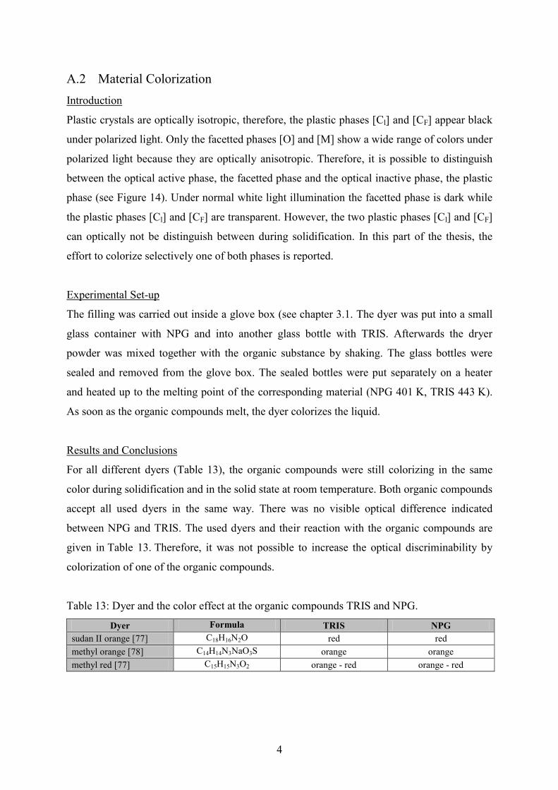
4
A.2 Material Colorization
Introduction
Plastic crystals are optically isotropic, therefore, the plastic phases [Cl] and [CF] appear black
under polarized light. Only the facetted phases [O] and [M] show a wide range of colors under
polarized light because they are optically anisotropic. Therefore, it is possible to distinguish
between the optical active phase, the facetted phase and the optical inactive phase, the plastic
phase (see Figure 14). Under normal white light illumination the facetted phase is dark while
the plastic phases [Cl] and [CF] are transparent. However, the two plastic phases [Cl] and [CF]
can optically not be distinguish between during solidification. In this part of the thesis, the
effort to colorize selectively one of both phases is reported.
Experimental Set-up
The filling was carried out inside a glove box (see chapter 3.1. The dyer was put into a small
glass container with NPG and into another glass bottle with TRIS. Afterwards the dryer
powder was mixed together with the organic substance by shaking. The glass bottles were
sealed and removed from the glove box. The sealed bottles were put separately on a heater
and heated up to the melting point of the corresponding material (NPG 401 K, TRIS 443 K).
As soon as the organic compounds melt, the dyer colorizes the liquid.
Results and Conclusions
For all different dyers (Table 13), the organic compounds were still colorizing in the same
color during solidification and in the solid state at room temperature. Both organic compounds
accept all used dyers in the same way. There was no visible optical difference indicated
between NPG and TRIS. The used dyers and their reaction with the organic compounds are
given in Table 13. Therefore, it was not possible to increase the optical discriminability by
colorization of one of the organic compounds.
Table 13: Dyer and the color effect at the organic compounds TRIS and NPG.
Dyer Formula TRIS NPG
sudan II orange [77] C18H16N2O red red
methyl orange [78] C14H14N3NaO3S orange orange
methyl red [77] C15H15N3O2 orange - red orange - red

5
A.3 Boiling Point
Introduction
The boiling temperature Tb of pure NPG is given for p = 760 mm Hg (standard pressure) [49]
and of pure TRIS for p = 10 mm Hg [49]. The boiling point of pure TRIS cannot be found in
the literature at standard pressure. Therefore, the boiling temperature at standard pressure for
pure TRIS and selected concentrations were determined (Table 12).
Experimental Set-up
The samples are filled inside a glove box (argon atmosphere) whereas the further
experimental proceeding was done under normal atmosphere. The organic compounds with
the required concentration are first put into a glass container. The glass container opening was
closed with a metal cap which revealed a small hole for a thermal element. This hole was
sealed with silicon and a scotch tap till it was used. The glass container was put on a hot plate
of a heater, the scotch tape was removed and a thermo sensor was drilled through the sealed
hole. The height of the container, the form of the metal cap and the sealing material silicon
enables to neglect a possible increase in pressure inside the glass container. The position of
the thermo sensor was chosen next to the bottom of the container. As soon as the liquid
material starts to boil the temperature had been recorded. This process was carried out for the
two pure compounds and alloy concentrations in steps of 10 %.
Results and Conclusions
The determination of the boiling point of TRIS gives a temperature at 553 ± 2 K. At the
boiling point the material changes the color from transparent to light brown. The same
happens to alloys with a high concentration of TRIS, like x = 0.1 or 0.2 mol fraction NPG (see
Figure 86). All other materials stay transparent during boiling. The obtained values are given
in Table 14 and shown in Figure 86. The obtained boiling temperature does not follow a linear
relationship with the alloy concentration. The boiling temperatures increase nearly linearly
from pure NPG to a concentration of 0.20 mol fraction NPG and then increase further till pure
TRIS is reached (see Figure 86). TRIS decomposes which is visible in a change of the color of
the liquid material in the glass samples from transparent to brown. The same happens do
alloys with x = 0.10 and 0.20 mol fraction NPG. All other alloys stay transparent in the liquid
phase and become white after cooling from the boiling temperature (see the pictures of the
samples after the experiment in Figure 86 at room temperature).
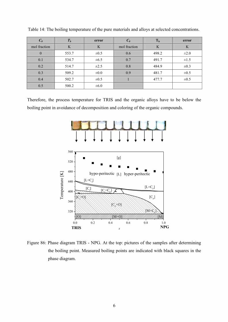
6
Table 14: The boiling temperature of the pure materials and alloys at selected concentrations.
C0 Tb error C0 Tb error
mol fraction K K mol fraction K K
0 553.7 ±0.5 0.6 498.2 ±2.0
0.1 534.7 ±6.5 0.7 491.7 ±1.5
0.2 514.7 ±2.5 0.8 484.9 ±0.3
0.3 509.2 ±0.0 0.9 481.7 ±0.5
0.4 502.7 ±0.5 1 477.7 ±0.5
0.5 500.2 ±6.0
Therefore, the process temperature for TRIS and the organic alloys have to be below the
boiling point in avoidance of decomposition and coloring of the organic compounds.
0.0 0.2 0.4 0.6 0.8 1.0
320
360
400
440
480
520
560
[g]
Tem
per
ature
[K
]
x
[L]hypo-peritectic hyper-peritectic
[L+Cl]
[L+CF]
[Cl+C
F]
[Cl]
[Cl+O]
[CF+O]
[CF]
[M+CF]
[M+O][O] [M]
TRIS NPG
Figure 86: Phase diagram TRIS - NPG. At the top: pictures of the samples after determining
the boiling point. Measured boiling points are indicated with black squares in the
phase diagram.

7
A.4 Raman Spectroscopy
Introduction
TRIS and alloys with higher TRIS concentration, x ≥ 0.2 mol fraction NPG, show a change of
the color after being melted and solidified, see chapter A.3. This behavior indicates a probable
decomposition of TRIS [64] in the liquid state of TRIS. A decomposition of pure TRIS could
be caused by a decrease of the covalent bonds within the molecules. Each bond oscillates with
a certain energy which can be measured with Raman spectroscopy. Such a spectrum is an
exclusive fingerprint for each material. If an organic material changes its bonds during
heating-up, the Raman spectrum changes. Therefore, TRIS as delivered and an alloy with
x = 0.3 mol fraction NPG was investigated with Raman spectroscopy before and after
solidification investigations in the Bridgman-furnace. The Raman spectra of TRIS can be
found in N.N. Brandt et al. [79] whereas B. Granzow [80] published the Raman spectra of the
solid and the plastic phase of NPG.
Experimental Set-up
For the investigation a Dilor LABRAM confocal-Raman spectrometer was used (see Figure
87). TRIS as delivered, unused prepared alloys and used alloys (from the boiling point
experiments) were used for the Raman spectroscopy.
Figure 87:
Dilor LABRAM equipped with a
frequency-doubled Nd-YAG laser
(100 mW, 532.2 nm) and with a He-
Ne laser (633 nm) and diffraction
gratings of 1200 and 1800
grooves/mm.
The detection is performed with a Peltier-cooled, slow-scan, CCD matrix-detector. Laser
focusing and sample viewing are performed through an Olympus BX 40 microscope fitted
with 10X, 50X and 100X long-working distance objective lenses (allowing viewing in
reflected- and transmitted-light). Samples can be held at controlled temperatures
between 83 K and 873 K using a Linkam THMSG 600 heating-freezing stage. Sample images
are acquired by a color video-camera and projected on a video monitor. Both, the Raman

8
spectra and the sample images, are processed on a 333 MHz Pentium computer.
Results
The Raman spectra of pure TRIS as delivered and after cooling from the liquid phase to room
temperature are given in Figure 88. TRIS as delivered shows a clear spectrum but the same
material after heating-up and cooling down shows a shift of the curve to a general higher level
indicated by the red line in Figure 88.
600 800 1000 1200 1400 16000
10000
20000
30000
40000
50000
60000
Ram
an i
nte
nsi
ty [
arbit
rary
unit
s]
unheated phase, white color
heated phase, brown color
wave number [1/cm]
Figure 88: Raman Spectra for pure TRIS as delivered (black line) and after cooling down
from the liquid phase (red line). The red line shows a higher intensity level with
smaller peaks.
Figure 89 shows the Raman spectra for the alloy with x = 0.3 mol fraction NPG before and
after solidification investigation. It is observable that the alloy and the reheated alloy show a
higher energy level than the pure organic substances TRIS and NPG. Each peak shows the
vibration energy in general, and both curves show the same tenor of peaks, but differ in detail
of the Raman intensity.

9
200 400 600 800 1000 1200 1400 16002000
4000
6000
8000
10000
12000
14000
16000
18000
20000
Ram
an i
nte
nsi
ty [
abb
itra
ry u
nit
s]
unheated phase, white color
heated phase, brown color
wave number [1/cm]
Figure 89: Raman spectrum of an unused alloy x = 0.3 mol fraction NPG and an alloy after
being liquid and became brown colored.
Conclusions
The peaks of the used material are at the same position as the peaks of TRIS as delivered
which indicates that the atomic bounding are still intact. After heating-up, TRIS shows a
florescence, this can be seen by a shift of the curve to a higher level. During the investigation
the material absorbs the energy of the laser and emits it at a higher level. Since the Raman
spectroscopy curve differs for TRIS as delivered and molten/frozen TRIS, it is clear that the
material changes its properties after heating and cooling.

10
A.5 Heat Conductivity
Introduction
The heat conductivity is one of the fundamental properties of a material. The heat
conductivity of a pure material changes with temperature but the heat conductivity of alloys
changes with temperature and concentration. Zang et al. [81] investigated the heat
conductivity of TRIS as a potential material for thermal storage of energy. In addition, Zhang
et al. [82] and Akbulut et al. [83] investigated the heat conductivity of NPG. Furthermore the
heat capacity of TRIS and NPG was investigated by Divi et al. [84], Chandra et al. [85], and
Ying et al. [86]. Based on this data, the published heat conductivity of the plastic phase lies
between 2 to 3 kJ/molK for both organic compounds. In this study, it was decided to
investigate the heat conductivity of the two pure compounds TRIS and NPG for a comparison
with the published values. Additionally, the heat conductivity of an alloy with peritectic
concentration was measured.
Experimental Set-up
The measurement of the heat conductivity was performed with the heat conductivity
measuring device type K-system II from the company Advanced CAE Technology Inc.
Ithaca, N.Y. USA [87], according to ASTM D5930-97 standard [88]. The measurements were
carried out within a temperature range of 373 K and 443 K under normal ambient pressure.
The measuring system was based on the concept of a constant infinite linear heat source in the
medial axis of a cylindrical sample chamber. Figure 90 shows the bread board construction
which was used to estimate the heat conductivity of the organic compounds and its alloy. The
measurement was carried out for pure TRIS, pure NPG, and one alloy in the peritectic region
with a concentration of x = 0.5 mol fraction NPG (Figure 16 on page 24). For each
temperature, three consecutive measurements were performed and an average value for the
heat conductivity was calculated. The sample cylinder was filled within the glove box but the
experiment itself took place outside of the glove box.

11
Figure 90: Bread board construction of the K system II to measure the heat conductivity
depending on the temperature. For a definite time t the sample material is
exposed to a definite heat stream Q . The sample cylinder is kept during this
time at a constant temperature.
Results
The heat conductivity is calculated [88] in a predominated time interval (t2 – t1) with a linear
measurement curve:
1
2ln4
.
t
t
T
Qcon
. (Eq. 19)
Here, is the heat conductivity, con. a sensor constant, Q the heat stream, and ti the
measuring time. After a measurement time of approximately 30 s the sample is cooled down
to the next favored temperature and as soon as a stable temperature is reached the next
measurement is started. Figure 91 shows the plot of temperature T versus time t.
thermocouple
measuring probe
heater bands
cylindrical sample
chamber
sample material
heat insulation
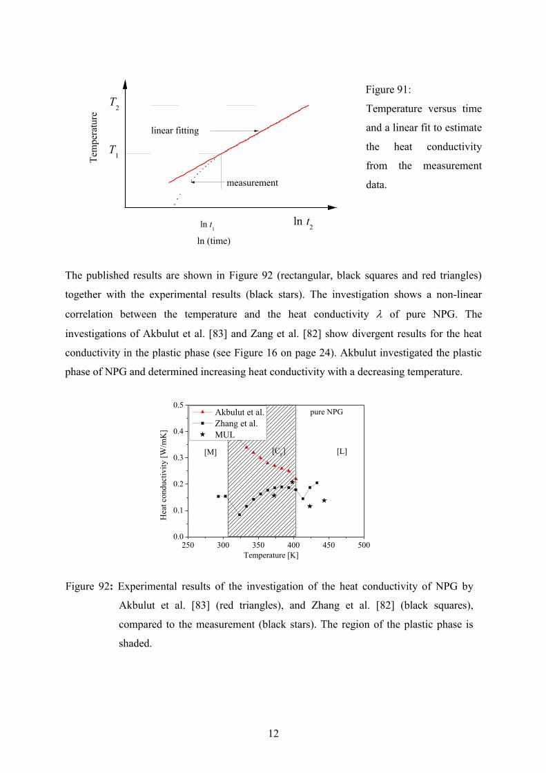
12
ln t1
ln t2
T1
Tem
per
atu
re
ln (time)
T2
linear fitting
measurement
Figure 91:
Temperature versus time
and a linear fit to estimate
the heat conductivity
from the measurement
data.
The published results are shown in Figure 92 (rectangular, black squares and red triangles)
together with the experimental results (black stars). The investigation shows a non-linear
correlation between the temperature and the heat conductivity of pure NPG. The
investigations of Akbulut et al. [83] and Zang et al. [82] show divergent results for the heat
conductivity in the plastic phase (see Figure 16 on page 24). Akbulut investigated the plastic
phase of NPG and determined increasing heat conductivity with a decreasing temperature.
250 300 350 400 450 5000.0
0.1
0.2
0.3
0.4
0.5
Temperature [K]
Hea
t co
nduct
ivit
y [
W/m
K]
Akbulut et al.
Zhang et al.
MUL
[L][CF][M]
pure NPG
Figure 92: Experimental results of the investigation of the heat conductivity of NPG by
Akbulut et al. [83] (red triangles), and Zhang et al. [82] (black squares),
compared to the measurement (black stars). The region of the plastic phase is
shaded.

13
However, the investigation done by [82] shows a decrease in heat conductivity in the plastic
phase shortly after the transition from the faceted phase to the plastic phase. The heat
conductivity is increasing in the plastic phase with increasing temperature. At the melting
point decreases and increases again in the liquid phase. The obtained experimental results of
this performed study are close to the available values of Zhang but don’t match it.
The experimentally obtained values of the heat conductivity and the published ones of pure
TRIS are shown in Figure 93.
250 300 350 400 450 5000.0
0.1
0.2
0.3
0.4
0.5
pure TRIS
Hea
t co
nduct
ivit
y [W
/m K
]
Temperature [K]
Zhang et al.
MUL
[O] [Cl] [L]
Figure 93: The graph shows the experimentally obtained values for the heat conductivity of
TRIS observed in this study (stars) compared to the results (squares) published in
[81].
In this figure the heat conductivity in the plastic phase is lower than the one observed in the
facetted or liquid phase. The heat conductivity observed in this study shows strong differences
to the published one. Only in the [Cl] region, there is an agreement with the published values.
Indeed, our measurements are in the liquid- and facetted phases are clearly below the
published values.
The investigations of the heat capacity of the alloy (x = 0.5) are shown in Figure 94. The
graph shows the heat conductivity declining with increasing temperature. The temperature
region of the plastic phase is very small at this concentration and only one measured value is
available in this region. Therefore, no essential statement can be given for the plastic phase.

14
250 300 350 400 450 5000.0
0.1
0.2
0.3
0.4
0.5
x = 0.5
Hea
t co
nduct
ivit
y [W
/m K
]
Temperature [K]
MUL
facetted phases [O+CF]
liquid phase
plastic phases
[Cl +C
F]
Figure 94: Heat conductivity of an alloy with x = 0.5 mol fraction NPG versus temperature.
The results of the heat conductivity experiments are given in Table 15 with an average error
of ± 5 %.
Table 15: Measured heat conductivity of the pure organic compounds and x = 0.5 alloy.
C0 = 100 mol. %TRIS C0 = 50 mol.% NPG C0 = 100 mol. % NPG
x = 0 x = 0.5 x= 1
temperature temperature temperature K W/m·K K W/m·K K W/m·K
371.65 0.164 373.45 0.265 372.25 0.157
397.45 0.130 409.45 0.185 398.15 0.208
423.55 0.122 419.15 0.184 423.05 0.116
443.75 0.141 445.25 0.168 443.55 0.138
447.35 0.154
Conclusions
All in all the results from various published experiments show dissimilar results. The
experimentally obtained heat conductivity of TRIS and NPG in this study fits to the values
[82] with an accuracy between 0.05 W/m·K and 0.1 W/m·K which corresponds to an error
between 10 % and 50 %. The deviations between the published values for NPG are much
higher.
15
A.6 Vapor Pressure
Experimental investigations under micro gravity are planned to carry out on board of the ISS.
The tests will be done with the DIRSOL facility which contains glass for the samples, a brittle
material. Therefore, the determination of the vapor pressure is necessary under the aspect of
security on board of the ISS.
Introduction
A decisive role for investigations of liquids plays the vapor pressure, because the data about
the vapor pressure leads to the enthalpy of vaporization (or heat of vaporization) HV and the
vaporization entropy SV. Both energies are criteria for the molecular model of the liquid. The
main part of the vaporization enthalpy HV is necessary to break the intermolecular attractive
forces and only a small part of the energy is used for the volume work in the gas room.
Additionally, the determinations of the vapor pressure of the organic alloys are important for
the safety on the ISS.
Experimental Set-up
Figure 95 shows the experimental bread board where an autoclave is shown with a heating
system connected to a pump and a digital pressure gauge [89] which was used for the vapor
pressure experiments. The autoclave, including the heating system, can be used in a
temperature range from 293 K to 575 K with an accuracy of ± 1 % and a thermal Fe-Cu-Ni
sensor which measures the temperature inside of the autoclave. The digital pressure gauge is
calibrated between 0 kPa and 690 kPa with an accuracy of ± 0.3 % and a resolution of 400 Pa.
To verify the accuracy of the measurement system a vapor pressure experiment with pure
water was carried out and compared with the well known vapor pressure of water. The results
of the measurements of the vapor pressure of water fit very well to reported data [90]. For the
vapor pressure measurements a mass of 50 g of TRIS and NPG, depending on the alloy
composition, was filled into the cylindrical autoclave cup. The sealed autoclave was
connected to a pump and a digital pressure gauge. Next, the pressure in the autoclave was
reduced to -80 kPa, compared to the surrounding pressure and heated above the melting point
(463 K) of pure TRIS to bring both pure compounds TRIS and NPG into the liquid state.
Investigations on the vapor pressure at different concentrations were done with x = 0.3,
x = 0.5 and x = 0.7 mol fraction NPG. Three independent experiments were carried out for all
alloys. The alloys were given as a powder mixture into the autoclave. The vapor pressure at
room temperature of the pure compounds TRIS and NPG and the alloys are below the
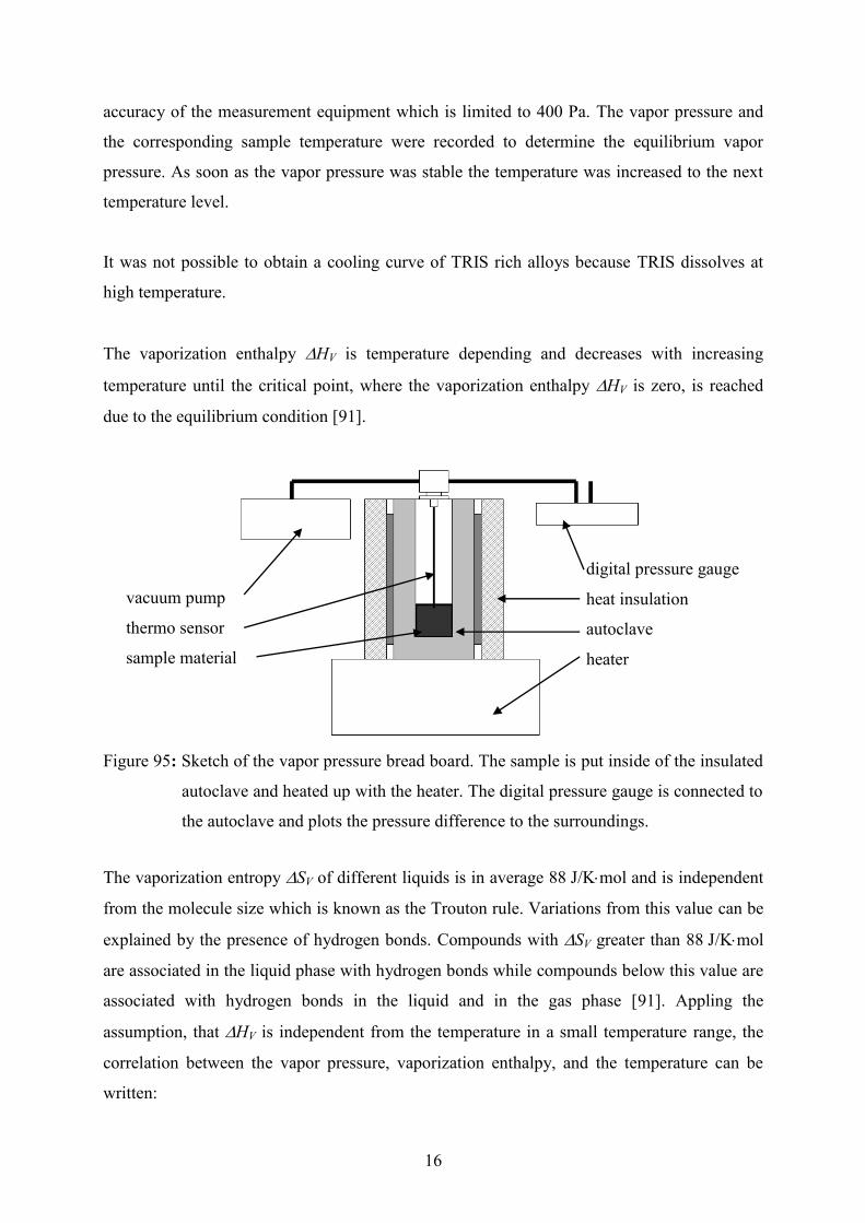
16
accuracy of the measurement equipment which is limited to 400 Pa. The vapor pressure and
the corresponding sample temperature were recorded to determine the equilibrium vapor
pressure. As soon as the vapor pressure was stable the temperature was increased to the next
temperature level.
It was not possible to obtain a cooling curve of TRIS rich alloys because TRIS dissolves at
high temperature.
The vaporization enthalpy HV is temperature depending and decreases with increasing
temperature until the critical point, where the vaporization enthalpy HV is zero, is reached
due to the equilibrium condition [91].
Figure 95: Sketch of the vapor pressure bread board. The sample is put inside of the insulated
autoclave and heated up with the heater. The digital pressure gauge is connected to
the autoclave and plots the pressure difference to the surroundings.
The vaporization entropy SV of different liquids is in average 88 J/Kmol and is independent
from the molecule size which is known as the Trouton rule. Variations from this value can be
explained by the presence of hydrogen bonds. Compounds with SV greater than 88 J/Kmol
are associated in the liquid phase with hydrogen bonds while compounds below this value are
associated with hydrogen bonds in the liquid and in the gas phase [91]. Appling the
assumption, that HV is independent from the temperature in a small temperature range, the
correlation between the vapor pressure, vaporization enthalpy, and the temperature can be
written:
vacuum pump
thermo sensor
sample material
digital pressure gauge
heat insulation
autoclave
heater

17
.1
ln constTR
Hp V
(Eq.20)
This equation can be transformed to a simple equation of first order where the slope
multiplied by the gas constant R is equal to the enthalpy HV. The correlation equation for the
vapor pressure of NPG is available from the chemical engineering research center (CHERIC)
[92], which is given by:
.10967256.999825.73162.5250
)ln(023658.9)ln( 26 TT
Tp (Eq. 21)
Here, p is the vapor pressure. Basic information about the vapor pressure at room temperature
of the pure compounds TRIS and NPG is available from material data sheets [93, 94]. Both
pure compounds are not mixable at room temperature, therefore, the entire vapor pressure can
be calculated from the partial vapor pressure of the pure compounds. According to Raoult’s
law [91] the vapor pressure p of an ideal solution is dependent on the vapor pressure of each
chemical component pA and pB and the mole fraction of the component xA and xB as shown in:
.BBAA xpxpp (Eq. 22)
Here, pA is partial pressure of the substance A and xA the mol fraction of substance A. Figure
96 shows the total vapor pressure of alloys at room temperature (293.15 K) depending on the
mol fraction. For more details at low temperature Front et al. [95] reported the pressure –
temperature equilibrium curve at the solid state for NPG. Further information about the molar
volume changes of NPG and TRIS at atmospheric pressure and pressure – temperature
dependencies for the phase transitions of compounds can be found in Tamarit [63].
Thermodynamic data for both compounds were reported at Sturz et al. [52].

18
0.0 0.2 0.4 0.6 0.8 1.0
0.0
0.1
0.2
0.3
0.4
p [P
a]
x
total vapor pressure TRIS - NPG
partial vapor pressure TRIS
partial vapor pressure NPG
TRIS NPG
Figure 96: The total vapor pressure of TRIS – NPG (black line) at room temperature
depending on the alloy concentration. NPG (red dots) has a 10 times higher
vapor pressure as TRIS (blue dots) and as a consequence the total vapor pressure
is more or less equal to the partial vapor pressure of pure NPG.
Table 16 gives the physical and chemical properties online available from material safety data
sheets of different producers.
Table 16: Material data
Material data
TRIS NPG
formula H2NC(CH2OH)3 (CH3)2C(CH2OH)2
Tm (melting) 442.7 1.0 K 401.3 1.0 K
Tb (as delivered) 492 – 493 K (at 13 hPa) [49] 481 – 482 K [49]
vapor pressure at 293 K 2.9 10-3
Pa [93] 100 Pa [94]
vapor pressure 1300 Pa at 492 K [96] 101.3 kPa at 482 K [97]
HSST 34.0 1.7 kJ/mol [52] 12.8 0.6 kJ/mol [52]
Hm 3.7 0.2 kJ/mol [52] 4.4 0.2 kJ/mol [52]
To check the experimental results, the vapor pressure equation of NPG from CHERIC [92]
was used as a reference. Figure 97 compares the experimental values with the calculated
values of NPG. A sufficient determination of the vapor pressure at room temperature was not
possible since the pressure was below the accuracy of the measurement instrument.

19
300 350 400 450 5000
40
80
120
160
200
gasliquid
Pre
ssu
re [
kP
a]
Temperature [K]
measured vapor presser
calculated vapor pressure
Neopenthylclycol
solid
Figure 97: Comparison of the measured vapor pressure of pure NPG (red dots) and the
calculated one (black line) available from “CHERIC” (chemical engineering
research center [92]). The experimental results show a slightly higher vapor
pressure in the solid and parts of the liquid state than calculated.
Results
To enhance the accuracy of the regression analysis the vapor pressure at room temperature has
been additionally calculated from equation 27 (see Figure 96). The relation between the
logarithm of the vapor pressure and the reciprocal of the temperature is shown in Figure 98
for a sample with a concentration of x = 0.7 mol fraction NPG.

20
0.002 0.003 0.004-12
-8
-4
0
4
ln (
p)
1/Temperature [1/K]
experimental results
linear fitting
calculated value
Figure 98: Natural logarithm of the vapor pressure at a temperature of 293 K, 475 K, 478 K
and 505 K at a concentration of x = 0.7 mol fraction NPG. The dotted line is the
regression analysis for the vapor pressure.
The average value of pressure and temperature was taken from experimental results of the
vapor pressure at the same temperature (± 2 °K) for the regression analysis. Table 17 gives
values of the regression analysis for different investigated concentrations.
Table 17: Results of the regression analysis.
C0 x Equation
mol.% NPG mol fraction
0 0 7.261
11589ln T
p
30 0.3 7.211
7.9129ln T
p
50 0.5 7.231
9.9584ln T
p
70 0.7 3.241
9.9621ln T
p
100 1 9.231
0.9368ln T
p
HV (in [J]) was calculated by multiplying the results given in Table 18 with the gas constant
R. From these values the average values and the deviations have been calculated and plotted
in Table 18 together with the phase transition enthalpies published in [52]. To estimate an
error bar for NPG, average and deviation of the experimental and the calculated results have
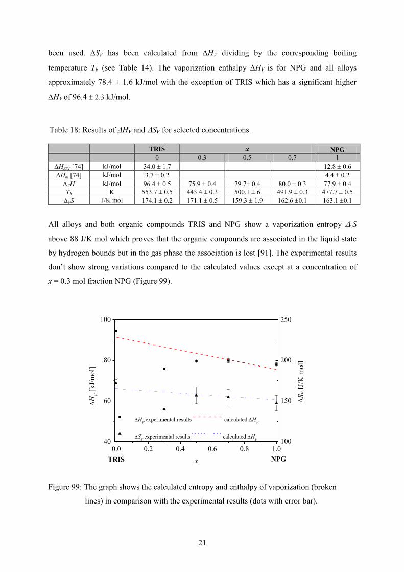
21
been used. SV has been calculated from HV dividing by the corresponding boiling
temperature Tb (see Table 14). The vaporization enthalpy HV is for NPG and all alloys
approximately 78.4 ± 1.6 kJ/mol with the exception of TRIS which has a significant higher
HV of 96.4 2.3 kJ/mol.
Table 18: Results of HV and SV for selected concentrations.
TRIS x NPG
0 0.3 0.5 0.7 1
HSST [74] kJ/mol 34.0 1.7 12.8 0.6
Hm [74] kJ/mol 3.7 0.2 4.4 0.2
VH kJ/mol 96.4 0.5 75.9 0.4 79.7 0.4 80.0 0.3 77.9 0.4
Tb K 553.7 ± 0.5 443.4 ± 0.3 500.1 ± 6 491.9 ± 0.3 477.7 ± 0.5
VS J/K mol 174.1 0.2 171.1 0.5 159.3 1.9 162.6 0.1 163.1 0.1
All alloys and both organic compounds TRIS and NPG show a vaporization entropy vS
above 88 J/K mol which proves that the organic compounds are associated in the liquid state
by hydrogen bounds but in the gas phase the association is lost [91]. The experimental results
don’t show strong variations compared to the calculated values except at a concentration of
x = 0.3 mol fraction NPG (Figure 99).
0.0 0.2 0.4 0.6 0.8 1.040
60
80
100
100
150
200
250
SV [
J/K
mo
l]
NPG
H
V [
kJ/
mo
l]
x
HV experimental results calculated H
V
SV experimental results calculated H
V
TRIS
Figure 99: The graph shows the calculated entropy and enthalpy of vaporization (broken
lines) in comparison with the experimental results (dots with error bar).
S
V [
J/K
mol]
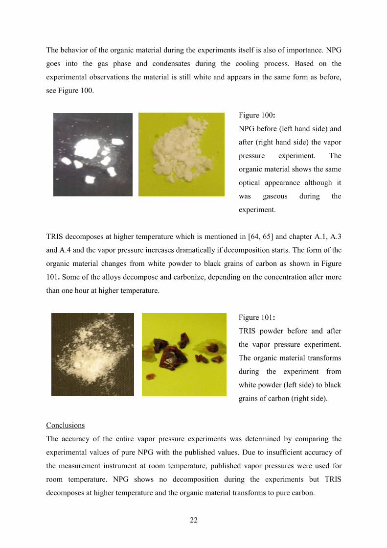
22
The behavior of the organic material during the experiments itself is also of importance. NPG
goes into the gas phase and condensates during the cooling process. Based on the
experimental observations the material is still white and appears in the same form as before,
see Figure 100.
Figure 100:
NPG before (left hand side) and
after (right hand side) the vapor
pressure experiment. The
organic material shows the same
optical appearance although it
was gaseous during the
experiment.
TRIS decomposes at higher temperature which is mentioned in [64, 65] and chapter A.1, A.3
and A.4 and the vapor pressure increases dramatically if decomposition starts. The form of the
organic material changes from white powder to black grains of carbon as shown in Figure
101. Some of the alloys decompose and carbonize, depending on the concentration after more
than one hour at higher temperature.
Figure 101:
TRIS powder before and after
the vapor pressure experiment.
The organic material transforms
during the experiment from
white powder (left side) to black
grains of carbon (right side).
Conclusions
The accuracy of the entire vapor pressure experiments was determined by comparing the
experimental values of pure NPG with the published values. Due to insufficient accuracy of
the measurement instrument at room temperature, published vapor pressures were used for
room temperature. NPG shows no decomposition during the experiments but TRIS
decomposes at higher temperature and the organic material transforms to pure carbon.
23
The vaporization enthalpy HV for NPG and all alloys is approximately 78.4 ± 1.6 kJ/mol
with the exception of TRIS which has a significant higher HV of 96.4 2.3 kJ/mol. All alloys
and both organic compounds TRIS and NPG show a vaporization entropy vS above 88 J/K
mol which proves that the organic compounds are associated in the liquid state by hydrogen
bounds but in the gas phase the association is lost [91].
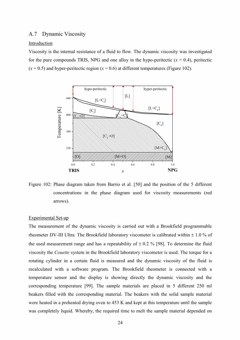
24
A.7 Dynamic Viscosity
Introduction
Viscosity is the internal resistance of a fluid to flow. The dynamic viscosity was investigated
for the pure compounds TRIS, NPG and one alloy in the hypo-peritectic (x = 0.4), peritectic
(x = 0.5) and hyper-peritectic region (x = 0.6) at different temperatures (Figure 102).
0.0 0.2 0.4 0.6 0.8 1.0
320
360
400
440
NPG
Tem
per
ature
[K
]
x
[L]
hypo-peritectic hyper-peritectic
[L+Cl]
[L+CF]
[CF+C
l]
[Cl]
[Cl+O]
[CF+O]
[CF]
[M+CF]
[M+O][O] [M]
TRIS
Figure 102: Phase diagram taken from Barrio et al. [50] and the position of the 5 different
concentrations in the phase diagram used for viscosity measurements (red
arrows).
Experimental Set-up
The measurement of the dynamic viscosity is carried out with a Brookfield programmable
rheometer DV-III Ultra. The Brookfield laboratory viscometer is calibrated within 1.0 % of
the used measurement range and has a repeatability of 0.2 % [98]. To determine the fluid
viscosity the Couette system in the Brookfield laboratory viscometer is used. The torque for a
rotating cylinder in a certain fluid is measured and the dynamic viscosity of the fluid is
recalculated with a software program. The Brookfield rheometer is connected with a
temperature sensor and the display is showing directly the dynamic viscosity and the
corresponding temperature [99]. The sample materials are placed in 5 different 250 ml
beakers filled with the corresponding material. The beakers with the solid sample material
were heated in a preheated drying oven to 453 K and kept at this temperature until the sample
was completely liquid. Whereby, the required time to melt the sample material depended on

25
the concentration. For pure NPG it takes about 1 hour, for the 3 alloys approximately 2 hours,
and for pure TRIS 3 hours. To avoid vaporization during the melting process the beakers were
sealed with glass and foil. All experiments were carried out under normal atmospheric
conditions in a gas hood since there was no glove box available with an adequate size to host
the necessary equipment. The beaker with the liquid sample material was placed on a hot
laboratory heater and protected with glass padding and a foil to avoid cooling from the top as
shown in Figure 103.
Figure 103: The experimental arrangement for the estimation of the dynamic viscosity. The
beaker is completely protected by glass padding and a foil.
The temperature sensor and the rotation cylinder from the viscometer are put into the fluid.
The fluid in the beaker was stirred to establish a homogeneous temperature field. As soon as
the temperature field is stabilized, the stirring of the liquid alloy is stopped for the
measurement. Subsequently the temperature is reduced in discrete steps to measure the
viscosity. It was not possible to establish a homogeneous temperature field below 410 K
because the material solidified too fast.
Results
Concentrations between 0.4 x 0.6 mol fraction NPG were selected because the
investigations for peritectic solidification with the DIRSOL instrument under 1 µg condition
will be carried out with alloys in this concentration range. Viscous flow in amorphous
materials like glasses or melts is a thermal activated process and depends on the Arrhenius-
Andrade equation [91]:
isolation foil
glass padding
temperature sensor
sample material
Brookfield Programmable
Rheometer DV-III Ultra
Beaker
bob and rotating cylinder
with protection cage
laboratory heater
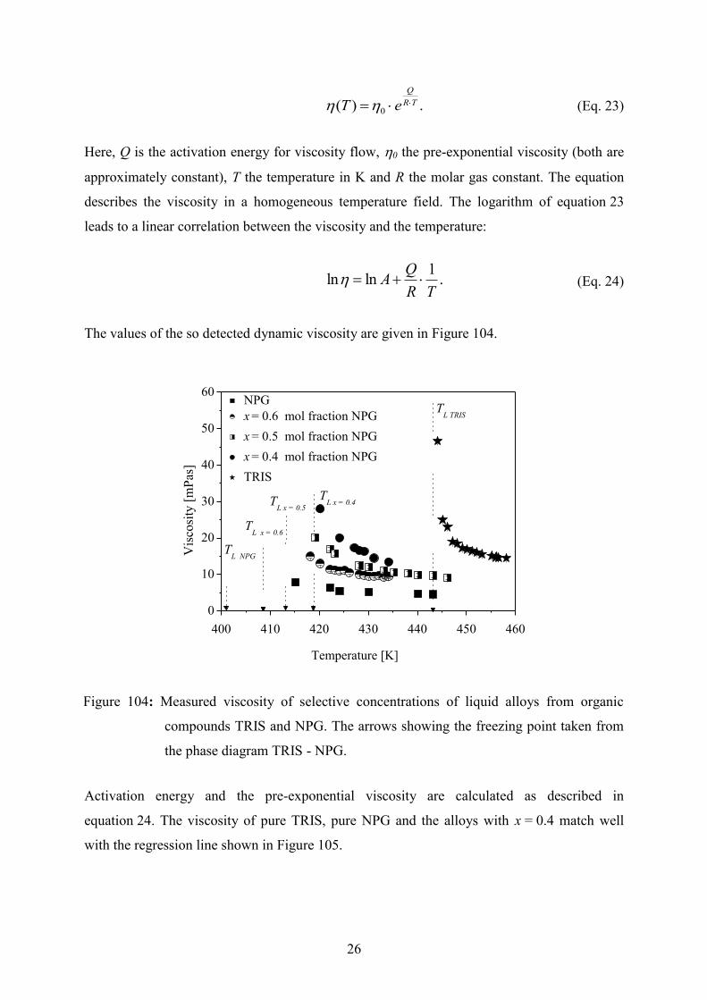
26
.)( 0TR
Q
eT (Eq. 23)
Here, Q is the activation energy for viscosity flow, 0 the pre-exponential viscosity (both are
approximately constant), T the temperature in K and R the molar gas constant. The equation
describes the viscosity in a homogeneous temperature field. The logarithm of equation 23
leads to a linear correlation between the viscosity and the temperature:
.1
lnlnTR
QA (Eq. 24)
The values of the so detected dynamic viscosity are given in Figure 104.
400 410 420 430 440 450 460
0
10
20
30
40
50
60
TL TRIS
TL x = 0.4
TL x = 0.5
TL x = 0.6
Vis
cosi
ty [
mP
as]
Temperature [K]
NPG
x = 0.6 mol fraction NPG
x = 0.5 mol fraction NPG
x = 0.4 mol fraction NPG
TRIS
TL NPG
Figure 104: Measured viscosity of selective concentrations of liquid alloys from organic
compounds TRIS and NPG. The arrows showing the freezing point taken from
the phase diagram TRIS - NPG.
Activation energy and the pre-exponential viscosity are calculated as described in
equation 24. The viscosity of pure TRIS, pure NPG and the alloys with x = 0.4 match well
with the regression line shown in Figure 105.
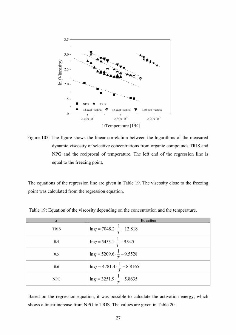
27
2.20x10⁻³
2.30x10⁻³
2.40x10⁻³
1.0
1.5
2.0
2.5
3.0
3.5
ln (
Vis
cosi
ty)
1/Temperature [1/K]
NPG TRIS
0.6 mol fraction 0.5 mol fraction 0.40 mol fraction
Figure 105: The figure shows the linear correlation between the logarithms of the measured
dynamic viscosity of selective concentrations from organic compounds TRIS and
NPG and the reciprocal of temperature. The left end of the regression line is
equal to the freezing point.
The equations of the regression line are given in Table 19. The viscosity close to the freezing
point was calculated from the regression equation.
Table 19: Equation of the viscosity depending on the concentration and the temperature.
x Equation
TRIS 818.121
2.7048ln T
0.4 945.91
1.5453ln T
0.5 5528.91
6.5209ln T
0.6 8165.81
4.4781ln T
NPG 8635.51
9.3251ln T
Based on the regression equation, it was possible to calculate the activation energy, which
shows a linear increase from NPG to TRIS. The values are given in Table 20.

28
Table 20: Activation energy and viscosity close to the melting point of the organic material
and their alloys.
x Q (close to the melting point)
mol fraction kJ/mol m∙Pa∙s
TRIS 58.6 22.3
0.4 45.3 21.8
0.5 43.3 21.2
0.6 39.7 17.9
NPG 27.0 9.4
The determination of the viscosity is based on one experiment for each concentration.
Normally, the accuracy of experiments can be calculated from the deviation of the average
value. In this case, it’s not possible, therefore, the published values of NEOL [100], a trade
mark for NPG of the company BASF, are used as reference material instead. It has to be
mentioned that both materials, NEOL from BASF and NPG from Aldrich, have the same CAS
number but not exact the same contents. Figure 106 compares the viscosity of NEOL and the
experimental results with NPG.
2.25x10⁻³
2.30x10⁻³
2.35x10⁻³
2.40x10⁻³
2.45x10⁻³
2.50x10⁻³
0.0
0.5
1.0
1.5
2.0
2.5
3.0
3.5
ln (V
iscosity)
1/Temperature [1/K]
NPG
NEOL
freezing point
Figure 106: The graph shows the experimental results of pure NPG and the published values
of NEOL a trade mark from BASF. The viscosity at the freezing point is for both
materials calculated from the regression line.
The viscosity at the freezing point is calculated for both materials. Here, the vales show good
agreement whereas with rising temperature the viscosity of both materials diverges more and
more.

29
Conclusions
The values of the dynamic viscosity increase from pure NPG to pure TRIS. The determination
of the viscosity close to the freezing point was not possible for all selected concentrations
since a measurement below 410 K failed, because of the applied process conditions. From the
regression equation, it was possible to calculate the viscosity shortly before the liquid starts to
freeze. The experimental values for the viscosity are used to estimate the diffusion coefficient.
The accuracy of the values is checked by the comparison of published values and
experimental ones.

30
A.8 Temperature Gradient
Due to the difference in the heat conductivity of solid and liquid and to the evolution of latent
heat at a moving interface, the temperature gradient in the liquid may generally not be equal
to the gradient in the solid. The temperature gradient [2] is given in the form,
LS
LLSST
GGG
. (Eq. 25)
Here, GS is the temperature gradient in the solid, S the thermal conductivity in the solid, GL
the temperature gradient in the liquid, and L the thermal conductivity in the liquid.
[75] published the thermal conductivity ratio of equilibrated liquid phase to solid phase for
NPG with 1.07. Since the difference between LandS (0.185 and 0.184 [81, 82]) is small
for the peritectic concentration of our system, the temperature gradient for the TRIS – NPG
system can be assumed to be GT GL.
Experimental Set-up
The measurement of the temperature gradient within the adiabatic zone requires a temperature
sensor which fits into the size of the glass samples. However, the used long rectangle glass
samples of the solidification experiments have to be very thin (100 µm thickness) to reduce
the influence of the convection as much as possible. The width and the long length of the
glass sample prevent the usage of thermocouples with smaller diameters, like 20 µm.
Therefore, the selected special sample size disables the application of a suitable temperature
sensor. To measure the temperature gradient, a larger glass sample (0.8 x 3.5 mm2 instead of
0.1 x 2.0 mm2) is used, filled with a sample of peritectic concentration. An additional adapter
has to be used to fit the larger sample into the Bridgman-furnace.
Ni-CrNi thermocouples, type K, were used with a diameter of 200 µm in order to evaluate the
temperature gradient between the hot and the cold part of the Bridgman-furnace. Two
thermocouples were put into a rectangular sample (0.8 x 3.5 mm2) with a distance of
approximately 200 µm. The Bridgman furnace was preheated up to TH = 453 ± 1 K and
TC = 353 ± 1 K because (i) the temperature of the hot zone is limited due to the detected
thermal instability of TRIS (by DSC measurement, see Figure 32), and (ii) the interface
should be right in the center of the gap. The sample was placed in the furnace and was moved
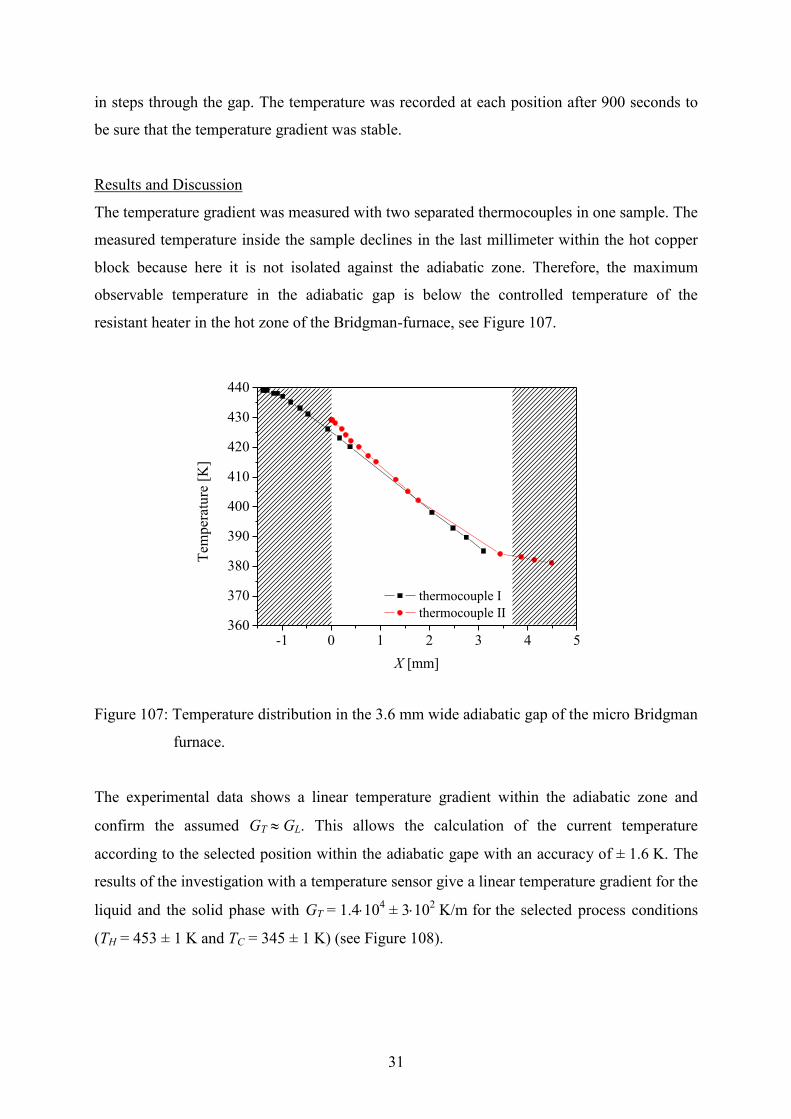
31
in steps through the gap. The temperature was recorded at each position after 900 seconds to
be sure that the temperature gradient was stable.
Results and Discussion
The temperature gradient was measured with two separated thermocouples in one sample. The
measured temperature inside the sample declines in the last millimeter within the hot copper
block because here it is not isolated against the adiabatic zone. Therefore, the maximum
observable temperature in the adiabatic gap is below the controlled temperature of the
resistant heater in the hot zone of the Bridgman-furnace, see Figure 107.
-1 0 1 2 3 4 5360
370
380
390
400
410
420
430
440
Tem
per
atu
re [
K]
X [mm]
thermocouple I
thermocouple II
Figure 107: Temperature distribution in the 3.6 mm wide adiabatic gap of the micro Bridgman
furnace.
The experimental data shows a linear temperature gradient within the adiabatic zone and
confirm the assumed GT GL. This allows the calculation of the current temperature
according to the selected position within the adiabatic gape with an accuracy of ± 1.6 K. The
results of the investigation with a temperature sensor give a linear temperature gradient for the
liquid and the solid phase with GT = 1.4104 ± 310
2 K/m
for
the selected process conditions
(TH = 453 ± 1 K and TC = 345 ± 1 K) (see Figure 108).

32
0 1 2 3 4340
360
380
400
420
440
T =427.98087-14.16175 X
X [mm]
Tem
per
atu
re [
K]
results
fit
Figure 108: Linear fitting of the temperature field in the gap of the Bridgman furnace.
With the known temperature gradient the current interface temperature of the solid/liquid can
be detected, see Figure 109.
Figure 109: Picture of a sample in a temperature gradient field. The position of the planar
solid/liquid (TL) and solid/solid transformation front (TS) can be clearly
differentiated.
T
X
GT TL
TS

33
A.9 Diffusion Coefficient
Introduction
The organic peritectic phase diagram TRIS – NPG is used as a model system for in-situ
observation of layered structures where one or both phases, the primary and the peritectic
phase, solidify as a planar front solid/liquid interface. The liquid diffusion coefficient DL is
needed to analyze the solidification morphology. Liu et al. [101] published a suitable
experimental investigation for in-situ observation to determinate the diffusion coefficient in
the liquid. Liquid inclusions, like droplets, can moves in a solid matrix within an existing
temperature gradient GT. The movement, caused by the melting of the solid in contact with the
liquid at the hotter temperature and the solidification of the liquid in contact with the solid on
the colder temperature side of the liquid. The movement ends at the solid/liquid interface.
Melting and solidification within the temperature gradient creates a characteristic migration
curve depending on the diffusion coefficient in the liquid. From this characteristic curve it is
possible to calculate the diffusion coefficient for a given concentration. Liu et al. [101] shows
that the diffusion coefficient DL can be calculated from the coefficient a of the quadratic
polynomial velocity curve with:
ctxbtxat )()( 2 . (Eq. 26)
Here, t is the time of the droplet to move through the solid matrix to the solid/liquid interface,
a, b and c are coefficients, and x(t) the time depending position of the droplet in the matrix.
The diffusion coefficient is given by:
L
SL
G
G
a
kD
2
1. (Eq. 27)
Here, a is the coefficient from the migration curve.
Experimental Set-up
The experimental set-up in the Bridgman-furnace is described in chapter 3.1.1 and chapter 3.2
in more detail. The micro Bridgman-furnace is preheated and a glass sample with a selected
concentration is put into the furnace. Within the temperature gradient the solid alloy melts and
forms a planar solid/liquid interface. Afterwards the sample is pulled with 115 µm/s where

34
only dendrites with small dendrite arm spacing, 1, can grow, see Figure 110. During the
growth, the liquid is trapped between the side arms of the dendrites. Depending on the
selected concentration, the matrix of the phase corresponds to the [Cl] or [CF] phase.
Figure 110: Growth of a dendritic solidification front. On the right side of the picture, the
initial planar solid/liquid interface is visible.
After a few seconds the sample is stopped and stays unmoved within the Bridgman-furnace.
Now, the dendritic solid/liquid interface changes into a planar front and the entrapped liquid
forms droplets. This droplets start to move through the solid matrix, see Figure 111.
Figure 111: Picture of the organic alloy TRIS - NPG with a mol fraction of x = 0.4 mol
fraction NPG in rest. The bubbles are moving from the cold right side to the hot
left side and disappear at the solid/liquid interface.
The movement takes placed in such a way that one side of the droplet melts whereby the
opposite side solidifies simultaneously. For the calculation of the diffusion coefficient in the
liquid, the position with time is recorded for selected droplets.
[L] [] dendrites
trapped [L]
[L]
[] solid matrix
[] liquid inclusions
100 µm
100 µm
initial planar front
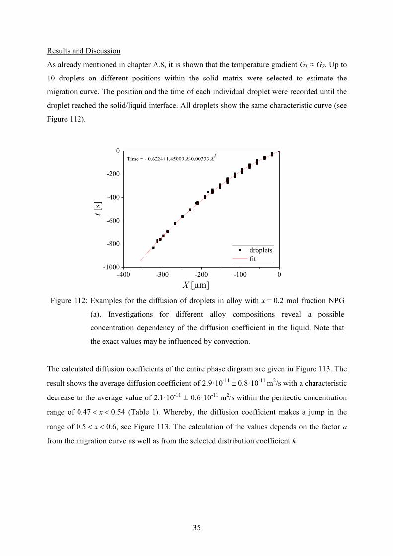
35
Results and Discussion
As already mentioned in chapter A.8, it is shown that the temperature gradient GL ≈ GS. Up to
10 droplets on different positions within the solid matrix were selected to estimate the
migration curve. The position and the time of each individual droplet were recorded until the
droplet reached the solid/liquid interface. All droplets show the same characteristic curve (see
Figure 112).
-400 -300 -200 -100 0-1000
-800
-600
-400
-200
0
t [s
]
Time = - 0.6224+1.45009 X-0.00333 X2
X [µm]
droplets
fit
Figure 112: Examples for the diffusion of droplets in alloy with x = 0.2 mol fraction NPG
(a). Investigations for different alloy compositions reveal a possible
concentration dependency of the diffusion coefficient in the liquid. Note that
the exact values may be influenced by convection.
The calculated diffusion coefficients of the entire phase diagram are given in Figure 113. The
result shows the average diffusion coefficient of 2.9·10-11
0.8·10-11
m2/s with a characteristic
decrease to the average value of 2.1·10-11
0.6·10-11
m2/s within the peritectic concentration
range of 0.47 x 0.54 (Table 1). Whereby, the diffusion coefficient makes a jump in the
range of 0.5 x 0.6, see Figure 113. The calculation of the values depends on the factor a
from the migration curve as well as from the selected distribution coefficient k.

36
0.0 0.2 0.4 0.6 0.8 1.00.0
2.0x10⁻¹¹
4.0x10⁻¹¹
6.0x10⁻¹¹
Dif
fusi
on c
oef
fici
ent
[m2/s
]
x [mol fraction]
peritectic plateau
average
diffusion coefficient
Figure 113: The derived diffusion coefficients DL plotted versus the alloy concentration.
Whereas, the estimated factor a from the migration curve is independent from the phase
diagram and only a mathematical factor. Besides, the used distribution coefficient k depends
on the selected phase diagram. Diffusion in the liquid depends on the temperature, the size of
the molecules and on the phase that solidifies. During solidification the rejected element
enriches in the liquid layer ahead of the solidification front, this behavior is reflected in the
distribution coefficient k. In the phase diagram TRIS - NPG within the range of 0.4 x 0.8
mol fraction the distribution coefficient k is nearly consistent. In alloys close to pure elements
only few host elements are present which makes diffusion easier. The estimated values of DL
are shown in Table 6 on page 40.
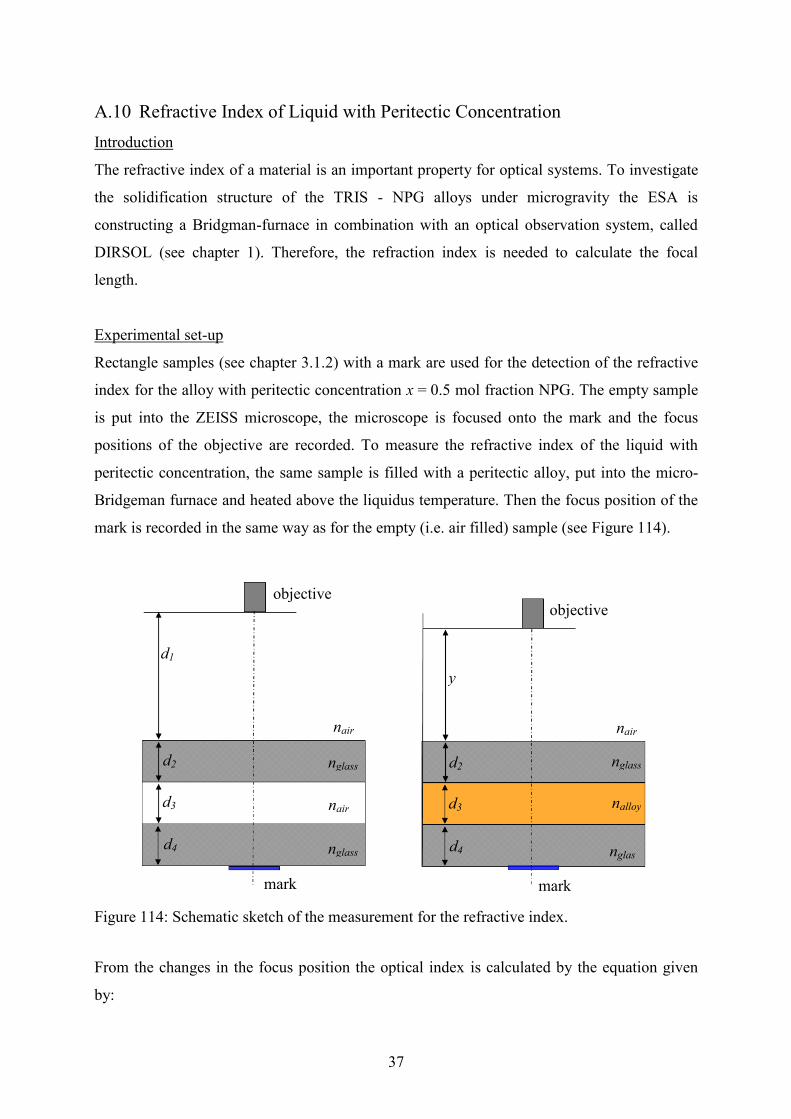
37
A.10 Refractive Index of Liquid with Peritectic Concentration
Introduction
The refractive index of a material is an important property for optical systems. To investigate
the solidification structure of the TRIS - NPG alloys under microgravity the ESA is
constructing a Bridgman-furnace in combination with an optical observation system, called
DIRSOL (see chapter 1). Therefore, the refraction index is needed to calculate the focal
length.
Experimental set-up
Rectangle samples (see chapter 3.1.2) with a mark are used for the detection of the refractive
index for the alloy with peritectic concentration x = 0.5 mol fraction NPG. The empty sample
is put into the ZEISS microscope, the microscope is focused onto the mark and the focus
positions of the objective are recorded. To measure the refractive index of the liquid with
peritectic concentration, the same sample is filled with a peritectic alloy, put into the micro-
Bridgeman furnace and heated above the liquidus temperature. Then the focus position of the
mark is recorded in the same way as for the empty (i.e. air filled) sample (see Figure 114).
Figure 114: Schematic sketch of the measurement for the refractive index.
From the changes in the focus position the optical index is calculated by the equation given
by:
nglass d2
nglass
d1
d3
d4
nair
y
d2
d3
d4 nglas
nair nair
nglass
nalloy
mark mark
objective objective

38
.)(
3
31
432
4321
d
yddnn
ndndndny
ndndndnd
air
alloy
glassalloyglassair
glassairglassair
(Eq. 28)
Here, n is the refractive index, and d the inner dimension of the glass sample.
Results
The measurement of the refractive index n is repeated for air and water (are given in Table
21) to reduce the measurement error.
Table 21: Measured refractive index.
unit air water x = 0.5
mol fraction NPG
temperature measured K 293 293 443
n measured - 0.999 1.39 1.35
published [102] - 1.0003 1.33 -
Top Related