


Languages
Pages
Legal

WS2014/2015, 17.12.2014
Intelligent SystemsStatistical Machine Learning
Carsten Rother, Dmitrij Schlesinger
17.12.2014Intelligent Systems: Statistical Machine Learning 2
Our tasks (recap)
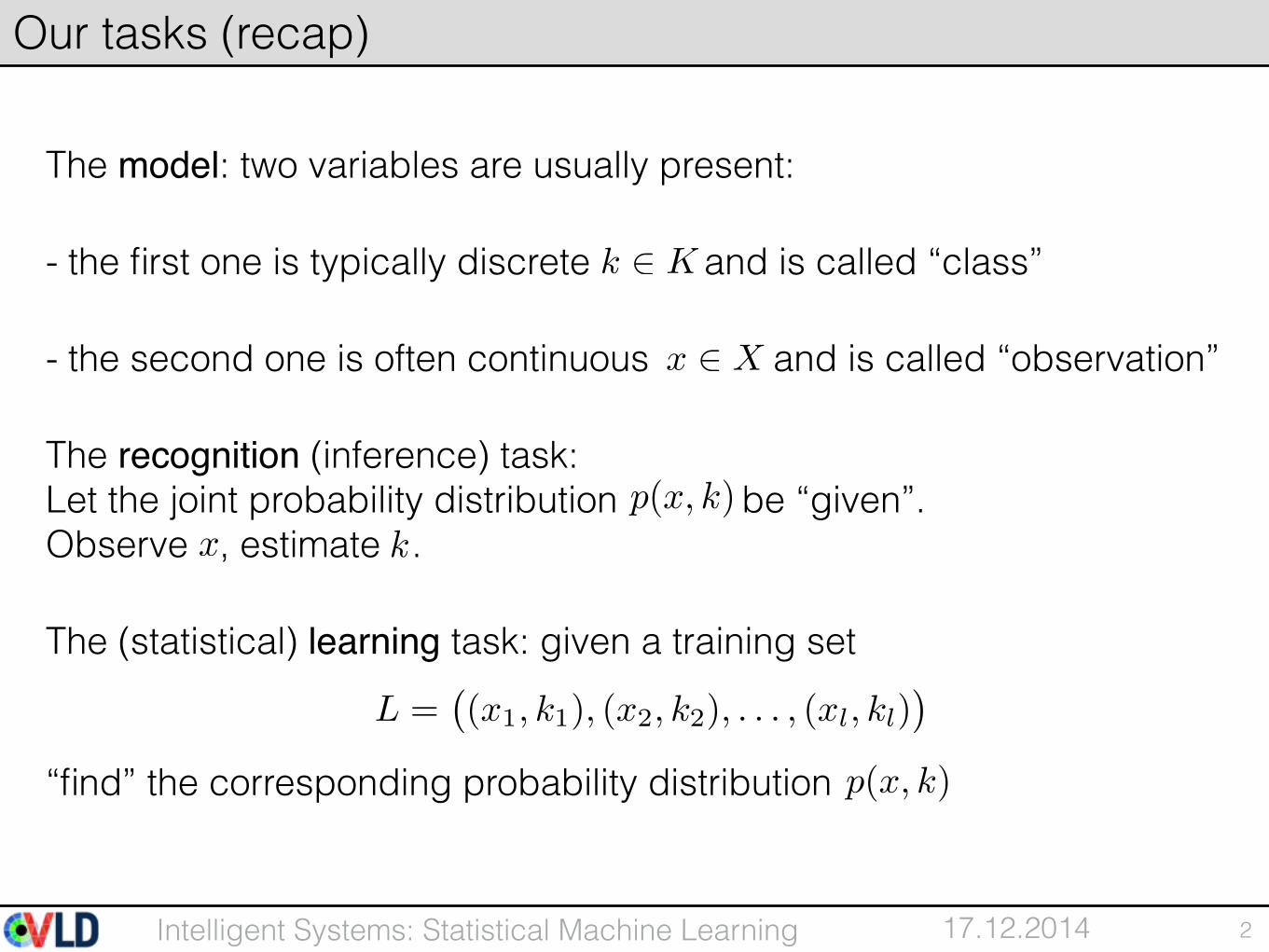
The model: two variables are usually present:
- the first one is typically discrete and is called “class”
- the second one is often continuous and is called “observation”
The recognition (inference) task: Let the joint probability distribution be “given”. Observe , estimate .
The (statistical) learning task: given a training set
“find” the corresponding probability distribution
k 2 K
x 2 X
p(x, k)x k
L =�(x1, k1), (x2, k2), . . . , (xl, kl)
�
p(x, k)
17.12.2014Intelligent Systems: Statistical Machine Learning
• Decision making:
• Bayesian Decision Theory
• Non-Bayesian formulation
• Statistical Learning — Maximum Likelihood Principle
3
Outline
17.12.2014Intelligent Systems: Statistical Machine Learning
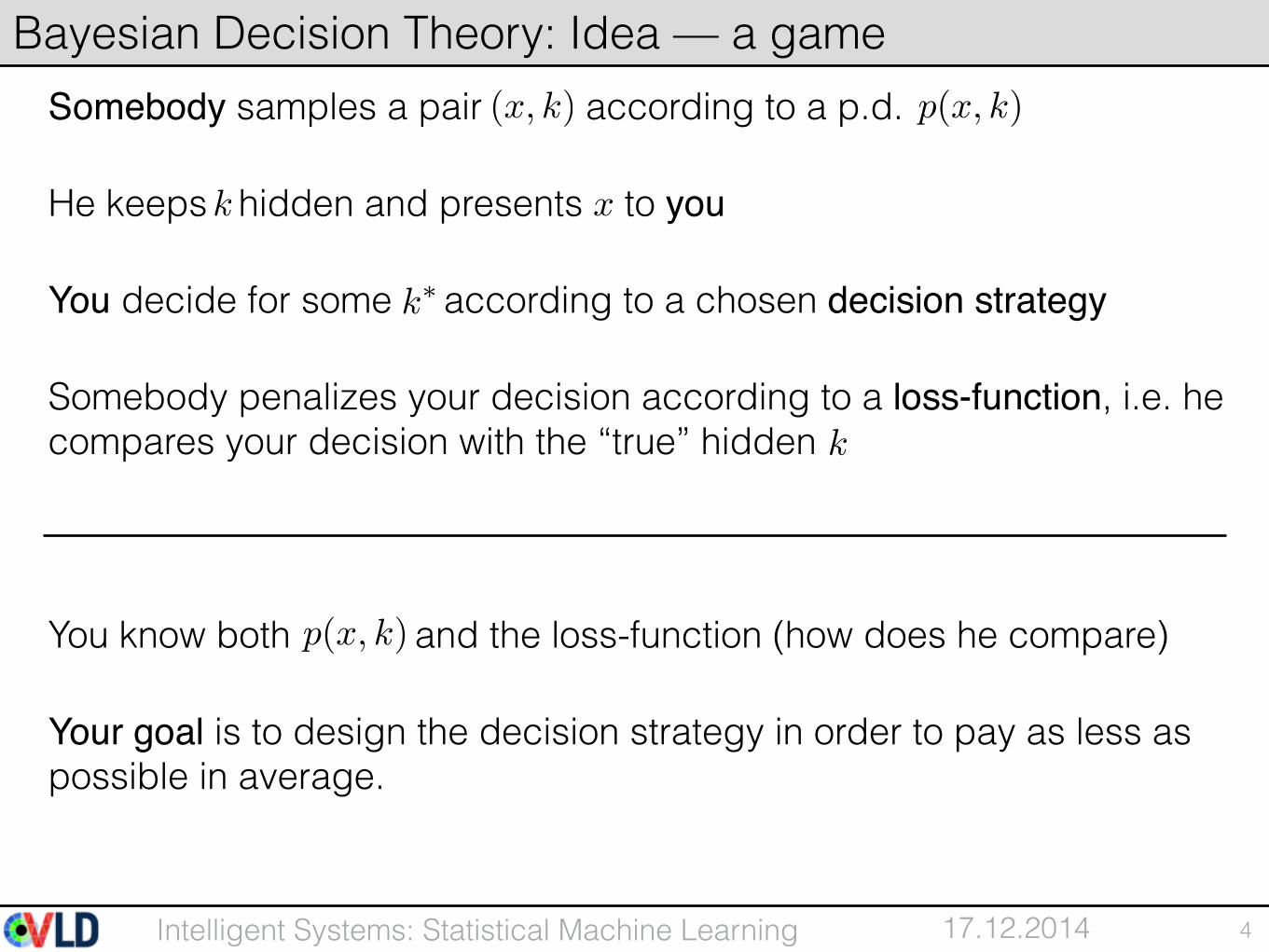
Somebody samples a pair according to a p.d.
He keeps hidden and presents to you
You decide for some according to a chosen decision strategy
Somebody penalizes your decision according to a loss-function, i.e. he compares your decision with the “true” hidden
You know both and the loss-function (how does he compare)
Your goal is to design the decision strategy in order to pay as less as possible in average.
4
Bayesian Decision Theory: Idea — a game(x, k) p(x, k)
k x
k⇤
k
p(x, k)
17.12.2014Intelligent Systems: Statistical Machine Learning
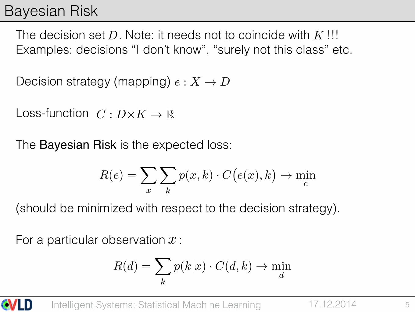
The decision set . Note: it needs not to coincide with !!! Examples: decisions “I don’t know”, “surely not this class” etc.
Decision strategy (mapping)
Loss-function
The Bayesian Risk is the expected loss:
(should be minimized with respect to the decision strategy).
For a particular observation :
5
Bayesian RiskD K
e : X ! D
C : D⇥K ! R
R(e) =X
x
X
k
p(x, k) · C�e(x), k
�! min
e
R(d) =X
k
p(k|x) · C(d, k) ! mind
x
17.12.2014Intelligent Systems: Statistical Machine Learning
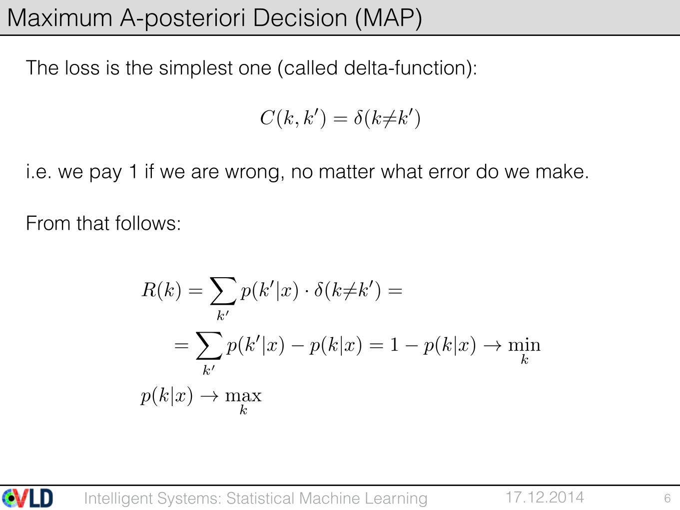
The loss is the simplest one (called delta-function):
i.e. we pay 1 if we are wrong, no matter what error do we make.
From that follows:
6
Maximum A-posteriori Decision (MAP)
C(k, k0) = �(k 6=k0)
R(k) =
X
k0
p(k
0|x) · �(k 6=k
0) =
=
X
k0
p(k
0|x)� p(k|x) = 1� p(k|x) ! min
k
p(k|x) ! max
k
17.12.2014Intelligent Systems: Statistical Machine Learning
The decision set is , i.e. it is extended by a special decision “I don’t know” (rejection). The loss-function is
i.e. we pay a (reasonable) penalty if we are lazy to decide.
Case-by-case analysis:
1. We decide for a class , decision is MAP , the loss for this is
2. We decide to reject , the loss for this is
The decision strategy: Compare with and decide for the variant with the greater value.
7
Decision with rejectionD = K [ {rw}
C(d, k) =
⇢�(k 6=k0) if d 2 K" if d = rw
d 2 K d = k⇤
1� p(k⇤|x)
d = rw "
! p(k⇤|x) 1� "
17.12.2014Intelligent Systems: Statistical Machine Learning
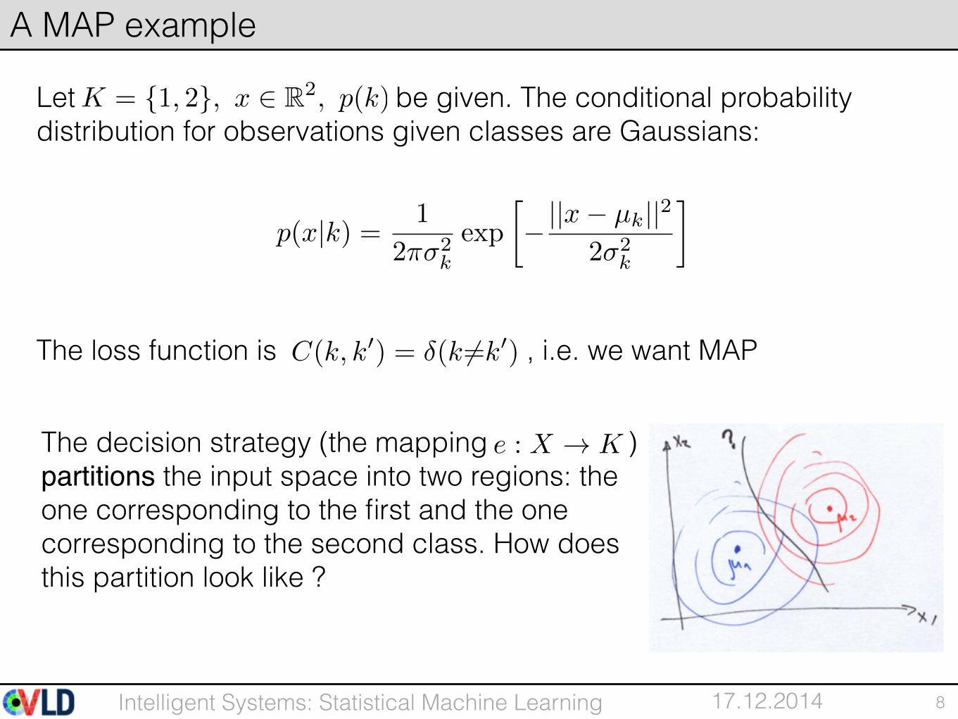
Let be given. The conditional probability distribution for observations given classes are Gaussians:
The loss function is , i.e. we want MAP
8
A MAP example
K = {1, 2}, x 2 R2, p(k)
p(x|k) = 1
2⇡�
2k
exp
� ||x� µk||2
2�
2k
�
C(k, k0) = �(k 6=k0)
The decision strategy (the mapping ) partitions the input space into two regions: the one corresponding to the first and the one corresponding to the second class. How does this partition look like ?
e : X ! K
17.12.2014Intelligent Systems: Statistical Machine Learning
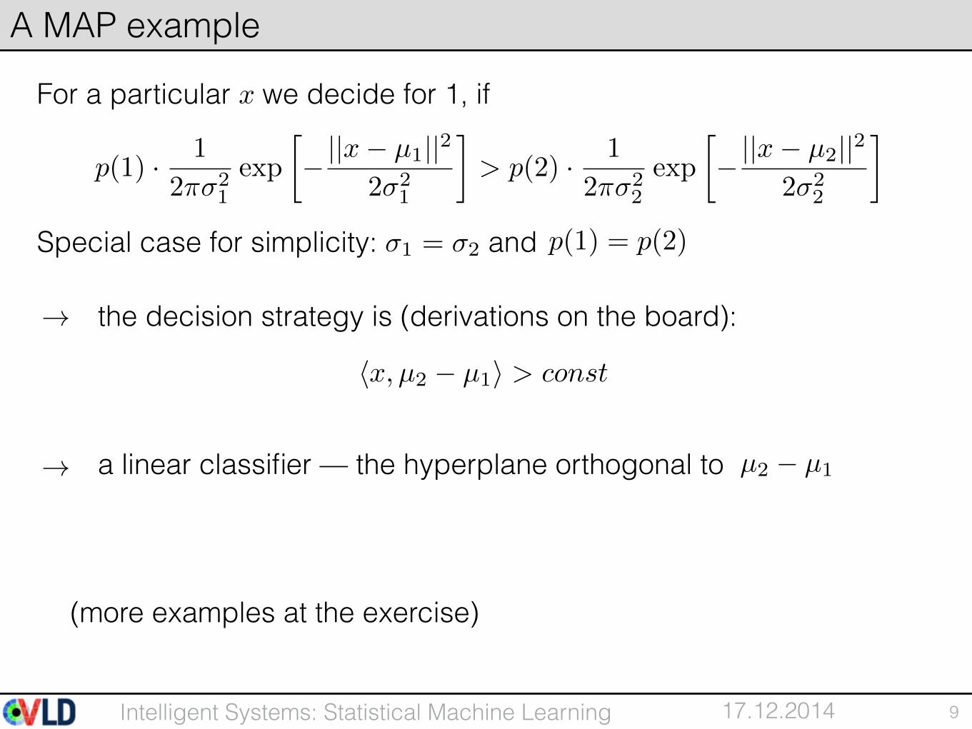
For a particular we decide for 1, if
Special case for simplicity: and
the decision strategy is (derivations on the board):
a linear classifier — the hyperplane orthogonal to
(more examples at the exercise)
9
A MAP example
p(1) · 1
2⇡�
21
exp
� ||x� µ1||2
2�
21
�> p(2) · 1
2⇡�
22
exp
� ||x� µ2||2
2�
22
�
�1 = �2 p(1) = p(2)
!
hx, µ2 � µ1i > const
µ2 � µ1!
x

17.12.2014Intelligent Systems: Statistical Machine Learning
• Decision making:
• Bayesian Decision Theory
• Non-Bayesian formulation
• Statistical Learning — Maximum Likelihood Principle
10
Outline
17.12.2014Intelligent Systems: Statistical Machine Learning
Despite the generality of Bayesian approach, there are many tasks which cannot be expressed within the Bayesian framework:
• It is difficult to establish a penalty function, e.g. it does not assume values from the totally ordered set.
• A priori probabilities are not known or cannot be known because is not a random event.
An example – Russian fairy tales hero
When he turns to the left, he loses his horse, when he turns to the right, he loses his sword, and if he turns back, he loses his beloved girl.
Is the sum of horses and swords is less or more than beloved girls ?
11
Non-Bayesian Decisions
p(k)k
p1 p2 p3
17.12.2014Intelligent Systems: Statistical Machine Learning
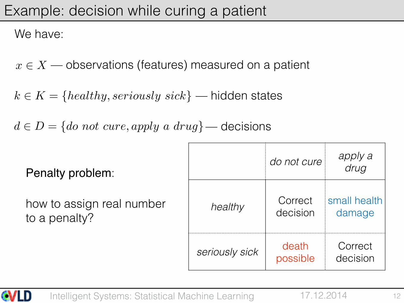
We have:
— observations (features) measured on a patient
— hidden states
— decisions
12
Example: decision while curing a patient
x 2 X
k 2 K = {healthy, seriously sick}
d 2 D = {do not cure, apply a drug}
do not cure apply a drug
healthy Correct decision
small health damage
seriously sick death possible
Correct decision
Penalty problem:
how to assign real number to a penalty?

17.12.2014Intelligent Systems: Statistical Machine Learning
Observation describes the observed airplane.
Two hidden states:
The conditional probability can depend on the observation in a complicated manner but it exists and describes dependencies of the observation on the situation correctly.
A-priori probabilities are not known and can not be known in principle.
the hidden state is not a random event
13
Example: enemy or allied airplane ?
x
⇢k = 1 allied airplanek = 2 enemy airplane
p(x|k) x
x k
p(k)
! k
17.12.2014Intelligent Systems: Statistical Machine Learning
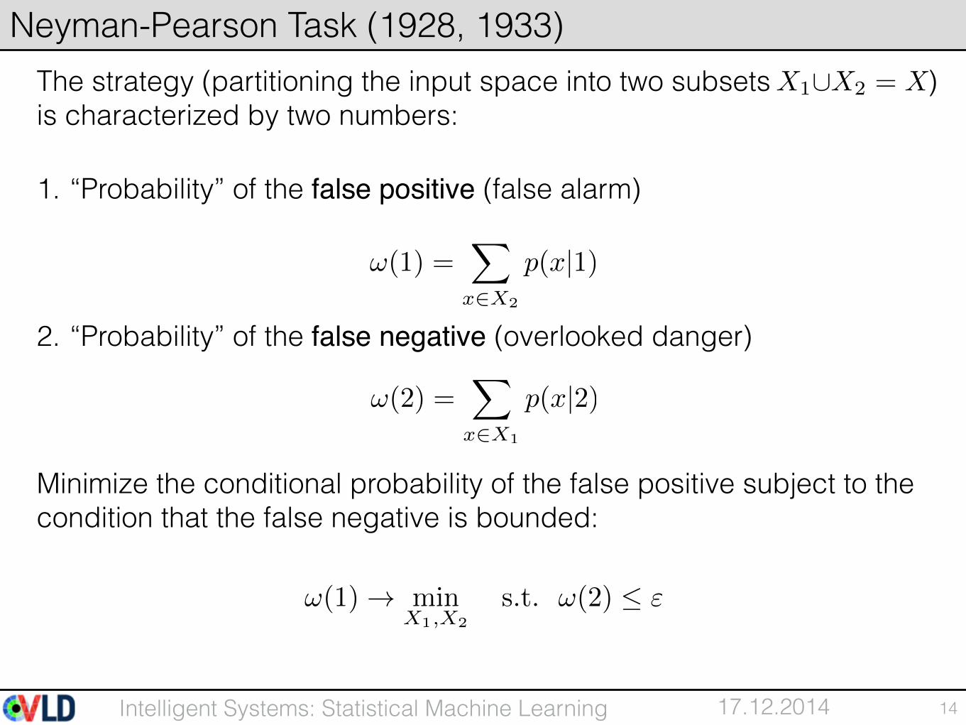
The strategy (partitioning the input space into two subsets ) is characterized by two numbers:
1. “Probability” of the false positive (false alarm)
2. “Probability” of the false negative (overlooked danger)
Minimize the conditional probability of the false positive subject to the condition that the false negative is bounded:
14
Neyman-Pearson Task (1928, 1933)
!(1) =X
x2X2
p(x|1)
!(2) =X
x2X1
p(x|2)
X1[X2 = X
!(1) ! minX1,X2
s.t. !(2) "
17.12.2014Intelligent Systems: Statistical Machine Learning
• Decision making:
• Bayesian Decision Theory
• Non-Bayesian formulation
• Statistical Learning — Maximum Likelihood Principle
15
Outline
17.12.2014Intelligent Systems: Statistical Machine Learning
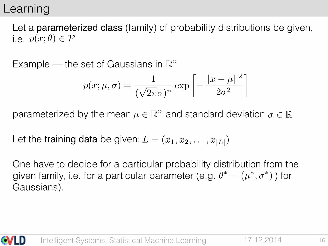
Let a parameterized class (family) of probability distributions be given, i.e.
Example — the set of Gaussians in
parameterized by the mean and standard deviation
Let the training data be given:
One have to decide for a particular probability distribution from the given family, i.e. for a particular parameter (e.g. ) for Gaussians).
16
Learning
p(x; ✓) 2 P
Rn
p(x;µ,�) =
1
(
p2⇡�)
nexp
� ||x� µ||2
2�
2
�
µ 2 Rn � 2 R
✓⇤ = (µ⇤,�⇤)
L = (x1, x2, . . . , x|L|)
17.12.2014Intelligent Systems: Statistical Machine Learning
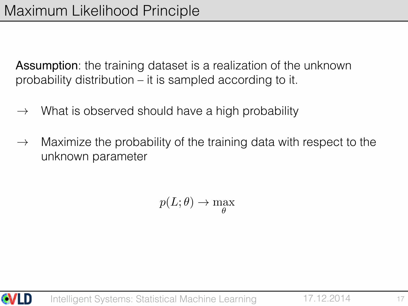
Assumption: the training dataset is a realization of the unknown probability distribution – it is sampled according to it.
What is observed should have a high probability
Maximize the probability of the training data with respect to the unknown parameter
17
Maximum Likelihood Principle
p(L; ✓) ! max
✓
!
!
17.12.2014Intelligent Systems: Statistical Machine Learning
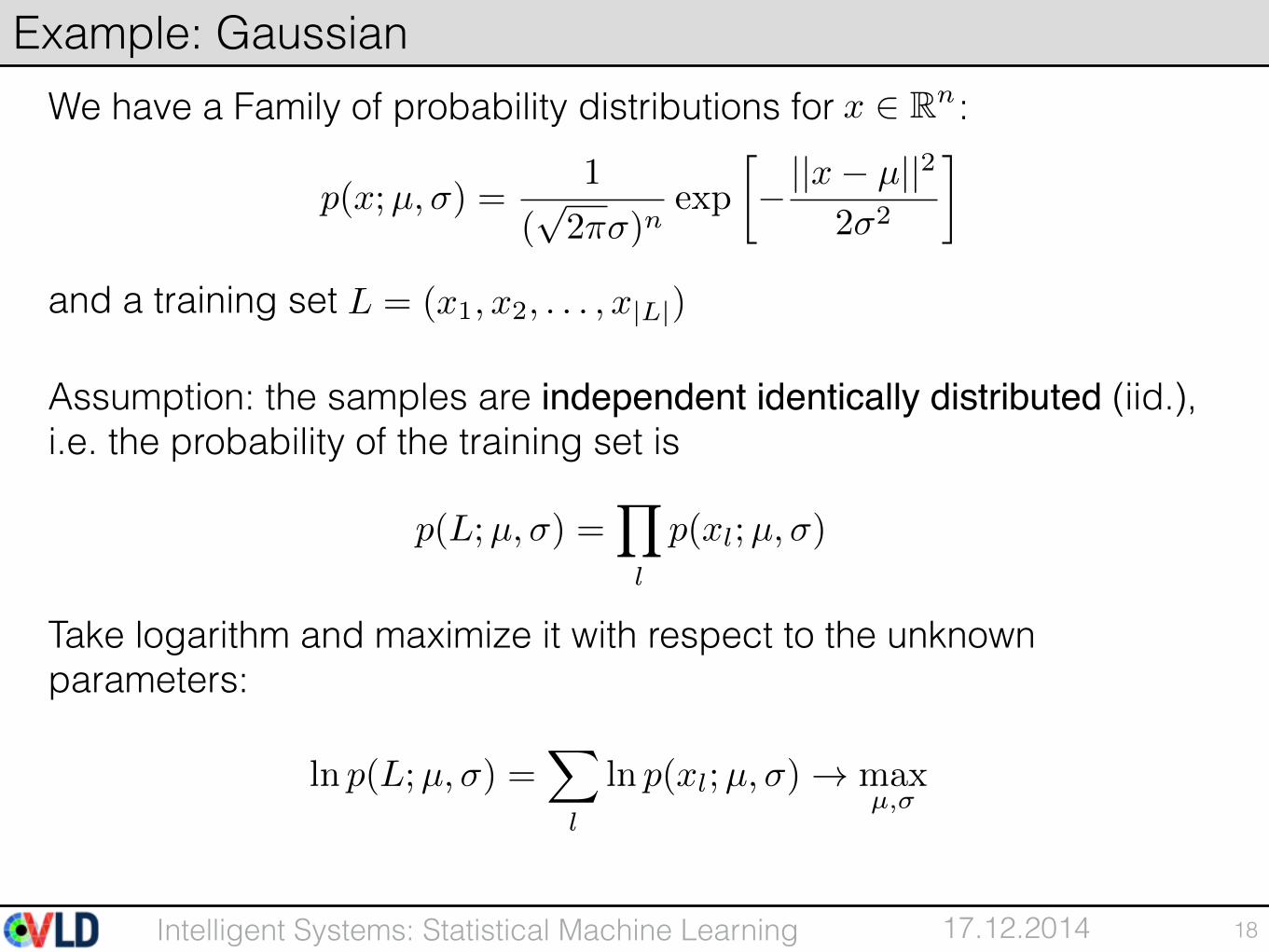
We have a Family of probability distributions for :
and a training set
Assumption: the samples are independent identically distributed (iid.), i.e. the probability of the training set is
Take logarithm and maximize it with respect to the unknown parameters:
18
Example: Gaussian
p(x;µ,�) =
1
(
p2⇡�)
nexp
� ||x� µ||2
2�
2
�x 2 Rn
p(L;µ,�) =Y
l
p(xl;µ,�)
ln p(L;µ,�) =
X
l
ln p(xl;µ,�) ! max
µ,�
L = (x1, x2, . . . , x|L|)
17.12.2014Intelligent Systems: Statistical Machine Learning
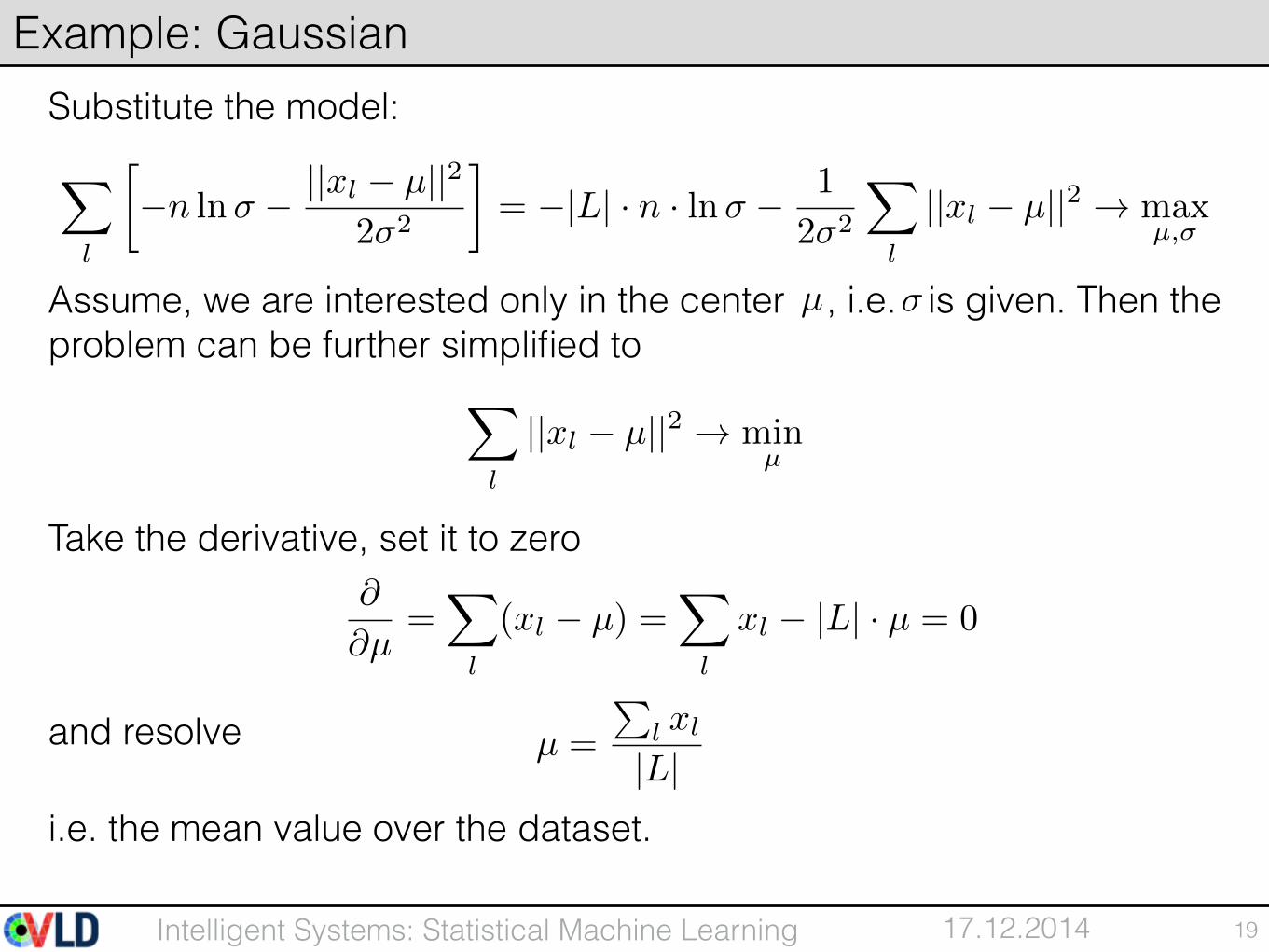
Substitute the model:
Assume, we are interested only in the center , i.e. is given. Then the problem can be further simplified to
Take the derivative, set it to zero
and resolve
i.e. the mean value over the dataset.
19
Example: Gaussian
X
l
�n ln� � ||xl � µ||2
2�
2
�= �|L| · n · ln� � 1
2�
2
X
l
||xl � µ||2 ! max
µ,�
µ �
@
@µ
=X
l
(xl � µ) =X
l
xl � |L| · µ = 0
µ =
Pl xl
|L|
X
l
||xl � µ||2 ! minµ
17.12.2014Intelligent Systems: Statistical Machine Learning
Maximum Likelihood estimator is not the only estimator – there are many others as well.
Maximum Likelihood is consistent, i.e. it gives the true parameters for infinite training sets.
Consider the following experiment for an estimator: 1. We generate infinite numbers of training sets each one being finite; 2. For each training set we estimate the parameter; 3. We average all estimated values.
If the average is the true parameter, the estimator is called unbiased.
Maximum Likelihood is not always unbiased – it depends on the parameter to be estimated. Examples – mean for a Gaussian is unbiased, standard deviation – not.
20
Some comments
17.12.2014Intelligent Systems: Statistical Machine Learning
Today: statistical Machine Learning
• Decision making — Bayesian and non-Bayesian formulations
• Learning — Maximum Likelihood Principle
Next two lectures: models — directed and undirected graphical models
Then: discriminative decision making and learning — neural networks
Then: unsupervised learning — clustering
21
Summary
Top Related