


Languages
Pages
Legal

Institut de la finance structurée et des instruments dérivés de Montréal Montreal Institute of Structured Finance and Derivatives
L’Institut bénéficie du soutien financier de l’Autorité des marchés financiers ainsi que du ministère des Finances du Québec
Document de recherche
DR 15-03
FINANCIAL OLIGOPOLIES: THEORY AND EMPIRICAL EVIDENCE
IN THE CREDIT DEFAULT SWAP MARKETS
Mai 2015
Ce document de recherche a été rédigé par :
Lawrence Kryzanowski Concordia University Stylianos Perrakis Concordia University Rui Zhon Chinese Academy of Finance and Development
L'Institut de la finance structurée et des instruments dérivés de Montréal n'assume aucune responsabilité liée aux propos tenus et aux opinions exprimées dans ses publications, qui n'engagent que leurs auteurs. De plus, l'Institut ne peut, en aucun cas être tenu responsable des conséquences dommageables ou financières de toute exploitation de l'information diffusée dans ses publications.
FINANCIAL OLIGOPOLIES: THEORY AND EMPIRICAL EVIDENCE
IN THE CREDIT DEFAULT SWAP MARKETS
Lawrence Kryzanowski Stylianos Perrakis
Rui Zhong*,†
Abstract
On the basis of the documented oligopolistic structure of the CDS and Loan CDS markets, we
formulate a Cournot-type oligopoly market equilibrium model on the dealer side in both markets. We also
identify significantly positive and persistent earnings from a simulated portfolio of a very large number of
matured contracts in the two markets with otherwise identical characteristics, which are robust in the
presence of trading costs. The oligopoly model predicts that such profitable portfolios are consistent with
the oligopoly equilibrium solution and cannot be explained by alternative absence or limits of arbitrage
theories.
Keywords: Credit Default Swap, Loan Credit Default Swap, Market Efficiency, Market Segmentation, Market Power
JEL Classification: G3, G14, G18, G32
* We thank Jennie Bai, Sean Cleary, George Constantinides, Jorge Cruz Lopez, Jan Ericsson, Louis Gagnon, Genevieve Gauthier, Nikolay Gospodinov, Bing Han, Zhiguo He, Jing-Zhi Huang, Sergey Isaenko, Robert Jarrow, Arben Kita, Chayawat Orthanalai, Wulin Suo, Lorne Switzer, Nancy Ursel, Sarah Wang, Jun Yang, Zhaodong Zhong and participants at the 23rd Annual Derivatives Securities and Risk Management Conference jointly organized by FDIC, Cornell and the University of Houston, the 20th Annual Multinational Finance Society Conference, the 2013 Northern Finance Association Conference, the 2013 Financial Management Association Conference, Frontiers of Finance 2014, China International Conference in Finance 2014, 3rd International Conference on Futures and Derivative Markets and seminars at Queen’s University, University of Windsor, Bank of Canada, Central University of Finance and Economics and Concordia University for helpful comments. Financial support from the Senior Concordia University Research Chair in Finance, RBC Distinguished Professorship of Financial Derivatives, IFSID, and SSHRC (Social Sciences and Humanities Research Council of Canada) are gratefully acknowledged. † Lawrence Kryzanowski and Stylianos Perrakis are with the John Molson School of Business at Concordia University, 1455 De Maisonneuve Blvd West, Montreal, Quebec, Canada H3G 1M8. Rui Zhong is with the Chinese Academy of Finance and Development at Central University of Finance and Economics, 39 College Road, Haidian District, Beijing, China, 100081.
1
FINANCIAL OLIGOPOLIES: THEORY AND EMPIRICAL EVIDENCE IN THE
CREDIT DEFAULT SWAP MARKETS
1. INTRODUCTION
Credit Default Swaps (CDS) and Loan CDS (LCDS) contracts are essentially financial agreements
between protection buyers and protection sellers to transfer the credit risk of the underlying assets
(respectively, corporate debts and syndicated secured loans). The more recent LCDS market has grown
quickly since the introduction of the ABX index in 2006, fueled by the rapid growth in its underlying
asset markets. Compared to traditional CDS contracts, LCDS contracts have higher recovery rates and
cancellability options. Unlike the CDS market, the LCDS market has not been studied as extensively in
the financial literature.
In this paper we formulate a Cournot-style oligopoly model of simultaneous trading in the CDS and
LCDS markets, motivated by recent evidence of the highly concentrated nature of such markets. We also
document positive and persistent profits from portfolios taking opposite positions in two different CDS
contracts on the same reference entity. These profits are confirmed ex post with a very large sample of
matured contracts. Our oligopoly model predicts that the observed profitable portfolios arise as a
consequence of the oligopolistic equilibrium and will persist as long as there are barriers to entry in the
two markets. We extend the model to include trading costs and show that such costs are barriers to small-
scale entry that can be overcome by the traders’ increasing start-up capital as a form of economies of
scale. We show that the profitable portfolios disappear only when the number of oligopolists tends to
infinity, consistent with competitive equilibrium. We use a novel data set and examine empirically the
contrasting predictions of the oligopoly models with the competing limits to arbitrage theory and show
that the evidence overwhelmingly favors the former. To our knowledge, this is the first empirical paper to
apply industrial organization (IO) modeling principles to the study of financial derivatives markets.
The competitive equilibrium limit of our oligopoly also is found to correspond to the same pricing-
parity relation as the no arbitrage equilibrium model. This relation between CDS and non-cancellable
1
LCDS contracts written on the same firm with the same maturity and restructure clauses also involves the
recovery rate estimates for both types of contracts contained in our data set.
1 It assumes no uncertainty of these recovery rate estimates in the event of default but is otherwise
model-free. Using single name CDS and LCDS daily observations on 1-, 3- and 5-year contracts during
the period from April 2008 to March 2012 from datasets provided by the Markit company, we document
time-varying and significantly positive current payoffs on a simulated portfolio that exploits the observed
pricing-parity deviations by simultaneously taking the appropriate positions in the corresponding
markets.2 For the observed CDS and LCDS spreads and the reported recovery rates in the case of default
for both types of contracts,3 the current payoffs to these portfolios are persistently positive over most of
our time series data even after including a generous allowance for transaction costs.4
We apply our portfolios designed to exploit the pricing parity deviations to the subsample of one- and
three-year maturity contracts that have expired within our data period. There were more than 18,000 such
CDS-LCDS contract pairs with pricing parity deviations within the period April 2010-March 2011, after
the financial crisis, in our data set. All of them showed positive cash flows even after a generous
allowance for transaction costs, with an average size that is far too large to be justifiable by counterparty
risk, which anyhow did not materialize anywhere ex post. With such a large sample there is also a
virtually zero probability that the payoffs for longer maturities are rewards for risk due to the unreliability
of the recovery rates reported in the databases as estimates of the “true” recovery rates upon default, given
that the same portfolio selection rules were used in all cases. If our simulated strategies had actually been
applied to these matured contracts at the average notional contract size of $5 million they would have
generated total profits of more than $6.9 billion dollars in total. Thus, although the portfolio payoffs are
1 See Dobranszky (2008) and Ong, Li and Lu (2012) for the discussion of CDS and non-cancellable LCDS parity. 2 The current pricing-parity deviation should be zero under the no arbitrage and no recovery rate uncertainty assumptions. Deviations from parity imply that we observe positive current payoffs on the simulated portfolio. 3 We also call them “Estimated Recovery Rates” since these recovery rates are estimated and provided to Markit by its clients who are active participants in these markets and generally are large financial institutions. 4 Note that this anomaly is emphatically not related to the financial crisis, since it appears throughout the entire period of our data, unlike the violations of arbitrage relations between the CDS and underlying bond markets documented by Alexopoulou, Andersson and Georgescu (2009) and Bai and Collin-Dufresne (2013).
2

not arbitrage profits in the strict sense of the word due to the recovery rate uncertainty and margin
requirements, they correspond to arbitrage in the statistical sense, since the probability of loss is
statistically insignificant.
Motivated by the fact that the number of traders providing quotes in both markets at any point in time
in our data set is small, and by several recent studies documenting the highly concentrated nature of the
CDS markets, we develop an oligopoly model of simultaneous trading in the CDS and LCDS markets.
We consider three different types of agents, those who trade exclusively in only one of the two markets,
CDS and LCDS, and a third type, dealers or arbitrageurs, who trade in both. We show that in such a
setting pricing parity would not hold in equilibrium. In fact, the parity relation requires a perfectly
competitive dealer market for both contracts, while in imperfectly competitive markets it is modified by
the two individual markets’ elasticity ratios. We also show that oligopolists act as arbitrageurs by taking
opposite positions in the two markets. We extend the model to allow for trading costs and different prices
for long and short positions in both markets and show that the conclusions of the frictionless market hold
in a modified form that includes a no trading zone. In fact, trading costs act as a barrier to entry of “small”
firms and the oligopoly becomes a case of competition among the big and the small, as in recent IO
studies.5
In our empirical work, using the number of traders providing quotes in the two markets as a proxy for
the relative level of competition, we find trading profits consistent with this elasticity-modified parity
ratio. We also test formally the market power hypothesis against the alternative of limits to arbitrage
theory. In the former case the observed parity violations are normal outcomes of oligopolistic market
equilibrium, while in the latter they are anomalous and will tend to disappear. In our tests we find no
evidence of long run convergence towards the parity relation to justify the slow moving capital conjecture
as an impediment to arbitrage. In fact, the market seems to react to the absence, rather than the presence
of parity violations, as predicted by our oligopoly model. Most importantly, the duration of the observed
profits in any given pair of CDS-LCDS contracts is strongly positively associated with the size of the
5 See, for instance, Shimomura and Thisse (2012).
2

profits, consistent with a non-competitive market structure and exactly the opposite of what would be
expected under limits to arbitrage. We conclude that market structure is the most likely explanation for
this apparent trading anomaly.6
To our knowledge, this paper is the first to document such anomalous portfolios within credit
derivative markets and to link them specifically to the markets’ non-competitive structure.7 Our paper
contributes to the growing literature on integrated studies of stock, bond, option and CDS markets and to
the more recent studies of the interaction between corporate finance and industrial organization. Earlier
studies have focused on information flows between the various markets but have not uncovered any
tradable anomalies that do not involve privileged information.8 Our results, based on one of the most
popular data sources for credit derivatives, also raise questions on the appropriateness of deriving
financial asset prices based on frictionless competitive equilibrium among different markets without
examining whether the competitive nature of these markets is, in fact, supported by the data.
The consequences of our oligopolistic market structure model are relatively easy to study empirically
in our case because if both CDS and LCDS contracts are written on the same firm the claims are triggered
by the same default events which are defined by the International Swap and Derivatives Association
(ISDA). Thus, the default and survival probabilities of these credit derivatives should be exactly the same
given the same maturities, restructuring clauses and denominated currencies. However, the syndicated
secured loans, the underlying assets of the LCDS, generally have higher priority during the bankruptcy
process compared to senior unsecured debts which are the underlying assets of CDS. The derived market
equilibrium condition implies absence of profitable portfolios only under competitive conditions in the
6 A third possibility suggested by some discussants in earlier versions of this paper, is that the Markit data is not representative of actual trading conditions. Such an explanation would nullify just about every empirical CDS study (many of which have been published in top tier journals), since most of them have used the same data. Further, the Markit data is based on quotes, implying that it at least represents potential trades, which is all that is needed for an arbitrage. 7 Ong, Li and Liu (2012, p. 68) mention that the CDS and LCDS operate on “decidedly inconsistent markets” and present the pricing parity relation developed in the next section, but do not provide any evidence in support of their statement. Atkeson et al (2013) and Bolton and Oehmke (2013) focus on the market structure of credit derivatives but do not use any data in support of their arguments. 8 See, for example, Acharya and Johnson (2007) on insider trading in the CDS and stock markets, Berndt and Ostrovnaya (2008) on information revelation in option, CDS and equity markets, and similar information flow studies by Norden and Weber (2009) and Forte and Pena (2009).
3

dealer market, which are not supported by our data and are anyhow contradicted by recent studies
documenting the highly concentrated nature of the CDS markets. We also verify independently the
regulatory framework and entry conditions in CDS markets and document barriers to entry imposed by
trading platforms on important traders that could have eliminated the profitable portfolios, and examine
the role of margins in preventing small-scale entry.
We verify several other possible explanatory factors that support the alternative limits to arbitrage
theory such as transaction costs, uncertainty of recovery rates, margins, contract illiquidity, slow moving
capital or counterparty risk. In our robustness checks and online appendix we also examine the reliability
of the Markit recovery rate data used in establishing the simulated portfolios, even though this is not a
factor for the observed matured contract payoffs. We find that these data are in almost all cases unbiased
estimates of the realized recovery rates reported in earlier studies and in Moody’s database. We also
confirm that our results are robust to recovery-rate concerns when we estimate the risk-adjusted default
probabilities from the Leland and Toft (1996) structural model estimated using Generalized Method of
Moments (GMM) and data from accounting reports and the equity and option markets. Our results are
also robust with respect to the illiquidity concern, which is a key component of the oligopoly model. In
our online appendix we document fewer positive deviations for the less liquid CDS and LCDS contracts
with maturities other than five years and we show that an illiquidity factor cannot be extracted from a
principal components analysis of the portfolio payoffs.
In the absence of detailed microstructure data that identifies the traders in both markets it is impossible
to confirm with certainty that the observed payoffs of our arbitrage strategy are due to the non-
competitive market structure. The motivation for our theoretical model of oligopoly on the dealer side
arises from the fact that in our data a very small number of traders participate in the CDS and (especially)
the LCDS markets and from several recent studies9 that document a very concentrated market structure in
all CDS markets. In those markets a small number of very large financial institutions act as dealers, while
9 See Atkeson, Eisfeldt and Weill (2013, pp. 7-8), Peltonen, Scheicher and Vuillemey (2014) and Duffie, Scheicher and Vuillemey (2015). .
4
middle-sized and small banks use CDS to hedge their credit exposures.10 More formally, the stylized
general equilibrium model of the banking sector in the NBER study by Atkeson et al (2013) shows that
the market concentration on the CDS dealer side arises under free entry equilibrium due to the differing
sizes of the firms in the banking sector even in the absence of entry deterrence conduct. Thus the barriers
to entry in the dealer market in the CDS-LCDS market pair may be due to economies of scale, again a
well-known phenomenon in the IO literature.11 In commenting on that study, Bolton and Oehmke (2013,
p. 4) point out the possibility of collusion with such high concentration and cite anecdotal evidence of
highly lucrative trading in that market. Further, Peltonen et al (2014) present data according to which in
2011 the 10 largest traders had a market share in excess of 70% in all CDS trading subnetworks. Last,
market power evidence comes from an ongoing antitrust investigation of 13 major US and international
financial institutions by the European Commission for anticompetitive agreements in the CDS markets,
and from the many class action suits filed in the United States. 12 Our oligopoly model shows that
collusion is not required in order to produce profits from intermarket arbitrage and suggests that the
strategies identified in this paper may have already been realized by dealers executing them on their
behalf to the available depth of counterparty traders. We discuss the regulatory implications of our
findings in the last section of this paper.
Our study is not the first one to document absence of integration between markets for related financial
instruments. In fact, the limits to arbitrage approach, introduced by the classic work of Shleifer and
Vishny (1997), has spawned a significant volume of follow up literature, some of which is empirical and
10 Market power on the dealer side in the CDS market has also been documented by Gunduz, Nasev and Trapp (2013), who use microstructure data that identifies traders by type, and by Gupta and Sundaram (2013), who study CDS settlement auctions. 11 This was first pointed out by Bain (1956). See also Perrakis and Warskett (1986). 12 See the July 1, 2013 press statement of the Commission’s Vice-President responsible for competition policy, available at http://europa.eu/rapid/press-release_SPEECH-13-593_en.htm. The first class action suit filed by the Sheet Metal Workers Local 33 Cleveland District Pension Plan against 12 financial institutions and two other entities “seeks “buy side” damages incurred in buying or selling CDS contracts to the “sell side” defendant dealers between 2008 and 2011, alleging that the defendants illegally coordinated to limit competition raising fund managers’ costs” (http://www.ipvancouverblog.com/2013/05/class-action-filed-in-credit-default-swap-cds-case/). During October 2013, The US Judicial Panel on Multidistrict Litigation decided to centralize the cases alleging price-fixing in the market for credit default swaps for the purposes of pretrial proceedings in the District of New Jersey.
5

supportive of the theory.13 In most of this literature, however, the arbitrage relations are model-based and
their failure may be due to model error. What makes our setup unique is the simplicity of the integration
relationship and a model-free parity relation under various market structures, which is clearly not
supported by the data in its competitive no arbitrage format, and the unequivocal confirmation of the ex
post profits from the large sample of matured contracts. Our study is also the first to attribute and
empirically support the lack of integration of the two instruments to imperfect competition.14
The rest of the paper is organized as follows. In Section 2 we briefly describe the CDS and LCDS
markets, including the regulatory environment over the period of the study and the possible barriers to
entry, and present the data and the method of sample selection for the empirical work. Section 3 develops
the simultaneous equilibrium oligopoly market model with and without trading costs. In Section 4 we
present the alternative no arbitrage equilibrium parity relation, which coincides with perfect competition
in our oligopoly model, and construct the simulated portfolio strategy to exploit its violations. Section 5
contains our main empirical evidence in support of the oligopoly model, in the form of a large observed
sample of simulated portfolios with current payoffs (pricing-parity deviations) given transaction costs.
We also discuss other possible reasons apart from oligopoly for the positive payoffs; namely, reward for
risk and limits to arbitrage, and find no support that the payoffs are a reward for bearing risk. Section 6
presents further direct tests of the competing oligopoly market hypothesis over the alternative limits to
arbitrage. Section 7 presents empirical evidence as robustness checks for other limits-to-arbitrage such as
recovery-rate uncertainty, counterparty risk, contract illiquidity and convergence to parity. Section 8
concludes.
13See Deville and Riva (2007), Brav, Heaton and Li (2010), Gârleanu and Pedersen (2011), Lam and Wei (2011), Kapadia and Pu (2012), Bhanot and Guo (2012), Mitchell and Pulvino (2012), Acharya et al (2013), and Hanson and Sunderam (2014). We found few empirical studies of limits to arbitrage in economic journals, although there is awareness of the concept in several theoretical studies; see Stein (2005), Thompson (2010), and Lee and Mas (2012). One such empirical study finds that funds experiencing withdrawals trade in a manner that exacerbates mispricing and that mispricing can persist for months (Mitchell, Pedersen, and Pulvino, 2007). 14 In fact the empirical literature on anticompetitive behavior in financial markets is rather limited and almost exclusively concentrated on stock trading; see the comments in Allen et al (2006, p. 646). The market segmentation in the Canadian option markets documented in Khoury, Perrakis and Savor (2011) was due to an exchange-mandated monopoly at the specialist level.
6
2. CDS AND LCDS MARKETS
2.1 CDS and LCDS Market Overview
The CDS market has existed for a long time but the LCDS market is relatively new and was launched
in 2006 in both the US and Europe.15 It has grown very quickly since its inception because of the rapid
growth in the underlying asset, itself driven by a surge in leveraged buy-outs, and also because of the
introduction of industry-wide documentation published by the International Derivative and Swap
Association (ISDA) to standardize and regulate the LCDS contract. While the reference obligations of
CDS contracts are usually corporate debts, the reference obligations of LCDS contracts are syndicated
secured loans. The LCDS contracts can be divided into Cancellable LCDS (European LCDS) and non-
cancellable LCDS (US LCDS) contracts.16 In this study we concentrate on the US LCDS contract, which
is designed as a trading product that can be used to generate marginal profits by creating a synthetic credit
position where one commits to make (receive) payment in the case of default.17
Similar to an ordinary swap contract, there are physical and cash settlements for both CDS and LCDS
contracts once the settlement is triggered by a credit event. The default settlement mechanism for
European and US LCDS is physical settlement under which the protection seller pays an amount equal to
the notional amount of the reference obligation covered by the LCDS multiplied by the reference price
which is usually 100%.18 Under cash settlement, there is no delivery of the reference obligation and the
protection seller only pays to the protection buyer the difference between par value and the market price
after a credit event. Especially after the financial crisis, cash settlement has become more popular because
the physical delivery of a loan is cumbersome and time consuming. In the cash settlement of a LCDS
contract, the final price of the underlying syndicated loan is determined by an auction methodology.19
15 See Merrill Lynch (2007) and Bartlam and Artmann (2006). The template forms of LCDS documentation were published by International Derivative and Swap Association (ISDA) for the US and European LCDS market on 8th, June 2006 and 2nd, May 2006, respectively. 16 See Shek, Shunichiro and Zhen (2007) and Liang and Zhou (2010) for the valuation of cancellable LCDS. 17 Minton, Stulz and Williamson (2009) find that the use of credit derivatives by US banks is very limited and most of the credit derivatives are held for dealer activities rather than for the hedging of loans. 18 See Bartlam and Artmann (2006), page 5. 19 See the link: http://www.creditfixings.com/CreditEventAuctions/fixings.jsp for the details of CDS Auctions.
7
Short selling constraints are always a major concern when executing trading strategies for traditional
investment instruments, especially for parallel trading in the corporate bond market. CDS and LCDS are
essentially swap agreements between two counterparties to transfer the exposure to the default risk of the
underlying asset. Thus, there is no requirement to hold the underlying assets,20 especially under cash
settlement, which makes an arbitrage position feasible. 21 In the following analysis, we assume cash
settlement for both CDS and LCDS contracts.
2.2 Regulation and Barriers to Entry
Since our data covers totally the financial crisis and partially overlaps with the ongoing regulatory
reform of the Dodd-Frank Act, our empirical results took place under differing regulatory regimes. Over
the period examined herein, CDS contracts have become more standardized, and electronic processing
and central clearing of trades have increased but bilateral trades have apparently continued throughout the
entire period. Regulatory approvals by the Securities and Exchanges Commission (SEC) dealing with
margin requirements include an interim pilot program for dealer members of the Financial Industry
Regulatory Authority (FINRA) in 2009 (Rule 4240) which was further extended, for example, in 2011.To
increase transparency and reduce systemic risk, a central clearing corporation (CCP) was introduced by
several trading platforms during the period to clear standard contracts. The first was the Intercontinental
Exchange (ICE) in March 2009.
Under central clearing there is an intermediary between long and short positions that reduces
counterparty risk by guaranteeing the execution of the swap agreements by monitoring the positions and
market exposure of each clearing member to ensure that sufficient funds are on deposit to cover each
member’s risks. Institutions wishing to participate as dealers on the CCP can become CCP members
provided that they have an A credit rating and a net worth of at least $5 billion. In other words, there are
clear scale effects in potential entry into the dealer function, especially given the fact that the A credit
rating would rule out most hedge funds. Note that the evidence presented in the NBER study by Atkeson
20 This is the so-called “naked” or “synthetic” contract. 21 See Mengle (2007).
8

et al (2013, Figure 2) shows that as of the end of 2011 only 12 of the largest bank holding companies
trading in derivatives had trading assets in excess of that amount.
These entry restrictions are probably responsible for the undeniable fact of high concentration in the
CDS market, let alone the dealer function, documented in several studies. Thus, in addition to the
aforementioned NBER study a recent paper notes that in 2011 the 10 largest traders had a market share in
excess of 70% in all CDS trading subnetworks. The authors also state (p. 119) that the CDS market “…is
highly concentrated around 14 dealers, who are the only members of central counterparties…”. 22
Concerning the role of margins as barriers to entry, we note that traders are allowed to net out their
margin positions, with the result that in 2011 the collateral to gross notional ratio in CDS trades was
0.78%, far below the ICE margins.23 This netting out tends to favor large market participants who can
hold multiple positions and who also enjoy the benefits of greater holding diversification. In our
robustness checks we examine the role of margins for the matured one-year contracts using the ICE
margins under the most adverse conditions.
In conclusion, therefore, the evidence on the institutional environment faced by those willing to trade
in the CDS-LCDS market pair is that, although there are no formal regulatory barriers, there is high
concentration of trading and serious restrictions to entry into the dealer function in both markets. This, in
turn, motivates our oligopoly model to study intermarket arbitrage.
2.3 Sample and Data for the Empirical Work
For the empirical part of this paper we obtain our CDS and LCDS data from Markit who collects the
quotes on LCDS spreads from large financial institutions and other high quality data sources and
produces the LCDS spread database on a daily basis starting from April 11, 2008. Our sample is from
April 11th, 2008 to March 30th, 2012, which encompasses the credit crisis and the accompanying
recession. We only use US (non-cancellable) LCDS to construct the portfolios. As a robustness check on
22 See Peltonen, Scheicher and Vuillemey (2014, p. 119). 23 See Duffie, Scheicher and Vuillemey (2015).
9
the size of the transaction costs, we also match part of our CDS sample to intraday quote data also
provided by Markit in a separate data base.
In the CDS market we select the contracts on senior unsecured debts since this type of contract is the
most liquid and is used frequently in the literature. In the LCDS market, we select the contracts on the
first-lien syndicated loans since the claims on collateral for the first-lien loans are senior to those of the
second-lien loans, which indicate more reliable estimated recovery rates for these loans. In addition, the
LCDS contracts on first-lien loans form the majority in our data source and are more liquid than those on
the second-lien loans. We restrict our CDS and LCDS contracts to those in the United States and
denominated in US dollars. To ensure that the first-passage default and survival probabilities of the CDS
contracts are exactly the same as those of the corresponding LCDS, we match the daily LCDS and CDS
data based on company name, denominated currency, restructure clauses and time to maturity. We focus
on the contracts with a 5-year maturity since they are the most liquid contracts and the most studied in the
previous literature.24 We also study in some detail the 1-year and 3-year maturities, since they contain
many matured contracts within our data set. The contracts with 7-year and 10-year maturities are studied
as robustness checks.
A key component of any CDS market model is the recovery rate upon default. To proxy for the
unobservable real recovery rates we use the estimated recovery rates extracted from our Markit datasets,
which are based on the raw data providers’ estimates.25 These recovery rate expectations at time of issue
may differ from subsequent recovery-rate expectations and actual recovery rates.26 Nevertheless, these
Markit estimates represent the only available proxy for the real recovery rates27 and have been used
repeatedly in previous studies.28
24 See Jorion and Zhang (2009), Cao, Yu and Zhong (2010, 2011), Schweikhard and Tsesmelidakis (2012), Qiu and Yu (2012) and Zhang, Zhou and Zhu (2009). 25 Based on Markit CDS and Bonds User Guide, their clients can also contribute their recovery rates. Data on recovery rates are denoted throughout the Markit product as Client Recovery. 26 Jokivuolle and Peura (2003), Altman, Brady, Resti and Sironi (2005), Hu and Perraudin (2002) and Chava, Stefanescu and Turnbull (2006) report that the recovery and default rates are negatively correlated. 27 The real recovery rates are collected from Moody’s Default and Recovery Database and discussed in Section 4. 28 See Huang and Zhu (2008), Zhang, Zhou and Zhu (2008), and Elkamhi, Ericsson and Jiang (2012). Loon and Zhong (2014, pp. 112-113) give a detailed description of the Markit data collection procedures.
10
2.4 Data Description
[Insert Table 1 about here]
Table 1 reports the summary statistics for our full sample and the sub-samples classified by credit
rating. We eliminate the observations whose CDS spreads (or LCDS spreads) are greater than 1 and the
single name contracts which have less than 120 consecutive daily observations. In addition, we obtain the
accounting variables from COMPUSTAT, economic macro variables from Federal Reserve H.15
database and equity trading information from CRSP. After merging all these datasets and removing the
missing observations and private firms, the full sample contains 68,147 firm-clause-daily cross-sectional
observations for 120 single names during the sample period from April 11, 2008 to March 30, 2012.
In the full sample, the mean LCDS and CDS spreads are around 3.7% and 4.6%, respectively. Both
medians are smaller than their corresponding means which indicate asymmetric distributions and fat tails,
especially on the right side. These style factors are also verified by positive skewness for the CDS and
LCDS spreads. The distributions of recovery rates estimates for the LCDS and CDS contracts are close to
a Gaussian distribution with slightly negative skewness. Both the mean and median of the LCDS recovery
rates, around 65% and 70% respectively, are greater than the corresponding statistics for the CDS
contracts, around 38% and 40% respectively. The syndicated secured loans (the underlying assets of
LCDS) are usually backed up with collateral and have claim priority compared to the senior unsecured
debts which are the underlying assets that back the CDS once the default event occurs.29 The sub-sample
of investment grades (includes firms rated greater than or equal to BBB), accounts for more than 60% of
the total observations, while junk-rated contracts and not rated contracts share almost equally the rest of
the observations, approximately 20% each. As expected, both the mean and median of the CDS and
LCDS spreads in the investment grade sub-sample are relatively lower compared to the junk and not rated
sub-samples, while the mean and median of the recovery rates are broadly similar in all three sub-
samples. There are also differences in the accounting variables among the sub-samples, with the junk
29 This implies that the LCDS recovery rate estimates should exceed the corresponding CDS ones. This turns out to be true for all but 265 out of the 68,147 pairs of data points. For more on the priority of the LCDS claims see Section 5.5.
11

firms being smaller and more heavily indebted than the investments grade firms. The not-rated firms are
mostly relatively small firms in terms of their total assets, with diverse accounting ratios.
We observe extremely high first-order autocorrelations in the daily spreads for CDS (around 0.98) and
LCDS (around 0.97) indicating a spread clustering effect in both markets. The first-order autocorrelation
of LCDS recovery rates of approximately 0.93 is much higher than that for CDS recovery rates of around
0.77. This further supports the conjecture that LCDS recovery rates are more persistent and reliable
compared to their counterparts for CDS contracts. If we lower the frequency of the data from daily to
quarterly, the first-order autocorrelations decrease significantly for all the variables.
The daily idiosyncratic volatilities 30 of the full sample have a mean around 2.4% with positive
skewness and extremely high kurtosis. As expected, both the mean and median of daily idiosyncratic
volatilities of the investment grade firms are relatively lower than those of junk-rated firms. For the not
rated firms, the daily idiosyncratic volatilities are more volatile compared to the other sub-samples.
3. AN OLIGOPOLY EQUILIBRIUM MODEL OF CDS AND LCDS MARKETS
3.1 The Structure of the CDS and LCDS Markets: Further Evidence
In most of the financial literature the valuation of CDS and LCDS contracts is normally done by a no
arbitrage methodology and by assuming that the values of the two cash flows involved in a swap are
equal. An additional implicit assumption is that the markets are perfect and competitive. As we discussed
in the previous sections, the available evidence does not support this assumption, which is further
examined in this subsection on the basis of our dataset.
We assess the imperfectly competitive structure of both markets from the number of distinct dealers
providing daily quotes on the 5-year CDS and LCDS contracts as reported in the Markit data base.31 In
the full sample there are on average 5 and 1.6 dealers quoting on the same firm’s CDS and LCDS
30 The calculation details are provided in Section 6. 31 Qiu and Yu (2012) use the same liquidity measure to study the liquidity in the single-name credit default swap market. This is consistent with the theoretical model of Grossman and Miller (1988) that explains the relation between liquidity and the number of market makers given no barriers or stickiness to entry. With regard to entry stickiness, the second critical assumption in the modeling of a run on a financial market by Bernardo and Welch (2004) is that the market making sector is risk-averse in the aggregate and cannot expand infinitely in an instant.
12
contract, respectively, demonstrating the relatively higher dealer participation and liquidity of the CDS
compared to the corresponding LCDS contracts. As the rating decreases from investment to junk grade,
we document a significant decrease of CDS liquidity, from 5.92 to 4.96, and a slight decrease of LCDS
liquidity, from 1.67 to 1.64, on average. In the not rated sub-sample the liquidity of CDS contracts is
reduced even further and all of them have the same average number of dealers, two. On the other hand,
the liquidity of the LCDS contracts moves in the opposite direction, increasing to 1.88 on average, higher
than in the rated contracts.
Our data, therefore, shows a strongly concentrated structure at the dealer level. To see its
consequences we model the simultaneous market equilibrium in both markets assuming initially the
absence of frictions and an oligopoly at the dealer level. Our simplified model abstracts from some
realistic market features but is quite general in its assumptions and retains the necessary elements for the
equilibrium analysis. It also contains the competitive and monopoly structures as limit cases.
3.2 A Frictionless Cournot Oligopoly at the Dealer Level
For every single firm on which CDS and LCDS contracts are traded we distinguish three categories of
agents and two markets denoted by the subscript 1, 2i = for the CDS and LCDS respectively. In each
market ic and iR , 1, 2i = , denote the corresponding premium and recovery rate estimate contained in the
database. Two classes of agents are assumed to trade exclusively in each one of the two markets for
insurance or speculative purposes, who may or may not hold the firm’s bonds and credit lines,
respectively.
We do not model the behavior of these two groups but represent each group’s joint decisions by the
function ( ), 1, 2iD iC c i = , the net demand volume of contracts (long minus short, or the conventional
demand curve minus the conventional supply curve in the corresponding market) in markets 1, 2i = , a
decreasing function that becomes negative for sufficiently high values of the ic ’s indicating net short
positions. For reference purposes we also consider the equilibrium premiums, which equalize the traded
13
volume of contracts for each group of agents, and are denoted by ˆ , 1, 2ic i = . It is assumed that the
demand functions are exogenous, and that the marginal revenues [ ( )] , 1, 2
ii D i
i
d c C c idc
= increase as the
prices increase or the quantities decrease, the usual assumptions for oligopoly equilibrium. The agents’
net positions are negative (positive) whenever i ic c≤ ( i ic c≥ ). 21 R− and 11 R− denote the expected
losses in the LCDS and CDS contracts, respectively, in the event of default. Recognition of the priority
rule implies 2 11 1R R− < − .32
We model explicitly the decisions of the third category of traders in the two markets, the 1J ≥ traders
termed arbitrageurs or dealers, who trade simultaneously in both markets and provide the residual
liquidity to clear the markets. We consider a two-period horizon (0 and 1), with the terminal date
corresponding to the maturity of the contracts. Let , 1, 2iY i = denote the arbitrageurs’ net demand in the
two markets at contract maturity, for which we must have the clearing condition, omitting the time
subscript:
( ) 0, 1, 2iD i iC c Y i+ = = (3.1)
Each arbitrageur 1,..., , [1, ]j J J= ∈ ∞ is assumed to choose her demand jiy , j
i ij
y Y=∑ , 1, 2i =
by maximizing the expected utility of a function 1( )j jU W of discounted terminal wealth 1jW at the
maturity of the contracts. Apart from concavity and decreasing absolute risk aversion (DARA), we do not
impose any other restrictions on the utility functions, nor do we assume that they belong to the same
family. 33 Since the product is homogenous in both markets, in the absence of collusion the joint
32 The recovery rates represent expectations at contract time given default within the contract period, conditional on asset value or possible macroeconomic variables; they need not be assumed constant. In the financial literature’s structural models of the firm the losses given default are non-increasing functions of the unlevered asset value. 33 Several theoretical studies on arbitrage assume that the utilities of all investors belong to the Constant Absolute Risk Aversion (CARA) type, 1exp( )j jWα− ; see for instance Gromb and Vayanos (2002, 2010) and Fardeau (2012, 2014). While such a formulation simplifies the equilibrium expressions, our important results do not need it for their proofs.
14
equilibrium is a Cournot oligopoly, with each arbitrageur choosing jiy by the maximization of expected
utility, withτ denoting the random default time and ( )SP τ , ( )DP τ , the corresponding probabilities of
survival and default within the contract horizonT
1 2
1 2
1,
1 1,0 0
{ [ ( )]}
{ ( ) ( ( ) ) ( ) ( ( ) ) }
1,...,
j j
j j
j jy y
T TS j j D j j
y y
Max E U W
Max P U W S d P U W D d
j J
τ τ τ τ τ τ= +
=
∫ ∫ (3.2)
In this maximization all ,kiy k j≠ are taken as given, , 1, 2j
i ij
y Y i= =∑ , as per the market
equilibrium condition (3.1), and the wealth constraint (3.3) holds, with 0jW denoting the initial wealth34
and with 1 ( )jW τ given by
1 0 1 1 1 2 2 2 1
1 0 1 1 2 2 1
{ [(1 ) ] [(1 ) ]} ( ) , [0, ]
{ } ( ) , (survival) [0, ]
j j r j j j
j j j j r j
W W e y R c y R c W D if default at T
W W y c y c e W S if no default for all T
τ
τ
τ τ
τ τ
−
−
= + − − + − − ≡ ∈
= − + ≡ ∈. (3.3)
To evaluate the expectation in (3.2) the utility of terminal wealth is weighted by the default and
survival probabilities. It is integrated over the entire contract length, representing the discount factors and
the probabilities of default and survival respectively at any time during contract duration.
The maximization of the objective function (3.2) yields the following first order conditions (FOC) for
the joint equilibrium
10
1 10 0
1
(1 ) ( ) '( ( ) )(1 )
( ) '( ( ) ) ( ) '( ( ) )
( ), 1, 2
TD j j
i ji
iT T iS j j D j j i D
jj i
i D i
R P U W D dyc
YP U W S d P U W D d
y C c i
τ τ τ
ετ τ τ τ τ τ
−= +
+
= − =
∫
∫ ∫
∑
(3.4)
34 Since the dealers are assumed, following Shleifer and Vishny (1997), to be “highly specialized investors using other people’s capital”, the initial wealth is a proxy for economies of scale at the dealer level and will be shown to play an important role on entry further in this section. They also represent the capacity to cover required margins.
15
Where 1'( ( ) )j jU W Dτ and 1'( ( ) )j jU W Sτ denote the marginal utilities of the jth arbitrageur under
firm default and survival respectively, and '
'( ) , , 1, 2i i
i ii D DD i Di
D i
c C Cc C iC c
ε ∂= ≡ =
∂ denote the price
elasticity of demand in each market.
Dividing the two relations in (3.4) with each other, we get the following result
11 1
1 1
2 22 2
2
(1 )11(1 )
j
Dj
D
ycY R
y RcY
ε
ε
+−
=−+
(3.5)
Let now
1* * *0
1 10 0
( ) '( ( ) )1( ), ( )
( ) '( ( ) ) ( ) '( ( ) )
TD j
T TjS j D j
P U W D dj j
JP U W S d P U W D d
τ τ τ
τ τ τ τ τ τ≡ Ψ Ψ ≡ Ψ
+
∫∑
∫ ∫ (3.6)
denote, respectively, the common factor in the two equations of (3.4) evaluated at the optimal number of
contracts and its summation over j . Aggregating equations in (3.4) and dividing by J on both sides, we
eliminate the market shares from (3.4) and obtain the equilibrium relations for the average dealer
participating in the two markets:
* 1(1 ) (1 ), 1, 2i i iD
R c iJε
− Ψ = + = . (3.7)
Observe also that relations (3.4) and (3.7), although they are the outcome of a Cournot-style oligopoly
equilibrium, are in fact consistent with the conventional valuation relations of asset pricing theory,
defined in footnote 40 in the following section. Indeed, the left-hand-side (LHS) of both relations is the
expected cost of default in the two markets in the risk neutral world, where the default probabilities have
been weighed by the arbitrageurs’ marginal utilities, individually and as a market aggregate respectively.
These risk-adjusted costs are equated to the individual and aggregate marginal revenues.
Taking the ratio, we get the following result,
16
1 1
1
22 2
1(1 )1
1 1(1 )D
D
cJ R
RcJ
ε
ε
+−
=−+
(3.8)
In line with standard results for the Cournot game, we note that relation (3.8) contains as special cases
both the competitive case for J →∞ , when the elasticity effect disappears, and the monopoly case for
1J = . In the following section we show that the competitive case is a more general version of a valuation
relation under no arbitrage assumptions in the absence of transaction costs. Such a relation emerges as a
special case of the oligopoly equilibrium if the recovery rates are constant under competitive conditions in
the dealer market (infinitely many arbitrageurs and no minimum scale restrictions), where each
arbitrageur maximizes (3.2) with respect to , 1, 2jiy i = , given 1c and 2c . In the absence of competition
each contract premium must be modified by the elasticity and the number of dealers. In other words, if the
observed ratio 1 1
2 2
11
c Rc R
−≠
−, it may be either because there is mispricing or because there is imperfect
competition and market power at the dealer level. In the former case we expect changes over time would
converge to the “correct” ratio (slow moving capital). In the latter case no such convergence is to be
expected, since (3.8) holds and the equilibrium ratio also depends on the demand elasticities and the
number of Cournot dealers. In our model J is common to both markets, since the arbitrageurs provide
liquidity to both markets. Nonetheless, the two-market Cournot equilibrium is entirely consistent with our
data, in which one market (the CDS) has a larger number of traders than the other. Those traders
participating in only one of the two markets are absorbed by the market demand curve.
3.3 Properties of the Frictionless Cournot Equilibrium
An arbitrage between the CDS and LCDS markets is defined as an equilibrium in which 1jy and 2
jy
have different signs in the Cournot equilibrium relations (3.4) for every dealer. The following result,
proven in the appendix, shows that this equilibrium does, indeed, correspond to an arbitrage.
17

Proposition 1: If *1jy and *
2jy denote the optimal quantities for the thj Cournot player then their signs
are opposite and the oligopolist acts as an arbitrageur between the two markets.
Proposition 1 implies that each Cournot player participates in opposite sides in the two markets and
1 2( ) 0j jsign y y < , for all j , or that arbitrage trading is part and parcel of market equilibrium in the
oligopoly structure. Furthermore, such trading is not the result of collusion or otherwise non-competitive
behavior but appears as an optimal strategy in a competitive oligopoly game. This conclusion has certain
empirical implications that are explored in subsequent sections.
The following result can also be shown for the Cournot equilibrium in all cases and for all players.
Proposition 2: If *jiy and *k
iy , 1,2i = denote the optimal contracts for two different Cournot players,
then * *1j k
iy y≥ implies * *2 2j ky y≤ and vice versa.
Proposition 2 implies that, if 1* *1 ... J
iy y≥ ≥ , then 1* *2 2... Jy y≤ ≤ . In other words there is a scale effect,
with a large market share in one market implying also a similarly large market share of an opposite sign
in the other market. Observe that these inequalities do not necessarily imply that all Cournot players adopt
the same arbitrage strategy. Indeed, suppose that 1 0Y > and 2 0Y < . Then appendix relation (A.2)
implies that, if 1* *1 ... J
iy y≥ ≥ we must also have * *(1) ... ( )JΨ ≤ ≤ Ψ , but while necessarily 1*1 0y > and
1*2 0y < , we may still have *
1 0jy < and *2 0jy > beyond some value of *j .
3.4 Cournot Equilibrium Under Trading Costs
Let again ( ), 1, 2iD iC c i = denote the net demand volume of CDS contracts in the frictionless
economy, and , 1, 2ik i = the trading costs. We assume that for any CDS-LCDS contract pair these costs
are platform-wide and exogenously determined, applicable to all such pairs. In other words, our dealer
oligopoly determines jointly the trading costs for the platform, but lets the dealers compete as Cournot
players in each contract pair. By definition, at the competitive frictionless equilibrium premiums
ˆ , 1, 2ic i = we have ˆ( ) 0, 1, 2iD iC c i= = .
18
The demand curves in the presence of trading costs become discontinuous, lowering (raising) the
positive (negative) quantity segment by , 1, 2ik i = . Instead of equation (3.1) we now have
ˆ( ) ( ) 0, ( ) 0 ( <0) for , 1, 2ˆ( ) ( ) 0, ( ) 0 ( 0) for , 1, 2
ˆ ˆ0, [ , ] 1, 2
i i iD i i i D i i D i i i i i i
i i iD i i i D i i D i i i i i
i i i i i i
C c k Y C c Y if C c k Y c c k iC c k Y C c Y if C c Y c c k i
Y if c c k c k i
−
+ +
− + ≡ + = − > < − = + + ≡ + = < > > + = = ∈ − + =
(3.9)
In other words, the dealers provide the counterparty short (long) demand when the premium is
sufficiently low (high), while they refrain from trading for the intermediate premium values.
The objective function, equations (3.2)-(3.3), remains the same, with the difference that now instead of
ic we have i ic k+ and i ic k− , 1, 2 i = , depending on the sign of the corresponding jiy .35 Adopting the
innocuous assumption that all dealers trade in the same direction, it can also be easily shown that
Proposition 1 also holds in the environment with frictions. In such a case we have, instead of (3.4) and
setting + or – as superscript to the elasticity corresponding to the equivalent demand ( )iD iC c+ or ( )i
D iC c− :
For a short position in CDS and long in LCDS we have
* 11 1 1 1
1
* 22 2 2 2
2
1 21 1 2 2
1 1
(1 ) ( ) ( )(1 )
(1 ) ( ) ( )(1 )
( ), ( )
j
Dj
Dj j
j jD D
yR j c kY
yR j c kY
y C c y C c
ε
ε
−
+
− +
− Ψ = − +
− Ψ = + +
= − = −∑ ∑
(3.10a)
Conversely, for a long position in CDS and short in LCDS we have
35 The presence of trading costs raises questions of the existence of an arbitrage equilibrium as we defined in our oligopoly model, in the sense that none of the J dealers may find it profitable to trade in both markets. Since existence depends on the size of the trading costs and the unobservable demands, we assume for empirical purposes that a (3.10a) or (3.10b) equilibrium exists for the J dealers in our markets. See also the following subsection.
19
* 11 1 1 1
1
* 22 2 2 2
2
1 21 1 2 2
1 1
(1 ) ( ) ( )(1 )
(1 ) ( ) ( )(1 )
( ), ( )
j
Dj
Dj j
j jD D
yR j c kY
yR j c kY
y C c y C c
ε
ε
+
−
+ −
− Ψ = + +
− Ψ = − +
= − = −∑ ∑
(3.10b)
Aggregating again over the participating dealers in both markets we observe that the frictionless
equilibrium (3.7) is replaced by the following pair of equations (3.11a)-(3.11b), corresponding,
respectively, to the case where the dealer is short (long) in the CDS (LCDS) and long (short) in the LCDS
(CDS) market.
* *1 1 1 2 2 21 2
1 1(1 ) ( )(1 ), (1 ) ( )(1 ) D D
R c k R c kJ Jε ε− +− Ψ = − + − Ψ = + + (3.11a)
* *1 1 1 2 2 21 2
1 1(1 ) ( )(1 ), (1 ) ( )(1 ) D D
R c k R c kJ Jε ε+ −− Ψ = + + − Ψ = − + (3.11b)
3.5 Entry in the Competitive Cournot Equilibrium under Frictions
In the frictionless market the participating competitive oligopolists are exogenously determined and
entry is theoretically feasible at any scale. As pointed out in previous sections, in practice entry is limited
by economies of scale at the dealer level under the form of fixed entry costs that prevent small financial
institutions from entering.36 Here we show that trading costs as modeled in this section may act as barriers
to entry, and a type of (3.11a) or (3.11b) equilibrium may exist where individual dealers may not find it
profitable to participate in either one or both markets depending on their utility function. We also show
that economies of scale proxied by an increase in the initial endowment 0jW may overcome the trading
cost barriers to small scale entry.
Suppose a type of (3.11a) or (3.11b) Cournot equilibrium exists and consider a “small-scale” entrant
' [1, ]j j J∉ ∈ who considers entry at an infinitesimally small output and acts as a price taker. We then
prove the following in the appendix.
36 See Atkeson et al (2013, p. 11).
20

Proposition 3: Given a type (11a) or (11b) equilibrium, a price-taking entry for entrant ' [1, ]j j J∉ ∈
is not feasible in both markets if the following conditions hold
( ) 11 2 2 1
2
11
Rc c k kR
−< + +
− for a type (11a) equilibrium (3.12a)
( ) 11 2 2 1
2
11
Rc c k kR
−> − −
− for a type (11b) equilibrium (3.12b)
Observe that (3.12a-b) define a no trade zone given the relative prices in the two markets that is
identical to the zone defined in (4.6) and determined by a no arbitrage model in the following section,
with the important difference that the two premiums are values determined by oligopoly, rather than no
arbitrage, equilibria. A testable implication of Proposition 3 is that the number of arbitrageurs decreases if
the transaction costs , 1, 2ik i = rise.
The last theoretical result of this paper refers to the role of economies of scale proxied by the initial
wealth 0jW in overcoming barriers to small-scale entry. 37 In the appendix we prove the following, under
slightly different assumptions.
Proposition 4: Under the DARA property and assuming constant probabilities ( )SP τ and ( )DP τ for
allτ an increase in 0jW may eliminate the barriers to small-scale entry in both the short and the long
markets and for both types of equilibria (3.12a) and (3.12b).
Although Propositions 2-4 do not have empirical implications due to lack of data, they do illustrate the
importance of scale in determining the CDS markets’ competitive structure. All results hold under general
non-competitive conditions and without any restrictions on dealer preferences beyond risk aversion and
the DARA property. Still, they are sufficient to test the market power hypothesis, as we show in the
following section.
37 A full analysis of entry barriers also needs to consider entry that alters the oligopolistic equilibrium as in Atkeson et al (2013). Such an analysis is not feasible without reducing significantly the generality of the modeling of the two-market Cournot equilibrium and lies beyond the objectives of this paper.
21
4. CDS AND LCDS NO ARBITRAGE PARITY
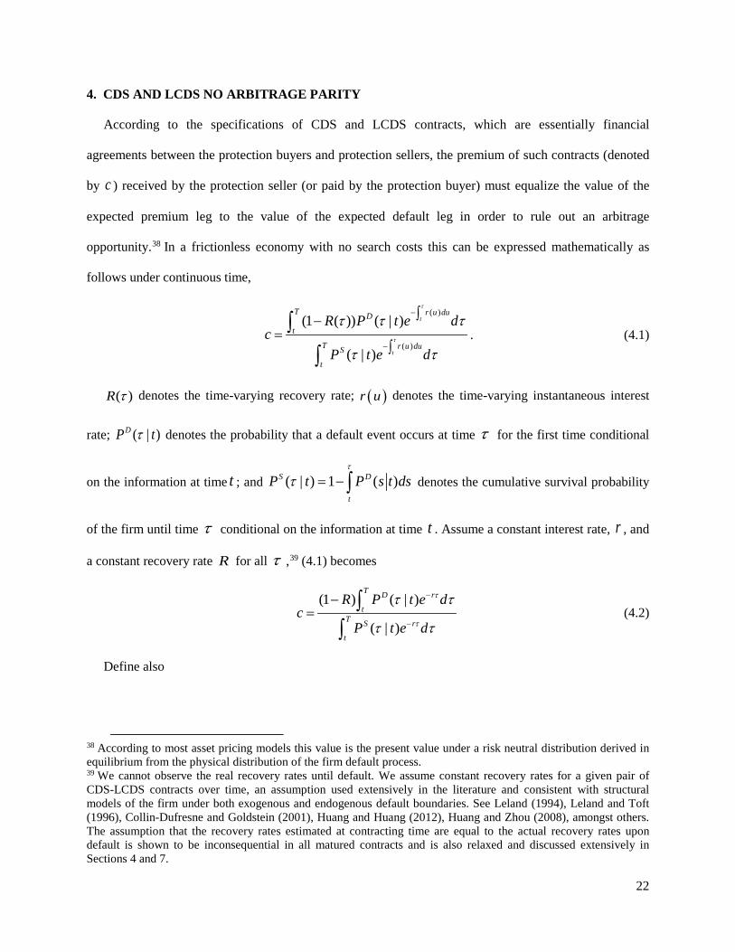
According to the specifications of CDS and LCDS contracts, which are essentially financial
agreements between the protection buyers and protection sellers, the premium of such contracts (denoted
by c ) received by the protection seller (or paid by the protection buyer) must equalize the value of the
expected premium leg to the value of the expected default leg in order to rule out an arbitrage
opportunity.38 In a frictionless economy with no search costs this can be expressed mathematically as
follows under continuous time,
( )
( )
(1 ( )) ( | )
( | )
t
t
T r u duD
t
T r u duS
t
R P t e dc
P t e d
τ
τ
τ τ τ
τ τ
−
−
∫−=
∫∫
∫. (4.1)
( )R τ denotes the time-varying recovery rate; ( )r u denotes the time-varying instantaneous interest
rate; ( | )DP tτ denotes the probability that a default event occurs at time τ for the first time conditional
on the information at time t ; and ( | ) 1 ( )S D
t
P t P s t dsτ
τ = − ∫ denotes the cumulative survival probability
of the firm until time τ conditional on the information at time t . Assume a constant interest rate, r , and
a constant recovery rate R for all τ ,39 (4.1) becomes
(1 ) ( | )
( | )
T D r
tT S r
t
R P t e dc
P t e d
τ
τ
τ τ
τ τ
−
−
−= ∫
∫ (4.2)
Define also
38 According to most asset pricing models this value is the present value under a risk neutral distribution derived in equilibrium from the physical distribution of the firm default process. 39 We cannot observe the real recovery rates until default. We assume constant recovery rates for a given pair of CDS-LCDS contracts over time, an assumption used extensively in the literature and consistent with structural models of the firm under both exogenous and endogenous default boundaries. See Leland (1994), Leland and Toft (1996), Collin-Dufresne and Goldstein (2001), Huang and Huang (2012), Huang and Zhou (2008), amongst others. The assumption that the recovery rates estimated at contracting time are equal to the actual recovery rates upon default is shown to be inconsequential in all matured contracts and is also relaxed and discussed extensively in Sections 4 and 7.
22
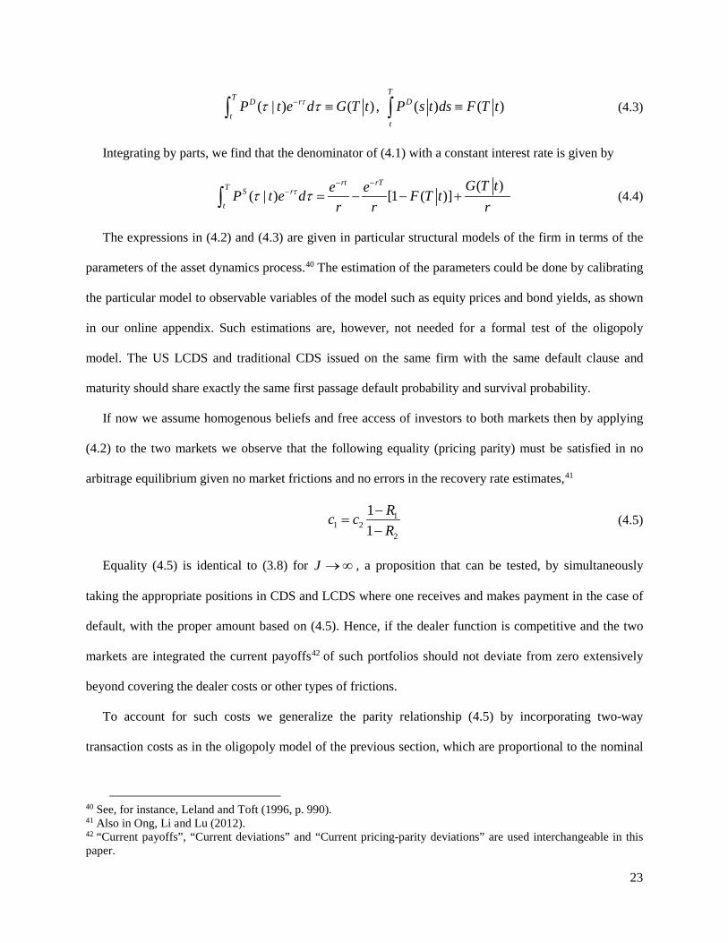
( | ) ( ) , ( ) ( )T
T D r D
tt
P t e d G T t P s t ds F T tττ τ− ≡ ≡∫ ∫ (4.3)
Integrating by parts, we find that the denominator of (4.1) with a constant interest rate is given by
( )
( | ) [1 ( )]rt rTT S r
t
G T te eP t e d F T tr r r
ττ τ− −
− = − − +∫ (4.4)
The expressions in (4.2) and (4.3) are given in particular structural models of the firm in terms of the
parameters of the asset dynamics process.40 The estimation of the parameters could be done by calibrating
the particular model to observable variables of the model such as equity prices and bond yields, as shown
in our online appendix. Such estimations are, however, not needed for a formal test of the oligopoly
model. The US LCDS and traditional CDS issued on the same firm with the same default clause and
maturity should share exactly the same first passage default probability and survival probability.
If now we assume homogenous beliefs and free access of investors to both markets then by applying
(4.2) to the two markets we observe that the following equality (pricing parity) must be satisfied in no
arbitrage equilibrium given no market frictions and no errors in the recovery rate estimates,41
11 2
2
11
Rc cR
−=
− (4.5)
Equality (4.5) is identical to (3.8) for J →∞ , a proposition that can be tested, by simultaneously
taking the appropriate positions in CDS and LCDS where one receives and makes payment in the case of
default, with the proper amount based on (4.5). Hence, if the dealer function is competitive and the two
markets are integrated the current payoffs42 of such portfolios should not deviate from zero extensively
beyond covering the dealer costs or other types of frictions.
To account for such costs we generalize the parity relationship (4.5) by incorporating two-way
transaction costs as in the oligopoly model of the previous section, which are proportional to the nominal
40 See, for instance, Leland and Toft (1996, p. 990). 41 Also in Ong, Li and Lu (2012). 42 “Current payoffs”, “Current deviations” and “Current pricing-parity deviations” are used interchangeable in this paper.
23
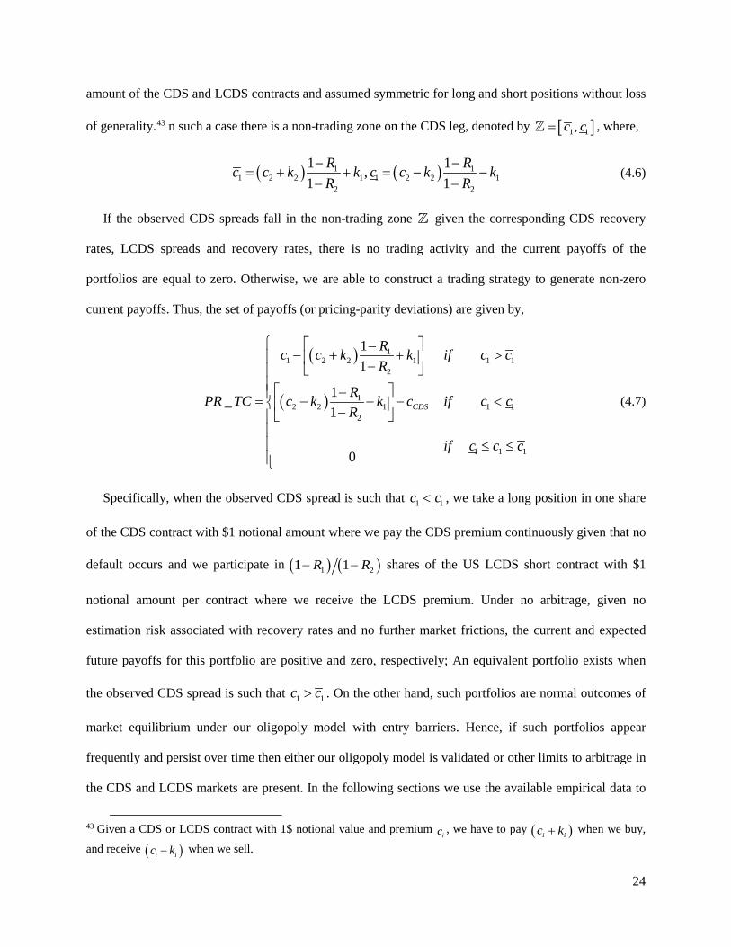
amount of the CDS and LCDS contracts and assumed symmetric for long and short positions without loss
of generality.43 n such a case there is a non-trading zone on the CDS leg, denoted by [ ]1 1,c c= , where,
( ) ( )1 11 2 2 1 1 2 2 1
2 2
1 1,1 1
R Rc c k k c c k kR R
− −= + + = − −
− − (4.6)
If the observed CDS spreads fall in the non-trading zone given the corresponding CDS recovery
rates, LCDS spreads and recovery rates, there is no trading activity and the current payoffs of the
portfolios are equal to zero. Otherwise, we are able to construct a trading strategy to generate non-zero
current payoffs. Thus, the set of payoffs (or pricing-parity deviations) are given by,
( )
( )
11 2 2 1 1 1
2
12 2 1 1 1
2
1 1 1
11
1_1
0
CDS
Rc c k k if c cR
RPR TC c k k c if c cR
if c c c
−− + + > −
−= − − − < − ≤ ≤
(4.7)
Specifically, when the observed CDS spread is such that 1 1c c< , we take a long position in one share
of the CDS contract with $1 notional amount where we pay the CDS premium continuously given that no
default occurs and we participate in ( ) ( )1 21 1R R− − shares of the US LCDS short contract with $1
notional amount per contract where we receive the LCDS premium. Under no arbitrage, given no
estimation risk associated with recovery rates and no further market frictions, the current and expected
future payoffs for this portfolio are positive and zero, respectively; An equivalent portfolio exists when
the observed CDS spread is such that 1 1c c> . On the other hand, such portfolios are normal outcomes of
market equilibrium under our oligopoly model with entry barriers. Hence, if such portfolios appear
frequently and persist over time then either our oligopoly model is validated or other limits to arbitrage in
the CDS and LCDS markets are present. In the following sections we use the available empirical data to
43 Given a CDS or LCDS contract with 1$ notional value and premium ic , we have to pay ( )i ic k+ when we buy,
and receive ( )i ic k− when we sell.
24

test the violations of parity between the two markets and attribute them to the relaxation of the
appropriate assumptions.
5. THE MAIN EMPIRICAL TESTS: PRICING PARITY VIOLATIONS
In this section we examine the current deviations of the CDS and LCDS parity relation developed in
the previous section, which are anomalous under no arbitrage but imply a non-competitive structure in our
oligopoly model. We verify whether these deviations lead to frequent positive payoff portfolio strategies
and, if yes, what factors may account for these payoffs. The results are presented both without and with
transaction costs. In subsequent sections we present further direct tests of the competing no arbitrage and
non-competitive structure hypotheses and we also examine whether the positive payoffs are due to our
assumptions of certain recovery rates or to the absence of limits to arbitrage.
5.1 Trading Strategies
Following the CDS and LCDS parity in the presence and in the absence of transaction costs discussed
in previous sections, we first examine the current payoffs in (4.7) with the observed CDS and LCDS data.
Figure 1 reports the distribution of simulated portfolio strategies with transaction costs.44
[Insert Figure 1 about here]
In the presence of transaction costs estimated from actual CDS data (see below) we observe that only
approximately 19% of the cross-sectional observations in the full sample fall in the no-trading zone
and cannot generate positive current payoffs. In both cases, with and without transaction costs, buying
CDS contracts and selling the corresponding LCDS contracts dominates the reverse trading strategy.
5.2 Current Payoffs of Liquid Portfolios with Transaction Costs
In this subsection we analyze the current payoffs of our portfolio strategies assuming that the recovery
rates reported by the Markit database are the “real recovery rates” once the default events occur.
[Insert Table 2 about here]
44 The summary statistics of one-way proportional transaction costs, the time trend of bid-ask spreads and the distribution of simulated trading strategies without transaction costs are reported in Table I, Figure I and Figure II in the online appendix, respectively.
25
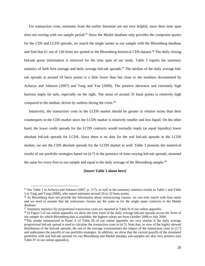
For transaction costs, estimates from the earlier literature are not very helpful, since their time span
does not overlap with our sample period.45 Since the Markit database only provides the composite quotes
for the CDS and LCDS spreads, we match the single names in our sample with the Bloomberg database
and find that 61 out of 120 firms are quoted in the Bloomberg historical CDS dataset.46 The daily closing
bid-ask quote information is retrieved for the time span of our study. Table 2 reports the summary
statistics of both firm average and daily average bid-ask spreads.47 The median of the daily average bid-
ask spreads at around 18 basis points is a little lower than but close to the numbers documented by
Acharya and Johnson (2007) and Tang and Yan (2008). The positive skewness and extremely high
kurtosis imply fat tails, especially on the right. The mean of around 35 basis points is relatively high
compared to the median, driven by outliers during the crisis.48
Intuitively, the transaction costs in the LCDS market should be greater in relative terms than their
counterparts in the CDS market since the LCDS market is relatively smaller and less liquid. On the other
hand, the lower credit spreads for the LCDS contracts would normally imply (at equal liquidity) lower
absolute bid-ask spreads for LCDS. Since there is no data for the real bid-ask spreads in the LCDS
market, we use the CDS absolute spreads for the LCDS market as well. Table 3 presents the numerical
results of our portfolio strategies based on (4.7) in the presence of time-varying bid-ask spreads, assumed
the same for every firm in our sample and equal to the daily average of the Bloomberg sample.49
[Insert Table 3 about here]
45 See Table 1 in Acharya and Johnson (2007, p. 117), as well as the summary statistics results in Table 1 and Table 3 in Tang and Yang (2008), who report estimates around 20 or 22 basis points. 46 As Bloomberg does not provide the information about restructuring clauses, we can only match with firm name and we need to assume that the restructure clauses are the same as for the single name contracts in the Markit database. 47 Summary statistics for proportional transaction costs are reported in Table II of our online appendix. 48 In Figure I of our online appendix we show the time trend of the daily average bid-ask spreads across the firms of our sample for which Bloomberg data is available; the highest values are from October 2008 to July 2009. 49The results summarized in Panel A of Table III of our online appendix are very similar if the daily average proportional bid-ask spread is used to calculate the transaction costs in (4.7). Note that, in view of the highly skewed distribution of the bid-ask spreads, the use of the average overestimates the impact of the transaction costs in (2.7) and understates the payoffs of our portfolio strategies. In addition, we show that the current payoffs of the simulated portfolios with real bid-ask spreads for our Bloomberg and Markit intraday sub-samples are also very positive (see Table IV in our online appendix).
26
Table 3 reports the payoffs of our simulated portfolios with transaction costs. The mean and median
returns increase as the rating status deteriorates, with the not-rated contracts generating the highest current
payoffs among all the sub-samples. As the time span of the single name contracts varies, the cross-
sectional average puts more weight on the firms with longer lives. To remove this bias, we first calculate
the daily average current payoffs for each single name across the life of the contract and then present the
statistical properties of the sample reported as “Firm Daily Average Current Payoffs”. The distribution
has a 4.5% mean and 2.5% median return, which are even greater than those based on the cross-sectional
observations.
[Insert Figure 2 about here]
To check the time trend of the current payoffs, we aggregate the value of current payoffs per day
across all the available paired single name contracts on that day and then divide by the total number of
single name contracts per day to construct a payoff index. As expected, the distribution of index returns is
almost Gaussian for all the samples. As in the cross-sectional results, the average current payoff increases
as the rating deteriorates, and the not-rated sub-sample dominates in terms of the mean and median of all
the rated sub-samples but also has the highest standard deviation, 3.16%. The time trend of daily average
current payoffs of the different samples can be observed in Figure 2, both with and without transaction
costs, with the two cases being very close to each other. In the full and investment grade samples we note
that the current payoffs are relatively higher during the recession period from mid-2008 to late 2009
compared to the other time periods, and gradually decrease in recent years. The junk-rated and not-rated
samples have significantly higher volatilities than the investment grade firms. Both junk-rated and not-
rated firms sub-samples are small firms in terms of total assets and have relatively lower tangible ratios
which make them more vulnerable, especially in turbulent financial market environments. These style
factors contribute to the higher volatilities for these two sub-samples compared to the investment grade
firms.
27
5.3 A Naïve Trading Strategy
While the estimated CDS and LCDS recovery rates are inputs to justify the choice of trading strategy,
it is impossible to observe the real recovery rates until a firm defaults. In this robustness test, we rule out
this uncertainty from the trading strategy selection process and pursue a naïve trading strategy under
which we always pay the CDS premium and receive the corresponding LCDS premium. Interestingly, we
are still able to document daily abnormal current deviations in terms of their mean and median of
approximately 1.52% and 0.64%, respectively, for the full sample.
Summarizing our numerical results, we note that the observed CDS and LCDS prices do not satisfy the
no arbitrage parity relation (4.5), even with the inclusion of generous transaction costs as in (4.6)-(4.7).
They show that in most cases (but not always) that the LCDS contracts are over-valued, and that taking
advantage of the recovery rate estimates improves the profitability of trading strategies.
5.4 Possible Explanations
If a zero net cost portfolio generates positive payoffs in a no arbitrage model then there are three
possible reasons. The most commonly invoked justification is that the payoffs are rewards for risk. Unlike
other similar arbitrage-like strategies involving different financial instruments in which model error is
always present, such risk is relatively easy to evaluate in our case. It appears only in the case where the
underlying firm defaults prior to contract maturity, and arises either from incorrect estimates of the
recovery rates in (4.7) or from counterparty default. Alternative explanations in a no arbitrage context are
the often invoked limits to arbitrage such as margins, liquidity, or slow moving capital. 50 With the
exception of the latter factor, the others are also characteristics of a non-competitive market structure and
have been incorporated into our oligopoly model of Section 3. We deal with each in turn.
5.5 Reward for Risk? Evidence from Matured Contracts
For the payoffs to be rewards for risk the portfolio strategies must occasionally produce losses at
contract maturity. Although it is not possible to observe ex post the payoffs of our portfolios for the 5-
year CDS-LCDS contract pairs, such verification is feasible for subsets of our 1- and 3-year samples.
50 Shleifer and Vishny (1997), Mitchell, Pulvino and Stafford (2002), and Duffie (2010).
28
Since the screening rule for profitable portfolios on the basis of the available data is identical for these
short term contracts and our 5-year sample, the reliability of the recovery rate estimates can be assessed
from the matured contracts. For the one-year subsample ending on March 19, 2011 there are 31,493
observations consisting of 70 firms between April 11, 2008 and March 19, 2011, of which 11,425
observations are after April 5, 2010, when the LCDS contracts became fully non-cancellable. Using
Moody’s default and recovery data base, we find four default events on three firms because of distressed
exchange.51 In all cases the observed recovery rates maintain or enhance the payoffs of the portfolios
selected by the estimated recovery rates in the Markit data base. Assuming the average trading size of a
CDS contract of $5 million according to the empirical data, we calculate the dollar trading profit after
incorporating the transaction costs for each contract.52 For simplicity, we ignore the time value of money
and find that the 1-year sample could generate around $3.272 billion in profits using our CDS-LCDS
parity trading strategy.
A similar picture emerges when we examine the 3-year contracts ending on March 19, 2009, for which
our sample covers the entire life of the contracts. This 3-year subsample consists of 7397 contracts on 61
firms. After verifying the few recorded defaults according to Moody’s default and recovery database we
apply the same payoff estimation and find that all contracts were profitable. Using again the same average
CDS contract size and ignoring the rate of interest, we document approximately $3.652 billion in
abnormal profits.
In other words, out of a sample of more than 18,000 observations capable of generating more than
$6.9 billion of profits from our zero net cost portfolio strategies there was not a single instance of
recorded losses. With such results the reward for risk explanation is not credible and must be discarded:
positive payoffs may not be arbitrage profits theoretically, but they are certainly such profits in a
statistical sense. Nonetheless, we re-examine in our robustness checks and our online appendix both
51 CCU on Aug, 27th, 2009 with real recovery rates 32%, LVLT on Dec 23rd, 2008 and Jun 26th, 2009 with real recovery rates 96% and 100% and UIS on July 31st, 2009 with real recovery rates 99%. 52 We consider each observation as an independent contract on each day. A default event of a firm triggers the payments of all the on-going CDS contracts. The loss given default is paid based on the real recovery rates reported in Moody’s dataset. Meanwhile, all the CDS premiums stop on such firms upon the arrival of default.
29
recovery rate uncertainty and counterparty risk for our five-year contracts, which is discussed in detail in
Section 7.
5.6 Limits to Arbitrage or Non-Competitive Market Structure?
The alternative explanations of limits to arbitrage or non-competitive market structure are qualitatively
very different justifications for the observed positive payoffs. The former accepts the validity of (4.5) in
the frictionless markets and expands the definition of trading frictions beyond (4.6)-(4.7) to demonstrate
the inability of inter-market trading to take advantage of its violations. The latter demonstrates that (4.5)
does not hold if either one of the two markets is non-competitive, and attributes the payoffs to the
inability of competition to eliminate the profits. In fact, however, the two alternative explanations blur at
the edges, as we showed in our oligopoly model of Section 3. For instance, illiquid markets, a cornerstone
of the limits to arbitrage approach, imply that entering into a market in a timely manner would impact the
price, as in the net demand functions of Section 3, unlike the infinitely elastic demand curves of perfect
competition. Nonetheless, under limits to arbitrage the positive payoffs are anomalous and the markets
should converge to the no trading zone, unlike oligopoly. We examine these issues in the next section.
6. EMPIRICAL TESTS OF MARKET STRUCTURE AND LIMITS TO ARBITRAGE
6.1 Control Variables Affecting the Integration of the Two Markets
Before testing the competing hypotheses we need to control for both firm-specific and macro variables
that affect market conditions. These are chosen from the existing credit spreads literature, 53 after
reflecting multicollinearity 54 and data availability. These variables are particularly important in the
oligopoly model, since they affect the parity relation through the demand curves in both markets, in
addition to the recovery rates. The latter are the only ones affected under the no arbitrage hypothesis.55
53 See Collin-Dufresne, Goldstein and Spencer (2001), Acharya, Bharath and Srinivasan (2007), Acharya and Johnson (2007), Ericsson, Jacobs and Oviedo (2009) and Cao, Yu and Zhong (2010). 54 For instance, we use the yields on 5-year US treasury bonds since both CDS and LCDS contracts in our sample have five years to maturity. We use the spread between the yields on Aaa and Baa corporate bonds (CBS) and eliminate the VIX because we find that these two variables are highly correlated and that the CBS has better explanatory power than VIX. The correlations between the variables are reported in Table XI in the online appendix. 55 We also expect under both hypotheses a widening of the no trading zone during the crisis because of the increase in transaction costs.
30
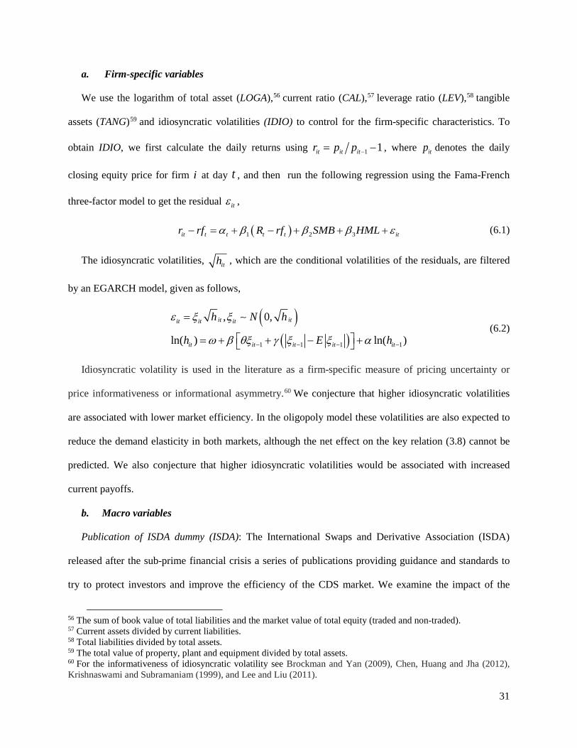
a. Firm-specific variables
We use the logarithm of total asset (LOGA),56 current ratio (CAL),57 leverage ratio (LEV),58 tangible
assets (TANG)59 and idiosyncratic volatilities (IDIO) to control for the firm-specific characteristics. To
obtain IDIO, we first calculate the daily returns using 1 1it it itr p p −= − , where itp denotes the daily
closing equity price for firm i at day t , and then run the following regression using the Fama-French
three-factor model to get the residual itε ,
( )1 2 3it t t t t itr rf R rf SMB HMLα β β β ε− = + − + + + (6.1)
The idiosyncratic volatilities, ith , which are the conditional volatilities of the residuals, are filtered
by an EGARCH model, given as follows,
( )
( )1 1 1 1
, 0,
ln( ) ln( )
it itit it it
it it it it it
h N h
h E h
ε ξ ξ
ω β θξ γ ξ ξ α− − − −
=
= + + − +
(6.2)
Idiosyncratic volatility is used in the literature as a firm-specific measure of pricing uncertainty or
price informativeness or informational asymmetry.60 We conjecture that higher idiosyncratic volatilities
are associated with lower market efficiency. In the oligopoly model these volatilities are also expected to
reduce the demand elasticity in both markets, although the net effect on the key relation (3.8) cannot be
predicted. We also conjecture that higher idiosyncratic volatilities would be associated with increased
current payoffs.
b. Macro variables
Publication of ISDA dummy (ISDA): The International Swaps and Derivative Association (ISDA)
released after the sub-prime financial crisis a series of publications providing guidance and standards to
try to protect investors and improve the efficiency of the CDS market. We examine the impact of the
56 The sum of book value of total liabilities and the market value of total equity (traded and non-traded). 57 Current assets divided by current liabilities. 58 Total liabilities divided by total assets. 59 The total value of property, plant and equipment divided by total assets. 60 For the informativeness of idiosyncratic volatility see Brockman and Yan (2009), Chen, Huang and Jha (2012), Krishnaswami and Subramaniam (1999), and Lee and Liu (2011).
31
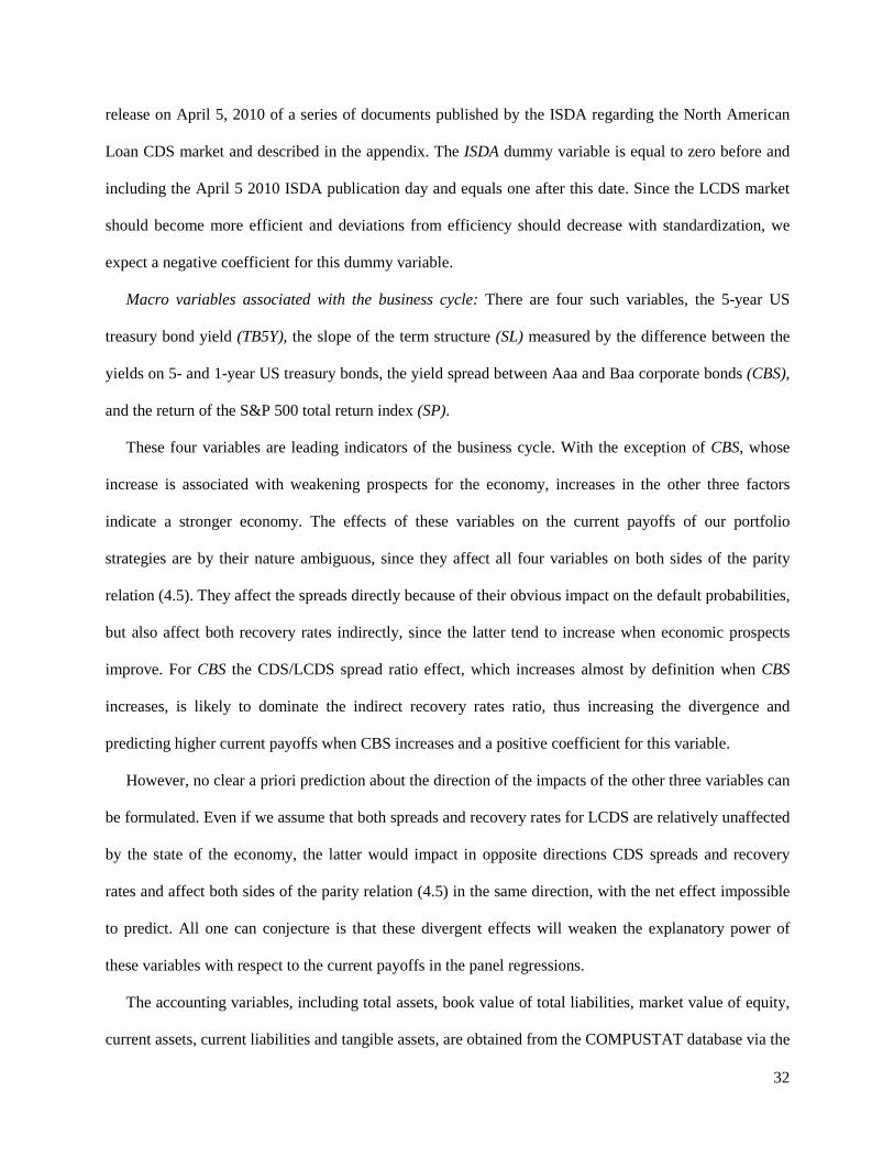
release on April 5, 2010 of a series of documents published by the ISDA regarding the North American
Loan CDS market and described in the appendix. The ISDA dummy variable is equal to zero before and
including the April 5 2010 ISDA publication day and equals one after this date. Since the LCDS market
should become more efficient and deviations from efficiency should decrease with standardization, we
expect a negative coefficient for this dummy variable.
Macro variables associated with the business cycle: There are four such variables, the 5-year US
treasury bond yield (TB5Y), the slope of the term structure (SL) measured by the difference between the
yields on 5- and 1-year US treasury bonds, the yield spread between Aaa and Baa corporate bonds (CBS),
and the return of the S&P 500 total return index (SP).
These four variables are leading indicators of the business cycle. With the exception of CBS, whose
increase is associated with weakening prospects for the economy, increases in the other three factors
indicate a stronger economy. The effects of these variables on the current payoffs of our portfolio
strategies are by their nature ambiguous, since they affect all four variables on both sides of the parity
relation (4.5). They affect the spreads directly because of their obvious impact on the default probabilities,
but also affect both recovery rates indirectly, since the latter tend to increase when economic prospects
improve. For CBS the CDS/LCDS spread ratio effect, which increases almost by definition when CBS
increases, is likely to dominate the indirect recovery rates ratio, thus increasing the divergence and
predicting higher current payoffs when CBS increases and a positive coefficient for this variable.
However, no clear a priori prediction about the direction of the impacts of the other three variables can
be formulated. Even if we assume that both spreads and recovery rates for LCDS are relatively unaffected
by the state of the economy, the latter would impact in opposite directions CDS spreads and recovery
rates and affect both sides of the parity relation (4.5) in the same direction, with the net effect impossible
to predict. All one can conjecture is that these divergent effects will weaken the explanatory power of
these variables with respect to the current payoffs in the panel regressions.
The accounting variables, including total assets, book value of total liabilities, market value of equity,
current assets, current liabilities and tangible assets, are obtained from the COMPUSTAT database via the
32

WRDS platform. The data are updated quarterly. For our initial regressions, we convert the frequency
from quarterly to daily by keeping the value constant within each quarter and then take a one quarter lag.
The fixed income macro variables, including the yields on 1- and 5-year US treasury bonds, and Aaa and
Baa corporate bond yields are obtained from the US Federal Reserve H15 database. The equity prices and
S&P 500 total return index data are obtained from Bloomberg.
6.2 Market Structure Hypotheses
Equation (3.7) is the key empirical relation. The right-hand-side (RHS) is observable as an estimate
(assumed unbiased), while in the left-hand-side the observable ratio of the spreads is multiplied by the
unobservable ratio of the modified elasticities, 1 2 1
1 2
2
1(1 )(1 )
1 (1 )(1 )D D D
D D
D
J JJ
J
ε ε εε ε
ε
++
=++
. Note that J is the number of
arbitrageurs common to both markets. An imperfect proxy, an upper bound of this number, is the
minimum of the number of quotes in the CDS or LCDS markets in a given day. As for the other traders
beyond the minimum, they obviously are participants in only one market and can be included in the
definition of net demand.
The derivative with respect to J of the ratio 1
2
11
D
D
JJεε
++
has the sign of the difference 2 1D Dε ε− , which
we cannot infer a priori for the two markets. However, we can surmise that this difference, as well as the
ratio of the elasticities, will increase as the difference in the number of traders in the two markets
increases. Also, the profits from arbitrage should increase as J decreases. We construct the following
two hypotheses to test the empirical implications from the market power hypothesis:
H1: The profits from the parity violations will increase as the minimum number of quotes in the two
markets decreases.
H2: The parity violations profits will widen as the difference in the number of quotes rises.
[Insert Table 4 about here]
33
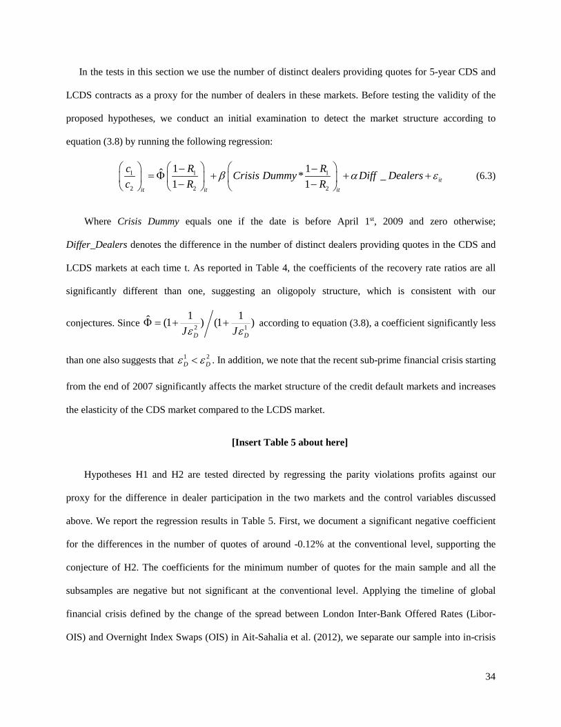
In the tests in this section we use the number of distinct dealers providing quotes for 5-year CDS and
LCDS contracts as a proxy for the number of dealers in these markets. Before testing the validity of the
proposed hypotheses, we conduct an initial examination to detect the market structure according to
equation (3.8) by running the following regression:
1 1 1
2 2 2
1 1ˆ * _1 1 it
it it it
c R RCrisis Dummy Diff Dealersc R R
β α ε − −
= Φ + + + − − (6.3)
Where Crisis Dummy equals one if the date is before April 1st, 2009 and zero otherwise;
Differ_Dealers denotes the difference in the number of distinct dealers providing quotes in the CDS and
LCDS markets at each time t. As reported in Table 4, the coefficients of the recovery rate ratios are all
significantly different than one, suggesting an oligopoly structure, which is consistent with our
conjectures. Since 2 11 1ˆ (1 ) (1 )
D DJ Jε εΦ = + + according to equation (3.8), a coefficient significantly less
than one also suggests that 1 2D Dε ε< . In addition, we note that the recent sub-prime financial crisis starting
from the end of 2007 significantly affects the market structure of the credit default markets and increases
the elasticity of the CDS market compared to the LCDS market.
[Insert Table 5 about here]
Hypotheses H1 and H2 are tested directed by regressing the parity violations profits against our
proxy for the difference in dealer participation in the two markets and the control variables discussed
above. We report the regression results in Table 5. First, we document a significant negative coefficient
for the differences in the number of quotes of around -0.12% at the conventional level, supporting the
conjecture of H2. The coefficients for the minimum number of quotes for the main sample and all the
subsamples are negative but not significant at the conventional level. Applying the timeline of global
financial crisis defined by the change of the spread between London Inter-Bank Offered Rates (Libor-
OIS) and Overnight Index Swaps (OIS) in Ait-Sahalia et al. (2012), we separate our sample into in-crisis
34
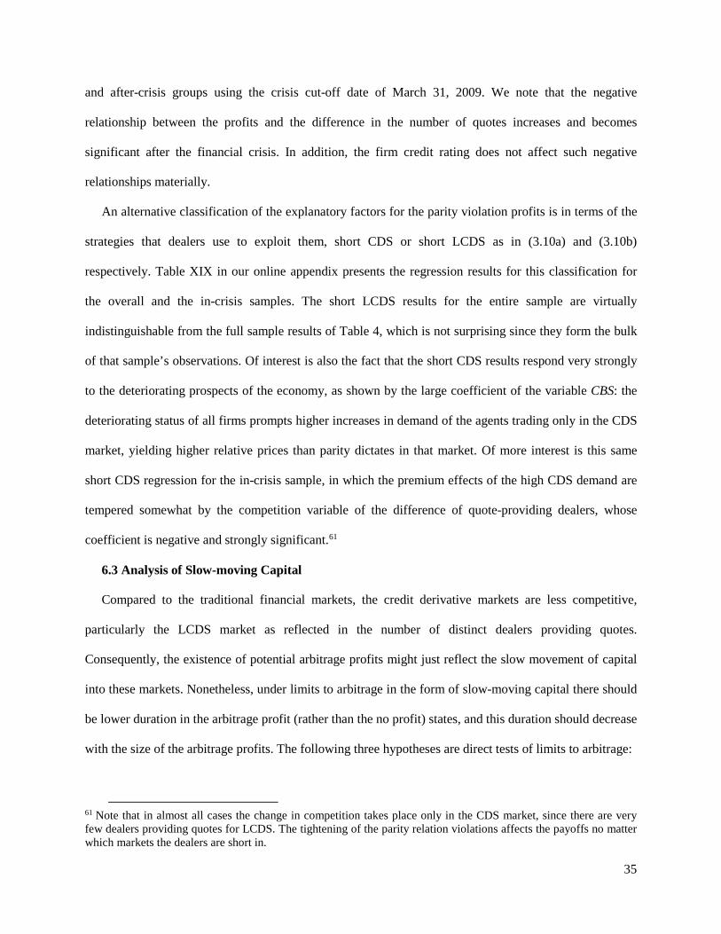
and after-crisis groups using the crisis cut-off date of March 31, 2009. We note that the negative
relationship between the profits and the difference in the number of quotes increases and becomes
significant after the financial crisis. In addition, the firm credit rating does not affect such negative
relationships materially.
An alternative classification of the explanatory factors for the parity violation profits is in terms of the
strategies that dealers use to exploit them, short CDS or short LCDS as in (3.10a) and (3.10b)
respectively. Table XIX in our online appendix presents the regression results for this classification for
the overall and the in-crisis samples. The short LCDS results for the entire sample are virtually
indistinguishable from the full sample results of Table 4, which is not surprising since they form the bulk
of that sample’s observations. Of interest is also the fact that the short CDS results respond very strongly
to the deteriorating prospects of the economy, as shown by the large coefficient of the variable CBS: the
deteriorating status of all firms prompts higher increases in demand of the agents trading only in the CDS
market, yielding higher relative prices than parity dictates in that market. Of more interest is this same
short CDS regression for the in-crisis sample, in which the premium effects of the high CDS demand are
tempered somewhat by the competition variable of the difference of quote-providing dealers, whose
coefficient is negative and strongly significant.61
6.3 Analysis of Slow-moving Capital
Compared to the traditional financial markets, the credit derivative markets are less competitive,
particularly the LCDS market as reflected in the number of distinct dealers providing quotes.
Consequently, the existence of potential arbitrage profits might just reflect the slow movement of capital
into these markets. Nonetheless, under limits to arbitrage in the form of slow-moving capital there should
be lower duration in the arbitrage profit (rather than the no profit) states, and this duration should decrease
with the size of the arbitrage profits. The following three hypotheses are direct tests of limits to arbitrage:
61 Note that in almost all cases the change in competition takes place only in the CDS market, since there are very few dealers providing quotes for LCDS. The tightening of the parity relation violations affects the payoffs no matter which markets the dealers are short in.
35

H3: The persistence of observed arbitrage profits states is lower than that of absence of profits
states.
H4: The duration of arbitrage profits states decreases with the size of observed profits.
H5: In arbitrage profits states the CDS and LCDS premiums should change in the direction of the
elimination of profits.
[Insert Table 6 about here]
To test H3 we count the number of consecutive days on which a particular CDS-LCDS pair persists in
an arbitrage profit or no-profit state once we observe an arbitrage profit opportunity (or lack thereof)
according to the CDS-LCDS parity rule presented in the previous sections. Based on the results reported
in Table 6, we find that the median number of days of persistence or duration of arbitrage profits is 5 (3)
days when the CDS contracts are much cheaper (more expensive) compared to their corresponding LCDS
contracts. Interestingly, the shortest period is for the no-profit state, and especially for the no-rating
subsample. The extremely high mean of about 52 days for the majority case is driven by some extreme
cases and strong positive skewness since this variable is truncated at zero. The no-rating subsample and
the post-crisis period show the highest persistence in one of the profit states and the lowest persistence in
the no-profit state. In other words, the market seems to respond fastest to the absence, rather than the
presence of parity violations, directly contradicting H3. Also, the parity violations are not related to the
crisis.
[Insert Table 7 about here]
To test H4 we estimate a panel regression with single-name fixed effects that adds arbitrage profits on
the day first observed (Profit_TC) as an independent variable. The dependent variable measures the
duration of the persistence of arbitrage profits by the number of consecutive days for which the arbitrage
profits continue to be positive after first observed. This persistence measure is winsorized at the 5% and
95% levels to mitigate the impact of extreme values. Our expectation is that the coefficient estimates for
Profit_TC should be negative if H4 holds, since capital should move faster in response to higher arbitrage
36
profit opportunities. Based on the results reported in Table 7, we observe positive estimated coefficients
for Profit_TC that are significant at the 0.05 level or better for all but the speculative subsample
(significant at 0.10 level). Thus H4 is decisively rejected, in contradiction to the slow-moving capital or,
indeed, to any other limits to arbitrage factors. The duration of arbitrage profits increases with an increase
in the magnitude of arbitrage profits as predicted by the oligopoly market model. This result is the single
most powerful rejection of limits to arbitrage and support for the financial oligopoly hypothesis.
Last, for H5 we construct a diverging ratio to measure the persistence of all the possible arbitrage
opportunities based on parity violations. This measure is inspired by the K-metric developed in Kapadia
and Pu (2012). Assume that we have 1, ...,l N= pairs of CDS and LCDS contracts on a given date and
the total number of periods in our sample is denoted by τ , where 1 N kτ≤ ≤ − and k M τ≤ − .
According to equation (4.7) with proportional transaction costs, we define,
( )
( )
1111
U CDSCDS LCDS LCDS CDS
LCDS
L CDSCDS LCDS LCDS CDS
LCDS
Rc c k kRRc c k kR
−= + +
−−
= − −−
(6.4)
If we observe LCDS CDSc c< on day 0, we define the diverging changes as,
0, 00, 00, 0
LCDS CDS
L LCDS CDS CDS CDS
L LCDS CDS CDS CDS
c cc c and c cc c and c c
∆ < ∆ >∆ > ∆ > ∆ < ∆∆ < ∆ < ∆ > ∆
(6.5)
Where CDSc∆ and LCDSc∆ denote the change of CDS and LCDS spreads. If we observe UCDS CDSc c>
instead, we define the diverging changes as,
0, 00, 00, 0
UCDS CDS
U UCDS CDS CDS CDS
U UCDS CDS CDS CDS
c cc c and c cc c and c c
∆ > ∆ <∆ > ∆ > ∆ > ∆∆ < ∆ < ∆ < ∆
(6.6)
We define the diverging ratios as,
37
[ ]
( )
1
1 1
1
N N
Diverging ChangekDR
N N
τ
τ
− −
= ==−
∑∑1 (6.7)
This nonparametric measure is independent of the time period since it accounts for all the pairings of
CDS and LCDS and all the possible combinations from the N observations. Furthermore, this measure is
based on standard statistical properties and is not impacted by nonlinearities.
[Insert Table 8 about here]
Descriptive statistics are reported in Table 8 for the diverging ratios (DR) calculated using the
overlapping windows with varying window sizes for each firm. The diverging ratios for the full sample
only vary slightly from 5 to 60 days, implying persistence in the arbitrage opportunities in the CDS and
LCDS markets. This finding is robust for sub-samples based on credit ratings or position in the economic
cycle. These results show conclusively that there is no pattern in the movements of the relative spreads in
connection to the observed parity violations, directly contradicting H5. The median DR is around 50% for
the full sample in all cases, both in- and post-crisis.
6.4 Conclusions of the Empirical Tests
As noted in Section 4, of the three competing explanations for the pricing parity violations only limits
to arbitrage and market structure remain after the elimination of the observed profits as rewards for risk.
Although limits to arbitrage is the most popular explanation among finance researchers for such
violations, the evidence for the existence of an oligopolistic structure in all CDS markets at the dealer
level provided in Section 2 is conclusive and cannot be ignored. The effect of such an oligopoly is
demonstrated in Section 3, in which the pricing parity violations and trading profits are present even in
the absence of collusion. The empirical evidence in this section overwhelmingly supports this oligopoly
model, since limits to arbitrage are inconsistent with the observed absence or perverse market response to
the observed pricing parity violations and to the sensitivity of the violations to the competitive status of
the CDS markets.
38

7. ROBUSTNESS CHECKS
In this section and in our online appendix we revisit the justification of the observed parity violations
and positive portfolio payoffs as rewards for risk. As we saw, such a justification is not warranted for the
one- and three-year contracts, but it may have some credibility for the more liquid five-year contracts that
form the bulk of our data and empirical work. Accepting the reward for risk explanation for the observed
payoffs essentially implies that the screening rule (4.6)-(4.7) for mispriced contracts is unreliable. Since,
unlike other similar arbitrages in the financial literature,62 the recovery rates in the Markit data base are
the only estimates of unobservable factors in the relations, their reliability needs to be verified. This is
done in the next subsection, while subsections 7.2 and 7.3 deal with liquidity and counterparty risk in the
limits to arbitrage scenario.
7.1 Uncertainty of Recovery Rates: Quality and Bias of the Markit Estimates
a. Impact of Absolute Priority Rule
The priority of the LCDS over the CDS claims in the event of default is a key issue in assessing the
future payoffs of our portfolios in case a default event occurs. As a rule, syndicated secured loans have
claim priority compared to the senior unsecured debts implying a 100% recovery for LCDS-underlying
loans before the recovery for CDS debts can become positive. To understand the role of such priority, we
denote by rCDSR and r
LCDSR the realized (as distinct from the Markit estimates) recovery rates at default
and consider the future payoffs of portfolios such that CDS CDSc c< in (4.7). The payoff to that portfolio in
the event of default is
1 11 (1 ) 1 (1 )1 1
rr r rCDS LCDSCDS LCDS CDS CDS
LCDS LCDS
R RR R R RR R
− −− − − = − − −
− − (7.1)
If there is no error in the estimate LCDSR then the payoff is equal to rCDS CDSR R− . Similarly, the
payoff is always nonnegative whenever 100%rLCDSR = and strictly positive if 0r
CDSR = and
rLCDS LCDSR R≥ . In other words, these portfolios, in addition to the current positive payoffs, have always
62 See, for instance, the model-based arbitrage strategies in Duarte, Longstaff and Yu (2007).
39

nonnegative future payoffs under LCDS priority and full recovery. To evaluate the impact of LCDS
priority in the event of default we relax the assumption that LCDSR is an accurate estimate of the real
recovery rates for the LCDS-underlying assets. The data and details of the tests are reported in Table IX
of our online appendix.
Overall, the data in that table strongly suggests that our potential payoffs from pricing parity
deviations which are based on the Markit data base estimates of both CDS and LCDS recovery rates are,
if anything, highly conservative. Recall that when concurrent default occurs, we receive in the
overwhelming majority of pricing parity violations cases the loss given default on the CDS leg and pay
the loss given default on the LCDS leg, as in relation (4.7).
Hence, the available empirical evidence about the real recovery rates implies that in the overwhelming
majority of cases the current payoffs on the simulated portfolio will be augmented by future payoffs when
default occurs, thus increasing the profitability of our portfolio strategy. Such a conclusion implies, in
turn, that in the absence of liquidity considerations the observed structure of the premiums in the CDS
and LCDS markets indicate that trading in the two markets takes place without taking into account the
LCDS priority rule in the event of default. Such segmentation is present in the oligopoly model of Section
3, due to the barriers to entry at the dealer level.63
On the other hand, the future payoffs upon default will be negative for the portfolios that pay the
LCDS and receive the CDS premium. Apart from the fact that these cases are relatively few, they do not
necessarily negate the observed abnormal current payoffs. The reason is that all one has to do is refrain
from trading in these cases if the evidence from Table 3 is confirmed with more extensive data on actual
defaults and recoveries. These cases are analyzed further in our online appendix, where it is shown that
they offer further supportive evidence of market segmentation.
b. Structural Model Implied Recovery Rates
63 Similar anomalous relations have been observed in the index and equity option markets by Driessen, Maenhout and Vilkov (2009) and the index futures options and underlying market by Constantinides et al (2011).
40

We also verify whether our results hold when we estimate the recovery rate by a structural no arbitrage
model that treats corporate debt and equity as contingent claims on the firm’s assets and links default risk
and firm characteristics. We combine the information from different financial markets, including equity
and option markets, with accounting information to calculate the model implied recovery rates and search
for pricing-parity violations with these new recovery rates. We also obtain estimates of the expected
future payoffs upon default, analyzed in the next subsection.
Our structural model is the one presented in Leland and Toft (1996). Although this model’s capital
structure differs from the structure of the firms in our sample, it is the most popular bond pricing
structural model in the literature and has two important advantages. First, Leland and Toft (1996) use the
endogenous default boundary that is chosen by the firm itself, and second it presents closed form
expressions for all the variables of interest, which provide significant computational convenience for the
estimation. The details of the model, the data description and the Generalized Method of Moments
(GMM) procedures are reported in our online appendix.
[Insert Table 9 about Here]
Table 9 reports the results of the GMM estimations and the new current payoffs using the implied
CDS recovery rates from the structural model. In Panel A, the implied CDS recovery rates on average are
very close to the estimates provided by the Markit datasets, especially the results (around 35%) using put
option implied equity volatilities. The high standard deviation of 25.34% and 24.22% for results with
option implied volatilities and realized volatilities respectively, across all the firms indicates that the
cross-sectional effect is very important. The asset volatilities are approximately 10% under both option
implied and realized volatilities and are very persistent across all the firms as indicated by the low
standard deviations.
41
Using the model implied CDS recovery rates as being constant across the whole time period for each
firm,64 we repeat the computations of the current payoffs and report the results in Panels B and C for
option implied and realized equity volatilities, respectively. Compared to the current payoffs under the
estimated recovery rates (see Panel B of Table 2), the means of the current payoffs under the structural
model implied CDS recovery rates are much lower at 2.74% and 2.83% for option implied and realized
equity volatilities, respectively, but the corresponding medians are much higher at 1.35% and 1.44%,
respectively, for the cross-sectional daily observations. In addition, the results are very similar for both
the firm average and daily average samples. These positive and large abnormal current payoffs on the
portfolios, evaluated under two very different methods that use partly different data sets, confirm the
failure of simultaneous trading in both markets to equalize the spreads in the CDS and LCDS markets.
7.2 Contract Liquidity and the Term Structure of the Portfolio Current Payoffs
The previous analyses focus mostly on the 5-year CDS and LCDS contracts which are the most liquid
contracts in these markets. In this section, we expand our sample to other maturities, including 1-year, 3-
year, 7-year and 10-year maturities. Due to the illiquidity and data availability of contracts for the other
maturities, the total number of cross-sectional observations is reduced from 69,805 to 33,377 after
deleting the observations with missing variables. If illiquidity of the contracts is the factor responsible for
the large current payoffs of the pricing parity violations portfolios then we should observe more of them
for these more illiquid contracts than for the 5-year ones.
[Insert Figure 3 and Figure 4 about here]
Figure 3 exhibits both the medians and means of the current payoffs on the portfolios consisting of
CDS and LCDS contract pairings across the different maturities in the presence of transaction costs.65
The distributions of these current payoffs across all the maturities are highly positively skewed since all
the means (around 2.8% in average size) are significantly greater than their corresponding medians
64 We use estimated LCDS recovery rates provided by Markit. As the underlying asset of LCDS is syndicated secured loans which usually have collateral backing and are senior to the senior unsecured debts, the recovery rates are much easier to estimate. 65 The transaction cost information represented by the bid-ask spreads is collected from Bloomberg for the different maturities.
42
(around 1% on average). There is a clear upward trend for the median current payoffs as the maturity
increases from 1 to 5 years before it becomes flat for the longer maturities. Nevertheless, the mean
payoffs exhibit a flat term structure. As the value of current payoffs on the portfolios with zero-expected
payoffs measure the deviations from the CDS and LCDS parity described in Section 1, we expect to
observe fewer violations of the parity relation for short-term contracts because of the reduced probability
of the default event during contract life.
Figure 4 shows the distribution of the trading strategies across all the maturities we considered. We
document that for the shortest (1-year) maturity approximately 35% of the observations, the highest
percentage among all the maturities, do not violate the CDS and LCDS parity, as expected; recall that for
these contracts all of our simulated portfolios in cases of violations turned out to be profitable. The
violation percentage increases as the maturity increases from 1 to 5 years and stays approximately
constant thereafter. Since the contracts with 5-year maturity are the most liquid ones in our sample, these
results suggest that contract illiquidity is not a factor in the incidence of parity violations. These results
actually constitute further evidence against limits of arbitrage and in favor of the oligopoly model in
which illiquidity is built into the model and explains the profitable strategies.
Across all the maturities, paying the CDS premium and receiving the corresponding LCDS premium
dominates the other trading strategies. This confirms our earlier findings that the observed CDS premiums
are too cheap given the corresponding LCDS premiums, and expected CDS and LCDS recovery rates. We
also note that the percentage of receiving CDS premiums and paying corresponding LCD premiums
slightly increases as the maturity increases from 1 to 7 years.
7.3 Counterparty Risk
Counterparty risk in a CDS market (i.e., the risk associated with a counterparty failing to honor its
obligations) was at the center of the 2008 financial crisis, which was caused in part by the near failure and
bailout of the American International Group (AIG), a leading seller of CDS contracts. As discussed in
Section 2, the evolving regulatory environment and the introduction of CCP’s and margins was in part
43
intended to eliminate it.66 Since it evolved during our data period and our data base does not distinguish
between trades that went through a CCP and the others, we cannot evaluate its role in explaining the
positive payoffs in a no arbitrage scenario. Nonetheless, since Arora, Gandhi and Longstaff (2012) find
that the magnitude of the counterparty risk that is priced is vanishingly small,67 the counterparty risk
premium might be able to explain only a very small portion of the abnormal current deviations when the
intermediate investor has lower credit risk than the CDS (LCDS) protection seller. Otherwise, the
counterparty risk should have no impact on CDS and LCDS parity due to the nature of the risk transfer.
7.4 Margins
When considering the role of margins as a barrier to entry, we first note that traders are allowed to net
out their margin positions, with the result that the collateral to gross notional ratio in CDS trades was
0.78% in 2001, which was far below the ICE margins, as noted in Duffie et al (2015). In the absence of
such data for the LCDS market and the identities of the traders in both markets it is not possible to assess
the net margin necessary for our pricing parity violations portfolios. Nonetheless, we conduct robustness
checks by examining the role of margins for the matured one-year contracts using the ICE margins under
the most adverse conditions.
[Insert Table 10 about here]
We consider scenarios with margin requirements from 0% up to 10% and a cost of capital from 5% to
10%. As indicated by a regulatory note from FINRA, the margin requirements for the short position are
much higher than the long position in credit default swap markets. To capture this differential
requirement, we include scenarios where the margin requirements for short positions are double those for
long positions. Given a 0.78% margin requirement, the aggregate dollar profits are $3.13 and $2.87
billion when the cost of capital is 5% and 10%, respectively, under the worst scenarios. Considering the
66 The impact of the central clearing counterparty (CCP) on the CDS market’s counterparty risk is unclear. For instance, Duffie and Zhu (2011) show an increase of counterpart risk in the presence of CCP while Loon and Zhong (2014) document a decrease. Due to the nature of counterparty risk transfer under our trading strategy, the presence of CCP should not be able to explain the documented abnormal current deviations documented herein. 67 Arora, Gandhi and Longstaff (2012) find an increase in the dealer’s credit spread of 645 basis points only translates into a one basis-point decrease in the CDS premium.
44
aggregate margin requirement of $5.27 billion, the annual returns are about 59.4% and 54.5%,
respectively, which are abnormally high. Hence, using a reasonable level of margin requirements does not
eliminate the abnormal profits documented for the matured contracts, even when the margin requirements
are double for short versus long positions. These results also show that margin requirements can act as a
barrier to entry since potential arbitrageurs with limited capital will be subject to the higher margins,
which along with a higher cost of capital due to less diversified portfolios will render the arbitrage trading
strategy tested herein unprofitable for them.
8. CONCLUSION
Based on the documented highly concentrated structure of the CDS markets, we formulate a Cournot-
style oligopoly model for intermarket trading in the CDS and LCDS markets on the same reference entity.
Such a model can explain the observed extensive violations of the CDS-LCDS parity relation, which
holds only under competitive conditions in both markets. In turn, these violations imply time-varying and
significant positive current payoffs from simulated portfolios that simultaneously take offsetting positions
in CDS and the corresponding LCDS contract depending on the direction of the violation of the parity
relation. We extend the oligopoly model to include proportional transaction costs. In such a case we show
that the parity relation includes a no trade zone and that the transaction costs constitute a barrier to small
scale entry that can be overcome by increasing the trader’s scale as measured by her start-up capital.
The observed abnormal positive current payoffs cannot be explained by data imperfections, risk of
future positions or limits to arbitrage such as transaction costs, illiquidity of contracts or counterparty risk,
but are consistent with our oligopoly model on the dealer side in both markets. We confirm these findings
with data from matured one- and three-year contracts that show uniformly positive realized profits of our
simulated portfolios and with extensive empirical tests that reject decisively the conventional limits to
arbitrage factors in favor of the competing oligopoly hypothesis. We examine the role of margins and
conclude that they constitute a barrier to the entry of small scale and/or undiversified traders.
45
This failure of intermarket trading to equalize the spreads in the CDS and LCDS markets is analyzed
theoretically and is formally documented here for the first time. Our theoretical and empirical analysis
confirms the related theoretical results by Atkeson et al (2013) and the conjectured and anecdotal
evidence by Bolton and Oemhke (2013), as well as the structure of CDS markets documented in Peltonen
et al (2014) and Duffie et al (2015). Note that the CDS markets’ highly concentrated nature is currently
the subject of an antitrust investigation by the European Commission.68,69
Our theoretical and empirical results also have regulatory implications which, however, are not clear
in the absence of detailed information and intraday data on actual margins, contract depths and trading
costs. For instance, the advantages of a CCP are difficult to predict a priori since its benefits from greater
transparency and lower counterparty risk may be offset by the increased barriers to entry due to a greater
differential between the effective margin requirements for a small subset of market participants and the
remainder of the market participants. Note also that two relevant theoretical oligopoly studies reach
diametrically opposite welfare implications: Shimomura and Thisse (2012) show that welfare increases
with the entry of large firms, while Atkeson et al (2013) show that welfare improves when some large
dealers are removed and smaller ones are encouraged to enter.
Examination of these factors requires access to microstructure data in the two markets. Given the
importance of the CDS markets in the recent financial crisis, such a microstructure study should be the
focus of future research.
68 See http://europa.eu/rapid/press-release_SPEECH-13-593_en.htm. 69 Note that market segmentation in derivatives markets due to institutionalized market power has been noted in at least one earlier study; see Khoury, Perrakis and Savor (2011).
46

Appendix: Proof of the Propositions
Proof of Proposition 1:
The proof relies on the following auxiliary result, whose proof is obvious and will be omitted. It is a
specialized version of a similar result initially presented by Rothschild and Stiglitz (1970).
Lemma: Let ( )F x denote a concave function on the real line, and let also 1 2x x> denote two values
and 0p > a probability. Then any mean-preserving change 0x∆ > that reduces the distance of 1x and
2x increases the expectation [ ( )]pE F x .
To prove the Proposition we now apply the lemma to the utility function 1( )j jU W evaluated at the
Cournot equilibrium *, 1, 2, 1,...,jiy i j J= = , * * 1 *( )i j
i D ij
c C y−= −∑ , with the following values of 1x and
2x
* * * *1 0 1 1 1 2 2 2 1
* * * *2 0 1 1 2 2 1
[(1 ) ] [(1 ) ]j j j j
j j j j
x W y R c y R c W D
x W y c y c W S
= + − − + − − ≡
= − − ≡ (A.1)
Assume that both *1jy and *
2jy are positive, in which case 1 0 0jx W− > and 2 0 0jx W− < in (A.1).72
Then by applying the lemma it can be easily verified that the strategy of reducing unilaterally *1jy and
thus raising the price 1c above *1c (yielding a reduction of *
1jy−∆ in the CDS volume) while
simultaneously increasing unilaterally *2jy and thus reducing 2c below *
2c (increasing the LCDS volume
by *2jy∆ ) and such that
*1 2
*2 1
(1 )(1 )
j
j
y Ry R
∆ −=
∆ − would increase the expectation of 1( )j jU W and preserve the
72If 1 0 0jx W− ≤ then the oligopolist’s utility is inferior to the one resulting from a strategy of doing nothing.
47
mean ( )pE x . Hence, *1jy and *
2jy cannot both be optimal and positive in a Cournot equilibrium. A
similar proof also holds when both are assumed negative, thus proving the Proposition.
Proof of Proposition 2:
Applying the equilibrium relations (5.4) for any pair of traders ( , )j k and equating the terms equal to
the prices, we get,
* * * *11 1 11
1
* * * *22 2 22
2
(1 )[ ( ) ( )] ( )
(1 )[ ( ) ( )] ( )
j k
D
j k
D
cR j k y yY
cR j k y yY
ε
ε
− Ψ −Ψ = −
− Ψ −Ψ = − (A.2)
Suppose now without loss of generality that 1Y is positive and assume that 1* *1 1... Jy y≥ ≥ . In such
a case j k< implies from the first part of (A.2) that * *1 1j ky y− has the opposite sign from
* *( ) ( )j kΨ −Ψ , which in turn implies that * *(1) ... ( )JΨ ≤ ≤ Ψ . If 2Y is also positive then the second
part of (A.2) implies that 1* *2 2... Jy y≥ ≥ ; this, however, is impossible, since by Proposition 1 we have
1 2( ) 0j jsign y y < and 2Y must be negative. If, however, the signs of 1Y and 2Y differ the Proposition
follows immediately from (A.2), QED.
Proof of Proposition 3:
Consider the case of a (5.9a) equilibrium and suppose entry is feasible at some “small” contract sizes
1 20, 0ε ε< > that do not affect equilibrium in the CDS and LCDS markets respectively. In such a case
we must have from (5.4) *1 1 1(1 ) ( ')R j c k− Ψ < − and *
2 2 2(1 ) ( ')R j c k− Ψ > + . It is easy to see that
these two relations are incompatible with (5.11a), QED. The case of a (5.9b) equilibrium is symmetric.73
73Observe, however, that while (5.11ab) preclude entry in both markets, they leave open the possibility of small-scale entry in only one of the markets; in such a case, though, the entrant is no longer an arbitrageur.
48
Proof of Proposition 4:
The proof relies on the fact that the arbitrageurs’ utilities satisfy the DARA property. We prove
the result for entry in the case of a (5.9a) equilibrium for a “small” contract size 1 0ε < in market 1 only,
with identical proofs for the other cases. As shown in the proof of Proposition 3, feasibility of entry for
entrant ' [1, ]j j J∉ ∈ implies *1 1 1(1 ) ( ')R j c k− Ψ < − . We need, therefore, to show that *( ')jΨ
decreases or, equivalently, that 1 1
0 0
1 10 0
( ) '( ( ) ) '( ( ) )
( ) '( ( ) ) '( ( ) )
T TS j j
S
T TDD j j
P U W S d U W S dPP
P U W D d U W D d
τ τ τ τ τ
τ τ τ τ τ=
∫ ∫
∫ ∫ increases with 0
jW .
This last relation is equivalent to
1 10 0
1 10 0
''( ( ) ) ''( ( ) )
'( ( ) ) '( ( ) )
T Tj j
T Tj j
U W S d U W D d
U W S d U W D d
τ τ τ τ
τ τ τ τ>
∫ ∫
∫ ∫ (A.3)
Since the DARA property implies 1'''( ) 0jU W > and obviously 1 1( ) ( )W S W Dτ τ> for all τ , we
have 1 1''( ( ) ) ''( ( ) )j jU W S U W Dτ τ> and 1 1'( ( ) ) '( ( ) )j jU W S U W Dτ τ< , from which (A.3) follows
immediately, QED.
49
REFERENCES
Acharya, Viral V., Sreedhar T. Bharath, Anand Srinivasan, 2007, Does industry-wide distress affect defaulted firms? Evidence from creditor recoveries, Journal of Financial Economics 85:3 (September), 787-821.
Acharya, Viral V., Lars A. Lochstoer and Tarun Ramadorai, 2013, Limits to arbitrage and hedging: Evidence from commodity markets, Journal of Financial Economics 109:2 (August), 441-465,
Acharya, Viral V. and Timothy C. Johnson, 2007, Insider trading in credit derivatives, Journal of Financial Economics 84, 110-141.
Ait-Sahalia, Yacine, Jochen Andritzky, Andreas Jobst, Sylwia Nowak and Notalia Tamirisa, 2012, Market response to policy initiatives during the global financial crisis, Journal of International Economics 87, 162-177.
Alexopoulou, Ioanna, Magnus Andersson and Oana Maria Georgescu, 2009, An empirical study of the decoupling movements between corporate bond and CDS spreads, ECB Working paper 1085. Available at http://www.ecb.europa.edu.
Altman, Edward I., Brooks Brady, Andrea Resti and Andrea Sironi, 2005, The link between default and recovery rates: Theory, empirical evidence, and implications, Journal of Business 78, 2203-2228.
Arora, Navneet, Priyank Gandhi and Francis A. Longstaff, 2012, Counterparty credit risk and the credit default swap market, Journal of Financial Economics 103-2, 280-293.
Atkeson, Andrew, Andrea L. Eisfeldt and Pierre-Olivier Weill, 2013, The market of OTC derivatives, NBER Working paper 18912. Available at http://www.nber.org/papers/w18912.
Bai, Jennie, and Pierre Collin-Dufresne, 2013, The CDS-Bond basis, working paper. Available at http://ssrn.com/abstract=2024531.
Bain, J. S., Barriers to New Competition, Cambridge, 1956.
Bartlam, Martin and Karin Artmann, 2006, Loan-only credit default swaps, Orrick. Available at: http://www.orrick.com/Events-and-Publications/Documents/787.pdf
Bernardo, Antonio and Ivo Welch, 2004, Liquidity and financial market runs, Quarterly Journal of Economics 119, 135-158.
Berndt, Antje and Anastasiya Ostrovnaya, 2008, Do equity markets favor credit market news over options market news?, working paper, Carnegie Mellon University.
Bolton, Patrick and Martin Oemhke, 2013, Strategic conduct in credit derivative markets, International Journal of Industrial Organization 31, 652–658.
Brav, Alon, J.B. Heaton and Si Li, 2010, The limits of the limits of arbitrage, Review of Finance 14:1, 157-187.
Brockman, Paul and Xuemin (Sterling) Yan, 2009, Block ownership and firm-specific information, Journal of Banking and Finance 33, 308-316.
50
Cao, Charles, Fan Yu and Zhaodong Zhong, 2010, The information content of option-implied volatility for credit default swap valuation, Journal of Financial Markets 13, 321-343.
Cao, Charles, Fan Yu and Zhaodong Zhong, 2011, Pricing credit default swap with option-implied volatility, Financial Analysts Journal 67, 67-76.
Chava, Sudheer, Catalina Stefanescu and Stuart M. Turnbull, 2006, Modeling expected loss with unobservable heterogeneity, working paper, London Business School.
Chen, Changling, Alan Guoming Huang and Ranjini Jha, 2012, Idiosyncratic return volatility and the information quality underlying managerial discretion, Journal of Financial Quantitative Analysis 47, 873-899.
Collin-Dufresne, Pierre and Robert S. Goldstein, 2001, Do credit spreads reflect stationary leverage ratios?, Journal of Finance 56, 1929-1957.
Collin-Dufresne, Pierre, Robert S. Goldstein and Martin J. Spencer, 2001, The determinants of credit spread changes, Journal of Finance 56, 1095-1115.
Constantinides, George M., Michal Czerwonko, Jens Carsten Jackwerth and Stylianos Perrakis, 2011, Are options on index futures profitable for risk averse investors? Empirical Evidence, Journal of Finance 66, 1407-1437.
Deville, Laurent and Fabrice Riva, 2007, Liquidity and arbitrage in options markets: A survival analysis approach, Review of Finance 11:3, 497-525.
Dobranszky, Peter, 2008, Joint modelling of CDS and LCDS spreads with correlated default and prepayment intensities and with stochastic recovery rate, working paper. Available at SSRN: http://ssrn.com/abstract=1262217
Driessen, Joost, Pascal J. Maenhout and Grigory Vilkov, 2009. The price of correlation Risk: Evidence from equity options, The Journal of Finance 64:3 (June), 1377–1406.
Duarte, Jefferson, Francis A. Longstaff and Fan Yu, 2007, Risk and return in fixed-income arbitrage: Nickels in front of a steamroller?, Review of Financial Studies 20: 3, 769-811.
Duffie, Darrell, 2010, Presidential address: Asset price dynamics with slow-moving capital, The Journal of Finance 65: 4 (August), 1237-1267.
Duffie, Darell and Haoxiang Zhu, 2011, Does a central clearing counterparty reduce counterparty risk?, Review of Asset Pricing Studies 1, 74-95.
Elkamhi, Redouane, Jan Ericsson and Min Jiang, 2011, Time-varying asset volatility and the credit spread puzzle, working paper, McGill University.
Ericsson, Jan, Kris Jacobs and Rodolfo Oviedo, 2009, The determinants of credit default swap premia, Journal of Financial and Quantitative Analysis 44, 109-132.
Fardeau, Vincent, 2012, Market structure and the limits of arbitrage (November 29, 2012). Available at SSRN: http://ssrn.com/abstract=1984906
51
Fardeau, Vincent, 2014, Dynamic strategic arbitrage (June 11, 2014). Available at SSRN: http://ssrn.com/abstract=2030335
Forte, Santiago and Juan I. Pena, 2009, Credit spreads: An empirical analysis on the informational content of stocks, bonds, and CDS, Journal of Banking and Finance 33, 2013-2025.
Gârleanu, Nicolae and Lasse Heje Pedersen, 2011. Margin-based asset pricing and deviations from the law of one price, Review of Financial Studies 24: 6, 1980-2022.
Gromb, Dennis and Dimitri Vayanos, 2002, Equilibrium and welfare in markets with constrained arbitrageurs, Journal of Financial Economics 66, 361–407.
Gromb, Dennis and Dimitri Vayanos, 2010, Limits of arbitrage: The state of the theory, NBER Working Paper No. 15821. Issued in March 2010.
Grossman, Stanford J. and Merton H. Miller, 1988, Liquidity and market structure, The Journal of Finance 43:3, Papers and Proceedings of the Forty-Seventh Annual Meeting of the American Finance Association, Chicago, Illinois, December 28-30, 1987 (July 1988), 617-633.
Gupta, Sudip and Rangarajan K. Sundaram, 2013, CDS auctions and informative biases in CDS recovery rates, working paper, New York University, Available at SSRN: http://ssrn.com/abstract=1972801
Gunduz, Yalin, Julia Nasev and Monika Trapp, 2013, The price impact of CDS trading, CFR working paper, University of Cologne, Available at: https://www.econstor.eu/dspace/bitstream /10419/70125/1/736350217.pdf
Hanson, Samuel G. and Adi Sunderam, 2014, The growth and limits of arbitrage: Evidence from short interest, Review of Financial Studies 27:4 (April), 1238–1286.
Hu, Yen-Ting and William Perraudin, 2002, The dependence of recovery rates and defaults, working paper, Birkbeck College.
Huang, Jing-Zhi and Ming Huang, 2012, How much of the corporate-treasury yield spread is due to credit risk?, Review of Asset Pricing Studies 2, 153-202.
Huang, Jing-Zhi and Hao Zhou, 2008, Specification analysis of structural credit risk models, working paper, Penn State University.
Jokivuolle, Esa and Samu Peura, 2003, Incorporating collateral value uncertainty in loss given default estimates and loan-to-value ratios, European Financial Management 9, 299-314.
Jorion, Philippe and Gaiyan Zhang, 2009, Credit contagion from counterparty risk, Journal of Finance 64: 5, 2053-2087.
Khoury, Nabil, Stylianos Perrakis and Marko Savor, 2011, Competition, interlisting and market structure in options trading, Journal of Banking and Finance 35, 104-117.
Krishnaswami, Sudha and Venkat Subramaniam, 1999, Information asymmetry, valuation, and the corporate spin-off decision, Journal of Financial Economics 53, 73-112.
Lam, F.Y. Eric C. and K.C. John Wei, 2011, Limits-to-arbitrage, investment frictions, and the asset growth anomaly, Journal of Financial Economics 102:1 (October), 127-149.
52
Lee, Dong Wook and Mark H. Liu, 2011, Does more information in stock price lead to greater or smaller idiosyncratic return volatility?, Journal of Banking and Finance 35, 1563-1580.
Lee, David S. and Alexandre Mas, 2012, Long-run impacts of unions on firms: New evidence from financial markets, 1961-1999, The Quarterly Journal of Economics 127, 333-378.
Leland, Hayne E., 1994, Corporate debt value, bond covenants, and optimal capital structure, Journal of Finance 49, 1213-1252.
Leland, Hayne E. and Klaus Bjerre Toft, 1996, Optimal capital structure, endogenous bankruptcy, and the term structure of credit spreads, Journal of Finance 51, 987-1019.
Liang, Jin and Yujing Zhou, 2010, Valuation of a basket loan credit default swap, International Journal of Financial Research 1, 21-29.
Loon, Yee Cheng and Zhaodong Ken Zhong, 2014. The impact of central clearing on counterparty risk, liquidity, and trading: Evidence from the Credit Default Swap market, Journal of Financial Economics 112, 91–115.
Mengle, David, 2007, Credit derivatives: An overview, Economic Review 4, 1-24.
Merrill Lynch, 2007, Pricing cancellable LCDS, Credit Derivatives Strategy (Global, February 2007).
Minton, Bernadette A., Rene Stulz and Rohan Williamson, 2009, How much do banks use credit derivatives to hedge loans?, Journal of Finance Services Research 35, 1-31.
Mitchell, Mark, Lasse Heje Pedersen, and Todd Pulvino, 2007. Slow moving Capital, American Economic Review 97: 2, 215-220.
Mitchell, Mark and Todd Pulvino, 2012. Arbitrage crashes and the speed of capital, Journal of Financial Economics 104: 3 (June), 469-490.
Mitchell, Mark, Todd Pulvino and Erik Stafford, 2002, Limited arbitrage in equity markets, The Journal of Finance 57:2 (April), 551-584.
Moody’s, 2007. Moody’s special comment: Moody’s ultimate recovery database (April).
Norden, Lars and Martin Weber, 2009, The co-movement of credit default swap, bond and stock markets: An empirical analysis, European Financial Management 15, 529-562.
Ong, Michael, Dan Li and David Lu, 2012, A survey of loan credit default swap pricing models, Journal of Credit Risk 8:3, 67-96.
Perrakis, Stylianos, and George Warskett, 1986, Uncertainty, Economies of Scale and Barriers to Entry, Oxford Economic Papers 38, Supplement, 58-74.
Petersen, Mitchell, 2009, Estimating standard errors in finance panel data sets: Comparing approaches, Review of Financial Studies 22, 435-480. Qiu, Jiaping and Fan Yu, 2012, Endogenous liquidity in credit derivatives, Journal of Financial Economics 103, 611-631.
53

Shek, Howard H. S., Shunichiro Uematsu and Zhen Wei, 2007, Valuation of loan CDS and CDX, working paper, Stanford University.
Shimomura, Ken-Ichi and Jacques-François Thisse, 2012, Competition among the big and the small, The RAND Journal of Economics 43: 2 (Summer), 329–347.
Shleifer, Andrei and Robert W. Vishny, 1997, The limits of arbitrage, The Journal of Finance 52: 1 (March), 35-55.
Schweikhard, Frederic A. and Zoe Tsesmelidakis, 2012. The impact of government interventions on CDS and Equity Markets, working paper, Goethe University. Available at SSRN: http://ssrn.com/abstract=1573377
Stein, Jeremy, 2005, Why are most funds open-end? Competition and the limits of arbitrage, Quarterly Journal of Economics 120:1, 247-272.
Tang, Dragon Yongjun and Hong Yan., 2008, Liquidity and credit default swap spreads, working paper, University of South Carolina.
Thompson, James R., 2010, Counterparty risk in financial contracts: should the insured worry about the insurer?, Quarterly Journal of Economics 125: 3 (August), 1195-1252.
Zhang, Benjamin Y., Hao Zhou and Haibin Zhu, 2009, Explaining credit default swap spreads with the equity volatility and jump risks of individual firms, Review of Financial Studies 22, 5099-5131.
54
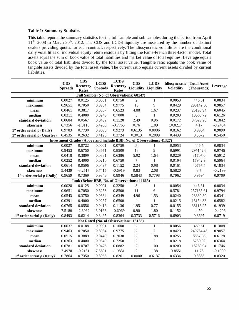
Table 1: Summary Statistics This table reports the summary statistics for the full sample and sub-samples during the period from April 11th, 2008 to March 30th, 2012. The CDS and LCDS liquidity are measured by the number of distinct dealers providing quotes for each contract, respectively. The idiosyncratic volatilities are the conditional daily volatilities of individual equity return residuals by fitting the Fama-French three-factor model. Total assets equal the sum of book value of total liabilities and market value of total equities. Leverage equals book value of total liabilities divided by the total asset value. Tangible ratio equals the book value of tangible assets divided by the total asset value. The current ratio equals current assets divided by current liabilities.
CDS
Spreads
CDS Recovery
Rates
LCDS Spreads
LCDS Recovery
Rates
CDS Liquidity
LCDS Liquidity
Idiosyncratic Volatility
Total Asset (Thousands) Leverage
Full Sample (No. of Observations: 68147) minimum 0.0027 0.0125 0.0001 0.0750 2 1 0.0053 446.51 0.0834 maximum 0.9651 0.7050 0.8984 0.9775 18 9 0.8429 295142.56 0.9857
mean 0.0461 0.3817 0.0367 0.6523 4.88 1.67 0.0237 25193.94 0.6045 median 0.0311 0.4000 0.0243 0.7000 5 1 0.0203 13565.72 0.6126
standard deviation 0.0684 0.0567 0.0482 0.1128 2.49 0.96 0.0172 37329.28 0.1842 skewness 6.7356 -1.8116 6.4265 -0.7765 0.76 1.89 10.8217 4.17 -0.2464
1st order serial ρ (Daily) 0.9783 0.7730 0.9690 0.9273 0.6135 0.8006 0.8162 0.9904 0.9890 1st order serial ρ (Quarter) 0.4535 0.2632 0.4125 0.3724 0.3013 0.2889 0.4439 0.5672 0.5450
Investment Grades (Above and include BBB, No. of Observations: 41327) minimum 0.0027 0.0722 0.0001 0.0750 3 1 0.0053 446.5 0.0834 maximum 0.9453 0.6750 0.8671 0.8500 18 9 0.6991 295142.6 0.9746
mean 0.0418 0.3809 0.0331 0.6386 5.92 1.64 0.0229 31707.0 0.5912 median 0.0252 0.4000 0.0210 0.6750 7 1 0.0194 17942.9 0.5964
standard deviation 0.0614 0.0506 0.0497 0.1152 2.24 0.98 0.0161 40757.4 0.1834 skewness 5.4439 -3.2517 6.7415 -0.6919 0.83 2.08 8.5820 3.7 -0.2199
1st order serial ρ (Daily) 0.9659 0.7369 0.9346 0.8946 0.5843 0.7798 0.7962 0.9594 0.9709 Junk (Below BBB, No. of Observations: 11665)
minimum 0.0028 0.0125 0.0001 0.3250 3 1 0.0054 446.51 0.0834 maximum 0.9651 0.7050 0.6253 0.8500 11 6 0.5781 257135.61 0.9794
mean 0.0543 0.3750 0.0384 0.6349 4.96 1.53 0.0240 23330.80 0.6341 median 0.0391 0.4000 0.0257 0.6500 4 1 0.0215 13154.38 0.6582
standard deviation 0.0765 0.0556 0.0416 0.1136 1.95 0.77 0.0155 38118.25 0.1939 skewness 7.5180 -2.3062 3.0163 -0.6069 0.90 1.80 8.1152 4.50 -0.4206
1st order serial ρ (Daily) 0.8493 0.6214 0.8495 0.8364 0.3733 0.5716 0.6903 0.8697 0.8719 Not Rated (No. of Observations: 15155)
minimum 0.0037 0.0188 0.0001 0.1000 2 1 0.0056 450.51 0.1008 maximum 0.9463 0.7050 0.8984 0.9775 2 7 0.8429 249734.43 0.9857
mean 0.0515 0.3889 0.0449 0.7030 2 1.88 0.0255 8867.08 0.6178 median 0.0363 0.4000 0.0349 0.7250 2 2 0.0218 5739.02 0.6364
standard deviation 0.0781 0.0707 0.0476 0.0882 2 1.00 0.0209 15260.94 0.1746 skewness 7.4978 -0.2131 7.5601 -1.0831 2 1.38 13.8551 11.73 -0.1909
1st order serial ρ (Daily) 0.7864 0.7350 0.8066 0.8261 0.0000 0.6137 0.6336 0.8855 0.8320
55
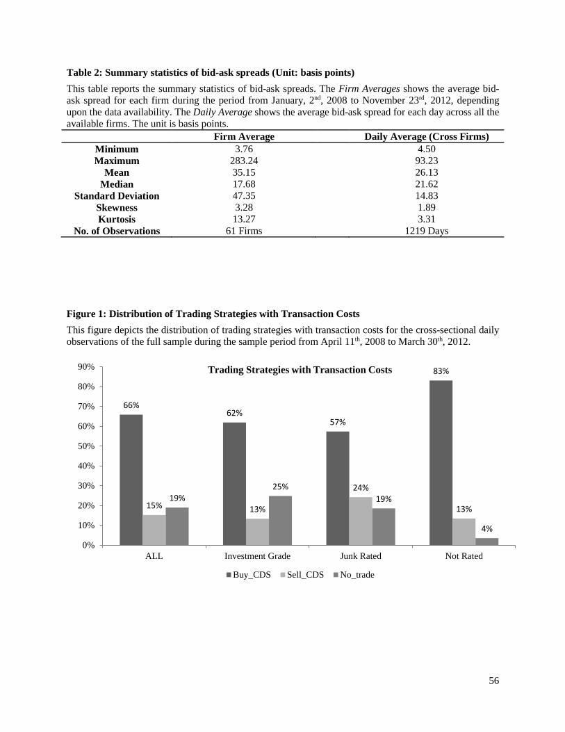
Table 2: Summary statistics of bid-ask spreads (Unit: basis points) This table reports the summary statistics of bid-ask spreads. The Firm Averages shows the average bid-ask spread for each firm during the period from January, 2nd, 2008 to November 23rd, 2012, depending upon the data availability. The Daily Average shows the average bid-ask spread for each day across all the available firms. The unit is basis points.
Firm Average Daily Average (Cross Firms) Minimum 3.76 4.50 Maximum 283.24 93.23
Mean 35.15 26.13 Median 17.68 21.62
Standard Deviation 47.35 14.83 Skewness 3.28 1.89 Kurtosis 13.27 3.31
No. of Observations 61 Firms 1219 Days
Figure 1: Distribution of Trading Strategies with Transaction Costs This figure depicts the distribution of trading strategies with transaction costs for the cross-sectional daily observations of the full sample during the sample period from April 11th, 2008 to March 30th, 2012.
66%62%
57%
83%
15% 13%
24%
13%19%
25%19%
4%
0%
10%
20%
30%
40%
50%
60%
70%
80%
90%
ALL Investment Grade Junk Rated Not Rated
Trading Strategies with Transaction Costs
Buy_CDS Sell_CDS No_trade
56
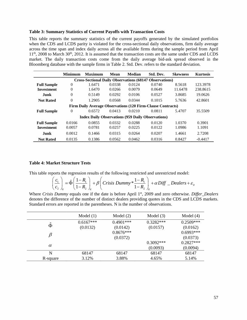
Table 3: Summary Statistics of Current Payoffs with Transaction Costs This table reports the summary statistics of the current payoffs generated by the simulated portfolios when the CDS and LCDS parity is violated for the cross-sectional daily observations, firm daily average across the time span and index daily across all the available firms during the sample period from April 11th, 2008 to March 30th, 2012. It is assumed that the transaction costs are the same under CDS and LCDS market. The daily transaction costs come from the daily average bid-ask spread observed in the Bloomberg database with the sample firms in Table 2. Std. Dev. refers to the standard deviation.
Minimum Maximum Mean Median Std. Dev. Skewness Kurtosis Cross-Sectional Daily Observations (68147 Observations)
Full Sample 0 1.6471 0.0338 0.0124 0.0740 8.5618 123.3978 Investment 0 1.6470 0.0266 0.0079 0.0649 11.6478 238.8615
Junk 0 0.5149 0.0292 0.0106 0.0527 3.8685 19.0626 Not Rated 0 1.2905 0.0568 0.0344 0.1015 5.7636 42.8601
Firm Daily Average Observations (120 Firm-Clause Contracts) Full Sample 0 0.6572 0.0413 0.0210 0.0811 5.4707 35.5509
Index Daily Observations (959 Daily Observations) Full Sample 0.0166 0.0855 0.0332 0.0288 0.0120 1.0370 0.3901 Investment 0.0057 0.0781 0.0257 0.0225 0.0122 1.0986 1.1091
Junk 0.0012 0.1466 0.0315 0.0264 0.0207 1.4661 2.7208 Not Rated 0.0135 0.1386 0.0562 0.0462 0.0316 0.8427 -0.4417
Table 4: Market Structure Tests This table reports the regression results of the following restricted and unrestricted model:
1 1 1
2 2 2
1 1ˆ * _1 1 it
it it it
c R RCrisis Dummy Diff Dealersc R R
β α ε − −
= Φ + + + − −
Where Crisis Dummy equals one if the date is before April 1st, 2009 and zero otherwise. Differ_Dealers denotes the difference of the number of distinct dealers providing quotes in the CDS and LCDS markets. Standard errors are reported in the parentheses. N is the number of observations.
Model (1) Model (2) Model (3) Model (4)
Φ 0.6167*** (0.0132)
0.4901*** (0.0142)
0.3282*** (0.0157)
0.2509*** (0.0162)
β 0.8676*** (0.0372) 0.6993***
(0.0373)
α 0.3092*** (0.0093)
0.2827*** (0.0094)
N 68147 68147 68147 68147 R-square 3.12% 3.88% 4.65% 5.14%
57
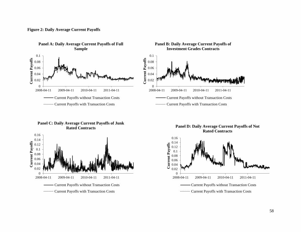
Figure 2: Daily Average Current Payoffs
0
0.02
0.04
0.06
0.08
0.1
2008-04-11 2009-04-11 2010-04-11 2011-04-11
Cur
rent
Pay
offs
Panel A: Daily Average Current Payoffs of Full Sample
Current Payoffs without Transaction Costs
Current Payoffs with Transaction Costs
0
0.02
0.04
0.06
0.08
0.1
2008-04-11 2009-04-11 2010-04-11 2011-04-11
Cur
rent
Pay
offs
Panel B: Daily Average Current Payoffs of Investment Grades Contracts
Current Payoffs without Transaction Costs
Current Payoffs with Transaction Costs
00.020.040.060.080.1
0.120.140.16
2008-04-11 2009-04-11 2010-04-11 2011-04-11
Cur
rent
Pay
offs
Panel C: Daily Average Current Payoffs of Junk Rated Contracts
Current Payoffs without Transaction Costs
Current Payoffs with Transaction Costs
00.020.040.060.080.1
0.120.140.16
2008-04-11 2009-04-11 2010-04-11 2011-04-11
Cur
rent
Pay
offs
Panel D: Daily Average Current Payoffs of Not Rated Contracts
Current Payoffs without Transaction Costs
Current Payoffs with Transaction Costs
58
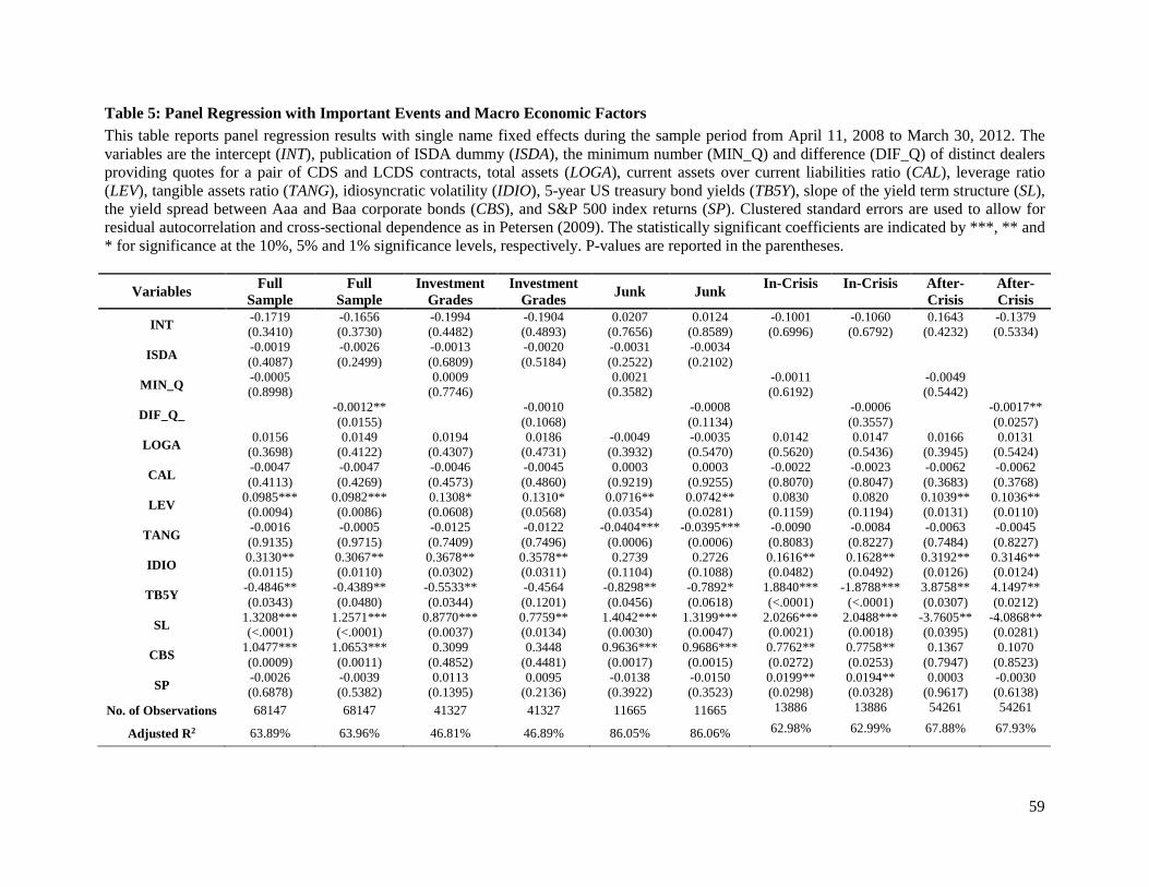
Table 5: Panel Regression with Important Events and Macro Economic Factors This table reports panel regression results with single name fixed effects during the sample period from April 11, 2008 to March 30, 2012. The variables are the intercept (INT), publication of ISDA dummy (ISDA), the minimum number (MIN_Q) and difference (DIF_Q) of distinct dealers providing quotes for a pair of CDS and LCDS contracts, total assets (LOGA), current assets over current liabilities ratio (CAL), leverage ratio (LEV), tangible assets ratio (TANG), idiosyncratic volatility (IDIO), 5-year US treasury bond yields (TB5Y), slope of the yield term structure (SL), the yield spread between Aaa and Baa corporate bonds (CBS), and S&P 500 index returns (SP). Clustered standard errors are used to allow for residual autocorrelation and cross-sectional dependence as in Petersen (2009). The statistically significant coefficients are indicated by ***, ** and * for significance at the 10%, 5% and 1% significance levels, respectively. P-values are reported in the parentheses.
Variables Full Sample
Full Sample
Investment Grades
Investment Grades Junk Junk In-Crisis In-Crisis After-
Crisis After-Crisis
INT -0.1719 (0.3410)
-0.1656 (0.3730)
-0.1994 (0.4482)
-0.1904 (0.4893)
0.0207 (0.7656)
0.0124 (0.8589)
-0.1001 (0.6996)
-0.1060 (0.6792)
0.1643 (0.4232)
-0.1379 (0.5334)
ISDA -0.0019 (0.4087)
-0.0026 (0.2499)
-0.0013 (0.6809)
-0.0020 (0.5184)
-0.0031 (0.2522)
-0.0034 (0.2102)
MIN_Q -0.0005 (0.8998) 0.0009
(0.7746) 0.0021 (0.3582) -0.0011
(0.6192) -0.0049
(0.5442)
DIF_Q_ -0.0012** (0.0155) -0.0010
(0.1068) -0.0008 (0.1134)
-0.0006 (0.3557)
-0.0017** (0.0257)
LOGA 0.0156 (0.3698)
0.0149 (0.4122)
0.0194 (0.4307)
0.0186 (0.4731)
-0.0049 (0.3932)
-0.0035 (0.5470)
0.0142 (0.5620)
0.0147 (0.5436)
0.0166 (0.3945)
0.0131 (0.5424)
CAL -0.0047 (0.4113)
-0.0047 (0.4269)
-0.0046 (0.4573)
-0.0045 (0.4860)
0.0003 (0.9219)
0.0003 (0.9255)
-0.0022 (0.8070)
-0.0023 (0.8047)
-0.0062 (0.3683)
-0.0062 (0.3768)
LEV 0.0985*** (0.0094)
0.0982*** (0.0086)
0.1308* (0.0608)
0.1310* (0.0568)
0.0716** (0.0354)
0.0742** (0.0281)
0.0830 (0.1159)
0.0820 (0.1194)
0.1039** (0.0131)
0.1036** (0.0110)
TANG -0.0016 (0.9135)
-0.0005 (0.9715)
-0.0125 (0.7409)
-0.0122 (0.7496)
-0.0404*** (0.0006)
-0.0395*** (0.0006)
-0.0090 (0.8083)
-0.0084 (0.8227)
-0.0063 (0.7484)
-0.0045 (0.8227)
IDIO 0.3130** (0.0115)
0.3067** (0.0110)
0.3678** (0.0302)
0.3578** (0.0311)
0.2739 (0.1104)
0.2726 (0.1088)
0.1616** (0.0482)
0.1628** (0.0492)
0.3192** (0.0126)
0.3146** (0.0124)
TB5Y -0.4846** (0.0343)
-0.4389** (0.0480)
-0.5533** (0.0344)
-0.4564 (0.1201)
-0.8298** (0.0456)
-0.7892* (0.0618)
1.8840*** (<.0001)
-1.8788*** (<.0001)
3.8758** (0.0307)
4.1497** (0.0212)
SL 1.3208*** (<.0001)
1.2571*** (<.0001)
0.8770*** (0.0037)
0.7759** (0.0134)
1.4042*** (0.0030)
1.3199*** (0.0047)
2.0266*** (0.0021)
2.0488*** (0.0018)
-3.7605** (0.0395)
-4.0868** (0.0281)
CBS 1.0477*** (0.0009)
1.0653*** (0.0011)
0.3099 (0.4852)
0.3448 (0.4481)
0.9636*** (0.0017)
0.9686*** (0.0015)
0.7762** (0.0272)
0.7758** (0.0253)
0.1367 (0.7947)
0.1070 (0.8523)
SP -0.0026 (0.6878)
-0.0039 (0.5382)
0.0113 (0.1395)
0.0095 (0.2136)
-0.0138 (0.3922)
-0.0150 (0.3523)
0.0199** (0.0298)
0.0194** (0.0328)
0.0003 (0.9617)
-0.0030 (0.6138)
No. of Observations 68147 68147 41327 41327 11665 11665 13886 13886 54261 54261
Adjusted R2 63.89% 63.96% 46.81% 46.89% 86.05% 86.06% 62.98% 62.99% 67.88% 67.93%
59
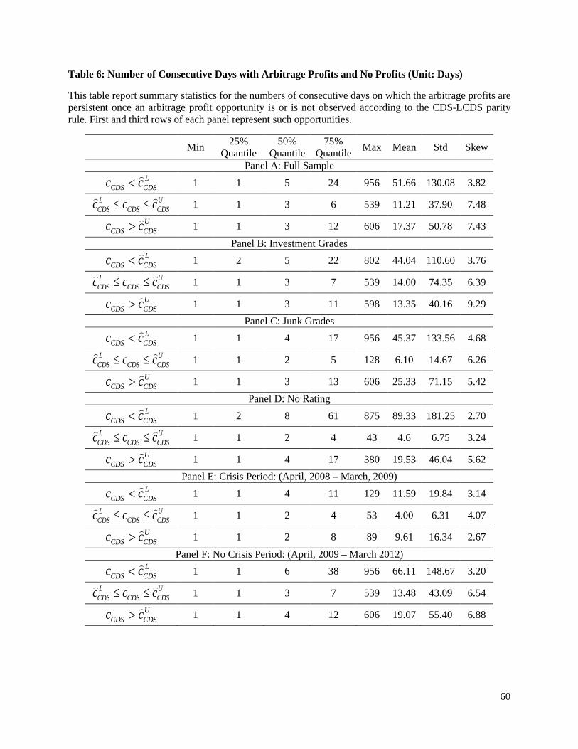
Table 6: Number of Consecutive Days with Arbitrage Profits and No Profits (Unit: Days)
This table report summary statistics for the numbers of consecutive days on which the arbitrage profits are persistent once an arbitrage profit opportunity is or is not observed according to the CDS-LCDS parity rule. First and third rows of each panel represent such opportunities.
Min 25% Quantile
50% Quantile
75% Quantile Max Mean Std Skew
Panel A: Full Sample L
CDS CDSc c< 1 1 5 24 956 51.66 130.08 3.82 L U
CDS CDS CDSc c c≤ ≤
1 1 3 6 539 11.21 37.90 7.48 U
CDS CDSc c> 1 1 3 12 606 17.37 50.78 7.43 Panel B: Investment Grades
LCDS CDSc c< 1 2 5 22 802 44.04 110.60 3.76
L UCDS CDS CDSc c c≤ ≤
1 1 3 7 539 14.00 74.35 6.39 U
CDS CDSc c> 1 1 3 11 598 13.35 40.16 9.29 Panel C: Junk Grades
LCDS CDSc c< 1 1 4 17 956 45.37 133.56 4.68
L UCDS CDS CDSc c c≤ ≤
1 1 2 5 128 6.10 14.67 6.26 U
CDS CDSc c> 1 1 3 13 606 25.33 71.15 5.42 Panel D: No Rating
LCDS CDSc c< 1 2 8 61 875 89.33 181.25 2.70
L UCDS CDS CDSc c c≤ ≤
1 1 2 4 43 4.6 6.75 3.24 U
CDS CDSc c> 1 1 4 17 380 19.53 46.04 5.62 Panel E: Crisis Period: (April, 2008 – March, 2009)
LCDS CDSc c< 1 1 4 11 129 11.59 19.84 3.14
L UCDS CDS CDSc c c≤ ≤
1 1 2 4 53 4.00 6.31 4.07 U
CDS CDSc c> 1 1 2 8 89 9.61 16.34 2.67 Panel F: No Crisis Period: (April, 2009 – March 2012)
LCDS CDSc c< 1 1 6 38 956 66.11 148.67 3.20
L UCDS CDS CDSc c c≤ ≤
1 1 3 7 539 13.48 43.09 6.54 U
CDS CDSc c> 1 1 4 12 606 19.07 55.40 6.88
60
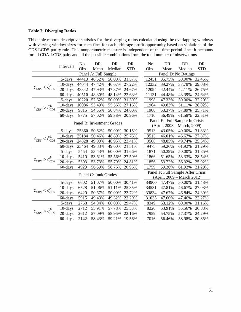
Table 7: Diverging Ratios
This table reports descriptive statistics for the diverging ratios calculated using the overlapping windows with varying window sizes for each firm for each arbitrage profit opportunity based on violations of the CDS-LCDS parity rule. This nonparametric measure is independent of the time period since it accounts for all CDA-LCDS pairs and all the possible combinations from the total number of observations.
Intervals No. Obs
DR Mean
DR Median
DR STD
No. Obs
DR Mean
DR Median
DR STD
Panel A: Full Sample Panel D: No Ratings
LCDS CDSc c<
5-days 44413 46.52% 50.00% 31.57% 12451 35.75% 30.00% 32.45% 10-days 44044 47.42% 46.67% 27.22% 12332 39.27% 37.78% 29.08% 20-days 43342 47.93% 47.37% 24.67% 12094 42.44% 42.11% 26.75% 60-days 40510 48.30% 48.14% 22.63% 11131 44.48% 43.39% 24.64%
UCDS CDSc c>
5-days 10220 52.62% 50.00% 31.30% 1998 47.33% 50.00% 32.20% 10-days 10086 53.49% 55.56% 27.16% 1964 49.83% 51.11% 28.02% 20-days 9815 54.55% 56.84% 24.60% 1900 53.37% 57.89% 25.71% 60-days 8775 57.02% 59.38% 20.96% 1710 56.49% 61.58% 22.51%
Panel B: Investment Grades Panel E: Full Sample In Crisis (April, 2008 – March, 2009)
LCDS CDSc c<
5-days 25360 50.62% 50.00% 30.15% 9513 43.05% 40.00% 31.83% 10-days 25184 50.46% 48.89% 25.76% 9513 46.01% 46.67% 27.87% 20-days 24828 49.90% 48.95% 23.41% 9508 48.85% 49.74% 25.64% 60-days 23464 49.83% 49.60% 21.51% 9475 59.26% 61.92% 21.29%
UCDS CDSc c>
5-days 5454 53.43% 60.00% 31.66% 1871 50.39% 50.00% 31.85% 10-days 5410 53.61% 55.56% 27.59% 1866 51.65% 53.33% 28.54% 20-days 5303 53.73% 55.79% 24.81% 1856 53.72% 56.32% 25.92% 60-days 4923 56.59% 58.76% 20.96% 1759 59.26% 61.92% 21.29%
Panel C: Junk Grades Panel F: Full Sample After Crisis (April, 2009 – March 2012)
LCDS CDSc c<
5-days 6602 51.07% 50.00% 30.41% 34900 47.47% 50.00% 31.43% 10-days 6528 51.06% 51.11% 25.85% 34531 47.81% 46.67% 27.03% 20-days 6420 50.67% 50.00% 23.72% 33834 47.67% 46.84% 24.39% 60-days 5915 49.43% 49.32% 22.20% 31035 47.66% 47.46% 22.27%
UCDS CDSc c>
5-days 2768 54.84% 60.00% 29.47% 8349 53.12% 60.00% 31.16% 10-days 2712 55.91% 57.78% 25.33% 8220 53.91% 55.56% 26.83% 20-days 2612 57.09% 58.95% 23.16% 7959 54.75% 57.37% 24.29% 60-days 2142 58.43% 59.21% 19.56% 7016 56.46% 58.98% 20.85%
61
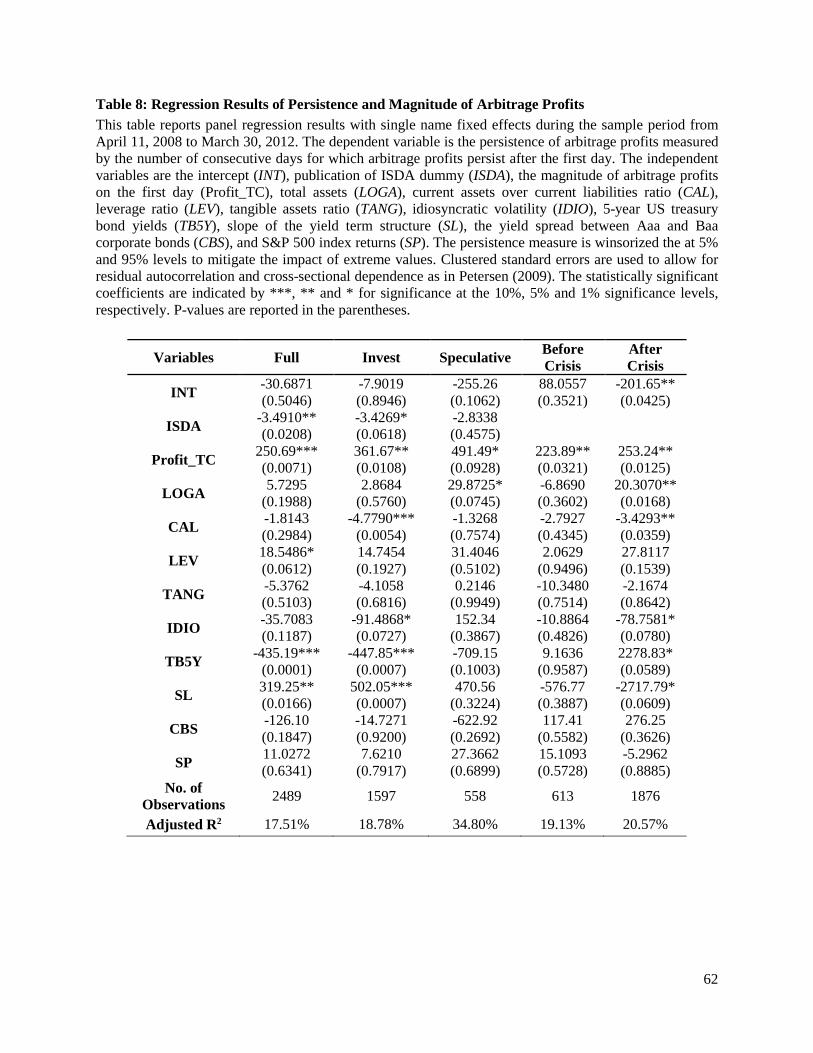
Table 8: Regression Results of Persistence and Magnitude of Arbitrage Profits This table reports panel regression results with single name fixed effects during the sample period from April 11, 2008 to March 30, 2012. The dependent variable is the persistence of arbitrage profits measured by the number of consecutive days for which arbitrage profits persist after the first day. The independent variables are the intercept (INT), publication of ISDA dummy (ISDA), the magnitude of arbitrage profits on the first day (Profit_TC), total assets (LOGA), current assets over current liabilities ratio (CAL), leverage ratio (LEV), tangible assets ratio (TANG), idiosyncratic volatility (IDIO), 5-year US treasury bond yields (TB5Y), slope of the yield term structure (SL), the yield spread between Aaa and Baa corporate bonds (CBS), and S&P 500 index returns (SP). The persistence measure is winsorized the at 5% and 95% levels to mitigate the impact of extreme values. Clustered standard errors are used to allow for residual autocorrelation and cross-sectional dependence as in Petersen (2009). The statistically significant coefficients are indicated by ***, ** and * for significance at the 10%, 5% and 1% significance levels, respectively. P-values are reported in the parentheses.
Variables Full Invest Speculative Before Crisis
After Crisis
INT -30.6871 (0.5046)
-7.9019 (0.8946)
-255.26 (0.1062)
88.0557 (0.3521)
-201.65** (0.0425)
ISDA -3.4910** (0.0208)
-3.4269* (0.0618)
-2.8338 (0.4575)
Profit_TC 250.69*** (0.0071)
361.67** (0.0108)
491.49* (0.0928)
223.89** (0.0321)
253.24** (0.0125)
LOGA 5.7295 (0.1988)
2.8684 (0.5760)
29.8725* (0.0745)
-6.8690 (0.3602)
20.3070** (0.0168)
CAL -1.8143 (0.2984)
-4.7790*** (0.0054)
-1.3268 (0.7574)
-2.7927 (0.4345)
-3.4293** (0.0359)
LEV 18.5486* (0.0612)
14.7454 (0.1927)
31.4046 (0.5102)
2.0629 (0.9496)
27.8117 (0.1539)
TANG -5.3762 (0.5103)
-4.1058 (0.6816)
0.2146 (0.9949)
-10.3480 (0.7514)
-2.1674 (0.8642)
IDIO -35.7083 (0.1187)
-91.4868* (0.0727)
152.34 (0.3867)
-10.8864 (0.4826)
-78.7581* (0.0780)
TB5Y -435.19*** (0.0001)
-447.85*** (0.0007)
-709.15 (0.1003)
9.1636 (0.9587)
2278.83* (0.0589)
SL 319.25** (0.0166)
502.05*** (0.0007)
470.56 (0.3224)
-576.77 (0.3887)
-2717.79* (0.0609)
CBS -126.10 (0.1847)
-14.7271 (0.9200)
-622.92 (0.2692)
117.41 (0.5582)
276.25 (0.3626)
SP 11.0272 (0.6341)
7.6210 (0.7917)
27.3662 (0.6899)
15.1093 (0.5728)
-5.2962 (0.8885)
No. of Observations 2489 1597 558 613 1876
Adjusted R2 17.51% 18.78% 34.80% 19.13% 20.57%
62
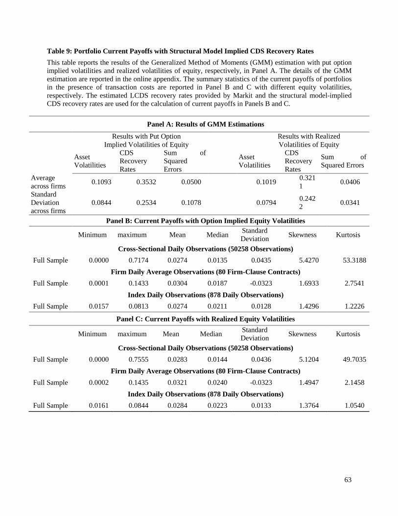
Table 9: Portfolio Current Payoffs with Structural Model Implied CDS Recovery Rates This table reports the results of the Generalized Method of Moments (GMM) estimation with put option implied volatilities and realized volatilities of equity, respectively, in Panel A. The details of the GMM estimation are reported in the online appendix. The summary statistics of the current payoffs of portfolios in the presence of transaction costs are reported in Panel B and C with different equity volatilities, respectively. The estimated LCDS recovery rates provided by Markit and the structural model-implied CDS recovery rates are used for the calculation of current payoffs in Panels B and C.
Panel A: Results of GMM Estimations
Results with Put Option Implied Volatilities of Equity Results with Realized
Volatilities of Equity
Asset Volatilities
CDS Recovery Rates
Sum of Squared Errors
Asset Volatilities
CDS Recovery Rates
Sum of Squared Errors
Average across firms 0.1093 0.3532 0.0500 0.1019 0.321
1 0.0406
Standard Deviation across firms
0.0844 0.2534 0.1078 0.0794 0.2422 0.0341
Panel B: Current Payoffs with Option Implied Equity Volatilities
Minimum maximum Mean Median Standard Deviation Skewness Kurtosis
Cross-Sectional Daily Observations (50258 Observations) Full Sample 0.0000 0.7174 0.0274 0.0135 0.0435 5.4270 53.3188
Firm Daily Average Observations (80 Firm-Clause Contracts) Full Sample 0.0001 0.1433 0.0304 0.0187 -0.0323 1.6933 2.7541
Index Daily Observations (878 Daily Observations) Full Sample 0.0157 0.0813 0.0274 0.0211 0.0128 1.4296 1.2226
Panel C: Current Payoffs with Realized Equity Volatilities
Minimum maximum Mean Median Standard Deviation Skewness Kurtosis
Cross-Sectional Daily Observations (50258 Observations) Full Sample 0.0000 0.7555 0.0283 0.0144 0.0436 5.1204 49.7035
Firm Daily Average Observations (80 Firm-Clause Contracts) Full Sample 0.0002 0.1435 0.0321 0.0240 -0.0323 1.4947 2.1458
Index Daily Observations (878 Daily Observations) Full Sample 0.0161 0.0844 0.0284 0.0223 0.0133 1.3764 1.0540
63
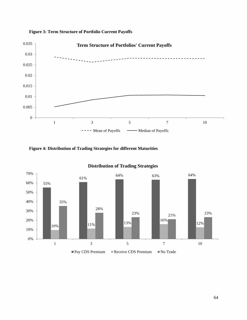
Figure 3: Term Structure of Portfolio Current Payoffs
Figure 4: Distribution of Trading Strategies for different Maturities
0
0.005
0.01
0.015
0.02
0.025
0.03
0.035
1 3 5 7 10
Term Structure of Portfolios' Current Payoffs
Mean of Payoffs Median of Payoffs
55%61%
64% 63% 64%
10% 11% 13%16%
12%
35%
28%23% 21% 23%
0%
10%
20%
30%
40%
50%
60%
70%
1 3 5 7 10
Distribution of Trading Strategies
Pay CDS Premium Receive CDS Premium No Trade
64
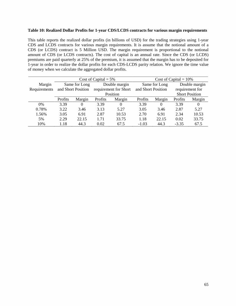
Table 10: Realized Dollar Profits for 1-year CDS/LCDS contracts for various margin requirements This table reports the realized dollar profits (in billions of USD) for the trading strategies using 1-year CDS and LCDS contracts for various margin requirements. It is assume that the notional amount of a CDS (or LCDS) contract is 5 Million USD. The margin requirement is proportional to the notional amount of CDS (or LCDS contracts). The cost of capital is an annual rate. Since the CDS (or LCDS) premiums are paid quarterly at 25% of the premium, it is assumed that the margin has to be deposited for 1-year in order to realize the dollar profits for each CDS-LCDS parity relation. We ignore the time value of money when we calculate the aggregated dollar profits.
Cost of Capital = 5% Cost of Capital = 10% Margin
Requirements Same for Long
and Short Position Double margin
requirement for Short Position
Same for Long and Short Position
Double margin requirement for Short Position
Profits Margin Profits Margin Profits Margin Profits Margin 0% 3.39 0 3.39 0 3.39 0 3.39 0
0.78% 3.22 3.46 3.13 5.27 3.05 3.46 2.87 5.27 1.56% 3.05 6.91 2.87 10.53 2.70 6.91 2.34 10.53
5% 2.29 22.15 1.71 33.75 1.18 22.15 0.02 33.75 10% 1.18 44.3 0.02 67.5 -1.03 44.3 -3.35 67.5
65
Top Related