

![A Mean Field View of the Landscape of Two-Layers Neural … · 2018. 6. 6. · AMeanFieldViewoftheLandscape ofTwo-LayersNeuralNetworks AndreaMontanari [withSongMei,Phan-MinhNguyen]](https://static.fdocument.pub/doc/165x107/611227ff8db59724b615a22f/a-mean-field-view-of-the-landscape-of-two-layers-neural-2018-6-6-ameanfieldviewofthelandscape.jpg)


![Adaptive Consensus of Discrete-time Heterogeneous Multi ... · Multi-Agent Dynamical Systems (MADSs) 2 SICE Annual Conference 2011 2011/9/16 Active research field [Fax & Murray 2004]](https://static.fdocument.pub/doc/165x107/60114304fea62a4de827be08/adaptive-consensus-of-discrete-time-heterogeneous-multi-multi-agent-dynamical.jpg)


Languages
Pages
Legal

KH Computational Physics- 2010 QMC
Dynamical Mean Field Theory +Band Structure Method
1 GW+DMFT
We will express the various types of approximations in language of Luttinger-Ward
functionals.
The exact Luttinger Ward functional takes the form
Γ[G] = Tr log G − Tr(ΣG) + Φ[G] (1)
where Φ[G] is the sum of all possible two particle irreducible skeleton diagrams obtained
by the bare Coulomb interaction VC(r − r′) = 1
|r−r′| and the fully dressed propagator
G(r, r′).
We notice the following
Kristjan Haule, 2010 –1–
KH Computational Physics- 2010 QMC
• When bands are very wide, the kinetic energy is much bigger then the potential energy.
The perturbation theory in Coulomb interaction VC is converging rapidly and band
structure methods, such as LDA or GW are very accurate. Typical examples are noble
metals (Cu, Ag, Au).
• In narrow band materials, such as transition metals, transition metal oxides,
intermetallic f materials,... the potential energy is large compared to kinetic energy.
The band structure methods such as LDA or GW perform much worse. They
dramatically brake down in Mott insulators.
• In correlated materials, all higher order Feynman graps are important.
• The higher order graps are very local (only Hartree-Fock graph is nonlocal in infinite D
when interaction is non-local), and could be summed by the DMFT method.
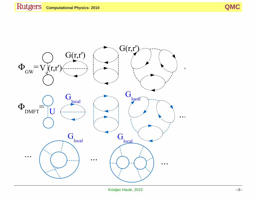
Let’s first explain the idea of GW+DMFT, because GW is diagrammatic method, and there
is no ambiguity in defining GW+DMFT. The Φ functionals of the two method, GW and
DMFT are
Kristjan Haule, 2010 –2–
KH Computational Physics- 2010 QMC
Kristjan Haule, 2010 –3–
KH Computational Physics- 2010 QMC
The GW method sums all RPA-like diagrams, but the propagator is the fully interacting
Green’s function G−1(r, r′) = G−10 (r, r′) − ΣGW (r, r′). Here
G−10 = δ(r− r
′)(ω + µ +∇2 − Vext(r)) and ΣGW (r, r′) is the correction due to the
Coulomb interaction. The GW diagrams are plotted in black in the above figure.
The DMFT method sums all local digrams, regarding of their topology or order. The number
of diagrams is increasing exponentially with order, and we can not plot them even at modest
orders. All these diagrams are large in correlated materials. Since the high order diagrams
are much more local then the diagrams at low orders, it makes sense to combine the two
methods GW and DMFT into GW+DMFT. The Luttinger Ward functional is
ΦGW+DMFT = ΦGW (G(r, r′)) + ΦDMFT (Gloc) − ΦGW (Gloc) (2)
Becase the GW-type of the diagrams appear in both GW and DMFT the local GW diagrams
need to be subtracted.
We have thus defined the GW+DMFT approximation:
Γ[G(r, r′)] = Tr log G − Tr(ΣG) + ΦGW [G(r, r′)] + ΦDMFT [Gloc] − ΦGW [Gloc]. (3)
Kristjan Haule, 2010 –4–
KH Computational Physics- 2010 QMC
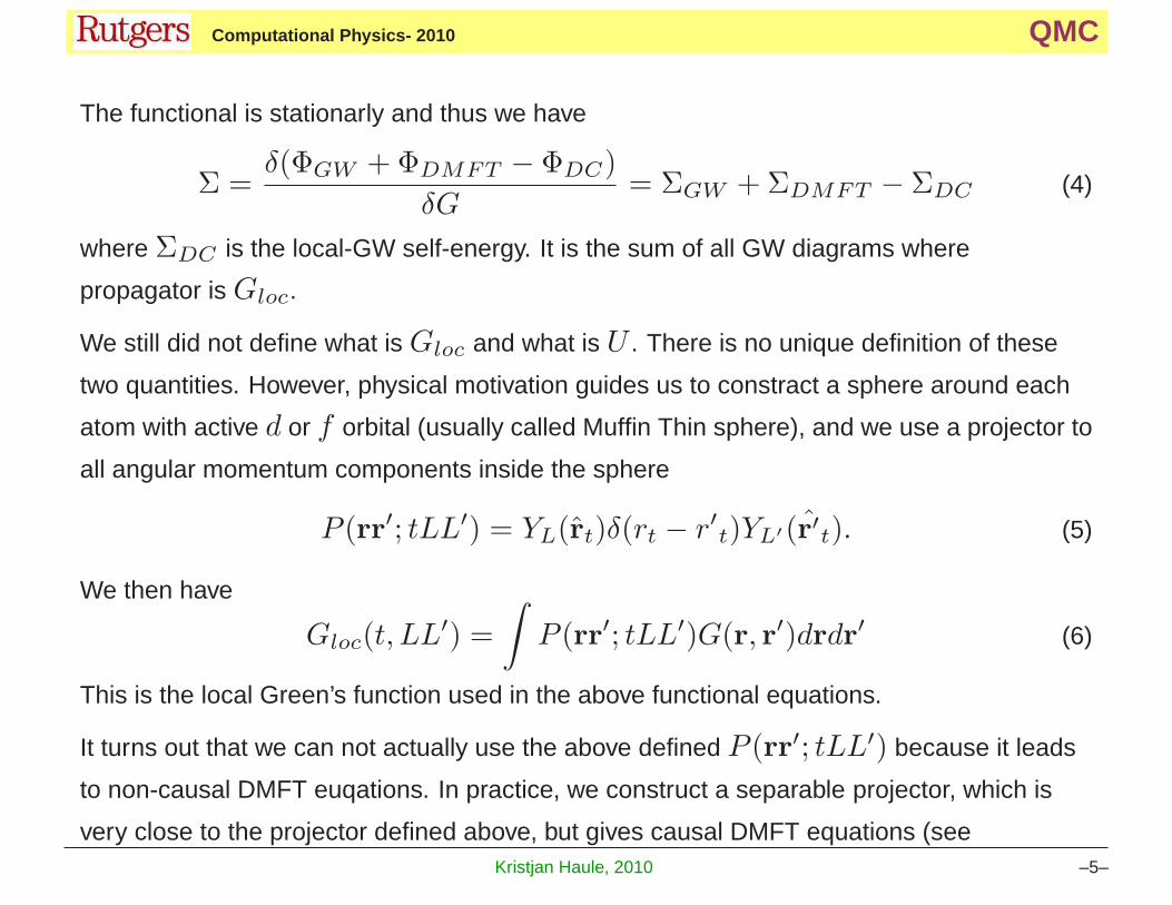
The functional is stationarly and thus we have
Σ =δ(ΦGW + ΦDMFT − ΦDC)
δG= ΣGW + ΣDMFT − ΣDC (4)
where ΣDC is the local-GW self-energy. It is the sum of all GW diagrams where
propagator is Gloc.
We still did not define what is Gloc and what is U . There is no unique definition of these
two quantities. However, physical motivation guides us to constract a sphere around each
atom with active d or f orbital (usually called Muffin Thin sphere), and we use a projector to
all angular momentum components inside the sphere
P (rr′; tLL′) = YL(r̂t)δ(rt − r′t)YL′(r̂′t). (5)
We then have
Gloc(t, LL′) =
∫P (rr′; tLL′)G(r, r′)drdr′ (6)
This is the local Green’s function used in the above functional equations.
It turns out that we can not actually use the above defined P (rr′; tLL′) because it leads
to non-causal DMFT euqations. In practice, we construct a separable projector, which is
very close to the projector defined above, but gives causal DMFT equations (seeKristjan Haule, 2010 –5–
KH Computational Physics- 2010 QMC
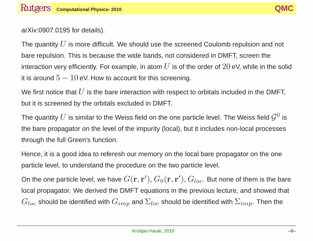
arXiv:0907.0195 for details).
The quantity U is more difficult. We should use the screened Coulomb repulsion and not
bare repulsion. This is because the wide bands, not considered in DMFT, screen the
interaction very efficiently. For example, in atom U is of the order of 20 eV, while in the solid
it is around 5 − 10 eV. How to account for this screening.
We first notice that U is the bare interaction with respect to orbitals included in the DMFT,
but it is screened by the orbitals excluded in DMFT.
The quantity U is similar to the Weiss field on the one particle level. The Weiss field G0 is
the bare propagator on the level of the impurity (local), but it includes non-local processes
through the full Green’s function.
Hence, it is a good idea to referesh our memory on the local bare propagator on the one
particle level, to understand the procedure on the two particle level.
On the one particle level, we have G(r, r′), G0(r, r′), Gloc. But none of them is the bare
local propagator. We derived the DMFT equations in the previous lecture, and showed that
Gloc should be identified with Gimp and Σloc should be identified with Σimp. Then the
Kristjan Haule, 2010 –6–
KH Computational Physics- 2010 QMC
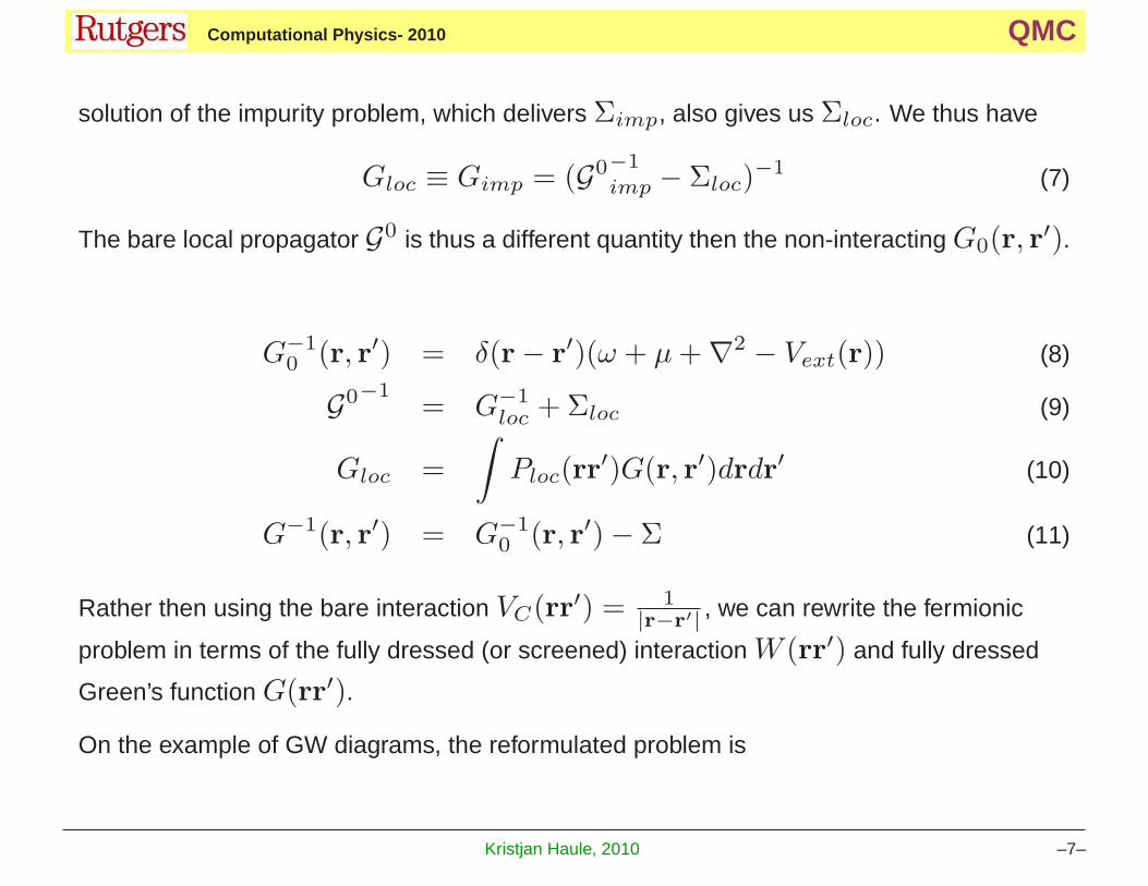
solution of the impurity problem, which delivers Σimp, also gives us Σloc. We thus have
Gloc ≡ Gimp = (G0−1
imp − Σloc)−1 (7)
The bare local propagator G0 is thus a different quantity then the non-interacting G0(r, r′).
G−10 (r, r′) = δ(r − r
′)(ω + µ + ∇2 − Vext(r)) (8)
G0−1= G−1
loc + Σloc (9)
Gloc =
∫Ploc(rr
′)G(r, r′)drdr′ (10)
G−1(r, r′) = G−10 (r, r′) − Σ (11)
Rather then using the bare interaction VC(rr′) = 1|r−r
′| , we can rewrite the fermionic
problem in terms of the fully dressed (or screened) interaction W (rr′) and fully dressed
Green’s function G(rr′).
On the example of GW diagrams, the reformulated problem is
Kristjan Haule, 2010 –7–

KH Computational Physics- 2010 QMC
Kristjan Haule, 2010 –8–

KH Computational Physics- 2010 QMC
Clearly, the screened interaction also obeys the Dyson equation
W−1(rr′) = V −1(rr′) − Π(rr′) (12)
where Π(rr′) is the polarizability. In GW, this is just the bubble.
We thus have a set of parallel quantities on the one and the two particle level
name one-particle two particle
bare propagator G0(rr′) Vc(rr
′) = 1|r−r
′|
fully dressed propagator G(rr′) W (rr′)
self-energy/polarizability Σ(rr′) Π(rr′)
local propagator Gloc Wloc
Weiss-field/screened interaction G0 U
On the two particle level, U is like the bare local propagator G0 on the one particle level,
and G0(r, r′) on the one particle level is like the bare Coulomb interaction 1/|r − r
′| on
the two particle level.
Kristjan Haule, 2010 –9–
KH Computational Physics- 2010 QMC
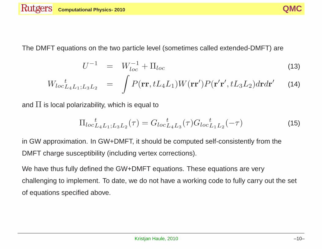
The DMFT equations on the two particle level (sometimes called extended-DMFT) are
U−1 = W−1loc + Πloc (13)
WloctL4L1;L3L2
=
∫P (rr, tL4L1)W (rr′)P (r′r′, tL3L2)drdr
′ (14)
and Π is local polarizability, which is equal to
ΠloctL4L1;L3L2
(τ) = GloctL4L3
(τ)GloctL1L2
(−τ) (15)
in GW approximation. In GW+DMFT, it should be computed self-consistently from the
DMFT charge susceptibility (including vertex corrections).
We have thus fully defined the GW+DMFT equations. These equations are very
challenging to implement. To date, we do not have a working code to fully carry out the set
of equations specified above.
Kristjan Haule, 2010 –10–
KH Computational Physics- 2010 QMC
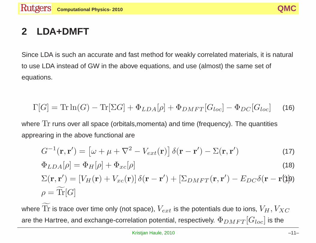
2 LDA+DMFT
Since LDA is such an accurate and fast method for weakly correlated materials, it is natural
to use LDA instead of GW in the above equations, and use (almost) the same set of
equations.
Γ[G] = Tr ln(G) − Tr[ΣG] + ΦLDA[ρ] + ΦDMFT [Gloc] − ΦDC [Gloc] (16)
where Tr runs over all space (orbitals,momenta) and time (frequency). The quantities
apprearing in the above functional are
G−1(r, r′) =[ω + µ + ∇2 − Vext(r)
]δ(r − r
′) − Σ(r, r′) (17)
ΦLDA[ρ] = ΦH [ρ] + Φxc[ρ] (18)
Σ(r, r′) = [VH(r) + Vxc(r)] δ(r − r′) + [ΣDMFT (r, r′) − EDCδ(r − r
′)](19)
ρ = T̃r[G]
where T̃r is trace over time only (not space), Vext is the potentials due to ions, VH , VXC
are the Hartree, and exchange-correlation potential, respectively. ΦDMFT [Gloc] is the
Kristjan Haule, 2010 –11–
KH Computational Physics- 2010 QMC
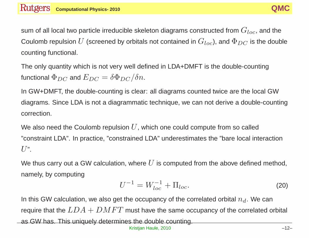
sum of all local two particle irreducible skeleton diagrams constructed from Gloc, and the
Coulomb repulsion U (screened by orbitals not contained in Gloc), and ΦDC is the double
counting functional.
The only quantity which is not very well defined in LDA+DMFT is the double-counting
functional ΦDC and EDC = δΦDC/δn.
In GW+DMFT, the double-counting is clear: all diagrams counted twice are the local GW
diagrams. Since LDA is not a diagrammatic technique, we can not derive a double-counting
correction.
We also need the Coulomb repulsion U , which one could compute from so called
”constraint LDA”. In practice, ”constrained LDA” underestimates the ”bare local interaction
U ”.
We thus carry out a GW calculation, where U is computed from the above defined method,
namely, by computing
U−1 = W−1loc + Πloc. (20)
In this GW calculation, we also get the occupancy of the correlated orbital nd. We can
require that the LDA + DMFT must have the same occupancy of the correlated orbital
as GW has. This uniquely determines the double counting.Kristjan Haule, 2010 –12–
KH Computational Physics- 2010 QMC
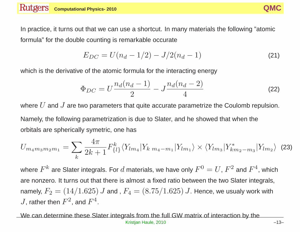
In practice, it turns out that we can use a shortcut. In many materials the following ”atomic
formula” for the double counting is remarkable occurate
EDC = U(nd − 1/2) − J/2(nd − 1) (21)
which is the derivative of the atomic formula for the interacting energy
ΦDC = Und(nd − 1)
2− J
nd(nd − 2)
4(22)
where U and J are two parameters that quite accurate parametrize the Coulomb repulsion.
Namely, the following parametrization is due to Slater, and he showed that when the
orbitals are spherically symetric, one has
Um4m3m2m1=
∑
k
4π
2k + 1F k{l}〈Ylm4
|Yk m4−m1|Ylm1
〉 × 〈Ylm3|Y ∗
km2−m3|Ylm2
〉 (23)
where F k are Slater integrals. For d materials, we have only F 0 = U , F 2 and F 4, which
are nonzero. It turns out that there is almost a fixed ratio between the two Slater integrals,
namely, F2 = (14/1.625) J and , F4 = (8.75/1.625) J . Hence, we usualy work with
J , rather then F 2, and F 4.
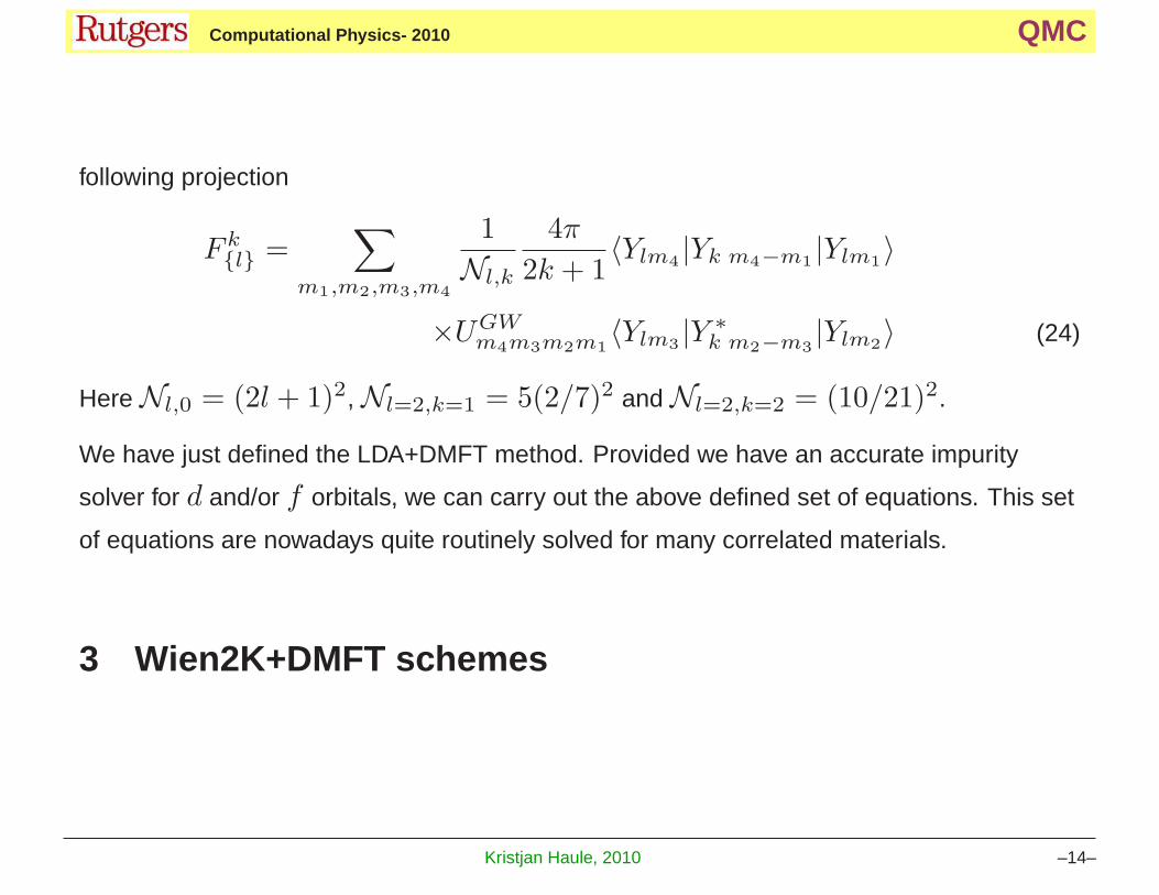
We can determine these Slater integrals from the full GW matrix of interaction by theKristjan Haule, 2010 –13–
KH Computational Physics- 2010 QMC
following projection
F k{l} =
∑
m1,m2,m3,m4
1
Nl,k
4π
2k + 1〈Ylm4
|Yk m4−m1|Ylm1
〉
×UGWm4m3m2m1
〈Ylm3|Y ∗
k m2−m3|Ylm2
〉 (24)
Here Nl,0 = (2l + 1)2, Nl=2,k=1 = 5(2/7)2 and Nl=2,k=2 = (10/21)2.
We have just defined the LDA+DMFT method. Provided we have an accurate impurity
solver for d and/or f orbitals, we can carry out the above defined set of equations. This set
of equations are nowadays quite routinely solved for many correlated materials.
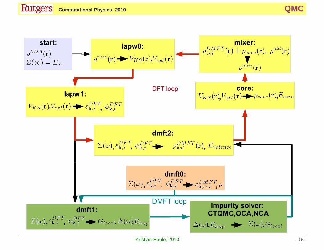
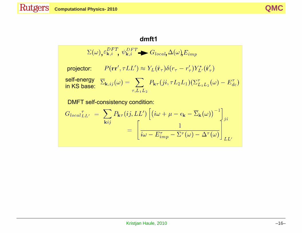
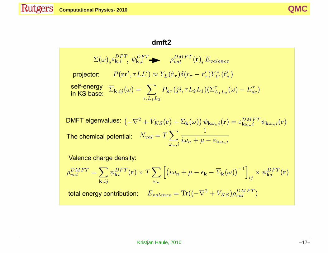
3 Wien2K+DMFT schemes
Kristjan Haule, 2010 –14–
KH Computational Physics- 2010 QMC
Kristjan Haule, 2010 –15–
KH Computational Physics- 2010 QMC
Kristjan Haule, 2010 –16–
KH Computational Physics- 2010 QMC
Kristjan Haule, 2010 –17–
Top Related