


Languages
Pages
Legal


8/18/2019 API RP 2P RP
http://slidepdf.com/reader/full/api-rp-2p-rp 1/68

8/18/2019 API RP 2P RP
http://slidepdf.com/reader/full/api-rp-2p-rp 2/68

8/18/2019 API RP 2P RP
http://slidepdf.com/reader/full/api-rp-2p-rp 3/68
makes no representation, warranty or guarantee in connection with the publication of this
Recommended Practice and hereby expressly disclaims any liability or responsibility for loss or
damage resulting from its use, for any violation of any federal, state or municipal regulation with which
an API recommendation may conflict, or for the infringement of any patent resulting from the use of this
publication.
NOTE: This recommended practice is under the jurisdiction of the API Committee on Standardization
of Offshore Structures. This is the second edition of this recommended practice and supersedes the
first edition dated Jan. 1, 1984. It was authorized for publication at the 1986 Standardization
Conference and later ratified by letter ballot.
Requests for permission to reproduce or translate all or any part of the material published herein should
be addressed to the Director, Production Department, 211 N. Ervay, Suite 1700, Dallas TX 75201.
SECTION 1 BASIC CONSIDERATIONS AND DATA REQUIREMENTS
1.1 Basic Considerations.
Drilling operations require that horizontal displacement of the drilling vessel be restricted within a
small radius of the wellbore centerline, primarily to protect the riser and the lower ball joint. The
allowable vessel displacement from the wellbore should be determined by analysis of the drilling riser.
Procedures described in API RP 2Q. "Design and Operation of Marine Drilling Riser Systems," should
be used to determine allowable offsets for the drilling vessel. Generally speaking, the drilling vesselshould be maintained within a watch circle with radius in the range of 3 to 6 percent of water depth
when drilling is proceeding. This radius can be increased to 8 to 10 percent of water depth when
drilling is suspended and the drilling riser is still connected to the seafloor. Should the riser be
disconnected from the seafloor, there is no restriction on the size of the watch circle.
The analysis method presented assumes that all equipment is either new or in a like-new condition
and has not been subjected to loading which would affect its fatigue life. The proper maintenance and
careful inspection of all equipment is strongly encouraged. The recommended design procedure
presupposes that winches, wildcats, fairleaders, pendants, buoys, etc., are also properly sized and in
good working order.
Mooring systems should be properly deployed. Competent personnel with proper equipment should be
utilized. Instrumentation for determining the amount of line out, tension in the lines, exact location of
anchor drop points, etc., can be very valuable during the deployment of a mooring system. As part of
the process of installing a mooring system, the mooring lines should be routinely tested. Mooring
lines should be tensioned to values which represent the maximum expected value for the particular
location. Lines which do not achieve this value should be reset and if necessary additional anchoring
equipment should be added.
[RP 2P] Copyright by American Petroleum Institute (Fri Jul 13 11:52:55 2001)

8/18/2019 API RP 2P RP
http://slidepdf.com/reader/full/api-rp-2p-rp 4/68
1.2 Purpose of Mooring Analysis.
A floating drilling vessel held on location with a spread mooring is shown in Figure 1. When wind,
current and waves act on the vessel, the total environmental force (F) pushes the rig a distance (x)
away from its initial position over the hole. The vessel comes to an equilibrium position when the
mooring develops a net restoring force equal to the steady-state environmental force.
As shown in Figure 1, wind, waves, and current induce movement of the vessel away from the
wellbore and increase the tension in the windward mooring lines while decreasing tension in the
leeward lines. Each mooring should be analyzed to ensure that developed tension (Tmax
) does not
exceed the maximum safe working load and that the load placed on the anchor (Amax
) does not
exceed its holding power. The holding power of an anchor is significantly reduced when the anchor is
subjected to a vertical load. To completely avoid vertical loads, the length of mooring line outboard of
the fairlead (Lmax
) must be long enough to allow the line to remain tangent to the sea bottom at the
anchor during periods of the highest expected line tensions. Also, the vessel movements should be
kept within certain limits that can be tolerated by the drilling riser.
A mooring analysis is often performed in conjunction with a riser analysis to determine:
• Limiting environments for operating and survival conditions
• Recommended mooring pattern
• Required length of mooring line outboard of the fairlead
• Initial line tension
• Test load requirements for anchor
• Piggyback anchor requirements
• Operational concerns such as the need for slackening the leeward lines during a storm
• Special details such as the clearance between a mooring line and a nearby pipeline
1.3 Definitions.
The industry recognizes four classifications of environmental conditions when evaluating mooring
systems.
a. Maximum Environmental Condition. The maximum environmental condition for a given location
and time period is defined as that combination of wind velocity, wave height and period, water
depth and current velocity that will create the largest force on a fixed permanent structure. These
values are generally the criteria used for designing fixed, permanent structures. They may not be
the same values used for a floating drilling unit since it retains the option to leave location before
[RP 2P] Copyright by American Petroleum Institute (Fri Jul 13 11:52:55 2001)

8/18/2019 API RP 2P RP
http://slidepdf.com/reader/full/api-rp-2p-rp 5/68
these conditions develop.
b. Maximum Design Condition. The maximum design condition is defined as that combination of
wind velocity, wave height and period, current velocity, water depth and vessel offset for which the
mooring system is designed. Generally the drilling unit will likely be disconnected from seafloor
drilling equipment as required so that large values of offset can be tolerated. The magnitude of
these values should be known to those people responsible for the drilling unit's operation in order
that abandonment of location can be achieved in a timely fashion. Generally these values will be
equal or less than the values described in 1.3a above. The maximum design condition is the
concurrent collinear combination of the design wind, design wave and design current.
c. Maximum Operating Condition. The maximum operating condition is defined as that combination
of wind velocity, wave height and period, water depth, current and offset up to which the drilling
unit can be expected to sustain drilling operations. These values should be known to the people
responsible for the drilling unit's operations in order that timely plans to suspend operations can be
performed. Generally these conditions will be less than those described in 1.3a or 1.3b above.
d. Maximum Connected Condition. The maximum connected condition is defined as that
combination of wind velocity, wave heights and period, water depth, current and offset up to which
the drilling unit can be expected to hold location with the riser connected to the BOP stack.
Generally these conditions will be equal to or less than those described in 1.3a and 1.3b but are
greater than those described in 1.3c.
1.4 List of Symbols
Fw
= Wind Force
A = Vertical Projected Area
Cs
= Wind Shape Coefficient
Ch
= Wind Height Coefficient
Vw = Wind Speed
Cw
= Wind Force Coefficient
Fcx
= Current Force on the Bow
Ccx
= Current Force Coefficient on the Bow
S = Wetted Surface Area
Vc
= Surface Current Speed
[RP 2P] Copyright by American Petroleum Institute (Fri Jul 13 11:52:55 2001)

8/18/2019 API RP 2P RP
http://slidepdf.com/reader/full/api-rp-2p-rp 6/68
Fcy
= Current Force on the Beam
Ccy
= Current Force Coefficient on the Beam
Fcs = Current Force on a Semisubmersible Hull
Css
= Current Force Coefficient on a Semisubmersible
Hull
Ac
= Projected Area of Cylindrical Members
Af
= Projected Area of Flat Members
Cd
= Current Drag Coefficient
Fmdx = Mean wave drift force on the bow
(Fmdx
)REF
= Mean wave Drift Force on the bow for reference
ship.
Fmdy
= Mean Drift Force on the Beam
(Fmdy
)REF
= Mean wave drift Force on the beam for reference
ship
L = Length of ship
LREF
= Length of reference ship
Hs
= Significant Wave Height
(Hs)REF
= Reference significant wave height
xs
= RMS single amplitude low frequency surge
ys
= RMS single amplitude low frequency sway
(xs)REF
= RMS single amplitude low frequency surge of
reference ship
(ys)REF
= RMS single amplitude low frequency sway of
reference ship
k = Mooring system spring stiffness at mean offset
position
(xs)1/3
= Significant single amplitude low frequency surge
(ys)1/3
= Significant single amplitude low frequency sway
[RP 2P] Copyright by American Petroleum Institute (Fri Jul 13 11:52:55 2001)
8/18/2019 API RP 2P RP
http://slidepdf.com/reader/full/api-rp-2p-rp 7/68
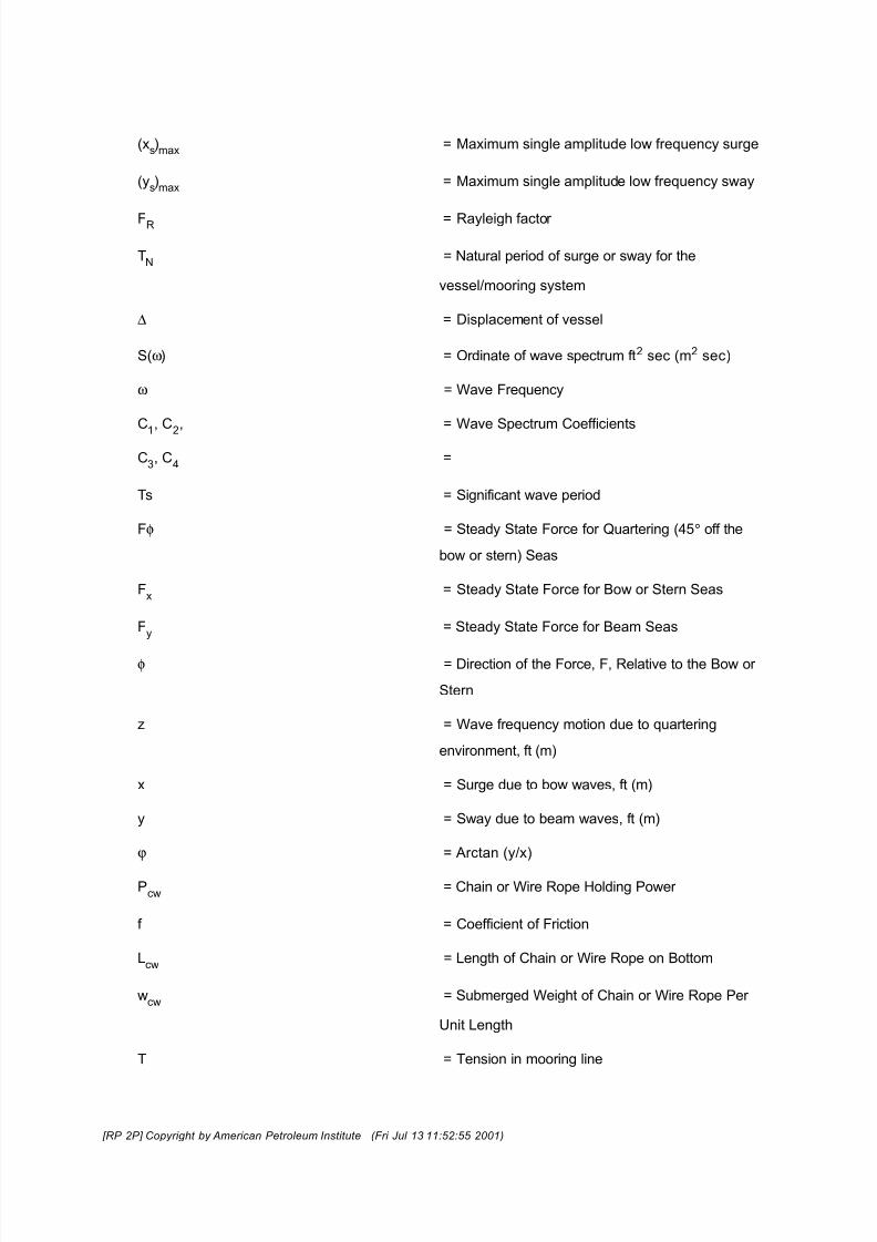
(xs)max
= Maximum single amplitude low frequency surge
(ys)max
= Maximum single amplitude low frequency sway
FR = Rayleigh factor
TN
= Natural period of surge or sway for the
vessel/mooring system
∆ = Displacement of vessel
S(ω) = Ordinate of wave spectrum ft2 sec (m2 sec)
ω = Wave Frequency
C1
, C2
, = Wave Spectrum Coefficients
C3, C
4 =
Ts = Significant wave period
Fφ = Steady State Force for Quartering (45° off the
bow or stern) Seas
Fx
= Steady State Force for Bow or Stern Seas
Fy
= Steady State Force for Beam Seas
φ = Direction of the Force, F, Relative to the Bow or
Stern
z = Wave frequency motion due to quartering
environment, ft (m)
x = Surge due to bow waves, ft (m)
y = Sway due to beam waves, ft (m)
ϕ = Arctan (y/x)
Pcw
= Chain or Wire Rope Holding Power
f = Coefficient of Friction
Lcw
= Length of Chain or Wire Rope on Bottom
wcw
= Submerged Weight of Chain or Wire Rope Per
Unit Length
T = Tension in mooring line
[RP 2P] Copyright by American Petroleum Institute (Fri Jul 13 11:52:55 2001)

8/18/2019 API RP 2P RP
http://slidepdf.com/reader/full/api-rp-2p-rp 8/68
δc
= Elastic stretch of chain
Dc
= Nominal chain diameter
Sc = Chain length
δw
= Elastic stretch of wire rope
Dw
= Nominal diameter of wire rope
Sw
= Wire rope length
β = Coefficient for submerged weight of mooring line
X, Y = Coordinates of Mooring Line Catenary
s = Arc length of Mooring Line Catenary
Ph
= Horizontal Force in Mooring Line Catenary
1.5 Environmental Design Criteria
a. Wind. The design wind speed should be determined based on the statistical wind speed
distribution for the most severe environment in which the mooring system must operate.
Figure 2 illustrates a typical statistical wind speed distribution curve. Curves similar to Figure 2 are
obtained from field data by plotting the cumulative probability versus wind speed, Vw, where the
cumulative probability is the probability of a measured wind speed being equal to or less than Vw. It
should be noted that a cumulative probability of 0.99 for a given Vw does not imply a 100-year
storm condition. It does mean that for the specific population of wind speeds corresponding to the
given site and the anticipated seasons of operation, only one percent of the time the wind speed
will exceed Vw.
The design wind speed for use in the formulas of Section 3.2 should be selected in accordance
with the following criteria:
(1) The average wind speed over a one-minute interval should be used.
(2) The wind speed should pertain to an elevation of 10 meters above still water level.
(3) The cumulative probability for the design wind speed should be 0.999.
(4) The design wind speed should be selected for the most severe season during which operations
are to be conducted at a given site.
Figure 2 illustrates the method of determining the design wind speed from the statistical wind
speed data. Wind speed data used to generate the distribution curve should include available
[RP 2P] Copyright by American Petroleum Institute (Fri Jul 13 11:52:55 2001)

8/18/2019 API RP 2P RP
http://slidepdf.com/reader/full/api-rp-2p-rp 9/68
measured data and storm hindcast data as well as ship's observations.
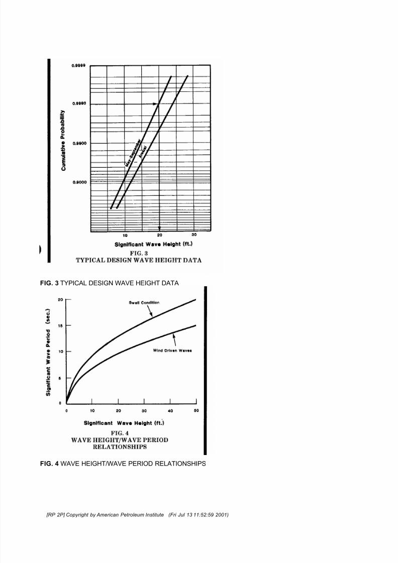
b. Waves. The design wave height should be determined based on the statistical wave height
distribution for the most severe environment in which the mooring system must operate.
Figure 3 illustrates a typical wave height distribution curve. Curves similar to Figure 3 are obtained
from field data by plotting the cumulative probability versus significant wave height, Hs, where the
cumulative probability is the probability that the significant wave height for an observed sea state
will be equal to or less than Hs.
The design sea state is characterized by the design wave height. The design wave height should be
selected in accordance with the following criteria:
(1) The cumulative probability for the design wave height should be 0.999.
(2) The design wave height should be the significant wave height for the design sea state, i.e., the
average of the one-third highest waves.
(3) The design sea state should be selected for the most severe season during which operations
are to be conducted at a given site.
Figure 3 illustrates the method of determining the design wave height from the statistical wave
height data. The wave height data used to generate the distribution curve should include available
measured data and storm hindcast data as well as ship's observations. The wave height versus
wave period relationships for the design sea state should be accurately determined fromoceanographic data for the area of operation. The period can significantly affect surge and sway
amplitudes and mean drift forces. For cases where measured data are not available, Figure 4
provides characteristic wave period versus wave height relationships for wind generated waves and
for predominant swell conditions.
c. Currents. Accurate data for the magnitude, direction, and seasonal variation of surface currents
should be obtained for the area of operations. Based on this data the current speed for design and
operating conditions should be selected.
d. Ice Conditions. Normally the hulls of floating drilling units are not designed to resist to ice loading
in the moored condition.
e. Basis and Special Consideration for the Environmental Design Criteria. The two commonly used
methods to designate the severity of a design environment are:
(1) The cumulative probability method which specifies the percentage of time during the average
year that the environment (seas, wind, or current) will not exceed a given level; and
(2) The return period method which specifies the average recurrence interval between the
occurrence of a given environment.
[RP 2P] Copyright by American Petroleum Institute (Fri Jul 13 11:52:56 2001)

8/18/2019 API RP 2P RP
http://slidepdf.com/reader/full/api-rp-2p-rp 10/68
The cumulative probability method has been adopted by API RP 2P and a 99.9% probability of
nonexceedance is specified as the maximum design environment for mobile drilling units.
As a point of comparison, a storm with a 100-year return period is often specified as the design
environment for fixed platforms, floating production platforms, and floating units operating next to
other offshore installations. However, it would be unduly conservative for mobile drilling units to use
the 100-year environment for the reasons explained below.
There is, in general, no direct correlation between the return period and the probability of
nonexceedance. However, for any given location, reasonable assumptions about the storm duration
and the environmental data base would generally result in a 99.9% environment being considerably
lower than the 100-year environment. The selection of the 99.9% environment is based on the
operational experience of the offshore industry. This, we believe, is a sufficiently conservative
design environment for mooring analysis of mobile drilling units for two reasons. Firstly, the
analysis technique presented in Section 5.2 accounts for collinear environmental forces. However,
when extreme environments are encountered, the winds and waves are generally collinear, but the
currents may not necessarily be collinear with wind and waves.
Secondly, since these units are normally not operating in close proximity to other offshore
structures, the consequences of vessel movement due to overloading the mooring system under an
extreme environment are less severe than those associated with overloading fixed platforms or
floating units which are nearby other structures. Also, since the anchor holding capacity of a
mooring system is normally substantially lower than the breaking strength of the mooring line, a
mooring "failure" normally consists of anchor slippage. Anchor slippage in the most loaded lines
would cause a redistribution of loads among the other mooring lines and, in turn, would reduce the
peak line tensions to substantially lower levels. Vessel displacement caused by this scenario can
normally be tolerated by these units.
Special considerations of exposure risk should be made for drilling vessels operating for an
extended period of time in a single location such as vessels for development drilling. For drilling
programs operating for more than a full year, consideration should be given to the return period
method. In this case, a return period of five times the exposure period should be considered. The
return period environment should be compared to the 99.9% non-exceedance environment, and the
most conservative value used.
1.6 Water Depth.
The water depth at the drilling location should be determined. The slope and direction of the ocean
floor should also be determined to establish the water depth at each anchor.
1.7 Soil Condition.
[RP 2P] Copyright by American Petroleum Institute (Fri Jul 13 11:52:56 2001)

8/18/2019 API RP 2P RP
http://slidepdf.com/reader/full/api-rp-2p-rp 11/68
Bottom soil conditions existing at the drilling location should be determined to provide data for
evaluating anchor performance. In areas with extremely soft soils, piggy back anchors may be
required. In areas with extremely hard bottoms, drilled or driven pile anchors may be necessary.
1.8 Mooring Equipment.
The following information on the mooring equipment should be determined:
a. Mooring Lines. Number, diameter, maximum useable length out from fairlead, submerged weight
per unit length, and catalog breaking strength of mooring lines.
b. Anchors. Number, size and type of anchors. Anchor piles may be evaluated for soil conditions
where the use of conventional anchors is questionable.
c. Pendants. Number, diameter and length of pendants.
d. Deck Machinery. Maximum winch/wildcat pull (at stall) and maximum winch/wildcat brake
capacity.
SECTION 2 MOORING SYSTEM
Typically, mooring systems for mobile drilling units are of the 'spread moored' type wherein fairleads are
located around the periphery of the vessel. Figure 5 depicts a typical spread mooring system for
semisubmersibles and drillships which consists of eight mooring lines with four double drum winches (or
windlasses) located at the four corners of the vessel. Generally, the term winch refers to the machinery
to spool and store wire rope, and a windlass is used to control the mooring chain. The chain is stored
below the windlass in a compartment called chain locker. Some drilling vessels have a winch/windlass
combination system for mooring lines consisting of both wire rope and chain. A mooring line is led to
the seafloor by a fairlead which changes the direction of pull of a mooring line. An anchor is used to fix
the line to the seafloor. A pendant buoy with a pendant line is used for marking and retrieving the
anchor. The length of a mooring line is normally in the range of 3000 to 6000 feet.
A shipshape vessel is subjected to much smaller environmental forces when the weather approaches
the vessel's bow or stern. One operational problem associated with spread moorings for drillships is the
limited ability to rotate the vessel into the predominant weather, thus avoiding high environmental loads
from the beam direction. A turret-moored drillship, as shown in Figure 6, can head into the predominant
environment, minimizing the environmental forces imposed on the vessel. This capability is achieved by
placing the wire rope winches on top of a turret which can rotate with relation to the hull of the vessel.
Powered thrusters are used to rotate the vessel into the weather.
2.1 Mooring Pattern.
Many possible arrangements are available for spacing the mooring lines around a drilling unit.
[RP 2P] Copyright by American Petroleum Institute (Fri Jul 13 11:52:56 2001)

8/18/2019 API RP 2P RP
http://slidepdf.com/reader/full/api-rp-2p-rp 12/68
Normally, orientation of the lines is based on consideration of the type of hull and the surfaces of the
hull exposed to the environment. The beam or side areas of ships and barges are generally larger than
the bow area, so that the mooring lines are arranged to provide greater support on the beam. For
semisubmersibles, approximately the same area is exposed on both the bow and beam, and
symmetric mooring patterns are frequently employed. Final selection of a mooring pattern should be
based on hull type and the prevailing direction of wind, current, and waves. In some areas where
strong winds or currents come from one direction only, strongly asymmetric mooring patterns with
lines concentrated to one side have been used successfully.
Typical mooring patterns are shown in Figure 7. The most commonly used patterns are the 30-60°
eight line (Figure 7a) and the symmetric eight line Figure 7b). In some areas where strong wind or
current comes from a predictable direction, skewed mooring patterns as illustrated in Figure 7g have
been successfully used. Asymmetric mooring patterns are sometimes used when pipelines or
shipping fairways are in close proximity of the drill site (Figure 7h).
2.2 Type of Mooring.
Mooring systems of floating drilling vessels can be divided into three categories: an all wire rope
system, an all chain system, and a chain/wire rope combination system. Advantages and limitations
of each system are discussed below.
a. All Wire Rope System. Wire rope is more lightweight than chain. Therefore, in general, wire rope
provides more restoring force in deep water than chain and requires lower pretensions. However, to
prevent anchor uplift, much longer line length is required for an all wire rope system. Also, wear due
to abrasion between wire rope and a hard seafloor can sometimes become a problem. Moreover,
wire rope needs careful maintenance. Corrosion due to lack of lubrication or mechanical damage to
the wire rope could cause mooring failure.
b. All Chain System. Chain has shown durability in offshore operations. It has better resistance to
bottom abrasion and contributes significantly to anchor holding capacity. However, because of its
heavy weight, it is undesirable for deepwater operations. During anchor deployment, chain requires
windlasses with large shaft horsepower and brake capacities. In addition, anchor handling boats
must have larger bollard pull capacities to deploy the anchors.
c. Chain/Wire Rope Combination System. In this system, the chain is outboard between the anchor
and the wire rope. By proper selection of the length of wire rope, a combination system offers the
advantages of low pretension requirement, high restoring force, added anchor holding capacity, and
good resistance to bottom abrasion. These advantages make it the best system for deepwater
operations. Semisubmersibles with chain/wire rope combination mooring which are capable of
drilling in 5,000 feet of water in hostile environments have been built. Anchor deployment and
retrieval are sometimes more time consuming with a combination system, and workboats with
[RP 2P] Copyright by American Petroleum Institute (Fri Jul 13 11:52:56 2001)

8/18/2019 API RP 2P RP
http://slidepdf.com/reader/full/api-rp-2p-rp 13/68
chain lockers are often required to store the chain. However, new combination winch/windlass
systems that eliminate the need for workboats with chain lockers are available today, and the time
for making the wire rope/chain connections can be markedly reduced or eliminated.
SECTION 3 ENVIRONMENTAL FORCES AND VESSEL MOTIONS
3.1 Basic Considerations.
The recommended mooring analysis procedure outlined in Section 5 requires the evaluation of forces
on the drilling unit due to wind, waves, and currents and the evaluation of oscillatory displacements
due to waves. Wind, waves, and current each produces a steady state force. These forces are
evaluated individually and summed to get the total steady state environmental force. This steady state
force produces a steady state displacement which is a function of the stiffness of the mooring
system. The total displacement is equal to the sum of the oscillatory wave displacement and the
steady state displacement. The loads and stresses in the mooring system are then evaluated based
on the total displacement and the stiffness of the mooring system.
Oscillatory wave displacements are computed for free floating hulls neglecting the restraint provided
by the mooring system. For normal hull forms and mooring system configurations the restraint
provided by the mooring system does not appreciably affect the wave frequency component of the
horizontal displacement due to waves. However, it significantly affects the low frequency component.
3.2Wind.
The force due to wind may be determined by using wind tunnel model test data or equations given in
this section. The wind speed used is defined in Section 1.5a.
a. Model Tests. Model test data may be used to predict wind loads for mooring system design
provided that a representative model of the unit is tested, that the unit is tested in a credible facility,
and that the condition of the model in the tests, i.e., draft, deck cargo arrangement, etc., closely
matches the expected conditions that the unit will see in service. Care should also be taken to
assure that the character of the flow in the model test is the same as the character of flow for the
full scale unit.
b. Wind Force Calculation. The force due to wind acting on a moored drilling unit should be
determined using Equation 3.1.
(3.1) Fw = C
wΣ(C
sC
h A)V2
w
Where
Fw
= wind force, lbs (N)
Cw = 0.0034 lb/(ft2 · kt2)(0.615 Nsec2/m4)
[RP 2P] Copyright by American Petroleum Institute (Fri Jul 13 11:52:56 2001)
8/18/2019 API RP 2P RP
http://slidepdf.com/reader/full/api-rp-2p-rp 14/68
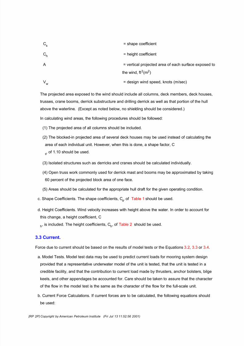
Cs
= shape coefficient
Ch
= height coefficient
A = vertical projected area of each surface exposed to
the wind, ft2(m2)
Vw
= design wind speed, knots (m/sec)
The projected area exposed to the wind should include all columns, deck members, deck houses,
trusses, crane booms, derrick substructure and drilling derrick as well as that portion of the hull
above the waterline. (Except as noted below, no shielding should be considered.)
In calculating wind areas, the following procedures should be followed:
(1) The projected area of all columns should be included.
(2) The blocked-in projected area of several deck houses may be used instead of calculating the
area of each individual unit. However, when this is done, a shape factor, C
s, of 1.10 should be used.
(3) Isolated structures such as derricks and cranes should be calculated individually.
(4) Open truss work commonly used for derrick mast and booms may be approximated by taking
60 percent of the projected block area of one face.
(5) Areas should be calculated for the appropriate hull draft for the given operating condition.
c. Shape Coefficients. The shape coefficients, Cs, of Table 1 should be used.
d. Height Coefficients. Wind velocity increases with height above the water. In order to account for
this change, a height coefficient, C
h, is included. The height coefficients, C
h, of Table 2 should be used.
3.3 Current.
Force due to current should be based on the results of model tests or the Equations 3.2, 3.3 or 3.4.
a. Model Tests. Model test data may be used to predict current loads for mooring system design
provided that a representative underwater model of the unit is tested, that the unit is tested in a
credible facility, and that the contribution to current load made by thrusters, anchor bolsters, bilge
keels, and other appendages be accounted for. Care should be taken to assure that the character
of the flow in the model test is the same as the character of the flow for the full-scale unit.
b. Current Force Calculations. If current forces are to be calculated, the following equations should
be used:
[RP 2P] Copyright by American Petroleum Institute (Fri Jul 13 11:52:56 2001)

8/18/2019 API RP 2P RP
http://slidepdf.com/reader/full/api-rp-2p-rp 15/68
(1) Force due to bow or stern current on ship-shaped hulls.
(3.2) Fcx
= Ccx
SV2c
Where
Fcx
= current force on the bow, lb (N)
Ccx
= current force coefficient on the bow
= 0.016 lb/(ft2 • kt2)(2.89 N sec2/m4)
S = wetted surface area of the hull including
appendages, ft2 (m2)
Vc = design current speed, kts (m/sec)
(2) Force due to beam current on ship-shaped hulls.
(3.3) Fcy
= Ccy
S Vc2
Where
Fcy
= current force on the beam, lb (N)
Ccy
= current force coefficient on the beam
= 0.40 lb/(ft2
· kt2
)(72.37 N sec2
/m4
)
(3) Force due to current on semisubmersible hulls.
(3.4) Fcs
= Css
(Cd A
c + C
d A
f )V2
c
Where
Fcs
= current force, lb (N)
Css
= current force coefficient for semisubmersible hulls
= 2.85 lb/(ft2 · kt2)(515.62 N sec2/m4)
Cd
= drag coefficient (dimensionless)
= 0.50 for circular members. See Figure 8 for
members having flat surfaces.
Ac
= summation of total projected areas of all
cylindrical members below the waterline, ft2 (m2)
Af
= summation of projected areas of all members
[RP 2P] Copyright by American Petroleum Institute (Fri Jul 13 11:52:56 2001)

8/18/2019 API RP 2P RP
http://slidepdf.com/reader/full/api-rp-2p-rp 16/68
having flat surfaces below the waterline, ft2(m2)
3.4 Steady Drift Force.
Three wave related phenomena affect mooring system design. They are: 1) steady state mean drift
force, 2) surge, sway, and yaw response at or near the predominant period of the waves, and 3)
oscillatory drift forces at or near the natural period of the spring/mass system of the moored vessel.
The steady state mean drift forces are typically much smaller than the wave forces that excite surge
and sway response. However, drift forces may still contribute significantly to the total mean
environmental force acting on the vessel. Therefore, wave drift forces should be accounted for in the
mooring system design.
Mean wave drift forces may be predicted using model tests or using advanced hydrodynamic
computer analysis. In the absence of available wave drift force predictions, the following procedure for
estimating mean wave drift force may be used. This procedure uses design curves for typical drillships
and semisubmersibles to facilitate calculation. These design curves were generated by an advanced
vessel motions computer program which has been verified and calibrated by extensive model test
data.
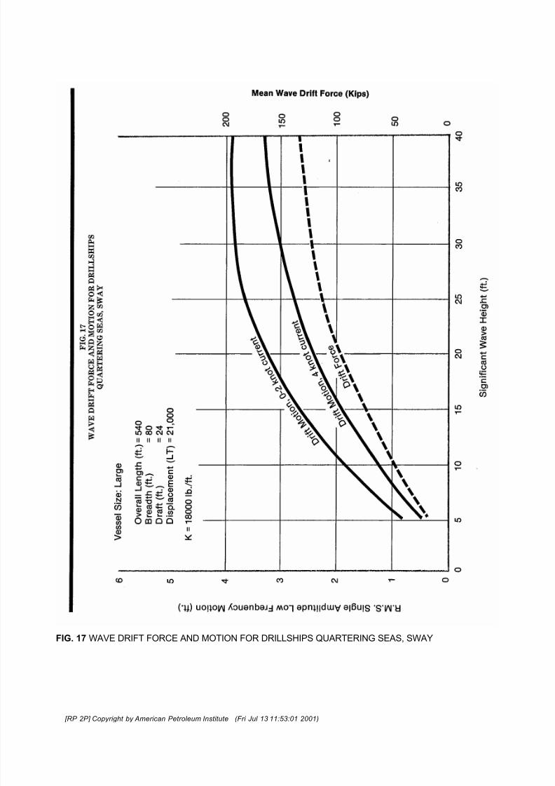
a. Mean Drift Force For Ship-Shaped Hulls. The mean wave drift force for ship-shaped hulls in bow,
quartering and beam seas can be estimated by
Figures 9 through 20, according to the size of the vessel and the direction of the waves relative tothe hull. Drift forces for stern and stern quartering seas are nearly equal to bow and bow quartering
values, respectively.
The curves in these Figures are for drillships of 400 ft to 540 ft length. For drillships which are
outside this length range, the mean drift force can be estimated by extrapolation or the procedure
described below.
Let:
(3.5a - 3.5b)
where (Fmdx
)REF
and (Fmdy
)REF
are bow mean wave drift force (Figures 9-14) and beam mean wave
drift force (Figures 15- 20), respectively, for the reference ship which most closely fits the ship at
hand, taken at a significant wave height of
[RP 2P] Copyright by American Petroleum Institute (Fri Jul 13 11:52:56 2001)
8/18/2019 API RP 2P RP
http://slidepdf.com/reader/full/api-rp-2p-rp 17/68
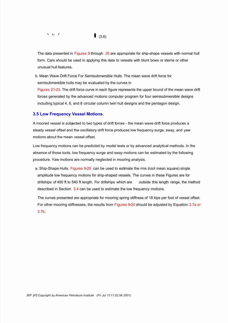
(3.6)
The data presented in Figures 9 through 20 are appropriate for ship-shape vessels with normal hull
form. Care should be used in applying this data to vessels with blunt bows or sterns or other
unusual hull features.
b. Mean Wave Drift Force For Semisubmersible Hulls. The mean wave drift force for
semisubmersible hulls may be evaluated by the curves in
Figures 21-23. The drift force curve in each figure represents the upper bound of the mean wave drift
forces generated by the advanced motions computer program for four semisubmersible designs
including typical 4, 6, and 8 circular column twin hull designs and the pentagon design.
3.5 Low Frequency Vessel Motions.
A moored vessel is subjected to two types of drift forces - the mean wave drift force produces a
steady vessel offset and the oscillatory drift force produces low frequency surge, sway, and yaw
motions about the mean vessel offset.
Low frequency motions can be predicted by model tests or by advanced analytical methods. In the
absence of those tools, low frequency surge and sway motions can be estimated by the following
procedure. Yaw motions are normally neglected in mooring analysis.
a. Ship-Shape Hulls. Figures 9-20 can be used to estimate the rms (root mean square) singleamplitude low frequency motions for ship-shaped vessels. The curves in these Figures are for
drillships of 400 ft to 540 ft length. For drillships which are outside this length range, the method
described in Section 3.4 can be used to estimate the low frequency motions.
The curves presented are appropriate for mooring spring stiffness of 18 kips per foot of vessel offset.
For other mooring stiffnesses, the results from Figures 9-20 should be adjusted by Equation 3.7a or
3.7b,
[RP 2P] Copyright by American Petroleum Institute (Fri Jul 13 11:52:56 2001)

8/18/2019 API RP 2P RP
http://slidepdf.com/reader/full/api-rp-2p-rp 18/68

8/18/2019 API RP 2P RP
http://slidepdf.com/reader/full/api-rp-2p-rp 19/68
represents the upper bound of the low frequency vessel motions generated by the advanced
motions computer program for four semisubmersible designs including typical 4, 6, and 8 circular
column twin hull designs and the pentagon design.
3.6 Wave Frequency Vessel Motions.
The motions of the vessel at the frequency of the waves is an important contribution to the total
mooring system loads, particularly in shallow water. These wave frequency motions can be obtained
from random wave model test data, or computer analysis using either time or frequency domain
techniques. In the absence of these tools, the following approach can be used to estimate the wave
frequency motions.
a. Spectral Analysis Method. The evaluation of wave displacement by the method of spectral
analysis involves first determining the response spectrum as a function of frequency over the full
range of wave frequencies. The response spectrum is then integrated and the square root is taken
to determine the rms response. Finally the significant and maximum responses can be obtained
by using appropriate Rayleigh factors. The specific recommended procedure is outlined in detail in
the following sections, and an example calculation is provided in
Section 6. The procedure has been simplified in the following respects.
(1) The wave spectrum is considered to be unidirectional, i.e., no wave spreading function is
considered.
(2) No coupling of motions is considered.
The spectral analysis method has been shown to agree with measured wave displacements with
errors on the order of 10% to 20%. This amount of error is considered "state of the art" and the
safety factors of Section 4 have been selected to account for such errors and to yield designs
which are consistent with proven field experience.
b. The Design Wave Spectrum. Appropriate design wave spectra for a specific geographical area
may be available from meteorological consultants; however, it is more likely that sea state data will
be available in the form of significant wave height, and period versus cumulative frequency of
occurrence or in the form of wind speed versus cumulative frequency of occurrence as illustrated in
Figures 2 and 3. In this case the significant wave height, significant wave period and design wind
speed corresponding to the operating condition and the design condition should be determined as
outlined in Section 1.5. Then for each condition, the corresponding wave spectrum may be
evaluated using either Equation 3.11 or Equation 3.12.
[RP 2P] Copyright by American Petroleum Institute (Fri Jul 13 11:52:56 2001)

8/18/2019 API RP 2P RP
http://slidepdf.com/reader/full/api-rp-2p-rp 20/68
(3.11 - 3.12)
Equations 3.11 and 3.12 will not normally yield exactly the same spectrum; one or the other should
be selected depending on whether wave height data or wind speed data are considered to be more
reliable for the geographical area under consideration. If the value of Ts is not available from
oceanographic data, the appropriate value may be estimated using Figure 4. The design wave
height, Hs, is the significant wave height in the statistical sense, i.e., the average of the 1/3 highest
waves. The value of Ts is the corresponding wave period. The design wind speed is the same as
defined in Section 1.5a.
The wave spectrum defined by Equations 3.11 and 3.12 is known as the ISSC spectrum. Other
wave spectra such as the Pierson-Moskowitz spectrum, Bretschneider spectrum, and the Jonswap
spectrum can be used if they are more appropriate for the drilling location under consideration.
c. Response Amplitude Operators. Motion response operators for surge in head seas and sway in
beam seas should be available from carefully conducted model tests over a full range of wave
frequencies. Analytical motion response operators obtained by integrating wave pressure over the
wetted surface of the drilling unit and solving the basic equations of motion, may also be used.
Care should be taken to assure that curves are for single amplitude response per unit wave
amplitude. In the absence of model test data or analytical curves, the response operators of
Figures 24, 25 and 26 may be used. Response operators are given for three classes of
semisubmersible drilling units and two classes of ship-shape drilling units. Response operators for
intermediate class units may be interpolated. Characteristics of the various classes of drilling units
are tabulated in Table 3.
[RP 2P] Copyright by American Petroleum Institute (Fri Jul 13 11:52:56 2001)

8/18/2019 API RP 2P RP
http://slidepdf.com/reader/full/api-rp-2p-rp 21/68

8/18/2019 API RP 2P RP
http://slidepdf.com/reader/full/api-rp-2p-rp 22/68
SECTION 4 MOORING DESIGN CRITERIA
4.1Offset
a. Definition of Mean Offset. The mean offset is defined as the vessel displacement due to the
combination of wind, current, and mean wave drift forces.
b. Definition of Maximum Offset. The maximum offset is the mean offset plus appropriately combined
wave frequency and low frequency vessel motions. Maximum offset can be determined by the
following procedure.
Let:
(WF)max
= Maximum wave frequency motion
(WF)1/3
= Significant wave frequency motion
(LF)max
= Maximum low frequency motion
(LF)1/3
= Significant low frequency motion
(1) If (LF)max
> (WF)max
, then Maximum offset = Mean offset + (LF)max
+ (WF)1/3
(2) If (WF)max
> (LF)max
, then Maximum offset = Mean offset + (WF)max
+ (LF)1/3
A parametric study has been performed to assess the risk level associated with this method of
combining wave and low frequency motions. The chance of exceeding the combined motions
defined above was estimated using a probabilistic approach for different hull forms, water depths,
environments, and types of mooring. The results of the study indicate that the combined low and
wave frequency motions defined in this manner would be exceeded approximately once in three
hours. This appears a proper risk level for the operations addressed by this Recommended
Practice.
c. Offset Limits. The offsets of the drilling unit from the wellbore must be controlled to prevent
damage to the drilling riser and the BOP stack.
(1) Maximum Operating Condition. The mean offset should be controlled under the operating
condition because of its direct relevance to the mean ball joint angle. The allowable mean offset
should be determined by a drilling riser analysis. Allowable mean offsets depend on many
factors such as water depth, environment, and riser system. They normally fall in a range of
2.5% to 6% of water depth. Generally the lower bound applies to deepwater (1500-2000 ft)
operations, and the upper bound applies to shallow water (200-300 ft) operations.
(2) Maximum Connected Condition. The maximum offset should be controlled under the maximum
connected condition to prevent damage to the mechanical stop in the ball joint below the drilling
[RP 2P] Copyright by American Petroleum Institute (Fri Jul 13 11:52:57 2001)
8/18/2019 API RP 2P RP
http://slidepdf.com/reader/full/api-rp-2p-rp 23/68
riser. The allowable maximum offset should be determined by a drilling riser analysis. Allowable
maximum offsets depend on many factors such as water depth, environment, and riser system.
They normally fall in a range of 8% to 12% of water depth. Generally the lower bound applies to
deep water (1500-2000 ft) operations, and the upper bound applies to shallow water (200-300 ft)
operations.
(3) Maximum Design Condition. For the maximum design condition, if the riser is disconnected
from the well, there is no restriction on vessel offset. Design criteria for this condition consists
only of restrictions on loads in the mooring lines.
4.2 Maximum Mooring Line Tension.
The maximum mooring line tension is calculated at the maximum vessel offset. The tension in the
most loaded line at the design condition should not exceed 50% of the ultimate strength of the line.
The ultimate strength of the line may be taken as the catalog break strength (CBS) of the wire rope
(provided it is new or in like new condition). Worn rope should be limited to lesser design loads. The
ultimate strength of chain may be taken as the break test load (BTL) provided the chain is new or in
like-new condition. Used or worn chain should be limited to lesser design loads. The tension in the
most loaded line at the maximum operating condition should not exceed 33% of the ultimate strength
of the line. Mooring line adjustments to alleviate tensions can be considered in the analysis.
4.3 Line Length.
The mooring line (outboard line) length should be sufficient to allow the lines to come in tangent to the
ocean bottom at the anchor when the system reaches the maximum anticipated offset.
4.4 Drag Anchor Holding Power.
Floating drilling units are commonly moored with drag anchors. In hard-to-anchor bottom soil
conditions, anchor piles and explosive embedment anchors are sometimes used. The following
discussion will address the holding power of drag anchors only.
The holding power of a drag anchor in a particular soil condition represents the maximum sustained
horizontal load the anchor will resist in that soil before dragging. The length of mooring chain or wire
connected to the anchor that remains on the bottom soil will also contribute to the holding power of
that mooring line and will reduce the horizontal load imposed on the anchor.
a. Anchor Holding Power. Anchor holding power is a function of several factors, including the
following:
1) Anchor type - Fluke area, fluke angle, fluke smoothness, anchor weight, tripping palms,
stabilizer bars, etc.
[RP 2P] Copyright by American Petroleum Institute (Fri Jul 13 11:52:57 2001)
8/18/2019 API RP 2P RP
http://slidepdf.com/reader/full/api-rp-2p-rp 24/68
2) Bottom soil condition - Soft mud, sand, gravel, clay, rock, coral, etc.
3) Anchor behavior during deployment - Opening of the flukes, penetration of the flukes, depth of
burial of the anchor, stability of the anchor during dragging, soil behavior over the flukes, etc.
Due to the wide variation of these factors, the prediction of an anchor's holding power is difficult.
Exact holding power can only be determined after the anchor is deployed and test loaded.
Anchor performance data for the specific anchor type and soil condition should be obtained if
possible. In the absence of credible anchor performance data, Figures 27 and 28 may be used to
estimate the holding power of anchors commonly used to moor floating drilling units.
Figures 27 and 28 are from "Handbook for Marine Geotechnical Engineering," Naval Civil
Engineering Laboratory, 1985. There are other sources of data on anchor holding capacity.
Sometimes there are significant differences among the prediction curves from different sources
because of differences in test conditions (size of anchor, type of soil, and test hardware) and test
data interpretation. Furthermore, some of the anchors such as the Bruce anchor and the Stevpris
anchor have been modified recently. The performances of the modified anchors can be substantially
different from those predicted by these figures.
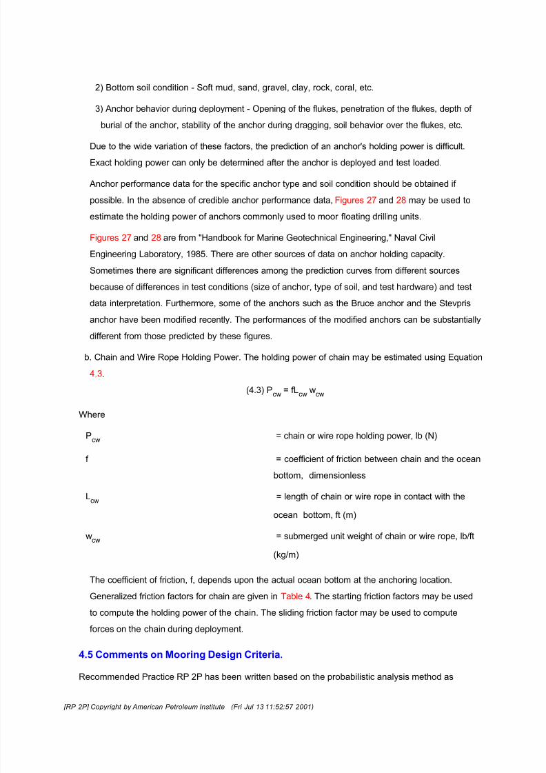
b. Chain and Wire Rope Holding Power. The holding power of chain may be estimated using Equation
4.3.
(4.3) Pcw
= fLcw
wcw
Where
Pcw
= chain or wire rope holding power, lb (N)
f = coefficient of friction between chain and the ocean
bottom, dimensionless
Lcw
= length of chain or wire rope in contact with the
ocean bottom, ft (m)
wcw
= submerged unit weight of chain or wire rope, lb/ft
(kg/m)
The coefficient of friction, f, depends upon the actual ocean bottom at the anchoring location.
Generalized friction factors for chain are given in Table 4. The starting friction factors may be used
to compute the holding power of the chain. The sliding friction factor may be used to compute
forces on the chain during deployment.
4.5 Comments on Mooring Design Criteria.
Recommended Practice RP 2P has been written based on the probabilistic analysis method as
[RP 2P] Copyright by American Petroleum Institute (Fri Jul 13 11:52:57 2001)

8/18/2019 API RP 2P RP
http://slidepdf.com/reader/full/api-rp-2p-rp 25/68
opposed to the more traditional deterministic analysis method. This choice was made because the
design environments and motions of a floating hull in a random sea can be more accurately described
in probabilistic terms.
The three primary factors in any design for offshore installations are the environmental criteria, the
load analysis procedures, and the allowable stress and deflection criteria. For example, API RP 2P
specifies that the appropriately combined low and wave frequency vessel motions be used with a
safety factor of 2.0 relative to the line breaking strength, for checking line tensions in conjunction with
the 99.9% environment. The selection of this combination of design environment, statistical level of
vessel motions, and safety factor is empirical and based on operational experience and judgment. It is
important to note that the level of vessel motions (maximum, significant, etc.) and the safety factor
cannot be selected independently of the maximum design environment since taken together they
define the total risk level.
Since the RP 2P analysis method is somewhat of a break with tradition for the offshore industry, there
may be a tendency to adopt certain portions of the method and reject the others; for instance, the
mooring analysis procedures and tension criteria might be applied with the 100-year storm design
environment. This would result in a gross, unwarranted increase in system reliability over what has
proven safe and economical in many rig-years of experience. This Recommended Practice does not
address an analysis method for evaluating the mooring system's capability in extreme events such as
100-year storm conditions in severe environmental areas, and therefore, it is recommended that this
analysis method not be used for such analyses.
It should be emphasized that the selective use of the mooring analysis procedures out of context can
lead to misleading results. In RP 2P, wind loads, current loads, mean wave loads, and vessel surge
motions are specifically accounted for; however, contributions due to bending over fairleaders, line
dynamics, vessel heave, pitch, and roll motions, etc., are not computed specifically. These
contributions are usually not the major factors influencing mooring line loads in drilling applications,
and are therefore lumped together and accounted for by a safety factor on the maximum allowable
mooring line load. If a more comprehensive mooring analysis is made, for example, dynamic mooring
analysis, corresponding change in allowable load can be justified.
SECTION 5 MOORING ANALYSIS PROCEDURE
5.1 Basic Considerations.
The general procedure outlined below is recommended for the analysis of mooring systems for floating
drilling units. Systems designed in accordance with this procedure and satisfying the design criteria
as defined in Section 4 should be adequate for the selected environment. Use of this procedure is
illustrated in the example of Section 6.
[RP 2P] Copyright by American Petroleum Institute (Fri Jul 13 11:52:57 2001)
8/18/2019 API RP 2P RP
http://slidepdf.com/reader/full/api-rp-2p-rp 26/68

8/18/2019 API RP 2P RP
http://slidepdf.com/reader/full/api-rp-2p-rp 27/68
(5.1) T/δc = 1.2 × 10⁷D
c2/S
c
where:
T = mooring line tension (lbs)
δc
= elastic stretch of chain (feet)
Dc
= nominal chain diameter (in)
Sc
= chain length (feet)
For wire rope:
(5.2) T/δw = 7.7 × 10⁶D
w2/S
w
where:
δw
= elastic stretch of wire rope (feet)
Dw
= nominal diameter of wire rope (in.)
Sw
= wire rope length (feet)
The stretch coefficient for wire rope in Equation (5.2) is appropriate for six strand wire ropes
commonly used in mooring applications. For other types of wire rope such as spiral strand the
stretch coefficient may differ.
The recommended values for the submerged weight of wire rope or chain per unit length can be
calculated by Equation 5.3.
(5.3) Submerged weight = weight in air × β
β = 0.87 (chain)
β = 0.83 (wire rope)
b. Enter the force versus offset curve for the total mooring system at the restoring force required to
withstand the steady state environmental force.
c. Determine the vessel's mean offset and mean line tension corresponding to the above steady
state force.
d. Add the maximum single amplitude motion to the mean offset to determine the maximum vessel
offset and maximum line tension. The maximum single amplitude motion is defined as the properly
combined wave frequency and low frequency motions. (Section
4.1)
e. Determine the maximum suspended line length. To avoid anchor uplift, the maximum suspended
[RP 2P] Copyright by American Petroleum Institute (Fri Jul 13 11:52:57 2001)

8/18/2019 API RP 2P RP
http://slidepdf.com/reader/full/api-rp-2p-rp 28/68
line length should be less than the outboard mooring line length.
f. Determine the maximum anchor load.
(5.4) Maximum anchor load = maximum line tension − (unit submerged weight of mooring line) ×
(water depth) − friction between mooring line and seafloor.
Compare the calculated anchor loads with those predicted by Fig. 28 and 29 or by other available
data for anchor holding power. Because of the uncertainties in anchor performance prediction, a
factor of safety may be considered.
g. Check the calculated line tensions and offsets against the mooring design criteria. If the mooring
criteria are not met, change the mooring system and perform the analysis again. Possible mooring
system changes include changes in initial tension, mooring line length, and mooring pattern.
SECTION 6 EXAMPLE ANALYSIS
6.1 Example Definition.
The following example demonstrates the use of this Recommended Practice.
a. Drilling Unit Description. The drilling unit is a 10,000-ton drillship, 360 ft. × 70 ft. × 24 ft., and
operates at a draft of 17.0 ft. Beam and bow profiles are shown in Figure 31. The total wetted area
of the submerged hull, S, corrected for all appendages, is 36,600 ft.2
b. Mooring System Description
(1) Mooring Lines: 8 6,000 ft. 2.75 in. IWRC wire rope. Catalogue breaking strength (CBS) =
695 kips; Weight = 13.4 lb/ft. in air, and 11.1 lb/ft. in water; AE = 58,231 kips.
(2) Anchor: 8 - 30 kip LWT type.
(3) Mooring Pattern: 30°-60°
(4) Initial Line Tension: 75 kips.
c. Environmental Condition. Table 5 presents the maximum operating and the maximum design
environmental conditions. The maximum connected condition is assumed to be the same as the
maximum design condition.
6.2 Mooring Analysis for the Maximum Design Condition
a. Wind Force
(1) Beam Wind Force (Fig. 31)
[RP 2P] Copyright by American Petroleum Institute (Fri Jul 13 11:52:57 2001)

8/18/2019 API RP 2P RP
http://slidepdf.com/reader/full/api-rp-2p-rp 29/68
(2) Bow Wind Force. By similar procedure, we obtain:
Fwx = .0034 (9380)(542)
= 93,000 lb.
(3) Quartering Wind Force (Equation 3.13)
φ = 45°
EQUATION
b. Current Force
(1) Bow Current Force (Eq. 3.2)
Fcx
= Ccx
SVc2
= 0.016(36,600)22
= 2340 lbs.
(2) Beam Current Force (Eq. 3.3)
Fcy
= Ccy
SVc2
= 0.4 (36,600)22
= 58,560 lbs.
(3) Quartering Current Force. Using Equation 3.13, with φ = 45°, we obtain
[RP 2P] Copyright by American Petroleum Institute (Fri Jul 13 11:52:57 2001)

8/18/2019 API RP 2P RP
http://slidepdf.com/reader/full/api-rp-2p-rp 30/68
Fcz
= 2/3(Fcx
+ Fcy
)
= 40,600 lbs.
c. Mean Wave Drift Force
(1) Bow Wave Drift Force. To simplify calculation, this can be classified as a small size vessel.
Using Fig. 9, for a significant wave height of 20 ft., we obtain:
Fmdx
= 10.5 kips
Note that the ship length at hand is 360 ft. while the length of the reference ship in Fig. 9 is 400
ft. If more accurate results are desired, adjustments for ship length should be made using Eqs.
3.5 and 3.6.
(2) Beam Wave Drift Force. By similar procedure, we obtain:
Fmdy
= 70.5 kips (Fig. 18)
(3) Quartering Wave Drift Force
d. Wave Frequency Motion (Single Amplitude)
(1) Design Wave Spectrum
(Equation 3.11)
(6.1)
(2) Surge Response Evaluation (Bow Sea). The surge response can be evaluated by the following
steps:
Step 1 - Select a frequency range and an increment. For this example problem, a frequency
range of 0.12 -1.44 rad/sec and an increment
∆w of 0.12 rad/sec are selected.
Step 2 - Determine the surge response amplitude operator (RAO) at each frequency by using
the Class I curve in
[RP 2P] Copyright by American Petroleum Institute (Fri Jul 13 11:52:57 2001)

8/18/2019 API RP 2P RP
http://slidepdf.com/reader/full/api-rp-2p-rp 31/68
Figure 25.
Step 3 - Determine S(ω) at each frequency using Equation 6.1.
Step 4 - Determine the response spectrum which is equal to (RAO)
2
·S(ω).
Step 5 - Find the area under the response spectrum and calculate the rms single amplitude
response.
Step 6 - Apply proper Rayleigh factors to obtain the significant and maximum responses.
This procedure is illustrated by the following table.
(3) Sway Response Evaluation (Beam Sea). By similar procedure, we obtain the following sway
responses:
yrms
= 4.59 ft.
y1/3
= 9.19 ft.
ymax
= 17.09 ft.
(4) Response Evaluation for Quartering Sea
[RP 2P] Copyright by American Petroleum Institute (Fri Jul 13 11:52:58 2001)

8/18/2019 API RP 2P RP
http://slidepdf.com/reader/full/api-rp-2p-rp 32/68
e. Low Frequency Motion (Single Amplitude)
(1) Mean (static) Offset and Mooring Stiffness. Tables 6 and 7 give the mean offset and the
mooring system stiffness at the mean offset.
(2) Surge Response Evaluation (Bow Sea). From Figure 9 the rms low frequency motion
corresponding to the wave height of 20 ft. is
(xs)REF = 1.3 ft.
xs
= 1.3(18/k)½ = 2.08 ft. (Equation 3.7a)
(xs)1/3
= 2xs (Equation 3.8a)
= 4.16 ft.
TN
= 2√∆/K= 2√10,000/7(Equation 3.10)
= 75.6 seconds
FR
=
(Equation 3.9c)
(xs)max
= (xs)1/3
· FR
= 6.55 ft.
(3) Sway Response Evaluation (Beam Sea). By similar procedure, we obtain:
(ys)1/3
= 11.08 ft.
(ys)max
= 17.62 ft.
(4) Quartering Response Evaluation. Using Figures 12 and 15, the rms surge and sway
corresponding to a significant wave height of 20 ft. are 1.3 ft. and 2.2 ft., respectively.
[RP 2P] Copyright by American Petroleum Institute (Fri Jul 13 11:52:58 2001)

8/18/2019 API RP 2P RP
http://slidepdf.com/reader/full/api-rp-2p-rp 33/68
f. Summary of Environmental Forces and Vessel Motions. Table 6 summarizes the environmental
forces and vessel motions.
g. Calculation of Vessel Offset, Maximum Line Tension, Suspended Line Length, and Maximum
Anchor Load.
(1) Bow Environment. The total steady state force is 105.8 kips (Table 6). Using Fig. 32, the mean
offset corresponding to this force is 16.5 ft. Adding the maximum combined wave and low
frequency motion of 11.4 ft. (Table 6), we obtain the maximum vessel offset of 27.9 ft. The
maximum line tension corresponding to this offset is 128.4 kips (18.5% of CBS), and the
maximum suspended line length is 3518 ft. (Fig. 32). The holding capacity of wire rope is:
Pwc = fLwc
Wwc
(Equation 4.3)
= 0.6(6000-3518)11.1
= 16,500 lbs.
By Equation 5.4,
Maximum anchor
load = 128,400 − 11.1 × 550− 16,500 = 105,800 lbs.
(2) Beam Environment and Quartering Environment. By similar procedure, we obtain the resultsfor beam and quartering environments as presented in Table 7.
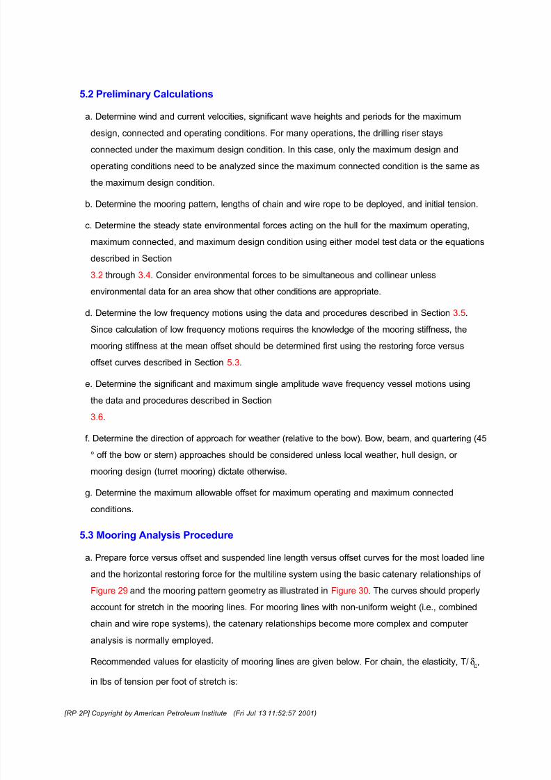
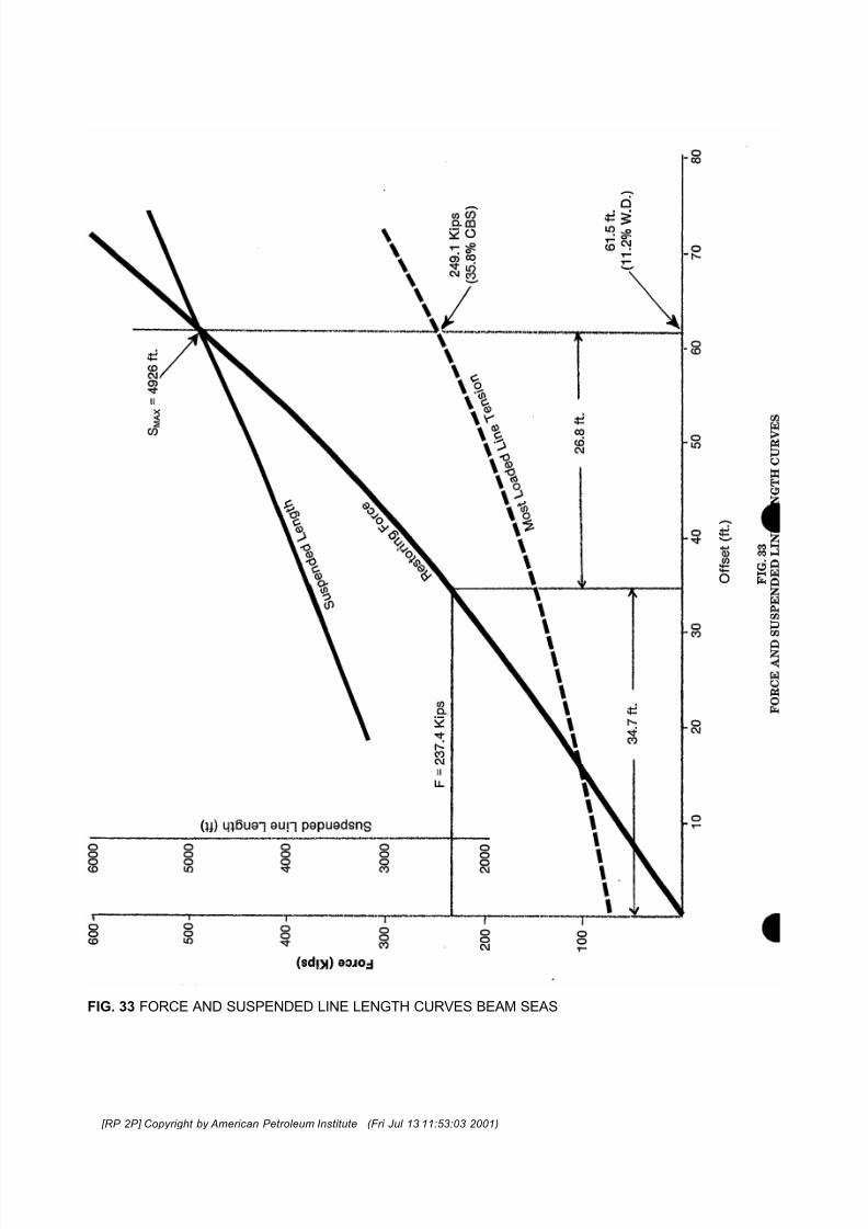
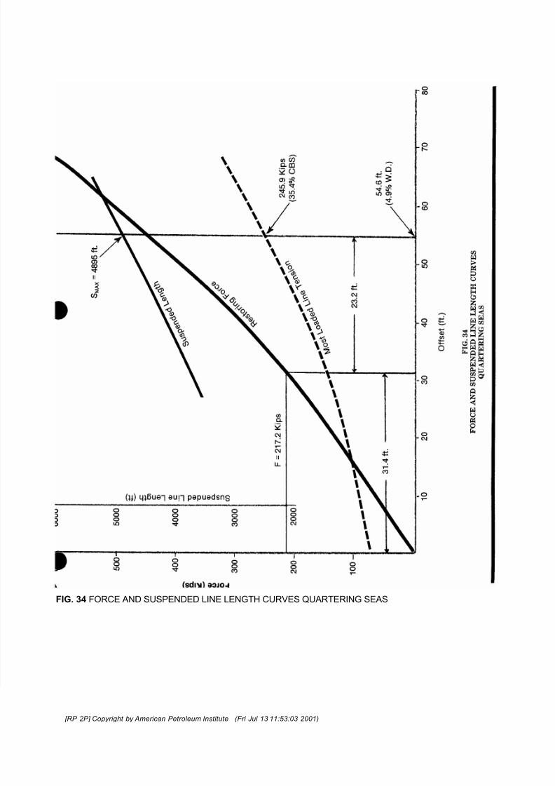
6.3 Mooring Analysis for the Maximum Operating Condition.
By similar procedure and using Figures 33 and 34, we obtain the results for the maximum operating
condition as presented in Tables 8 and 9. Table 8 summarizes the environmental forces and vessel
motions; Table 9 summarizes the vessel offset, maximum line tension, suspended line length, and
maximum anchor load.
6.4 Summary and Discussion of Mooring Analysis Results.
[RP 2P] Copyright by American Petroleum Institute (Fri Jul 13 11:52:58 2001)

8/18/2019 API RP 2P RP
http://slidepdf.com/reader/full/api-rp-2p-rp 34/68
Table 10 summarizes the mooring analysis results. The most critical environment is the beam
environment. The maximum line tension under the maximum operating condition is 20.6% of CBS,
which is less than the recommended tension limit of 33% of CBS. The maximum line tension under
the maximum design condition is 35.5% of CBS, which is less than the recommended tension limit of
50% of CBS.
The mean offset of 3.0% of water depth under the maximum operating condition and the maximum
offset of 11.2% of water depth under the maximum design condition should be checked against offset
limits determined by a drilling riser analysis.
The maximum suspended line length is 4926 ft., which is less than the total outboard line length of
6000 ft. Therefore, no anchor uplift is expected.
The maximum anchor load is 236 kips which is less than the holding capacity of 280 kips predicted
by Figure 27 for the 30-kip LWT anchor in sand. The mooring line should be test loaded to the
maximum calculated line tension of 249 kips to achieve an anchor test load of 236 kips.
6.5 Comments on the Analysis for Quartering Environments.
Environmental forces and vessel motions for a quartering environment (45° off the bow) may not have
the same direction as the environment. However, for simplification, they are assumed to be collinear
and in the direction of 45° off the bow. This assumption would be a good approximation for
semisubmersibles, but appears conservative for drillships. However, the conservatism for drillships can
be significantly offset by the practice of neglecting yaw moments in the analysis. Yaw moments for
drillships under a quartering environment can be substantial.
SECTION 7 SELECTED BIBLIOGRAPHY
1. Rules for Building and Classing Offshore Mobile Drilling Units, American Bureau of Shipping (1973).
2. Bretschneider, C. L.: Selection of Design Waves for Offshore Structures, Trans. Am. Soc. Civil
Engrs., Paper 3026, 1960.
3. Wiegel, R. L.: Oceanographical Engineering, Prentice-Hall, Inc., Englewood Cliffs, N.J., 1964.
4. Minkenberg, H. L. and T. S. Gie: Will the Regular Wave Concept Yield Meaningful Motion Predictions
for Offshore Structures?, Proc. Offshore Technology Conference, Paper 2040, 1974.
5. St. Denis, M. and W. J. Pierson: On the Motions of Ships in Confused Seas, Trans. Soc. Naval Arch.
and Marine Engrs., 61, 1953.
6. Michel, W. H.: Sea Spectra Simplified, April Meeting of Gulf Coast Section of Soc. of Naval Arch. and
Marine Engrs., 1967.
7. Comstock, J. P.: Principles of Naval Architecture, Soc. of Naval Arch. and Marine Engrs., New York,
[RP 2P] Copyright by American Petroleum Institute (Fri Jul 13 11:52:58 2001)

8/18/2019 API RP 2P RP
http://slidepdf.com/reader/full/api-rp-2p-rp 35/68

8/18/2019 API RP 2P RP
http://slidepdf.com/reader/full/api-rp-2p-rp 36/68
24. Handbook for Marine Geotechnical Engineering, Naval Civil Engineering Laboratory, March 1985.
TABLE 1 WIND FORCE SHAPE COEFFICIENTS
TABLE 2 WIND FORCE HEIGHT COEFFICIENTS
TABLE 3 CLASS CHARACTERISTICS OF
FLOATING DRILLING UNITS
TABLE 4 COEFFICIENT OF FRICTION FOR
CHAIN AND WIRE ROPE
Starting Sliding
[RP 2P] Copyright by American Petroleum Institute (Fri Jul 13 11:52:58 2001)

8/18/2019 API RP 2P RP
http://slidepdf.com/reader/full/api-rp-2p-rp 37/68
Chain 1.0 0.7
Wire Rope 0.6 0.25
TABLE 5 ENVIRONMENTAL CONDITION
TABLE 6 MAXIMUM DESIGN CONDITION ENVIRONMENTAL FORCES AND VESSEL MOTIONS
[RP 2P] Copyright by American Petroleum Institute (Fri Jul 13 11:52:58 2001)
8/18/2019 API RP 2P RP
http://slidepdf.com/reader/full/api-rp-2p-rp 38/68
TABLE 7 MAXIMUM DESIGN CONDITION MOORING ANALYSIS RESULTS INITIAL TENSION 75 KIPS
TABLE 8 MAXIMUM OPERATION CONDITION ENVIRONMENTAL FORCES AND VESSEL MOTIONS
TABLE 9 MAXIMUM OPERATION CONDITION MOORING ANALYSIS RESULTS INITIAL TENSION 75
KIPS
TABLE 10 SUMMARY OF MOORING ANALYSIS RESULTS
[RP 2P] Copyright by American Petroleum Institute (Fri Jul 13 11:52:59 2001)

8/18/2019 API RP 2P RP
http://slidepdf.com/reader/full/api-rp-2p-rp 39/68
FIG. 1 DRILLING VESSEL MOORING SYSTEM
FIG. 2 TYPICAL DESIGN WIND SPEED DATA
[RP 2P] Copyright by American Petroleum Institute (Fri Jul 13 11:52:59 2001)
8/18/2019 API RP 2P RP
http://slidepdf.com/reader/full/api-rp-2p-rp 40/68
FIG. 3 TYPICAL DESIGN WAVE HEIGHT DATA
FIG. 4 WAVE HEIGHT/WAVE PERIOD RELATIONSHIPS
[RP 2P] Copyright by American Petroleum Institute (Fri Jul 13 11:52:59 2001)

8/18/2019 API RP 2P RP
http://slidepdf.com/reader/full/api-rp-2p-rp 41/68
FIG. 5 SPREAD MOORING FOR SEMISUBMERSIBLES AND DRILLSHIPS
[RP 2P] Copyright by American Petroleum Institute (Fri Jul 13 11:52:59 2001)

8/18/2019 API RP 2P RP
http://slidepdf.com/reader/full/api-rp-2p-rp 42/68

8/18/2019 API RP 2P RP
http://slidepdf.com/reader/full/api-rp-2p-rp 43/68
FIG. 7 MOORING PATTERNS
[RP 2P] Copyright by American Petroleum Institute (Fri Jul 13 11:52:59 2001)

8/18/2019 API RP 2P RP
http://slidepdf.com/reader/full/api-rp-2p-rp 44/68
FIG. 8 SEMISUBMERSIBLE CURRENT DRAG COEFFICIENT FOR MEMBERS HAVING FLAT SURFACES
[RP 2P] Copyright by American Petroleum Institute (Fri Jul 13 11:52:59 2001)

8/18/2019 API RP 2P RP
http://slidepdf.com/reader/full/api-rp-2p-rp 45/68

8/18/2019 API RP 2P RP
http://slidepdf.com/reader/full/api-rp-2p-rp 46/68
FIG. 10 WAVE DRIFT FORCE AND MOTION FOR DRILLSHIPS BOW SEAS
[RP 2P] Copyright by American Petroleum Institute (Fri Jul 13 11:53:00 2001)

8/18/2019 API RP 2P RP
http://slidepdf.com/reader/full/api-rp-2p-rp 47/68
FIG. 11 WAVE DRIFT FORCE AND MOTION FOR DRILLSHIPS BOW SEAS
[RP 2P] Copyright by American Petroleum Institute (Fri Jul 13 11:53:00 2001)

8/18/2019 API RP 2P RP
http://slidepdf.com/reader/full/api-rp-2p-rp 48/68

8/18/2019 API RP 2P RP
http://slidepdf.com/reader/full/api-rp-2p-rp 49/68
FIG. 13 WAVE DRIFT FORCE AND MOTION FOR DRILLSHIPS QUARTERING SEAS, SURGE
[RP 2P] Copyright by American Petroleum Institute (Fri Jul 13 11:53:00 2001)

8/18/2019 API RP 2P RP
http://slidepdf.com/reader/full/api-rp-2p-rp 50/68
FIG. 14 WAVE DRIFT FORCE AND MOTION FOR DRILLSHIPS QUARTERING SEAS, SURGE
[RP 2P] Copyright by American Petroleum Institute (Fri Jul 13 11:53:01 2001)

8/18/2019 API RP 2P RP
http://slidepdf.com/reader/full/api-rp-2p-rp 51/68

8/18/2019 API RP 2P RP
http://slidepdf.com/reader/full/api-rp-2p-rp 52/68
8/18/2019 API RP 2P RP
http://slidepdf.com/reader/full/api-rp-2p-rp 53/68
FIG. 17 WAVE DRIFT FORCE AND MOTION FOR DRILLSHIPS QUARTERING SEAS, SWAY
[RP 2P] Copyright by American Petroleum Institute (Fri Jul 13 11:53:01 2001)

8/18/2019 API RP 2P RP
http://slidepdf.com/reader/full/api-rp-2p-rp 54/68
FIG. 18 WAVE DRIFT FORCE AND MOTION FOR DRILLSHIPS BEAM SEAS
[RP 2P] Copyright by American Petroleum Institute (Fri Jul 13 11:53:01 2001)

8/18/2019 API RP 2P RP
http://slidepdf.com/reader/full/api-rp-2p-rp 55/68
FIG. 19 WAVE DRIFT FORCE AND MOTION FOR DRILLSHIPS BEAM SEAS
[RP 2P] Copyright by American Petroleum Institute (Fri Jul 13 11:53:01 2001)

8/18/2019 API RP 2P RP
http://slidepdf.com/reader/full/api-rp-2p-rp 56/68

8/18/2019 API RP 2P RP
http://slidepdf.com/reader/full/api-rp-2p-rp 57/68
FIG. 21 WAVE DRIFT FORCE AND MOTION FOR SEMISUBMERSIBLES BOW SEAS
[RP 2P] Copyright by American Petroleum Institute (Fri Jul 13 11:53:02 2001)

8/18/2019 API RP 2P RP
http://slidepdf.com/reader/full/api-rp-2p-rp 58/68
FIG. 22 WAVE DRIFT FORCE AND MOTION FOR SEMISUBMERSIBLES QUARTERING SEAS
[RP 2P] Copyright by American Petroleum Institute (Fri Jul 13 11:53:02 2001)

8/18/2019 API RP 2P RP
http://slidepdf.com/reader/full/api-rp-2p-rp 59/68
FIG. 23 WAVE DRIFT FORCE AND MOTION FOR SEMISUBMERSIBLES BEAM SEAS
[RP 2P] Copyright by American Petroleum Institute (Fri Jul 13 11:53:02 2001)

8/18/2019 API RP 2P RP
http://slidepdf.com/reader/full/api-rp-2p-rp 60/68
FIG. 24 SURGE OR SWAY RESPONSE AMPLITUDE OPERATORS FOR SEMISUBMERSIBLE DRILLING
UNITS
FIG. 25 SURGE RESPONSE AMPLITUDE OPERATORS FOR SHIP-SHAPE DRILLING UNITS
[RP 2P] Copyright by American Petroleum Institute (Fri Jul 13 11:53:02 2001)

8/18/2019 API RP 2P RP
http://slidepdf.com/reader/full/api-rp-2p-rp 61/68
FIG. 26 SWAY RESPONSE AMPLITUDE OPERATORS FOR SHIP-SHAPE DRILLING UNITS
[RP 2P] Copyright by American Petroleum Institute (Fri Jul 13 11:53:02 2001)

8/18/2019 API RP 2P RP
http://slidepdf.com/reader/full/api-rp-2p-rp 62/68
[RP 2P] Copyright by American Petroleum Institute (Fri Jul 13 11:53:02 2001)

8/18/2019 API RP 2P RP
http://slidepdf.com/reader/full/api-rp-2p-rp 63/68

8/18/2019 API RP 2P RP
http://slidepdf.com/reader/full/api-rp-2p-rp 64/68

8/18/2019 API RP 2P RP
http://slidepdf.com/reader/full/api-rp-2p-rp 65/68
FIG. 30 FORCE GEOMETRY AND VECTOR DIAGRAM
FIG. 31 EXAMPLE ANALYSIS WIND AREAS
[RP 2P] Copyright by American Petroleum Institute (Fri Jul 13 11:53:03 2001)

8/18/2019 API RP 2P RP
http://slidepdf.com/reader/full/api-rp-2p-rp 66/68
FIG. 32 FORCE AND SUSPENDED LINE LENGTH CURVES BOW SEAS
[RP 2P] Copyright by American Petroleum Institute (Fri Jul 13 11:53:03 2001)
8/18/2019 API RP 2P RP
http://slidepdf.com/reader/full/api-rp-2p-rp 67/68
FIG. 33 FORCE AND SUSPENDED LINE LENGTH CURVES BEAM SEAS
[RP 2P] Copyright by American Petroleum Institute (Fri Jul 13 11:53:03 2001)
8/18/2019 API RP 2P RP
http://slidepdf.com/reader/full/api-rp-2p-rp 68/68