


Languages
Pages
Legal


Introduction to statistics
Nisheeth
Distinctions Between Parameters and Statistics
Parameters Statistics
Source Population Sample
Notation Greek (e.g., μ) Roman (e.g., xbar)
Vary No Yes
Calculated No Yes


The Bayesian’s universe
World Data
Params
Lklhd
Generates
Model
Prior
Inference Inference
Magic
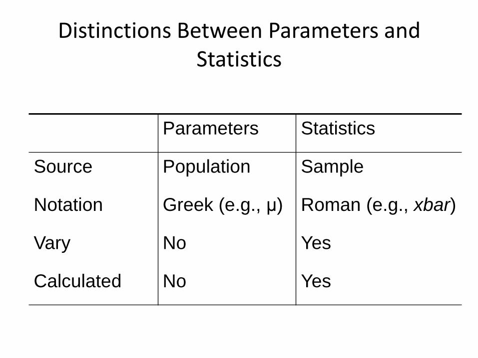
The statistician’s universe
Population Data
Params
Stats
Sample
Statistics
Approximate
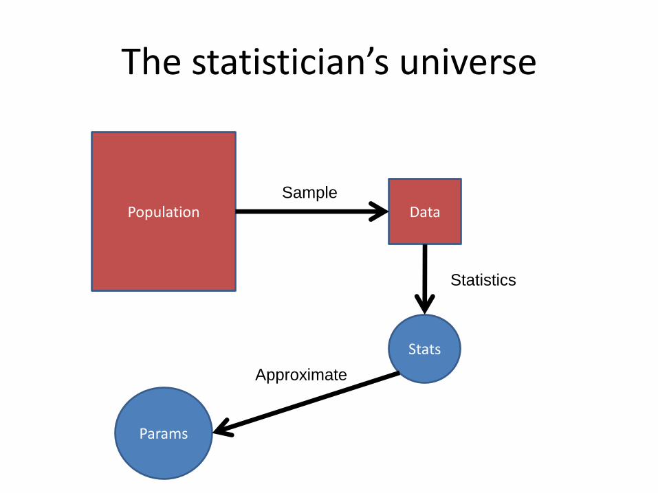
“The Reverend Bayes published posthumously. The field of statistics
would greatly improve if all Bayesians were to follow his example”

Sampling Distributions of a Mean
nSE
SENx
x
x
where
,~
The sampling distributions of a mean (SDM) describes the behavior of a sampling mean
Hypothesis Testing
• Is also called significance testing
• Tests a claim about a parameter using evidence (data in a sample
• The technique is introduced by considering a one-sample z test
• The procedure is broken into four steps
• Each element of the procedure must be understood

Hypothesis Testing Steps
A. Null and alternative hypotheses
B. Test statistic
C. P-value and interpretation
D. Significance level (optional)
Null and Alternative Hypotheses
• Convert the research question to null and alternative hypotheses
• The null hypothesis (H0) is a claim of “no difference in the population”
• The alternative hypothesis (Ha) claims “H0 is false”
• Collect data and seek evidence against H0 as a way of bolstering Ha (deduction)

Illustrative Example: “Body Weight”
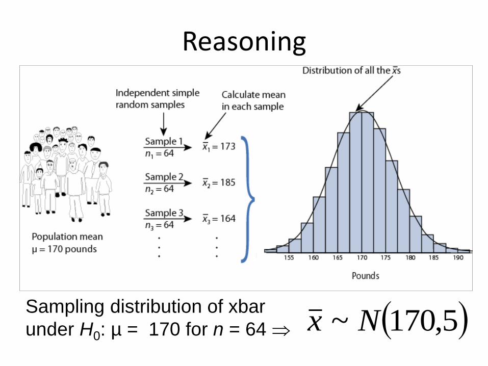
Reasoning
5,170~ NxSampling distribution of xbar
under H0: µ = 170 for n = 64

Test Statistic
nSE
H
SE
x
x
x
and
trueis assumingmean population where
z
00
0stat
This is an example of a one-sample test of a
mean when σ is known. Use this statistic to
test the problem:
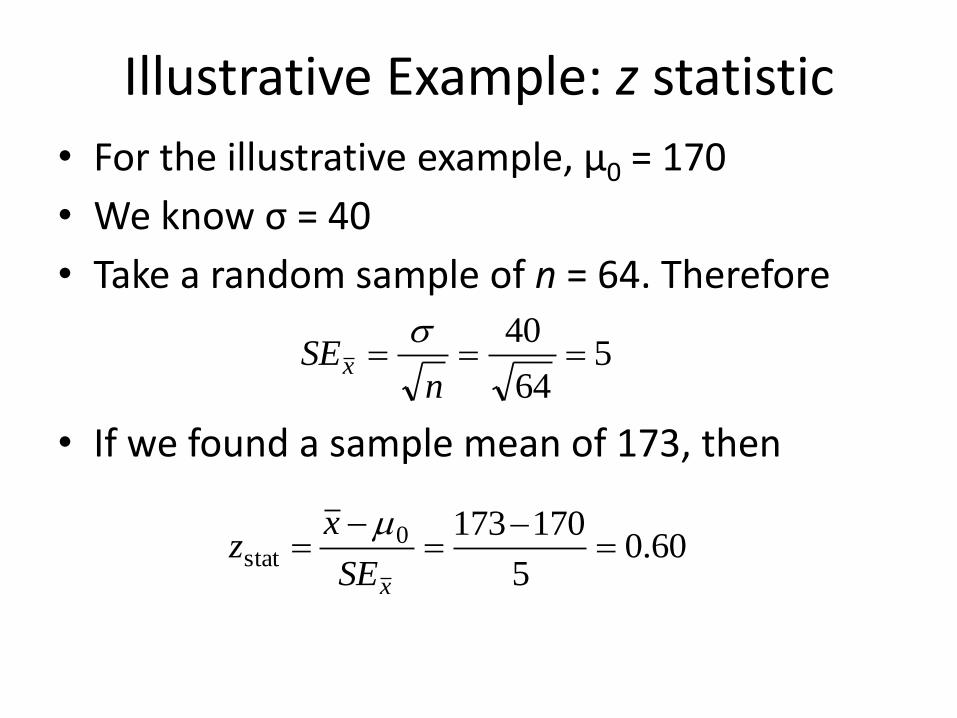
Illustrative Example: z statistic
• For the illustrative example, μ0 = 170
• We know σ = 40
• Take a random sample of n = 64. Therefore
• If we found a sample mean of 173, then
564
40
nSEx
60.05
170173 0
stat
xSE
xz

Illustrative Example: z statistic
If we found a sample mean of 185, then
00.35
170185 0
stat
xSE
xz
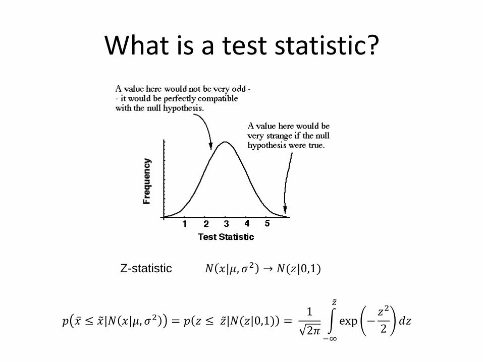
What is a test statistic?
𝑁 𝑥|𝜇, 𝜎2 → 𝑁(𝑧|0,1) Z-statistic
𝑝 𝑥 ≤ 𝑥 |𝑁 𝑥|𝜇, 𝜎2 = 𝑝 𝑧 ≤ 𝑧 |𝑁(𝑧|0,1) = 1
2𝜋 exp −
𝑧2
2𝑑𝑧
𝑧
−∞


p-value • The P-value answer the question: What is the
probability of the observed test statistic or one more extreme when H0 is true?
• This corresponds to the AUC in the tail of the Standard Normal distribution beyond the zstat.
• Convert z statistics to P-value : For Ha: μ > μ0 P = Pr(Z > zstat) = right-tail beyond zstat
For Ha: μ < μ0 P = Pr(Z < zstat) = left tail beyond zstat
For Ha: μ μ0 P = 2 × one-tailed P-value
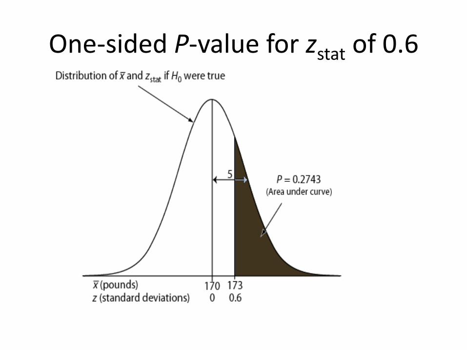
One-sided P-value for zstat of 0.6

One-sided P-value for zstat of 3.0

Two-Sided P-Value
• One-sided Ha AUC in tail beyond zstat
• Two-sided Ha consider potential deviations in both directions double the one-sided P-value
Examples: If one-sided P
= 0.0010, then two-sided
P = 2 × 0.0010 = 0.0020.
If one-sided P = 0.2743,
then two-sided P = 2 ×
0.2743 = 0.5486.

Interpretation
• P-value answer the question: What is the probability of the observed test statistic … when H0 is true?
• Thus, smaller and smaller P-values provide stronger and stronger evidence against H0
• Small P-value strong evidence

α-Level (Used in some situations)
• Let α ≡ probability of erroneously rejecting H0
• Set α threshold (e.g., let α = .10, .05, or whatever)
• Reject H0 when P ≤ α
• Retain H0 when P > α
• Example: Set α = .10. Find P = 0.27 retain H0
• Example: Set α = .01. Find P = .001 reject H0

(Summary) One-Sample z Test
A. Hypothesis statements H0: µ = µ0 vs. Ha: µ ≠ µ0 (two-sided) or Ha: µ < µ0 (left-sided) or Ha: µ > µ0 (right-sided)
B. Test statistic
C. P-value: convert z to p value
D. Significance statement depending on α
nSE
SE
xx
x
where z 0
stat
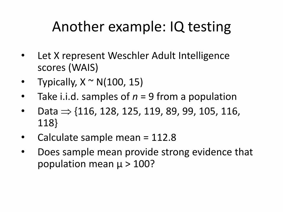
Another example: IQ testing
• Let X represent Weschler Adult Intelligence scores (WAIS)
• Typically, X ~ N(100, 15)
• Take i.i.d. samples of n = 9 from a population
• Data {116, 128, 125, 119, 89, 99, 105, 116, 118}
• Calculate sample mean = 112.8
• Does sample mean provide strong evidence that population mean μ > 100?
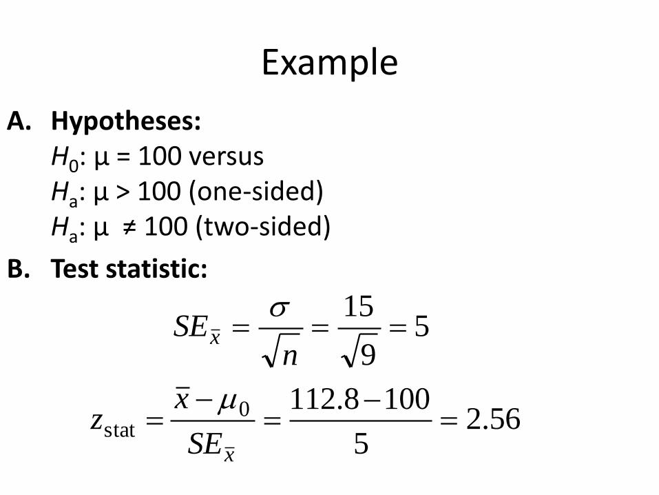
Example
56.25
1008.112
59
15
0stat
x
x
SE
xz
nSE
A. Hypotheses: H0: µ = 100 versus Ha: µ > 100 (one-sided) Ha: µ ≠ 100 (two-sided)
B. Test statistic:
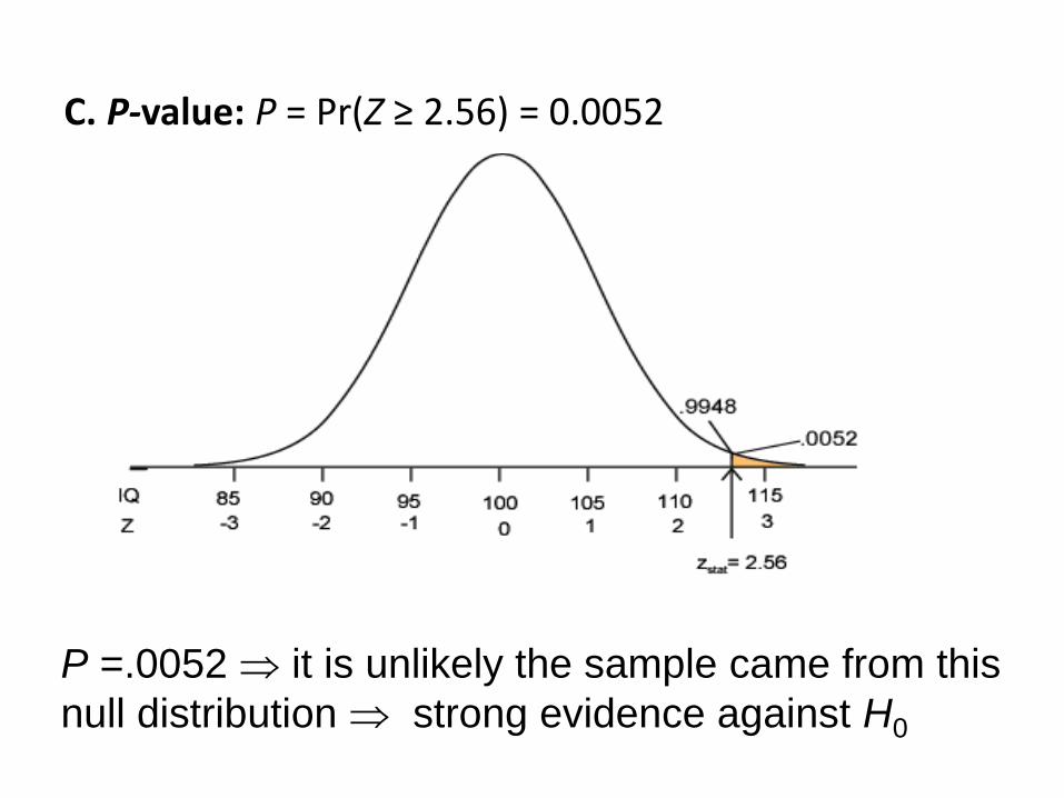
C. P-value: P = Pr(Z ≥ 2.56) = 0.0052
P =.0052 it is unlikely the sample came from this
null distribution strong evidence against H0
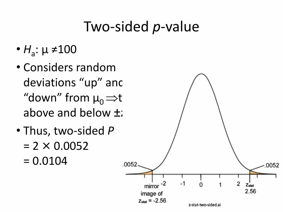
Two-sided p-value
• Ha: µ ≠100
• Considers random deviations “up” and “down” from μ0 tails above and below ±zstat
• Thus, two-sided P = 2 × 0.0052 = 0.0104

Conditions for z test
• σ known (not from data)
• Population approximately normal or large sample (n>30)
• Data i.i.d.
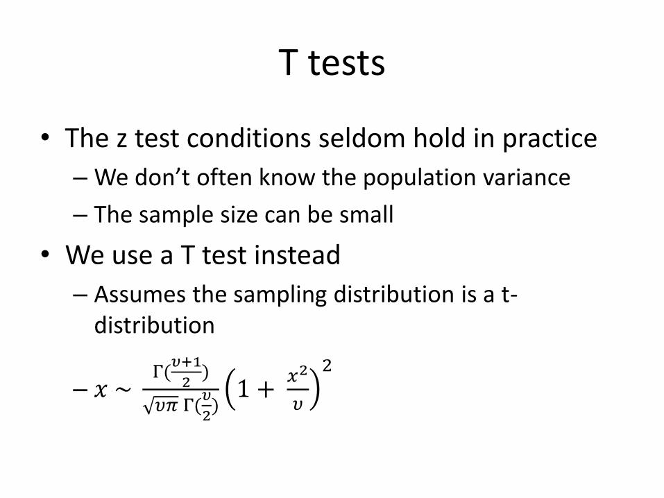
T tests
• The z test conditions seldom hold in practice
– We don’t often know the population variance
– The sample size can be small
• We use a T test instead
– Assumes the sampling distribution is a t-distribution
– 𝑥 ~ Γ(
𝜐+1
2)
𝜐𝜋 Γ(𝜐
2)
1 + 𝑥2
𝜐
2
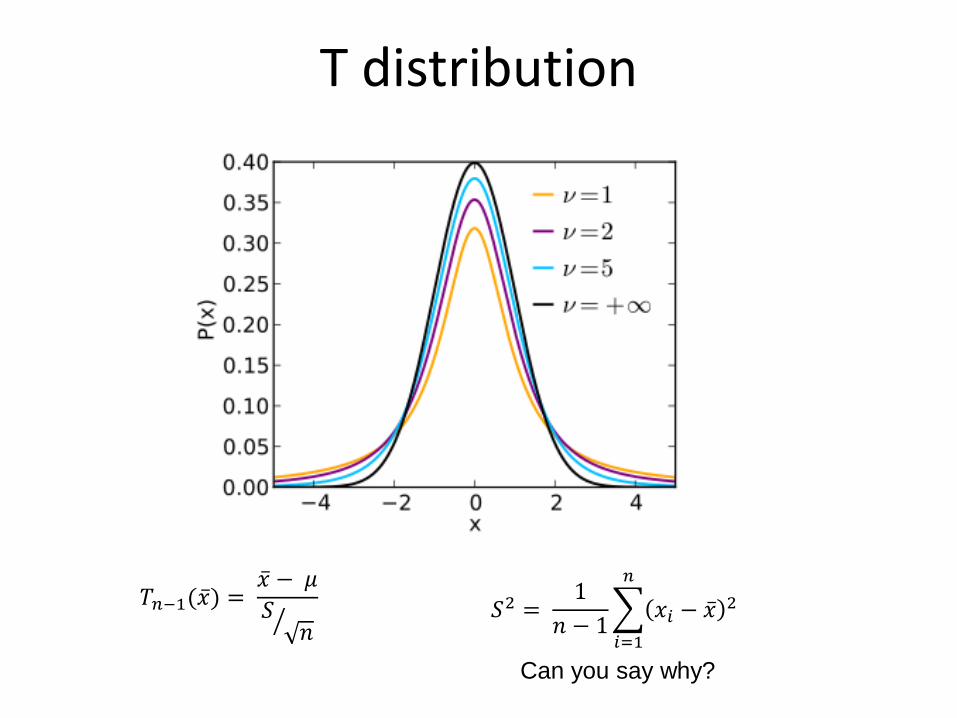
T distribution
𝑇𝑛−1(𝑥 ) = 𝑥 − 𝜇
𝑆𝑛
𝑆2 =
1
𝑛 − 1 𝑥𝑖 − 𝑥 2
𝑛
𝑖=1
Can you say why?

(Summary) T Test
A. Hypothesis statements H0: µ = µ0 vs. Ha: µ ≠ µ0 (two-sided) or Ha: µ < µ0 (left-sided) or Ha: µ > µ0 (right-sided)
B. Calculate Test statistic
C. P-value: convert T to p value
D. Significance statement depending on α
𝑇𝑛−1(𝑥 ) = 𝑥 − 𝜇
𝑆𝑛
𝑆2 = 1
𝑛 − 1 𝑥𝑖 − 𝑥 2
𝑛
𝑖=1
where,

Test statistics
Pooled
Unpooled

Test statistic construction
• Proportions as random variables
• What does the sampling distribution of the mean look like?
• What will the test statistic look like?
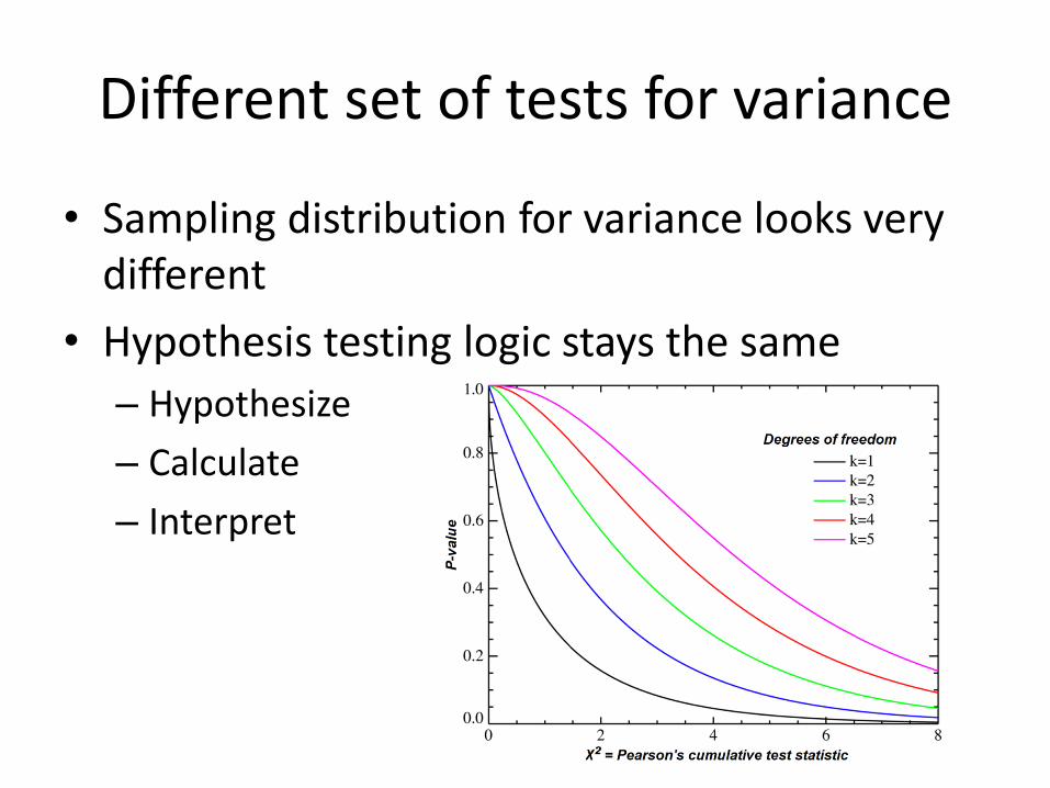
Different set of tests for variance
• Sampling distribution for variance looks very different
• Hypothesis testing logic stays the same
– Hypothesize
– Calculate
– Interpret
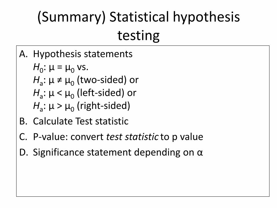
(Summary) Statistical hypothesis testing
A. Hypothesis statements H0: µ = µ0 vs. Ha: µ ≠ µ0 (two-sided) or Ha: µ < µ0 (left-sided) or Ha: µ > µ0 (right-sided)
B. Calculate Test statistic
C. P-value: convert test statistic to p value
D. Significance statement depending on α

PRACTICAL CONSIDERATIONS

Multiple comparisons
• Let’s say we’re doing IQ testing department-wise – 7 departments
– α = 0.05
– Run C(7,2) = 21 pairwise T-tests on the data
– CSE > EE
• How to interpret?
• Bonferroni correction for FWER α* = α/#comparisons

P-hacking

Reading error bars

Reading error bars
Use SD when you want to describe the dataset
Use SE when you want to describe the precision of your estimate of the mean
Use CI when your SE is small enough for the CI to look impressive to the
viewer!
Use of CI is strongly encouraged to report estimate precision. Be brave and use it

Confidence intervals
• Statistical estimates of population parameters are typically presented with confidence intervals
• 95% 𝐶𝐼 = 𝑍(𝑝 =0.05) × 𝑆𝐸
• Half the CI is sometimes called the margin of error
• How to set up data collection for a known margin of error?

Sample size calculation: simple
• Simplest case: one sample Z test
• Assume we want to find the population mean with margin of error at most W
• p = 0.05
• Then we want a CI of 2W and an SE of about W
• 𝑊 = 𝜎
𝑛, solve for n
• 𝑛 = 𝜎2
𝑊2
Cool trick: bootstrapping
• Power calculations depend on knowing the population standard deviation – Fine for Z tests, but what about the others?
• We use bootstrapping to estimate the population standard deviation from the data – Resample the data by drawing a dataset from the existing
dataset randomly with replacement – Compute statistics – Repeat 1000 times – You get an empirical distribution on the statistic – Directly use the standard deviation of this distribution as
the standard error of the statistic

Is this enough?
• Set up competing hypotheses
• Specify significance level
• Calculate confidence bound for test statistic – Use bootstrap if population variance is unknown
• Calculate effective sample size
• Collect data
• Calculate test statistic
• Output result

Not enough

Power
Truth
Decision H0 true H0 false
Retain H0 Correct retention Type II error
Reject H0 Type I error Correct rejection
α ≡ probability of a Type I error
β ≡ Probability of a Type II error
Two types of decision errors:
Type I error (FN) = erroneous rejection of true H0
Type II error (FP) = erroneous retention of false H0

Power • β ≡ probability of a Type II error
β = Pr(retain H0 | H0 false)
• 1 – β “Power” ≡ probability of avoiding a Type II error
1– β = Pr(reject H0 | H0 false)

Power calculation
21
z
1z
with
.
• Calculate probability of a Type II error – Pr(null is not rejected|null is false)
– 𝑝 𝑧 < 𝑧𝑐𝑟𝑖𝑡 𝑧 = 𝑥 − 𝜇1𝜎
𝑛 , 𝑥~𝑁(𝜇1, 𝜎))
– Power is 1 – p(Type II error)
• Calculate 𝑥𝑐𝑟𝑖𝑡 = 𝜇0 + 𝑧𝑐𝑟𝑖𝑡 𝜎
𝑛
– Power = 𝑝 𝑥 > 𝑥𝑐𝑟𝑖𝑡 𝑥~𝑁(𝜇1, 𝜎))
– Power = 𝑝 𝑧 ≥ 𝑥𝑐𝑟𝑖𝑡− 𝜇1
𝜎𝑛
= 1 − Φ(𝑥𝑐𝑟𝑖𝑡− 𝜇1
𝜎𝑛
)

Calculating Power: Example A study of n = 16 retains H0: μ = 170 at α = 0.05
(two-sided); σ is 40. What is the power of test’s
conditions to identify a population mean of 190?
𝑥𝑐𝑟𝑖𝑡 = 170 + 1.96 ×40
16= 189.6
𝑃𝑜𝑤𝑒𝑟 = 1 − Φ −0.04 = 0.5160
Can you find the power if we used 100 samples instead?
𝑥𝑐𝑟𝑖𝑡 = 170 + 1.96 ×40
100= 177.68
𝑃𝑜𝑤𝑒𝑟 = 1 − Φ −3.08 = 0.999


Illustration: conditions
for 90% power.

Effect size
• Frequently measured using Cohen’s d
• 𝑑 = 𝜇1−𝜇0
𝑠
• Bigger effect sizes easier to discriminate
• Estimate via pilots

Summary of statistical calculations
• Given any 3 of α, β, d and n, we can calculate the fourth
– Can calculate expected margin of error a test
– Can calculate expected power of a test
– Can calculate minimum discriminable effect size of a test
– Can calculate required sample size of a test
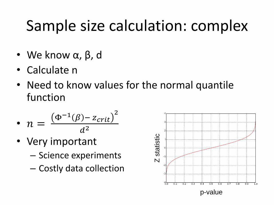
Sample size calculation: complex
• We know α, β, d
• Calculate n
• Need to know values for the normal quantile function
• 𝑛 = Φ−1 𝛽 − 𝑧𝑐𝑟𝑖𝑡
2
𝑑2
• Very important – Science experiments
– Costly data collection
p-value
Z s
tatistic

Review: statistics
• The language of statistics – Describes a universe where we sample datasets from
a population
• Interesting properties are proved for sampling distributions of parameter estimates
• Statistical hypothesis testing – Helps us decide if a sample belongs to a population
• A priori calculation of important statistical properties can help design better studies – Power, sample size, effect size
Top Related