Usage of Cohesive Elements in Crash Analysis of Large ... · Large, Bonded Vehicle Structures...
20
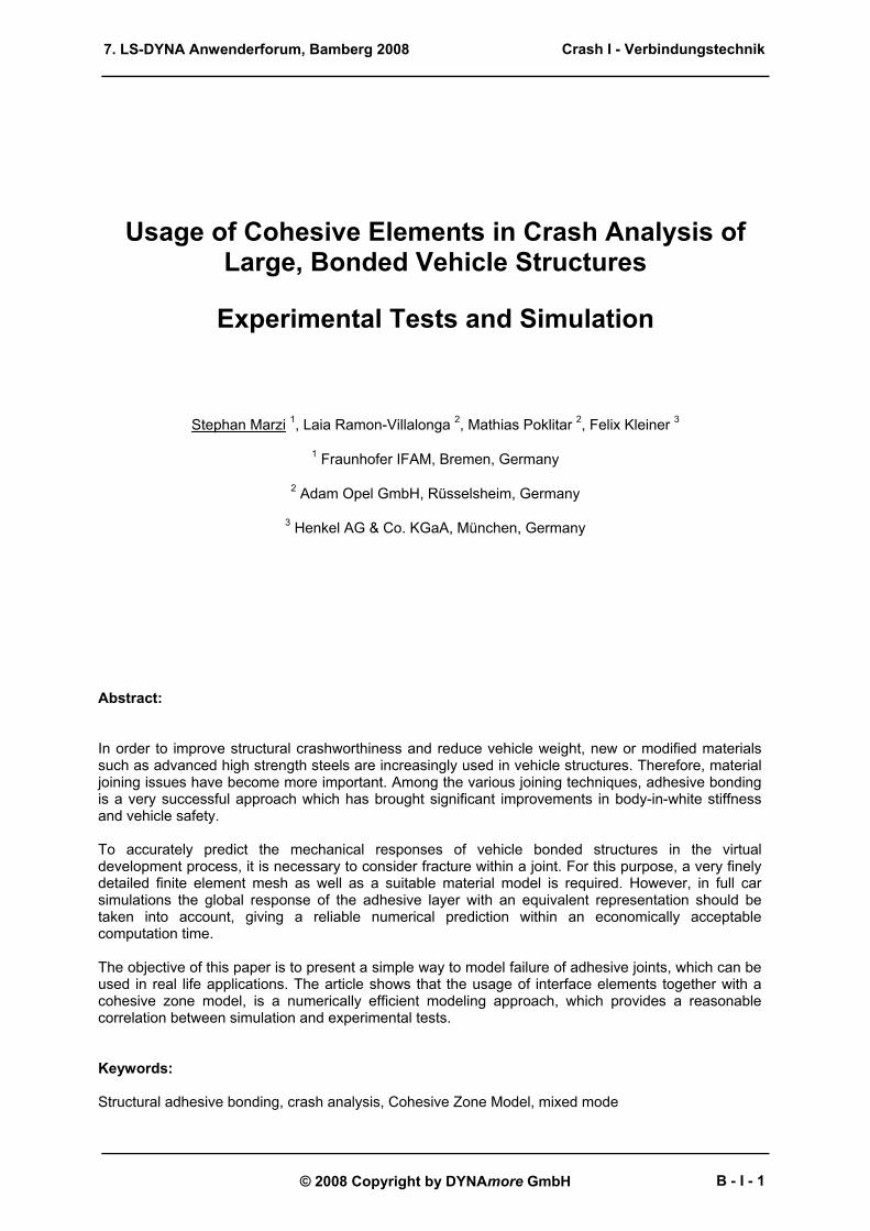
7. LS-DYNA Anwenderforum, Bamberg 2008 © 2008 Copyright by DYNAmore GmbH Usage of Cohesive Elements in Crash Analysis of Large, Bonded Vehicle Structures Experimental Tests and Simulation Stephan Marzi 1 , Laia Ramon-Villalonga 2 , Mathias Poklitar 2 , Felix Kleiner 3 1 Fraunhofer IFAM, Bremen, Germany 2 Adam Opel GmbH, Rüsselsheim, Germany 3 Henkel AG & Co. KGaA, München, Germany Abstract: In order to improve structural crashworthiness and reduce vehicle weight, new or modified materials such as advanced high strength steels are increasingly used in vehicle structures. Therefore, material joining issues have become more important. Among the various joining techniques, adhesive bonding is a very successful approach which has brought significant improvements in body-in-white stiffness and vehicle safety. To accurately predict the mechanical responses of vehicle bonded structures in the virtual development process, it is necessary to consider fracture within a joint. For this purpose, a very finely detailed finite element mesh as well as a suitable material model is required. However, in full car simulations the global response of the adhesive layer with an equivalent representation should be taken into account, giving a reliable numerical prediction within an economically acceptable computation time. The objective of this paper is to present a simple way to model failure of adhesive joints, which can be used in real life applications. The article shows that the usage of interface elements together with a cohesive zone model, is a numerically efficient modeling approach, which provides a reasonable correlation between simulation and experimental tests. Keywords: Structural adhesive bonding, crash analysis, Cohesive Zone Model, mixed mode Crash I - Verbindungstechnik B - I - 1
Transcript of Usage of Cohesive Elements in Crash Analysis of Large ... · Large, Bonded Vehicle Structures...
7. LS-DYNA Anwenderforum, Bamberg 2008
© 2008 Copyright by DYNAmore GmbH
Usage of Cohesive Elements in Crash Analysis of Large, Bonded Vehicle Structures
Experimental Tests and Simulation
Stephan Marzi 1, Laia Ramon-Villalonga 2, Mathias Poklitar 2, Felix Kleiner 3
1 Fraunhofer IFAM, Bremen, Germany
2 Adam Opel GmbH, Rüsselsheim, Germany
3 Henkel AG & Co. KGaA, München, Germany
Abstract: In order to improve structural crashworthiness and reduce vehicle weight, new or modified materials such as advanced high strength steels are increasingly used in vehicle structures. Therefore, material joining issues have become more important. Among the various joining techniques, adhesive bonding is a very successful approach which has brought significant improvements in body-in-white stiffness and vehicle safety. To accurately predict the mechanical responses of vehicle bonded structures in the virtual development process, it is necessary to consider fracture within a joint. For this purpose, a very finelydetailed finite element mesh as well as a suitable material model is required. However, in full car simulations the global response of the adhesive layer with an equivalent representation should be taken into account, giving a reliable numerical prediction within an economically acceptable computation time. The objective of this paper is to present a simple way to model failure of adhesive joints, which can be used in real life applications. The article shows that the usage of interface elements together with a cohesive zone model, is a numerically efficient modeling approach, which provides a reasonable correlation between simulation and experimental tests. Keywords: Structural adhesive bonding, crash analysis, Cohesive Zone Model, mixed mode
Crash I - Verbindungstechnik
B - I - 1
7. LS-DYNA Anwenderforum, Bamberg 2008
© 2008 Copyright by DYNAmore GmbH
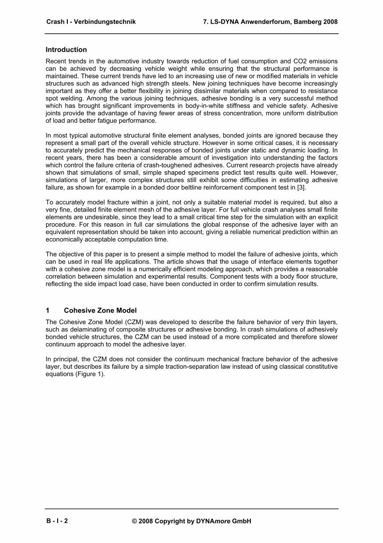
Introduction Recent trends in the automotive industry towards reduction of fuel consumption and CO2 emissions can be achieved by decreasing vehicle weight while ensuring that the structural performance is maintained. These current trends have led to an increasing use of new or modified materials in vehicle structures such as advanced high strength steels. New joining techniques have become increasingly important as they offer a better flexibility in joining dissimilar materials when compared to resistance spot welding. Among the various joining techniques, adhesive bonding is a very successful method which has brought significant improvements in body-in-white stiffness and vehicle safety. Adhesive joints provide the advantage of having fewer areas of stress concentration, more uniform distribution of load and better fatigue performance. In most typical automotive structural finite element analyses, bonded joints are ignored because they represent a small part of the overall vehicle structure. However in some critical cases, it is necessary to accurately predict the mechanical responses of bonded joints under static and dynamic loading. In recent years, there has been a considerable amount of investigation into understanding the factors which control the failure criteria of crash-toughened adhesives. Current research projects have already shown that simulations of small, simple shaped specimens predict test results quite well. However, simulations of larger, more complex structures still exhibit some difficulties in estimating adhesive failure, as shown for example in a bonded door beltline reinforcement component test in [3]. To accurately model fracture within a joint, not only a suitable material model is required, but also a very fine, detailed finite element mesh of the adhesive layer. For full vehicle crash analyses small finite elements are undesirable, since they lead to a small critical time step for the simulation with an explicit procedure. For this reason in full car simulations the global response of the adhesive layer with an equivalent representation should be taken into account, giving a reliable numerical prediction within an economically acceptable computation time. The objective of this paper is to present a simple method to model the failure of adhesive joints, which can be used in real life applications. The article shows that the usage of interface elements together with a cohesive zone model is a numerically efficient modeling approach, which provides a reasonable correlation between simulation and experimental results. Component tests with a body floor structure, reflecting the side impact load case, have been conducted in order to confirm simulation results.
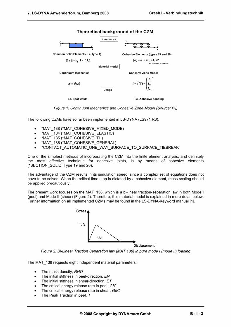
1 Cohesive Zone Model The Cohesive Zone Model (CZM) was developed to describe the failure behavior of very thin layers, such as delaminating of composite structures or adhesive bonding. In crash simulations of adhesively bonded vehicle structures, the CZM can be used instead of a more complicated and therefore slower continuum approach to model the adhesive layer. In principal, the CZM does not consider the continuum mechanical fracture behavior of the adhesive layer, but describes its failure by a simple traction-separation law instead of using classical constitutive equations (Figure 1).
Crash I - Verbindungstechnik
B - I - 2
7. LS-DYNA Anwenderforum, Bamberg 2008
© 2008 Copyright by DYNAmore GmbH
Theoretical background of the CZM
)(ˆ εσσ =
Kinematics
Common Solid Elements (i.e. type 1) Cohesive Elements (types 19 and 20)
[[ ε ]] = εij , i = 1,2,3 [δ ] = δi , i = t, s1, s2t = traction, s = shear
Material model
Continuum Mechanics
==
2
1)(ˆ
s
s
t
ttt
tt δ
Cohesive Zone Model
Usage
i.e. Spot welds i.e. Adhesive bonding
Figure 1: Continuum Mechanics and Cohesive Zone Model (Source: [3])
The following CZMs have so far been implemented in LS-DYNA (LS971 R3):
• *MAT_138 (*MAT_COHESIVE_MIXED_MODE) • *MAT_184 (*MAT_COHESIVE_ELASTIC) • *MAT_185 (*MAT_COHESIVE_TH) • *MAT_186 (*MAT_COHESIVE_GENERAL) • *CONTACT_AUTOMATIC_ONE_WAY_SURFACE_TO_SURFACE_TIEBREAK
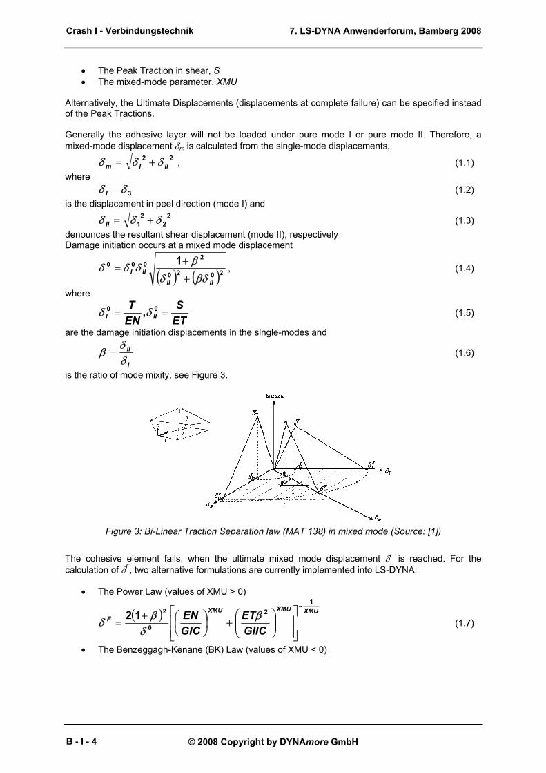
One of the simplest methods of incorporating the CZM into the finite element analysis, and definitely the most effective technique for adhesive joints, is by means of cohesive elements (*SECTION_SOLID, Type 19 and 20). The advantage of the CZM results in its simulation speed, since a complex set of equations does not have to be solved. When the critical time step is dictated by a cohesive element, mass scaling should be applied precautiously. The present work focuses on the MAT_138, which is a bi-linear traction-separation law in both Mode I (peel) and Mode II (shear) (Figure 2). Therefore, this material model is explained in more detail below. Further information on all implemented CZMs may be found in the LS-DYNA-Keyword manual [1].
Displacement
Stress
GC
T, S
Displacement
Stress
GC
T, S
Figure 2: Bi-Linear Traction Separation law (MAT 138) in pure mode I (mode II) loading
The MAT_138 requests eight independent material parameters:
• The mass density, RHO • The initial stiffness in peel-direction, EN • The initial stiffness in shear-direction, ET • The critical energy release rate in peel, GIC • The critical energy release rate in shear, GIIC • The Peak Traction in peel, T
Crash I - Verbindungstechnik
B - I - 3
7. LS-DYNA Anwenderforum, Bamberg 2008
© 2008 Copyright by DYNAmore GmbH
• The Peak Traction in shear, S • The mixed-mode parameter, XMU
Alternatively, the Ultimate Displacements (displacements at complete failure) can be specified instead of the Peak Tractions. Generally the adhesive layer will not be loaded under pure mode I or pure mode II. Therefore, a mixed-mode displacement δm is calculated from the single-mode displacements,
22IIIm δδδ += , (1.1)
where
3δδ =I (1.2) is the displacement in peel direction (mode I) and
22
21 δδδ +=II (1.3)
denounces the resultant shear displacement (mode II), respectively Damage initiation occurs at a mixed mode displacement
( ) ( )2020
2000 1
IIIIIII
βδδ
βδδδ+
+= , (1.4)
where
ETS
ENT
III == 00 ,δδ (1.5)
are the damage initiation displacements in the single-modes and
I
II
δδ
β = (1.6)
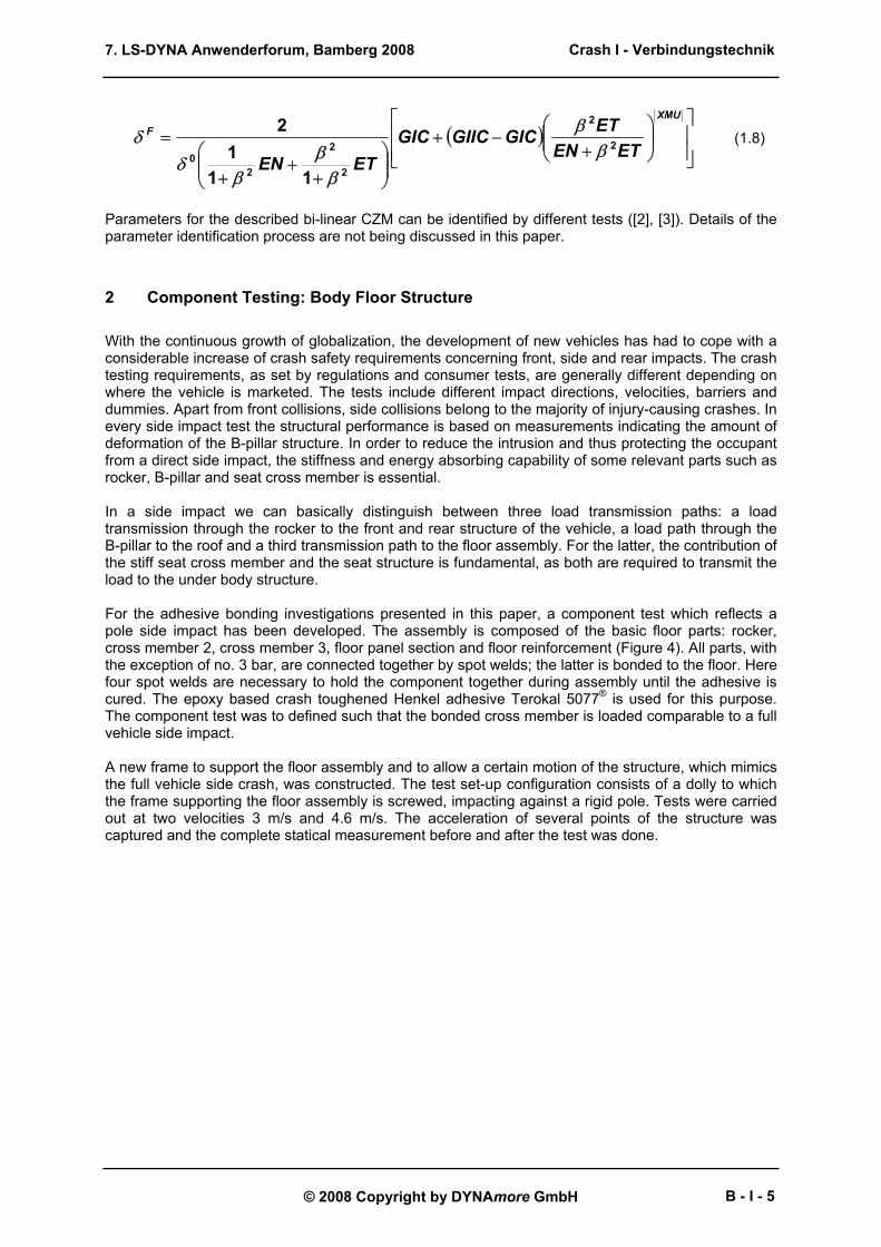
is the ratio of mode mixity, see Figure 3.
Figure 3: Bi-Linear Traction Separation law (MAT 138) in mixed mode (Source: [1])
The cohesive element fails, when the ultimate mixed mode displacement δF is reached. For the calculation of δF, two alternative formulations are currently implemented into LS-DYNA:
• The Power Law (values of XMU > 0)
( ) XMUXMUXMUF
GIICET
GICEN
12
0
212−
+
+
=β
δβδ (1.7)
• The Benzeggagh-Kenane (BK) Law (values of XMU < 0)
Crash I - Verbindungstechnik
B - I - 4
7. LS-DYNA Anwenderforum, Bamberg 2008
© 2008 Copyright by DYNAmore GmbH
( )
+
−+
+
++
=XMU
F
ETENETGICGIICGIC
ETEN2
2
2
2
20
111
2β
β
ββ
βδ
δ (1.8)
Parameters for the described bi-linear CZM can be identified by different tests ([2], [3]). Details of the parameter identification process are not being discussed in this paper.
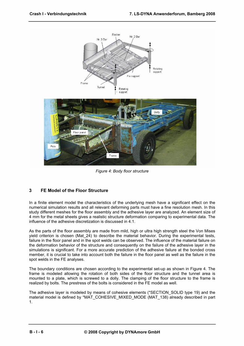
2 Component Testing: Body Floor Structure With the continuous growth of globalization, the development of new vehicles has had to cope with a considerable increase of crash safety requirements concerning front, side and rear impacts. The crash testing requirements, as set by regulations and consumer tests, are generally different depending on where the vehicle is marketed. The tests include different impact directions, velocities, barriers and dummies. Apart from front collisions, side collisions belong to the majority of injury-causing crashes. In every side impact test the structural performance is based on measurements indicating the amount of deformation of the B-pillar structure. In order to reduce the intrusion and thus protecting the occupant from a direct side impact, the stiffness and energy absorbing capability of some relevant parts such as rocker, B-pillar and seat cross member is essential. In a side impact we can basically distinguish between three load transmission paths: a load transmission through the rocker to the front and rear structure of the vehicle, a load path through the B-pillar to the roof and a third transmission path to the floor assembly. For the latter, the contribution of the stiff seat cross member and the seat structure is fundamental, as both are required to transmit the load to the under body structure. For the adhesive bonding investigations presented in this paper, a component test which reflects a pole side impact has been developed. The assembly is composed of the basic floor parts: rocker, cross member 2, cross member 3, floor panel section and floor reinforcement (Figure 4). All parts, with the exception of no. 3 bar, are connected together by spot welds; the latter is bonded to the floor. Here four spot welds are necessary to hold the component together during assembly until the adhesive is cured. The epoxy based crash toughened Henkel adhesive Terokal 5077® is used for this purpose. The component test was to defined such that the bonded cross member is loaded comparable to a full vehicle side impact. A new frame to support the floor assembly and to allow a certain motion of the structure, which mimics the full vehicle side crash, was constructed. The test set-up configuration consists of a dolly to which the frame supporting the floor assembly is screwed, impacting against a rigid pole. Tests were carried out at two velocities 3 m/s and 4.6 m/s. The acceleration of several points of the structure was captured and the complete statical measurement before and after the test was done.
Crash I - Verbindungstechnik
B - I - 5
7. LS-DYNA Anwenderforum, Bamberg 2008
© 2008 Copyright by DYNAmore GmbH
Figure 4: Body floor structure
3 FE Model of the Floor Structure In a finite element model the characteristics of the underlying mesh have a significant effect on the numerical simulation results and all relevant deforming parts must have a fine resolution mesh. In this study different meshes for the floor assembly and the adhesive layer are analyzed. An element size of 4 mm for the metal sheets gives a realistic structure deformation comparing to experimental data. The influence of the adhesive discretization is discussed in 4.1. As the parts of the floor assembly are made from mild, high or ultra high strength steel the Von Mises yield criterion is chosen (Mat_24) to describe the material behavior. During the experimental tests, failure in the floor panel and in the spot welds can be observed. The influence of the material failure on the deformation behavior of the structure and consequently on the failure of the adhesive layer in the simulations is significant. For a more accurate prediction of the adhesive failure at the bonded cross member, it is crucial to take into account both the failure in the floor panel as well as the failure in the spot welds in the FE analyses. The boundary conditions are chosen according to the experimental set-up as shown in Figure 4. The frame is modeled allowing the rotation of both sides of the floor structure and the tunnel area is mounted to a plate, which is screwed to a dolly. The clamping of the floor structure to the frame is realized by bolts. The prestress of the bolts is considered in the FE model as well. The adhesive layer is modeled by means of cohesive elements (*SECTION_SOLID type 19) and the material model is defined by *MAT_COHESIVE_MIXED_MODE (MAT_138) already described in part 1.
Crash I - Verbindungstechnik
B - I - 6
7. LS-DYNA Anwenderforum, Bamberg 2008
© 2008 Copyright by DYNAmore GmbH
4 Adhesive Modeling In a finite element crash analysis the adhesive layer can be modeled in different ways: using mesh dependent methods, which means modeling common nodes between solids and shells, or using mesh independent methods. A congruent connection between adhesive and adherents may result in either a very coarse mesh for the adhesive layer, or a very fine mesh for the adherents. Alternatively the adhesive layer can be connected by an incongruent mesh to the adherents, i.e. using the *CONTACT_TIED_NODES_TO_SURFACE option in LS-DYNA. When choosing this solution it has to be clarified, how the element size of the adhesive layer influences the failure behavior of the modeled joint and the total structure. In this chapter, different adherent and adhesive discretizations are compared to each other. Since this chapter focuses on adhesive modeling, the four spot welds connecting the cross beam number three with the floor panel are not modeled. The presence of such spot welds could influence the failure behavior of the bonded part significantly. A velocity of 4.5 m/s for the floor assembly impacting against the pole was chosen in all simulations presented below. In industrial appliances, mass scaling is normally used to reduce the simulation time, but it may affect the simulation results. Therefore, the investigations on the influence of the adhesive modeling technique in chapter 4.1 are done in absence of mass scaling (no MS). Chapter 4.2 discusses the influences of mass scaling on the different investigated discretizations and its benefits to the simulation effort.
4.1 Influence of adhesive mesh technique
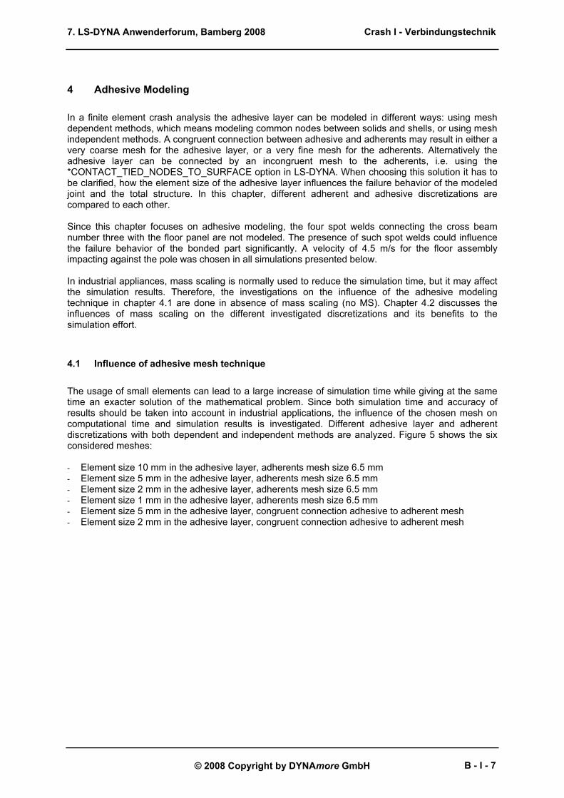
The usage of small elements can lead to a large increase of simulation time while giving at the same time an exacter solution of the mathematical problem. Since both simulation time and accuracy of results should be taken into account in industrial applications, the influence of the chosen mesh on computational time and simulation results is investigated. Different adhesive layer and adherent discretizations with both dependent and independent methods are analyzed. Figure 5 shows the six considered meshes: - Element size 10 mm in the adhesive layer, adherents mesh size 6.5 mm - Element size 5 mm in the adhesive layer, adherents mesh size 6.5 mm - Element size 2 mm in the adhesive layer, adherents mesh size 6.5 mm - Element size 1 mm in the adhesive layer, adherents mesh size 6.5 mm - Element size 5 mm in the adhesive layer, congruent connection adhesive to adherent mesh - Element size 2 mm in the adhesive layer, congruent connection adhesive to adherent mesh
Crash I - Verbindungstechnik
B - I - 7
7. LS-DYNA Anwenderforum, Bamberg 2008
© 2008 Copyright by DYNAmore GmbH
Figure 5: Considered meshes of the adhesive layer
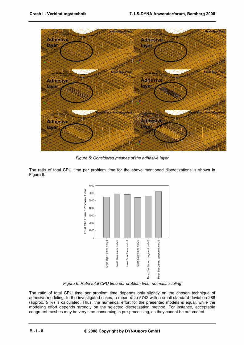
The ratio of total CPU time per problem time for the above mentioned discretizations is shown in Figure 6.
Mes
h si
ze 1
0 m
m, n
o M
S
Mes
h S
ize
5 m
m, n
o M
S
Mes
h S
ize
2 m
m, n
o M
S
Mes
h S
ize
1 m
m, n
o M
S
Mes
h Si
ze 5
mm
, con
grue
nt, n
o M
S
Mes
h Si
ze 2
mm
, con
grue
nt, n
o M
S
Tota
l CPU
tim
e / P
robl
em T
ime
0
1000
2000
3000
4000
5000
6000
7000
Figure 6: Ratio total CPU time per problem time, no mass scaling
The ratio of total CPU time per problem time depends only slightly on the chosen technique of adhesive modeling. In the investigated cases, a mean ratio 5742 with a small standard deviation 288 (approx. 5 %) is calculated. Thus, the numerical effort for the presented models is equal, while the modeling effort depends strongly on the selected discretization method. For instance, acceptable congruent meshes may be very time-consuming in pre-processing, as they cannot be automated.
Adhesive layer
Adhesive layer
Adhesive layer
Adhesive layer
Adhesive layer
Adhesive layer
Crash I - Verbindungstechnik
B - I - 8
7. LS-DYNA Anwenderforum, Bamberg 2008
© 2008 Copyright by DYNAmore GmbH
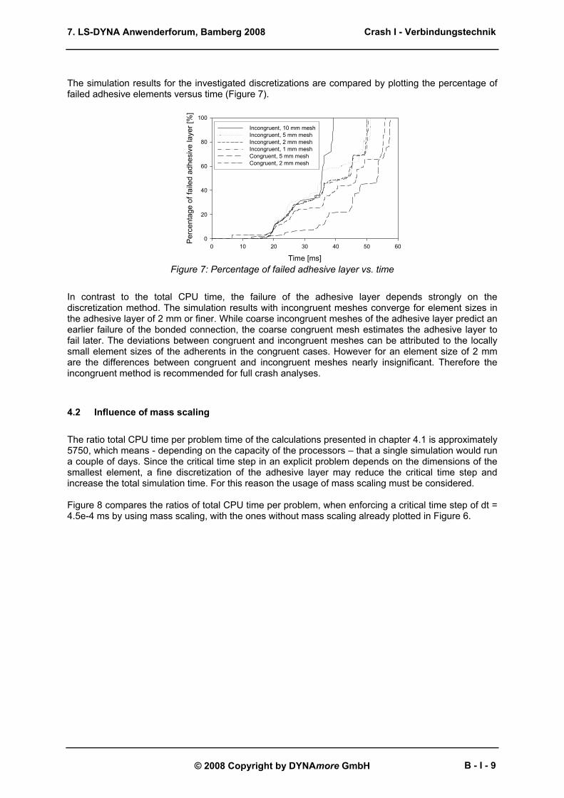
The simulation results for the investigated discretizations are compared by plotting the percentage of failed adhesive elements versus time (Figure 7).
Time [ms]0 10 20 30 40 50 60
Perc
enta
ge o
f fai
led
adhe
sive
laye
r [%
]
0
20
40
60
80
100
Incongruent, 10 mm meshIncongruent, 5 mm meshIncongruent, 2 mm meshIncongruent, 1 mm meshCongruent, 5 mm meshCongruent, 2 mm mesh
Figure 7: Percentage of failed adhesive layer vs. time
In contrast to the total CPU time, the failure of the adhesive layer depends strongly on the discretization method. The simulation results with incongruent meshes converge for element sizes in the adhesive layer of 2 mm or finer. While coarse incongruent meshes of the adhesive layer predict an earlier failure of the bonded connection, the coarse congruent mesh estimates the adhesive layer to fail later. The deviations between congruent and incongruent meshes can be attributed to the locally small element sizes of the adherents in the congruent cases. However for an element size of 2 mm are the differences between congruent and incongruent meshes nearly insignificant. Therefore the incongruent method is recommended for full crash analyses.
4.2 Influence of mass scaling
The ratio total CPU time per problem time of the calculations presented in chapter 4.1 is approximately 5750, which means - depending on the capacity of the processors – that a single simulation would run a couple of days. Since the critical time step in an explicit problem depends on the dimensions of the smallest element, a fine discretization of the adhesive layer may reduce the critical time step and increase the total simulation time. For this reason the usage of mass scaling must be considered. Figure 8 compares the ratios of total CPU time per problem, when enforcing a critical time step of dt = 4.5e-4 ms by using mass scaling, with the ones without mass scaling already plotted in Figure 6.
Crash I - Verbindungstechnik
B - I - 9
7. LS-DYNA Anwenderforum, Bamberg 2008
© 2008 Copyright by DYNAmore GmbH
Mes
h si
ze 1
0 m
m
Mes
h S
ize
5 m
m
Mes
h S
ize
2 m
m
Mes
h S
ize
1 m
m
Mes
h Si
ze 5
mm
, con
grue
nt
Mes
h Si
ze 2
mm
, con
grue
nt
Mes
h si
ze 1
0 m
m, n
o M
S
Mes
h S
ize
5 m
m, n
o M
S
Mes
h S
ize
2 m
m, n
o M
S
Mes
h S
ize
1 m
m, n
o M
S
Mes
h Si
ze 5
mm
, con
grue
nt, n
o M
S
Mes
h Si
ze 2
mm
, con
grue
nt, n
o M
S
Tota
l CPU
tim
e / P
robl
em T
ime
0
1000
2000
3000
4000
5000
6000
7000
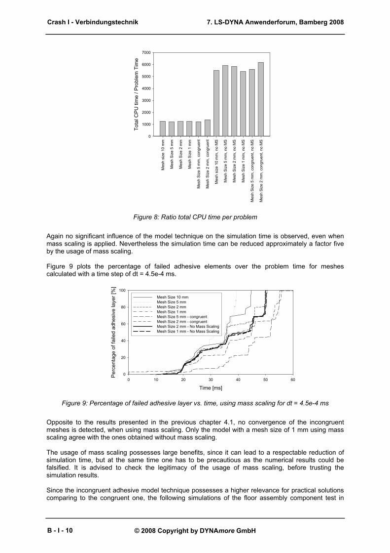
Figure 8: Ratio total CPU time per problem
Again no significant influence of the model technique on the simulation time is observed, even when mass scaling is applied. Nevertheless the simulation time can be reduced approximately a factor five by the usage of mass scaling. Figure 9 plots the percentage of failed adhesive elements over the problem time for meshes calculated with a time step of dt = 4.5e-4 ms.
Time [ms]0 10 20 30 40 50 60
Perc
enta
ge o
f fai
led
adhe
sive
laye
r [%
]
0
20
40
60
80
100
Mesh Size 10 mmMesh Size 5 mmMesh Size 2 mmMesh Size 1 mm Mesh Size 5 mm - congruentMesh Size 2 mm - congruentMesh Size 2 mm - No Mass ScalingMesh Size 1 mm - No Mass Scaling
Figure 9: Percentage of failed adhesive layer vs. time, using mass scaling for dt = 4.5e-4 ms
Opposite to the results presented in the previous chapter 4.1, no convergence of the incongruent meshes is detected, when using mass scaling. Only the model with a mesh size of 1 mm using mass scaling agree with the ones obtained without mass scaling. The usage of mass scaling possesses large benefits, since it can lead to a respectable reduction of simulation time, but at the same time one has to be precautious as the numerical results could be falsified. It is advised to check the legitimacy of the usage of mass scaling, before trusting the simulation results. Since the incongruent adhesive model technique possesses a higher relevance for practical solutions comparing to the congruent one, the following simulations of the floor assembly component test in
Crash I - Verbindungstechnik
B - I - 10
7. LS-DYNA Anwenderforum, Bamberg 2008
© 2008 Copyright by DYNAmore GmbH
chapter 5 are realized with an incongruent mesh. The mesh of the adhesive must have an element size of 1 mm to obtain consistent results, when mass scaling is applied, as discussed above.
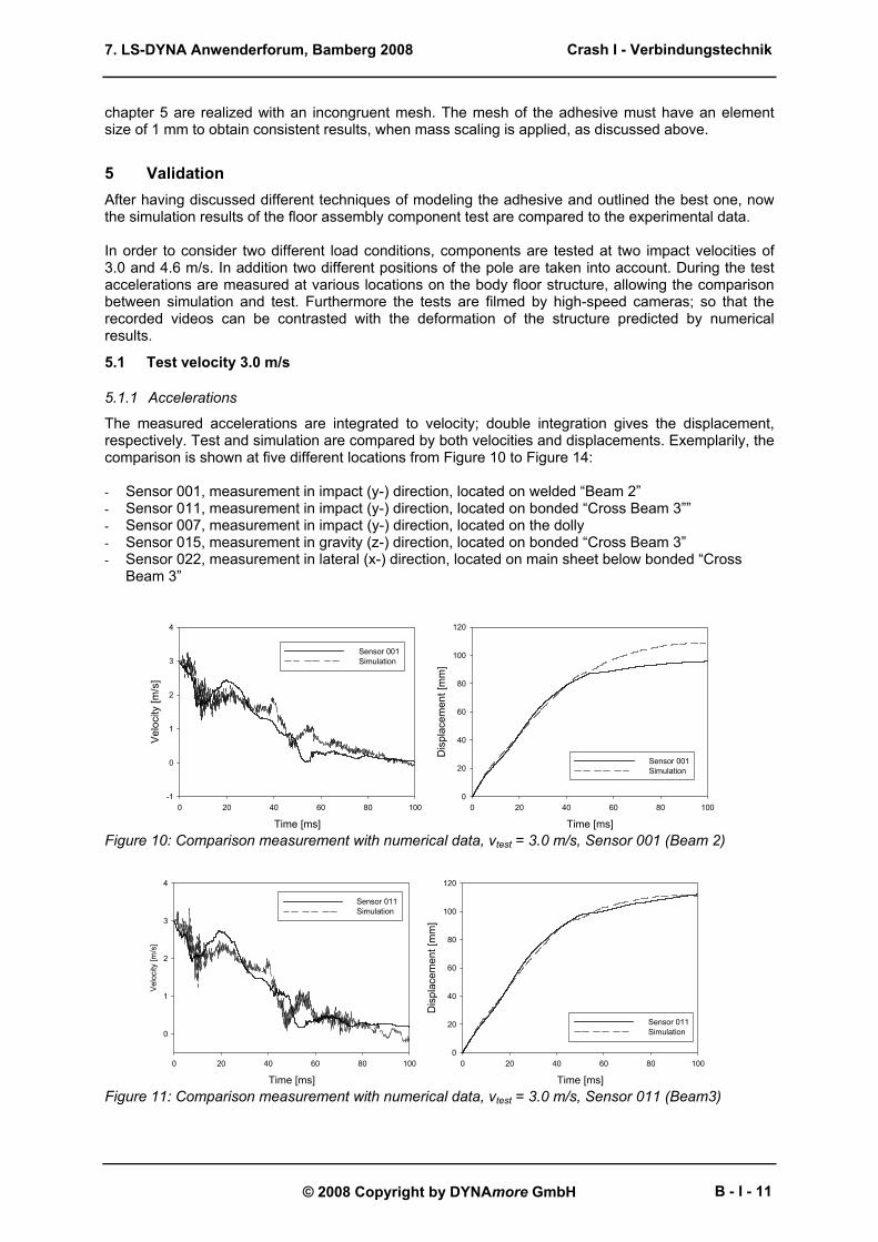
5 Validation After having discussed different techniques of modeling the adhesive and outlined the best one, now the simulation results of the floor assembly component test are compared to the experimental data. In order to consider two different load conditions, components are tested at two impact velocities of 3.0 and 4.6 m/s. In addition two different positions of the pole are taken into account. During the test accelerations are measured at various locations on the body floor structure, allowing the comparison between simulation and test. Furthermore the tests are filmed by high-speed cameras; so that the recorded videos can be contrasted with the deformation of the structure predicted by numerical results.
5.1 Test velocity 3.0 m/s
5.1.1 Accelerations
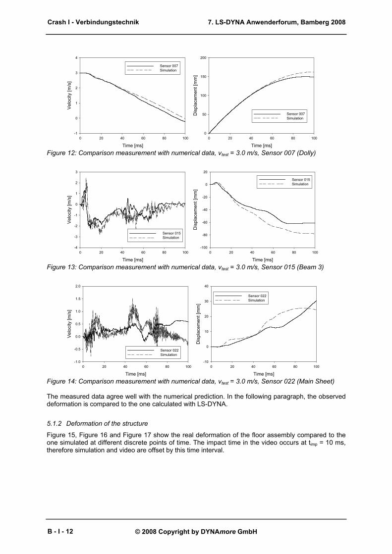
The measured accelerations are integrated to velocity; double integration gives the displacement, respectively. Test and simulation are compared by both velocities and displacements. Exemplarily, the comparison is shown at five different locations from Figure 10 to Figure 14: - Sensor 001, measurement in impact (y-) direction, located on welded “Beam 2” - Sensor 011, measurement in impact (y-) direction, located on bonded “Cross Beam 3”” - Sensor 007, measurement in impact (y-) direction, located on the dolly - Sensor 015, measurement in gravity (z-) direction, located on bonded “Cross Beam 3” - Sensor 022, measurement in lateral (x-) direction, located on main sheet below bonded “Cross
Beam 3”
Time [ms]0 20 40 60 80 100
Velo
city
[m/s
]
-1
0
1
2
3
4
Sensor 001Simulation
Time [ms]0 20 40 60 80 100
Dis
plac
emen
t [m
m]
0
20
40
60
80
100
120
Sensor 001Simulation
Figure 10: Comparison measurement with numerical data, vtest = 3.0 m/s, Sensor 001 (Beam 2)
Time [ms]0 20 40 60 80 100
Vel
ocity
[m/s
]
0
1
2
3
4
Sensor 011Simulation
Time [ms]0 20 40 60 80 100
Dis
plac
emen
t [m
m]
0
20
40
60
80
100
120
Sensor 011Simulation
Figure 11: Comparison measurement with numerical data, vtest = 3.0 m/s, Sensor 011 (Beam3)
Crash I - Verbindungstechnik
B - I - 11
7. LS-DYNA Anwenderforum, Bamberg 2008
© 2008 Copyright by DYNAmore GmbH
Time [ms]0 20 40 60 80 100
Velo
city
[m/s
]
-1
0
1
2
3
4
Sensor 007Simulation
Time [ms]0 20 40 60 80 100
Dis
plac
emen
t [m
m]
0
50
100
150
200
Sensor 007Simulation
Figure 12: Comparison measurement with numerical data, vtest = 3.0 m/s, Sensor 007 (Dolly)
Time [ms]0 20 40 60 80 100
Velo
city
[m/s
]
-4
-3
-2
-1
0
1
2
3
Sensor 015Simulation
Time [ms]0 20 40 60 80 100
Dis
plac
emen
t [m
m]
-100
-80
-60
-40
-20
0
20
Sensor 015Simulation
Figure 13: Comparison measurement with numerical data, vtest = 3.0 m/s, Sensor 015 (Beam 3)
Time [ms]0 20 40 60 80 100
Velo
city
[m/s
]
-1.0
-0.5
0.0
0.5
1.0
1.5
2.0
Sensor 022Simulation
Time [ms]0 20 40 60 80 100
Dis
plac
emen
t [m
m]
-10
0
10
20
30
40
Sensor 022Simulation
Figure 14: Comparison measurement with numerical data, vtest = 3.0 m/s, Sensor 022 (Main Sheet) The measured data agree well with the numerical prediction. In the following paragraph, the observed deformation is compared to the one calculated with LS-DYNA.
5.1.2 Deformation of the structure
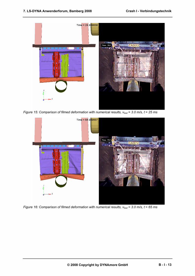
Figure 15, Figure 16 and Figure 17 show the real deformation of the floor assembly compared to the one simulated at different discrete points of time. The impact time in the video occurs at timp = 10 ms, therefore simulation and video are offset by this time interval.
Crash I - Verbindungstechnik
B - I - 12
7. LS-DYNA Anwenderforum, Bamberg 2008
© 2008 Copyright by DYNAmore GmbH
Figure 15: Comparison of filmed deformation with numerical results, vtest = 3.0 m/s, t = 25 ms
Figure 16: Comparison of filmed deformation with numerical results, vtest = 3.0 m/s, t = 65 ms
Crash I - Verbindungstechnik
B - I - 13
7. LS-DYNA Anwenderforum, Bamberg 2008
© 2008 Copyright by DYNAmore GmbH
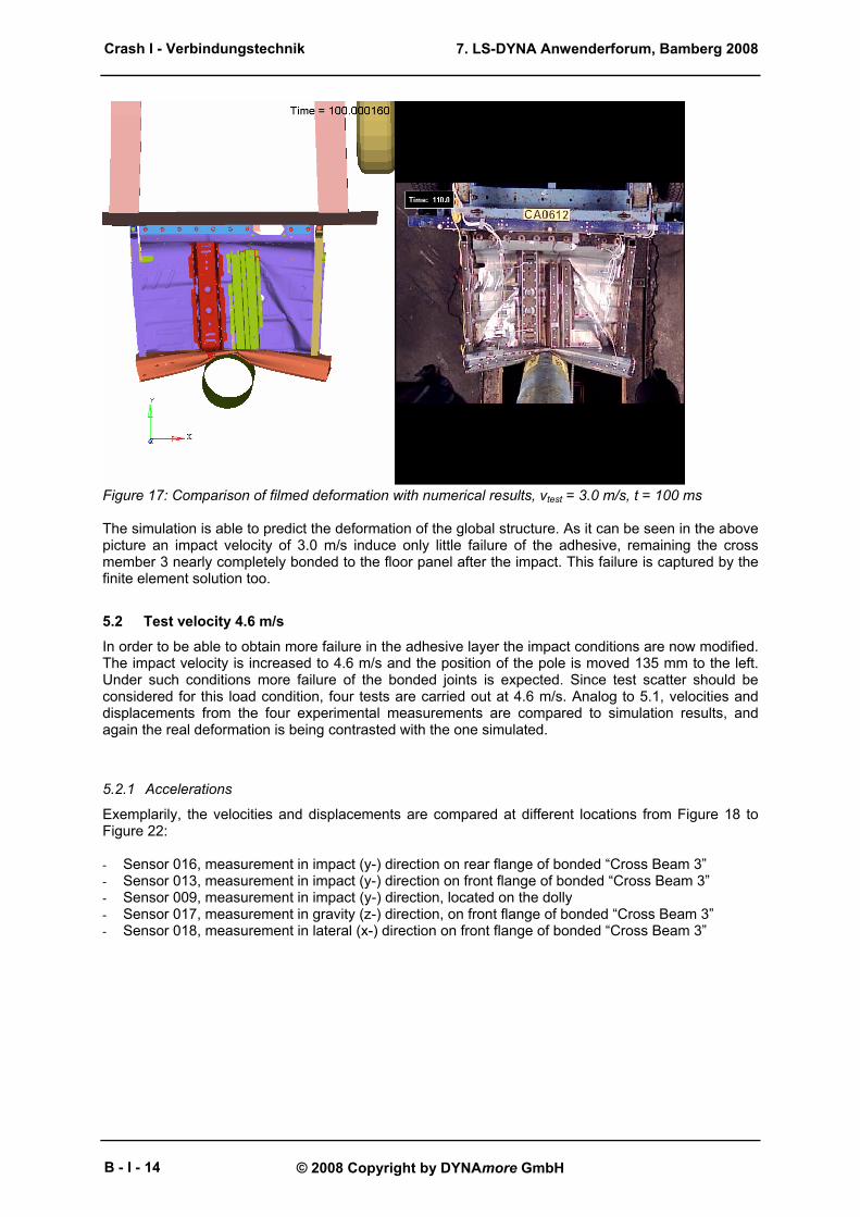
Figure 17: Comparison of filmed deformation with numerical results, vtest = 3.0 m/s, t = 100 ms The simulation is able to predict the deformation of the global structure. As it can be seen in the above picture an impact velocity of 3.0 m/s induce only little failure of the adhesive, remaining the cross member 3 nearly completely bonded to the floor panel after the impact. This failure is captured by the finite element solution too.
5.2 Test velocity 4.6 m/s
In order to be able to obtain more failure in the adhesive layer the impact conditions are now modified. The impact velocity is increased to 4.6 m/s and the position of the pole is moved 135 mm to the left. Under such conditions more failure of the bonded joints is expected. Since test scatter should be considered for this load condition, four tests are carried out at 4.6 m/s. Analog to 5.1, velocities and displacements from the four experimental measurements are compared to simulation results, and again the real deformation is being contrasted with the one simulated.
5.2.1 Accelerations
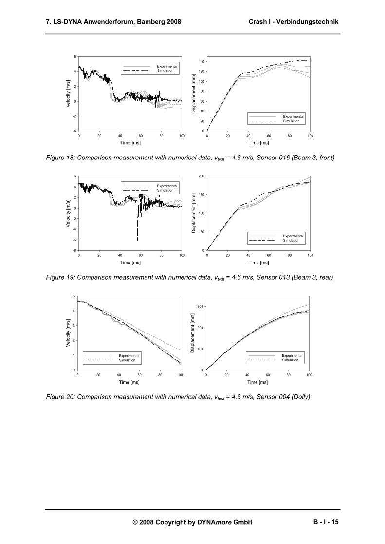
Exemplarily, the velocities and displacements are compared at different locations from Figure 18 to Figure 22: - Sensor 016, measurement in impact (y-) direction on rear flange of bonded “Cross Beam 3” - Sensor 013, measurement in impact (y-) direction on front flange of bonded “Cross Beam 3” - Sensor 009, measurement in impact (y-) direction, located on the dolly - Sensor 017, measurement in gravity (z-) direction, on front flange of bonded “Cross Beam 3” - Sensor 018, measurement in lateral (x-) direction on front flange of bonded “Cross Beam 3”
Crash I - Verbindungstechnik
B - I - 14
7. LS-DYNA Anwenderforum, Bamberg 2008
© 2008 Copyright by DYNAmore GmbH
Time [ms]0 20 40 60 80 100
Velo
city
[m/s
]
-4
-2
0
2
4
6
ExperimentalSimulation
Time [ms]0 20 40 60 80 100
Dis
plac
emen
t [m
m]
0
20
40
60
80
100
120
140
ExperimentalSimulation
Figure 18: Comparison measurement with numerical data, vtest = 4.6 m/s, Sensor 016 (Beam 3, front)
Time [ms]0 20 40 60 80 100
Velo
city
[m/s
]
-8
-6
-4
-2
0
2
4
6
ExperimentalSimulation
Time [ms]0 20 40 60 80 100
Dis
plac
emen
t [m
m]
0
50
100
150
200
ExperimentalSimulation
Figure 19: Comparison measurement with numerical data, vtest = 4.6 m/s, Sensor 013 (Beam 3, rear)
Time [ms]0 20 40 60 80 100
Velo
city
[m/s
]
0
1
2
3
4
5
ExperimentalSimulation
Time [ms]0 20 40 60 80 100
Dis
plac
emen
t [m
m]
0
100
200
300
ExperimentalSimulation
Figure 20: Comparison measurement with numerical data, vtest = 4.6 m/s, Sensor 004 (Dolly)
Crash I - Verbindungstechnik
B - I - 15

7. LS-DYNA Anwenderforum, Bamberg 2008
© 2008 Copyright by DYNAmore GmbH
Time [ms]0 20 40 60 80 100
Velo
city
[m/s
]
-5
-4
-3
-2
-1
0
1
2
ExperimentalSimulation
Time [ms]0 20 40 60 80 100
Dis
plac
emen
t [m
m]
-50
-40
-30
-20
-10
0
ExperimentalSimulation
Figure 21: Comparison measurement with numerical data, vtest = 4.6 m/s, Sensor 018 (Beam 3, front)
Time [ms]0 20 40 60 80 100
Velo
city
[m/s
]
-4
-2
0
2
4
6
ExperimentalSimulation
Time [ms]0 20 40 60 80 100
Dis
plac
emen
t [m
m]
0
100
200
300 ExperimentalSimulation
Figure 22: Comparison measurement with numerical data, vtest = 4.6 m/s, Sensor 017 (Beam 3,front)
Crash I - Verbindungstechnik
B - I - 16
7. LS-DYNA Anwenderforum, Bamberg 2008
© 2008 Copyright by DYNAmore GmbH
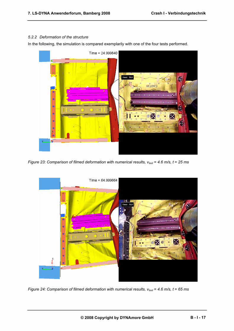
5.2.2 Deformation of the structure
In the following, the simulation is compared exemplarily with one of the four tests performed.
Figure 23: Comparison of filmed deformation with numerical results, vtest = 4.6 m/s, t = 25 ms
Figure 24: Comparison of filmed deformation with numerical results, vtest = 4.6 m/s, t = 65 ms
Crash I - Verbindungstechnik
B - I - 17
7. LS-DYNA Anwenderforum, Bamberg 2008
© 2008 Copyright by DYNAmore GmbH
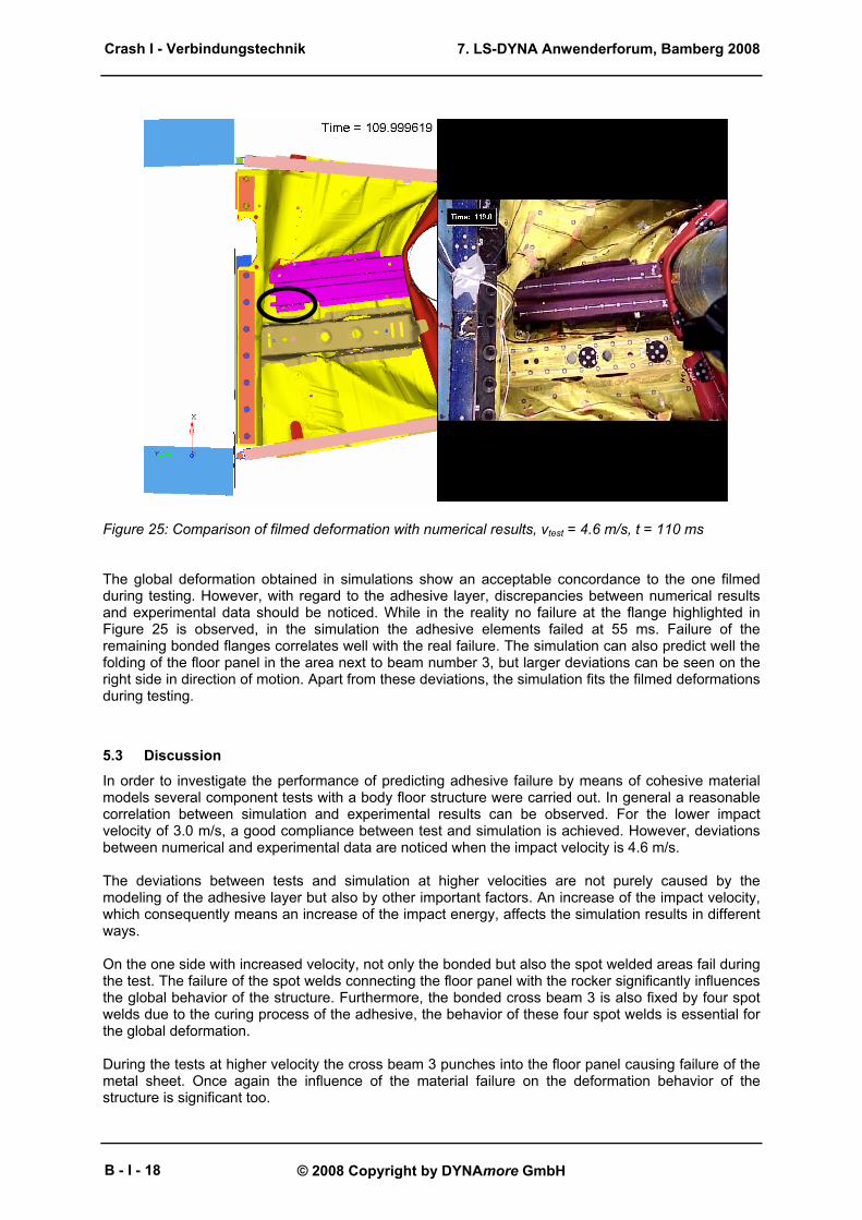
Figure 25: Comparison of filmed deformation with numerical results, vtest = 4.6 m/s, t = 110 ms The global deformation obtained in simulations show an acceptable concordance to the one filmed during testing. However, with regard to the adhesive layer, discrepancies between numerical results and experimental data should be noticed. While in the reality no failure at the flange highlighted in Figure 25 is observed, in the simulation the adhesive elements failed at 55 ms. Failure of the remaining bonded flanges correlates well with the real failure. The simulation can also predict well the folding of the floor panel in the area next to beam number 3, but larger deviations can be seen on the right side in direction of motion. Apart from these deviations, the simulation fits the filmed deformations during testing.
5.3 Discussion
In order to investigate the performance of predicting adhesive failure by means of cohesive material models several component tests with a body floor structure were carried out. In general a reasonable correlation between simulation and experimental results can be observed. For the lower impact velocity of 3.0 m/s, a good compliance between test and simulation is achieved. However, deviations between numerical and experimental data are noticed when the impact velocity is 4.6 m/s. The deviations between tests and simulation at higher velocities are not purely caused by the modeling of the adhesive layer but also by other important factors. An increase of the impact velocity, which consequently means an increase of the impact energy, affects the simulation results in different ways. On the one side with increased velocity, not only the bonded but also the spot welded areas fail during the test. The failure of the spot welds connecting the floor panel with the rocker significantly influences the global behavior of the structure. Furthermore, the bonded cross beam 3 is also fixed by four spot welds due to the curing process of the adhesive, the behavior of these four spot welds is essential for the global deformation. During the tests at higher velocity the cross beam 3 punches into the floor panel causing failure of the metal sheet. Once again the influence of the material failure on the deformation behavior of the structure is significant too.
Crash I - Verbindungstechnik
B - I - 18
7. LS-DYNA Anwenderforum, Bamberg 2008
© 2008 Copyright by DYNAmore GmbH
Finally the friction parameters in the global contact definition significantly dictate the global deformation behavior. One global contact is used for the analyses; values for the coefficients of friction are taken from experience.
6 Summary The increasing usage of adhesive bonding as a joining technique in vehicle structures requests simulation tools, which allow analysis of its crash behavior. Cohesive elements and cohesive material laws, which are available in the current LS-DYNA versions, may be chosen to model the adhesive layer. These models are commonly validated by comparing simulations of simple shaped test specimens to test results. However, the simulation of larger, geometrically more complex structures remains a challenge. The influences of the chosen technique of adhesive modeling, such as mesh size and connection possibilities to the bonded parts, are presented and discussed in the present paper. In any case, it should be carefully checked, if mass scaling can be used to reduce simulation time. A body floor structure with a cross beam bonded to a floor panel is tested at two velocities. Measured accelerations and videos containing the deformation of the tested component are compared to simulations. The cohesive zone model *MAT_138 together with interface elements is used to model the adhesive layer. A good agreement between simulation results and experimentally obtained data is observed in the presented work. The deviations between numerical and experimental results can be attributed not only to the behavior of the adhesive layer but also to other factors, such as friction, failure of spot welds or failure of the sheet metal. Therefore, new component tests with a cross beam purely connected by spot welds will follow to verify this hypothesis. To sum up, cohesive zone models seem to work well in crash analysis even for large structures. Care has to be taken concerning mesh quality and mass scaling, but generally acceptable results can be expected if coarse meshes are not used.
7 Literature [1] LS-DYNA Keyword User’s Manual, Volume I, Version 971, LSTC, May 2007 [2] Hesebeck, O., Nossek, M., Werner, H., Brede, M., Klapp, O., Klein, H., Sauer, M, Modeling of
Flexible Adhesive Joints in Automotive Crash Simulations: Calibration and Application of Cohesive Elements, Abaqus Users Conference, Paris, 2007
[3] Methodenentwicklung zur Berechnung von höherfesten Stahlklebverbindungen des Fahrzeugbaus unter Crashbelastung. Projektbericht P676, Forschungsvereinigung Stahlanwendung, 2008
Crash I - Verbindungstechnik
B - I - 19

7. LS-DYNA Anwenderforum, Bamberg 2008
© 2008 Copyright by DYNAmore GmbH
Crash I - Verbindungstechnik
B - I - 20

![Mario Marzi - IL SAXOFONO - (C) Zecchini Editore [Estratto]](https://static.fdocument.pub/doc/165x107/54a30ebbac7959791b8b460b/mario-marzi-il-saxofono-c-zecchini-editore-estratto.jpg)